a hierarchical feature representation for phonetic
TRANSCRIPT

A Hierarchical
Feature Representation
for Phonetic Classification
by
Raymond Y.T. Chun
Submitted to
the Department of Electrical Engineering and Computer Science
in Partial Fulfillment of the Requirements for the Degree of
Master of Engineering
at the
Massachusetts Institute of Technology
March, 1996
@Massachusetts Institute of Technology, 1996.
All rights reserved.
Signature of Author
Department of Electrical Engineering and Computer Science
March 4, 1996
Certified by .. ........... .......
James R. Glass
Principal Research Scientist
>'. Computer Science
Accepted by ......
;;ASSACHUSEhTS -
OF TECHNOLOGY
JUNI 1 1996
c R. Morgenthaler
Chair, Departmhent Committee on Graduate Students
Eng.LIBRARIES

A Hierarchical
Feature Representationfor Phonetic Classification
by
Raymond Y.T. Chun
Submitted to the Department of Electrical Engineering and Computer Science
in February, 1996 in partial fulfillment of the requirements for the Degree of
Master of Engineering
Abstract
The objective of this research is to investigate the use of a hierarchical frameworkfor phonetic classification of speech. The framework is motivated by the observationthat a wide variety of measurements may be needed to make phonetic distinctionsamong different types of speech sounds. The measurements that best discriminateamong one class of sounds will most likely be suboptimal for other classes. By allowinga succession of measurements, a hierarchy ensures that only the meaningful featuresare used for each phonetic distinction. Furthermore, by partitioning phones intoclasses, a hierarchy provides some broad context for making finer phonetic distinctionsamong confusable sounds.
In the hierarchies explored in this thesis, a speech segment is initially classifiedinto a broad phonetic class using a feature set targeted towards making the broaddistinction. Probability scores are assigned to each phonetic class, reflecting thelikelihood that the speech segment belongs to the broad class given the featuresextracted at that stage. Subsequent stages classify the segment into successively finersubclasses, again producing intermediate class probabilities based on feature setsoptimized for each particular stage. Overall phone scores are then computed withinan MAP probabilistic framework which combines all relevant class scores, allowingmeaningful comparisons to be made across all phones.
A set of classification experiments are performed on the TIMIT acoustic-phoneticcorpus. A set of baseline experiments are established which represent state of the artclassification results for the vowels and all phones. Hierarchical classification resultsindicate that overall performance can be improved by raising scores at individualnodes in the hierarchy. The improvements reported in this thesis reflect gains ofless than half percent, but larger gains are expected with the use of more rigorouslyoptimized feature sets.Thesis Supervisor: James R. GlassTitle: Principal Research Scientist

Acknowledgements
I wish to express my sincere thanks to my thesis supervisor, Dr. James Glass, forthe thoughtful consideration he has given to all aspects of this thesis. His insight andvision have guided this work from start to finish. I truely appreciate the dedicationwhich he has shown to me.
I am grateful to Dr. Victor Zue for providing me with the opportunity to workwith so many extraordinary individuals. His magnanimity has made the SLS groupa wonderful place to conduct research.
I would like to thank the following people for their contributions to this thesis:Special thanks to Mike McCandless for reshaping the speech recognizer into a formeasily accesible to all, and to my officemate Jane Chang, for answering all my ques-tions.Helen Meng and Stephanie Seneff (and Jim Glass, of course) for proofreading mythesis.All members of the Spoken Language Systems group, for their friendly nature.Frank, Joe, and Susan, for making my experience at MIT an enjoyable and memorableone.My sister, mother, and father, for their love and support.

Contents
1 Introduction
1.1 Speech Knowledge for Phonetic Classification
1.2 Probabilistic Pattern Classification . . . . . . . .
1.3 Hierarchical Framework ..............
1.3.1 Hierarchical Structures............
1.3.2 Probabilistic Framework for the Hierarchy
1.4 Brief Summary of Previous Work
1.4.1 Uses of Hierarchies .............
1.4.2 Broad Class Partitions . . . . . . . . . . .
1.5 Thesis Overview....................
2 Baseline Experiments
2.1 Background and System Overview . . . . . . . . .
2.1.1 Corpus.....................
2.1.2 System Components ............
2.2 Acoustic Modelling .................
2.3 Calibrating the Posterior Probabilities . . . . . .
2.4 Results.. . . . . . . . . . . . . . . . . . . . .. . .
2.5 Chapter Summary .................
3 Hierarchical Phonetic Structures
9
.. .... .. .. 10
.. .... ... . 12
.. .... ... . 14
.. .... ... . 14
... ... .... 17
...... ... . 19
.......... 19
. . . . . . . . . . 20
.... ... ... 22
24
. . . . . . . . . . 24
.... .... .. 24
. ... .... .. 25
. ... .... .. 29
. . . . . . . . . . 31
. ... .... .. 34
. ... .... .. 35
37

3.1 A Hypothetical Hierarchy ............... ......... 37
3.2 Class-based Hierarchies ................ ........ .. 38
3.2.1 Heterogeneous Feature Sets .................... 41
3.3 Clustering based on confusability ................... . 46
3.3.1 Properties of Strong Fricatives and Affricates ......... .47
3.3.2 Results and Discussion ..................... . 49
3.3.3 Multiple Class Membership ................ . . . . 50
3.4 Chapter Summary ........................... .. 53
4 Pruning 54
4.1 Results .......... ............. ... ..... .... .. 55
4.2 Chapter Summary ............................ 58
5 Conclusions and Future Directions 61
5.1 Sum m ary ...................... ........... .. 61
5.2 Future Directions ..... ............. ... ... ..... .. 62
A Confusion Statistics 65
A.1 SONORANT vs. OBSTRUENT vs. SILENT partition ......... 65

List of Figures
1-1 Spectrogram of the utterance, "Two plus seven is less than ten." . . .
1-2 Hypothetical Gaussian distributions for VOT for [b] and [p] . . . . .
1-3 Sample hierarchical classification of [9] phone . . . . . . . . . . . . .
1-4 Sample hierarchical classification of [9] phone . . . . . . . . . . . . .
2-1 Triangular Mel-scale Filters .......................
2-2 Baseline performance as the minimum number of data points is varied.
2-3 Histogram of probability estimates . . . . . . . . . . . . . . . . . . .
2-4
2-5
2-6
2-7
3-1
3-2
3-3
3-4
3-5
3-6
3-7
Histogram of probability estimate ratio . . . . . . . . . . .
Effect of varying P on probability estimates . . . . . . . .
Effect of varying / on baseline performance . . . . . . . .
Baseline performance as the number of cepstral coefficients varied. .
Manner based hierarchy (Manner tree). ................... 39
Hierarchy by voicing and speech (SOS tree) ................ 39
Combined hierarchy (3 LVL tree). .................... . 39
Vowel classification accuracy for feature subsets. .............. 45
Tree targeting the [s] vs [z] distinction .................. 48
Tree formed by clustering based on confusability ............. 49
Variable realizations of the [6] phone. .................... 51
4-1 Classification accuracy with pruning ...... S 56

4-2 Computation required, as percentage of baseline. ............. 56
4-3 Classification accuracy after pruning all but the n-best class models.. 57
4-4 Computation required, as percentage of baseline ............. 59
4-5 Inclusion of correct model within top n scores .............. 59

List of Tables
1.1 Distinctive feature representation. .................... . 21
2.1 Comparison of train and test sets . . . . . . . . . . . . . . . . . . . .
2.2 IPA symbols for phones in the TIMIT corpus with example occurrences
2.3 39 phone classes used by Lee [10] . . . . . . . . . . . . . . . . . . . .
2.4 Phonetic classification accuracies . . . . . . . . . . . . . . . . . . . .
Broad classes and constituent phones . . . . . . . . .
Phone and class accuracies . . . . . . . . . . . . . .
Phonetic accuracy across various phonetic subclasses.
16 vowels used in previous experiments.. . . . . . . .
Comparison of train and test sets for vowel studies..
Conditions and results for previous vowel classification
Vowel classification accuracies . . . . . . . . . . . . .
Phones in the vowel subset . . . . . . . . . . . . . .
Performance for the hierarchy using FO information.
Phonetic confusions among the strong fricatives . . .
Confusions among the SON, OBS, and SIL classes.
Phones with significant confusions . . . . . . . . . .
Reassigned labels.. . . . . . . . . . . . . . . . . . . .
experiments.
A.1 Phone confusions ......................
3.1
3.2
3.3
3.4
3.5
3.6
3.7
3.8
3.9
3.10
3.11
3.12
3.13

Chapter 1
Introduction
Speech is produced by a series of closely coordinated articulatory gestures that re-
sult in a sequence of sounds called phones. Due to similarities in the production of
these phones (e.g., in the manner or place of articulation), phonetic classes naturally
emerge whose constituent phones exhibit common acoustic-phonetic properties [4].
Sonorant phones, for instance, are produced with a periodic excitation at the glottis
and collectively exhibit a low frequency periodicity in the speech waveform. Phones
in other classes, however, are characterized by different features, and require the use
of different acoustic cues to distinguish. Stop consonants in particular have few traits
in common with sonorant phones, and require a more temporal approach to signal
analyis [28]. In this thesis, we explore a hierarchical feature representation in which
different cues can be considered for unrelated classes of sounds, allowing the use of
targetted features for making fine phonetic distinctions among confusable phones.
The effectiveness of the hierarchical framework is evaluated on the phonetic clas-
sification task. We choose this task because it isolates the problems associated with
the feature representation and acoustic modelling from those of the segmentation,
and does not rely on higher order language constraints. Though our task will end

with phonetic classification, we believe that improvements in this task will ultimately
be reflected by improvements in phonetic recognition, which in turn should lead to
higher accuracies at the word and sentence level [10].
1.1 Speech Knowledge for Phonetic Classification
In this thesis, much of the intuition for structuring the hierarchy is based on a knowl-
edge of the acoustic features which define and differentiate classes of phones. We
need speech-specific knowledge to guide us in creating the phonetic classes, as well as
in optimizing the feature sets for use within each class. Even with automated proce-
dures, it is important that we use speech knowledge in order to establish reasonable
criteria for selecting the classes and features.
There are many different sources of speech knowledge available to us. We can
consult models of speech production and perception to determine what is acoustically
important and what is irrelevant, with the assumption that the auditory system
is best matched to the decoding of the speech waveform. We can also study the
waveform indirectly, in the form of a spectrogram, since the waveform must contain
all information necessary for making phonetic distinctions, and the spectrogram, we
presume, retains much of that information.
One observation we can make from reading spectrograms is that there are different
types of acoustic cues associated with different types of speech sounds. In particular,
not all acoustic features are equally important for a given phonetic distinction. We
demonstrate this with the spectrogram in Figure 1-1.
We can see that certain portions of the spectrogram are characterized by formants
(e.g., from 0.25 to 0.4 s, or from 1.0 to 1.1 s), indicating, in general, a vocalic seg-
ment. These formants are important for differentiating among phones in the vowel
class. However, for the fricatives centered around 0.45 s and 1.2 s, extracting formant
information would be uninformative, since there are no low frequency resonances to

kHz 4 kHz
0
Figure 1-1: Spectrogram of the utterance, "Two plus seven is less than ten."The spectrogram displays the spectral components of the utterance against time.
observe. Instead, we might look at the low frequency energy, the high frequency
energy cutoff, duration, formant transitions in adjacent vowels, or the intensity of
frication.
As Zue, Cole, and others [29, 2] have demonstrated, we can use spectrograms to
discover acoustic features for specific speech sounds. In particular, we can discover
acoustic features for making fine distinctions between confusable phones such as [b]
and [p], or [m] and [n]. This is necessary for good recognition, since many words
share the same broad class representation but differ in one phone. For instance,
when recognizing the word 'bear,' we may be unable to eliminate the confusable
candidates such as 'pear,' or 'beer,' without higher order language constraints. A
detailed inventory of acoustic cues would be crucial in such a circumstance.
In order to make the detailed decisions described above, we need to first classify
speech segments into meaningful phonetic classes. We can use our knowledge of the

speech production process to select these classes. Studies indicate that phones with
the same manner of articulation, i.e., phones that are produced in similar ways, are
highly confusable [18]. For example, [m] and [n] both have similar spectral profiles
during the period of oral closure [5]. An examination of the formant transitions
surrounding the two phones is needed to distinguish them. Other class groupings are
worth investigating, based on place of articulation or confusability.
1.2 Probabilistic Pattern Classification
We would like to develop a mathematical framework in which observations in differ-
ent feature spaces, corresponding to sets of measurements uniquely defined for each
phonetic class, can be combined together so that meaningful comparisons can be
made across all phones. For this thesis, we use a probabilistic formulation based on
a maximum a posteriori (MAP) decision strategy. In this formulation, the goal of
phonetic classification is to determine the most probable phone given the acoustic
feature vector for the speech segment. If we represent the phone set as {ai}, and the
n-dimensional acoustic feature vector as {f = fo, fi, f2,... , fn- }, we can express the
problem mathematically as arg maxPr(ai I f).
In its simplest form, the MAP decision strategy can be used to decide between two
hypotheses given a single measurement. For example, suppose we wish to classify a
speech segment as either a [b] or a [p] using voice onset time(VOT). Figure 1-2 shows
the probability distributions of the two phones as might be expected using the VOT
attribute.
For a given VOT measurement, the acoustic score Pr(VOT I Hi) under each
hypothesis Hi (i = 0, 1) is determined, and then each score is scaled by a factor
proportional to its prior probability to obtain the posterior probabilities Pr(Hi I

Pr(VOTl[p])
VOT
Figure 1-2: Hypothetical Gaussian distributions for VOT for [b] and [p].
VOT). The exact relationship is described by Bayes' rule:
Pr(VOT I Hi)Pr(Hi)Pr(H; I VOT ) = (1.1)Pr(VOT)
The higher of the two posteriors is selected as the score representing the correct
hypothesis. In practice, since the denominator term in Equation 1.1 is identical for
every Hi, it can be disregarded, so that the decision rule reduces to choosing Hi that
satisfies:
arg max Pr(VOT I Hi)Pr(Hi) (1.2)
Note that if the a priori probabilities are the same, (that is, if Pr(Hi) = Pr(H2)),
then the decision rule reduces to a maximum likelihood decision, in which the greater
of the two likelihood terms is chosen as the correct hypothesis.
In this thesis, we use mixtures of Gaussians to approximate the underlying distri-
bution of the phones [22], so that the likelihood for any given feature f is computed
as,
Pr(f H) = H Pr(f I mj, Hi)Pr(mj I Hi) (1.3)
where mj represents the jth Gaussian mixture. The likelihood associated with each
mixture is summed to determine the total likelihood for that feature, which is scaled
Pr(

as explained above to produce the phone's posterior.
1.3 Hierarchical Framework
In the baseline configuration for classification, the entire set of features is used for
classifying all speech sounds. One of the problems with a uniform feature vector is
that not all features are relevant to identifying any one particular phone, as is the
case when examining VOT when the segment is a vowel. At such times, the irrelevant
features introduce the equivalent of noise into the feature space, since the likelihoods
associated with these features are not indicative of the underlying phone. In some
cases, the contributions from all extraneous features may even corrupt the overall
phone posterior, so that the wrong phone is hypothesized. An alternative framework
is provided by a hierarchy. In a hierarchy, we can select a subset of meaningful features
for each phonetic decision, thus minimizing the dimensionality of the feature space
and possibly increasing the robustness of the acoustic models at each node.
It is important to note that the performance of the hierarchy is as much affected
by the choice of phonetic classes as by the choice of features for each class, since it is
the class structure that determines the types of phonetic distinctions which must be
made. Thus, in addition to optimizing features for each node, we must consider the
effectiveness of different phone groupings.
1.3.1 Hierarchical Structures
Meaningful classes will ensure both a compact feature representation and efficient
acoustic modelling, both of which are important factors affecting the performance
of the hierarchy. We can conceive of several different ways to arrive at a reasonable
tree structure. The simplest method is to select classes manually, based on acoustic-
phonetic knowledge or confusion statistics. Intuitively, we would like the more robust
decisions to occur first, since later decisions will be influenced by these parent nodes.

Accordingly, we reserve the most confusable decisions for the leaf nodes, where we
discriminate among a much smaller set of acoustically similar phones. Figures 1-3
and 1-4 show sample tree structures which might arise with these objectives in mind.
The darkened line in Figure 1-3 indicates the correct path for classifying a [9]
phone. Note that since phones are mapped to individual classes, there is only one
path that correctly classifies each speech segment. In this case, the highest scoring
path must include either the OBSTRUENT and STRONG FRICATIVE classes.
Alternatively, we can allow phones to belong to multiple phonetic classes. Though
we can theoretically give all phones membership to all classes, this would be com-
putationally taxing and probably unwarranted, since a phone like [S] will rarely get
confused with a phonetic class consisting of vowel tokens. A more reasonable approach
is to select just those phones which are confusable with more than one phonetic class,
and extend membership for those phones. Probability scores are computed for all
possible paths, and then summed to arrive at an overall score.
As illustrated in Figure 1-4, we can, under this scheme, allow for the possibility
that the [9] might be realized with little energy, and provide a means for scoring
the [9] as both a STRONG or WEAK fricative. This method acknowledges that a
phone may have more than one group of confusable partners. For instance, the [s] is
confusable with [z] at times and [0] at other times. Using separate paths, different
features can be used for making these two distinctions. (Similarly, multiple branches
can represent the same set of phones, to account for the fact that different cues can
independently indicate the presence of a phone. The difference between an [s] and a
[z] might be voicing on the one hand, and duration on the other. A simple threshold
might suffice in this case).
Automatic methods for clustering phones into classes would presumably lead to
trees with the same overall structure as those created manually. That is, given our
knowledge of acoustic-phonetics, and the empirical evidence to guide the selection
of confusable phone sets, it is unlikely that automatic procedures for defining pho-

OBSTRUENT
STRONGFRICATIVE
[S] * * * [S] [Z]
OTHER
OTHER
Figure 1-3: Sample hierarchical classification of [9] phone.
STRONGFRICATIVE-LIKE
WEAKFRICATIVE-LIKE
[S] [ZS* * * [S] [Z]s [F] [V]"
Figure 1-4: Sample hierarchical classification of [9] phone.
OTHER
[SL[Z],

netic classes will result in a significantly different tree structure. The more valuable
application of automatic procedures might be in developing features for the classes.
A more involved method for developing a hierarchy is to start with a list of features,
derived either manually or automatically, and allow our choice of features to dictate
the partitioning of the phones into natural phonetic classes. Thus, for instance, we
could use a voicing feature and observe the phones divide into SONORANT and
OBSTRUENT classes. This appears to be a natural way to partition phones, since
phones may be characterized by different bundles of features at different times, and
thus belong to different phonetic classes on different occasions. Then, we would be less
susceptible to modelling errors caused by inconsistencies in the phonetic realizations,
since the acoustic models would be trained only on well-formed tokens.
1.3.2 Probabilistic Framework for the Hierarchy
It was stated that the goal of phonetic classification is to determine i that satisfies
arg max Pr(aj I f). In the hierarchical approach, we are further interested in the
probability that the phone belongs to a particular broad class Cj given the acoustic
data, expressed as Pr(ai E Cj I f). For compactness, we will express this simply as
Pr(Cj I f). If the classes are collectively exhaustive, we can expand Pr(a I f) into
the equivalent expression:
Pr(a I f) = EPr(ai I Cj,f)Pr(Cj I f) (1.4)
Equation 1.4 describes the hierarchical scheme depicted in Figure 1-4, in which phones
are members of multiple classes, and the overall phone posteriors are computed as
the sum of all path scores.
If, on the other hand, we assume that each phone belongs to a single class, the

summation in equation(1.4) can be discarded, leaving:
Pr(ai I f) = Pr(ai I Cj,f)Pr(Cj I ) (1.5)
where Cj is the assigned class for phone ai. This is the simplified case depicted in
Figure 1-3. The framework can be readily extended to additional stages. Introducing
a subclass Ck of class Cj to the tree, the expression in (1.5) becomes:
Pr(ai I f) = Pr(ai I Ck,f)Pr(Ck I Cj,f)Pr(Cj I f) (1.6)
We now make the assumption that each class probability can be more accurately
derived using a subset of features contained in f. These sub-vectors, which we will
denote using {fa, fb,...}, together constitute f such that fa U fb U ... = f. Then, we
are left with:Pr(Cif., fa, fbc - )
Pr(Ci I f)= Pr(C I Jfab,...)= r #,, f,...) (1.7)Pr(fa, fb, fc,...)
Pr(Cifa)Pr(fb, f,,...) r( ) (1.8)- -# = Pr(Ci I fa) (1.8)
Pr(fa)Pr(fb, fc, ,..)
Note that we must assume independence between feature subsets in order to justify
the term expansion between equations 1.7 and 1.8.
Finally, since each node of the tree uses a different subset of the feature vector,
equation (1.5) becomes:
Pr(a, I f) a Pr(ao I Cj,fa)Pr(Cj I fb) (1.9)
Bayes' rule is applied to each of the terms on the right hand side to rewrite the

equation in a more convenient form. Each term is expanded as follows:
S Pr(fa Cj)Pr(Cj)Pr(CjI fa) - (1.10)Pr(fa)
where Pr(fa) = ZPr(fa I Cj)Pr(Cj) (1.11)
The calculation is identical at the leaf nodes, since phones may be thought of as single
member classes.
1.4 Brief Summary of Previous Work
1.4.1 Uses of Hierarchies
Hierarchies incorporating speech knowledge have been developed for various speech
related tasks. In the early 1980's, FEATURE, an alphabet recognition system de-
veloped by Cole et al [2], demonstrated the effectiveness of using speech knowledge
within a hierarchical framework. The system relied on manually chosen sets of fea-
tures to classify speech segments into successively smaller classes of letters, computing
posterior probabilities at each node of the tree. The a posteriori probability for each
letter was obtained by chaining together all of its prior class probabilities, and the
letter with the maximum posterior probability was the one hypothesized.
In this thesis, we adopt a similar approach, but apply our hierarchy to the identi-
fication of phones rather than isolated letters. Using phones as the basic recognition
units allows the hierarchy to be applied to other tasks such as word recognition. How-
ever, because we have generalized the problem, there are fewer constraints and more
variabilities to account for in classifying each segment. For instance, in phonetic clas-
sification, there is a larger inventory of sounds. Furthermore, we must now account
for co-articulation across segments, since one phone can affect the characteristics of
its neighbors.

In 1985, Leung [15] developed a decision tree based on broad classes for use in
automatically aligning a speech waveform with its phonetic transcription. He used
a binary classifier to classify speech segments into one of five broad phonetic classes
under the premise that an initial broad segmentation, insofar as it is both reliable
and constraining, could serve as an anchor point around which the more confusable
segments could be aligned. His use of a binary decision tree was motivated by the
increased flexibility with which he could partition the feature space, an advantage
inherent in any hierarchical classifier. One significant difference, however, between
Leung's system and the hierarchy we investigate is that we assign likelihoods to each
broad class, whereas Leung makes a hard decision at each node, resulting in a single
class being proposed. This suffices for his task, which only requires that a broad
class be hypothesized, but since we require further classification into phones, some
measure of relative likelihoods must be incorporated into our hierarchy. This allows
us to analyze all acoustic data before committing to a particular phonetic class.
In 1992, Grayden and Scordilis [7] developed a hierarchy for classifying obstru-
ent phones in continuous speech. They used Time-Delay Neural Networks for most
class decisions (a simple threshold on low frequency energy was first used to elimi-
nate sonorants). Their system demonstrates the feasibility of applying hierarchies to
classification at the phone level. In this thesis, we extend classification to include all
phones and use mixtures of full covariance Gaussian classifiers.
1.4.2 Broad Class Partitions
Since a broad class representation is a natural intermediate stage in our tree struc-
ture, the constraints provided by such a representation are of interest to us and lend
appeal to the development of a class-based hierarchy. Various studies in the past
have been related to partitioning phones into classes. In 1982, Shipman and Zue [26]
demonstrated that a broad class representation based on manner of articulation could
pare a 20,000 word vocabulary down to a manageable set of candidates. Studies had

Feature i I u E O 0high + + + --low - - - - - +back - + + +labial - - + - + -tense + + + - + -
Table 1.1: Distinctive feature representation.
shown that perceptual confusions were common among phones within a manner of
articulation class [18].
Alternative class partitions based on distinctive features have also emerged. Dis-
tinctive features are a way of representing phones using a set of binary indicators
that correspond to the minimal difference between phones [16]. Table 1.1 lists some
vowels and their distinctive features.
Stevens [27] has placed these features in a hierarchy since certain features are more
easily identified once other features are known.
An interesting property of distinctive features is that since they can discriminate
between two phones that are minimally distant, they are equally suited for making
broad and fine phonetic distinctions. For instance, we can partition the vowels in
Table 1.1 into two classes of sounds using the feature tense, and then use combinations
of the other features to discriminate further among the candidates. However, we can
also first eliminate all phones except for [i] and [i] using all features except for the
feature tense, and then use tense to make the final distinction between the two. This
property makes distinctive features both simple and powerful.
In 1989, Meng [16] performed vowel classification experiments using an MLP clas-
sifier in which the spectral representation was mapped to an intermediate distinctive
feature representation before accessing the lexicon. If the features were assigned bi-
nary values then performance dropped, as this required all distinctive features to be

correctly determined. However, if the distinctive feature scores (i.e., the probability
estimates for the distinctive features, obtained using an MLP classifier) were fed into
a second MLP, classification accuracy was comparable to that of the bare spectral
representation.
The mapping to distinctive features can be viewed as a hierarchy in which each
node generates a score for a different feature. Assigning the features binary values
equates to making a hard decision at each node, which agrees intuitively with the
decrease in performance. Her work indicates that an intermediate representation can
potentially offer better performance, but it requires more careful consideration for
the acoustic attributes before improvements can be demonstrated.
1.5 Thesis Overview
This thesis attempts demonstrate the feasibility of a hierarchical feature representa-
tion. The framework for scoring is based on a MAP decision rule that allows fair
comparison across disjoint observation spaces. Initial experiments in chapter 2 es-
tablish a baseline system within that framework. The behavior of the probability
estimates is observed to ensure that the MAP framework is functional. A correction
factor is introduced to ensure healthy probability estimates using the baseline feature
vector.
In chapter 3, we evaluate hierarchical structures, and investigate methods for rais-
ing classification scores. We begin with manually determined trees, and demonstrate
the feasibility of heterogeneous feature sets for different classes of sounds. Specifically,
we increase vowel classification scores by augmenting the baseline feature vector with
a measure of pitch, and then demonstrate that these improvements translate into
overall classification gains.
We also explore a bottom-up clustering approach, in which confusable sounds
are merged into classes. In order to constrain the phone space, this experiment is

performed only on the strong fricatives and affricates. Again, we use heterogeneous
feature sets (this time subsets of the baseline feature vector) and demonstrate that
improvements can be made overall.
In Chapter 4, we study the use of pruning thresholds to save computation. Since
more robust decisions are made at the broad class level, we can reliably eliminate
subsections of the hierarchy for which the broad class model scores poorly. This has
implications for lexical access and fastmatch.
Chapter 5 summarizes the work presented in this thesis and suggests directions
for future work.

Chapter 2
Baseline Experiments
In this chapter, we resolve modelling issues associated with the hierarchy, and incor-
porate the constraints in evaluating the baseline. In addition, we assess the effec-
tiveness of the MAP framework in computing posterior probabilities by performing
experiments with the baseline system.
2.1 Background and System Overview
2.1.1 Corpus
Experiments are conducted on the publicly available TIMIT acoustic-phonetic corpus,
which has been widely used for phonetic classification and recognition studies [11].
The TIMIT database provides speaker-independent, continuous-speech from both
male and femaler speakers, 1 together with time-aligned phonetic transcriptions of
all utterances. We use 8 sentences from each speaker, of which 3, the 'si' sentences,
are phonetically diverse and unique to a given speaker. The remaining 5 'sx' sentences
'The database represents 8 dialect regions of American English. 70% of the speakers are male,and 30% female.

are phonetically compact and are repeated by other speakers. Table 2.1 lists the sets
used or cited in this thesis. Unless otherwise noted, test accuracies are reported on
the NIST TEST set using models trained from NIST TRAIN. All optimization are
performed on NIST DEV, which is configured such that there is no overlap among
utterances in DEV and TEST. The train set MIT TRAIN 2 has been developed for
simplicity and consists of all NIST utterances excluding those in MIT TEST. It is
nearly identical to MIT TRAIN, but contains 13 additional speakers.
SET #SPEAKERS #UTTERANCES #TOKENSNIST TRAIN 462 3,696 sx, si 142,910NIST TEST 118 944 sx, si 35,697NIST DEV 50 400 sx, si 15,057MIT TRAIN 567 4,536 sx, si 175,101MIT TRAIN 2 580 4,640 sx, si 133,988
Table 2.1: Comparison of train and test sets.
The phonetic transcriptions in the TIMIT database specify 61 different phone
labels, listed in Table 2.2. For testing, we collapse these labels to a set of 39 classes
developed by Lee [12], as is commonly done in reporting accuracies. The collapsed
set is shown in Table 2.3. In addition, glottal stops are ignored, both in accordance
with Lee and because the glottal stops in particular are difficult to group with other
phones.
2.1.2 System Components
For this thesis, since we deal only with the task of phonetic classification, we are
only interested in the front end components of recognition. In these early stages, the
acoustic signal is transformed into a signal representation which holds the signal's
phonetic information in a more compact form. A feature vector is then computed
from this representation for each segment of speech. Finally, the Bayesian classifier

IPA TIMIT Example IPA TIMIT Examplea aa bob I ix debitae ae bat i iy beetA ah but j jh joke3 ao bought k k keyOa aw bout ka kcl k closurea ax about 1 1 layah ax-h suspect m m moma axr butter n n noonoY ay bite 13 ng singb b bee nx winnerbO bcl b closure o ow boate ch choke Y oy boyd day p p peado dcl d closure o pau pause6 dh then P1 pcl p closurer dx muddy ? q batE eh bet r r ray1 el bottle s s seam em bottom 9 sh shen en button t t tea0 eng Washington to tcl t closurel epi epenthetic silence 0 th thin
3" er bird o uh booke ey bait u uw bootf f fin ii ux tootg g gay v v vangP gcl g closure w w wayh hh hay y y yachtfi hv ahead z z zoneI ih bit 2 zh azure
- h# utterance initial and final silence
Table 2.2: IPA symbols for phones in the TIMIT corpus with example occurrences

a, a
A, 9, 9h
A7, 3a'
bbo, 1p0, dO, to, 9P, kO
d6£
14151617181920212223242526
i, 1m, mn, n,0, 0efgh, fiI, Ii
Jko
Table 2.3: 39 phone classes used by Lee [10]
compares acoustic models with this feature vector and selects the most likely phone.
Below, we summarize the pertinent aspects of this process.
Signal Representation
The baseline system uses a Mel-based signal representation that is characterized by
a warping of the frequency axis to approximate the frequency response of the ear
[17]. First, the speech waveform is sampled at 16 kHz and windowed with a 20.5 ms
Hamming window advanced at a 5 ms frame rate. The 20.5 ms window size was deter-
mined to be optimal through preliminary experiments using a baseline configuration
roughly equivalent to the one used in this thesis. A power spectrum is then computed
for each segment by squaring the 256 Fourier coefficients obtained from a simple DFT
on the windowed speech samples. A set of 40 triangular filters is used to compress
the 256 power spectral coefficients into 40 Mel-frequency spectral coefficients (MFSC)
[16]. As Figure 2-1 shows, these filters are spaced further apart at high frequencies
since the ear cannot discriminate as well among high frequency sounds. Finally, a
12345678910111213
27282930313233343536373839
DYPr
s
1, 2t0oU,u, UivVwWYz

0 2000 4000 6000Frequency (Hz)
Figure 2-1: Triangular Mel-scale Filters
cosine transform converts the MFSC to 40 Mel-frequency cepstral coefficients, the
first 12 of which are used in the feature vector.
Feature Vector
The baseline feature vector consists of 12 MFCC's averaged across thirds of the seg-
ment, as well as MFCC derivatives taken at the start and end of the segment and the
log of the segment duration. 12 MFCC's was found to be optimal for the classification
task on the NIST DEV set (see Figure 2-7).
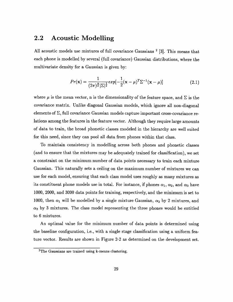
2.2 Acoustic Modelling
All acoustic models use mixtures of full covariance Gaussians 2 [3]. This means that
each phone is modelled by several (full covariance) Gaussian distributions, where the
multivariate density for a Gaussian is given by:
1 1Pr(x) = exp[- (x -1 )X 1 (x - p)] (2.1)
(27r) 2j 2 2
where y is the mean vector, n is the dimensionality of the feature space, and E is the
covariance matrix. Unlike diagonal Gaussian models, which ignore all non-diagonal
elements of E, full covariance Gaussian models capture important cross-covariance re-
lations among the features in the feature vector. Although they require large amounts
of data to train, the broad phonetic classes modeled in the hierarchy are well suited
for this need, since they can pool all data from phones within that class.
To maintain consistency in modelling across both phones and phonetic classes
(and to ensure that the mixtures may be adequately trained for classification), we set
a constraint on the minimum number of data points necessary to train each mixture
Gaussian. This naturally sets a ceiling on the maximum number of mixtures we can
use for each model, ensuring that each class model uses roughly as many mixtures as
its constituent phone models use in total. For instance, if phones al, a 2, and as have
1000, 2000, and 3000 data points for training, respectively, and the minimum is set to
1000, then al will be modelled by a single mixture Gaussian, a2 by 2 mixtures, and
a 3 by 3 mixtures. The class model representing the three phones would be entitled
to 6 mixtures.
An optimal value for the minimum number of data points is determined using
the baseline configuration, i.e., with a single stage classification using a uniform fea-
ture vector. Results are shown in Figure 2-2 as determined on the development set.
2The Gaussians are trained using k-means clustering.

There is a clear peak between 750 and 1000, with performance declining on either
'70
I1
CZ)
S77
o
• 76C,,r-.
7
'7IC0 1k 2k
Minimum Data Points
Figure 2-2: Baseline performance as the minimum number of data points is varied.
side. Above 3000 data points, only one full covariance Gaussian is being trained for
most phones, so classification accuracy remains constant. Below 200 points, accuracy
decreases dramatically.
The highest score is obtained with a minimum of 900 data points per Gaussian.
The corresponding number of mixtures used for each phone varies between 1 and 8. In
subsequent experiments with phonetic classes, we assume 900 minimum data points
to be sufficiently optimal, so that optimizations concerning the number of mixtures
for the phonetic class models will not be made.
rJ

2.3 Calibrating the Posterior Probabilities
Preliminary experiments with the baseline system have demonstrated that the phone
posterior probability scores obtained using the MAP framework are not accurate
indications of the actual probabilities of the phones given the acoustic data. In order
to correct for these mis-estimates, we observe their behavior using histograms of the
estimates across all tokens in the NIST development set. Specifically, we keep a count
of the probabilities estimated when the correct phone model is used to evaluate the
speech segment, as well as when all phone models (including the correct one) are
used. Figure 2-3 shows these counts.
Each plot represents a histogram H(x) for probabilities x between 0 and 1. The
solid line can be explained as follows. If we let cra represent the correct phone for
a given speech segment S, then Hsotid(x) = Cnt{Pr(a, IS) = x}, where the term
on the right hand side represents the number of times that the correct phone model
hypothesizes a probability estimate of x. The Hsolid(x) is appropriately high for
probabilities x near 1, but it is also high for probabilities near zero. This is a clear
indication that not all of the features used for evaluating the segments are meaningful.
It could be that there are too many extraneous features generating low likelihoods.
A more efficient feature vector might alleviate this problem.
Similarly, the histogram drawn with the dotted line represents the count across
all phones, not just the correct one. So, Hdotted(X) = Cnt{Pr(aC ( S) = x}Vi, where
{ a } represents the phone set . Since Hdotted(x) represent both correct and incorrect
phone probability estimates, it should closely follow Hsolid(x) for high probabilities,
but have most of its mass at the low probabilities. This is approximately indicated
in the figure.
If we plot the ratio of the correct histogram to the total, we measure the rela-
tionship between our estimated posterior and the experimentally observed posterior
(Figure 2-4). Ideally, the slope should be 1:1, representing a linear correspondence

e"0
102Ez
102
InI
0 0.1 0.2 0.3 0.4 0.5 0.6 0.7 0.8 0.9Probability Estimate
Figure 2-3: Histogram of probability estimatesProbability estimate counts using the correct phone model (solid line) and all phone
models (dotted line).
.oiiiEa0
Probability Estimate
Figure 2-4: Histogram of probability estimate ratioNumber of occurrences of a given probability estimate using the correct phonemodel, scaled by the number of occurrences of that probability estimate by all
models.
iLr:I·I
II
_I
rr I,,

between estimated and actual probabilities. We can see that instead, Pr(a I f) gen-
erally underestimates Pr(a I f ) .
One remedy for this problem is to alter the amount of influence given to the
phone's a priori probability, relative to the phone's acoustic score. Specifically, the
probability estimates have been computed using Bayes' rule:
Pr(f I aj)Pr(aj) (2.2)Pr(a I f) - A (2.2)SPr(f I aPr(a)
In the numerator, we have a probability estimate based on the extracted feature vector
(the left term) and an a priori probability estimate. By weighting the likelihood term,
as shown in equation (2.3), with an exponential scaling factor #, we can readjust the
probability estimates to more closely approximate the actual probabilities. Because
the denominator term under the expansion acts simply as a scaling factor, we can
ignore it in this discussion.
Pr(f Iaj) [Pr(f I aj)]O (2.3)
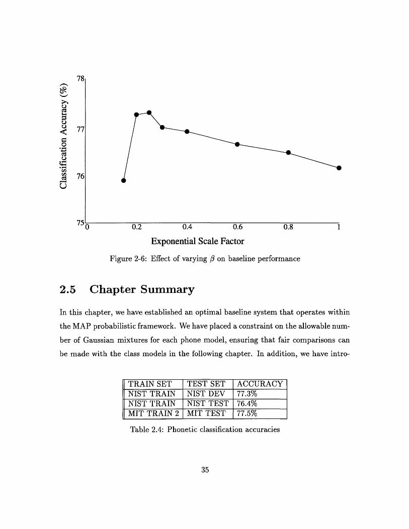
The effect of 3 on the accuracy of the probability estimates can be seen in the plots
of figure (2-5). For / near 0.3, we have a near linear relationship between Pr(a I f)
and Pr(a I f). For lower and higher values of /, Pr(a I f) is a warped representation
of Pr(a I f). The plot in figure (2-4) corresponds to a P of 1, i.e., an unweightedestimate. The actual classification accuracies (on the NIST development set) using the
exponential scaling of acoustic scores are shown in figure 2-6. As we would expect, the
higher classification scores correspond to the plots that have a slope near 1, indicating
some consistency between estimated and actual probabilities. The highest accuracy
is achieved with / = 0.25. This value for P was used for scoring all phone models.

00os
07
O.A
02
01
0
asl
of010ot
Figure 2-5: Effect of varying / on probability estimatesThe three graphs represent, from left to right, # = 0.2, 0.3, and 0.6. The x-axis
represents the probability estimated, and the y-axis the ratio of the good histogramto the total histogram for a given probability.
2.4 Results
We begin by varying the number of cepstral coefficients in the feature vector in order
to obtain an optimal baseline system. The classification accuracies obtained on the
NIST development set are plotted in Figure 2-7. Using these results, we will set
the baseline system to use 12 MFCC's. Test accuracies obtained with this value on
various train and test sets are listed in Table 2.4. These scores are competitive with
others reported in the literature.
Goldenthal [6] reports 75.2% (MIT TRAIN and MIT TEST sets) using a superset
of the features used in this study. He uses statistical trajectory models to capture the
dynamic behavior of the features across the speech segment. When gender specific
models are included, Goldenthal achieves 76.8%. Leung et al reports 78.0% using
a perceptually based linear prediction signal representation with an MLP classifier
[13]. Though their train and test sets are different from those used in this thesis
or by Goldenthal, they consistently obtain better classification performance with an
MLP using a PLP representation, over a Gaussian classifier using MFCC's. With
conditions similar to the baseline for this thesis (MFCC's, Gaussian classifier), they
achieve 75.3% accuracy.
Do
70.
I
...........01 0.2 0.3 0A 0.5 06 0.7 U. 0. 0 01 02 0.3 O. 0.6 0.6 0.7 O. 09 01 02 03 OA 06 0. 07 O 0.g
~7010
S77
76
750 0.2 0.4 0.6 0.8 1
Exponential Scale Factor
Figure 2-6: Effect of varying / on baseline performance
2.5 Chapter Summary
In this chapter, we have established an optimal baseline system that operates within
the MAP probabilistic framework. We have placed a constraint on the allowable num-
ber of Gaussian mixtures for each phone model, ensuring that fair comparisons can
be made with the class models in the following chapter. In addition, we have intro-
TRAIN SET TEST SET ACCURACYNIST TRAIN NIST DEV 77.3%NIST TRAIN NIST TEST 76.4%MIT TRAIN 2 MIT TEST 77.5%
Table 2.4: Phonetic classification accuracies

0
0
0
01ý
C,
U
10 15 20
Number of Cepstral Coefficients
Figure 2-7: Baseline performance as the number of cepstral coefficients is varied.
duced a warping factor in computing the phone likelihoods in order to produce more
accurate probability estimates. Finally, we have optimized the number of cepstral
coefficients given all previous optimizations. The resulting baseline is competitive
with others using context-independent models.

Chapter 3
Hierarchical Phonetic Structures
In this chapter, intermediate phonetic class models are introduced to the baseline
configuration. Probability scores based on these phonetic classes are incorporated into
the overall posterior phone probabilities, and the effectiveness of the MAP framework
is assessed in relation to a hierarchical structure. Different methods for incorporating
heterogeneous feature sets into the hierarchy are also investigated.
3.1 A Hypothetical Hierarchy
It is important to note that baseline performance can always be achieved in any
hierarchical framework, though with more computation. Since the baseline deals
only with individual phones, the class probabilities can be computed as the sum of
the probabilities of its constituent phones, Pr(C I f) = Zj Pr(aj I f) for all aj E C,
and then the phone probabilities normalized so that within any given class they sum to
1. The overall posterior phone probability that results from chaining the probabilities
is simply the original baseline phone probability, so the performance of this hierarchy
is identical to that of the baseline. But if we could somehow improve the accuracy of

the probability estimates at any given node, then performance would increase.
For the sake of computation, it is desirable to model each class with a single
acoustic model formed as the union of its constituent phones. Then, a single pass
can be used to derive a score for each class, as opposed to summing scores from all
phones. Given this equivalent framework, the feature vector can be adapted at any
node to allow for better discrimination among the candidates at that node, thereby
boosting overall accuracy.
3.2 Class-based Hierarchies
In this section, we develop more practical hierarchies in which the phonetic classes
are selected manually. Figures 3-1, 3-2, and 3-3 show the tree structures and the
classes relevant to each. Table 3.1 lists the constituent phones of each class.
Phonetic Class Constituent PhonesVOWEL a, ae, A, :, a1, 3a,1 , E, e
I, 1, i, o, oY, 0 U, , ui, , 1, r, r, w, yNASAL m, n, 3, m, n, ,3,STRONG FRICATIVE e, j, s, 1, z, 2WEAK FRICATIVE 6, f, h, fi, 0, vSTOP b, d, 9, k, p, tSILENT bD, do, 9f, kD, pp, toSONORANT VOWEL + NASALOBSTRUENT STRONG FRIC + WEAK FRIC + STOP
Table 3.1: Broad classes and constituent phones.
Note that for all hierarchies, the leaf nodes, corresponding to individual phones,
have not been included. The first hierarchy is based on manner of articulation classes.
These classes are appealing because they contain phones which have been shown to
be perceptually confusable [18], and because they are highly constraining in terms
of lexical access [9]. The former agrees with our intuitive notion that similar phones

NASAL STRONG WEAK STOPFRICATIVE FRICATIVE
Figure 3-1: Manner based hierarchy (Manner tree).
SONORANT OBSTRUENT
SILENT
SILENT
Figure 3-2: Hierarchy by voicing and speech (SOS tree)
NASAL
OBSTRUENT
STRONGFRICATIVE
WEAKFRICATIVE
SILENT
STOP
Figure 3-3: Combined hierarchy (3 LVL tree).
VOWEL
SONORANT
VOWEL

should be tagged for more detailed analysis, and the latter is appealing in a practi-
cal sense. Furthermore, manner classes are known to be relatively invariant across
speakers, making them a good first-pass choice to establish the context for further
discrimination.
The second hierarchy uses a more general class partition based on voicing and
frication. It distinguishes sonorant phones from obstruent or silent phones. It is a
simplistic tree that we will use in our study of overlapping classes. The third tree is
simply a union of the two previous.
We would like to be able to compare classification results at the class level for
both the hierarchies and the baseline. For the hierarchies, the class score is simply
the result of classification using the relevant broad class models. For the baseline, the
class score is derived from the phone scores as explained above.
Results and Discussion
The classification accuracies obtained (on the NIST TEST set) at both the phone
and broad class levels with the three hierarchies are shown in Table 3.2, together
with baseline scores for comparable conditions.
Overall Manner Son/Obs/Silaccuracy (5 classes) (3 classes)
BASELINE 76.4% 95.3% 97.6%MANNER 76.3% 95.2%SOS 76.3% - 97.4%3 LVL 76.2% 94.9% 97.4%
Table 3.2: Phone and class accuracies.
The hierarchy scores indicate slight drops in accuracy as compared to the baseline
system. McNemar's test indicates that the differences are not statistically significant,
at a significance level of 0.001.

The slight drop in performance is in agreement with Meng's study of intermediate
representations [16], but the cause of the drop is unclear. The simplest explanation
would be that uncertainty is introduced with every stage of processing. In this thesis,
we can imagine additional factors which may be affecting performance. One reason
for the decrease may be that probability estimates are being multiplied to produce
the overall phone scores, so that slight errors are being compounded with every stage.
These errors might originate from the / factor used to compute the probability scores,
or from suboptimal modelling at the class level. It could be that some of the acoustic
models are better able to capture the acoustic nature of the phones when the phones
are modelled individually. That is, modelling phones collectively might smooth over
important characteristics of any one particular phone.
It might be helpful to utilize scores from all classes independently, in much the
same way that Meng passes the distinctive feature scores into an MLP to improve
performance. Then, the degree of the match between the segment and the phonetic
classes could be taken into account in accessing the lexicon.
In the following sections, we investigate ways in which to raise the overall score
using the hierarchy. In particular, we introduce heterogeneous feature sets for target-
ting specific classes of phones, to better discriminate among them. In anticipation
of these broad class experiments, we tabulate (Table 3.3) classification accuracies
on various subsets of phones (on the NIST development set) using the baseline fea-
ture vector. Notice that scores within each phonetic class vary greatly, reflecting the
different degrees of confusability within each class.
3.2.1 Heterogeneous Feature Sets
In order to capitalize on the hierarchical configuration, we should attempt to adapt
the feature vector at one or more nodes to demonstrate that the MAP framework can
accomodate heterogeneous feature sets. The natural candidate for such an experiment
is the vowel class, since vowels are distinctively characterized by formant information.

Class AccuracyVOWEL 71.0%NASAL 82.4%STRONG 79.9%FRICATIVEWEAK 86.3%FRICATIVESTOP 78.4%
Table 3.3: Phonetic accuracy across various phonetic subclasses.
We will perform experiments on the manner based tree, since it is best suited for
allowing optimization on the vowel task.
We will perform two sets of experiments. The first will use compact formant-
based measurements, and the second will use the baseline measurements augmented
with FO information. The latter approach is adopted after trying unsuccessfully to
match baseline performance (on the vowel task) using the more compact formant-
based representation. Using FO, the fundamental frequency, we hope to indirectly
normalize the cepstral values according to the gender of the speaker, thus improving
classification on the vowel set and across all phones.
Formant Based Feature Vector
For comparative purposes, we begin by running vowel classification experiments un-
der conditions similar to those used previously by Meng [16], Carlson et al [1], and
Goldenthal [6]. The phone set consists of 16 vowels, listed in Table 3.4. Tables 3.6
and 3.5 list other relevant data.
The experiments conducted by Carlson et al [1] are most relevant to this section.
For the formant experiments, they use 3 formant frequencies, formant amplitudes,
and formant transition speeds, all averaged across thirds of the segment. Their for-

Symbol Type Vowel setIPA 0, ae, A, 3, G", aY, E, 3-, e, , iI, o )Yl 0I UITIMIT aa, ae, ah, ao, aw, ay eh, er, ey, ih, iy, ow, oy, uh, uw, ux
Table 3.4: 16 vowels used in previous experiments.
SET #SPEAKERS #UTTERANCES #TOKENSMIT TEST (Vowels) 50 250 sx 8,922HM TRAIN (Vowels) 499 2,495 sx 20,528HM AUGMENT TRAIN (Vowels) 499 3,992 sx, si 34,576
Table 3.5: Comparison of train and test sets for vowel studies.
mant estimates are derived using analysis-by-synthesis techniques, and classification
performed using a multi-layer perceptron.
Goldenthal [6] uses a statistical trajectory model to capture the spectral move-
ments characteristic of vowel segments. He uses 15 MFCC's averaged across fourths
of the segment, together with derivatives of the MFCC's at the start and end of the
segment, and log duration.
Leung [14] and Meng [16] both use an MLP classifier with outputs from Seneff's
Auditory Model [25]. The main difference between the two experiments is that Meng
uses a principal components rotation on the outputs, achieving 66.1% where Leung
achieved 64%.
We use the first three formant frequencies averaged across thirds of the speech
segment (9 dim), formant amplitudes also averaged across thirds (9 dim), formant
derivatives at the start and end of the segment(6 dim), log of the segment duration
(1 dim), and FO (1 dim). Formant frequencies are estimated using the Entropic
Speech Processing System (ESPS), which solves for the roots of the linear predictor
polynomial. Local constraints are imposed to obtain the optimal formant trajectories.
Results for vowel classification experiments using these features are illustrated in

Principal Description Dim Train Test ClassificationResearch Scientist(s) Set Set AccuracyCarlson and Glass Bark Spectra 240 HM Train MIT Test 62.5%Carlson and Glass Formants 27 HM Train MIT Test 62.6%Carlson and Glass Formants 27 HM Train MIT Test 65.6%
+ Gender InfoGoldenthal Trajectory 91 HM Train MIT Test 66.0%
modelGoldenthal Trajectory 91 HM Augment-Train MIT Test 66.6%
modelLeung Auditory model HM Augment-Train MIT Test 64%Meng Auditory model 120 HM Augment-Train MIT Test 65.6%
Table 3.6: Conditions and results for previous vowel classification experiments.
Figure 3-4, and summarized in Table 3.7. The scores indicate that the formant-based
feature set is not competitive with the baseline. It may be preferable to augment the
baseline in order to show improvements, rather than change it entirely.
Feature Set Train Set Test Set AccuracyFormant-based NIST TRAIN NIST DEV 52.6%Formant-based MIT TRAIN 2 MIT TEST 60.2%Baseline MIT TRAIN 2 MIT TEST 67.6%
Table 3.7: Vowel classification accuracies.
Augmented Baseline Feature Vector
The success of MFCC's for the vowel task is attributed to the ability of the cepstral
coefficients to capture formant information, though not as elegantly as a formant
tracker. One problem with the cepstral coefficients however, and formant frequencies
as well, is that they are not normalized to account for the gender of the speaker,

0 50
40
30
3 formant + formant + formant + log duration + fundamentalfrequencies amplitudes derivatives frequency (FO)
Feature Subsets
Figure 3-4: Vowel classification accuracy for feature subsets.
which naturally shifts the formant frequencies in correspondence with the length of
the speaker's vocal tract. Since male speakers generally have longer vocal tracts, their
formant locations tend to be lower than those of female speakers. By augmenting
the baseline MFCC feature vector with FO, we can indirectly normalize the formant
frequencies and thus reduce the variance of the acoustic models.
For this study, we will revert back to our original set of conditions, to compare
results with the baseline. Classification on the set of vowels listed in Table 3-8, based
on the 39 classes proposed by Lee [12], results in 70.2% accuracy (NIST TRAIN and
NIST TEST set), a slight improvement over the baseline.
More importantly, when incorporated into the manner based tree of the previ-
ous section, overall performance also improves. Scores are listed in Table 3.9, as
60

a, 3 E 3Y
ae , 1 rA, , h e o0" I, , uU
a , 3" i Wao o y
Table 3.8: Phones in the vowel subset.
determined on the NIST TEST set.
Structure Feature Vowel Overallvector accuracy accuracy
Baseline Baseline 69.8% 76.3%Baseline Baseline + FO 70.2% 76.6%Manner tree Baseline (69.8%) 76.4%Manner tree Baseline + FO (70.2%) 76.6%
Table 3.9: Performance for the hierarchy using FO information.
To be fair, we have also performed an experiment using the augmented feature
vector on the baseline configuration, i.e., a one-shot classification into all phones. This
also results in 76.6%, an equivalent improvement as that obtained using the hierarchy.
So the hierarchical structure cannot be considered more robust in this case. However,
it is probable that when features for making fine phonetic distinctions are introduced,
overall scores for a uniform feature vector will begin to deteriorate, while scores for
the hierarchy continue to improve.
3.3 Clustering based on confusability
In this section, we explore a bottorn-up clustering procedure based on confusability
which allows for a more systematic development of both classes and features. The ad-
vantage is that only those phones which demonstrate some similarity need be merged.
We will restrict this study to the class of strong fricatives and affricates, since they
are a relatively invariant group, and since hierarchical strategies can be applied in
every sense to this limited set of phones.
The strong fricatives and affricates are an appealing group because differences
between the phones are well defined, and because phones in this set can be paired in
logical ways. The fact that they have relatively few realizations, even under different
phonetic contexts, minimizes the variability that must be accounted for, so that
improvements can be demonstrated with simple adjustments to the feature vector
and signal representation.
3.3.1 Properties of Strong Fricatives and Affricates
The strong fricatives and affricates are { [s], [z], [1], [2] }, and { [e], [2] }, respectively. The
six phones have in common an intense high frequency spectral component, resulting
from an obstruction in the vocal tract which creates turbulence in the air flow. The
location of this constriction varies, splitting the phones into two groups based on
place of articulation, alveolar and palatal. The affricates resemble the palatals ([9]
and [2]), but are further characterized by an initial burst which makes them similar
to the plosives. Among pairs of phones in the same place of articulation class, one
of the pairs is voiced. Thus the [z] can be distinguished from the [s], the [2] from [S],
and the [f] from [c].The acoustic correlates for these two features are well defined. Voicing is exhibited
as a low frequency component. A check on low frequency energy can be used to locate
periodicity. The palatal phones can be distinguished from the alveolar phones from
the bandwidth of the high frequency frication, which varies in proportion to the length
of the front cavity. As the constriction is moved further back in the vocal tract, the
front cavity is lengthened, lowering the natural resonances associated with the cavity.
As a result, the frication extends lower in the spectrum.

Table 3.10 shows the confusion matrix for phones in this set, obtained using the
baseline uniform feature vector on the NIST development set.
Is] [z] [1] [12 M [j][s] 579 62 14 0 5 1[z] 111 243 6 1 0 1[E] 9 1 118 0 6 0[2] 0 7 8 0 0 4[H] 5 1 2 0 49 7[j] 1 4 3 0 18 60
Table 3.10: Phonetic confusions among the strong fricatives.
The most confusions occur between the [s] and the [z], suggesting that they are
good candidates for merging into a class. So, we begin by clustering the two to form
our initial hierarchy (Figure 3-5).
[C] [j] Is] [z] { [s],[z]
[s] [z]Figure 3-5: Tree targeting the [s] vs [z] distinction
We observe first how the hierarchy affects performance at this level, and then
optimize the feature vector at the [sz] node. We perform this optimization simply by
varying the number of cepstral coefficients used at that node.

3.3.2 Results and Discussion
Baseline classification performance on the six fricatives under consideration is 79.4%,
obtained using the NIST TRAIN and NIST TEST sets. Classification using the tree
of Figure 3-5, prior to any optimisation on features, results in a phone accuracy of
79.7%, a serendipitous improvement over the baseline. This is promising, since it
means that for this condition, the hierarchical structure is not debilitating, as it was
in the previous chapter. Proceeding to optimize for the [sz] distinction, we find that
better performance can be obtained using 6 MFCC's, resulting in 79.9% accuracy
overall.
Naturally, we would like to find other groups of phones which are well behaved
as clusters. As long as performance is not hurt significantly, we can merge these
phones into clusters and make optimizations on the local feature set. Following this
procedure, we find that the best performance is obtained with the tree in Figure (3-6).
{[c],[ij]} {[s],[z]} {[s],[z]}
[c] Uj] [s] [z] ] [Z]
Figure 3-6: Tree formed by clustering based on confusability
This is intuitively pleasing, since the leaf node clusters represent phones with the
same place of articulation. Optimizing the number of MFCC's independently for each
node, including the initial three way split, results in 80.2% accuracy. Reincorporating
this new substructure into the Manner tree of Figure 3-1 results in a minor (less than
0.1%), but positive, change in performance compared to the baseline.

Mcnemar significance levels indicate that the 80.2% accuracy on the STRONG
FRICATIVE set, and the 76.4% accuracy overall, are not statistically significant.
However, we would like to think that this procedure, when performed on a larger
scale, with more meaningful features, would lead to significant improvements.
3.3.3 Multiple Class Membership
In this section, we study the benefits of allowing multiple class membership for phones.
Though more complex, the flexibility of assigning phones to secondary classes enables
us to create more acoustically compact phonetic classes, and places more emphasis
on the features which distinguish one class from another. Since the SOS hierarchy
(sonorant vs. obstruent vs. silent) uses simple features for defining its broad classes,
we will use it for this study.
For any particular class partition, there are bound to exist phones which exhibit
the acoustic patterns of more than one class. It may be advantageous to transfer such
tokens to other classes, resulting in more homogenous phonetic classes. Consider
the [6] phone, previously assigned to the OBSTRUENT class. Although the [6] is
characterized by frication, as are other phones in the OBSTRUENT class, it is also
characterized by voicing, giving it similarities with the SONORANT class. At times,
this voicing may be so pronounced that the [6] should and will be scored in favor of
a SONORANT, with a lower probability given to the OBSTRUENT model. Because
the obstruent model is underscored, the overall posterior for the [6] will also be
underscored, as it is directly proportional to any class score. Without multiple paths,
information has been lost regarding the nature of the segment.
Figure 3-7 illustrates the dichotomy present in the [6] phone. In the spectrogram
on the left, the [6] at 0.95s is realized with very little low frequency energy and as
a result is highly confusable with the unvoiced [0] phone. The obstruent nature of
the token is clear. In contrast, in the spectrogram on the right, the [6] at 3.8s is
clearly voiced and exhibits a low frequency spectral tilt. This token could easily be

kHz kHz
3.8
Figure 3-7: Variable realizations of the [6] phone.
considered a sonorant. To accomodate this type of variability, phones such as the [6]
can be replaced by more class-specific phones, such as [],,on or [6 ]obs to represent a
sonorant or obstruent-like realization.
Our first task is to determine which phones are confusable across broad phonetic
boundaries and should be included in secondary classes. Confusion statistics for broad
classification into the three classes are shown in Table 3.11. These tests are run on
the NIST TRAIN set since we will be retraining our broad class models using the
results of these procedures. A more detailed and informative breakdown is given in
SON OBS SIL
[son] 18636 135 182[obs] 253 9114 147[sil] 140 77 7013
Table 3.11: Confusions among the SON, OBS, and SIL classes.
k A kHz
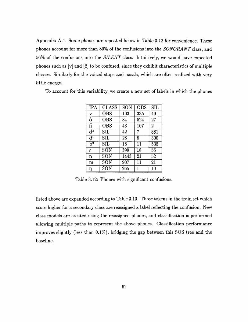
Appendix A.1. Some phones are repeated below in Table 3.12 for convenience. These
phones account for more than 80% of the confusions into the SONORANT class, and
56% of the confusions into the SILENT class. Intuitively, we would have expected
phones such as [v] and [6] to be confused, since they exhibit characteristics of multiple
classes. Similarly for the voiced stops and nasals, which are often realized with very
little energy.
To account for this variability, we create a new set of labels in which the phones
IPA CLASS SON OBS SILv OBS 103 335 496 OBS 84 524 27fi OBS 43 107 2d" SIL 42 7 881cf SIL 28 8 300bD SIL 18 11 535r SON 399 18 55n SON 1443 21 52m SON 907 11 21
u SON 265 1 10
Table 3.12: Phones with significant confusions.
listed above are expanded according to Table 3.13. Those tokens in the train set which
score higher for a secondary class are reassigned a label reflecting the confusion. New
class models are created using the reassigned phones, and classification is performed
allowing multiple paths to represent the above phones. Classification performance
improves slightly (less than 0.1%), bridging the gap between this SOS tree and the
baseline.

Original New labelsv v obs, vson, v sil6 6 obs, 6_son, &_silfi fobs, fison, isildD dDsil, dnson
' _ _ sil, psonbD b _sil, bPsonr rson, rsilm mrson, m.siln n-son, n-sil
0 r3-son, r.-sil
Table 3.13: Reassigned labels.
3.4 Chapter Summary
We have demonstrated that an MAP based hierarchical feature representation is a
feasible structure for classification, and that it can match the performance of the
baseline system when optimizations are performed on the features at each node.
Though scores for the unoptimized hierarchies are slightly below those of the baseline,
optimizing features at the individual nodes compensates for this initial drop. It
is encouraging to see this level of performance even with the use of crude feature
optimizations on a single node of the tree. More significant gains are to be expected
with the use of better feature optimization procedures.
In the next chapter, we see that a hierarchical structure offers a relatively risk-
free method for reducing computation. By pruning unlikely phonetic classes, we can
reduce the space of candidate phones, as well as the number of candidate words in
lexical access.

Chapter 4
Pruning
In the hierarchical framework, potentially complex decisions between confusable phones
are delayed while simpler, robust decisions based on general attributes are made at
the start. Since the hierarchy is structured in such a way, the probability scores ob-
tained for these initial stages are robust, as the scores in the previous section indicate.
This suggests that we can exploit the tree structure of the hierarchy and eliminate
branches of the tree following low scoring nodes. Since the classification accuracy
at the broad class level is bound to be much higher than that at the phone level,
we can be confident that most decisions will be correct. If more accurate decisions
are desired, the thresholds can be relaxed such that the correct path is almost never
eliminated.
The motivation behind a pruning strategy is twofold. First, because a hierarchy
requires broad class scores to be computed, in addition to individual phone scores,
it inevitably requires more computation at run-time than a single-pass scheme. This
means that the hierarchy will always be the slower approach. However, with prun-
ing, the effective size of the hierarchy can be decreased, so that speed is no longer
an issue. In fact, it will probably be the quicker of the two classification schemes.

Second, effective pruning allows a fastmatch at run-time, so that word candidates
can be reduced even as the phone is being classified. The benefits are in space (fewer
word hypotheses) as well as speed (fewer word matches can constrain the paths that
must be scored). We will study two different methods for establishing a pruning
threshold. First, we will prune all classes scoring below a fraction of the highest score.
If, for instance, the nasal class scores Pr(NASAL I f) = 0.6, and we choose to prune
at 50%, we will eliminate all classes scoring below 0.3. Second, we will prune all
classes below the n highest scoring classes. For this condition, we also examine the
likelihood that the correct class is within this n best threshold. The criteria we will
use for judging the effectiveness of the thresholds will be performance and computa-
tion reduction.
We will evaluate the pruning thresholds on the manner based tree of the pre-
vious chapter, since this tree was determined to be very similar in performance to
the baseline, achieving nearly the same classification accuracy at both the class and
phone levels. To isolate the effect of pruning from other considerations, we will use
the baseline feature vector for all experiments. We choose to prune on ly at the class
level in the two-stage Manner tree. For multiple level trees, where the classification
robustness varies at different levels of the tree, it may be necessary to vary the thresh-
old depending on the reliability of the node, in order to achieve a safe bound at each
decision point.
4.1 Results
Figure 4-1 shows classification accuracy as the pruning threshold is varied relative
to the highest scoring phonetic class. As the plateau in the graph indicates, classi-
fication accuracy is not affected until the threshold is set to within 60%-80% of the
maximum. The computational load, as a percentage of the baseline, is shown in Fig-
ure 4-2. Note that more than half the computation can be eliminated by setting the

Threshold with respect to maximum (%)
Figure 4-1: Classification accuracy with pruning
Threshold with respect to maximum (%)
Figure 4-2: Computation required, as percentage of baseline.
76.5
0
C.)
100

threshold to just 5% of the maximum. As we approach 0%, we are not rejecting any
of the paths, so computation is greater than that for the baseline, since we have an
additional 10% from the 6 class models as well as the 60 phone models. At the other
extreme, approaching 100%, we are only accepting the top choice path, so nearly 65%
of the computation is eliminated. For the plateau region of Figure 4-1, the compu-
tation remains steadily between 35% and 40% of the baseline. Therefore, by setting
the threshold safely at 5%, we can achieve roughly 60% reduction in computation
without loss of performance.
We can also observe performance and the corresponding reduction in computa-
tion as we prune the 6 - n worst candidates (or, alternatively, keep only the n best).
Overall classification accuracies as n is varied between 1 and 6 are shown in Figure
4-3. The scores at the two endpoints for the n = 1 case (top choice) and the n =
1 76.5
0
o
. 76.0
n1 2 3 4 5 6
Figure 4-3: Classification accuracy after pruning all but the n-best class models.
6 case (no pruning) match those of Figure 4-1, where 100% correponds to the top
choice and 0% corresponds to no pruning.
The computational savings associated with each of the pruning thresholds of Fig-

ure 4-3 are shown in Figure 4-4.
It is clear that there are no substantial savings in computation until the pruning
threshold is set to n = 2, which seems rather high. To investigate the feasibility of
this stringent threshold, we can observe the frequency of the correct class scoring
among the n best (Figure 4-5). These numbers are all high, but there is a distinct
jump in performance between n = 1 and n = 2. To be safe, we would like to place
the threshold further inside the plateau, as we did in the first case. Unfortunately,
this means a smaller savings in computation.
Comparing the two pruning methods, the first seems to offer more robust per-
formance at a greater computational savings, making it the better choice. In fact,
according to Figure 4-5, for the given conditions, we must prune all but the top choice
in order to match the computational savings offered by the first pruning strategy. We
would like to avoid this for obvious reasons.
One explanation why the n best method is less appealing may be that ranking the
models does not preserve a measure of absolute scores, so that models scoring near
zero, though they could reasonably be eliminated (and probably would be by the first
method), often climb to high standing when only one class model scores well. With
the first method, if only one class model scores well, it will be the only one considered.
4.2 Chapter Summary
The advantages and disadvantages of pruning are quite clear. Because unlikely phone
or class candidates can be eliminated robustly, we can achieve near baseline perfor-
mance with less than half of the computational load. However, because pruning
phonetic classes is equivalent to making a hard decision, doing so invariably results in
a loss of information. One consequence could be a less effective lexical access, which
weighs the scores of multiple phone candidates in arriving at an optimal phone string.
Despite this drawback, pruning is an attractive option available to the hierarchical

100
Figure 4-4: Computation required, as percentage of baseline
1 2 3 4 5 6
Figure 4-5: Inclusion of correct model within top n scores

framework. With a loosely set pruning threshold, a hierarchy could offer computa-
tional savings at a negligible risk. For more stringent thresholds, it might be feasible
to provide pruned phones with some minimum score, or assign these phones some
score that reflects the likelihood of the broad phonetic class to which they belong,
thereby maintaining some finite probability that the phone could have been spoken.

Chapter 5
Conclusions and Future Directions
5.1 Summary
In this thesis, we have attempted to assess the effectiveness of a hierarchical frame-
work for classifying speech sounds. We have developed tree structures based on
broad phonetic classes, and used an MAP probabilistic framework to score classes
and phones alike, at various stages in the tree. This framework has been motivated
by the desire to evaluate speech segments based on meaningful subsets of features,
in order to improve the robustness of the acoustic models and probability estimates.
A benefit of such a framework is that it allows the system to perform fine phonetic
distinctions, so that acoustically similar regions of confusable words can be inspected
with a greater level of specificity than dissimilar regions.
We have demonstrated that a modularized approach to classification is an appeal-
ing and potentially more robust framework for classification. Experimental results
have indicated that within the hierarchical framework, optimizing the features for a
given node will lead to improvements not only at that node but also overall. However,
further studies are necessary to see if the hierarchy can provide significantly better

performance than a one-shot classification.
We have also demonstrated that the ability to prune phonetic classes gives the
hierarchy a computational advantage over a uniform feature vector. We have shown
that with a well chosen threshold, significant savings in computation can be achieved
with absolutely no deterioration in performance. This suggests that with well chosen
features at each node in the hierarchy, better performance can be achieved at a re-
duced computational cost.
These results highlight two driving forces behind the hierarchy. The first is the
ability to isolate fine phonetic distinctions from broader ones, enabling the use of
heterogeneous feature sets for optimally discriminating among sounds of differing
acoustic significance. The second is the potential for fastmatch, which can focus the
search space on a probable subset of candidate words. For the latter purpose, the
hierarchy can be designed to balance good acoustic classes with classes that facilitate
lexical access.
5.2 Future Directions
Several avenues remain to be explored. We have only developed hierarchies manually,
using an intuitive choice of phonetic classes and a crude optimization on the features.
Immediate improvements can be made using an automatic procedure for selecting
features for each phonetic decision. SAILS offers one way to accomplish this.
SAILS has been developed within the Spoken Language Systems group to allow
for the automatic optimisation of feature parameters across a specified set of tokens
[19, 21]. It relies on the speech scientist to provide meaningful attributes for a given
class of sounds, and optimises the parameters to best discriminate among the sounds.
We could, for instance, use SAILS to search for the optimal time bounds within a
speech segment to discriminate among the stops. In this case SAILS would likely

verify that the beginning of the segment is where we should extract measurements.
Recently, SAILS has been enhanced to select the optimal subset of features for mak-
ing a particular phonetic distinction. Applying such a procedure to the various nodes
in a hierarchy would be one step toward fully utilizing the flexibility afforded by the
hierarchy.
For optimal performance, an iterative approach to selecting both features and
classes might be worth investigating. We can propose a few phonetic classes as part
of a hierarchy, and then find features for optimally discriminating among them. We
can then reassign the classes based on confusion (allowing for phones to belong to
multiple classes), and again optimize the features for these new classes. In time, the
feature sets should gradually become more compact at each node, and the phonetic
classes more homogeneous. Similarly, we can begin by first hypothesizing a set of
features, and automatically determine an initial scattering of phonetic classes based
on those features.
Eventually, it may be desirable to incorporate more context dependent units into
the hierarchy. This could be in the form of context dependent phones, or even syl-
lables. For a context dependent hierarchy, each context indpendent phone model in
the current scheme could be replaced by several context dependent models, without
the need for major revisions to the structure presented in this thesis. Heterogeneous
feature sets could be used for differing contexts.
It should be noted that the use of heterogeneous feature sets could include the use
of features derived from different signal representations. With the baseline window
size and frame rate, many acoustic cues, such as the [b] plosive, which often last on
the order of 10 ms, will be smoothed over or contain acoustic information from neigh-
boring regions of the waveform. Other representations are worth considering for this
reason. A wavelet representation, or a representation derived from a shorter analysis
window would be ideal for capturing localized events in the waveform, and could be
incorporated into a hierarchical framework at nodes requiring temporal information.

Finally, based on the results of the pruning study, and the feasibility of the hierar-
chical framework we have proposed in this thesis, it might be desirable to implement
a hybrid lexical search, in which phones or classes could be hypothesized to form
the elements of the lexical string. This would enable all elements of the string to
maintain a minimum level of confidence. After all, it could be argued that a phone
with an exceedingly low score conveys no useful information, even if it represents the
highest score among the phone set. The classifier could back off when it encountered
an unrecognizable segment and instead hypothesize NASAL, as opposed to [m] or [n].
This is possible within the hierarchical framework because the classifier assigns prob-
ability scores to all nodes in the hierarchy, at both a coarse and fine level, reflecting
the varying degrees of certainty and significance in the structure of speech sounds.

Appendix A
Confusion Statistics
A.1 SONORANT vs. OBSTRUENT vs. SILENT
partition

SON OBS SIL SON OBS SILa 610 0 0 I 993 1 0ae 535 0 0 i 1736 8 0A 612 0 0 i 1244 2 0a 538 0 0 J 0 209 0
w" 155 0 0 k 1 824 3a 945 7 3 k0 5 5 9333h 51 14 12 1 1293 13 6a 710 3 4 m 907 11 21oY 472 0 0 n 1443 21 52b 6 628 3 U 265 1 10b" 18 11 535 ? 169 1 2
1 0 195 0 o 432 0 0d 4 591 7 cD 97 0 0do 42 7 881 p 1 674 1
6 84 524 27 o 11 5 248r 399 18 55 p0 1 5 685E 855 1 0 r 1290 14 21 241 0 1 s 0 1510 1
m 30 0 2 S 0 326 0n 149 1 5 t 0 942 12
U 4 0 0 t' 25 13 13500 7 20 199 0 0 169 14
3 461 0 0 0 161 0 0e 571 0 1 u 108 0 1f 0 618 13 ii 299 0 0g 6 315 4 v 103 335 49g0 28 7 300 w 608 11 5h# 3 3 1882 y 253 8 0h 3 224 8 z 2 869 3
i 43 107 2 2 0 54 0
Table A.1: Phone confusions

Bibliography
[1] Rolf Carlson and James R. Glass "Vowel Classification Based on Analysis-by-
Synthesis," In Proceedings of the 1992 Conference on Spoken Language Process-
ing, 1992.
[2] Ronald A. Cole, Richard M. Stern, and Moshe J. Lasry. "Performing Fine Pho-
netic Distinctions: Templates versus Features," In J.S. Perkell and D.M. Klatt,
editors, Variability and Invariance in Speech Processes. Lawrence Erlbaum As-
soc., 1986.
[3] Richard O. Duda and Peter E. Hart. Pattern Classification and Scene Analysis.
John Wiley and Sons, 1973.
[4] G. Fant. Acoustic Theory of Speech Production. Mouton and Co., The Hague,
Netherlands, 1960.
[5] James R. Glass "Nasalized Consonants and Nasalized Vowels: An Acoustic Study
and Recognition Experiment," S.M. Thesis, Department of Electrical Engineer-
ing and Compute Science, Massachusetts Institute of Technology, December,
1984.
[6] William D. Goldenthal "Statistical Trajectory Models for Phonetic Recognition,"
Ph.D. Thesis, Department of Aeronautics and Astronautics, Massachusetts Insi-
titute of Technology, September, 1994.

[7] David B. Grayden and Michael S. Scordilis. "Recognition of Obstruent Phonemes
in Speaker-Independent Speech Using a Hierarchical Approach," In Proceedings
of the 1993 EUROSPEECH, 855-858, 1993.
[8] David B. Grayden and Michael S. Scordilis. "Phonemic Segmentation of Fluent
Speech," In Proceedings of the 1994 International Conference on Acoustics,
Speech, and Signal Processing, 73-77. IEEE, 1994.
[9] Daniel P. Huttenlocher and Victor W. Zue. "A Model of Lexical Access From
Partial Information," Ph.D. Thesis, Massachusetts Institute of Technology, June,
1985.
[10] Lori F. Lamel and J. L. Gauvain. "High Performance Speaker-Independent Phone
Recognition Using CDHMM," In Proceedings of the 1993 EUROSPEECH, 121-
124, 1993.
[11] Lori F. Lamel, Robert H. Kassel, and Stephanie S. Seneff. "Speech Database
Development: Design and Analysis of the Acoustic-Phonetic Corpus," In Pro-
ceedings of the DARPA Speech Recognition Workshop, Report No. SAIC-86/1546,
February, 1986.
[12] K.F. Lee. "Large-Vocabulary Speaker-Independent Continuous Speech Recog-
nition: The SPHINX System," Ph.D. Thesis, Computer Science Department,
Carnegie Mellon Univ., 1988
[13] Hong C. Leung, Benjamin Chigier, and James R. Glass. "A Comparative Study
of Signal Representations and Classification Techniques for Speech Recognition,"
Proc. ICASSP 93, 680-683, Minneapolis, MN, April, 1993.
[14] Hong C. Leung "The Use of Artificial Neural Nets for Phonetic Recognition,"
Ph.D. Thesis, Department of Electrical Engineering and Computer Science, Mas-
sachusetts Institute of Technology, May, 1989.

[15] Hong C. Leung and Victor W. Zue. "A Procedure for Automatic Alignment of
Phonetic Transcriptions with Continuous Speech," S.M. Thesis, Massachusetts
Institute of Technology, January, 1985.
[16] Helen M. Meng and Victor W. Zue. "The Use of Distinctive Features for Auto-
matic Speech Recognition," S.M. Thesis, Massachusetts Institute of Technology,
June, 1991.
[17] P. Mermelstein and S. Davis. "Comparison of Parametric Representations for
Monosyllabic Word Recognition in Continuosly Spoken Sentences," IEEE Trans-
actions on Acoustics, Speech, and Signal Processing, vol. ASSP-28, No. 4, August
1980.
[18] G.A. Miller and P.E. Nicely. "An Analysis of Perceptual Confusions Among Some
English Consonants," Journal of the Acoustical Society of America, Vol.24, No.2,
1954.
[19] Manish Muzumdar and Lee Hetherington. Personal communication regarding
development of SAILS.
[20] G.E. Peterson and H.L Barney. "Control Methods Used in a Study of the Vow-
els," Journal of the Acoustical Society of America, 175-194, March, 1952.
[21] Mike Phillips. "Automatic Discovery of Acoustic Measurements for Phonetic
Classification," J. Acoust. Soc. Am., vol. 84, S216, 1988.
[22] Mike Phillips, James R. Glass, Victor W. Zue. "Automatic Learning of Lexical
Representations for Sub-Word Unit Based Speech Recognition Systems," In
Proc. of the 1991 EUROSPEECH, 577-580, Genova, Italy, September, 1991.
[23] Lawrence R. Rabiner and Biing-Hwang Juang. Fundamentals of Speech Recog-
nition Prentice Hall, 1993.

[24] Lawrence R. Rabiner and R.W. Shafer. Digital Processing of Speech Signals
Prentice Hall, 1978.
[25] "A Computational Model for the Peripheral Auditory System: Application to
Speech Recognition Research," In Proc. ICASSP 86, Tokyo, 1986.
[26] David W. Shipman and Victor W. Zue. "Properties of Large Lexicons: Impli-
cations for Advanced Isolated Word Recognition Systems," In Proceedings of
the 1982 International Conference on Acoustics, Speech, and Signal Processing,
546-549. IEEE, 1982.
[27] Kenneth N. Stevens. "Phonetic Evidence for Hierarchies of Features," In P.
Keating (ed.) Phonological Structure and Phonetic Form: Papers in Laboratory
Phonology III, 242-258, Cambridge Univ. Press, 1994.
[28] Victor W. Zue. "The Use of Speech Knowledge in Automatic Speech Recogni-
tion," In Proceedings of the IEEE, vol. 73, 1602-15, November 1985.
[29] Victor W. Zue and R.A. Cole. "Experiments on Spectrogram Reading," in Pro-
ceedings of the 1979 International Conference on Acoustics, Speech, and Signal
Processing, 116-119, 1979.
[30] Victor W. Zue, James R. Glass, Mike Phillips, and Stephanie S. Seneff. "Acous-
tic Segmentation and Phonetic Classification in the SUMMIT System," In Pro-
ceedings of the 1989 International Conference on Acoustics, Speech, and Signal
Processing, 389-392. IEEE, 1989.