a guide to approximationsnnp.ucsd.edu/phy120b/student_dirs/shared/gnarly/misc_docs/trig... · this...

A Guide to Approximations

Jack G. Ganssle

[email protected]

The Ganssle Group PO Box 38346

Baltimore, MD 21231 (410) 496-3647

fax (410) 675-2245

Jack Ganssle believes that embedded development can be much more efficient than it usually is, and that we can – and must – create more reliable products. He conducts one-day seminars that teach ways to produce better firmware faster. For more information see www.ganssle.com.

© 2001 The Ganssle Group. This work may be used by individuals and companies, but all publication rights reserved.

Floating Point Approximations Most embedded processors don’t know how to compute trig and other complex functions. Programming in C we’re content to call a library routine that does all of the work for us. Unhappily this optimistic approach often fails in real time systems where size, speed and accuracy are all important issues. The compiler’s runtime package is a one-size-fits-all proposition. It gives a reasonable trade-off of speed and precision. But every embedded system is different, with different requirements. In some cases it makes sense to write our own approximation routines. Why?

Speed – Many compilers have very slow runtime packages. A clever approximation may eliminate the need to use a faster CPU. Predictability – Compiler functions vary greatly in execution time depending on the input argument. Real time systems must be predictable in the time domain. The alternative is to always assume worst case execution time, which again may mean your CPU is too slow, too loaded, for the application. Accuracy – Read the compiler’s manuals carefully! Some explicitly do not support the ASNI C standard, which requires all trig to be double precision. (8051 compilers are notorious for this). Alternatively, why pay the cost (in time) for double precision math when you only need 5 digits of accuracy? Size – When memory is scarce, using one of these approximations may save much code space. If you only need a simple cosine, why include the entire floating point trig library?

This collection is not an encyclopedia of all possible approximations; rather, it’s the most practical ones distilled from the bible of the subject, Computer Approximations by John Hart (ISBN 0-88275-642-7). Unfortunately this work is now out of print. It’s also very difficult to use without a rigorous mathematical background. All of the approximations here are polynomials, or ratios of polynomials. All use very cryptic coefficients derived from Chebyshev series and Bessel functions. Rest assured that these numbers give minimum errors for the indicated ranges. Each approximation (with a few exceptions) has an error cha rt so you can see exactly where the errors occur. In some cases, if you’re using a limited range of input data, your accuracies can far exceed the indicated values. For instance, cos_73 is accurate to 7.3 decimal digits over the 0 to 360 degree range. But as the graph shows, in the range 0 to 30 degrees you can get almost an order of magnitude improvement.


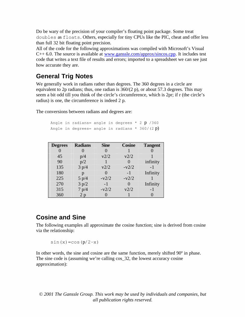
Do be wary of the precision of your compiler’s floating point package. Some treat doubles as floats. Others, especially for tiny CPUs like the PIC, cheat and offer less than full 32 bit floating point precision. All of the code for the following approximations was compiled with Microsoft’s Visual C++ 6.0. The source is available at www.ganssle.com/approx/sincos.cpp. It includes test code that writes a text file of results and errors; imported to a spreadsheet we can see just how accurate they are.

General Trig Notes We generally work in radians rather than degrees. The 360 degrees in a circle are equivalent to 2p radians; thus, one radian is 360/(2 p), or about 57.3 degrees. This may seem a bit odd till you think of the circle’s circumference, which is 2pr; if r (the circle’s radius) is one, the circumference is indeed 2 p. The conversions between radians and degrees are:

Angle in radians= angle in degrees * 2 p /360 Angle in degrees= angle in radians * 360/(2 p)

Degrees Radians Sine Cosine Tangent

0 0 0 1 0 45 p/4 v2/2 v2/2 1 90 p/2 1 0 infinity 135 3 p/4 v2/2 -v2/2 -1 180 p 0 -1 Infinity 225 5 p/4 -v2/2 -v2/2 1 270 3 p/2 -1 0 Infinity 315 7 p/4 -v2/2 v2/2 -1 360 2 p 0 1 0

Cosine and Sine The following examples all approximate the cosine function; sine is derived from cosine via the relationship:

sin(x)=cos(p/2-x)

In other words, the sine and cosine are the same function, merely shifted 90º in phase. The sine code is (assuming we’re calling cos_32, the lowest accuracy cosine approximation):


All of the cosine approximations in this chapter compute the cosine accurately over the range of 0 to p/2 (0 to 90º). That surely denies us of most of the circle! Approximations in general work best over rather limited ranges; it’s up to us to reduce the input range to something the approximation can handle accurately. Therefore, before calling any of the following cosine approximations we assume the range has been reduced to 0 to p/2 using the following code:

This code is configured to call cos_32s, which is the approximation (detailed shortly) for computing the cosine to 3.2 digits accuracy. Use this same code, though, for all cosine approximations; change cos_32s to cos_52s, cos_73s or cos_121s, depending on which level of accuracy you need. See the complete listing for a comprehensive example. If you can guarantee that the input argument will be greater than zero and less than 2 p, delete the two red lines in the listing above to get even faster execution. Be clever about declaring variables and constants. Clearly, working with the cos_32 approximation nothing must be declared “double”. Use float for more efficient code.

// Math constants double const pi=3.1415926535897932384626433;// pi double const twopi=2.0*pi; // pi times 2 double const halfpi=pi/2.0; // pi divided by 2 // // This is the main cosine approximation "driver" // It reduces the input argument's range to [0, pi/2], // and then calls the approximator. // float cos_32(float x){ int quad; // what quadrant are we in? x=fmod(x, twopi); // Get rid of values > 2* pi if(x<0)x=-x; // cos(-x) = cos(x) quad=int(x/halfpi); // Get quadrant # (0 to 3) switch (quad){ case 0: return cos_32s(x); case 1: return -cos_32s(pi-x); case 2: return -cos_32s(x-pi); case 3: return cos_32s(twopi-x); } }

// The sine is just cosine shifted a half-pi, so // we'll adjust the argument and call the cosine approximation. // float sin_32(float x){ return cos_32(halfpi-x); }


Reading the complete listing you’ll notice that for cos_32 and cos_52 we used floats everywhere; the more accurate approximations declare things as doubles. One trick that will speed up the approximations is to compute x2 by incrementing the characteristic of the floating point representation of x. You’ll have to know exactly how the numbers are stored, but can save hundreds of microseconds over performing the much clearer “x*x” operation. How does the range reduction work? Note that the code divides the input argument into one of four “quadrants” – the very same quadrants of the circle shown below:

Quadrants 0 to 3 of the circle

• For the first quadrant (0 to p/2) there’s nothing to do since the cosine approximations are valid over this range.

• In quadrant 1 the cosine is symertrical with quadrant 0, if we reduce it’s range by subtracting the argument from p. The cosine, though, is negative for quadrants 1 and 2 so we compute –cos(p-x).

• Quadrant 2 is similar to 1. • Finally, in 3 the cosine goes positive again; if we subtract the argument from 2 p

it translates back to something between 0 and p/2. The approximations do convert the basic polynomial to a simpler, much less computationally expensive form, as described in the comments. All floating point operations take appreciable amounts of time, so it’s important to optimize the design.

0

p/2

p

3p/2

0

3

1

2


cos_32 & sin_32 absolute error

-1

-0.8

-0.6

-0.4

-0.2

0

0.2

0.4

0.6

0.8

1

0 30 60 90 120 150 180 210 240 270 300 330 360Degrees

cos(

x)

-0.0006

-0.0004

-0.0002

0

0.0002

0.0004

0.0006

Err

or

cos(x) cos_32 error sin_32 error

cos_32 computes a cosine to about 3.2 decimal digits of accuracy. Use the range reduction code (listed earlier) if the range exceeds 0 to p/2. The plotted errors are absolute (not percent error).

// cos_32s computes cosine (x) // // Accurate to about 3.2 decimal digits over the range [0, pi/2]. // The input argument is in radians. // // Algorithm: // cos(x)= c1 + c2*x**2 + c3*x**4 // which is the same as: // cos(x)= c1 + x**2(c2 + c3*x**2) // float cos_32s(float x) { const float c1= 0.99940307; const float c2=-0.49558072; const float c3= 0.03679168; float x2; // The input argument squared x2=x * x; return (c1 + x2*(c2 + c3 * x2)); }



-1

-0.8

-0.6

-0.4

-0.2

0

0.2

0.4

0.6

0.8

1

0 30 60 90 120 150 180 210 240 270 300 330 360Degrees

cos(

x)

-8.0E-06

-6.0E-06

-4.0E-06

-2.0E-06

0.0E+00

2.0E-06

4.0E-06

6.0E-06

8.0E-06

Err

or

cos(x) cos_52 Error sin_52 Error

cos_52 computes a cosine to about 5.2 decimal digits of accuracy. Use the range reduction code (listed earlier) if the range exceeds 0 to p/2. The plotted errors are absolute (not percent error).

// cos_52s computes cosine (x) // // Accurate to about 5.2 decimal digits over the range [0, pi/2]. // The input argument is in radians. // // Algorithm: // cos(x)= c1 + c2*x**2 + c3*x**4 + c4*x**6 // which is the same as: // cos(x)= c1 + x**2(c2 + c3*x**2 + c4*x**4) // cos(x)= c1 + x**2(c2 + x**2(c3 + c4*x**2)) // float cos_52s(float x) { const float c1= 0.9999932946; const float c2=-0.4999124376; const float c3= 0.0414877472; const float c4=-0.0012712095; float x2; // The input argument squared x2=x * x; return (c1 + x2*(c2 + x2*(c3 + c4*x2))); }



-1

-0.8

-0.6

-0.4

-0.2

0

0.2

0.4

0.6

0.8

1

0 30 60 90 120 150 180 210 240 270 300 330 360Degrees

cos(

x)

-3.0E-06

-2.0E-06

-1.0E-06

0.0E+00

1.0E-06

2.0E-06

3.0E-06

Err

or


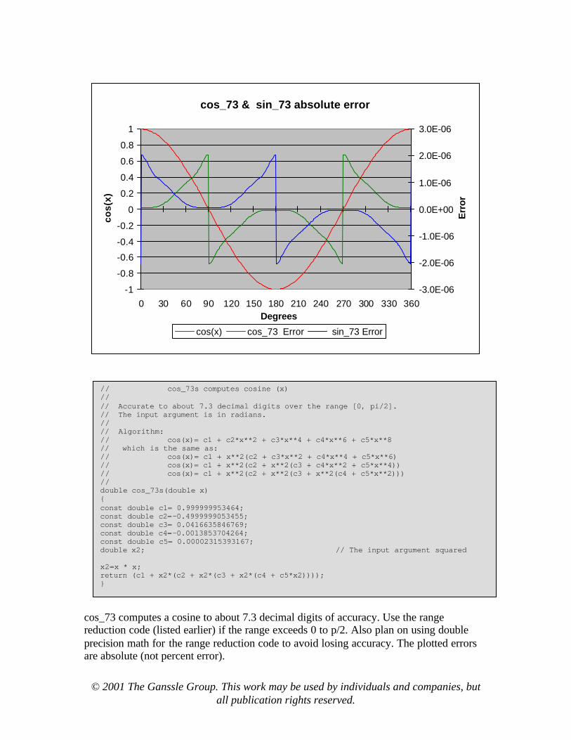
cos_73 computes a cosine to about 7.3 decimal digits of accuracy. Use the range reduction code (listed earlier) if the range exceeds 0 to p/2. Also plan on using double precision math for the range reduction code to avoid losing accuracy. The plotted errors are absolute (not percent error).

// cos_73s computes cosine (x) // // Accurate to about 7.3 decimal digits over the range [0, pi/2]. // The input argument is in radians. // // Algorithm: // cos(x)= c1 + c2*x**2 + c3*x**4 + c4*x**6 + c5*x**8 // which is the same as: // cos(x)= c1 + x**2(c2 + c3*x**2 + c4*x**4 + c5*x**6) // cos(x)= c1 + x**2(c2 + x**2(c3 + c4*x**2 + c5*x**4)) // cos(x)= c1 + x**2(c2 + x**2(c3 + x**2(c4 + c5*x**2))) // double cos_73s(double x) { const double c1= 0.999999953464; const double c2=-0.4999999053455; const double c3= 0.0416635846769; const double c4=-0.0013853704264; const double c5= 0.00002315393167; double x2; // The input argument squared x2=x * x; return (c1 + x2*(c2 + x2*(c3 + x2*(c4 + c5*x2)))); }



-1

-0.8

-0.6

-0.4

-0.2

0

0.2

0.4

0.6

0.8

1

0 30 60 90 120 150 180 210 240 270 300 330 360Degrees

cos(

x)

-1.2E-12

-8.0E-13

-4.0E-13

0.0E+00

4.0E-13

8.0E-13

1.2E-12

Err

or


cos_121 computes a cosine to about 12.1 decimal digits of accuracy. Use the range reduction code (listed earlier) if the range exceeds 0 to p/2. Also plan on using double

// cos_121s computes cosine (x) // // Accurate to about 12.1 decimal digits over the range [0, pi/2]. // The input argument is in radians. // // Algorithm: // cos(x)= c1+c2*x**2+c3*x**4+c4*x**6+c5*x**8+c6*x**10+c7*x**12 // which is the same as: // cos(x)= c1+x**2(c2+c3*x**2+c4*x**4+c5*x**6+c6*x**8+c7*x**10) // cos(x)= c1+x**2(c2+x**2(c3+c4*x**2+c5*x**4+c6*x**6+c7*x**8 )) // cos(x)= c1+x**2(c2+x**2(c3+x**2(c4+c5*x**2+c6*x**4+c7*x**6 ))) // cos(x)= c1+x**2(c2+x**2(c3+x**2(c4+x**2(c5+c6*x**2+c7*x**4 )))) // cos(x)= c1+x**2(c2+x**2(c3+x**2(c4+x**2(c5+x**2(c6+c7*x**2 ))))) // double cos_121s(double x) { const double c1= 0.99999999999925182; const double c2=-0.49999999997024012; const double c3= 0.041666666473384543; const double c4=-0.001388888418000423; const double c5= 0.0000248010406484558; const double c6=-0.0000002752469638432; const double c7= 0.0000000019907856854; double x2; // The input argument squared x2=x * x; return (c1 + x2*(c2 + x2*(c3 + x2*(c4 + x2*(c5 + x2*(c6 + c7*x2)))))); }


precision math for the range reduction code to avoid losing accuracy. The plotted errors are absolute (not percent error).

Higher Precision Cosines Given a large enough polynomial there’s no limit to the possible accuracy. A few more algorithms are listed here. These are all valid for the range of 0 to p/2, and all can use the previous range reduction algorithm to change any angle into one within this range. All take an input argument in radians. No graphs are included because these exceed the accuracy of the typical compiler’s built-in cosine function… so there’s nothing to plot the data against. Note that C’s double type on most computers carries about 15 digits of precision. So for these algorithms, especially for the 20.2 and 23.1 digit versions, you’ll need to use a data type that offers more bits. Some C’s support a long double. But check the manual carefully! Microsoft’s Visual C++, for instance, while it does support the long double keyword, converts all of these to double. Accurate to about 14.7 decimal digits over the range [0, p/2]:

c1= 0.99999999999999806767 c2=-0.4999999999998996568 c3= 0.04166666666581174292 c4=-0.001388888886113613522 c5= 0.000024801582876042427 c6=-0.0000002755693576863181 c7= 0.0000000020858327958707 c8=-0.000000000011080716368 cos(x)= c1 + x2(c2 + x2(c3 + x2(c4 + x2(c5 +

x2(c6 + x2(c7 + x2*c8)))))) Accurate to about 20.2 decimal digits over the range [0, p/2]:

c1 = 0.9999999999999999999936329 c2 =-0.49999999999999999948362843 c3 = 0.04166666666666665975670054 c4 =-0.00138888888888885302082298 c5 = 0.000024801587301492746422297 c6 =-0.00000027557319209666748555 c7 = 0.0000000020876755667423458605 c8 =-0.0000000000114706701991777771 c9 = 0.0000000000000477687298095717 c10=-0.00000000000000015119893746887 cos(x)= c1 + x2(c2 + x2(c3 + x2(c4 + x2(c5 + x2(c6 +

x2(c7 + x2(c8 + x2(c9 + x2*c10)))))))) Accurate to about 23.1 decimal digits over the range [0, p/2]:

c1 = 0.9999999999999999999999914771 c2 =-0.4999999999999999999991637437 c3 = 0.04166666666666666665319411988 c4 =-0.00138888888888888880310186415 c5 = 0.00002480158730158702330045157 c6 =-0.000000275573192239332256421489


c7 = 0.000000002087675698165412591559 c8 =-0.0000000000114707451267755432394 c9 = 0.0000000000000477945439406649917 c10=-0.00000000000000015612263428827781 c11= 0.00000000000000000039912654507924 cos(x)= c1 + x2(c2 + x2(c3 + x2(c4 + x2(c5 + x2(c6 +

x2(c7 + x2(c8 + x2(c9 + x2(c10 + x2*c11)))))))))


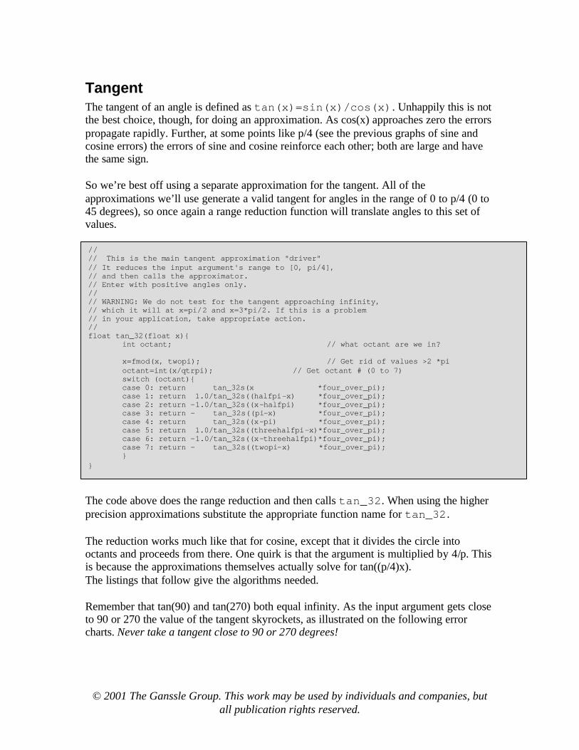
Tangent The tangent of an angle is defined as tan(x)=sin(x)/cos(x). Unhappily this is not the best choice, though, for doing an approximation. As cos(x) approaches zero the errors propagate rapidly. Further, at some points like p/4 (see the previous graphs of sine and cosine errors) the errors of sine and cosine reinforce each other; both are large and have the same sign. So we’re best off using a separate approximation for the tangent. All of the approximations we’ll use generate a valid tangent for angles in the range of 0 to p/4 (0 to 45 degrees), so once again a range reduction function will translate angles to this set of values.

The code above does the range reduction and then calls tan_32. When using the higher precision approximations substitute the appropriate function name for tan_32. The reduction works much like that for cosine, except that it divides the circle into octants and proceeds from there. One quirk is that the argument is multiplied by 4/p. This is because the approximations themselves actually solve for tan((p/4)x). The listings that follow give the algorithms needed. Remember that tan(90) and tan(270) both equal infinity. As the input argument gets close to 90 or 270 the value of the tangent skyrockets, as illustrated on the following error charts. Never take a tangent close to 90 or 270 degrees!

// // This is the main tangent approximation "driver" // It reduces the input argument's range to [0, pi/4], // and then calls the approximator. // Enter with positive angles only. // // WARNING: We do not test for the tangent approaching infinity, // which it will at x=pi/2 and x=3*pi/2. If this is a problem // in your application, take appropriate action. // float tan_32(float x){ int octant; // what octant are we in? x=fmod(x, twopi); // Get rid of values >2 *pi octant=int(x/qtrpi); // Get octant # (0 to 7) switch (octant){ case 0: return tan_32s(x *four_over_pi); case 1: return 1.0/tan_32s((halfpi-x) *four_over_pi); case 2: return -1.0/tan_32s((x-halfpi) *four_over_pi); case 3: return - tan_32s((pi-x) *four_over_pi); case 4: return tan_32s((x-pi) *four_over_pi); case 5: return 1.0/tan_32s((threehalfpi-x)*four_over_pi); case 6: return -1.0/tan_32s((x-threehalfpi)*four_over_pi); case 7: return - tan_32s((twopi-x) *four_over_pi); } }


tan_32 percentage error

-10

-8

-6

-4

-2

0

2

4

6

8

10

0 30 60 90 120 150 180 210 240 270 300 330 360Degrees

tan

(x)

-0.4

-0.3

-0.2

-0.1

0

0.1

0.2

0.3

0.4

Per

cen

t E

rro

r

tan(x) tan_32 % error

tan_32 computes the tangent of p/4*x to about 3.2 digits of accuracy. Use the range reduction code to trans late the argument to 0 to p/4, and of course to compensate for the peculiar “p/4” bias required by this routine. Note that the graphed errors are percentage error, not absolute.

// ********************************************************* // *** // *** Routines to compute tangent to 3.2 digits // *** of accuracy. // *** // ********************************************************* // // tan_32s computes tan(pi*x/4) // // Accurate to about 3.2 decimal digits over the range [0, pi/4]. // The input argument is in radians. Note that the function // computes tan(pi*x/4), NOT tan(x); it's up to the range // reduction algorithm that calls this to scale things properly. // // Algorithm: // tan(x)= x*c1/(c2 + x**2) // float tan_32s(float x) { const float c1=-3.6112171; const float c2=-4.6133253; float x2; // The input argument squared x2=x * x; return (x*c1/(c2 + x2)); }



-10

-8

-6

-4

-2

0

2

4

6

8

10

0 30 60 90 120 150 180 210 240 270 300 330 360Degrees

tan

(x)

-0.003

-0.002

-0.001

0

0.001

0.002

0.003

Per

cen

t E

rro

r


tan_56 computes the tangent of p/4*x to about 5.6 digits of accuracy. Use the range reduction code to translate the argument to 0 to p/4, and of course to compensate for the peculiar “p/4” bias required by this routine. Note that the graphed errors are percentage error, not absolute.

// ********************************************************* // *** // *** Routines to compute tangent to 5.6 digits // *** of accuracy. // *** // ********************************************************* // // tan_56s computes tan(pi*x/4) // // Accurate to about 5.6 decimal digits over the range [0, pi/4]. // The input argument is in radians. Note that the function // computes tan(pi*x/4), NOT tan(x); it's up to the range // reduction algorithm that calls this to scale things properly. // // Algorithm: // tan(x)= x(c1 + c2*x**2)/(c3 + x**2) // float tan_56s(float x) { const float c1=-3.16783027; const float c2= 0.134516124; const float c3=-4.033321984; float x2; // The input argument squared x2=x * x; return (x*(c1 + c2 * x2)/(c3 + x2)); }



-10-8

-6

-4-2

02

46

810

0 30 60 90 120 150 180 210 240 270 300 330 360Degrees

tan

(x)

-3.0E-06

-2.0E-06

-1.0E-06

0.0E+00

1.0E-06

2.0E-06

3.0E-06

Per

cen

t E

rro

r


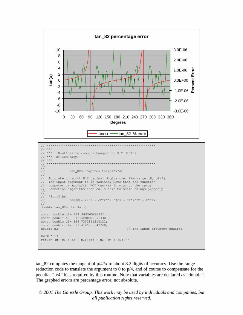
tan_82 computes the tangent of p/4*x to about 8.2 digits of accuracy. Use the range reduction code to translate the argument to 0 to p/4, and of course to compensate for the peculiar “p/4” bias required by this routine. Note that variables are declared as “double”. The graphed errors are percentage error, not absolute.

// ********************************************************* // *** // *** Routines to compute tangent to 8.2 digits // *** of accuracy. // *** // ********************************************************* // // tan_82s computes tan(pi*x/4) // // Accurate to about 8.2 decimal digits over the range [0, pi/4]. // The input argument is in radians. Note that the function // computes tan(pi*x/4), NOT tan(x); it's up to the range // reduction algorithm that calls this to scale things properly. // // Algorithm: // tan(x)= x(c1 + c2*x**2)/(c3 + c4*x**2 + x**4) // double tan_82s(double x) { const double c1= 211.849369664121; const double c2=- 12.5288887278448 ; const double c3= 269.7350131214121; const double c4=- 71.4145309347748; double x2; // The input argument squared x2=x * x; return (x*(c1 + c2 * x2)/(c3 + x2*(c4 + x2))); }



-10

-8

-6

-4

-2

0

2

4

6

8

10

0 30 60 90 120 150 180 210 240 270 300 330 360Degrees

tan

(x)

-1.0E-11

-7.0E-12

-4.0E-12

-1.0E-12

2.0E-12

5.0E-12

8.0E-12

Per

cen

t E

rro

r


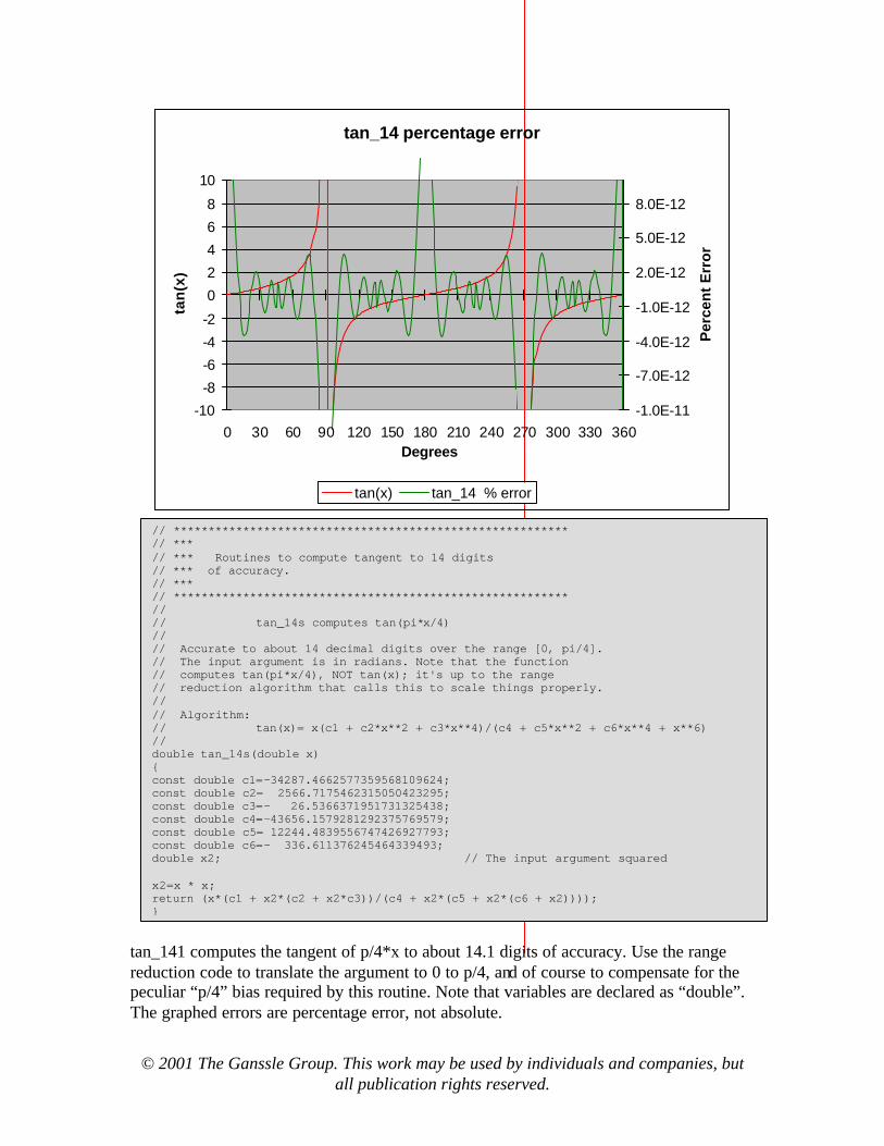
tan_141 computes the tangent of p/4*x to about 14.1 digits of accuracy. Use the range reduction code to translate the argument to 0 to p/4, and of course to compensate for the peculiar “p/4” bias required by this routine. Note that variables are declared as “double”. The graphed errors are percentage error, not absolute.

// ********************************************************* // *** // *** Routines to compute tangent to 14 digits // *** of accuracy. // *** // ********************************************************* // // tan_14s computes tan(pi*x/4) // // Accurate to about 14 decimal digits over the range [0, pi/4]. // The input argument is in radians. Note that the function // computes tan(pi*x/4), NOT tan(x); it's up to the range // reduction algorithm that calls this to scale things properly. // // Algorithm: // tan(x)= x(c1 + c2*x**2 + c3*x**4)/(c4 + c5*x**2 + c6*x**4 + x**6) // double tan_14s(double x) { const double c1=-34287.4662577359568109624; const double c2= 2566.7175462315050423295; const double c3=- 26.5366371951731325438; const double c4=-43656.1579281292375769579; const double c5= 12244.4839556747426927793; const double c6=- 336.611376245464339493; double x2; // The input argument squared x2=x * x; return (x*(c1 + x2*(c2 + x2*c3))/(c4 + x2*(c5 + x2*(c6 + x2)))); }


Higher Precision Tangents Given a large enough polynomial there’s no limit to the possible accuracy. A few more algorithms are listed here. These are all valid for the range of 0 to p/4, and all should use the previous range reduction algorithm to change any angle into one within this range. All take an input argument in radians, though it is expected to be mangled by the p/4 factor. The prior range reducer will correct for this. No graphs are included because these exceed the accuracy of the typical compiler’s built-in cosine function… so there’s nothing to plot the data against. Note that C’s double type on most computers carries about 15 digits of precision. So for these algorithms, especially for the 20.2 and 23.1 digit versions, you’ll need to use a data type that offers more bits. Some C’s support a long double. But check the manual carefully! Microsoft’s Visual C++, for instance, while it does support the long double keyword, converts all of these to double. Accurate to about 20.3 digits over the range of 0 to p/4:

c1= 10881241.46289544215469695742 c2=- 895306.0870564145957447087575 c2= 14181.99563014366386894487566 c3=- 45.63638305432707847378129653 c4= 13854426.92637036839270054048 c5=- 3988641.468163077300701338784 c6= 135299.4744550023680867559195 c7=- 1014.19757617656429288596025 tan(xp/4)=x(c1 + x2(c2 + x2(c3 + x2*c4)))

/(c5 + x2(c6 + x2(c7 + x2))) Accurate to about 23.6 digits over the range of 0 to p/4:

c1= 4130240.558996024013440146267 c2=- 349781.8562517381616631012487 c3= 6170.317758142494245331944348 c4=- 27.94920941480194872760036319 c5= 0.0175143807040383602666563058 c6= 5258785.647179987798541780825 c7=-1526650.549072940686776259893 c8= 54962.51616062905361152230566 c9=- 497.495460280917265024506937 tan(xp/4)=x(c1 + x2(c2 + x2(c3 + x2(c4 + x2*c5))))

/(c6 + x2(c7 + x2(c8 + x2(c9 + x2))))


Arctangent, arcsine and arccosine The arctangent is the same as the inverse tangent, so arctan(tan(x))=x. It’s often denoted as “atan(x)” or “tan-1(x)”. In practice the approximations for inverse sine an cosine aren’t too useful; mostly we derive these from the arctangent as follows:

Arcsine(x) = atan(x/v(1-x2)) Arccosine(x) = p/2 – arcsine(x)

= p/2 – atan(x/v(1-x2)) The approximations are valid for the range of 0 to p /12. The following code, based on that by Jack Crenshaw in his Math Toolkit for Real-Time Programming, reduces the range appropriately:

// // This is the main arctangent approximation "driver" // It reduces the input argument's range to [0, pi/12], // and then calls the approximator. // // double atan_66(double x){ double y; // return from atan__s function int complement= FALSE; // true if arg was >1 int region= FALSE; // true depending on region arg is in int sign= FALSE; // true if arg was < 0 if (x <0 ){ x=-x; sign=TRUE; // arctan(-x)=-arctan(x) } if (x > 1.0){ x=1.0/x; // keep arg between 0 and 1 complement=TRUE; } if (x > tantwelfthpi){ x = (x-tansixthpi)/(1+tansixthpi*x); // reduce arg to under tan(pi/12) region=TRUE; } y=atan_66s(x); // run the approximation if (region) y+=sixthpi; // correct for region we're in if (complement)y=halfpi-y; // correct for 1/x if we did that if (sign)y=-y; // correct for negative arg return (y); }


atan_66 Errors

-2

-1.5

-1

-0.5

0

0.5

1

1.5

2

0 30 60 90 120 150 180 210 240 270 300 330 360

x

atan

(tan

(x))

-8.00E-08

-6.00E-08

-4.00E-08

-2.00E-08

0.00E+00

2.00E-08

4.00E-08

6.00E-08

8.00E-08

Err

or

aTan atan_66 Error

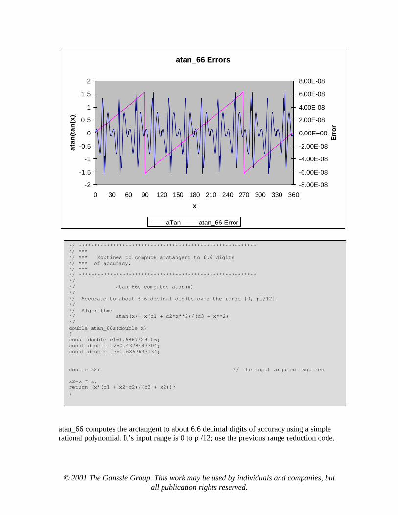
atan_66 computes the arctangent to about 6.6 decimal digits of accuracy using a simple rational polynomial. It’s input range is 0 to p /12; use the previous range reduction code.

// ********************************************************* // *** // *** Routines to compute arctangent to 6.6 digits // *** of accuracy. // *** // ********************************************************* // // atan_66s computes atan(x) // // Accurate to about 6.6 decimal digits over the range [0, pi/12]. // // Algorithm: // atan(x)= x(c1 + c2*x**2)/(c3 + x**2) // double atan_66s(double x) { const double c1=1.6867629106; const double c2=0.4378497304; const double c3=1.6867633134; double x2; // The input argument squared x2=x * x; return (x*(c1 + x2*c2)/(c3 + x2)); }

Better Firmware… Faster!

A One-Day Seminar

Presented at

Your Company

Does your

schedule prevent you from traveling?

This doesn’t mean you have to pass this great

opportunity by.

Presented by Jack Ganssle, technical editor of Embedded

Systems Programming Magazine, author of The

Art of Developing Embedded Systems, The

Art of Programming Embedded Systems, and The Embedded Systems

Dictionary

More information at www.ganssle.com

The Ganssle Group PO Box 38346

Baltimore, MD 21231 (410) 496-3647

fax: (647) 439-1454 [email protected] www.ganssle.com

For Engineers and Programmers This seminar will teach you new ways to build higher quality products in half the time. 80% of all embedded systems are delivered late… Sure, you can put in more hours. Be a hero. But working harder is not a sustainable way to meet schedules. We’ll show you how to plug productivity leaks. How to manage creeping featurism. And ways to balance the conflicting forces of schedules, quality and functionality. … yet it’s not hard to double development productivity Firmware is the most expensive thing in the universe, yet we do little to control its costs. Most teams deliver late, take the heat for missing the deadline, and start the next project having learned nothing from the last. Strangely, experience is not correlated with fast. But knowledge is, and we’ll give you the information you need to build code more efficiently, gleaned from hundreds of embedded projects around the world. Bugs are the #1 cause of late projects… New code generally has 50 to 100 bugs per thousand lines. Traditional debugging is the slowest way to find bugs. We’ll teach you better techniques proven to be up to 20 times more efficient. And show simple tools that find the nightmarish real-time problems unique to embedded systems. … and poor design creates the bugs that slip through testing Testing is critical, but it’s a poor substitute for well-designed code. Deming taught us that you cannot create quality via testing. We’ll show you how to create great designs that intrinsically yield better code in less time. Learn From The Industry’s Guru Spend a day with Jack Ganssle, well-known author of the most popular books on embedded systems, technical editor and columnist for Embedded Systems Programming, and designer of over 100 embedded products. You’ll learn new ways to produce projects fast without sacrificing quality. This seminar is the only non-vendor training event that shows you practical solutions that you can implement immediately. We’ll cover technical issues – like how to write embedded drivers and isolate performance problems – as well as practical process ideas, including how to manage your people and projects.

Seminar Leader

Jack Ganssle has written over 300 articles in Embedded Systems Programming, EDN, and other magazines. His three books, The Art of Programming Embedded Systems, The Art of Developing Embedded Systems, and his most recent, The Embedded Systems Dictionary are the industry’s standard reference works

Jack lectures internationally at conferences and to businesses, and was this year’s keynote speaker at the Embedded Systems Conference. He founded three companies, including one of the largest embedded tool providers. His extensive product development experience forged his unique approach to building better firmware faster. Jack has helped over 600 companies and thousands of developers improve their firmware and consistently deliver better products on-time and on-budget.

Course Outline Languages

• C, C++ or Java? • Code reuse – a myth? How can you benefit? • Stacks and heaps – deadly resources you can control.

Structuring Embedded Systems

• Manage features… or miss the schedule! • Do commercial RTOSes make sense? • Five design schemes for faster development.

Overcoming Deadline Madness

• Negotiate realistic deadlines… or deliver late. • Scheduling – the science versus the art. • Overcoming the biggest productivity busters.

Stamp Out Bugs!

• Unhappy truths of ICEs, BDMs, and debuggers. • Managing bugs to get good code fast. • Quick code inspections that keep the schedule on-track. • Cool ways to find hardware/software glitches.

Managing Real-Time Code

• Design predictable real-time code. • Preventing system performance debacles. • Troubleshooting and eliminating erratic crashes. • Build better interrupt handlers.

Interfacing to Hardware

• Understanding high-speed signal problems. • Building peripheral drivers faster. • Cheap – and expensive – ways to probe SMT parts.

How to Learn from Failures… and Successes

• Embedded disasters, and what we can learn . • Using postmortems to accelerate the product delivery. • Seven step plan to firmware success.

Do those C/C++ runtime routines execute in a usec or a week? This trig function is all over the map, from 6 to 15 msec. You’ll learn to rewrite real-time code proactively, anticipation timing issues before debugging.

Why Take This Course? Frustrated with schedule slippages? Bugs driving you batty? Product quality sub-par? Can you afford not to take this class? We’ll teach you how to get your products to market faster with fewer defects. Our recommendations are practical, useful today, and tightly focused on embedded system development. Don’t expect to hear another clever but ultimately discarded software methodology. You’ll also take home a 150-page handbook with algorithms, ideas and solutions to common embedded problems.

0

10

20

30

40

50

60

4950

5718

6486

7254

8022

8790

9558

10326

11094

11862

1263

0133

98141

66149

34

Microseconds

Pro

bab

ility

Here is what some of our attendees

have said:

If you can’t take the time to travel, we can present this seminar at your facility. We will train all of your developers and focus on the challenges

unique to your products and team.

Thanks for the terrific seminar here at ALSTROM yesterday!

It got rave reviews from a pretty tough crowd. Cheryl Saks, ALSTROM

Thanks for a valuable, pragmatic, and informative lesson in embedded systems design.

All the attendees thought it was well worth their time. Craig DeFilippo, Pitney Bowes

I just wanted to thank you again for the great class last week. With no exceptions, all of the feedback from the

participants was extremely positive. We look forward to incorporating many of the suggestions and observations into making our work here more efficient and higher quality.

Carol Bateman, INDesign LLC

Here are just a few of the companies where Jack has presented this seminar: Sony-Ericsson, Northup Grumman, Dell, Western Digital, Bayer, Seagate, Whirlpool, Cutler Hammer, Symbol, Visteon, Honeywell, Kodak and Western Digital.

Did you know that… … doubling the size of the code results in much more than twice the work? In this seminar you’ll learn ways unique

to embedded systems to partition your firmware to keep schedules from skyrocketing out of control. … you can reduce bugs by an order of magnitude before starting debugging? Most firmware starts off with a 5-

10% error rate – 500 or more bugs in a little 10k LOC program. Imagine the impact finding all those has on the schedule! Learn simple solutions that don’t require revolutionizing the engineering department.

… you can create a predictable real-time design? This class will show you how to measure the system’s performance,

manage reentrancy, and implement ISRs with the least amount of pain. You’ll even study real timing data for common C constructs on various CPUs.

… a 20% reduction in processor loading slashes development time? Learn to keep loading low while simplifying

overall system design. … reuse is usually a waste of time? Most companies fail miserably at it. Though promoted as the solution to the

software crisis, real reuse is much tougher than advertised. You’ll learn the ingredients of successful reuse. What are you doing to upgrade your skills? What are you doing to help your engineers succeed? Do you

consistently produce quality firmware on schedule? If not . . . what are you doing about it?

Contact us for info on how we can bring this seminar to your company. e-mail: [email protected] or call us at 410-496-3647.

a guide to approximationsnnp.ucsd.edu/phy120b/student_dirs/shared/gnarly/misc_docs/trig... · this...

Documents