a guide for atomic force microscopy analysis of soft- … · · 2007-12-19a guide for atomic...

A Guide for Atomic Force Microscopy Analysis of Soft-Condensed Matter

M. Raposo*, Q. Ferreira and P.A. Ribeiro 1CEFITEC, Departamento de Física, Faculdade de Ciências e Tecnologia, Universidade Nova de Lisboa,

2829-516 Caparica, Portugal In this chapter one intends to give practical insights for the characterization of soft condensed matter surfaces via atomic force microscopy (AFM). The most common causes of image artifacts are reviewed, solutions to avoid them proposed and good practices suggested. Quantities used to evaluate surface topographic features and its dynamics as result image processing data are also described.

Keywords AFM; artifacts; amplitude parameters; spacing parameters; hybrid parameters, statistical parameters; scale parameters

1. General remarks

The development of soft condensed matter surfaces at the molecular level is nowadays believed to be the building blocks for the creation of the next generation of materials and devices in practically all scientific areas. Particularly the buildup of functional macromolecular heterostructures and mimic of biological structures are in fact an actual trend. The advances in soft condensed analysis matter surfaces are mostly related with the atomic force microscopy (AFM) which was introduced in 1986 [1] and originated with the invention of the scanning tunneling microscope in 1982 by Binning and Rohrer [2,3]. These efemerids greatly enhanced the development of surface science and opened the field of nanoscience and nanotechnology as they allow to access to the molecular and atomic features. Nowadays several apparatus have been implemented and extensively used for surface analysis and manipulation at the atomic level, operating at different interface media, in several modes, such as contact non-contact tapping, allowing go further in the discovery of surfaces features occurring at the nanoscale level. Due to the tunneling effect, either electrical or optical in nature, being itself the base mechanism for detecting surface details, probed via a cantilever-tip or tuning fork mechanical systems, together with scanning features, attention has to be paid in what concerns to both handling and data processing in looking for consistency in results. In fact, the knowledge of the approaches in both measurement and data analysis when using AFM technique are essential for the correct interpretation of surface topographic features. Concerning to handling details, one of the most important factors come from the tip. In fact, both tip geometry and composition are known to influence the image quality. The major effects with regards to tip geometry are those leading surface feature broadening as a result of tip curvature’s radius being smaller or larger than the size of features. The tip to surface interaction local forces, for a given scanned area, may also affect the image as they are changing the tip compression conditions, which could cause the tip to move far from the optimum working distance for feature observation. This effect might lead the tip to move far away from the surface or too much close to it or even to hit it. Surface and tip contamination may also influence the measurement, namely if the size of the contaminant is close to that of the surface features. Other mechanical factors as those related with the cantilever’s calibration can also affect the results, mainly in what concerns to the determination of the appropriated elastic constant for a given cantilever-tip system. This could be relevant when force modulation mode is used as in measurement of force-distance curves which are relevant for studying surface molecular interactions and bond strength. Finally, there are other experimental factors that influence the accuracy in the attainment of the correct image, and are worth to refer, these are: image resolution, electric noise due to the tip- * Corresponding author: e-mail: [email protected], Phone: +351 21294 8576

©FORMATEX 2007Modern Research and Educational Topics in Microscopy. A. Méndez-Vilas and J. Díaz (Eds.)

758

_______________________________________________________________________________________________

induced electric field fluctuation and image data processing. All of these experimental aspects determine the data quality and could give rise to artifacts in the analysis of surface texture parameters such as roughness, grain size and surface fractal dimension. Concerning to data treatment as a result of a measurement, the choice of a data analysis method is always a complex issue requiring a quantitative statistical data analysis together with factors that are influencing it. Essentially this analysis is carried out at a single profile region and/or extended to the surface. In the first stage it is important to obtain the roughness parameters based on quantities as root mean square roughness, average height and grain diameter. In the case of kinetics studies, the overall surface roughness values can be obtained and roughness growth exponents determined allowing infer about the surface growth behavior. In addition, correlations between measurements, taken at different surface points, are calculated for a complete description of surface morphology. These will involve the calculation of the Power Spectrum Density (PSD) function, which provides a more reliable topography description and allows the determination surface’s fractal dimension, Autocovariance Function (ACF), giving an indication of the probability distribution of the random quantity. In addition, the determination of distribution of heights, skewness and kurtosis moment are fundamental for describing surface asymmetry and flatness features. In this chapter one intends to address some of the above issues concerning good experimental practices and data analysis capabilities, particularly when applied to the characterization of soft condensed matter surfaces observed mainly by using the non-contact mode.

2. Artifacts in Atomic Force Microscopy

The atomic force microscopy (AFM) belongs to a family of techniques dedicated to nanoscale surface characterization based in the concepts developed by Binning and Roher [1-3] for the scanning tunneling microscope (STM). Basically the AFM consists in the attainment of topographic images making probe scans over a surface, in a surface plane, x-y, while the distance between the surface and the probe, is being controlled [4-7]. The obtained topography image corresponds to the measured height values, z(x,y), for a given area, A, defined by a window scan size L. Each height value is associated to a pair of surface coordinates,(x,y), and the image may is described by a matrix with N lines and M columns which corresponds to the surface (x,y) points being the matrix elements the height z(x,y). The validity and accuracy of surface proprieties achieved via AFM are greatly influenced by both the measuring features as tip, cantilever, scan feature, and image data analysis procedure. By its importance in the achievement of results these factors will be discussed below.

2.1 Tip Effects

During the topography acquisition with an atomic force microscope (AFM), the interaction between the tip and the surface is dependent on the distance between both. When the interatomic distance is large, the attractive force between the tip and the surface is weak. As the tip is approaching further the attraction increases until the atoms are so close together that the electron clouds start to repel each other electrostatically. This signifies that the interaction force goes to zero at a distance of about few angstroms. Generally the topographies are obtained maintaining the interactions magnitude constant during the tip scanning, in both direct contact (contact) and intermittent contact (tapping) modes. In the contact mode, the tip wearing comes as a result of abrasive and adhesive contact with the surface which can lead to both tip contamination and surface damage. During the measurement in non contact mode deformations can also occur contributing for elastic wear out. Therefore the interactions between tip and surfaces may cause image artifacts and even surface damage. Moreover, the tip type to be used for a determined measurement is an important issue towards a good result, namely because the tip shape and composition is conditioned by sample nature. With respect to shape, tip artifacts may occur if the surface features have the same or smaller size than the AFM tip. In these cases the tip will not be able to correctly draw the profile contours giving rise to the so called convolution effects. One of the well known convolution effect is the feature broadening. This occurs when the tip curvature radius is

Modern Research and Educational Topics in Microscopy. A. Méndez-Vilas and J. Díaz (Eds.) ©FORMATEX 2007

759

_______________________________________________________________________________________________

comparable or greater than the feature size. For example, the silicon probes have radii of curvature in the range 5 to 15 nm, with half cone angles of about 10-30º, when used in the observation of biological samples, where normally the feature sizes are smaller than those of the tip, topographic profiles tend to be apart from real. To overcome the limitation of silicon tips during the observation of biological features, carbon nanotube tips have been successfully used to solve convolution effects. The diameter of these tips is close to that of major small organic molecules and additionally offer good mechanical properties [8,9,10]. As a reference to minimize tip convolution, McEuen et al [11] used carbon nanotube technology (CNT) to image protein complex in a mica surface. The CNT tips, with 1 to 2 nm of diameter, were prepared via chemical vapor deposition and were mounted onto standard Pt/Ir coated AFM tips. This technology demonstrated that when tip structure has the same properties of the surface to be analyzed the results are very reproducible. In addition, other desirable properties of CNT tips for analyzing biological samples were revealed, these are low tip-sample adhesion, ability to resist large forces, possibility of achieving high lateral imaging resolution and capability of being chemically functionalized. In fact, DNA AFM images scanned with silicon tip, Pt/Ir coated tip and single-walled CNT tip were compared and the last one demonstrated notable resolution and reproducibility.

Fig. 1 Schematization of broadening effect in AFM image due to tip size effect, observable when tip size is comparable with the surface feature size. Tip contamination may also give rise to convolution which is related with the contaminant size relative to surface size features to be measured. Therefore, before each measurement the verification of the tip state has to be addressed. McIntyre et al [12] proposed a method to evaluate the tip status, using the scan of a biaxialy oriented polypropylene (BOPP) film for reference. If the tip is contaminated or even damaged the characteristic fiber-like network source will not be detected. In fact, BOPP is a good reference for testing tips because is soft, hydrophobic and has low surface energy, which are important factors preventing the tip contamination [13]. Another negative influence in the image is the tip compression on the feature to be observed. This happens when the tip is over the feature compressing it. This compression may give rise to surface damage and consequently causing an artifact in the obtained image. At this point it is worth to remark that carbon nanotube tips have demonstrated good flexibility, which limits the maximum force applied to the sample and prevents surface damage [14]. Computational calculations of the flexibility of CNT tips lead to values of maximum force of about 50 pN instead of the value of 100 nN found when using a standard AFM tip. Generally in looking for high-resolution in AFM imaging of a soft or fragile surface a sharp tip and a soft cantilever is recommended. Cantilever features will be discussed in the next section.

2.2 Cantilever System

The most common cantilevers used in AFM are the rectangular shape and V-shape, made of silicon or silicon nitride. The desirable conditions for a cantilever are low spring constant and high resonant frequencies. An AFM measurement free of artifacts requires the cantilever calibration, which consists on the elastic constant determination and in the deliberation if the stiffness is adequate to observe a given


760

_______________________________________________________________________________________________

surface. The normal cantilever spring constant, kz, is defined as the ratio of the applied normal force (Fz) at the cantilever tip position to the deflection in the normal direction at that position (∆z), which can be expressed by z z zk F= ∆ [15]. The determination of the cantilever elastic constant should be a standard procedure in all AFM measurements. As an example, in contact mode the cantilever elastic constant limits both the minimum tracking force exerted on the surface during scan and the speed scan [16]. The knowledge of the frontier values is important to prevent tip performance damage. In non-contact mode the value of cantilever elastic constant essentially limits the imaging scan speed. A review on the principal methods for achieving the so called cantilever elastic or spring constant calibration has been written by Burnham and Tendler [17]. In addition, recently Cumpson [18] presented a new method for AFM spring constant calibration based in a reference cantilever, where a precision of ± 3% can be achieved. Several examples of soft matter analysis demonstrated the relevance in accurate spring constants, calibration particularly when force curves measurements are intended [19,20].

2.3 Image Processing Features

Before analyzing AFM images it is necessary to optimize the image quality exploring the software facilities. Sometimes surface features are not visible before adequate image treatment and in other cases the image processing methods may hide important features. Often images reveal distortions caused by either tilt samples or non linear scanner behavior. Usually the first step is to remove artifacts due to leveling which basically consists in removing tilt sample image. This process is schematized in fig.2. The most common method for AFM image leveling is the so called line by line. It consists in fitting an image profile line with a polynomial equation which is then subtracted from that image line. After this the average height of each line is set equal to the previous corrected line. Care must be taken with this method, particularly when the image presents some isolated features on a very flat surface. In these cases line leveling may cause image artifact since the polynomial fitting may include the feature, causing streak marks in the image. In these cases it is necessary exclude the feature of the polynomial fitting, an example of that is shown in fig. 3.

Fig. 2 Schematization of the leveling process: a) Image profile showing tilt effect and b) Image after correction of tilt. Other commonly used method consists in taking three selected points and to subtract the plane formed by them from the image. This method is suitable when the sample presents a terrace where the background associated with the scanner is much lower than the terraces heights. Leveling is not always sufficient to attain an accurate image. In some cases it is necessary clean noise in the image using filters. Noise is often present in the AFM images and can be caused by irregularities in the surface roughness, sample impurities, humidity, to wear of AFM components, mechanical instabilities and electronic instabilities. Two types of filtering are commonly adressed in AFM images for noise elimination: the matrix filtering and Fourier. In the Matrix Filtering it is possible to choose between low, median or high filtering process. The filtering process is performed by replacing the center pixel in a square matrix, like 3x3, 5x5 or 7x7, with a low, median, or high z value, depending on the selected filter, of the pixels in the matrix. This matrix filtering process is to be extended to all image pixels. As a remark, this kind of filtering tends to erroneously delete the features end points. In Fourier filtering (FFT), the image frequency components are calculated to give rise to a set off FFT images. After this procedure, unwanted frequency components can be identified and removed from the FFT image. Kienberger et al [21] compared single cell image as a result of applying to the image three


761

_______________________________________________________________________________________________

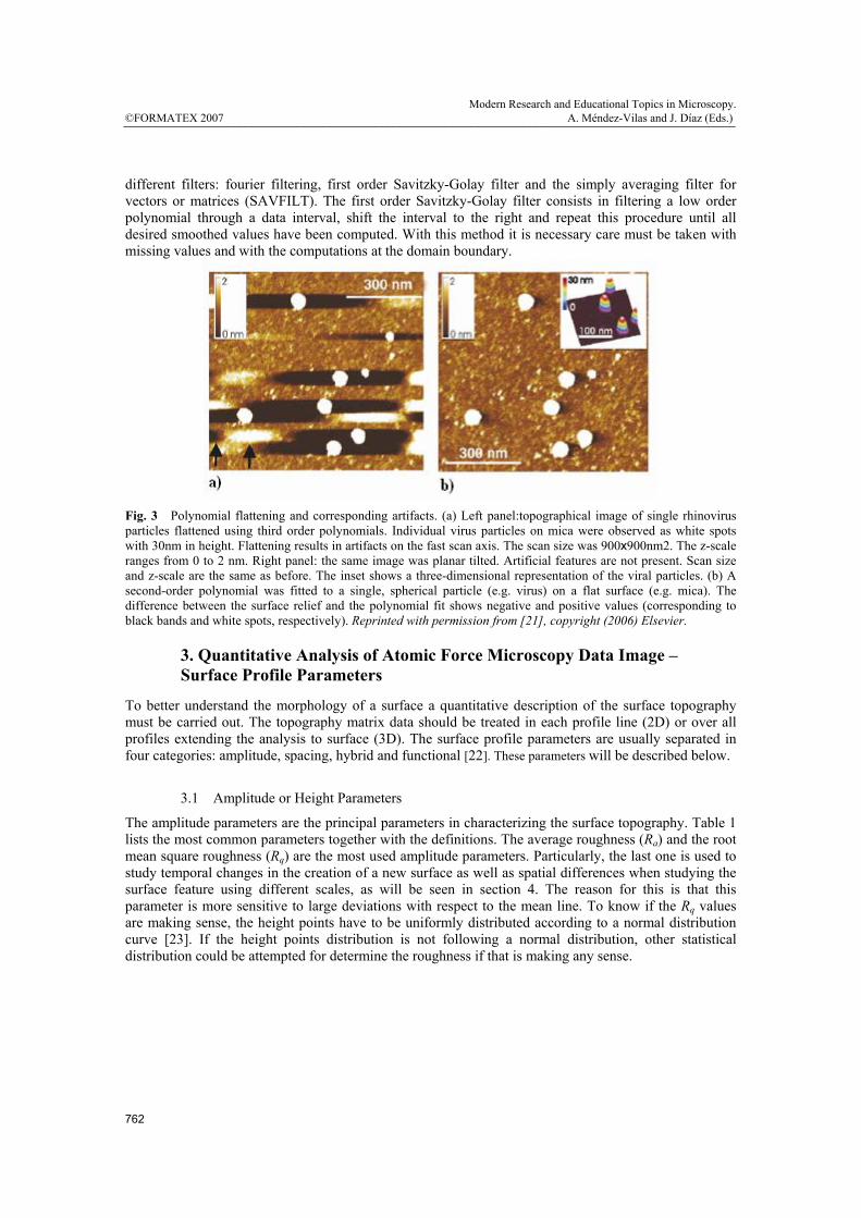
different filters: fourier filtering, first order Savitzky-Golay filter and the simply averaging filter for vectors or matrices (SAVFILT). The first order Savitzky-Golay filter consists in filtering a low order polynomial through a data interval, shift the interval to the right and repeat this procedure until all desired smoothed values have been computed. With this method it is necessary care must be taken with missing values and with the computations at the domain boundary.

Fig. 3 Polynomial flattening and corresponding artifacts. (a) Left panel:topographical image of single rhinovirus particles flattened using third order polynomials. Individual virus particles on mica were observed as white spots with 30nm in height. Flattening results in artifacts on the fast scan axis. The scan size was 900x900nm2. The z-scale ranges from 0 to 2 nm. Right panel: the same image was planar tilted. Artificial features are not present. Scan size and z-scale are the same as before. The inset shows a three-dimensional representation of the viral particles. (b) A second-order polynomial was fitted to a single, spherical particle (e.g. virus) on a flat surface (e.g. mica). The difference between the surface relief and the polynomial fit shows negative and positive values (corresponding to black bands and white spots, respectively). Reprinted with permission from [21], copyright (2006) Elsevier.

3. Quantitative Analysis of Atomic Force Microscopy Data Image – Surface Profile Parameters

To better understand the morphology of a surface a quantitative description of the surface topography must be carried out. The topography matrix data should be treated in each profile line (2D) or over all profiles extending the analysis to surface (3D). The surface profile parameters are usually separated in four categories: amplitude, spacing, hybrid and functional [22]. These parameters will be described below.

3.1 Amplitude or Height Parameters

The amplitude parameters are the principal parameters in characterizing the surface topography. Table 1 lists the most common parameters together with the definitions. The average roughness (Ra) and the root mean square roughness (Rq) are the most used amplitude parameters. Particularly, the last one is used to study temporal changes in the creation of a new surface as well as spatial differences when studying the surface feature using different scales, as will be seen in section 4. The reason for this is that this parameter is more sensitive to large deviations with respect to the mean line. To know if the Rq values are making sense, the height points have to be uniformly distributed according to a normal distribution curve [23]. If the height points distribution is not following a normal distribution, other statistical distribution could be attempted for determine the roughness if that is making any sense.


762

_______________________________________________________________________________________________

Table 1 Principal amplitude or height parameters.

Parameter Definition Arithmetic average height ( z )

General description of height variations.

( ) ( )1

1, ,N

x

z N M z x yN =

= ∑ (2D)

( ) ( )1 1

1, ,N M

x y

z N M z x yNM = =

= ∑∑ (3D)

Average roughness (Ra) Gives the deviation in height. Different profiles can give the same Ra.

( ) ( ) ( )( )1

1, , ,N

ax

R N M z x y z N MN =

= −∑ (2D)

( ) ( ) ( )( )1 1

1, , ,N M

ax y

R N M z x y z N MNM = =

= −∑∑ (3D)

Root Mean Square (RMS) roughness (Rq)

Represents the standard deviation of surface heights.

( ) ( ) ( )( )2

1

1, , ,N

qx

R N M z x y z N MN =

= −∑ (2D)

( ) ( ) ( )( )2

1 1

1, , ,N M

qx y

R N M z x y z N MNM = =

= −∑∑ (3D)

Total roughness (Rt) t p vR R R= +

Maximum profile peak height (Rp)

Height of the highest peak above the mean line in the profile. ( )max ;1p iR z z i N= − < <

Maximum profile valley depth (Rv)

Depth of the deepest valley below the mean line in the profile. ( )min ;1v iR z z i N= − < <

Average maximum profile peak heights(Rpm)

Mean of maxima profile peak height calculated over the surface.

1

1 M

pm pjj

R RM =

= ∑

Average maximum profile valley depths (Rvm)

Mean of maxima profile valleys depths calculated over the surface.

1

1 M

vm vjj

R RM =

= ∑

Average total roughness(Rt)

tm pm vmR R R= +

Ten Point Height (Rz(iso)) The difference in height between the average of the five highest peaks and the five lowest valleys along the assessment length of the profile.

( )5 5

1 1

1z pi vi

i i

R iso R Rn = =

= + ∑ ∑

If a given height profile in a surface presents deviations from both average roughness and RMS roughness, then the measurement should be repeated. A large number of peaks and valleys in an image significantly affect the Ra and Rq values and in these cases it is preferable to calculate the average peak-to-valley difference. Brogueira et al [24] used this peak-to-valley height parameter to measure a periodic structure of urethane/urea elastomeric film. The tapping mode was used to observe the periodic pattern on the polymer surface and the periodic peaks grouped in pairs for calculations.


763

_______________________________________________________________________________________________

Fig. 4 Top view of the topography of the free surface of urethane/urea film. The AA´ and BB´cross-sections were taken along the lines marked on the top of view image. AA´was taken along d2 and BB´ along d1. In AA´ height profile the two marks indicate the repeating spatial period characterized by a well-established complex structure of eight peaks and valleys. Reprinted with permission from[24] copyright (2003) Elsevier.

3.2 Spacing Parameters

The spacing parameters are based in the measurement of the horizontal or lateral features of the surface. The features that determine a spacing parameter are usually related with peaks and valleys regions. These parameters are useful for optimizing the surface quality in metal industry, in bending, forming tools and painting processes [25]. They are also important for controlling the porosity of membranes [26-29].

a) b)

Fig. 5 a) AFM topography with area window 2 x 2 µm2 of a PAH/PAZO bilayer and b) High Spot Count (HSC) and peak count for the marked profile in the topography, in this case the upper and lower thresholds corresponds to Ra value.


764

_______________________________________________________________________________________________

Table 2 List of spacing parameters.

Parameter Definition Peak count threshold Defined line distanced from the mean line ( z ) to a chosen value. It is

recommendable to choose as threshold the Ra value. One can define also the lower threshold and the upper threshold which are below and above the mean line. A peak must cross above the upper threshold and below the lower threshold or the mean line depending on the parameter to be calculated.

Peak Count or Peak Density (Pc) Number of peaks crossing above the upper threshold and below the lower threshold per length of trace in a profile, i.e, the number of peaks observed in the evaluation length divided by the evaluation length.

High spot count (HSC) Number of high peaks above one select band per unit length along the assessment length. This definition is similar to peak count except that a peak is defined relative to only one threshold.

1

n

aa

HSC P=

= ∑

Mean spacing of adjacent local peaks (S)

Average spacing of adjacent local peaks in the profile. The local peak is the highest part of the profile considered between two adjacent minima and is only measured if the vertical distance between the adjacent peaks is greater than or equal to 10% of the maximum height of the profile.

1

1 n

ii

S Sn =

= ∑

n – number of local peaks along the profile.

Mean Spacing at Mean line (Sm) Average spacing of adjacent local peaks in the profile being n is number of profile peaks along the profile. The profile peak is the highest point of the profile between upwards and downwards crossing the mean line.

m1

1S =N =

∑n

ii

S

Number of intersections of the profile at the mean line (n(0))

Number of intersections in the profile (ci), being L the profile length.

1

1n(0)=L =

∑n

ii

c

Number of peaks in the profile (m) Number of peaks of the profile per unit length.

1

1m=L =

∑n

ii

m

Number of inflection points (g) Number of inflection points in the profile per unit length:

1

1g=L =

∑n

ii

g

3.2 Hybrid Parameters

Hybrid parameters are a combination of amplitude and spacing features of surface, useful for studying mechanical and tribological properties of surfaces such as friction, elastic contact, reflectance, fatigue crack initiation and hydrodynamic lubrication. The fundamental hybrid parameters are listed and described in table 3.


765

_______________________________________________________________________________________________

Table 3 List and description of hybrid parameters.

Parameter Definition Profile slope at mean line (γ) Profile slope at the mean line is obtained for calculating the average of the

individual profile slopes at each intersection with the mean line. 1

1

1

1 tan1

ni

i i

zn x

γ−

−

=

∂= − ∂

∑

Being n the total number of intersections of the profile with the mean line along the assessment length.

Average absolute slope or mean slope of the profile(∆a)

Mean absolute profile slope over the assessment length, obtained calculating the average of all slopes between each two successive points of the profile:

1

1

11

Ni

i i

zaN x

−

=

∂∆ =

− ∂∑

Root mean square (RMS) slope of the profile(∆q)

Root mean square of the mean profile slope. 2

1 11

1 1 1

1 11 1

N Ni i i

qi ii i i

z z zN x N x x

− −−

= = −

∂ −∆ = − − ∂ − −

∑ ∑

Average wavelength (λa) Spacing between local peaks and valleys, considering their relative amplitudes and individual spatial frequencies.

2 aa

a

Rπλ =∆

Root mean square wavelength (λq) Root mean square of the spacing between local peaks and valleys, considering their relative amplitudes and individual spatial frequencies.

2 qq

q

Rπλ =

∆

Relative length of the profile (lo) Sum of the lengths of the profile individual parts divided by the assessment length.

( )21

1

1 ;n

o i i i i ii

l l l z z xL

δ+=

= = − +∑

Stepness factor of the profile (Sf) Ratio between the arithmetic average height (Ra) and the mean spacing of the profile (Sm).

af

m

RSS

=

Waviness factor of the profile (Wf) Ratio between the total range of the entire profile and the arithmetic average height (Ra) being n is the number of points along the profile.

1

1

1 n

f iia

W lR

−

=

= ∑

3.4 Functional or Statistical Parameters and Functions

The functional or statistical parameters and functions, listed and described in table 4, give information about the surface structure. For example the power spectral density function may provide quantitative information about roughness, growth regime, grains size and correlation length [30,31]. The distribution functions as amplitude distribution function are other examples allowing calculation Skewness (RSk) and Kurtosis (RKu) moments which are parameters used to measure the asymmetry and the flatness, respectively.


766

_______________________________________________________________________________________________

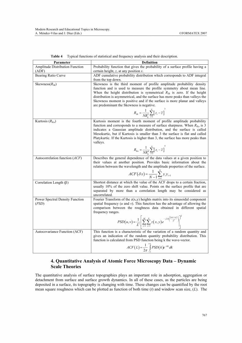
Table 4 Typical functions of statistical and frequency analysis and their description.

Parameter Definition Amplitude Distribution Function (ADF)

Probability function that gives the probability of a surface profile having a certain height, z, at any position x.

Bearing Ratio Curve ADF cumulative probability distribution which corresponds to ADF integral from the top down.

Skewness(RSk) Skewness is the third moment of profile amplitude probability density function and is used to measure the profile symmetry about mean line. When the height distribution is symmetrical RSk is zero. If the height distribution is asymmetrical, and the surface has more peaks than valleys the Skewness moment is positive and if the surface is more planar and valleys are predominant the Skewness is negative.

[ ]3

31

1 N

Sk iiq

R z zNR =

= −∑

Kurtosis (RKu) Kurtosis moment is the fourth moment of profile amplitude probability function and corresponds to a measure of surface sharpness. When RKu is 3 indicates a Gaussian amplitude distribution, and the surface is called Mesokurtic, but if Kurtosis is smaller than 3 the surface is flat and called Platykurtic. If the Kurtosis is higher than 3, the surface has more peaks than valleys.

[ ]4

41

1 N

Ku iiq

R z zNR =

= −∑

Autocorrelation function (ACF) Describes the general dependence of the data values at a given position to their values at another position. Provides basic information about the relation between the wavelength and the amplitude properties of the surface.

( ) 11

11

N

i ii

ACF x y yN

δ +=

=− ∑

Correlation Length (β) Shortest distance at which the value of the ACF drops to a certain fraction, usually 10% of the zero shift value. Points on the surface profile that are separated by more than a correlation length may be considered as uncorrelated.

Power Spectral Density Function (PSD)

Fourier Transform of the z(x,y) heights matrix into its sinusoidal component spatial frequency (u and v). This function has the advantage of allowing the comparison between the roughness data obtained in different spatial frequency ranges.

( ) ( )( )

2

22

21 1

1, ,ux vyM N j

L

y x

PSD u v z x y eL

π+

−

= =

= ∑∑

Autocovariance Function (ACF) This function is a characteristic of the variation of a random quantity and gives an indication of the random quantity probability distribution. This function is calculated from PSD function being k the wave-vector.

( ) ( )12

ikLACF L PSD k e dkπ

+∞−

−∞

= ∫

4. Quantitative Analysis of Atomic Force Microscopy Data – Dynamic Scale Theories

The quantitative analysis of surface topographies plays an important role in adsorption, aggregation or detachment from surface and surface growth dynamics. In all of these cases, as the particles are being deposited in a surface, its topography is changing with time. These changes can be quantified by the root mean square roughness which can be plotted as function of both time (t) and window scan size, (L). The


767

_______________________________________________________________________________________________

surface buildup can be now be interpreted, using that data in dynamic scale theory and fractal concepts [7]. In fact, from the roughness as a function of time and scanning window size or scale one can determine parameters such as roughness and growth critical exponents and fractal dimension [32,33,34]. Definitions for these parameters are displayed and described in table 5.

Table 5 Scale parameters.

Parameter Definition Growth exponent (β) Characterizes the time dependence of the roughness. The roughness values

for the different times must be taken for a constant LxL window.

( ),qR L t t β∝

Roughness critical exponent (α) The determination of α requires that the film roughness to be taken after the roughness saturation regime has been attained, i.e, when the roughness is time independent.

( ),qR L t Lα∝

Fractal Dimension (DF) DF = D-α

The roughness exponents are often used to understand the behavior of some organic thin films, namely in what concerns to buildup of surfaces and in several cases it is also possible to determine the β exponent considering the film thickness [35,7]. Relevance of these parameters is exemplified in the work of de Souza et al [36] which used the roughness exponent (α) to determine the influence drying procedures in poly (o-methoxyaniline) (POMA) alternated with poly (vinyl sulfonic acid) (PVS) layer-by-layer (LBL) polyelectrolyte films where the changes in LBL films buildup where investigated using AFM and roughness exponents were obtained. The fractal dimension was calculated for POMA/PVS films adsorbed onto several substrates, was found to decrease with the number of bilayers. For films prepared onto silicon the fractal dimension varied from 2.9 for one bilayer to 2.58 for 14 bilayers. These values indicate that the roughness of the surface is decreasing with the number of bilayers.

5. Final remarks

This chapter addresses the principal features of atomic force microscopy in both surface morphology and surface growth characterization. Emphasis was given to artifact, handling, data analysis and quantification of surface morphology.

Acknowledgements The support by from FCT/MCES-POCTI/FAT/47529/2002 (Portugal) is gratefully acknowledged.

References

[1] G. Binning, C. Quate and Ch. Gerber, Phys. Rev. Lett. 56, 930, 1986 [2] G. Binnig, H. Rohrer, CH. Gerber and E. Weibel, Phys. Rev. Lett. 49, 57, 1982 [3] G. Binnig and H. Rohrer, Reviews of Modern Physics 71, S324, 1999 [4 ] G. Binnig and D.P.E. Smith, Rev. Sci. Instrum. 57, 1688 (1986) [5] M.G.L. Gustafsson and J. Clarke, J. Appl. Phys. 76, 172, 1994 [6] S.N. Magonov and M-H. Whangbo, Surface analysis with STM and AFM, (VCH, Weinheim 1996) [7] M. Raposo, P.A. Ribeiro, M.A. Pereira da Silva, O.N. Oliveira Jr., in Current Issues on Multidisciplinary Microscopy Research and Education, edited by A. Méndez-Vilas and L.Labajos-Broncano, FORMATEX Microscopy Book Series N.2, pp. 224-241, 2004 [8] L. Chen, C. L. Cheung, P. D. Ashby, C. M. Lieber, Nanno Letters, 4, 1725, 2004NO


768

_______________________________________________________________________________________________

[9] R.M.D. Stevens, N. A Frederick, B. L Smith, Nanotechnology 11, 1, 2000 [10] Y. Wanga, X. Chen, Ultramicroscopy 107, 293, 2007 [11] J S Bunch, TN Rhodin and P L McEuen, Nanotechnology 15, S76, 2004 [12] H. Y. Nie and N.S McIntyre, Langmuir 17, 432, 2001 [13] H.-Y. Nie, M. J. Walzak, and N. S. McIntyre, Review of Scientific Instruments, 73, 3831, 2002 [14] L. Guo, R. Wang, H. Xu, Ji Liang, Physica E 27, 240, 2005 [15] J. E. Sader, Review od Science Instruments, 74, 2438, 2003 [16] J.P. Cleveland and S. Manne, Rev. Sci. Instrum. 64, 403, 1993 [17] N. A. Burnham, X Chen, C. S. Hodges, G. A. Matei, E.J.Thoreson, C. J.Roberts, M. C. Davies and S. J. B.

Tendler, Nanotechnology 14, 1, 2003 [18] P. J. Cumpson, C. A Clifford and J. Hedley, Meas. Sci. Technol 15, 1337, 2004 [19] S. B. Velegol and B. E. Logan, Langmuir 18, 5256, 2002 [20] M. A. Plunkett, A. Feiler and M. W. Rutland, Langmuir 19, 4180, 2003 [21] F. Kienbergera, V.P. Pastushenkoa, G. Kadab, T. Puntheeranuraka, L. Chtcheglovaa, C. Riethmuellerc, C. Rankla, A. Ebnera, P. Hinterdorfer, Ultramicroscopy 106, 822, 2006 [22] E.S. Gadelmawla, M.M. Koura, T.M.A. Maksoud, M. Elewa, H.H. Soliman, Journal of Materials Processing

Technology 123, 133, 2002 [23] A.Maksumov, R.Vidu, A.Palazoglu and P.Stroeve, , Journal of Colloid and Interface Science 272, 365, 2004 [24] M. H. Godinho, L.V. Melo and P. Brogueira, Materials Science & Engineering C, 23, 919, 2003. [25] K. G.Gunde, M.Kunaver and M. Čekada, Dyes and Pigments, 74, 202, 2007 [26] J.A. Otero, G. Lena , J.M. Colina, P. Prádanos , F. Tejerina , A. Hernández, Journal of Membrane Science 279,

410, 2006 [27] T.-Y. Liu , Wen-Ching Lin , M.-C. Yang , S.-Y. Chen, Polymer 46, 12586, 2005 [28] N. Hilal , H. AI-Zoubi , N.A. Darwish and A.W. Mohammad, Desalination 177, 187, 2005 [29] M. Khayet , K.C. Khulbe , T. Matsuura, Journal of Membrane Science 238, 199, 2004 [30] P. Brault, P.Dumas, F.Salvan: J. Phys.: Condens. Matter 10, L27, 1998

[31] E. A. Eklund, E. J. Snyder, R. S. Williams, Surface Science, 285, 157, 1993

[32] R.F.M. Lobo, M.A. Pereira-da-Silva, M. Raposo, R.M. Faria and O.N. Oliveira Jr, Nanotechnology, 14, 101, 2003

[33] N.C. de Souza, J.R. Silva, R. Di Thommazo, M. Raposo, D.T. Balogh, J. A. Giacometti and O. N. Oliveira Jr., J. Phys. Chem. B 108, 13599, 2004.

[34] F.L. Leite, L.G. Paterno, C.E. Borato, P.S.P. Herrmann, O.N.Oliveira Jr, L.H.C.Mattoso, Polymer 46, 12503, 2005

[35] A.E.Lita, J.E.Sanchez, Jr., J. Appl. Phys. 85, 876, 1999 [36] N. C. de Souza, J. R. Silva, M. A. Pereira-da-Silva, M. Raposo, R. M. Faria, J. A. Giacometti and O. N. Oliveira

Jr., Journal of Nanoscience and Nanotechnology 4, 548, 2004


769

_______________________________________________________________________________________________

a guide for atomic force microscopy analysis of soft- … · · 2007-12-19a guide for atomic...

Documents