a grass-datamining integrated procedure for land cover

A GRASS-DataMining integrated procedure for land cover classification

ALFONSO VITTI, MARCO BEZZI

Department of Civil and Environmental Engineering University of Trento, Italy

via Mesiano 77, 38100 Trento [email protected] [email protected]

Abstract

Combining some of the features provided by the GRASS GIS and Data Mining algorithms, an integrated procedure has been developed to produce a supervised land cover classification at 30 m spatial resolution using Landsat TM images and the DTM (Digital Terrain Model) of an area in the Adige Valley (Trento, Italy). While the classification of satellite images is often in general mainly based on the radiometric information, in this work some morphological information have been used to integrate the parameters that the classification model learns by. Both radiometric and morphologic information have been extracted and managed using GRASS to define the input data-set for the KDD (Knowledge Discovery in Databases) algorithms. Various well known Machine Learning (ML) algorithms have been applied to understand their main features, usability and accuracy. The ML algorithm of the model performing the best classification has therefore been applied to the entire study area using the GRASS raster map-algebra capabilities to produce the classified map. The derived model is based on the C4.5 decision tree algorithm and presents a quite simple structure and an accuracy of 93% on the test set. Visual comparison of the final map with the orthorectifieded RGB aerial image of the studied area also reveals a good general agreement.

1.Introduction Aim of this work is to understand how a KDD (Knowledge Discovery in Databases) approach can be followed to produce land cover classification model. Since many ML (Machine Learning) algorithms are available various test have been performed to allow the understanding the difference between different methods in term of accuracy and consistency with domain knowledge. Data Mining (DM) is often use to perform land cover classification using satellite images and known information on the land cover on some small areas. In this work some ground morphological information have been integrated with remotely sensed data to better describe the land surface and better predict land coverage. The task is to produce a method to predict land cover using both multi-spectral satellite images and morphological information of the studied region. The Weka software [http://www.cs.waikato.ac.nz/~ml/] has been used to apply the ML algorithms used in this study. Weka is a collection of machine learning algorithms for data mining tasks. Weka contains tools for data pre-processing, classification, regression, clustering, association rules, and visualization. It is written entirely in Java and it is open source software issued under the GNU General Public License. The GRASS GIS has been used to manage and to extract the geographical information: the Landsat TM images and the DTM have been managed as raster files. From the DTM the information of the ground slope and aspect values have been extracted through the r.slope.aspect module and used, along with the terrain height, to integrate the radiometric information. For each ML algorithm, Weka produces a classification method and supplies some statistical information on its accuracy. The classifier performing the best results has been implemented within the GRASS GIS to produce the land cover map of the study region. 2.Domain description The studied area is 5 km x 5 km and it is located in the Trentino Alto Adige region (Italy), 15 km north of Trento

mailto:[email protected]

mailto:[email protected]

http://www.cs.waikato.ac.nz/~ml/

where the Val di Sole meets the Adige Valley (Fig. 9). The orogenesis of the two valleys is glacial and both have typical U cross section, the lowland of the two valley is quite large and it is mostly covered by vineyards and urban zone, while the mountains have very steep slopes with plateaus on the top. The area could be divided into five major types of land cover, namely: civil constructions, conifer forest, broad-leaved forest, vineyards and rock slopes. Civil constructions and vineyards are mostly situated low land while forests and rock slopes are located in higher areas. The zone has been chosen for the morphologic variability, the obvious land cover characterization and the availability of Landsat TM image, DTM and orthorectify RGB an aerial photogrammetric image. 3.Data description The data used in this work are:

Landsat 7 TM image; Digital Terrain Model at 10 m x 10 m spatial resolution; Orthorectifieded RGB aerial photogrammetric image at 1 m x 1 m spatial resolution.

The data for a single scene taken by the Landsat 7 includes the ETM+ sensor 7 bands information and the panchromatic sensor information, which are stored as image data. The images are usually corrected for radiometric and geometric distortions and are then made available as a complete set of raw data.

Band Spectral Range [microns] Electromagnetic Spectrum Resolution[m]

1 0.450 to 0.515 Visible blue-green 30

2 0.525 to 0.605 Visible green 30

3 0.630 to 0.690 Visible red 30

4 0.750 to 0.900 Near infrared 30

5 1.550 to 1.750 Mid-infrared 60

6 10.400 to 12.500 Thermal infrared 30

7 2.090 to 2.350 Mid-infrared 30

Pan 0.520 to 0.900 Visible light 15

Tab. 1 Landsat 7 TM multi-spectral bands.

The Provincia Autonoma di Trento, the local government agency, has provided the Digital Terrain Model and the ortho-photo. Since the dataset presents different spatial resolutions, a 30 m x 30 m resolution has been chosen to allow a consistency use of the land information. All the dataset has been imported in GRASS and the resolution of the DTM and of the ortho-photo have been reduced to reach the Landsat 30 m x 30 m resolution. The land cover classification derived from remotely sensed data can basically performed using the bands 2 (green), 3 (red), 4 (near-infrared) and the Normalized Difference Vegetation Index (NDVI). The NDVI is obtained combining the bands 3 and 4 as: NDVI = (band 4 - band 3) / (band4 + band 3) No other Landsat bands have been considered in the study. The choice of using a small number of bands has allowed a simpler and quicker analysis of the influence of the bands on the results of the ML algorithms. The analysis of such influence has been, in this study, more relevant than produce a complex and precise model. To allow Weka to manage the morphological information the slope and aspect values, originally continuous numerical values, have been re-classified in discrete interval as follows:

Class 1 (north)

2 (north-east)

3 (east)

4 (south-east)

5 (south)

6 (south-west)

7 ( west)

8 (north-west)

Values [°] -22.5 22.5

22.5 67.5

67.5 112.5

112.5 157.5

157.5 202.5

202.5 247.5

247.5 292.5

292.5 337.5

Tab. 2 Aspect values re-classification.

Class 1 2 3 4 5 6 7 8 9 10 11

Values [°] 0 – 5 5 – 10 10 – 15 15 – 20 20 – 30 30 – 40 40 – 50 50 – 60 60 – 70 70 – 80 80 - 90

Tab. 3 Slope values re-classification.

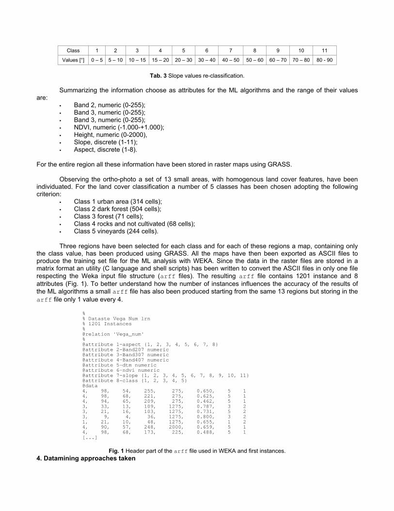
Summarizing the information choose as attributes for the ML algorithms and the range of their values are:

Band 2, numeric (0-255); Band 3, numeric (0-255); Band 3, numeric (0-255); NDVI, numeric (-1.000-+1.000); Height, numeric (0-2000), Slope, discrete (1-11); Aspect, discrete (1-8).

For the entire region all these information have been stored in raster maps using GRASS. Observing the ortho-photo a set of 13 small areas, with homogenous land cover features, have been individuated. For the land cover classification a number of 5 classes has been chosen adopting the following criterion:

Class 1 urban area (314 cells); Class 2 dark forest (504 cells); Class 3 forest (71 cells); Class 4 rocks and not cultivated (68 cells); Class 5 vineyards (244 cells).

Three regions have been selected for each class and for each of these regions a map, containing only

the class value, has been produced using GRASS. All the maps have then been exported as ASCII files to produce the training set file for the ML analysis with WEKA. Since the data in the raster files are stored in a matrix format an utility (C language and shell scripts) has been written to convert the ASCII files in only one file respecting the Weka input file structure (arff files). The resulting arff file contains 1201 instance and 8 attributes (Fig. 1). To better understand how the number of instances influences the accuracy of the results of the ML algorithms a small arff file has also been produced starting from the same 13 regions but storing in the arff file only 1 value every 4.

% % Dataste Vega Num lrn % 1201 Instances % @relation 'Vega_num' % @attribute 1-aspect {1, 2, 3, 4, 5, 6, 7, 8} @attribute 2-Band207 numeric @attribute 3-Band307 numeric @attribute 4-Band407 numeric @attribute 5-dtm numeric @attribute 6-ndvi numeric @attribute 7-slope {1, 2, 3, 4, 5, 6, 7, 8, 9, 10, 11} @attribute 8-class {1, 2, 3, 4, 5} @data 4, 98, 54, 255, 275, 0.650, 5 1 4, 98, 68, 221, 275, 0.625, 5 1 4, 94, 65, 209, 275, 0.462, 5 1 3, 33, 13, 109, 1275, 0.787, 3 2 3, 21, 16, 103, 1275, 0.731, 5 2 3, 9, 4, 36, 1275, 0.800, 3 2 1, 21, 10, 48, 1275, 0.655, 1 2 4, 90, 57, 248, 2000, 0.659, 5 1 4, 98, 68, 173, 225, 0.488, 5 1

[...]

Fig. 1 Header part of the arff file used in WEKA and first instances.

4. Datamining approaches taken

Different ML algorithms, implemented in the WEKA software, have been used and tested with different parameters and options. Figure 2 reports a logical schema of the procedure that has to be followed to allow the ML algorithms to “learn” the classification model from the classified dataset, i.e. the 13 homogenous areas selected from the ortho-photo. The apriori-classified regions have to be spitted in two sub-sets: the training and the test set. The training-set is used, by the ML algorithms, to derive the classification model while the test-set is used to verify the capability, i.e. the accuracy, of the derived model. In this way the model is tested over a pre-classified dataset that has not be used in the learning procedure, statistical analyses are performed to estimate the agreement between predicted and “true” values. The definition of the training and of the test set can be carried out through different techniques: percentage splitting, random splitting, user-defined splitting, cross-validation. The ML algorithms tested are/have been:

Decision Rules; J48 (C4.5); Naïve Bayes; IB1 (nearest neighbor); BK (k-nearest neighbor); M5Prime (C5); Linear regression.

For each ML algorithms different combinations of the training and the testing set (in the follow: learning strategies) have also been tested. The last two algorithms have been applied on a modified arff file where the attribute “class” (Fig. 1) has been specified as numeric.

NOT CLASSIFIED DATA

CLASSIFIED DATA

Training

Set

Test

Set

NOT CLASSIFIED DATA

CLASSIFIED DATA

Training

Set

Test

Set

Training

Set

Test

Set

Fig. 2 Logical schema of the procedure that the ML algorithms follow to “learn” from the classified dataset.

For each algorithm and learning strategy applied, more tests have been performed diminishing the number of attributes on the dataset. Morphological attributes and radiometric attributes have been use as unique attribute and in different combinations. A simple binning discretizer filter has also been applied to the numerical NDVI attribute to obtain a discrete nominal attribute and to evaluate how this choice influences the learned classifier. Other tests have also been performed on a reduced training set, with only 88 of the original 1201 instances, to evaluate how the number of instances influences the accuracy of the classifiers. 5.Results

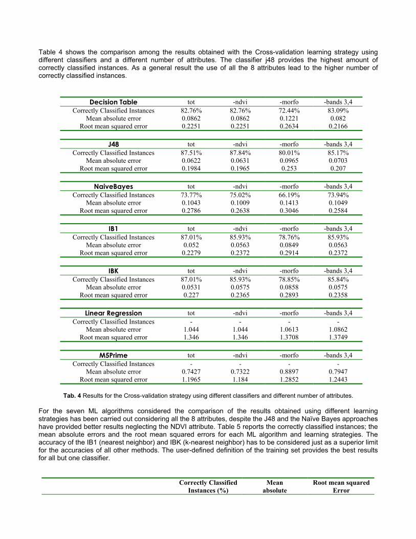
Table 4 shows the comparison among the results obtained with the Cross-validation learning strategy using different classifiers and a different number of attributes. The classifier j48 provides the highest amount of correctly classified instances. As a general result the use of all the 8 attributes lead to the higher number of correctly classified instances.

Decision Table tot -ndvi -morfo -bands 3,4 Correctly Classified Instances 82.76% 82.76% 72.44% 83.09%

Mean absolute error 0.0862 0.0862 0.1221 0.082 Root mean squared error 0.2251 0.2251 0.2634 0.2166

J48 tot -ndvi -morfo -bands 3,4

Correctly Classified Instances 87.51% 87.84% 80.01% 85.17% Mean absolute error 0.0622 0.0631 0.0965 0.0703

Root mean squared error 0.1984 0.1965 0.253 0.207

NaiveBayes tot -ndvi -morfo -bands 3,4 Correctly Classified Instances 73.77% 75.02% 66.19% 73.94%


IB1 tot -ndvi -morfo -bands 3,4

Correctly Classified Instances 87.01% 85.93% 78.76% 85.93% Mean absolute error 0.052 0.0563 0.0849 0.0563


IBK tot -ndvi -morfo -bands 3,4 Correctly Classified Instances 87.01% 85.93% 78.85% 85.84%


Linear Regression tot -ndvi -morfo -bands 3,4

Correctly Classified Instances - - - - Mean absolute error 1.044 1.044 1.0613 1.0862


M5Prime tot -ndvi -morfo -bands 3,4 Correctly Classified Instances - - - -


Tab. 4 Results for the Cross-validation strategy using different classifiers and different number of attributes.

For the seven ML algorithms considered the comparison of the results obtained using different learning strategies has been carried out considering all the 8 attributes, despite the J48 and the Naïve Bayes approaches have provided better results neglecting the NDVI attribute. Table 5 reports the correctly classified instances; the mean absolute errors and the root mean squared errors for each ML algorithm and learning strategies. The accuracy of the IB1 (nearest neighbor) and IBK (k-nearest neighbor) has to be considered just as a superior limit for the accuracies of all other methods. The user-defined definition of the training set provides the best results for all but one classifier.

Correctly Classified Instances (%)

Mean absolute

Root mean squared Error

error Cross-validation Training set

Decision Table

Percentage split

82.76 86.92 86.86

0.0862 0.0732 0.0751

0.0225 0.1913 0.2168

Cross-validation Training set

J48

Percentage split

87.51 92.42 88.02

0.0622 0.0470 0.0580

0.1984 0.1534 0.1923


NaiveBayes

Percentage split

73.77 74.44 75.55

0.1043 0.1016 0.0924

0.2786 0.2736 0.2612

IB1 Cross-validation 87.01 0.0520 0.2279 Training set 100 0.0000 0.0000 Percentage split 87.28 0.0509 0.2255


IBK

Percentage split

87.01 100

87.28

0.0531 0.0013 0.0525

0.2270 0.0017 0.2248


LinearRegression

Percentage split

- - -

1.0444 1.0390 0.9207

1.3460 1.3374 1.2477


M5Prime

Percentage split

- - -

0.7427 0.6748 0.6807

1.1965 1.0972 1.1695

Tab. 5 Results obtained for different learning strategies and different ML algorithms.

The J48 algorithm has provided the smaller errors and the analysis has therefore been continued only over this classifier, which has also been implemented/ported in GRASS to produce the final land cover map. Table 6 reports the comparison between the results obtained using the J48 classifier with different numbers of instances.

J48 Correctly Classified

Instances (%)

Mean absolute

error


1201 Cross-validation 87.51 0.0622 0.1984 Training set 92.42 0.0470 0.1534 Percentage split 88.02 0.0580 0.1923

88 Cross-validation 67.41 0.1242 0.3102 Training set 88.76 0.0595 0.1725 Percentage split 87.10 0.0719 0.2054

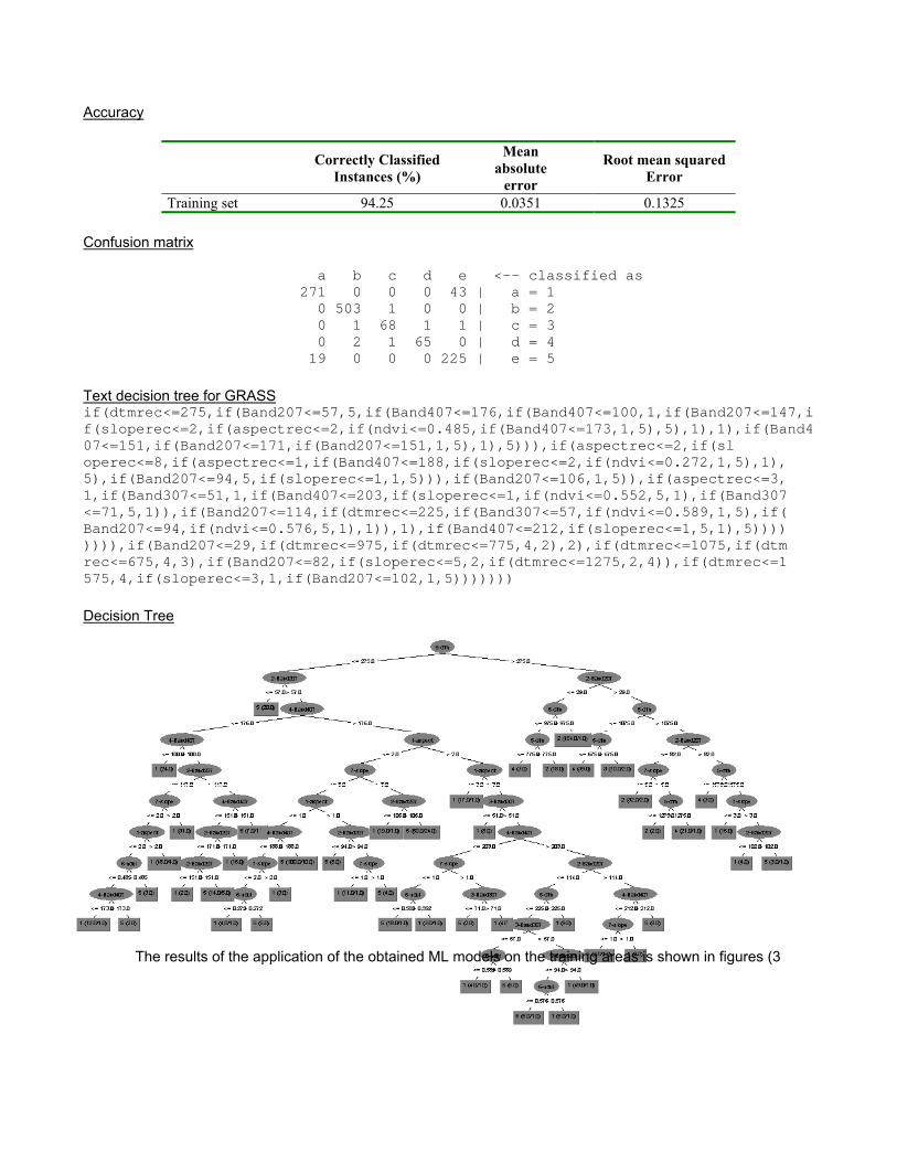
Tab. 6 Results obtained using the entire data set and a small sub-set for different learning strategies and j48 ML algorithm. The following results have been obtained dealing the 1201 instances with the classifier j48 and the Training Set learning strategy, using the Binary Splits option and setting the confidence factor to 0.01 and 0.25.

1) J48 Training Set BinarySplits=True Confidence Factor=0.01

2)J48 Training Set BinarySplits=True Confidence Factor=0.25 In the following part the graphical decision tree representation, the accuracies and confusion matrixes for both the tests are reported. Since these two classifiers have been implemented in GRASS the text form of the two decision trees has been re-written following the r.mapcalc rules. 1) J48_Training Set_BinarySplits=True_Conf.Factor=0.01

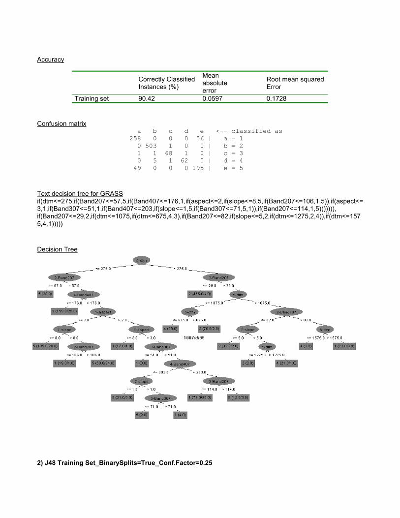
Accuracy


Mean absolute error


Training set 90.42 0.0597 0.1728 Confusion matrix

a b c d e <-- classified as 258 0 0 0 56 | a = 1 0 503 1 0 0 | b = 2 1 1 68 1 0 | c = 3 0 5 1 62 0 | d = 4 49 0 0 0 195 | e = 5

Text decision tree for GRASS if(dtm<=275,if(Band207<=57,5,if(Band407<=176,1,if(aspect<=2,if(slope<=8,5,if(Band207<=106,1,5)),if(aspect<=3,1,if(Band307<=51,1,if(Band407<=203,if(slope<=1,5,if(Band307<=71,5,1)),if(Band207<=114,1,5))))))), if(Band207<=29,2,if(dtm<=1075,if(dtm<=675,4,3),if(Band207<=82,if(slope<=5,2,if(dtm<=1275,2,4)),if(dtm<=1575,4,1))))) Decision Tree

2) J48 Training Set_BinarySplits=True_Conf.F

actor=0.25

Accuracy


Mean absolute

error


Training set 94.25 0.0351 0.1325 Confusion matrix

a b c d e <-- classified as 271 0 0 0 43 | a = 1 0 503 1 0 0 | b = 2 0 1 68 1 1 | c = 3 0 2 1 65 0 | d = 4 19 0 0 0 225 | e = 5

Text decision tree for GRASS if(dtmrec<=275,if(Band207<=57,5,if(Band407<=176,if(Band407<=100,1,if(Band207<=147,if(sloperec<=2,if(aspectrec<=2,if(ndvi<=0.485,if(Band407<=173,1,5),5),1),1),if(Band407<=151,if(Band207<=171,if(Band207<=151,1,5),1),5))),if(aspectrec<=2,if(sl operec<=8,if(aspectrec<=1,if(Band407<=188,if(sloperec<=2,if(ndvi<=0.272,1,5),1), 5),if(Band207<=94,5,if(sloperec<=1,1,5))),if(Band207<=106,1,5)),if(aspectrec<=3, 1,if(Band307<=51,1,if(Band407<=203,if(sloperec<=1,if(ndvi<=0.552,5,1),if(Band307 <=71,5,1)),if(Band207<=114,if(dtmrec<=225,if(Band307<=57,if(ndvi<=0.589,1,5),if( Band207<=94,if(ndvi<=0.576,5,1),1)),1),if(Band407<=212,if(sloperec<=1,5,1),5)))) )))),if(Band207<=29,if(dtmrec<=975,if(dtmrec<=775,4,2),2),if(dtmrec<=1075,if(dtm rec<=675,4,3),if(Band207<=82,if(sloperec<=5,2,if(dtmrec<=1275,2,4)),if(dtmrec<=1 575,4,if(sloperec<=3,1,if(Band207<=102,1,5)))))))

Decision Tree

The results of the application of the obtained ML models on the training areas is shown in figures (3

RED = URBAN AREA

YELLOW = VINEYARDS

Fig. 3 Urban area region classified using:

RIGHT J48 Training Set BinarySplits=True Confidence Factor=0.25

LEFT J48 Training Set BinarySplits=True Confidence Factor=0.01

Fig. 4 Vineyards region classified using:



YELLOW = VINEYARDS

RED = URBAN AREA

LIGHT BLUE = FOREST

GREEN = DARK FOREST

VIOLET =ROCKS

GREEN = DARK FOREST

LIGHT BLUE = FOREST

Fig. 5 Dark forest region classified using:



Fig. 6 Forest region classified using



VIOLET = ROCKS

LIGHT BLUE =

Fig. 7 Rocks and not cultivated region classified using:



The following figures show the land cover maps obtained applying both the ML models implemented in

the GIS GRASS on an unclassified region.

Fig. 8 Land cover maps produces for the entire studied zone, classified whit:



Figure 9 shows the comparison between the ortho-photo and the land cover classified map obtained with

the Confidence Factor set to 0.01.

Fig. 9 Ortho-photo image and land cover map classified with:

J48 Training Set BinarySplits=True Confidence Factor=0.01

6.Conclusions A machine learning approach to realize a land cover classification based on the integrated use of remotely sensed data and geomorphologic information has been successfully developed. In particular the information of the terrain height, aspect and slope have been used. Some of the more widely used Machine Learning algorithms have been considered and compared in terms of number of correctly classified instances, mean absolute errors and Root mean squared errors. Different strategies for the definition of the training and of the test set have, moreover, been applied. The higher accuracy has been obtained applying the J48 decision tree algorithm with an user-defined training and test set. The more important role in the classification model produced has been played by the terrain height, followed by the visible green band, the near infrared band and by the terrain aspect. Despite the relevant role of the Normalized Difference Vegetation Index (NDVI) reported in the literature in the decision trees produced is not a determinant parameter (where present in the tree it is in the lowest leave). The presence of discrete attributes with small variability in the dataset could had influenced the NDVI role in the learning procedure since its greater variability of the NDVI. The urban area and the vineyards classes present the biggest errors between predicted and apriori classified values. The differences could be reduced in further applications through the introduction of the Landsat band 1 (blue-green), band 6 (thermal-infrared) and the panchromatic image. An improvement of the classifiers performance and of the decision trees structure could be achieved through the use of a boosting algorithm. As another not-radiometric attribute, a shadow parameter, calculated with the GRASS module r.sun could be recommended.

The lack of an already classified land cover map has not allowed a quality test of the obtained map, anyway a visual comparison between the final map and the ortho-photo provides a good validation of the implemented procedure.

7. References Breimann, L., Friedmann, J., Olshen, R., Stone, C., 1984. Classification and regression trees. Wadsworth, Belmont, CA. DeFries, R., Cheung-Wai Chan, J., 2000. Multiple Criteria for Evaluating Machine Learning Algorithms for Land Cover Classification from Satellite Data. Remote Sensing of Environment, 74: 503-515. DeFries, R., Hansen, M., Townshend, J. R. G. and Sohlberg, R., 1998. Global land cover classifications at 8 km spatial resolution: The use of training data derived from Landsat imagery in decision tree classifiers. International Journal of Remote Sensing; 19 (16): 3141-3168. Džeroski, S., 2001, Data mining in a nutshell, Relational Data Mining, Springer-Verlag New York, Inc., New York, NY, GRASS development team, GRASS 5.3.x Reference Manual, http://grass.itc.it/gdp/html_grass5/index.html Han, J., Kamber, M., 2001. Data mining: concepts and techniques. Morgan Kaufmann, San Francisco, CA. Hansen, M., DeFries, R., Townshend, J. R. G. and Sohlberg, R., 2000. Global land cover classification at 1km resolution using a decision tree classifier. International Journal of Remote Sensing. 21: 1331-1365. Hogg, R.V., Creig, A.T., 1995. Introduction to mathematical statistic. 5th edition. Prentice Hall, Englewood Cliffs, NJ. Wiley, J. and Sons, 1997. Machine learning, data mining and knowledge discovery: methods and applications. Michalski, R.S., Bratko, I., Kubat, M., editors. Witten, I.H., Frank, E., 2000. Data mining: practical machine learning tools and techniques with Java implementations.

a grass-datamining integrated procedure for land cover

Documents