a globally uniformly ultimately bounded adaptive …
TRANSCRIPT
A GLOBALLY UNIFORMLY ULTIMATELY BOUNDED ADAPTIVE ROBUST
CONTROL APPROACH TO A SECOND-ORDER NONLINEAR MOTION SYSTEM
WITH INPUT SATURATION
A Dissertation
Submitted to the Faculty
of
Purdue University
by
Yun Hong
In Partial Fulfillment of the
Requirements for the Degree
of
Doctor of Philosophy
May 2008
Purdue University
West Lafayette, Indiana

ii
[To my beloved parents and husband.]

iii
ACKNOWLEDGMENTS
I would like to thank my major advisor Professor Bin Yao for his inspirational guidance
and constant support. Led by him, I have experienced a wonderful journey towards my
academic goal. He will always have my sincerest respect and deepest gratitude.
I would also like to express my genuine gratitude to Professor George Chiu, Profes-
sor Stanislaw Zak, and Professor Venkataramanan Balakrishnan for their great service as
my advisory committee. They have passed me invaluable knowledge and precious advice
through lectures and casual discussions.
During my long time graduate study, my parents and my husband have supported me
with their everlasting love, care and encouragement. They share my joyful moments and
comfort me when things don’t go well. I am also very grateful to my dear friends, lab mates
and group members. Their timeless friendship will be cherished in my memory.
This work is funded in part by National Science Foundation (NSF) Grant CMS-9734345,
CMS-0220179, CMS-0600516 and in part by the National Natural Science Foundation of
China (NSFC) Grant 50528505. The sponsorship by the Mechanical Engineering School
of Purdue University is highly acknowledged.

iv
TABLE OF CONTENTS
Page
LIST OF TABLES . . . . . . . . . . . . . . . . . . . . . . . . . . . . . . . . . vi
LIST OF FIGURES . . . . . . . . . . . . . . . . . . . . . . . . . . . . . . . . vii
ABSTRACT . . . . . . . . . . . . . . . . . . . . . . . . . . . . . . . . . . . . x
1 INTRODUCTION . . . . . . . . . . . . . . . . . . . . . . . . . . . . . . . 11.1 Background and Motivation . . . . . . . . . . . . . . . . . . . . . . . 11.2 Literature Survey . . . . . . . . . . . . . . . . . . . . . . . . . . . . . 3
1.2.1 Adaptive Robust Control (ARC) . . . . . . . . . . . . . . . . . 31.2.2 Saturation Control . . . . . . . . . . . . . . . . . . . . . . . . 41.2.3 Parameter Estimation . . . . . . . . . . . . . . . . . . . . . . 81.2.4 Dynamic Friction Compensation . . . . . . . . . . . . . . . . . 91.2.5 Control of Linear Motor Drive System . . . . . . . . . . . . . . 11
1.3 Outline of Thesis . . . . . . . . . . . . . . . . . . . . . . . . . . . . . 12
2 SATURATED ADAPTIVE ROBUST CONTROL WITH KNOWN MASS . . 142.1 Problem Formulation and Practical Assumptions . . . . . . . . . . . . . 142.2 Saturated Adaptive Robust Control (SARC) . . . . . . . . . . . . . . . 16
2.2.1 Controller Design . . . . . . . . . . . . . . . . . . . . . . . . 172.2.2 Proof of Globally Uniformly Ultimate Boundedness and Asymp-
totic Tracking . . . . . . . . . . . . . . . . . . . . . . . . . . 222.3 Saturated Desired Compensation ARC (SDCARC) . . . . . . . . . . . 30
2.3.1 Proof of Globally Uniformly Ultimate Boundedness and Asymp-totic Tracking . . . . . . . . . . . . . . . . . . . . . . . . . . 32
2.4 Hardware Experiments . . . . . . . . . . . . . . . . . . . . . . . . . . 342.4.1 System Setup . . . . . . . . . . . . . . . . . . . . . . . . . . 342.4.2 Implementation Issue and Design Parameters with SARC . . . . 352.4.3 Implementation Issue and Design Parameters with SDCARC . . 362.4.4 Real-time Experimental Results with SARC . . . . . . . . . . . 372.4.5 Comparative Experimental Results with SDCARC, SARC and PID 44
2.5 Conclusion . . . . . . . . . . . . . . . . . . . . . . . . . . . . . . . . 47
3 SATURATED ADAPTIVE ROBUST CONTROL WITH UNKNOWN MASS 563.1 Problem Formulation and Practical Assumptions . . . . . . . . . . . . . 573.2 Controller Design . . . . . . . . . . . . . . . . . . . . . . . . . . . . 583.3 Proof of Globally Uniformly Ultimate Boundedness . . . . . . . . . . . 613.4 Parameter Estimation . . . . . . . . . . . . . . . . . . . . . . . . . . . 66
v
Page3.5 Hardware Experiments . . . . . . . . . . . . . . . . . . . . . . . . . . 69
3.5.1 Point-To-Point Trajectory . . . . . . . . . . . . . . . . . . . . 693.5.2 Step-like Trajectory . . . . . . . . . . . . . . . . . . . . . . . 75
3.6 Conclusion . . . . . . . . . . . . . . . . . . . . . . . . . . . . . . . . 85
4 SYSTEM IDENTIFICATION OF THE LINEAR MOTOR DRIVE SYSTEM . 864.1 Offline Parameter Adaptation . . . . . . . . . . . . . . . . . . . . . . 864.2 Online Parameter Adaptation . . . . . . . . . . . . . . . . . . . . . . . 96
4.2.1 Gradient Type Direct Adaptation . . . . . . . . . . . . . . . . . 964.2.2 Recursive Least Squares Indirect Adaptation . . . . . . . . . . . 984.2.3 Integrated Direct/Indirect Adaptation . . . . . . . . . . . . . . 994.2.4 Comparative Experimental Results . . . . . . . . . . . . . . . . 99
4.3 Conclusion . . . . . . . . . . . . . . . . . . . . . . . . . . . . . . . . 102
5 DYNAMIC FRICTION COMPENSATION . . . . . . . . . . . . . . . . . . 1035.1 Problem Formulation . . . . . . . . . . . . . . . . . . . . . . . . . . . 1035.2 Adaptive Robust Control . . . . . . . . . . . . . . . . . . . . . . . . . 106
5.2.1 ARC Design . . . . . . . . . . . . . . . . . . . . . . . . . . . 1065.2.2 Discontinuous Projection Mapping . . . . . . . . . . . . . . . 1075.2.3 Proof of System Boundedness and Asymptotic Tracking . . . . . 108
5.3 Comparative Simulation Studies . . . . . . . . . . . . . . . . . . . . . 1095.4 Conclusion . . . . . . . . . . . . . . . . . . . . . . . . . . . . . . . . 113
6 FUTURE RESEARCH . . . . . . . . . . . . . . . . . . . . . . . . . . . . . 1176.1 The Remaining Issues with Input Saturation Problem . . . . . . . . . . 1176.2 The Remaining Issues with Dynamics Friction Compensation . . . . . . 118
LIST OF REFERENCES . . . . . . . . . . . . . . . . . . . . . . . . . . . . . 121
VITA . . . . . . . . . . . . . . . . . . . . . . . . . . . . . . . . . . . . . . . . 127
vi
LIST OF TABLES
Table Page
2.1 Performance indexes of three controllers. . . . . . . . . . . . . . . . . . . 46
3.1 Performance indexes of sarc with unknown mass. . . . . . . . . . . . . . . 85
4.1 Offline system ID: input and output signals. . . . . . . . . . . . . . . . . . 89
4.2 Nominal parameter values for linear motor. . . . . . . . . . . . . . . . . . 99

vii
LIST OF FIGURES
Figure Page
2.1 Saturation function σ1(z1). . . . . . . . . . . . . . . . . . . . . . . . . . . 18
2.2 Saturation function σ2(z2). . . . . . . . . . . . . . . . . . . . . . . . . . . 21
2.3 Design structure. . . . . . . . . . . . . . . . . . . . . . . . . . . . . . . . 22
2.4 z1− z2 phase plane and the divided sets for stability proof. . . . . . . . . . . 24
2.5 Experiment setup of linear motor system. . . . . . . . . . . . . . . . . . . 35
2.6 Point-to-point trajectory. . . . . . . . . . . . . . . . . . . . . . . . . . . . 38
2.7 Tracking error and control input (w/o disturbance). . . . . . . . . . . . . . 38
2.8 Tracking error and control input (w/1V disturbance). . . . . . . . . . . . . 39
2.9 Tracking error and control input (w/6V disturbance). . . . . . . . . . . . . 41
2.10 Tracking error and control input (in the presence of 6V disturbance). . . . . 41
2.11 Tracking error and control input (zoomed in portion at s.s). . . . . . . . . . 42
2.12 Desired position and velocity trajectory (step reference). . . . . . . . . . . . 43
2.13 Tracking error and control input (step reference). . . . . . . . . . . . . . . 44
2.14 Tracking error and control input at s.s.(step reference). . . . . . . . . . . . 45
2.15 Tracking error with no disturbance. . . . . . . . . . . . . . . . . . . . . . 48
2.16 Tracking error with no disturbance (zoomed in portion). . . . . . . . . . . . 49
2.17 Control input with no disturbance. . . . . . . . . . . . . . . . . . . . . . . 50
2.18 Tracking error with 1V disturbance. . . . . . . . . . . . . . . . . . . . . . 51
2.19 Tracking error with 1V disturbance (zoomed in portion). . . . . . . . . . . 52
2.20 Control input with 1V disturbance. . . . . . . . . . . . . . . . . . . . . . . 53
2.21 PID with 6V disturbance. . . . . . . . . . . . . . . . . . . . . . . . . . . 53
2.22 SDCARC with 6V disturbance (the whole process). . . . . . . . . . . . . . 54
2.23 SDCARC with 6V disturbance (in the presence of the disturbance). . . . . . 54
2.24 SDCARC with 6V disturbance (zoomed in portion at stead-state). . . . . . . 55

viii
Figure Page
3.1 Point-to-point trajectory for mass range (a)[3.2,12.4]. . . . . . . . . . . . . 70
3.2 Point-to-point trajectory for mass range (b)[1.5,6]. . . . . . . . . . . . . . . 71
3.3 Point-to-point trajectory for mass range (c)[1,4]. . . . . . . . . . . . . . . . 72
3.4 P2P tracking performance of mass range (a)[3.34,12.4]. . . . . . . . . . . . 73
3.5 P2P tracking performance of mass range (b)[1.5,6]. . . . . . . . . . . . . . 73
3.6 P2P tracking performance of mass range (c)[1,4]. . . . . . . . . . . . . . . 74
3.7 P2P tracking performance (zoomed in) of mass range (a)[3.34,12.4]. . . . . 75
3.8 P2P tracking performance (zoomed in) of mass range (b)[1.5,6]. . . . . . . 76
3.9 P2P tracking performance (zoomed in) of mass range (c)[1,4]. . . . . . . . 76
3.10 An example of step-like trajectory. . . . . . . . . . . . . . . . . . . . . . . 77
3.11 Step tracking performance of mass range (a)[3.34,12.4]. . . . . . . . . . . . 79
3.12 Step tracking performance (zoomed in) of mass range (a)[3.34,12.4]. . . . . 80
3.13 Step tracking performance of mass range (b)[1.5,6]. . . . . . . . . . . . . . 81
3.14 Step tracking performance (zoomed in) of mass range (b)[1.5,6]. . . . . . . 82
3.15 Step tracking performance of mass range (c)[1,4]. . . . . . . . . . . . . . . 83
3.16 Step tracking performance (zoomed in) of mass range (c)[1,4]. . . . . . . . 84
4.1 Regressors resulting from ”Normal” square wave input (10 sec and withoutload). . . . . . . . . . . . . . . . . . . . . . . . . . . . . . . . . . . . . . 90
4.2 Regressors resulting from ”Normal” square wave input (1 sec and withoutload). . . . . . . . . . . . . . . . . . . . . . . . . . . . . . . . . . . . . . 91
4.3 Modelling error resulting from ”Normal” square wave input (without load). . 92
4.4 Regressors resulting from ”Normal” square wave input (10 sec and with load). 93
4.5 Regressors resulting from ”Normal” square wave input (1 sec and with load). 94
4.6 Modelling error resulting from ”Normal” square wave input (with load). . . 95
4.7 Online parameter estimation with no load. . . . . . . . . . . . . . . . . . . 100
4.8 Online parameter estimation with 20lb load. . . . . . . . . . . . . . . . . . 101
5.1 Experiment with coulomb-viscous compensation (no disturbance). . . . . . 110
5.2 Experiment with coulomb-viscous compensation (1V disturbance). . . . . . 111
5.3 Tracking performance with dynamic model compensation. . . . . . . . . . 113

ix
Figure Page
5.4 Friction state and estimates in dynamic model. . . . . . . . . . . . . . . . . 114
5.5 Friction force and its estimate. . . . . . . . . . . . . . . . . . . . . . . . . 115
5.6 Tracking performance with dynamic friction model and direction compensa-tion. . . . . . . . . . . . . . . . . . . . . . . . . . . . . . . . . . . . . . 115
5.7 Friction state and estimates in dynamic model. . . . . . . . . . . . . . . . . 116
5.8 Friction force and its estimate. . . . . . . . . . . . . . . . . . . . . . . . . 116

x
ABSTRACT
Hong, Yun Ph.D., Purdue University, May, 2008. A globally uniformly ultimately boundedadaptive robust control approach to a second-order nonlinear motion system with inputsaturation. Major Professor: Dr. Bin Yao, School of Mechanical Engineering.
Control input saturation is an important practical problem to control engineers. This
research focuses on the synthesis of nonlinear adaptive robust controller with saturated
actuator authority for a linear motor drive system, which is subject to parametric uncer-
tainties and uncertain nonlinearities such as input disturbance as well. Globally uniformly
ultimately bounded (GUUB) stability with limited control efforts is achieved by breaking
down the overall uncertainties to state-linearly-dependent uncertainties (such as viscous
friction) and bounded nonlinearities (such as coulomb friction, cogging force and etc.) and
treating them with different strategies. Furthermore, a guaranteed transient performance
and final tracking accuracy can be obtained by incorporating the well-developed adaptive
robust control strategy and effective parameter identifier. Asymptotic output tracking is
also achieved in the presence of parametric uncertainties only. Meanwhile, in contrast to
the existing saturated control structures that are designed based on a set of transformed
coordinates, the proposed saturated controller is carried out in the actual system states,
which have clear physical meanings. This makes it much easier and less conservative to
select the design parameters to meet the dual objective of achieving GUUB stability with
limited control efforts for rare emergency cases and the local high-bandwidth control for
high performance under normal running conditions. The proposed control strategy is de-
signed under the assumption that the moving mass is known and then extended to the case
where the moving mass is unknown and online estimated. Real-time experimental results
are obtained to illustrate the effectiveness of the saturated adaptive robust control law.
The other focus of this work is on the dynamic friction compensation. Micro and nano-
technologies need precision machines that can produce motion accuracy down to nano-

xi
meter range. The objective of this research is to present an advanced adaptive robust con-
trol approach with dynamic friction compensation to achieve nanometer level positioning
accuracy for nano-manipulation type applications. In addition, the proposed control strat-
egy is applied on a linear motor drive system with a position measurement resolution less
than 1 nanometer. Simulation results will be presented to demonstrate the ultra precision
motion that can be achieved with the proposed method.
1
1. INTRODUCTION
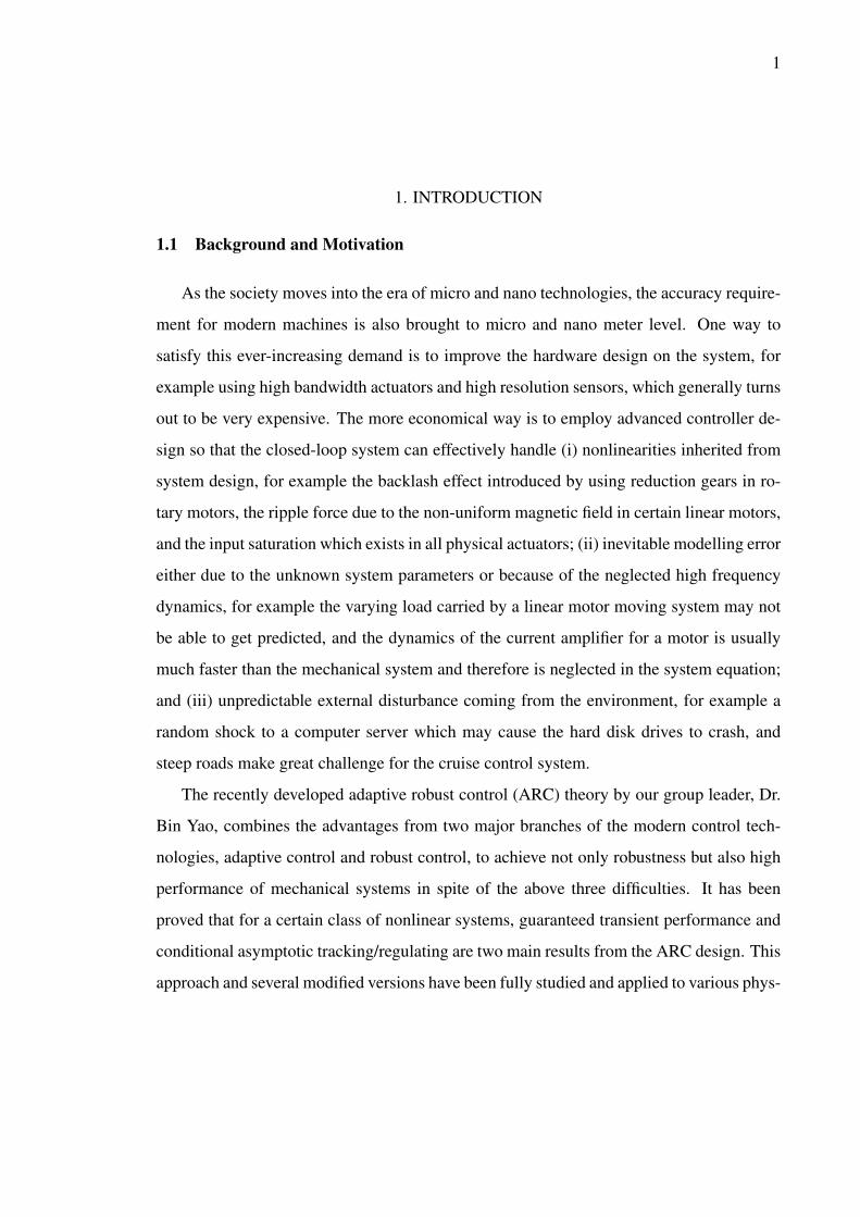
1.1 Background and Motivation
As the society moves into the era of micro and nano technologies, the accuracy require-
ment for modern machines is also brought to micro and nano meter level. One way to
satisfy this ever-increasing demand is to improve the hardware design on the system, for
example using high bandwidth actuators and high resolution sensors, which generally turns
out to be very expensive. The more economical way is to employ advanced controller de-
sign so that the closed-loop system can effectively handle (i) nonlinearities inherited from
system design, for example the backlash effect introduced by using reduction gears in ro-
tary motors, the ripple force due to the non-uniform magnetic field in certain linear motors,
and the input saturation which exists in all physical actuators; (ii) inevitable modelling error
either due to the unknown system parameters or because of the neglected high frequency
dynamics, for example the varying load carried by a linear motor moving system may not
be able to get predicted, and the dynamics of the current amplifier for a motor is usually
much faster than the mechanical system and therefore is neglected in the system equation;
and (iii) unpredictable external disturbance coming from the environment, for example a
random shock to a computer server which may cause the hard disk drives to crash, and
steep roads make great challenge for the cruise control system.
The recently developed adaptive robust control (ARC) theory by our group leader, Dr.
Bin Yao, combines the advantages from two major branches of the modern control tech-
nologies, adaptive control and robust control, to achieve not only robustness but also high
performance of mechanical systems in spite of the above three difficulties. It has been
proved that for a certain class of nonlinear systems, guaranteed transient performance and
conditional asymptotic tracking/regulating are two main results from the ARC design. This
approach and several modified versions have been fully studied and applied to various phys-

2
ical systems such as electrical-hydraulic system, linear motor drive system, piezoelectric
actuators and etc. with convincing experimental results. However, like other beautiful con-
trol designs, the ARC approach does not explicitly take the input saturation problem into
account. All the theoretic results and experimental outcomes of the ARC have a hidden as-
sumption that the designed control law can be implemented by the actuator without being
cut off by its physical limitation. We have seen in the simulation studies that the overall
system would lose stability if the input saturation is enforced on the model and gets violated
due to a very demanding desired trajectory.
Input saturation effect has already been recognized in the very early age of control
technology development. Since the classic PID control method was developed and became
more and more popular, the potential integral windup problem resulting from the use of
integral feedback and large initial error draws more and more attention from the control
community. At earlier stage, some ”ad-hoc” tricks were played to avoid input saturation.
For example, the integral action gets turned off until the tracking error is small enough. In
nowadays, more sophisticated researches have been carried out to study the system behav-
ior and maintain the stability when it runs into saturation. In our research group, a great
deal of effort has been made to study the input saturation problem under the framework
of ARC design. Meanwhile, for a system under normal working condition, developing a
more precise model is always a good direction to look into in order to improve the tracking
performance. Obtaining accurate online parameter estimation definitely reduces the model
uncertainties. On the other hand, some nonlinear dynamics is very difficult to model, such
as Coulomb friction. The commonly used sign function model may not be good enough for
nano-scale application. All these issues indicate that there is still plenty of room to make
new discovery and progress on the ARC design and its applications. Therefore, it is ben-
eficial to review previous work in all these fields: adaptive robust control design, control
input saturation, parameter estimation, friction compensation, and linear motor system.

3
1.2 Literature Survey
1.2.1 Adaptive Robust Control (ARC)
Modern control technologies can be categorized into several trends. Adaptive control
and robust control are two of the most important trends. The first strategy essentially em-
ploys a learning mechanism, either by estimating unknown system parameters online or
updating the control parameters based on past information, to reduce model uncertainty
and achieve better performance. Books [1–3] and [4] provide great resource on all kinds
of designs and applications of the adaptive control. The most known shortcoming of this
approach in general is the lack of robustness to unmodelled uncertainties and external dis-
turbance. A great deal of effort has been made to strengthen the stability of adaptive control
systems. For example, robust adaptive control was developed in [5] to consider bounded
uncertainties. In [6–8], a back-stepping design was developed for adaptive control of cer-
tain nonlinear systems and the robustness of the controlled system has been established
against uncertainties with matching (extended matching) condition.
On the other hand, the second trend focuses on using robust feedback to dominate
various model uncertainties and attenuate the resulting error [9]. Sliding mode control [10]
and H∞ control [11] are two examples of designing such a robust feedback. Book [12]
offers an insightful approach to robust control that reflects the history and most recent
developments in the field. However, since no attempt is made to learn the system in control
process, the best performance achievable is to reduce the error within certain level. The
asymptotic tracking performance which could result from adaptive control when there is
only parametric uncertainty present is never going to happen with robust control using finite
gain or finite control power.
In summary, these two major modern control trends have their own pros and cons which
actually perfect each other. The adaptive robust control design [13, 14] was developed
intending to intelligently combine the advantages of both approaches and to achieve the
desirable properties – learning ability and robustness from each side. By adopting the on-
line parameter adaptation from adaptive control, the ARC can reduce modelling error and

4
achieve asymptotic tracking when only parametric uncertainty is present. By applying ro-
bust feedback which dominates the lumped modelling error and unmodelled dynamics, the
ARC can deliver guaranteed transient performance and pre-set final tracking error. The
bridge to connect the adaptive learning mechanism and bounded robust feedback is the use
of projection mapping on the parameter estimation law, which guarantees the boundedness
of all the signals forming the control input. Several extended algorithms were developed
to further improve the performance. The research work in [15] used the pre-calculated
desired trajectory to form the model compensation term and the parameter adaptation law.
Due to significant reduced noise level, higher robust gain could be utilized and smaller final
tracking error is resulted. The algorithms proposed in [16, 17] separate the controller de-
sign with the parameter adaptation law and achieve accurate online estimation besides high
tracking performance. In addition, articles [18, 19] summarize the essences of various ver-
sions of ARC design and discuss certain issues related to hardware implementation. Under
this framework, the saturated adaptive robust control (SARC) is developed to actively take
the input saturation effect into account so that the controlled system not only preserves the
two desirable results from the ARC under normal working condition but also maintains
GUUB stability when the actuator gets saturated and quickly regains high performance
after recovering from saturation.
1.2.2 Saturation Control
All actuators of physical devices are subject to amplitude saturation. Although in some
applications it may be possible to ignore this fact, the reliable operation and acceptable
performance of most control systems must be assessed in light of actuator saturation [20].
Recent analysis on the behavior of systems with input saturation could be found in [21,22].
Lots of research works have been done to stabilize the system while taking into account
the saturation nonlinearities at the controller design stage. In [23], the author described the
phenomenon of integrator windup and various ways of avoiding it, including a number of
ad hoc schemes. Book [24] provides detailed discussion and rigorous theoretical derivation
5
for control of certain class of linear systems with input saturation. It was proved in [25]
that global stabilization is not possible using linear feedback laws for general linear sys-
tems subject to input saturation. A low-and-high gain method was used in [26] and [27] to
provide semi-global stability as well as meeting performance such as disturbance rejection,
robustness and so on for asymptotically null controllable linear systems. Some of those re-
sults were extended with global stability in [28]. Global stability results were also obtained
in [29,30] with the use of observer. For the same class of systems as in [27], robust control
techniques such as H-infinity was employed in [31] to achieve global stability but with the
difficulty to obtain a closed form expression of the solution for high-dimensional systems.
A novel saturated control structure was proposed in [32] to ensure the globally asymptotic
stability for a chain of integrators of arbitrary order by intelligently using a set of linear
coordinate transformations and multiple saturation type functions such as sigmoidal func-
tions. By the same author, semi-global stability was also achieved in [33] for linear null
controllable systems.
The model predictive control (MPC) [34] establishes a unified framework dealing with
constraints either on output, states or control input. Therefore, a lot of researches adopt the
MPC design to attack the control saturation problem such as in [35–37]. In [38], the use
of command governor strategy was investigated to deal with real control problems and this
technique was applied to an inverted pendulum system with input saturation. The study
in [35] employed another popular optimal control tool – the linear matrix inequality (LMI)
introduced by [39]. Articles [40, 41] proposed LMI-based anti-windup augmentation for
stable linear system. In [42], the authors studied robust stability of uncertain linear systems
subject to actuator saturation by using successive LMI relaxations. In [43], closed-loop
induced L2 control under the linear parameter-varying control framework was thoroughly
investigated. The researches reported in [44–46] are examples of another line of the work.
Under this framework, the control law was designed ignoring the fact of input saturation
and an anti-windup bumpless transfer (AWBT) compensation was brought to minimize the
adverse effect of the saturation.

6
In the majority of the works mentioned above, the systems under treatment are mostly
linear and exactly known, which is not the case for most physical systems in reality. It is not
unusual that some of the system parameters are unknown or their values may vary from time
to time. The idea of adaptive control is adopted to deal with the uncertain linear systems
with input saturation. For example in [47] the model uncertainty was treated by using the
model reference adaptive control. In [48], the authors proposed a new adaptive algorithm to
stabilize the system locally without assuming open loop stability and [49] is the discretized
version of [48]. The research reported in [50] promoted the design of switching controllers
to achieve high performance. The concept of ”allowed over-saturation” was proposed to
exploit the full input authority in the control law.
Nonlinear factors such as friction affect system behavior significantly and are rather
difficulty to model precisely. Therefore, it is of practical importance to expand the research
field to nonlinear systems when attacking the actuator saturation problem. The work in [51]
focused on solving the tracking control of a class of nonlinear systems with continuous-
time predictive control approach. Dr. Hedrick’s research group [52] proposed a dynamic
surface control structure as an alternative of the standard back-stepping design and used
it to quadratically stabilize the nonlinear system. Our research group [53] combined the
wise use of saturation functions proposed in [32] with the adaptive robust control (ARC)
strategy proposed in [14, 18] to achieve both the global stability and the high performance
for a chain of integrators subject to matched parametric uncertainty and uncertain nonlin-
earities. However, like the saturated controller in [32], the design is based on the set of
transformed coordinates, in which the effect of model uncertainties immediately shows up
at the beginning stage of the controller design, even though the model uncertainties are of
matched type. As a result, the extent of model uncertainties allowable in the design is much
limited, leading to a conservative overall design.
In this study, a new saturated control structure based on the back-stepping design [8]
and the ARC strategy [14, 18] is proposed [54, 55]. It has been shown in [56] that the orig-
inal ARC can achieve high tracking accuracy (close to the resolution level) under nominal
working condition. As to the stability issue, the projection-type adaptation of ARC pre-

7
vents integral windup caused by parameter adaptations. However, it does not guarantee
global stability; the position feedback functions like an integral feedback for velocity loop
which is immediately affected by the control input. Conventional ARC does not deal with
the control saturation problem caused by large position error (one can think it as an integral
windup problem for velocity feedback loop), as opposed to what the proposed controller is
able to handle. Essentially, a bounded virtual control law is designed to ensure the bound-
edness and convergence of the error signal at each step. The actual control input comes
from the design at the last step, consisting of a model compensation term whose bound
is calculable due to the pre-known information of the system and the desired trajectory,
and a locally-high-gain-globally-saturated robust control term to meet the dual objective
of achieving global stability with limited control efforts for rare emergency cases and the
local high-bandwidth control for high performance under normal running conditions. To
better illustrate the essential idea and the high performance nature of the proposed satu-
rated ARC control strategy in practical applications, the precision control of a positioning
system driven by linear motors is considered. The same set of equipment has also been
used to test the design in [53]. However, unlike [53], the proposed saturated ARC design is
based on the actual system states, in which state equations do not have model uncertainties
except the last one due to the nature of matched model uncertainties of these systems [56].
As such, there is no need to consider the effect of model uncertainties until the last step
of the design, removing the design conservativeness of [53]. Furthermore, the clear physi-
cal meaning of the actual system states makes it easier and more straightforward to select
and tune the controller design parameters in implementation. All these make the proposed
saturated ARC controller a more practical solution to the saturated actuator problem while
without losing high performance under normal running conditions. Experimental results
will be provided to confirm these claims.

8
1.2.3 Parameter Estimation
System identification refers broadly to the problem of developing a mathematical de-
scription of the real system based on input output data. In general there are three types of
methods to build mathematical models under different situations: black box, white box and
grey box. Black box is for those systems with which only input output data are available. If
the system is linear time-invariant, the frequency response could be generated based on the
output signals excited by a sweep of sine waves over a frequency range of interest. By ana-
lyzing the frequency response, a great deal of information could be obtained to identify the
system. White box is for those systems whose dynamics is easy to derive by following the
Newton laws with all the parameters given or calculable. The third one – grey box method
is more often to apply. In this case, part of the model could be generated directly by fol-
lowing physical principles such as its structure; whereas the other part such as the system
parameters needs input output signals obtained from real-time experiments to estimate and
complete the model description. Numerous lectures and books are delivered addressing the
topic of system identification such as [57] and various estimation algorithms are developed
to identify the unknown system parameters for different applications [1–3, 58].
The key condition for effective parameter estimation is the persistence excitation (PE)
condition [59]. The relationship between the PE condition and the convergence of the
estimates has been well studied in [2, 3, 60].
One of the applications of system identification is to online estimate parameters either
to reduce modelling error and tracking error for control purpose or to get accurate estima-
tion for diagnostic purpose. Depending on the emphasis of the application and considering
the computational burden, the adaptation laws can be categorized into direct [61] and in-
direct method [16]. In this work, the direct method is firstly applied to the saturated ARC
(SARC) design with known mass. When the SARC is generalized to the case where the
mass is unknown, accurate mass estimate obtained online is desirable and thus the inte-
grated direct/indirect adaptation law [17] is employed to satisfy the need. A whole chapter

9
is devoted to the system identification process of the linear motor drive system. Several im-
plementation issues rarely mentioned in literature have been discussed with great details.
1.2.4 Dynamic Friction Compensation
Friction exists in machines incorporating parts with relative motion and it is generally
an obstacle for control engineers due to its high nonlinearity and the negative results it
causes, such as steady state errors and limit cycle. Articles [62, 63] and [64] provided not
only an extensive survey of numerous studies and researches from several disciplines to ex-
plain or model the friction phenomena, but also a great insight on the applications of some
friction models to typical control problems. For example, the classical Coulomb-viscous
model, because of its simplicity, has often been used in friction compensation. As the de-
mands for precision control increase, more focus has been drawn on dynamic models for
its better description at low speed motions, where the presliding displacement, the friction
lag and the Stribeck effect, etc. become dominant. A lot of researchers have proposed
various dynamic friction models. For example, Dahl [65] modelled the stress-strain curve
by a differential equation, which is a generalization of ordinary Coulomb friction. Haessig
and Friedland [66] introduced a bristle model to capture the behavior of the microscopical
contact points between two surface. Canudas de Wit et al. [67] developed a model which
was based on the average behavior of the bristles and it combined the stiction effect with
arbitrary steady-state friction characteristics.
The idea behind obtaining these highly accurate and sophisticated models is to be able
to predict the friction more accurately so that friction compensation can be done more
effectively. However, no matter how accurate these mathematical models may be, it is
usually difficulty to capture the nonlinear features of friction exactly, since almost every
physical system is subject to certain degrees of model uncertainties. Normally, the causes
of model uncertainties can be classified into three categories: (i) repeatable or constant
unknown quantities such as the unknown dynamic friction parameters and inertia load, (ii)
dynamic uncertainties due to the unmeasurable friction state, and (iii) non-repeatable un-

10
known quantities such as external disturbances and imprecise modelling of certain physical
terms.
To account for these uncertainties, nonlinear control methods have been studied during
past years. Deterministic robust controllers (DRC) can achieve a guaranteed transient per-
formance and final tracking accuracy in the presence of parametric uncertainties, dynamic
uncertainties and uncertain nonlinearities. However, since no attempt is made to learn from
past behavior, the design is conservative and may involve either switching or infinite-gain
feedback [68, 69] for asymptotic tracking. Adaptive controllers (AC) are able to achieve
asymptotic tracking in the absence of uncertain nonlinearities without resorting to infinite
gain feedback. For example in [70], information about the friction learned from past repet-
itive motion was used for model compensation. In [71], Canudas de Wit et al. illustrated
how the control structure proposed in [67] could be modified to adapt for selected unknown
friction parameters. One adaptive controller was proposed to adapt for a single parameter
associated with normal force variation while the second one was proposed to adapt for an-
other parameter associated with temperature variation. In [72], an adaptive controller with
several deigns of observers/filters, was proposed to handle non-uniform variations in the
friction force by assuming independent coefficient change as temperature varies. Similar
result was achieved in [73], in which a dual-observer structure was utilized to estimate
different nonlinear effects of the unmeasurable friction state. However, these adaptive con-
trollers suffer from two main drawbacks - unknown transient performance and possible
non-robustness to disturbances. In [74], a robust adaptive friction compensation scheme
based on the smooth projection mapping was proposed. This scheme guarantees arbitrary
disturbance attenuation. However, it is assumed that one dynamic friction parameter is
known. Otherwise, asymptotic tracking could not be guaranteed.
In [75], a dynamic friction compensation strategy was proposed for the position track-
ing of a second order mechanical system by utilizing the idea of adaptive robust control
(ARC) [13,14,18]. By exploiting practically reasonable prior information on physical sys-
tems such as the bounds of parameter variations and the unmeasurable friction state as
much as possible, the proposed scheme effectively combined the design methods of DRC

11
and AC. Specifically, based on the available bounds on the unmeasurable friction state,
the widely used discontinuous projection mapping was utilized to modify the observer de-
sign proposed in [73], which guarantees that the friction state estimates belong to a known
bounded region all the time. As a result, the possible destabilizing effect of friction state
estimation errors could be dealt with via robust feedback effectively for an improved per-
formance. The proposed controller was robust to unknown mechanical parameters and
external bounded disturbance. In the absence of uncertain nonlinearities, asymptotic out-
put tracking was achieved in spite of parametric uncertainties that may exist in the system
and dynamic friction model. However, [75] presented only simulation results. No real-time
experiments has been done due to the lack of high-resolution encoder. Therefore, it is still
under question that how effective the dynamic friction compensation will be on a real sys-
tem with sampling effect, disturbance from the working environment, neglected electrical
dynamics, etc. In this work, a new linear motor drive system is set up with the position
resolution up to nanometer scale, which can clearly show the friction effect during slow
motions if not well compensated. Preliminary test results have been obtained from the
hardware system [76]. In addition, one more parameter is added for adaptation to account
for the low frequency component of the lumped modelling error and disturbance. Design
parameters are also modified to achieve optimal performance. A simulation comparison
between the compensators with two friction models – the classical Coulomb-viscous VS.
dynamic model is made to demonstrate the advantage of the proposed scheme.
1.2.5 Control of Linear Motor Drive System
Generally, linear motions are realized by rotary motors with mechanical transmission
mechanism such as reduction gears or lead screw, which slows down the dynamic response
and introduces nonlinearities such as backlash to the system. Therefore this transmission
mechanism puts a hard limit on the closed-loop response the overall system can achieve
even with a well designed controller. As an alternative, linear motors eliminate the mechan-

12
ical transmission part, thus they have a promising potential for high speed high accuracy
positioning systems [77–79].
On the other hand, since the working principle of linear motor systems is in general to
generate driving force by the electro-magnetic relationship, certain nonlinearities related
to the magnetic field will be introduced to the system and reflected on the motion of the
moving stage. For example, the iron core linear motor is expected to have significant ripple
force and cogging force due to the open and non-uniform magnetic field. Therefore, a well
designed control law which can take care these nonlinearities is desirable in order to make
good use of the high performance potential of linear motor systems.
A lot of researches by other groups have been studying the precision motion control
of the linear motor systems [77–82]. Various kinds of techniques such as H∞ control,
disturbance observer, feedforward compensation, offline system identification and etc. have
been investigated and applied to achieve system stability and high performance.
A precision X-Y table with two different kinds of linear motor systems have been set
up in our research lab. The Y-axis is driven by an Anorad LEM-S-3-S linear motor with
epoxy core whereas the X-axis is driven by an Anorad LCK-S-1 linear motor with iron
core. They represent the two most popularly used linear motors with different character-
istics. The adaptive robust control algorithm and its extended versions have been applied
to this test bed and numerous experimental results have been produced to demonstrate the
effectiveness of the ARC [56, 83–88]. The work in this thesis use the Y-axis linear motor
system as a case of study.
1.3 Outline of Thesis
The rest of the thesis is organized as follows. The linear motor drive system serves as a
case of study throughout the whole thesis. Chapter 2 studies the saturation control problem
assuming that the mass of the stage is given or could be calculated in advance. Two main
results from the controller design – globally uniformly ultimately boundedness (GUUB)

13
and asymptotic tracking are claimed and proved. Comparative experimental results are
provided to confirm the claims.
In Chapter 3, the assumption on the system mass is relaxed. The input saturation prob-
lem is revisited with the unknown mass. Guaranteed stability is proved for the closed-loop
system and significant improvement on the performance could be observed after the mass
estimate is obtained. The proposed control method is then applied on the physical system
to show its effectiveness.
Getting quick and accurate mass estimate is the key to the success of the control strat-
egy introduced in Chapter 3. Chapter 4 elaborates on this topic and describes the system
identification process of the linear motor drive system. Extensive tests have been carried
out and the results are provided to help tell the story.
Chapter 5 introduces another way to improve the system performance by applying a
better model to describe the friction force. Adaptive robust control designed based on
the dynamic friction model is applied to the linear motor system. Since the resolution of
the position sensor is not high enough, only simulation results are available to show the
performance improvement over the ARC based on the Coulomb-viscous friction model.
There are several unsolved issues with each chapter mentioned above and Chapter 6
discusses and summarizes those issues. Suggestions are made for the future work.

14
2. SATURATED ADAPTIVE ROBUST CONTROL WITH KNOWN MASS
In this chapter, a linear motor drive system is used as a case of study. The mass of the
moving stage plus load is assumed to be known. The amplitude of the control input to
the motor is limited. A control design incorporating certain saturation function and the
well-developed ARC scheme, named saturated adaptive control (SARC), is synthesized to
deal with the input saturation effect. The closed-loop system can achieve tracking perfor-
mance with good accuracy and robustness under nominal working condition and proved to
be globally uniformly ultimately bounded (GUUB) in the presence of impulsive external
disturbance. Based on SARC, certain modifications are made to address the noise effect
since the velocity feedback used in the algorithm is obtained via numerical method and
the introduced noise not only reduces the tracking accuracy, but also limits the choice of
the control/adaptive gain. The new algorithm, saturated desired compensation ARC (SD-
CARC), can improve the tracking performance and guarantee the GUUB as well. Compar-
ative experiments are carried out and the results validate the above claims.
2.1 Problem Formulation and Practical Assumptions
The linear motor used as a case study is a current-controlled three-phase epoxy core
motor, which drives a linear positioning stage supported by recirculating bearings. Let x1
and x2 represent the stage position and velocity respectively, and x = [x1,x2]T be the state
vector. In order to capture the essential dynamics, the system model includes both viscous
and Coulomb friction, the latter of which has a highly nonlinear effect approximated by the
function FscS f (x2) as in [56]; Fsc represents the magnitude and S f (x2) is a non-decreasing
continuous function that approximates the discontinuous sign function sgn(x2) which is
15
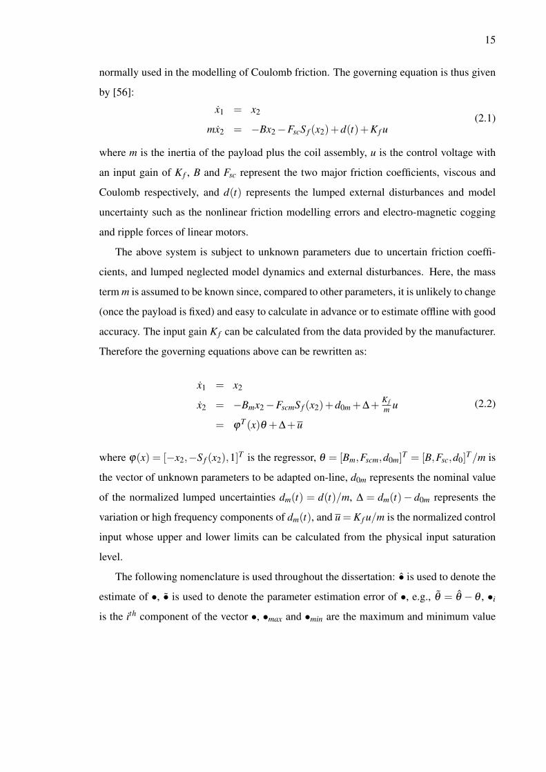
normally used in the modelling of Coulomb friction. The governing equation is thus given
by [56]:
x1 = x2
mx2 = −Bx2−FscS f (x2)+d(t)+K f u(2.1)
where m is the inertia of the payload plus the coil assembly, u is the control voltage with
an input gain of K f , B and Fsc represent the two major friction coefficients, viscous and
Coulomb respectively, and d(t) represents the lumped external disturbances and model
uncertainty such as the nonlinear friction modelling errors and electro-magnetic cogging
and ripple forces of linear motors.
The above system is subject to unknown parameters due to uncertain friction coeffi-
cients, and lumped neglected model dynamics and external disturbances. Here, the mass
term m is assumed to be known since, compared to other parameters, it is unlikely to change
(once the payload is fixed) and easy to calculate in advance or to estimate offline with good
accuracy. The input gain K f can be calculated from the data provided by the manufacturer.
Therefore the governing equations above can be rewritten as:
x1 = x2
x2 = −Bmx2−FscmS f (x2)+d0m +∆+ K fm u
= ϕT (x)θ +∆+u
(2.2)
where ϕ(x) = [−x2,−S f (x2),1]T is the regressor, θ = [Bm,Fscm,d0m]T = [B,Fsc,d0]T /m is
the vector of unknown parameters to be adapted on-line, d0m represents the nominal value
of the normalized lumped uncertainties dm(t) = d(t)/m, ∆ = dm(t)− d0m represents the
variation or high frequency components of dm(t), and u = K f u/m is the normalized control
input whose upper and lower limits can be calculated from the physical input saturation
level.
The following nomenclature is used throughout the dissertation: • is used to denote the
estimate of •, • is used to denote the parameter estimation error of •, e.g., θ = θ − θ , •i
is the ith component of the vector •, •max and •min are the maximum and minimum value

16
of •(t) for all t respectively. The following practical assumptions are made for the system,
which could be regarded as given information.
Assumption 1: The extents of the parametric uncertainties are known, i.e.,
Bm ∈ [Bml,Bmu],Fscm ∈ [Fscml,Fscmu]
where Bml , Bmu, Fscml , Fscmu are known.
For any controller to be able to stabilize the system even locally, the actuator has to be
physically powerful enough to withstand the external disturbances. As such, only bounded
disturbances will be considered, which leads to the following assumption:
Assumption 2: The lumped uncertainty dm(t) is bounded, i.e.,
|dm(t)| ≤ δdm
where δdm is known.
With the above assumptions,it is obvious that the parameter vector θ belongs to a set Ωθ
as θ ∈Ωθ = θmin≤ θ ≤ θmax, where θmin = [Bml,Fscml,−δdm]T , θmax = [Bmu,Fscmu,δdm]T ;
the operation ≤ for two vectors is performed componentwise. The desired position x1d(t),
velocity x2d(t) = x1d(t) and acceleration x1d(t), are assumed to be known and bounded. Let
ubd represent the normalized bound of the actuator authority. The saturation control prob-
lem can be stated as: under the above assumptions and the normalized input constraint
of |u(t)| ≤ ubd , design a control law that globally stabilizes the system and minimizes the
output tracking error z1 = x1− x1d(t).
2.2 Saturated Adaptive Robust Control (SARC)
In this section, a saturated adaptive robust controller (ARC) will be presented to solve
the above saturated control problem while pushing the achievable practical control perfor-
mance to the limit.

17
2.2.1 Controller Design
The proposed saturated ARC design follows the standard back-stepping design proce-
dure [8] as follows.
From (2.1), z1 = x2− x1d(t). The first step is to synthesize a bounded virtual control
law α1 for x2 so that the output tracking error z1 converges to zero globally when x2 = α1.
For this purpose, denoting the actual input discrepancy as z2 = x2−α1, then z1 dynamics
becomes:
z1 = z2 +α1− x1d (2.3)
The saturated adaptive robust control (SARC) law for α1 is proposed as:
α1 = α1a +α1s, α1a = x1d, α1s =−σ1(z1) (2.4)
where σ1(z1) is designed to be a smooth (first-order differentiable), non-decreasing, satu-
ration function with respect to z1 and it has the following four properties:
(i) If |z1|< L11, then σ1(z1) = k1z1.
(ii) z1σ1 > 0, ∀z1 6= 0.
(iii) |σ1(z1)| ≤M1,∀z1 ∈ R.
(iv) |∂σ1∂ z1| ≤ k1 if |z1|< L12, and |∂σ1
∂ z1|= 0 if |z1| ≥ L12.
Graphically, such a saturation function can be drawn as in Fig. 2.1 and L11, L12, k1, M1
are the positive design parameters to be specified in detail later. With (2.4), (2.3) becomes
z1 = z2−σ1(z1) (2.5)
which guarantees z1 −→ 0 globally when z2 = 0. So let us look at the dynamics of z2:
z2 = x2− α1 = ϕT (x)θ +∆+u− x1d +∂σ1
∂ z1(z2−σ1) (2.6)

18
Figure 2.1. Saturation function σ1(z1).
19
Let u = ua +us in which ua represents the model compensation and us for robust term. The
idea is to use ua to compensate for the known part of the model dynamics for perfect track-
ing and us to fight against various model uncertainties including the external disturbances.
In addition, both ua and us should be designed to be bounded to make sure that u stays
within its saturation limits. The details are given below.
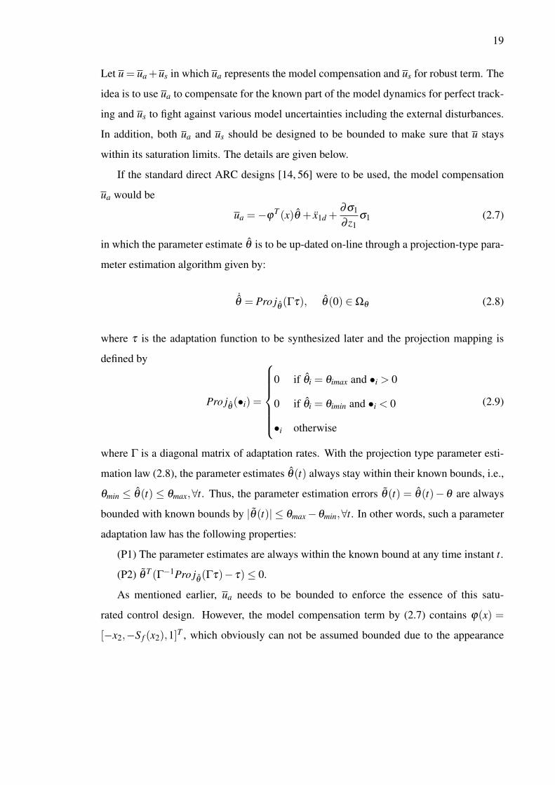
If the standard direct ARC designs [14, 56] were to be used, the model compensation
ua would be
ua =−ϕT (x)θ + x1d +∂σ1
∂ z1σ1 (2.7)
in which the parameter estimate θ is to be up-dated on-line through a projection-type para-
meter estimation algorithm given by:
˙θ = Pro jθ (Γτ), θ(0) ∈Ωθ (2.8)
where τ is the adaptation function to be synthesized later and the projection mapping is
defined by
Pro jθ (•i) =
0 if θi = θimax and •i > 0
0 if θi = θimin and •i < 0
•i otherwise
(2.9)
where Γ is a diagonal matrix of adaptation rates. With the projection type parameter esti-
mation law (2.8), the parameter estimates θ(t) always stay within their known bounds, i.e.,
θmin ≤ θ(t) ≤ θmax,∀t. Thus, the parameter estimation errors θ(t) = θ(t)−θ are always
bounded with known bounds by |θ(t)| ≤ θmax−θmin,∀t. In other words, such a parameter
adaptation law has the following properties:
(P1) The parameter estimates are always within the known bound at any time instant t.
(P2) θ T (Γ−1Pro jθ (Γτ)− τ)≤ 0.
As mentioned earlier, ua needs to be bounded to enforce the essence of this satu-
rated control design. However, the model compensation term by (2.7) contains ϕ(x) =
[−x2,−S f (x2),1]T , which obviously can not be assumed bounded due to the appearance
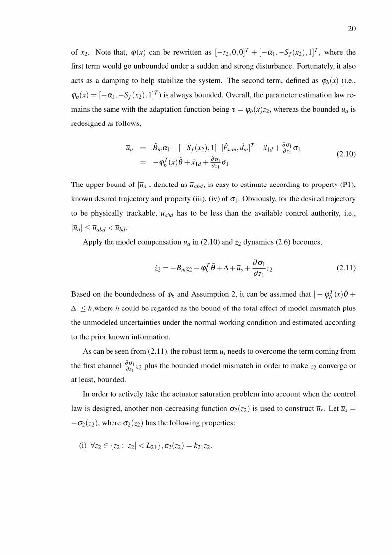
20
of x2. Note that, ϕ(x) can be rewritten as [−z2,0,0]T + [−α1,−S f (x2),1]T , where the
first term would go unbounded under a sudden and strong disturbance. Fortunately, it also
acts as a damping to help stabilize the system. The second term, defined as ϕb(x) (i.e.,
ϕb(x) = [−α1,−S f (x2),1]T ) is always bounded. Overall, the parameter estimation law re-
mains the same with the adaptation function being τ = ϕb(x)z2, whereas the bounded ua is
redesigned as follows,
ua = Bmα1− [−S f (x2),1] · [Fscm, dm]T + x1d + ∂σ1∂ z1
σ1
= −ϕTb (x)θ + x1d + ∂σ1
∂ z1σ1
(2.10)
The upper bound of |ua|, denoted as uabd , is easy to estimate according to property (P1),
known desired trajectory and property (iii), (iv) of σ1. Obviously, for the desired trajectory
to be physically trackable, uabd has to be less than the available control authority, i.e.,
|ua| ≤ uabd < ubd .
Apply the model compensation ua in (2.10) and z2 dynamics (2.6) becomes,
z2 =−Bmz2−ϕTb θ +∆+us +
∂σ1
∂ z1z2 (2.11)
Based on the boundedness of ϕb and Assumption 2, it can be assumed that |−ϕTb (x)θ +
∆| ≤ h,where h could be regarded as the bound of the total effect of model mismatch plus
the unmodeled uncertainties under the normal working condition and estimated according
to the prior known information.
As can be seen from (2.11), the robust term us needs to overcome the term coming from
the first channel ∂σ1∂ z1
z2 plus the bounded model mismatch in order to make z2 converge or
at least, bounded.
In order to actively take the actuator saturation problem into account when the control
law is designed, another non-decreasing function σ2(z2) is used to construct us. Let us =
−σ2(z2), where σ2(z2) has the following properties:
(i) ∀z2 ∈ z2 : |z2|< L21,σ2(z2) = k21z2.

21
(ii) ∀z2 ∈ z2 : L21 ≤ |z2| ≤ L22, ∂σ2∂ z2
≥ k21,σ2(L22) = M2 and σ2(−L22) =−M2.
(iii) ∀z2 ∈ z2 : |z2|> L22, |σ2(z2)| ≥M2.
Notice this is the last channel of the system and us is a part of the real control input,
therefore σ2(z2) only needs to be continuous instead of smooth. Fig. 2.2 shows an example
of σ2(z2) that has all the required properties. The design parameters are L21, k21, L22, k22.
The complete form of control input is thus as follows:
u =−ϕTb θ + x1d + ∂σ1
∂ z1σ1−σ2(z2) (2.12)
Figure 2.2. Saturation function σ2(z2).
Remark 1 Notice that σ2(z2) has two regions with different gains whereas σ1(z1) only
has one linear gain. This is due to the fact that the model mismatch and uncertainties only
appear in z2 dynamics. The region with moderate gain k21 represents the normal operation
of the system and is selected to achieve high performance such as short transient periods
and small tracking errors while remaining insensitive to noise effects. When |z2| is between

22
L21 and L22, for example during the transient period or when model mismatch is large, more
aggressive gain k22 is employed to improve the disturbance rejection. This high gain k22
could also be designed as certain nonlinear function to achieve further improvement. When
some emergence happens, such as an overpowering random strike on the positioning stage
that drags system states far away from the normal operation region, i.e.|z2| À L22, σ2 is a
constant, so that the overall control effort is always guaranteed to stay within the physical
limit of the actuator. When the impulsive disturbance is disappears, the proposed control
strategy can pull the state back to the nominal working range and regain high performance
as proved in the following section. Or, for better transient performance, no upper bound
is imposed on σ2 and when large error occurs, just let the actuator get saturated since no
integral action is introduced to this part of the control law.
In summary, the overall design structure is illustrated as Fig. 2.3
Figure 2.3. Design structure.
2.2.2 Proof of Globally Uniformly Ultimate Boundedness and Asymptotic Tracking
Combine (2.5) and (2.11), the error dynamics can be rewritten as follows:
z1 = z2−σ1(z1)
z2 = −Bmz2−ϕTb (x)θ +∆+ ∂σ1
∂ z1z2−σ2(z2)
(2.13)

23
Before the evolutions of z1 and z2 are analyzed in details, the following constraints
on the controller design parameters are enforced in order to guarantee the GUUB of the
controlled system: (a1) k21 > k1, (b1) k1L11 > L22, (c1) h < M2−k1M1, and (d1) M2≤ ubd−uabd . The essential idea to prove the GUUB of such a system is to divide the plane into four
sets and analyze the error dynamics in each set. The conclusion is that no matter where the
initial state starts, the trajectory will reach the invariant set Ωc = z1,z2 : |z1| ≤ L11, |z2| ≤L22 in finite time with the upper bound of the reaching time estimated accordingly.
Remark 2 The above constraints (a1)–(d1) are the minimum requirements that the con-
trol parameters have to satisfy in order to make the system GUUB. Further research can be
done to explore the flexibility of choosing controller parameters given the above constraints
to optimize the achievable performance.
Theorem 2.2.1 With the proposed controller (2.4) with (2.12) satisfying conditions (a1)–
(d1), all signals are bounded. Furthermore, the error state [z1,z2]T reaches the invariant
set Ωc = z : |z1| ≤ L11, |z2| ≤ L22 in a finite time and stay within thereafter. At steady
state, the final tracking error is bounded above as |z1(∞)| ≤min hk1(k21−k1)
,L22. 4
Proof: Because of conditions (b1) and (c1), there exist positive ε1,ε2 and ε3, such that
h+ k1(M1 + ε1)+ ε2 < M2 and L22 + ε3 < k1L11. Notice that M1 > k1L11 > L22, as shown
in Fig. 2.4, the entire z1-z2 plane is divided into four sets Ω1-Ω4 and the invariant set Ωc is
also defined as follows.
Ωc = z : |z1| ≤ L11, |z2| ≤ L22Ω1 = z : |z2| ≤M1 + ε1Ω2 = z : z2(z1− sign(z2)L12) > 0, |z2|> M1 + ε1Ω3 = z : |z1| ≤ L12, |z2|> M1 + ε1Ω4 = z : z2(z1 + sign(z2)L12) < 0, |z2|> M1 + ε1Notice that Ωc ⊂Ω1.
Claim 1: Any trajectory starting from Ω1 will enter Ωc in a finite time t1c and stay
within thereafter.

24
Figure 2.4. z1− z2 phase plane and the divided sets for stability proof.

25
Proof: Consider the trajectory with the state satisfying L22 ≤ |z2(t)| ≤ M1 + ε1 first.
Then, noting the properties of σ1(z1) and σ2(z2), the following inequality can be estab-
lished according to the error dynamics (2.13):
z2z2 ≤ |z2|(h−Bm|z2|+ k1|z2|− |σ2(z2)|)≤ |z2|(h+ k1(M1 + ε1)−M2)
≤ −ε2|z2|(2.14)
(2.14) indicates that any trajectory starting with an initial state of L22 ≤ |z2(0)| ≤M1 + ε1
will reach the set Ω5 = z : |z2(t)| ≤ L22 in a finite time t1c,2 and stay within Ω5 thereafter.
Furthermore, the upper bound of the reaching time t1c,2 is
t1c,2 ≤ max0, |z2(0)|−L22ε2
(2.15)
Within the set Ω5, i.e.,|z2(t)| ≤ L22, if |z1(t)| > L11, from (2.13) and properties (i) and (ii)
of the non-decreasing function σ1(z1),
z1z1 ≤ |z1|(L22−|σ1(z1)|)≤ |z1|(L22− k1L11)≤−ε3|z1| (2.16)
Thus, any trajectory starting within Ω5 with |z1(0)| > L11 will reach the invariant set Ωc
in a finite time t1c,1 and stay within Ωc thereafter. Furthermore, the upper bound of the
reaching time t1c,1 can be obtained from (2.16) as,
t1c,1 ≤ max0,|z1(t1c,2)|−L11
ε3 (2.17)
Combine (2.15) and (2.17), the upper bound of the reaching time for the trajectory starting
within Ω1 to Ωc is obtained
t1c = t1c,2 + t1c,1
≤ max0, |z2(0)|−L22ε2
+max0,|z1(t1c,2)|−L11
ε3
(2.18)
Claim 2: Any trajectory starting from Ω2 will enter Ω1 in a finite time t21.

26
Proof: In Ω2, z1z2 > 0, |z1| > L12 and |z2| > M1 + ε1 > L22. From property (iv) of σ1,∂σ1∂ z1
= 0; from property (iii) of σ2, |σ2| ≥ M2. Thus, from (2.13), noting property (iii) of
σ1,
z1z1 ≥ |z1|(M1 + ε1−M1)≥ ε1|z1|z2z2 ≤ |z2|(h− (Bm)|z2|−M2)≤−(M2−h)|z2|
(2.19)
which implies that in Ω2, |z1(t)| will increase but |z2(t)| will strictly decrease to M1 + ε1.
Therefore, any trajectory starting within Ω2 will reach Ω1 in a finite time t21. The upper
bound of the reaching time t21 can be obtained from (2.19) as
t21 ≤ |z2(0)|−(M1+ε1)M2−h
(2.20)
Claim 3: Any trajectory starting from Ω3 will enter either Ω1 in a finite time t31, or Ω2
in a finite time t32.
Proof: In Ω3, |z1| ≤ L12 and |z2|> M1 +ε1. According to property (iii) of σ1, |σ1| ≤M1.
From (2.13), when z2 ≥M1 + ε1,
z1 = z2−σ1 ≥M1 + ε1−M1 ≥ ε1 (2.21)
and when z2 ≤−(M1 + ε1),
z1 = z2−σ1 ≤−(M1 + ε1)+M1 ≤−ε1 (2.22)
(2.21) and (2.22) imply that, for any trajectory starting from Ω3, if it does not enter Ω1, it
will enter Ω2 in a finite time t32. The upper bound of the reaching time t32 can be obtained
as
t32 ≤ |L12sign(z2)−z1(0)|ε1
(2.23)
It is also possible that the trajectory will enter Ω1 within a finite time t31. If that happens,
the reaching time t31 should be smaller than the one obtained in (2.23), i.e., t31 ≤ t32 ≤|L12sign(z2)−z1(0)|
ε1.
27
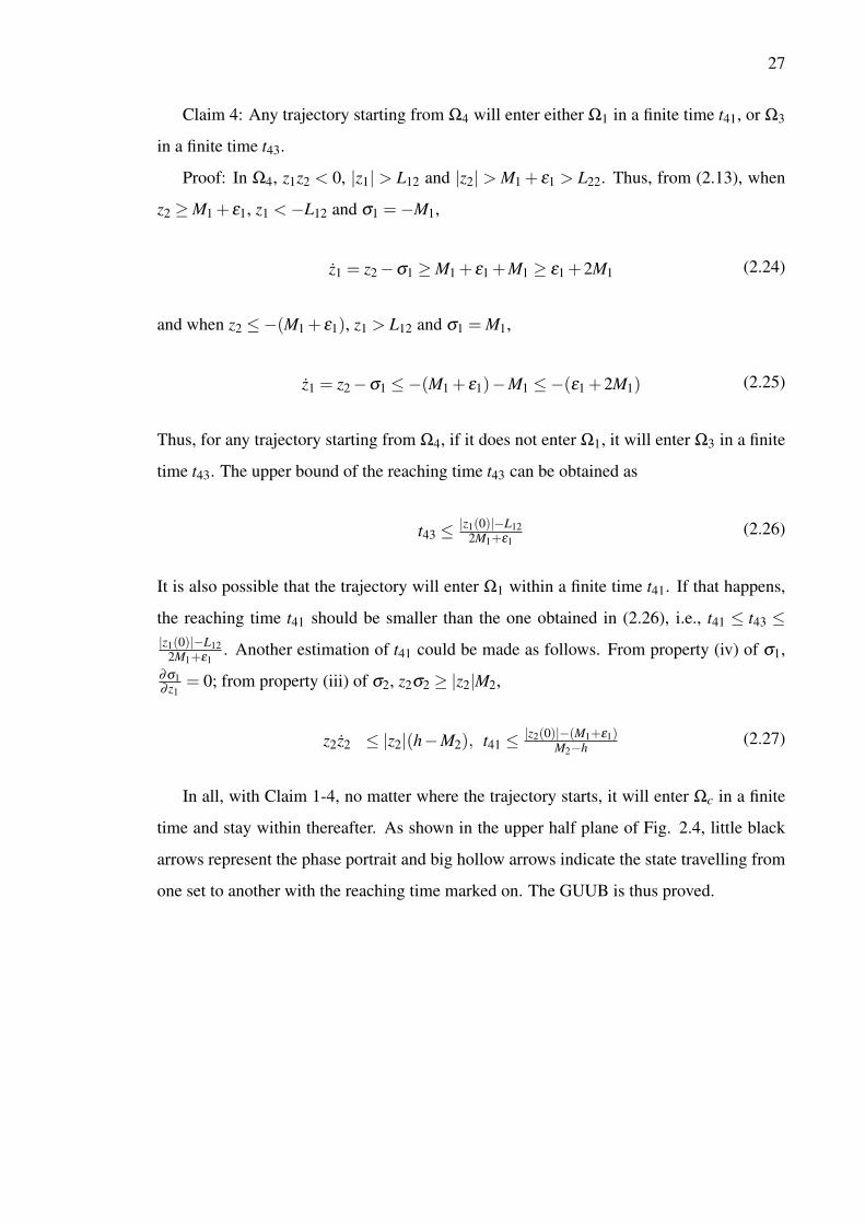
Claim 4: Any trajectory starting from Ω4 will enter either Ω1 in a finite time t41, or Ω3
in a finite time t43.
Proof: In Ω4, z1z2 < 0, |z1| > L12 and |z2| > M1 + ε1 > L22. Thus, from (2.13), when
z2 ≥M1 + ε1, z1 <−L12 and σ1 =−M1,
z1 = z2−σ1 ≥M1 + ε1 +M1 ≥ ε1 +2M1 (2.24)
and when z2 ≤−(M1 + ε1), z1 > L12 and σ1 = M1,
z1 = z2−σ1 ≤−(M1 + ε1)−M1 ≤−(ε1 +2M1) (2.25)
Thus, for any trajectory starting from Ω4, if it does not enter Ω1, it will enter Ω3 in a finite
time t43. The upper bound of the reaching time t43 can be obtained as
t43 ≤ |z1(0)|−L122M1+ε1
(2.26)
It is also possible that the trajectory will enter Ω1 within a finite time t41. If that happens,
the reaching time t41 should be smaller than the one obtained in (2.26), i.e., t41 ≤ t43 ≤|z1(0)|−L12
2M1+ε1. Another estimation of t41 could be made as follows. From property (iv) of σ1,
∂σ1∂ z1
= 0; from property (iii) of σ2, z2σ2 ≥ |z2|M2,
z2z2 ≤ |z2|(h−M2), t41 ≤ |z2(0)|−(M1+ε1)M2−h
(2.27)
In all, with Claim 1-4, no matter where the trajectory starts, it will enter Ωc in a finite
time and stay within thereafter. As shown in the upper half plane of Fig. 2.4, little black
arrows represent the phase portrait and big hollow arrows indicate the state travelling from
one set to another with the reaching time marked on. The GUUB is thus proved.

28
Once the trajectory enters Ωc = z : |z1| ≤ L11, |z2| ≤ L22, the error dynamics become,
z1 = z2− k1z1
z2 = (−ϕTb θ +∆)
+(−Bm + k1)z2−σ2(z2)
(2.28)
Define a positive semi-definite function V2 = z22/2 and let ks = k21− k1. From the second
equation of (2.28), the derivative of V2 is given by,
V2 = z2z2
≤ |z2|(h+ k1|z2|− k21|z2|)≤ − ks
2 z22 +h|z2|− ks
2 z22
≤ − ks2 (|z2|− h
ks)2 + h2
2ks− ks
2 z22
≤ h2
2ks− ks
2 z22
≤ −ksV2 + h2
2ks
(2.29)
which leads to the following inequality,
V2(t)≤ exp(−kst)V2(0)+ h2
2k2s[1− exp(−kst)] (2.30)
From (2.30), the steady state of z2 is bounded by the smaller value between hks
and L22.
Then, according to the first equation of (2.28), the steady state tracking error z1 is bounded
by the smaller value between hk1ks
and L11, as stated in Theorem 2.2.1. 4Remark 3 From this proof, it can be seen that every constraint on the control parame-
ters has its practical meaning. Constraint (a1) requires the gains in the second channel to
be greater than k1 in order to overpower the term ∂σ1∂ z1
in z2 dynamics (2.13). Constraint (b1)
guarantees that once z2 is bounded within a pre-set range, z1 is ensured to decrease and be
bounded accordingly. Constraint (c1) implies that, for the design problem to be meaning-
ful, the level of lumped modelling error and disturbance should be within the limit of the
control authority available for robust feedback. Constraint (d1) implies that a trade-off has
to be made between the amount of model uncertainties to which the system can be made

29
robust, and the aggressiveness of the trajectory that it can follow (i.e., the larger the bound
h becomes, the larger M2 is needed for robust feedback; whereas a more aggressive desired
trajectory leads to a larger bound uabd of the model compensation). Overall, these con-
straints are easy to meet practically and are favorably posed to attain the GUUB as well as
good local performance. To be more specific, theoretically, there is no absolute restriction
on how large the feedback gains (k1,k21,k22) can be. This means the steady-state tracking
error can be made arbitrarily small as seen from Theorem 1. In terms of robustness, the
controlled system can tolerate a large class of modelling error and external disturbances,
even those with a magnitude close to M2. Whereas in [53], significant conservativeness
exists in this matter.
Now that it is proved that all signals are bounded after finite time, the remainder of this
section is to demonstrate that asymptotic tracking is achievable in the presence of parameter
estimation error only, i.e., ∆ = 0.
Theorem 2.2.2 With the proposed controller (2.4)(2.12) satisfying conditions (a1)–(d1)
and the adaptation law (2.8)(2.9), asymptotic output tracking is achieved if the system
is only subject to parametric uncertainty, i.e., ∆ = 0,∀t. 4
Proof Introduce a positive semi-definite function Va = 12z2
2 + 12 θ T Γ−1θ . In the case of
∆ = 0, with property 2 of the parameter estimation law, Va becomes:
Va = z2z2 + θ T Γ−1 ˙θ
= z2(−Bmz2−ϕTb (x)θ + ∂σ1
∂ z1z2−σ2(z2))
+ θ T Γ−1Pro jθ (Γϕbz2)
≤ −Bmz22− (z2σ2(z2)− ∂σ1
∂ z1z2
2)
(2.31)
which is negative semi-definite once z1 and z2 evolve to Ωc as proved. As a result, z2
converges to zero asymptotically and so would z1 according to (2.5). Hence, asymptotic
output tracking is achieved. 4

30
2.3 Saturated Desired Compensation ARC (SDCARC)
In previous section, both the model compensation term in the control law and the pa-
rameter estimation law are calculated based on the actual states of the system. As re-
vealed in [15], certain implementation problems arose. For example, the noisy velocity
measurement may restrict the achievable performance due to the state-dependent regres-
sor. In this design, the desired trajectory replaces the actual state in the regressor for both
model compensation and parameter adaptation in order to further improve the tracking per-
formance while preserving the GUUB. Furthermore, by using the ”integration by parts”
technique [56], the resulting parameter estimation algorithm uses only the feedback posi-
tion signal, which has micrometer resolution and much less noise contamination than the
velocity signal used in SARC.
The controller design follows the same back-stepping procedure. Define z1 = x1− x1d
as the tracking error, α1 as the bounded virtual control law designed for z1 dynamics, which
is z1 = x2− x1d . Define z2 = x2−α1, then z1 dynamics become:
z1 = z2 +α1− x1d (2.32)
The adaptive robust control law for α1 is proposed as:
α1 = α1a +α1s, α1a = x1d, α1s =−σ1(z1) (2.33)
where σ1(z1) is a saturation function. Substituting (2.33) into (2.32) gives,
z1 = z2−σ1(z1) (2.34)
σ1(z1) is designed the same way as in (2.1), satisfying the same conditions as it was in
last section,with L11, L12, k1, M1 being the design parameters. Therefore, the dynamics of
z2 become:
z2 = x2− α1 = ϕT (x)θ +∆+u− x1d +∂σ1
∂ z1(z2−σ1) (2.35)

31
Let u = ua +us, where ua and us represent the model compensation and the robust term re-
spectively. Again, the essential idea is to use ua to compensate the known model dynamics
and us to deal with the model mismatch plus disturbance.
In SARC, the model compensation part is designed to be −ϕTb (x)θ plus other terms,
which needs the velocity feedback. As mentioned earlier, the experiment system is equipped
with a high resolution position encoder. The velocity signal is obtained by doing ”back-
ward difference” of the position signal, therefore certain level of noise is introduced. This
also affects the parameter adaptation since ϕTb (x) is also used there. This problems could
be solved by formulating the regressor as a function of the desired trajectory (2.36).
ua =−ϕTd θ + x1d +
∂σ1
∂ z1σ1 (2.36)
where ϕd = ϕ(xd) = [−x2d,−S f (x2d),1]T .
Given property (P1) of the parameter identifier, the known desired trajectory and prop-
erties (iii) and (iv) of σ1, it is easy to determine uabd , the upper bound of |ua|. Obviously,
for the desired trajectory to be physically trackable, uabd has to be less than the bound of
the actuator authority, i.e., |ua| ≤ uabd < ubd . As a consequence of the regressor formula-
tion, the adaptation function can be chosen as τ = ϕdz2, which is now linearly dependent
on the noise-contaminated velocity feedback. To further reduce the noise effect in imple-
mentation, the cleaner high-resolution position signal is employed instead of the velocity
feedback in the adaptation law. As a result, higher adaptation rates can be used and smaller
steady state tracking error can be achieved.
Returning to z2 dynamics (2.35) and applying the model compensation ua in (2.36)
gives,
z2 = ϕ(x)T θ −ϕTd θ +∆+ ∂σ1
∂ z1z2 +us (2.37)
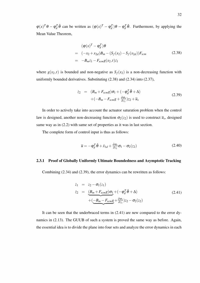
32
ϕ(x)T θ −ϕTd θ can be written as (ϕ(x)T −ϕT
d )θ −ϕTd θ . Furthermore, by applying the
Mean Value Theorem,
(ϕ(x)T −ϕTd )θ
= (−x2 + x2d)Bm− (S f (x2)−S f (x2d))Fscm
= −Bmz1−Fscmg(x2, t)z1
(2.38)
where g(x2, t) is bounded and non-negative as S f (x2) is a non-decreasing function with
uniformly bounded derivatives. Substituting (2.38) and (2.34) into (2.37),
z2 = (Bm +Fscmg)σ1 +(−ϕTd θ +∆)
+(−Bm−Fscmg+ ∂σ1∂ z1
)z2 +us
(2.39)
In order to actively take into account the actuator saturation problem when the control
law is designed, another non-decreasing function σ2(z2) is used to construct us, designed
same way as in (2.2) with same set of properties as it was in last section.
The complete form of control input is thus as follows:
u =−ϕTd θ + x1d + ∂σ1
∂ z1σ1−σ2(z2) (2.40)
2.3.1 Proof of Globally Uniformly Ultimate Boundedness and Asymptotic Tracking
Combining (2.34) and (2.39), the error dynamics can be rewritten as follows:
z1 = z2−σ1(z1)
z2 = (Bm +Fscmg)σ1︸ ︷︷ ︸+(−ϕTd θ +∆)
+(−Bm−Fscmg︸ ︷︷ ︸+∂σ1∂ z1
)z2−σ2(z2)
(2.41)
It can be seen that the underbraced terms in (2.41) are new compared to the error dy-
namics in (2.13). The GUUB of such a system is proved the same way as before. Again,
the essential idea is to divide the plane into four sets and analyze the error dynamics in each

33
one. The conclusion is that no matter where the initial state starts, the trajectory will reach
the invariant set Ωc = z1,z2 : |z1| ≤ L11, |z2| ≤ L22 in finite time with the upper bound of
the reaching time estimated accordingly.
As to the additional terms, (Bm + Fscmg)σ1 can be lumped with the model mismatch
−ϕTd θ +∆ and the total effect can be found bounded by a constant h, i.e., |(Bm +Fscmg)σ1−
ϕTd θ +∆)| ≤ h, since all the signals involved are bounded. Furthermore, (−Bm−Fscmg)z2
actually acts as a damping term, which helps to preserve stability even though its effect is
trivial compared to the high gain robust term.
To prove the GUUB of the controlled system, the following constraints are required
for design parameters: (a2) k21 > k1, (b2) k1L11 > L22, (c2) h < M2− k1M1, and (d2) M2 ≤ubd−uabd . They are exactly the same as conditions (a1)–(d1) except that h, the upper bound
of the lumped uncertainties, might be slightly increased here.
Theorem 2.3.1 With the proposed controller (2.33)(2.40) satisfying conditions (a2)–(d2),
all signals are bounded. Furthermore, the error state [z1,z2]T reaches the invariant set Ωc
in a finite time and stay within thereafter. At steady state, the final tracking error is bounded
above as |z1(∞)| ≤min hk1(k21−k1)
,L11. 4
The proof of if Theorem 2.3.1 is the same as of Theorem 2.2.1.
If the considered system is subject to parametric uncertainties only, better performance
such as zero final tracking error can be achieved. To prove the asymptotic tracking, a
strengthened constraint denoted as (a∗2) is posed along with constraints (b2)-(d2):
(a∗2) k21− k1 > 12(Bm +Fscmg+1)2
Theorem 2.3.2 With the proposed controller (2.33)(2.40) satisfying conditions (a∗2),(b2)–
(d2) and the adaptation law (5.18)(5.19), asymptotic output tracking is achieved if the
system is only subject to parametric uncertainty, i.e., ∆ = 0,∀t. 4
Proof Following Theorem 2.3.1, the trajectory will eventually enter Ωc = z : |z1| ≤L11, |z2| ≤ L22, then the asymptotic tracking under condition ∆ = 0 is proved as follows.
34
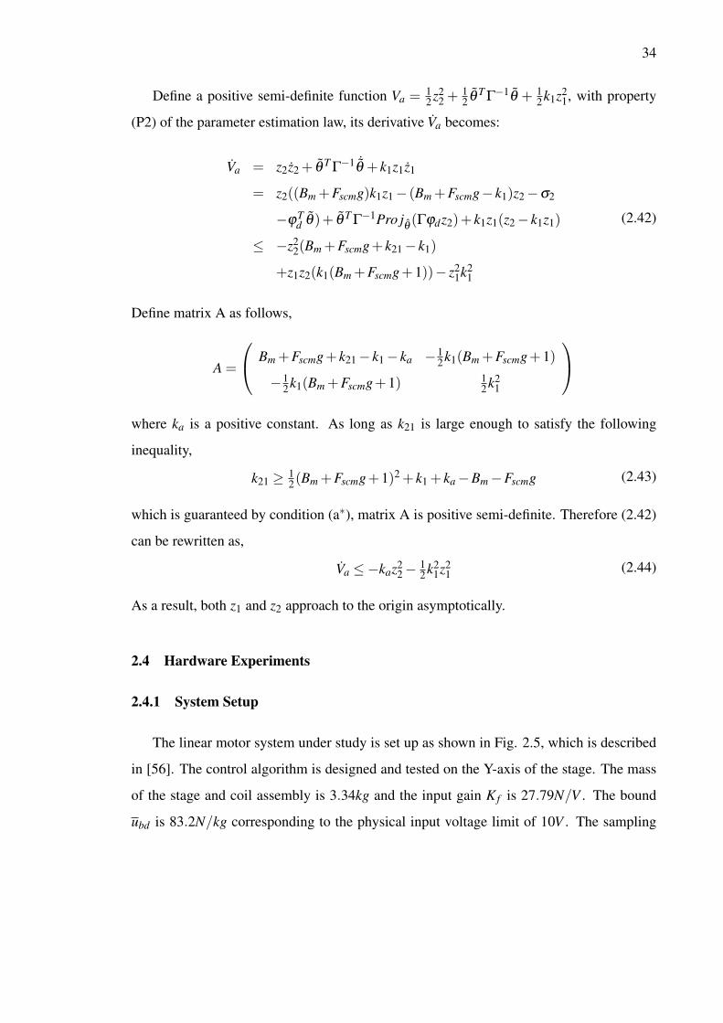
Define a positive semi-definite function Va = 12z2
2 + 12 θ T Γ−1θ + 1
2k1z21, with property
(P2) of the parameter estimation law, its derivative Va becomes:
Va = z2z2 + θ T Γ−1 ˙θ + k1z1z1
= z2((Bm +Fscmg)k1z1− (Bm +Fscmg− k1)z2−σ2
−ϕTd θ)+ θ T Γ−1Pro jθ (Γϕdz2)+ k1z1(z2− k1z1)
≤ −z22(Bm +Fscmg+ k21− k1)
+z1z2(k1(Bm +Fscmg+1))− z21k2
1
(2.42)
Define matrix A as follows,
A =
Bm +Fscmg+ k21− k1− ka −1
2k1(Bm +Fscmg+1)
−12k1(Bm +Fscmg+1) 1
2k21
where ka is a positive constant. As long as k21 is large enough to satisfy the following
inequality,
k21 ≥ 12(Bm +Fscmg+1)2 + k1 + ka−Bm−Fscmg (2.43)
which is guaranteed by condition (a∗), matrix A is positive semi-definite. Therefore (2.42)
can be rewritten as,
Va ≤−kaz22− 1
2k21z2
1 (2.44)
As a result, both z1 and z2 approach to the origin asymptotically.
2.4 Hardware Experiments
2.4.1 System Setup
The linear motor system under study is set up as shown in Fig. 2.5, which is described
in [56]. The control algorithm is designed and tested on the Y-axis of the stage. The mass
of the stage and coil assembly is 3.34kg and the input gain K f is 27.79N/V . The bound
ubd is 83.2N/kg corresponding to the physical input voltage limit of 10V . The sampling

35
frequency is 2.5kHz. The resolution of the position sensor is 1µm and the feedback velocity
signal is obtained by conducting ”back difference” of the position feedback.
Figure 2.5. Experiment setup of linear motor system.
2.4.2 Implementation Issue and Design Parameters with SARC
When implementing the designed control law in real-time experiments, a modification
on function σ2 is used to further improve the performance. The example σ2 as shown in
Fig. 2.2 has a constant control effort as |z2| > L22, which introduces a certain degree of
conservativeness. In other words, the actual amount of control effort for the model com-
pensation ua during most of the running period is much smaller than the estimated upper
bound. Therefore the actuator has not put in all available power to attenuate the disturbance
although the robust control term reaches its maximum value. To improve the system’s abil-
ity to cope with large disturbances, the magnitude restriction on function σ2 is removed so
that σ2 keeps increasing monotonically and the physical actuator becomes saturated natu-
rally. Such a σ2 still satisfies properties (i) to (iii) and thus the overall system’s GUUB is
guaranteed.

36
The control parameters are selected as follows, L11 = 50µm, L12 = 70µm, k1 = 500,
M1 = 1.2k1L11, L21 = 0.5M1, k21 = k1 + 600, k22 = k21 + 200, M2 = 0.99(ubd − uabd),
L22 = (M22− k21L21)/k22 +L21.
2.4.3 Implementation Issue and Design Parameters with SDCARC
As mentioned in the Controller Structure section, there are two main issues which need
further consideration in implementation.
The motor system is normally equipped with a high-resolution encoder which provides
very clean position feedback in contrast to a noisy velocity signal. To further alleviate the
noise effect, the parameter estimates can be updated as follows [56]. Let i represent the
sampling instant, T represent the sampling period, θ j be the j-th parameter to be estimated,
ϕd, j and γ j be the corresponding desired regressor and adaptation rate. Then the digital
implementation of the adaptation law under the normal condition, i.e. when θ stays within
the bound, is
θ j((i+1)T ) = θ j(iT )+ γ j
∫ (i+1)T
iTϕd, jz2dt
= θ j(iT )+ γ j
∫ (i+1)T
iTϕd, j(z1 +σ1)dt
= θ j(iT )+ γ j(∫ (i+1)T
iTϕd, jσ1dt
+[ϕd, jz1](i+1)TiT −
∫ (i+1)T
iT˙ϕd, jz1dt)
(2.45)
Thus the parameter adaptation law implemented by (2.45) is free of velocity measurement
noise.
Another modification is made to function σ2 the same way as in last subsection.
Design parameters are determined from conditions (a2)–(d2) described before. Further-
more, with a clean position signal employed in the parameter adaptation law, higher robust
gain and adaptation rates can be utilized for this scheme.

37
The control parameters are selected as follows, L11 = 25µm, L12 = 30µm, k1 = 750,
M1 = 0.0206, L21 = 0.0094m, k21 = k1 + 600, k22 = k21 + 200, M2 = 0.99(ubd − uabd),
L22 = (M2− k21L21)/k22 +L21.
2.4.4 Real-time Experimental Results with SARC
Two sets of desired trajectories are designed to illustrate the effectiveness of the pro-
posed control law. The point-to-point trajectory duplicates the regular maneuver in the
manufacturing industry, while the step trajectory represents the extreme case for the linear
motor to track.
Point-To-Point Trajectory
The point-to-point trajectory is at least second order differentiable (meaning the accel-
eration being continuous), with a distance of 0.4m, a maximum velocity of 1m/s and a
maximum acceleration of 12m/s2 as shown in Fig. 2.6 [56].
The experimental results with the proposed saturated ARC are given in Fig. 2.7 and
Fig. 2.8. It can be seen that the position error converges quickly in Fig. 2.7 and the
steady state error is within 1µm. Both transient and steady state performances could be
improved by employing a better parameter estimation algorithm such as recursive least
squares method [8].
Fig. 2.8 shows the tracking error and control effort under a 1V constant disturbance
added to the physical control input u. It is about ten percents of the total control authority,
which represents the normal working environment. With Simulink program, the distur-
bance is introduced to the system at 3 second and lasts 10 seconds. As can be seen from
the plot, the system adjusts well and the tracking error remains at the same level as it is
in Fig. 2.7 due to the parameter adaptation mechanism. The parameter estimates are not
shown here because the estimation law used here can not guarantee the convergence of the
estimate error.
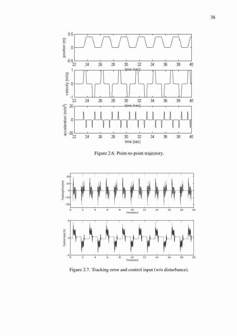
38
Figure 2.6. Point-to-point trajectory.
0 2 4 6 8 10 12 14 16 18 20
−20
−10
0
10
20
Time(sec)
Trac
king
Erro
r(um
)
0 2 4 6 8 10 12 14 16 18 20−5
0
5
Time(sec)
Con
trol I
nput
(V)
Figure 2.7. Tracking error and control input (w/o disturbance).

39
0 2 4 6 8 10 12 14 16 18 20
−20
−10
0
10
20
Time(sec)
Trac
king
Erro
r(um
)
0 2 4 6 8 10 12 14 16 18 20−6
−4
−2
0
2
4
Time(sec)
Con
trol I
nput
(V)
Figure 2.8. Tracking error and control input (w/1V disturbance).

40
To demonstrate the GUUB of the proposed saturated controller, as well as how effec-
tively the controlled system deals with the practical scenario of experiencing an accident,
such as a strong but short disturbance, experiments are conducted as follows. The actual
input limit of the hardware is 10V , while the physical limit of the control input is purposely
set at 4V , so that a step input, with the amplitude of 6V and a duration of 0.1 second, can be
injected as a disturbance and implemented by the hardware. The desired trajectory is also
changed to be less aggressive due to the reduced control input authority, with a distance of
0.1m, a maximum velocity of 0.02m/s and a maximum acceleration of 0.1m/s2.
Experimental results are shown in Fig. 2.9 through Fig. 2.11. Fig. 2.9 provides an
overall view of the tracking error and control input during the entire operation time. Fig.
2.10 emphasizes on the time period when the strong input disturbance happens. As seen
from the plots, when the strong input disturbance is inserted at 3 second, the control input
is not sufficient to overpower the disturbance and it saturates at the 4V limit level with the
tracking error accumulating to over 0.05m. After the strong input disturbance is removed
0.1 second later, the tracking error reduces to the encoder resolution level of 1µm at steady
state as shown in Fig. 2.11.
The above results support the claim that the proposed saturated ARC can achieve high
performance under normal working environment and ensure GUUB in case of unexpected
strong disturbances.
Step Trajectory
Normally, step signal is not a feasible trajectory for a physical system to track due to
the infinite value of its derivative at the step instant. The system will have large initial error
which would easily saturate the control input with high gain feedback and cause potential
instability. Therefore, certain trajectory planning between the initial point and the set point
is necessary to avoid that problem. The point-to-point trajectory described in the above
section is an example of a feasible one. However, in a few industry applications such
as the hard disk drive (HDD) servomechanism, point-to-point movement is frequent and

41
0 2 4 6 8 10 12 14 16 18 20−0.01
0
0.01
0.02
0.03
0.04
0.05
0.06
Time(sec)
Trac
king
Erro
r(m)
0 2 4 6 8 10 12 14 16 18 20
−4
−3
−2
−1
0
1
Time(sec)
Con
trol I
nput
(V)
Figure 2.9. Tracking error and control input (w/6V disturbance).
2.5 3 3.5 4 4.5 5 5.5−0.01
0
0.01
0.02
0.03
0.04
0.05
0.06
Time(sec)
Trac
king
Erro
r(m)
2.5 3 3.5 4 4.5 5 5.5
−4
−3
−2
−1
0
1
Time(sec)
Con
trol I
nput
(V)
Figure 2.10. Tracking error and control input (in the presence of 6V disturbance).

42
6 7 8 9 10 11 12−4
−2
0
2
4
6
Time(sec)
Trac
king
Erro
r(um
)
6 7 8 9 10 11 12−2
−1.5
−1
−0.5
0
0.5
1
Time(sec)
Con
trol I
nput
(V)
Figure 2.11. Tracking error and control input (zoomed in portion at s.s).
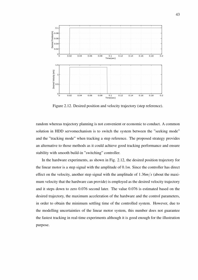
43
0 0.02 0.04 0.06 0.08 0.1 0.12 0.14 0.16 0.18 0.20
0.02
0.04
0.06
0.08
0.1
Time(sec)
Des
ired
Posi
tion(
m)
0 0.02 0.04 0.06 0.08 0.1 0.12 0.14 0.16 0.18 0.20
0.5
1
1.5
Time(sec)
Des
ired
Velo
city
(m/s
)
Figure 2.12. Desired position and velocity trajectory (step reference).
random whereas trajectory planning is not convenient or economic to conduct. A common
solution in HDD servomechanism is to switch the system between the ”seeking mode”
and the ”tracking mode” when tracking a step reference. The proposed strategy provides
an alternative to those methods as it could achieve good tracking performance and ensure
stability with smooth build-in ”switching” controller.
In the hardware experiments, as shown in Fig. 2.12, the desired position trajectory for
the linear motor is a step signal with the amplitude of 0.1m. Since the controller has direct
effect on the velocity, another step signal with the amplitude of 1.36m/s (about the maxi-
mum velocity that the hardware can provide) is employed as the desired velocity trajectory
and it steps down to zero 0.076 second later. The value 0.076 is estimated based on the
desired trajectory, the maximum acceleration of the hardware and the control parameters,
in order to obtain the minimum settling time of the controlled system. However, due to
the modelling uncertainties of the linear motor system, this number does not guarantee
the fastest tracking in real-time experiments although it is good enough for the illustration
purpose.

44
0 0.02 0.04 0.06 0.08 0.1 0.12 0.14 0.16 0.18 0.2
−0.1
−0.08
−0.06
−0.04
−0.02
0
Time(sec)
Trac
king
Erro
r(m)
0 0.02 0.04 0.06 0.08 0.1 0.12 0.14 0.16 0.18 0.2
−10
−5
0
5
10
Time(sec)
Con
trol I
nput
(V)
Figure 2.13. Tracking error and control input (step reference).
The experimental results with the step references are shown in Fig. 2.13 the overall
response, and Fig. 2.14 the zoomed in portion at its steady state. As can be seen on
Fig. 2.13, the actuator uses its maximum power ±10V to speed up at the beginning and
slow down when the stage is close to the 0.1m set point. Between the acceleration and
deceleration, the stage approaches to the set point at full speed. With this strategy, the
controlled system can track the step reference with minimum time. Fig. 2.14 shows that
the final tracking error is at the 1µm resolution level and it enters the range of ±10µm,
0.01percent of the travel distance, after approximately 0.12 second.
2.4.5 Comparative Experimental Results with SDCARC, SARC and PID
The desired trajectory is the point-to-point movement, same as previous section, with a
distance of 0.4m, a maximum velocity of 1m/s and a maximum acceleration of 12m/s2.
The comparative experiments are conducted with three controllers under two different
conditions, with no disturbances and with 1V input disturbance respectively. The con-
trollers are: (i) the conventional PID with similar closed-loop bandwidth [56], (ii) the sat-

45
0.14 0.15 0.16 0.17 0.18 0.19 0.2
−8
−6
−4
−2
0
Time(sec)
Trac
king
Erro
r(um
)
0.14 0.15 0.16 0.17 0.18 0.19 0.2−0.2
−0.1
0
0.1
0.2
0.3
0.4
0.5
Time(sec)
Con
trol I
nput
(V)
Figure 2.14. Tracking error and control input at s.s.(step reference).

46
urated ARC (SARC) described in section 2.2, and (iii) the saturated DCARC (SDCARC)
proposed in section 2.3. The tracking errors with three controllers under different condi-
tions are compared in Fig. 2.15 and Fig. 2.18. Fig. 2.16 and Fig. 2.19 are the magnified
views over one moving period. The control inputs are shown in Fig. 2.17 and Fig. 2.20.
Under both conditions, it is seen that the proposed SDCARC achieves the best position
tracking performance. In order to gain more insight in a quantitative manner, the perfor-
mance indexes used in [56] are listed in Table 2.1 to make the comparison more apparent.
The meanings of all the indexes are briefly described as follows. eM is the maximum
tracking error of the entire running time; eF is the maximum tracking error of the last two
seconds, which represents the steady state error; L2[e] represents the energy of the tracking
error; L2[u] represents the energy of the control input; Cu shows the chattering level of the
control input. These results verify the high-performance nature of the proposed SDCARC,
and the performance robustness to disturbances and modeling uncertainties under normal
working conditions.
Table 2.1 Performance indexes of three controllers.
w/o disturbance w/ disturbancecontroller PID SARC SDCARC PID SARC SDCARCeM (µm) 23.1 27.6 11.1 33.0 31.0 15.2eF (µm) 22.5 26.8 10.4 23.0 26.7 11.4
L2[e] (µm) 3.89 5.06 1.82 4.57 5.18 2.45L2[u] (V ) 1.02 1.09 1.02 1.41 1.34 1.26
Cu 0.191 0.146 0.352 0.138 0.118 0.285
To illustrate the GUUB of the proposed SDCARC, as well as how effectively the con-
trolled system deals with the practical scenario of experiencing an accident, such as a strong
but short disturbance, experiments are conducted as follows. The actual input limit of the
hardware is 10V, therefore the physical limit of the control input is purposely set at 4V , so
that a step input, with the amplitude of 6V and a duration of 0.1 second, can be injected as a
disturbance and realized by the hardware. The desired trajectory is also changed to be less
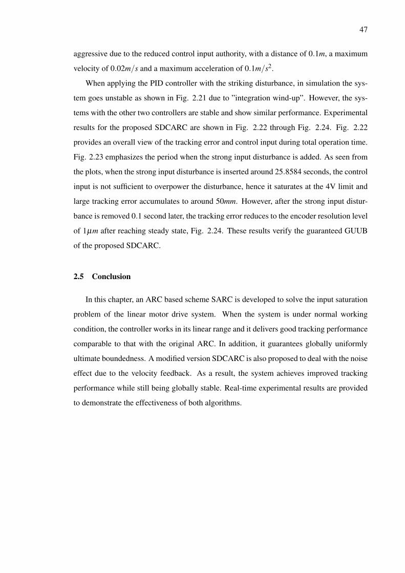
47
aggressive due to the reduced control input authority, with a distance of 0.1m, a maximum
velocity of 0.02m/s and a maximum acceleration of 0.1m/s2.
When applying the PID controller with the striking disturbance, in simulation the sys-
tem goes unstable as shown in Fig. 2.21 due to ”integration wind-up”. However, the sys-
tems with the other two controllers are stable and show similar performance. Experimental
results for the proposed SDCARC are shown in Fig. 2.22 through Fig. 2.24. Fig. 2.22
provides an overall view of the tracking error and control input during total operation time.
Fig. 2.23 emphasizes the period when the strong input disturbance is added. As seen from
the plots, when the strong input disturbance is inserted around 25.8584 seconds, the control
input is not sufficient to overpower the disturbance, hence it saturates at the 4V limit and
large tracking error accumulates to around 50mm. However, after the strong input distur-
bance is removed 0.1 second later, the tracking error reduces to the encoder resolution level
of 1µm after reaching steady state, Fig. 2.24. These results verify the guaranteed GUUB
of the proposed SDCARC.
2.5 Conclusion
In this chapter, an ARC based scheme SARC is developed to solve the input saturation
problem of the linear motor drive system. When the system is under normal working
condition, the controller works in its linear range and it delivers good tracking performance
comparable to that with the original ARC. In addition, it guarantees globally uniformly
ultimate boundedness. A modified version SDCARC is also proposed to deal with the noise
effect due to the velocity feedback. As a result, the system achieves improved tracking
performance while still being globally stable. Real-time experimental results are provided
to demonstrate the effectiveness of both algorithms.
48
24 26 28 30 32 34 36 38 40
−20
0
20
time (sec)
po
sitio
n e
rro
r(u
m)
24 26 28 30 32 34 36 38 40
−20
0
20
time (sec)
po
sitio
n e
rro
r(u
m)
24 26 28 30 32 34 36 38 40
−20
0
20
time (sec)
po
sitio
n e
rro
r(u
m)
PID
SARC
SDCARC
Figure 2.15. Tracking error with no disturbance.

49
31 31.1 31.2 31.3 31.4 31.5 31.6 31.7 31.8 31.9 32
−20
0
20
time (sec)
po
sitio
n e
rro
r(u
m)
30.8 30.9 31 31.1 31.2 31.3 31.4 31.5 31.6 31.7 31.8
−20
0
20
time (sec)
po
sitio
n e
rro
r(u
m)
29.8 29.9 30 30.1 30.2 30.3 30.4 30.5 30.6 30.7 30.8
−20
0
20
time (sec)
po
sitio
n e
rro
r(u
m)
PID
SARC
SDCARC
Figure 2.16. Tracking error with no disturbance (zoomed in portion).

50
24 26 28 30 32 34 36 38 40−5
0
5
time (sec)
con
tro
l in
pu
t (V
)
24 26 28 30 32 34 36 38 40−5
0
5
time (sec)
con
tro
l in
pu
t (V
)
24 26 28 30 32 34 36 38 40−5
0
5
time (sec)
con
tro
l in
pu
t (V
)
PID
SARC
SDCARC
Figure 2.17. Control input with no disturbance.

51
22 24 26 28 30 32 34 36 38
−20
0
20
time (sec)
po
sitio
n e
rro
r(u
m)
24 26 28 30 32 34 36 38 40
−20
0
20
time (sec)
po
sitio
n e
rro
r(u
m)
24 26 28 30 32 34 36 38 40
−20
0
20
time (sec)
po
sitio
n e
rro
r(u
m)
PID
SARC
SDCARC
Figure 2.18. Tracking error with 1V disturbance.

52
30.5 30.6 30.7 30.8 30.9 31 31.1 31.2 31.3 31.4 31.5
−20
0
20
time (sec)
po
sitio
n e
rro
r(u
m)
30.8 30.9 31 31.1 31.2 31.3 31.4 31.5 31.6 31.7 31.8
−20
0
20
time (sec)
po
sitio
n e
rro
r(u
m)
29.8 29.9 30 30.1 30.2 30.3 30.4 30.5 30.6 30.7 30.8
−20
0
20
time (sec)
po
sitio
n e
rro
r(u
m)
PID
SARC
SDCARC
Figure 2.19. Tracking error with 1V disturbance (zoomed in portion).

53
22 24 26 28 30 32 34 36 38−6
−4
−2
0
2
4
time (sec)
con
tro
l in
pu
t (V
)
24 26 28 30 32 34 36 38 40−6
−4
−2
0
2
4
time (sec)
con
tro
l in
pu
t (V
)
24 26 28 30 32 34 36 38 40−6
−4
−2
0
2
4
time (sec)
con
tro
l in
pu
t (V
)
PID
SARC
SDCARC
Figure 2.20. Control input with 1V disturbance.
20 25 30 35 40 45 50−3
−2
−1
0
1
2
3
time (sec)
posi
tion
erro
r(m)
20 25 30 35 40 45 50−4
−2
0
2
4
time (sec)
cont
rol i
nput
(V)
Figure 2.21. PID with 6V disturbance.

54
20 25 30 35 40 45 50−0.01
0
0.01
0.02
0.03
0.04
0.05
0.06
time (sec)
posi
tion
erro
r(m)
20 25 30 35 40 45 50−4
−2
0
2
4
time (sec)
cont
rol i
nput
(v)
Figure 2.22. SDCARC with 6V disturbance (the whole process).
25.5 26 26.5 27 27.5 28 28.5 29−0.01
0
0.01
0.02
0.03
0.04
0.05
0.06
time (sec)
posi
tion
erro
r(m)
25.5 26 26.5 27 27.5 28 28.5 29
−4
−2
0
2
4
time (sec)
cont
rol i
nput
(v)
Figure 2.23. SDCARC with 6V disturbance (in the presence of the disturbance).

55
35 36 37 38 39 40 41−6
−4
−2
0
2
4
time (sec)
posi
tion
erro
r(um
)
35 36 37 38 39 40 41−1
−0.5
0
0.5
1
1.5
2
time(sec)
cont
rol i
nput
(v)
Figure 2.24. SDCARC with 6V disturbance (zoomed in portion at stead-state).

56
3. SATURATED ADAPTIVE ROBUST CONTROL WITH UNKNOWN MASS
In previous chapter, the mass of the moving stage plus load is assumed given. Its value
can be either calculated via manufacture data or estimated via offline system identification.
Based on this knowledge and the given saturation level of the actuator, the control parame-
ters of the proposed SARC or SDCARC are then designed to achieve the best performance
allowed by the hardware system. However, this assumption is not practical for most in-
dustrial applications. It is more desirable to have a controlled system which is able to
accommodate load variation to certain extend rather that one which needs to have the load
weighed and design parameters adjusted accordingly every time a new object is mounted
to the moving stage. In this chapter, the original saturation adaptive robust control law is
modified to deal with parameter uncertainty including the mass variation.
The essential idea of the SARC with unknown mass is to use different sets of control
parameters before and after online estimation law identifies the unknown mass. Before the
mass is estimated, the control parameters are designed to satisfy a relatively conservative set
of constraints in order to guarantee globally uniformly ultimate boundedness (GUUB) of
the overall system. Once the mass gets identified with reasonable accuracy, the constraints
will be relaxed and the design parameters will be online recalculated to achieve better
performance. The key to the success of this strategy is to estimate the unknown mass
quickly and accurately.
Again, the linear motor drive system is used as a case of study. The control input
to the motor has an amplitude saturation limit. In spite of the load variation, an ARC-
based control law is synthesized to deal with the input saturation problem. The closed-loop
system is guaranteed globally uniformly ultimately bounded all the time and the tracking
performance is improved once the parameter estimation law identifies the unknown mass.
Real-time experiments are carried out and the results validate the above claims.

57
3.1 Problem Formulation and Practical Assumptions
Revisit the equation of motion of the linear motor positioning system as in Chapter 2
equation (2.1), one gets:
x1 = x2
mx2 = −Bx2−FscS f (x2)+d(t)+K f u
= ϕT (x)θ +∆+u
(3.1)
where m is the mass of the payload plus the coil assembly, u is the control voltage with an
input gain of K f which can be calculated from manufacture data, B and Fsc represent two
major friction coefficients, viscous and Coulomb respectively, S f (x2) is a non-decreasing
continuous function that approximates the mode of Coulomb friction, and d(t) represents
the lumped external disturbances and modelling uncertainty. In the second line of the
second equation, the expression is rewritten with ϕ(x) = [−x2,−S f (x2),1]T as the regres-
sor, θ = [B,Fsc,d0]T and the mass m are the unknown parameters to be estimated online,
∆ = d(t)−d0 represents the high frequency components of d(t), and u = K f u is the control
effort amplified by the input gain and its bound ubd as in |u(t)| ≤ ubd can be calculated in
advance.
All the motor parameters (m, B, Fsc and d0) are unknown, but the extents of the uncer-
tainty can be determined in advance, and the mass m keeps constant during one controlled
maneuver. Also, the lumped modelling errors and external disturbance is bounded. The
formal way of putting these assumptions is as follows,
Assumption 1:
m ∈ [ml,mu],B ∈ [Bl,Bu],Fsc ∈ [Fscl,Fscu]
where ml , mu, Bl , Bu, Fscl , Fscu are the lower bounds and upper bounds which are deter-
mined in advance, and m is an unknown constant.
Assumption 2: The lumped uncertainty d(t) is bounded, i.e.,
|d(t)| ≤ δd

58
where δd is a known constant.
The design objective is, under above two assumptions and the control input constraint
|u(t)| ≤ ubd , to synthesize an ARC-based control law which can globally stabilize the plant
(3.1) and achieve good tracking/regulating performance under nominal working condition.
As stated in the previous chapter, the desired trajectory (position x1d(t), velocity x2d(t) =
x1d(t) and acceleration x1d(t)) for the tracking control is bounded and smooth up to the
second order. Rather than offline calculated in the previous case, it could be updated online
based on the identified mass to push performance to the limit.
3.2 Controller Design
According to the standard back-stepping design procedure [8], the difference between
the actual position and the desired position z1 = x1− x1d is defined as the output tracking
error. α1 is the bounded virtual control law designed for z1 dynamics, which is z1 = x2− x1d .
Define z2 = x2−α1, then z1 dynamics become:
z1 = z2 +α1− x1d (3.2)
The saturation control design for the first channel input α1 is the same as it is done in
previous chapter:
α1 = α1a +α1s, α1a = x1d, α1s =−σ1(z1) (3.3)
where σ1(z1) is a smooth saturation function described in Fig. 2.1, with design parameters
L11, L12, k1, M1. Again, the logic of this design is to achieve local high-gain and ensure
global boundedness as well so that when it propagates to the second channel which in this
case is also the last channel involving the actual control input, all signals would remain
bounded within the scope of the input power.

59
Substituting (3.3) into (3.2) gives,
z1 = z2−σ1(z1) (3.4)
Now the objective is to drive z2 to zero or a pre-set small bound so that z1 will converge to
zero or small value. From (3.1), (3.3) and (3.4), the equation of z2 becomes:
mz2 = mx2−mα1 = ϕT (x)θ +∆+u−mx1d +m∂σ1
∂ z1(z2−σ1) (3.5)
At this stage, one might attempt to divide mass m from both sides of (3.5) to make it
in the standard form to apply the back-stepping design. However, dividing the unknown
mass from other unknown parameters results in larger range of parameter uncertainty and
requires more control power to cover, this could make the design a little more conservative.
Let u = ua +us, where ua and us represent the model compensation and the robust term
respectively. For the model compensation part, parameter estimate θ is obtained online to
take the place of the true value θ . Inspired by the integrated direct/indirect ARC proposed
in [17], least squares type of adaptation law is employed to estimate unknown parameters
m and θ since (a) it guarantees the boundedness of the parameter estimates as Property
(P1) in last chapter; (b) the least squares estimation law has better convergence property.
And a gradient type adaptation law is employed to estimate a constant dl acting as an
integral compensation to achieve zero steady state error. Different treatment is brought to
the compensation terms related to unknown mass m due to the important role it plays on the
matter of system stability. At the beginning, a standard recursive least squares algorithm is
applied to provide m and θ as the estimates of m and θ . At the same time, a batch least
squares algorithm also keeps collecting data to get a quicker and more accurate estimate
of the unknown mass, denoted as m∗. Once m∗ is obtained, the control law updates its
parameters according to this estimate to achieve better tracking performance. The control
law at the beginning is as follows:
ua =−ϕTb θ − dl + mx1d + m
∂σ1
∂ z1σ1 (3.6)

60
where ϕb = [−α1,−S f (x2),1]T is the regressor guaranteed to be bounded, m and θ are the
parameter estimates, and dl is the estimate of dl for direct compensation. Since all the terms
on the right hand side of equation (3.6) have known bounds, the bound of ua, uabd can be
calculated, which enables us to determine the bound of the robust term.
The robust term, us =−σ2(z2) is designed as shown in Fig. 2.2, with L21, k21, L22, k22
being design parameters to be determined later. Again, such design of σ2(z2) provides a
local high-gain feedback when error is fairly small under normal working condition, a little
more aggressive feedback gain when system is enduring large transient error either due to
parameter uncertainty or because of bad initial condition, and constantly maximum power
when error is abnormally large due to overpowering external disturbance or extremely ag-
gressive desired trajectory.
Combine (3.6) and the design for us, one gets the complete expression of the control
law u as:
u =−ϕTb θ − dl + mx1d + m
∂σ1
∂ z1σ1−σ2(z2) (3.7)
Plugging (3.7) back into z2 dynamics (3.5) gives:
mz2 = ϕT θ −ϕTb θ − dl +∆+ mx1d + m∂σ1
∂ z1σ1 +m∂σ1
∂ z1z2−σ2
= −ϕTb θ − dl +∆+ mx1d + m∂σ1
∂ z1σ1
+ (−B+m∂σ1∂ z1
)z2−σ2
(3.8)
where m = m−m, θ = θ −θ , dl = dl −dl . Based on the two practical assumptions made
on the plant, the property of boundedness on the parameter estimates, and the saturated
controller design, a positive constant h can be found to represent the bound of the total
amount of uncertainties as follows:
|−ϕTb θ − dl +∆+ mx1d + m
∂σ1
∂ z1σ1| ≤ h.

61
Then the error dynamics could be simplified as
z1 = z2−σ1
mz2 ≤ h−Bz2 +m∂σ1∂ z1
z2−σ2
(3.9)
3.3 Proof of Globally Uniformly Ultimate Boundedness
Following the same idea of the original stability proof, one can get the same result
if the following conditions on the control parameters are satisfied: (a3) k21 > k1mu, (b3)
k1L11 > L22, (c3) h < M2−k1M1mu, and (d3) M2 ≤ ubd−uabd . Comparing these conditions
to the original constraints (a1)-(d1) in Chapter 2, one can see that the only difference is
that the upper bound of varying mass mu shows up in two of these conditions, which is
very reasonable considering both the control law u and the uncertainty bound h here are
approximately the products of the mass and their counterparts in the original design. Since
the accurate estimate of the unknown mass is unavailable at this stage, putting the upper
bound mu in the design constraints guarantees the GUUB even for the worst case scenario.
Theorem 3.3.1 With any parameter adaptation law that guarantees boundedness on the
estimates, and the proposed controller (3.3)(3.7) satisfying conditions (a3)–(d3), all signals
are bounded. Furthermore, the error state [z1,z2]T reaches the invariant set Ωc = z : |z1| ≤L11, |z2| ≤ L22 in a finite time and stay within thereafter. At steady state, the final tracking
error is bounded above by |z1(∞)| ≤min hk1(k21−k1mu)
,L11. 4
Proof: First define the invariant set Ωc = z : |z1| ≤ L11, |z2| ≤ L22. Because of condi-
tions (b3) and (c3), there exist positive ε1,ε2 and ε3, such that h+k1mu(M1 +ε1)+ε2 < M2
and L22 + ε3 < k1L11. Notice that M1 > k1L11 > L22, as shown in Fig. 2.5, the entire z1-z2
plane is divided into four sets Ω1-Ω4 defined as follows.
Ω1 = z : |z2| ≤M1 + ε1Ω2 = z : z2(z1− sign(z2)L12) > 0, |z2|> M1 + ε1Ω3 = z : |z1| ≤ L12, |z2|> M1 + ε1Ω4 = z : z2(z1 + sign(z2)L12) < 0, |z2|> M1 + ε1
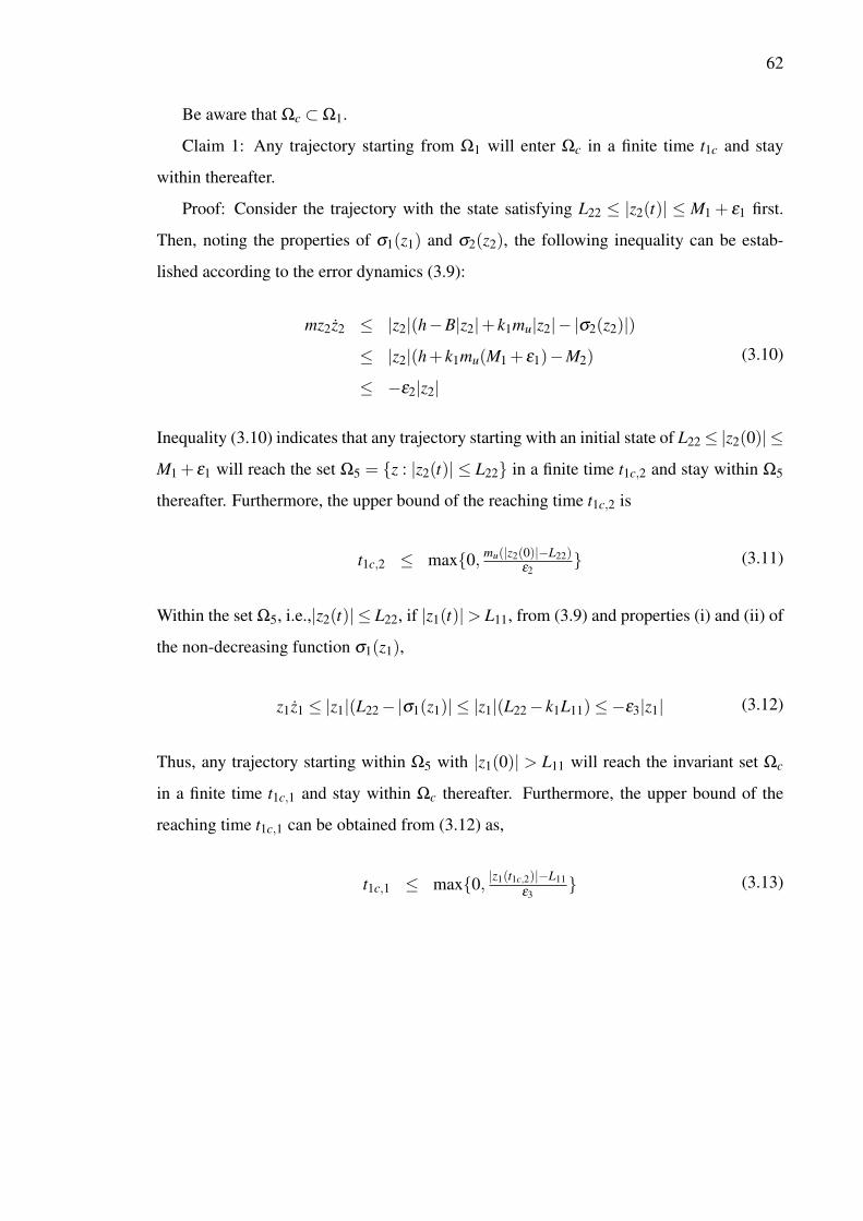
62
Be aware that Ωc ⊂Ω1.
Claim 1: Any trajectory starting from Ω1 will enter Ωc in a finite time t1c and stay
within thereafter.
Proof: Consider the trajectory with the state satisfying L22 ≤ |z2(t)| ≤ M1 + ε1 first.
Then, noting the properties of σ1(z1) and σ2(z2), the following inequality can be estab-
lished according to the error dynamics (3.9):
mz2z2 ≤ |z2|(h−B|z2|+ k1mu|z2|− |σ2(z2)|)≤ |z2|(h+ k1mu(M1 + ε1)−M2)
≤ −ε2|z2|(3.10)
Inequality (3.10) indicates that any trajectory starting with an initial state of L22 ≤ |z2(0)| ≤M1 + ε1 will reach the set Ω5 = z : |z2(t)| ≤ L22 in a finite time t1c,2 and stay within Ω5
thereafter. Furthermore, the upper bound of the reaching time t1c,2 is
t1c,2 ≤ max0, mu(|z2(0)|−L22)ε2
(3.11)
Within the set Ω5, i.e.,|z2(t)| ≤ L22, if |z1(t)|> L11, from (3.9) and properties (i) and (ii) of
the non-decreasing function σ1(z1),
z1z1 ≤ |z1|(L22−|σ1(z1)| ≤ |z1|(L22− k1L11)≤−ε3|z1| (3.12)
Thus, any trajectory starting within Ω5 with |z1(0)| > L11 will reach the invariant set Ωc
in a finite time t1c,1 and stay within Ωc thereafter. Furthermore, the upper bound of the
reaching time t1c,1 can be obtained from (3.12) as,
t1c,1 ≤ max0,|z1(t1c,2)|−L11
ε3 (3.13)

63
Combine (3.11) and (3.13), the upper bound of the reaching time for the trajectory starting
within Ω1 to Ωc is obtained
t1c = t1c,2 + t1c,1
≤ max0, mu(|z2(0)|−L22)ε2
+max0,|z1(t1c,2)|−L11
ε3
(3.14)
Claim 2: Any trajectory starting from Ω2 will enter Ω1 in a finite time t21.
Proof: In Ω2, z1z2 > 0, |z1| > L12 and |z2| > M1 + ε1 > L22. From property (iv) of σ1,∂σ1∂ z1
= 0; from property (iii) of σ2, |σ2| ≥M2. Thus, from (3.9), noting property (iii) of σ1,
z1z1 ≥ |z1|(M1 + ε1−M1)≥ ε1|z1|mz2z2 ≤ |z2|(h− (B+Fscg)|z2|−M2)≤−(M2−h)|z2|
(3.15)
which implies that in Ω2, |z1(t)| will increase but |z2(t)| will strictly decrease to M1 + ε1.
Therefore, any trajectory starting within Ω2 will reach Ω1 in a finite time t21. The upper
bound of the reaching time t21 can be obtained from (3.15) as
t21 ≤ mu(|z2(0)|−(M1+ε1))M2−h
(3.16)
Claim 3: Any trajectory starting from Ω3 will enter either Ω1 in a finite time t31, or Ω2
in a finite time t32.
Proof: In Ω3, |z1| ≤ L12 and |z2|> M1 +ε1. According to property (iii) of σ1, |σ1| ≤M1.
From (3.9), if z2 ≥M1 + ε1,
z1 = z2−σ1 ≥M1 + ε1−M1 ≥ ε1 (3.17)
and if z2 ≤−(M1 + ε1),
z1 = z2−σ1 ≤−(M1 + ε1)+M1 ≤−ε1 (3.18)

64
Equations (3.17) and (3.18) imply that, for any trajectory starting from Ω3, if it does not
enter Ω1, it will enter Ω2 in a finite time t32. The upper bound of the reaching time t32 can
be obtained as
t32 ≤ |L12sign(z2)−z1(0)|ε1
(3.19)
In this set, the dynamics of z2 is not predictable, but it is possible that the trajectory will
enter Ω1 within a finite time t31. If that happens, the reaching time t31 should be smaller
than the one obtained in (3.19), i.e., t31 ≤ t32 ≤ |L12sign(z2)−z1(0)|ε1
.
Claim 4: Any trajectory starting from Ω4 will enter either Ω1 in a finite time t41, or Ω3
in a finite time t43.
Proof: In Ω4, z1z2 < 0, |z1| > L12 and |z2| > M1 + ε1 > L22. Thus, from (3.9), if
z2 ≥M1 + ε1, z1 <−L12 and σ1 =−M1,
z1 = z2−σ1 ≥M1 + ε1 +M1 ≥ ε1 +2M1 (3.20)
and if z2 ≤−(M1 + ε1), z1 > L12 and σ1 = M1,
z1 = z2−σ1 ≤−(M1 + ε1)−M1 ≤−(ε1 +2M1) (3.21)
Thus, for any trajectory starting from Ω4, if it does not enter Ω1, it will enter Ω3 in a finite
time t43. The upper bound of the reaching time t43 can be obtained as
t43 ≤ |z1(0)|−L122M1+ε1
(3.22)
It is also possible that the trajectory will enter Ω1 within a finite time t41. If that happens,
the reaching time t41 should be smaller than the one obtained in (3.22), i.e., t41 ≤ t43 ≤|z1(0)|−L12
2M1+ε1. Another estimation of t41 could be made as follows. From property (iv) of σ1,
∂σ1∂ z1
= 0; from property (iii) of σ2, z2σ2 ≥ |z2|M2,
mz2z2 ≤ |z2|(h−M2), t41 ≤ mu(|z2(0)|−(M1+ε1))M2−h
(3.23)
65
In all, with Claim 1-4, no matter where the trajectory starts, it will enter Ωc in a finite
time and stay within thereafter. The uniformly ultimate boundedness of the closed-loop
system is thus proved.
Once the trajectory enters Ωc = z : |z1| ≤ L11, |z2| ≤ L22, the error dynamics become,
z1 = z2− k1z1
mz2 = −ϕTb θ +∆+ mxd + m∂σ1
∂ z1σ1)
−Bz2−σ2(z2)
(3.24)
Define a positive semi-definite function V2 = 12mz2
2 and let ks = k21−muk1. From the second
equation of (3.24), the derivative of V2 is given by,
V2 = mz2z2
≤ |z2|(h+mk1|z2|− k21|z2|)≤ |z2|(h− ks|z2|)≤ − ks
2 z22 +h|z2|− ks
2 z22
≤ − ks2 (|z2|− h
ks)2 + h2
2ks− ks
2 z22
≤ h2
2ks− ks
2 z22
≤ − ksmV2 + h2
2ks
(3.25)
which leads to the following inequality,
V2(t)≤ exp(−ksm t)V2(0)+ mh2
2k2s[1− exp(−ks
m t)] (3.26)
From (3.26), the steady state of z2 is bounded by |z2(∞)| ≤min hks
,L22. Then, according
to the first equation of (3.24), the final tracking error z1 is bounded by the smaller value
between hk1ks
and L11, as stated in Theorem 3.3.1. 4Now it is established that as long as the control parameters satisfy condition (a3)–(d3),
the controlled system remains stable no matter where it initially starts, no matter whether
the control input gets saturated, and all the signals are bounded. As mentioned earlier,
another online parameter estimation law is designed to identify the unknown mass in the
66
meanwhile. Once the mass estimate m∗ is obtained with good accuracy within a time period
that is short enough for further improvement to take place, another set of control parame-
ters will then be calculated online accordingly, satisfying conditions (a4) k21 > k1m∗, (b4)
k1L11 > L22, (c4) h < M2−k1M1m∗, and (d4) M2 ≤ ubd−uabd . This set of parameters could
have higher control gains (k1,k21,k22) because the uncertainty due to the unknown parame-
ters is reduced significantly, therefore the control law could switch to this set of parameters
and achieve better performance. The complete expression of control law at this stage is as
follows, with updated σ1 and σ2:
u =−ϕTb θ − dl +m∗x1d +m∗∂σ1
∂ z1σ1−σ2(z2) (3.27)
3.4 Parameter Estimation
As mentioned before, the key issue to the success of the saturation control with un-
known mass is to get accurate mass estimate quickly. In this section, a brief description
of the parameter estimation algorithm will be presented to complete this chapter. Later
a whole chapter will be dedicated to a more organized and detailed discussion on system
identification of the linear motor drive system.
The parameter estimation algorithm is composed of two parts. One is the gradient-type
adaptation law designed for the direct compensation dl so that the integral feedback could
deliver zero steady state tracking error. Furthermore, in order to guarantee the boundedness
of the parameter estimate, the commonly used projection mapping (2.9) is brought to the
adaptation law as follows:
˙dl = Pro jdl(γdlz2)
=
0 if dl = dlmax and γdlz2 > 0
0 if dl = dlmin and γdlz2 < 0
γdcz2 otherwise
(3.28)

67
where γdl is the adaptation rate of dl , dlmax and dlmin are the upper and lower bound of dl
respectively.
The other part of the estimation algorithm is to use least squares based method to cal-
culate m∗, m and θ = [B, Fsc, d0]. A well studied and commonly used method for online
adaptation is the recursive least squares method. Provided that the persistence excitation
condition is satisfied, the parameter estimate will converge to its true value with good con-
vergence rate. However, in real applications especially with control tasks going on, the
condition of persistence excitation (PE) on the regressor signals is very hard to satisfy.
Certain adjustment on the adaptation law could be made to deal with this problem. For ex-
ample, the adaptation of a particular parameter could be turned off when the corresponding
regressor is not informative enough. Simulation model has been built to check how this
method works with the proposed SARC. The parameter estimate does converge with rea-
sonably small error as expected. But overall the result is not good enough in that it takes so
much time, relatively speaking, to get good mass estimate that the switching to higher-gain
controller may never happen in a single maneuver.
Therefore, another least squares based estimate algorithm is employed to speed up the
process. Since it is of more interest to get good estimate of the unknown mass rather than
the other parameters, the following treatment has been done to achieve this goal. Remember
the equation of motion of the linear motor system and consider no unmodelled dynamics,
i.e., ∆ = 0:
mx2 +Bx2 +FscS f (x2)−d0 = u (3.29)
The system only has a high resolution position sensor. ”Back difference” it once to get x2
already introduces significant amount of noise. It is not recommended to do it twice to get
x2. A typical way to deal with this is to pass the regressors x2,x2,S f (x2),−1 and control
input u through a second order low pass filter H f 1(s) =w2
f
s2+2ζ f w f s+w2f
and get clean pseudo
acceleration signal x2 f . The system after being filtered becomes:
mx2 f +Bx2 f +FscS f f (x2)−d0 = u f (3.30)
68
where x2 f , x2 f and S f f represent the filtered signal of x2, x2 and S f respectively. Notice
that among the four regressors, 1 is a constant and S f f (x2) which approximate the Coulomb
friction is almost a constant when the system moves except for direction changing period.
Therefore, a high pass filter H f 2(s) = τ f sτ f s+1 could be used to remove the effect caused by
the Coulomb friction and the constant disturbance d0 and further simplify the equation as
follows,
mx2 f f +Bx2 f f ≈ u f f (3.31)
where x2 f f and x2 f f are the further filtered signals. The ”≈” accounts for the modelling
error when the system starts moving and when it changes direction due to the non-constant
Coulomb friction during those periods. With (3.31) there are two regressors remain so
the PE condition is easy to satisfy. In addition, collecting reasonable amount of data and
performing standard least squares calculation is convenient to carry out. For example,
starting from time zero N samples have been collected as x2 f f (1,2, ...,N),x2 f f (1,2, ...,N)
and u f f (1,2, ...,N). The estimate would then be calculated as:
m∗
B∗
=
∑N
i=1 x22 f f (i) ∑N
i=1 x2 f f (i)x2 f f (i)
∑Ni=1 x2 f f (i)x2 f f (i) ∑N
i=1 x22 f f (i)
−1
∑Ni=1 x2 f f (i)u f f (i)
∑Ni=1 x2 f f (i)u f f (i)
(3.32)
Since the least squares method intends to average out the modelling error, the mass estimate
could be expected to have reasonably good accuracy even with the unmodelled dynamics
(∆ 6= 0) and the approximation of the Coulomb friction concerned. How to pick the number
of samples N so that the collection is large enough and rich enough depends on the real
application. In addition, the calculated estimate will be cut off at the preset boundary ml
and mu to ensure Property (P1).
A quicker and more accurate mass estimate m∗ is obtained in the way described above
to replace the previously estimated m, whereas m is obtained together with the other three
system parameters θ = [B,Fsc,d0] using the standard recursive least squares method with
the projection mapping.
69
3.5 Hardware Experiments
The test bed for this algorithm is again the Y-axis linear motor drive system shown in
Fig. 2.5. The control input gain K f is 27.79N/V and the input voltage through the D/A
port is capped at±10V , which makes the saturation level of the driving force ubd = 277.9N.
The sampling frequency is 2.5kHz. The resolution of the position encoder is 1µm and the
velocity feedback is calculated by the ”back difference” of the position signal. The mass of
the moving stage with no load is 3.34kg. For the sake of simplicity, instead of physically
adding different load, different ranges of parameter uncertainty are employed to cover the
situations that the unknown mass is (a) close to the lower bound m ∈ [3.2,12.4]; (b) in the
middle of the range m ∈ [1.5,6]; or (c) close to the upper bound m ∈ [1,4]. For all three
situations, the upper bound is approximately four times the lower bound.
As to the desired trajectory for the system to follow, both the commonly used point-
to-point movement and the extreme step-like trajectory are applied as in Chapter 2, except
that online trajectory replanning is carried out for the step-like trajectory to further improve
the performance. More details will be revealed in the following.
3.5.1 Point-To-Point Trajectory
In general, planning the desired trajectory should be very careful especially when the
mass is unknown. It should make sure that the maximum acceleration is feasible even for
the maximum load possible, and the maximum velocity is within the detectable scope of
the position sensor. The type of the point-to-point trajectory used here has appeared in last
chapter. It is at least twice continuously differentiable. For mass range (a) with upper bound
mu = 12.4kg, the trajectory is planned having a distance of 0.4m, a maximum velocity of
0.8m/s and a maximum acceleration of 4m/s2 as shown in Fig. 3.1. For mass range (b)
with upper bound mu = 6kg, the trajectory is planned with a distance of 0.4m, a maximum
velocity of 1m/s and a maximum acceleration of 8m/s2 as shown in Fig. 3.2. For mass
range (c) with upper bound mu = 4kg, the trajectory is planned with a distance of 0.4m,
a maximum velocity of 1m/s and a maximum acceleration of 12m/s2 as shown in Fig.

70
0 2 4 6 8 10 12 14 16 18 200
0.1
0.2
0.3
0.4
Time (sec
Des
ired
Pos
ition
(m
)
0 2 4 6 8 10 12 14 16 18 20−1
−0.5
0
0.5
1
Time
Des
ired
Vel
ocity
(m
/s)
0 2 4 6 8 10 12 14 16 18 20−4
−2
0
2
4
Time
Des
ired
Acc
eler
atio
n (m
/s2 )
Figure 3.1. Point-to-point trajectory for mass range (a)[3.2,12.4].
3.3. The trajectory at each sampling period is calculated in advance and keeps the same
way before and after the mass is estimated. The main objective for this set of experiments
is to show the process of the system switching from conservative control parameters to
aggressive ones once a good mass estimate is obtained.
The control parameters are also different for mass range (a), (b) and (c) due to different
upper bound mu, but both have to satisfy the design constraints (a3)–(d3) before and (a4)–
(d4) after the mass estimate m∗ is provided.
The tracking performance of the controlled system is shown in the following figures.
Fig. 3.4 - Fig. 3.6 show the whole switching process of the system between two sets
of control parameters for three different mass ranges. The mass estimate is obtained at
around 1 second after the system starts and the estimated value is (a)3.27kg,(b)3.08kg
and (c)3.22kg, quite close to the nominal value 3.34kg. After that moment, significant
improvement on the tracking error could be observed from the figures because not only

71
0 2 4 6 8 10 12 14 16 18 200
0.1
0.2
0.3
0.4
Time (sec
Des
ired
Pos
ition
(m
)
0 2 4 6 8 10 12 14 16 18 20−1
−0.5
0
0.5
1
Time
Des
ired
Vel
ocity
(m
/s)
0 2 4 6 8 10 12 14 16 18 20−10
−5
0
5
10
Time
Des
ired
Acc
eler
atio
n (m
/s2 )
Figure 3.2. Point-to-point trajectory for mass range (b)[1.5,6].
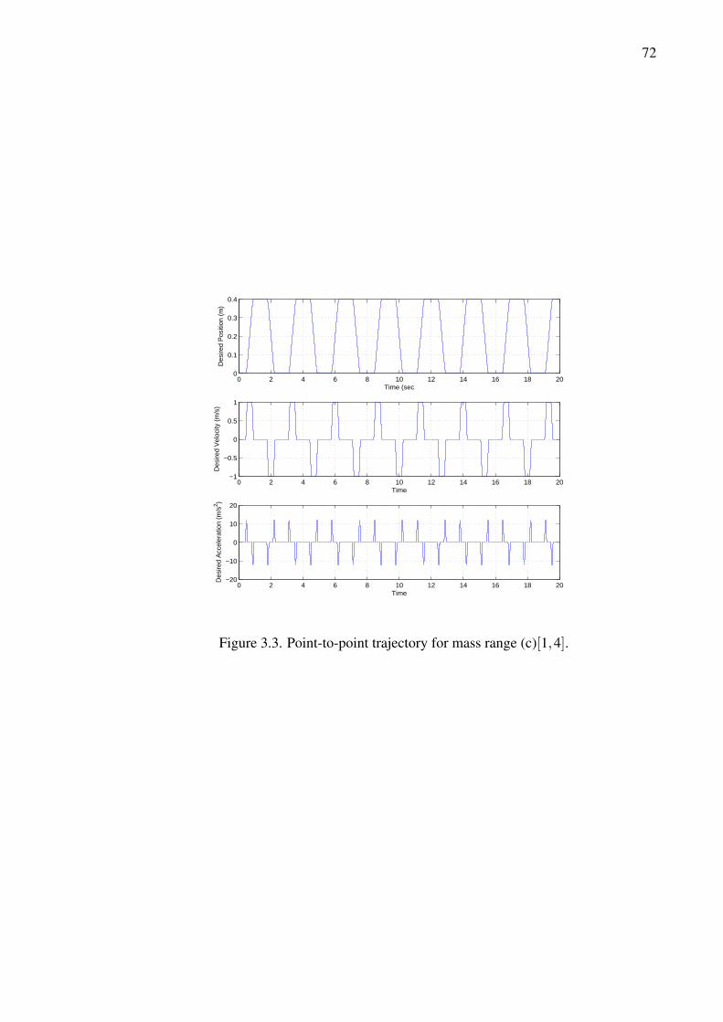
72
0 2 4 6 8 10 12 14 16 18 200
0.1
0.2
0.3
0.4
Time (sec
Des
ired
Pos
ition
(m
)
0 2 4 6 8 10 12 14 16 18 20−1
−0.5
0
0.5
1
Time
Des
ired
Vel
ocity
(m
/s)
0 2 4 6 8 10 12 14 16 18 20−20
−10
0
10
20
Time
Des
ired
Acc
eler
atio
n (m
/s2 )
Figure 3.3. Point-to-point trajectory for mass range (c)[1,4].

73
0 2 4 6 8 10 12 14 16 18 20−4
−3
−2
−1
0
1
2
3x 10
−5
Time (sec)
Trac
king
Erro
r (m
)
0 2 4 6 8 10 12 14 16 18 20−4
−3
−2
−1
0
1
2
3
4
Time (sec)
Cont
rol I
nput
(V)
Figure 3.4. P2P tracking performance of mass range (a)[3.34,12.4].
0 2 4 6 8 10 12 14 16 18 20−1
−0.5
0
0.5
1x 10
−4
Time (sec)
Trac
king
Erro
r (m
)
0 2 4 6 8 10 12 14 16 18 20−6
−4
−2
0
2
4
Time (sec)
Cont
rol I
nput
(V)
Figure 3.5. P2P tracking performance of mass range (b)[1.5,6].
the controller gets updated with higher gains but the uncertainty level due to the unknown
parameters is also reduced.

74
0 2 4 6 8 10 12 14 16 18 20−2
−1.5
−1
−0.5
0
0.5
1
1.5x 10
−4
Time (sec)
Trac
king
Erro
r (m
)
0 2 4 6 8 10 12 14 16 18 20−5
0
5
Time (sec)
Cont
rol I
nput
(V)
Figure 3.6. P2P tracking performance of mass range (c)[1,4].

75
6.5 7 7.5 8 8.5 9−2
−1.5
−1
−0.5
0
0.5
1
1.5
2x 10
−5
Time (sec)Tr
ackin
g Er
ror (
m)
6.5 7 7.5 8 8.5 9−4
−3
−2
−1
0
1
2
3
4
Time (sec)
Cont
rol I
nput
(V)
Figure 3.7. P2P tracking performance (zoomed in) of mass range (a)[3.34,12.4].
A zoomed-in version of one period randomly picked after when the mass is estimated is
shown in Fig. 3.7 - Fig. 3.9. There is only slight difference among the performance of three
mass ranges mainly due to the different acceleration level of the desired trajectory. For all
three cases, the tracking errors during acceleration/deceleration periods are within 20µm,
during constant speed periods are around 5µm and during zero speed periods are zero
thanks to the dl compensation. Since the desired trajectories are planned to be within the
authority of the control input, the controlled system’s ability to deal with input saturation
is not shown in this set of experiment. But it does meet the objective to demonstrate the
success of the switching control law.
3.5.2 Step-like Trajectory
In some industrial applications, an object needs to be transported from one point to
another by for instance, a linear motor positioning system. It is a one-direction movement.
Less travel time and smaller overshoot/vibration around the set point are the most important
requirements for the controller design. In order to achieve less travel time, an engineer with

76
5.8 6 6.2 6.4 6.6 6.8 7 7.2 7.4 7.6 7.8−2
−1.5
−1
−0.5
0
0.5
1
1.5
2x 10
−5
Time (sec)
Trac
king
Erro
r (m
)
5.8 6 6.2 6.4 6.6 6.8 7 7.2 7.4 7.6 7.8−5
0
5
Time (sec)
Cont
rol I
nput
(V)
Figure 3.8. P2P tracking performance (zoomed in) of mass range (b)[1.5,6].
5.6 5.8 6 6.2 6.4 6.6 6.8 7 7.2 7.4 7.6−2
−1.5
−1
−0.5
0
0.5
1
1.5
2x 10
−5
Time (sec)
Trac
king
Erro
r (m
)
5.6 5.8 6 6.2 6.4 6.6 6.8 7 7.2 7.4 7.6−5
0
5
Time (sec)
Cont
rol I
nput
(V)
Figure 3.9. P2P tracking performance (zoomed in) of mass range (c)[1,4].
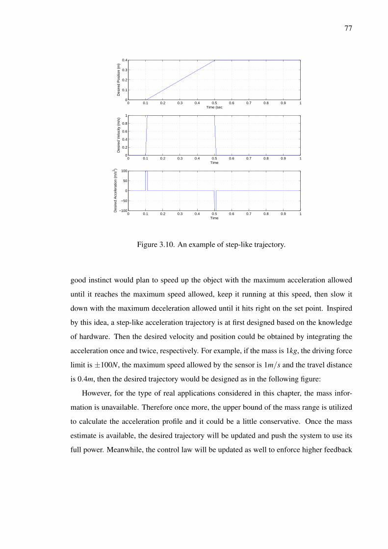
77
0 0.1 0.2 0.3 0.4 0.5 0.6 0.7 0.8 0.9 10
0.1
0.2
0.3
0.4
Time (sec
Des
ired
Pos
ition
(m
)
0 0.1 0.2 0.3 0.4 0.5 0.6 0.7 0.8 0.9 10
0.2
0.4
0.6
0.8
1
Time
Des
ired
Vel
ocity
(m
/s)
0 0.1 0.2 0.3 0.4 0.5 0.6 0.7 0.8 0.9 1−100
−50
0
50
100
Time
Des
ired
Acc
eler
atio
n (m
/s2 )
Figure 3.10. An example of step-like trajectory.
good instinct would plan to speed up the object with the maximum acceleration allowed
until it reaches the maximum speed allowed, keep it running at this speed, then slow it
down with the maximum deceleration allowed until it hits right on the set point. Inspired
by this idea, a step-like acceleration trajectory is at first designed based on the knowledge
of hardware. Then the desired velocity and position could be obtained by integrating the
acceleration once and twice, respectively. For example, if the mass is 1kg, the driving force
limit is ±100N, the maximum speed allowed by the sensor is 1m/s and the travel distance
is 0.4m, then the desired trajectory would be designed as in the following figure:
However, for the type of real applications considered in this chapter, the mass infor-
mation is unavailable. Therefore once more, the upper bound of the mass range is utilized
to calculate the acceleration profile and it could be a little conservative. Once the mass
estimate is available, the desired trajectory will be updated and push the system to use its
full power. Meanwhile, the control law will be updated as well to enforce higher feedback
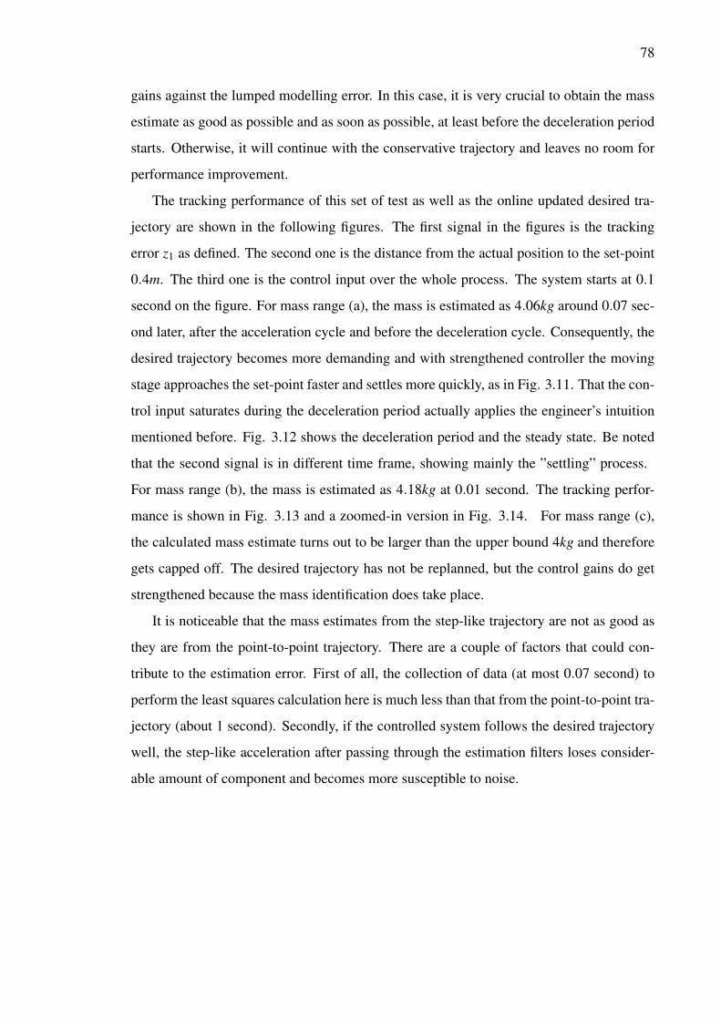
78
gains against the lumped modelling error. In this case, it is very crucial to obtain the mass
estimate as good as possible and as soon as possible, at least before the deceleration period
starts. Otherwise, it will continue with the conservative trajectory and leaves no room for
performance improvement.
The tracking performance of this set of test as well as the online updated desired tra-
jectory are shown in the following figures. The first signal in the figures is the tracking
error z1 as defined. The second one is the distance from the actual position to the set-point
0.4m. The third one is the control input over the whole process. The system starts at 0.1
second on the figure. For mass range (a), the mass is estimated as 4.06kg around 0.07 sec-
ond later, after the acceleration cycle and before the deceleration cycle. Consequently, the
desired trajectory becomes more demanding and with strengthened controller the moving
stage approaches the set-point faster and settles more quickly, as in Fig. 3.11. That the con-
trol input saturates during the deceleration period actually applies the engineer’s intuition
mentioned before. Fig. 3.12 shows the deceleration period and the steady state. Be noted
that the second signal is in different time frame, showing mainly the ”settling” process.
For mass range (b), the mass is estimated as 4.18kg at 0.01 second. The tracking perfor-
mance is shown in Fig. 3.13 and a zoomed-in version in Fig. 3.14. For mass range (c),
the calculated mass estimate turns out to be larger than the upper bound 4kg and therefore
gets capped off. The desired trajectory has not be replanned, but the control gains do get
strengthened because the mass identification does take place.
It is noticeable that the mass estimates from the step-like trajectory are not as good as
they are from the point-to-point trajectory. There are a couple of factors that could con-
tribute to the estimation error. First of all, the collection of data (at most 0.07 second) to
perform the least squares calculation here is much less than that from the point-to-point tra-
jectory (about 1 second). Secondly, if the controlled system follows the desired trajectory
well, the step-like acceleration after passing through the estimation filters loses consider-
able amount of component and becomes more susceptible to noise.
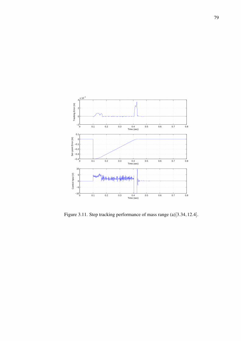
79
0 0.1 0.2 0.3 0.4 0.5 0.6 0.7 0.8−2
0
2
4x 10
−4
Time (sec)
Tra
ckin
g E
rror
(m
)
0 0.1 0.2 0.3 0.4 0.5 0.6 0.7 0.8−0.4
−0.3
−0.2
−0.1
0
0.1
Time (sec)
Set
−poi
nt E
rror
(m
)
0 0.1 0.2 0.3 0.4 0.5 0.6 0.7 0.8−10
−5
0
5
10
Time (sec)
Con
trol
Inpu
t (V
)
Figure 3.11. Step tracking performance of mass range (a)[3.34,12.4].

80
0.4 0.42 0.44 0.46 0.48 0.5 0.52 0.54−2
0
2
4x 10
−4
Time (sec)
Tra
ckin
g E
rror
(m
)
0.44 0.45 0.46 0.47 0.48 0.49 0.5 0.51 0.52 0.53 0.54−5
0
5
10x 10
−6
Time (sec)
Set
−poi
nt E
rror
(m
)
0.4 0.42 0.44 0.46 0.48 0.5 0.52 0.54−10
−5
0
5
10
Time (sec)
Con
trol
Inpu
t (V
)
Figure 3.12. Step tracking performance (zoomed in) of mass range (a)[3.34,12.4].

81
0 0.1 0.2 0.3 0.4 0.5 0.6 0.7 0.8−4
−3
−2
−1
0
1x 10
−3
Time (sec)
Tra
ckin
g E
rror
(m
)
0 0.1 0.2 0.3 0.4 0.5 0.6 0.7 0.8−0.4
−0.3
−0.2
−0.1
0
0.1
Time (sec)
Set
−poi
nt E
rror
(m
)
0 0.1 0.2 0.3 0.4 0.5 0.6 0.7 0.8−10
−5
0
5
10
Time (sec)
Con
trol
Inpu
t (V
)
Figure 3.13. Step tracking performance of mass range (b)[1.5,6].
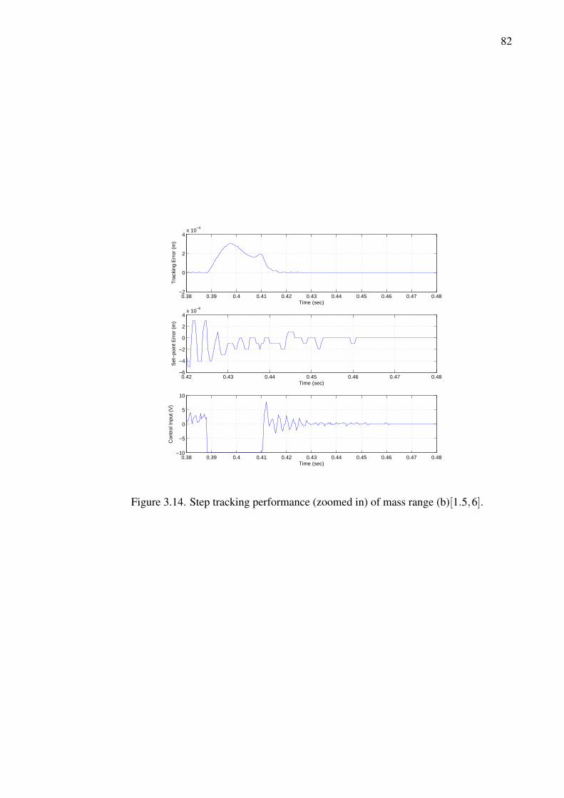
82
0.38 0.39 0.4 0.41 0.42 0.43 0.44 0.45 0.46 0.47 0.48−2
0
2
4x 10
−4
Time (sec)
Tra
ckin
g E
rror
(m
)
0.42 0.43 0.44 0.45 0.46 0.47 0.48−6
−4
−2
0
2
4x 10
−6
Time (sec)
Set
−poi
nt E
rror
(m
)
0.38 0.39 0.4 0.41 0.42 0.43 0.44 0.45 0.46 0.47 0.48−10
−5
0
5
10
Time (sec)
Con
trol
Inpu
t (V
)
Figure 3.14. Step tracking performance (zoomed in) of mass range (b)[1.5,6].

83
0 0.1 0.2 0.3 0.4 0.5 0.6 0.7 0.8−8
−6
−4
−2
0
2x 10
−3
Time (sec)
Tra
ckin
g E
rror
(m
)
0 0.1 0.2 0.3 0.4 0.5 0.6 0.7 0.8−0.4
−0.3
−0.2
−0.1
0
0.1
Time (sec)
Set
−poi
nt E
rror
(m
)
0 0.1 0.2 0.3 0.4 0.5 0.6 0.7 0.8−10
−5
0
5
10
Time (sec)
Con
trol
Inpu
t (V
)
Figure 3.15. Step tracking performance of mass range (c)[1,4].
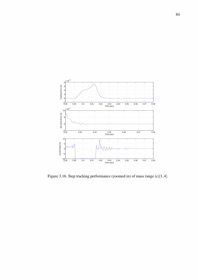
84
0.38 0.39 0.4 0.41 0.42 0.43 0.44 0.45 0.46 0.47 0.48−2
0
2
4
6
8x 10
−4
Time (sec)
Tra
ckin
g E
rror
(m
)
0.42 0.43 0.44 0.45 0.46 0.47 0.48−5
0
5
10x 10
−5
Time (sec)
Set
−poi
nt E
rror
(m
)
0.38 0.39 0.4 0.41 0.42 0.43 0.44 0.45 0.46 0.47 0.48−10
−5
0
5
10
Time (sec)
Con
trol
Inpu
t (V
)
Figure 3.16. Step tracking performance (zoomed in) of mass range (c)[1,4].
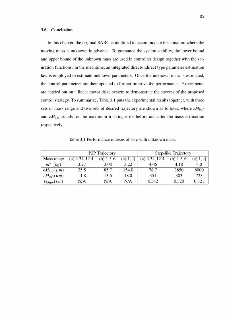
85
3.6 Conclusion
In this chapter, the original SARC is modified to accommodate the situation where the
moving mass is unknown in advance. To guarantee the system stability, the lower bound
and upper bound of the unknown mass are used in controller design together with the sat-
uration functions. In the meantime, an integrated direct/indirect type parameter estimation
law is employed to estimate unknown parameters. Once the unknown mass is estimated,
the control parameters are then updated to further improve the performance. Experiments
are carried out on a linear motor drive system to demonstrate the success of the proposed
control strategy. To summarize, Table 3.1 puts the experimental results together, with three
sets of mass range and two sets of desired trajectory are shown as follows, where eMbe f
and eMa f t stands for the maximum tracking error before and after the mass estimation
respectively.
Table 3.1 Performance indexes of sarc with unknown mass.
P2P Trajectory Step-like TrajectoryMass range (a)[3.34,12.4] (b)[1.5,6] (c)[1,4] (a)[3.34,12.4] (b)[1.5,6] (c)[1,4]
m∗ (kg) 3.27 3.08 3.22 4.06 4.18 4.0eMbe f (µm) 35.5 85.7 154.0 76.7 3850 8000eMa f t(µm) 11.8 13.6 18.0 351 303 723ts5µm(sec) N/A N/A N/A 0.342 0.320 0.321

86
4. SYSTEM IDENTIFICATION OF THE LINEAR MOTOR DRIVE SYSTEM
System identification (ID) is such a huge topic that no one would attempt to cover all
the bases in just a single chapter. There are so many research papers and mathematical
algorithms developed to help people get to know physical systems better. In general, system
ID is the first step to study a system no matter what the following research questions are.
Therefore, the linear motor drive system for which the saturated adaptive control law is
designed has been studied thoroughly with both offline and online experiments carried
out as part of the system ID process. Although all the equations and algorithms such as
gradient type adaptation law or least squares method are well known and commonly used,
how to use them effectively under different situations to achieve different objectives is
not trivial or easy. In this chapter, elaborate discussion will be brought on this topic and
certain modification on some popular estimation algorithms for real-time application will
be introduced.
4.1 Offline Parameter Adaptation
For the linear motor system, a typical second order system, it is easy to obtain its model
structure as follows:
mx+Bx+FscS f (x)+d0 +∆(t) = K f u (4.1)
where x is the displacement of the moving stage which is measurable and u is the control in-
put to the system which is calculable. m is the mass of the moving stage plus whatever load
it may carry with. K f is the input gain from the input voltage to the magnetic force driving
the stage. B and Fsc represent two major friction coefficients, viscous and Coulomb respec-
tively to model the total friction force. d0 and ∆ represent the low frequency (or constant
part) and high frequency components of the lumped unmodelled dynamics plus external
disturbance. S f (x) is a continuous function used to capture the shape of the highly non-
87
linear Coulomb friction and the discrepancy between them is lumped into term ∆. Model
(4.1) is a good one to describe the system because (a) it captures the majority of the physi-
cal characteristics of this linear motor and (b) the complexity level of the model is suitable
for future controller design.
Remark 1 There are a lot of friction models in the literature and the one used here
(Coulomb plus viscous) is among the earliest and simplest. A sophisticated dynamic fric-
tion model will be introduced in next chapter and simulation results demonstrates that it
models friction much more accurately for slow motion and direction change period. How-
ever, the advantage of this dynamic friction model won’t be able to get recognized in real-
time experiments because the resolution of the position encoder is 1µm which is not high
enough to appreciate the difference between these two friction models. Therefore, the
Coulomb-viscous friction model is utilized throughout the system ID process and the con-
troller design afterwards.
Now that the model structure has been figured out following physical principles, the
remainder of the system ID procedure is to obtain the parameters m,B,Fsc,d0 and K f and
to determine the bound of the lumped unmodelled dynamics ∆ under normal working con-
dition. Among these system parameters, the mass m and input gain K f can be roughly
estimated from the manufacturer data and the measurements of a test point of the power
amplifier. The rest of them are rather difficult to fix. For example, although friction coeffi-
cients are rather steady during a single test period, they are likely to vary over a long period
of time, different temperature, humidity or lubricant condition. Therefore, offline parame-
ter estimation is necessary to determine the nominal value of these system parameters and
it needs to be conducted on a regular base to maintain the good condition of the equipment.
In addition, since it is easy to control the signal condition in offline experiments, exten-
sive test results under different conditions could be obtained to set up a range of parameter
variation, for ARC control design.
As to the offline parameter estimation technique, least squares method is a typical
choice since the unknown parameters are linearly distributed in the equation. However

88
it is obvious that they can not be identified at the same time. The equation of motion is then
rewritten as:mkx+Bkx+FsckS f (x)+d0k +∆k(t) = u
ϕ(x)T θ +∆k = u(4.2)
where ϕ(x) = [x, x,S f (x),1]T are the regressors need to obtain from the measurement.
θ = [mk,Bk,Fsck,d0k]T = [m,B,Fsc,d0]T /K f is the normalized parameters with respect to
the input gain K f . Real-time experiments are designed in the following to get the parameter
estimate θ and the modelling error ∆k(t) can be analyzed consequently. Next, these exper-
iments will be carried out again with a load weighing 9.06kg (20lb) added to the moving
stage and the same set of parameters are estimated as θl = [mkl,Bkl,Fsckl,d0kl]T . Since it is
known that mkl = mk + 9.06K f
, according to the estimates of mkl and mk, K f can be calculated.
Thus, all system parameters are obtained.
There are a couple of issues need taken care of while designing the experiments for sys-
tem ID. First, as mentioned earlier, input and output signals are collected to perform least
squares. These signals, or at least some segments of these signals, will form the regressor
which should satisfy the persistence excitation (PE) condition in order to get good parame-
ter estimation. Therefore, input signal should be designed to trigger informative responses.
In more detail, the acceleration and velocity signals should have enough variation so that
the signals which form the regressor are uncorrelated. If the system is open loop stable
like this case, it is feasible and easy to design input signal to excite the system. Otherwise,
a stabilizing controller in a closed-loop structure needs to be designed beforehand, which
adds a little difficulty to make regressors informative.
Second, the equipped sensor only provides the displacement of the stage. To obtain its
velocity, ”back difference” is conducted once on the position signal and it introduce quite
a bit noise. It is even worse to ”back difference” position twice to get the acceleration. A
better way to solve this problem is to pass both sides of the equation (4.2) through a low

89
pass filter with the cut-off frequency high enough not to interfere with the system dynamics.
Then the equation becomes:
mkx f +Bkx f +FsckS f f (x)+d0k +∆k f (t) = u f
ϕTf θ +∆k f = u f
(4.3)
The input signal u(t) is chosen to be a square wave. With different amplitude and fre-
quency, it can produce back and forth movements with different speed and acceleration
to cover normal working condition. In case some application may require one direction
movement, such trajectory is also designed to investigate this situation. Notice that regres-
sor S f f (x) would be almost like a constant during one direction movement, it is difficult
to differentiate parameter Fsck and d0k from each other. Therefore, a proper way to con-
tinue system ID is to lump these two terms together and estimate the total effect. Table 4.1
summarizes different square-wave inputs with corresponding system outputs with different
velocity and acceleration.
Table 4.1 Offline system ID: input and output signals.
Input \ Output Max accel. (m/s2) Max vel. (m/s) Change direction?Normal 1V,2Hz 14.9 0.47 YesLow 0.4V,1Hz 4.2 0.13 YesHigh 2V,2Hz 30.8 1.32 Yes
One direction 0.8V,0.1Hz 1.9 0.29 No
For illustration purpose, the regressors resulting from the ”Normal” input is shown in
Fig. 4.1 as an example and the zoomed in portion of one second data is shown in Fig. 4.2.
As mentioned before, the collection of data should be large and rich enough to perform
the least squares estimate, i.e., the four regressor arrays should be linear independent. 10
second data obtained from Fig. 4.1 certainly satisfy the PE condition. The parameter
estimation calculated from this set of data is:
θ = [0.1173 1.7427 0.2673 0.0536]T .

90
22 23 24 25 26 27 28 29 30 31 32−20
0
20
Time (sec)
Filt
ere
d a
cce
lera
tio
n
22 23 24 25 26 27 28 29 30 31 32−0.5
0
0.5
Time (sec)
Filt
ere
d v
elo
city
22 23 24 25 26 27 28 29 30 31 32−1
0
1
Time (sec)
Filt
ere
d C
ou
lom
b f
rictio
n
22 23 24 25 26 27 28 29 30 31 320
1
2
Time (sec)
Filt
ere
d o
ne
Figure 4.1. Regressors resulting from ”Normal” square wave input (10 secand without load).

91
24 24.1 24.2 24.3 24.4 24.5 24.6 24.7 24.8 24.9 25−20
0
20
Time (sec)
Filt
ere
d a
cce
lera
tio
n
24 24.1 24.2 24.3 24.4 24.5 24.6 24.7 24.8 24.9 25−0.5
0
0.5
Time (sec)
Filt
ere
d v
elo
city
24 24.1 24.2 24.3 24.4 24.5 24.6 24.7 24.8 24.9 25−1
0
1
Time (sec)
Filt
ere
d C
ou
lom
b f
rictio
n
24 24.1 24.2 24.3 24.4 24.5 24.6 24.7 24.8 24.9 250
1
2
Time (sec)
Filt
ere
d o
ne
Figure 4.2. Regressors resulting from ”Normal” square wave input (1 secand without load).

92
22 23 24 25 26 27 28 29 30 31 32−1.5
−1
−0.5
0
0.5
1
1.5
estim
ated
and
acu
tal u
f (V)
22 23 24 25 26 27 28 29 30 31 32−0.6
−0.4
−0.2
0
0.2
0.4
time (sec)
inpu
t est
imat
ion
erro
r (V)
estimatedactual
Figure 4.3. Modelling error resulting from ”Normal” square wave input (without load).
In fact, any data section involving the direction change period would satisfy the PE con-
dition. Therefore, 10 segments of data with 1 second each are picked to perform least
squares calculation. The average of the estimation is very close to what has been found
with 10 second data:
θ = [0.1165 1.8608 0.2608 0.0487]T .
With these results, the modelling error ∆ f (t) could be characterized as ∆ f = u f −ϕTf θ and
shown in Fig. 4.3 Following the same procedure, the analysis of data from ”low”, ”high”
and ”one direction” control inputs give similar parameter estimates and provide the range
of parameter variation and the bound of modelling error.
The second part of the offline experiment is to repeat the above tests and analysis for the
system with 20lb load carried on. Take the ”Normal” input as an example, the parameter
estimate obtain from 10 second data collection as in Fig. 4.4 is
θl = [0.4357 1.3227 0.3676 0.0165]T .

93
25 26 27 28 29 30 31 32 33 34 35−10
0
10
Time (sec)
Filt
ere
d a
cce
lera
tio
n
25 26 27 28 29 30 31 32 33 34 35−1
0
1
Time (sec)
Filt
ere
d v
elo
city
25 26 27 28 29 30 31 32 33 34 35−1
0
1
Time (sec)
Filt
ere
d C
ou
lom
b f
rictio
n
25 26 27 28 29 30 31 32 33 34 350
1
2
Time (sec)
Filt
ere
d o
ne
Figure 4.4. Regressors resulting from ”Normal” square wave input (10 sec and with load).
and the average estimate from 10 segments of 1 second data as in Fig. 4.5 is
θl = [0.4399 1.2975 0.3848 0.0137]T .
The corresponding modelling error is calculated as in Fig. 4.6
Now that the mass estimate for both cases – 0.1165 without the load and 0.4399 with
the load are obtained, the control input gain K f is calculated as 28.05, very close to the
number from the manufacturer sheet 27.79.
In summary, with the offline system ID procedure, a mathematical model to describe the
physical system is obtained. The system parameters are estimated under different working
conditions. Their nominal values are obtained and a range of variation for each parameter

94
24 24.1 24.2 24.3 24.4 24.5 24.6 24.7 24.8 24.9 25−10
0
10
Time (sec)
Filt
ere
d a
cce
lera
tio
n
24 24.1 24.2 24.3 24.4 24.5 24.6 24.7 24.8 24.9 25−1
0
1
Time (sec)
Filt
ere
d v
elo
city
24 24.1 24.2 24.3 24.4 24.5 24.6 24.7 24.8 24.9 25−1
0
1
Time (sec)
Filt
ere
d C
ou
lom
b f
rictio
n
24 24.1 24.2 24.3 24.4 24.5 24.6 24.7 24.8 24.9 250
1
2
Time (sec)
Filt
ere
d o
ne
Figure 4.5. Regressors resulting from ”Normal” square wave input (1 sec and with load).
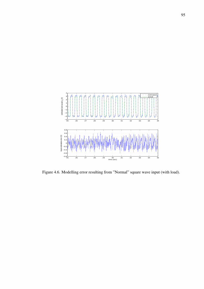
95
25 26 27 28 29 30 31 32 33 34 35−4
−3
−2
−1
0
1
2
3
4
estim
ated
and
acu
tal u
f (V)
estimatedactual
25 26 27 28 29 30 31 32 33 34 35−0.8
−0.6
−0.4
−0.2
0
0.2
0.4
0.6
0.8
time (sec)
inpu
t est
imat
ion
erro
r (V)
Figure 4.6. Modelling error resulting from ”Normal” square wave input (with load).

96
has been set. As to the unmodelled dynamics ∆(t), the bound of its amplitude has been cal-
culated although its structure remains unknown. These results are very valuable for future
controller design, such as the adaptive robust control design which needs the knowledge of
the extend of parameter variation in prior.
4.2 Online Parameter Adaptation
Another important application of system Id is to provide online parameter estimation
to construct the model compensation part of the control input, which helps reduce the
modelling error and achieve better tracking performance. Depending on the application for
which the control law is designed, different types of adaptation law have been investigated
and applied. For example, if the sole control objective is to minimize the tracking error, the
gradient type direct parameter adaptation is a good choice because it is easy to implement
and asymptotic tracking can be achieved if there is no unmodelled dynamics, i.e., ∆ = 0. On
the other hand, if accurate parameter estimate is of great interest, the least squares indirect
adaptation law have a better chance to achieve this goal but the computational burden is
much higher. A combination of both methods called integrated direct/indirect adaptation
law provides good parameter estimation and helps reduce tracking error as well, again the
computation efficiency may be an issue. Test results comparing these three methods will
be shown in the following.
4.2.1 Gradient Type Direct Adaptation
This adaptation law has been used widely in adaptive control techniques where online
parameter estimates are needed for model compensation. The standard design procedure is
to set˙θ = Γτ (4.4)
where θ is the parameter estimate, Γ is the adaptation gain and τ is the tuning function
which would be determined later. We want to select control input u and tuning function τ

97
to guarantee the derivative of a Lyapunov function is non-positive. For example if the error
dynamics after the controller is designed and plugged in becomes:
z =−kz−ϕ(x)T θ (4.5)
where k is the feedback gain and θ = θ − θ , therefore ˙θ = ˙θ . We choose the Lyapunov
function candidate to be
V (t) =12
z2 + θ T Γ−1θ
then
V = zz+ θ T τ =−kz2− zϕ(x)T θ + θ T τ
. At this stage, the tuning function τ would be set as τ = ϕ(x)z so that it will cancel the
term −zϕ(x)T θ and make V negative semi-definite.
This estimation law is easy to design and implement. The adaptation gain Γ is the
design parameter which may need some extra care because it will affect the closed loop
system bandwidth in certain cases. Take system (4.5) as an example, it could be rewritten
as:
z =−kz−ϕ(x)T (θ(0)+∫
Γϕ(x)zdt) (4.6)
If the regressor is slowly varying signals compare to desired closed-loop bandwidth, the
above equation could be approximated as:
z≈−kz−ϕ(x)T Γϕ(x)∫
zdt +Constant (4.7)
Now the error dynamics has a proportional and integral feedback with ϕ(x)T Γϕ(x) being
the integral gain. The closed-loop system bandwidth is determined not only by k, but also
by Γ. Meanwhile the tracking performance gets improved because of the integral action.
This issue is recognized in our SARC design described in Chapter 2. Since there is a
constant 1 in the regressors corresponding to the low frequency component d0, we choose
its adaptation gain together with feedback gains k1,k21 to get desirable closed-loop band-

98
width and keep the other adaptation gains very small, which raises the second issue about
this algorithm – the parameter estimate doesn’t converge in general.
The main reason that the estimate seldom converges is because the driving signal for
the adaptation law (4.4) is the tracking error z , which would be very small and corrupted
by noise if the controller is doing a good job. Furthermore, the choice of adaptation gain Γ
is limited by the first issue. Therefore, some of the parameters may get updated very slowly
and never converge to its true value.
4.2.2 Recursive Least Squares Indirect Adaptation
The indirect adaptation method is most applied to the design problems which require
accurate parameter estimation for further diagnostic purpose. Basically, it utilizes the orig-
inal system dynamics instead of the error dynamics and its design is independent on the
control design. Both gradient and least squares type algorithm could be used to get pa-
rameter estimate. In general, least squares method has better convergence property and
therefore is more popular.
The detailed procedure and the mathematical equations could be found in [16]. The
focus here is to discuss how to deal with the PE condition in real-time application. Re-
gardless which adaptation method to use, only when the persistence excitation condition is
satisfied can the parameter estimate converges to true value. However, since the experiment
condition is hard to manage with the main control loop working aside, maintaining the full
rank of the covariance matrix even for a short period of time might be very difficult. There-
fore, an ”ad-hoc” adjustment is made on the implementation of the recursive least squares
algorithm to improve the convergence of the estimate.
Take the linear motor point to point tracking control for example. The desired trajectory
is planned in advance and we assume the actual state will follow the desired trajectory
closely, thus we could predict that for each parameter, the corresponding regressor is going
to be active during certain time periods ta and passive during other time periods tp. Then the
parameter will get updated according to the recursive algorithm during time ta and remain

99
unchanged during time tp. The experimental results with this adjustment shows that the
parameter estimate does converge, but not exactly to the true value due to the unmodelling
dynamics ∆.
4.2.3 Integrated Direct/Indirect Adaptation
The indirect adaptation method is good at parameter estimation, but it looses the integral
action that the direct adaptation has. Therefore, combining these two method together could
result in not only good tracking performance but also useful parameter estimate. The details
of this method was elaborated in [17]. In the implementation, those issues discussed before
with both methods have been considered and taken care of.
4.2.4 Comparative Experimental Results
The above three algorithms were implemented on the linear motor positioning stage
described in [56], which is driven by an Anorad LEM-S-3-S epoxy core and has a mea-
surement resolution of 1µm. Note that the adaptation law works together with the adaptive
robust control law which requires boundedness on the parameter estimation, therefore the
projection mapping is enforced on the algorithms.
The nominal values of the parameters θ = [θ1,θ2,θ3,b] obtained by off-line system
identification are shown in Table 4.2 for two cases: one without load, and one with an added
20lb load. The bounds of the parameter estimates were chosen to be θmin = [2,0.3,−10,1]T
Table 4.2 Nominal parameter values for linear motor.
Parameter Without Load With 20lb Loadθ1(1
s ) 14.86 3.05θ2( m
s2 ) 2.28 0.83θ3( m
s2 ) -0.46 -0.04b ( m
s2V ) 8.32 2.25

100
and θmax = [20,4.7,10,10]T . The initial parameter estimates of θ0 = [11,2.5,0.0,5.5]T are
used for all experiments. A typical high-speed/high-acceleration motion trajectory for the
pick-and-place operations in industry is used. The desired trajectory has a movement of
0.4m with a maximum speed of 1m/s and an acceleration no more than 5m/sec2. The
experimental results are shown as follows.
20 25 30 35 405
5.5
6
6.5
7
7.5
8
8.5
9
9.5
10
Time (sec)
b E
stim
ate
DARC(dashdot)IARC(dotted)DIARC(solid)Nominal value(dashed)
20 25 30 35 407.5
8
8.5
9
9.5
10
10.5
11
11.5
Time (sec)
The
ta1
Est
imat
e
DARC(dashdot)IARC(dotted)DIARC(solid)
20 25 30 35 402
2.5
3
3.5
4
4.5
5
Time (sec)
The
ta2
Est
imat
e
DARC(dashdot)IARC(dotted)DIARC(solid)
20 25 30 35 40−8
−6
−4
−2
0
2
4
6
8
10
Time (sec)
The
ta3
Est
imat
e
DARC(dashdot)IARC(dotted)DIARC(solid)
Figure 4.7. Online parameter estimation with no load.

101
20 25 30 35 402
2.5
3
3.5
4
4.5
5
5.5
6
Time (sec)
b E
stim
ate
DARC(dashdot)IARC(dotted)DIARC(solid)Nominal value(dashed)
20 25 30 35 402
3
4
5
6
7
8
9
10
11
12
Time (sec)T
heta
1 E
stim
ate
DARC(dashdot)IARC(dotted)DIARC(solid)
20 25 30 35 400.8
1
1.2
1.4
1.6
1.8
2
2.2
2.4
2.6
Time (sec)
The
ta2
Est
imat
e
DARC(dashdot)IARC(dotted)DIARC(solid)
20 25 30 35 40−10
−8
−6
−4
−2
0
2
4
6
8
10
Time (sec)
The
ta3
Est
imat
e
DARC(dashdot)IARC(dotted)DIARC(solid)
Figure 4.8. Online parameter estimation with 20lb load.

102
4.3 Conclusion
This chapter described the system identification process with the linear motor system.
Both offline and online parameter estimation methods are discussed with their implementa-
tion issues. The information obtained from the offline estimation is very important and well
utilized in online estimation. Extensive experiment results are provided to demonstrate the
process.

103
5. DYNAMIC FRICTION COMPENSATION
5.1 Problem Formulation
The system studied in this research is a current-driven three-phase iron core linear mo-
tor, which is ideally suited to meet the rapid point-to-point motion common in the elec-
tronics assembly industry. The power amplifier of the motor has a current loop with the
bandwidth higher than 1.5kHz and this electrical dynamics is negligible compared to the
bandwidth of the mechanical system. Therefore, the mathematical model of such a system
can be written as
x1 = x2 (5.1)
Mx2 = k f u−F +∆(x,z,u, t) (5.2)
where x = [x1 x2]T represents the state vector consisting of the position and velocity, M
denotes the inertia of the system, F is the friction, ∆ represents the lumped unknown non-
linear functions such as disturbances and modeling errors, u(t) is the control input, and
k f is the input gain which can be calculated based on the specifications provided by the
manufacturer. For the sake of simplicity, the above model are normalized with respect to
the input gain as follows
x1 = x2 (5.3)
mx2 = u− f + ∆ (5.4)
where m = M/k f , f = F/k f , and ∆ = ∆/k f .
During the past research by the authors, the simple Coulomb-viscous model is used for
friction compensation, which worked reasonably well with the sensor of micrometer reso-
lution. However, with the increasingly tight requirement for precision control to nanometer

104
scale, a better description of the friction phenomena for low velocities and especially when
crossing zero velocity is necessary. The dynamic friction model proposed by Canudas de
Wit et al. [67] was proved to capture most phenomena that are of interest for feedback
control to achieve high tracking performance, therefore is adopted in this study.
f = σ0z+σ1z+α2x2 (5.5)
z = x2− |x2|g(x2)
z (5.6)
g(x2) = α0 +α1e−(x2/vs)2(5.7)
where z represents the unmeasurable internal friction state, σ0, σ1, α2 are unknown fric-
tion force parameters that can be physically explained as the stiffness of bristles, damping
coefficient associated with z, and viscous coefficient. The function g(x2) is positive and it
describes the Stribeck effect: α0 and α1 represent the levels of the normalized Coulomb
friction and stiction force respectively, and vs is the Stribeck velocity. This model considers
the dynamic effects of the friction as a result of the deflection of bristles modelling the as-
perities between two contacting surfaces. The friction state essentially captures the average
deflection of these bristles. Obviously, the state z(t) does not proffer itself for direct mea-
surement, which makes the dynamic friction compensation design very difficult, especially
when some of the model parameters such as σ0, σ1, α2 are not known in advance.
It was shown in [67] that the model had the following finite bristle deflection property:
P1 If |z(0)| ≤ α0 +α1, then |z(t)| ≤ α0 +α1, ∀t ≥ 0.
In the following simulation and experiment, it is assumed that the bristles are initially at
rest, i.e., z(0) = 0, therefore |z(t)| ≤ α0 +α1, ∀t ≥ 0. This property is physically intuitive
and will be extensively used in the subsequent ARC controller designs for a guaranteed
robust performance.
Substituting the friction dynamics (5.5) and (5.6) into (5.4), the equation of motion is
rewritten as
mx2 = u−σ0z+σ1|x2|
g(x2)z− (σ1 +α2)x2 + ∆ (5.8)
105
In order to use parameter adaptation to reduce parametric uncertainties, it is necessary to
linearly parameterize the equation in terms of a set of unknown parameters. The normalized
inertia m is assumed to be known for the sake of convenience and it is easy to generalize
the following control algorithm to the case of varying mass. Function g(x2) appears to
be a nonlinear term in the equation, therefore parameter α0, α1, and vs cannot be updated
online. Off-line estimations need to be carried out and used as nominal values. However, a
coefficient ρ could be factorized as g(x2) = ρ(α0 +α1e−(x2/vs)2) to account for the friction
changes due to variations in the normal force or surface condition. σ0, σ1, and α2 are
updated online to capture other variations such as temperature change.
For all above purposes, An unknown parameter set is defined as θ = [θ1,θ2,θ3]T , where
θ1 = σ0, θ2 = σ1ρ and θ3 = σ1 +α2. It should be noted that all these parameters are positive,
which is an important fact utilized in the design of the controllers. Thus (5.8) can be
rewritten as
mx2 = u−θ1z+θ2|x2|
g(x2)z−θ3x2 + ∆ (5.9)
For controller design, the following reasonable and practical assumptions are made:
Assumption 1: The extent of parametric uncertainties is known, i.e.,
θ ∈ Ωθ∆= θ : 0 < θmin < θ < θmax, (5.10)
where θmin = [θ1min, · · · ,θ3min]T and θmax = [θ1max, · · · ,θ3max]T are known.
Assumption 2: The uncertain nonlinearity ∆ is bounded by a known function δ (x, t)
multiplied by an unknown but bounded time-varying disturbance d(t), i.e.,
∆ ∈ Ω∆∆= ∆ : |∆(x,z,u, t)| ≤ δ (x, t)d(t). (5.11)
In the above and throughout this chapter, the following notations will be used: •min for
the minimum value of •, •max for the maximum value of •, and the operation < for two
vectors is performed in terms of the corresponding elements of the vectors. • denotes the
estimate of •, •= •−• denotes the estimation error.

106
Let xd(t) be the desired motion trajectory, which is assumed to be known, bounded,
with bounded derivatives up to the second order. The objective is to synthesize a bounded
control input u such that the actual position x1 tracks xd(t) as closely as possible in spite of
various model uncertainties mentioned above.
5.2 Adaptive Robust Control
In this section, the adaptive robust control law [14] is incorporated with dynamic fric-
tion compensation. The system parameters are updated via the discontinuous projection-
type adaptation law. Since the internal friction state z is not measurable, observers are
introduced to provide estimated state for model compensation.
5.2.1 ARC Design
Following the ARC design originally proposed by [14], the control law is developed
as follows. Let e(t) = x1(t)− xd(t) be the position tracking error. Define a switching-
function-like variable p as:
p = e+ ke = x2− xd + ke (5.12)
where k > 0 is the feedback gain. If p can be made small or converge to zero, then the
tracking error e will be small or converge to zero since G(s) = e(s)p(s) = 1
s+k is a stable transfer
function. Taking the derivative of p and multiplying by m give:
mp = u−θ1z+θ2|x2|
g(x2)z−θ3x2 + ∆−m(xd− ke) (5.13)
The control law is designed to reduce p as follows,
u = ua +us1 +us2
ua = θ1z1− θ2|x2|
g(x2)z2 + θ3x2 +m(xd− ke)
us1 = −ks p
(5.14)

107
where ua is the model compensation term with θ updated by an adaptation law shown in
next subsection, z1 and z2 are the estimates of the internal state z and are obtained via robust
observer design, also introduced in next subsection; us1 is the feedback gain; and us2 is a
robust control term to be synthesized later. Substituting (5.14) into (5.13), the closed-loop
error dynamics is obtained:
mp =−ks p−ϕT θ +θ1z1−θ2|x2|
g(x2)z2 + ∆+us2. (5.15)
where ϕ = [−z1|x2|
g(x2)z2 − x2]T , is the regressor. z1 = z1− z, z2 = z2− z are the estimate
error of unmeasurable state z. us2 is synthesized to satisfy the following constraint,
(i) p[−ϕT θ +θ1z1−θ2|x2|
g(x2)z2 + ∆+us2]≤ ε0 + ε1d2. (5.16)
where ε0 and ε1 are design parameters which may be arbitrarily small. Such a robust con-
trol term us2 always exists since both parameter and state estimates belong to certain known
bounded region by the adaptation law and robust observers. To ensure that the robust con-
trol term us2 does not interfere with the nominal estimation process of parameter adaptation
and friction state observer, the following passivity-like requirement is also imposed:
(ii) pus2 ≤ 0. (5.17)
5.2.2 Discontinuous Projection Mapping
By exploiting practically reasonable prior information on the physical systems such
as the bounds of parameter variations (Assumption 1) and internal friction state (P1), the
discontinuous projection-type adaptation law is constructed to provide the parameter and
state estimates for control design. Specifically, the parameter estimate θ is updated through
a parameter adaptation law having the form given by
˙θ = Projθ (Γτ), θ(0) ∈Ωθ (5.18)

108
Projθ (•i) =
0 if θi = θimax and •i > 0
0 if θi = θimin and •i < 0
•i otherwise
(5.19)
where Γ > 0 is a diagonal matrix of adaptation rates and τ is an adaptation function to
be synthesized later. Such a parameter adaptation law has the following properties [14].
P2 The parameter estimates are always within the known bound at any time instant,
i.e., θ(t) ∈Ωθ .
P3 θ T (Γ−1Pro jθ (Γτ)− τ)≤ 0.
The unmeasurable friction state z is estimated by the following robust observers with
projection type modifications [75].
˙z1 = Projz1x2− |x2|
g(x2)z1− γz1 p
˙z2 = Projz2x2− |x2|
g(x2)z2 + γz2
|x2|g(x2)
p.(5.20)
With the same discontinuous projection as (5.19), the state estimates have the following
properties.
P4 The state estimates are always within the known bound at any time instant, i.e.,
z1, z2 ∈ [zmin,zmax].
P5 z1 ˙z1− (x2− |x2|g(x2)
z1− γz1 p) ≤ 0, z2 ˙z2− (x2− |x2|g(x2)
z2 + γz2|x2|
g(x2)p) ≤ 0
where zmax = α0 +α1 and zmin =−α0−α1 according to property (P1).
5.2.3 Proof of System Boundedness and Asymptotic Tracking
Theorem 5.2.1 With the ARC control law (5.14), parameter adaptation law (5.18) and
(5.19) and friction state observers (5.20), the following results hold:
A. In general, all signals are bounded. Furthermore, Vs = 12mp2 is bounded above by
Vs(t)≤ exp(−λV t)Vs(0)+ε0 + ε1‖d‖2
∞λV
[1− exp(−λV t)]. (5.21)

109
B. If after a finite time t f , ∆ = 0, i.e., system only has parametric uncertainties and dy-
namic friction, then, in addition to results in A, asymptotic tracking is also achieved.
4
The proof to this theorem can be found in [75].
Remark 1 Claim A indicate that the proposed controller has a transient performance
with the exponential decay rate λV and the final tracking error index (i.e., (|Vs(∞)| ≤ε0+ε1‖d‖2
∞λV
) being able to be adjusted via certain controller parameters ε0, ε1 and ks freely
in a known form. Theoretically, this result is what a well-designed robust controller can
achieve. In fact, when the parameter adaptation law (5.18) and state observers (5.20) are
switched off, the proposed ARC law becomes a deterministic robust control law and Claim
A of the Theorem remains valid [18].
Claim B implies that without using infinite feedback gain, the controller may have a
very small tracking error due to the reduced parametric uncertainties and dynamics uncer-
tainties. Theoretically, Result B is what a well-designed adaptive controller can achieve.
5.3 Comparative Simulation Studies
During past years, extensive experiments have been carried out on a linear motor drive
system with the setup shown in Fig. 2.5. Those experimental results provide strong sup-
port to the rigorously proved ARC approach and other related methods for either tracking
control or online system identification. The system is equipped with a position encoder of
1µm resolution. Throughout the previous experiments testing tracking control algorithms,
the conventional Coulomb-viscous model was used for friction compensation and the coef-
ficients (Fsc for Coulomb and B for viscous) were updated online with the projection-type
adaptation law [56] and [54], etc. The experimental results are shown in the following
figures.
The desired trajectory is a point-to-point movement, typical in manufacture industry,
with a distance of 0.4m, a maximum velocity of 1m/s and a maximum acceleration of
12m/s2. Fig. 5.1 shows the tracking error and control input with no input disturbance

110
0 2 4 6 8 10 12 14 16 18 20
−20
−10
0
10
20
Time(sec)
Trac
king
Erro
r(um
)
0 2 4 6 8 10 12 14 16 18 20−5
0
5
Time(sec)
Con
trol I
nput
(V)
Figure 5.1. Experiment with coulomb-viscous compensation (no disturbance).
and Fig. 5.2 shows the same signals with 1V fictitious input disturbance. As can be seen
from the plot, the input disturbance has been taken care of by the parameter adaptation
and the tracking error of the zero speed duration is reduced to zero or the resolution level
by the effective ARC design. However, during the transient period between zero veloc-
ity and sliding, the tracking error is not that small. Part of the reason is that the friction
model for compensation is not good enough to describe that transient period. Therefore,
the modelling error during that time is maximum and so is the tracking error. But since
the maximum tracking error is still in the ballpark of the resolution level of the encoder,
the performance is considered satisfactory and it is not very meaningful to test the dynamic
friction model on the system.
Recently, a new set of linear motor drive system is available and its position encoder
has a resolution as high as less than 1 nanometer, which makes the dynamic friction com-
pensation necessary for ultra-high precision tracking performance. Simulations have been
done to gain some insight to the problem and here are the results.

111
0 2 4 6 8 10 12 14 16 18 20
−20
−10
0
10
20
Time(sec)
Trac
king
Erro
r(um
)
0 2 4 6 8 10 12 14 16 18 20−6
−4
−2
0
2
4
Time(sec)
Con
trol I
nput
(V)
Figure 5.2. Experiment with coulomb-viscous compensation (1V disturbance).

112
The desired trajectory is the same as before, a point-to-point maneuver. Simulation and
experimental results will be updated with smaller travel distant(less than 1 or few microm-
eters) and lower velocity/acceleration point-to-point motion trajectory, as dynamic friction
model parameters may depend on the location and change quite a bit over a large distance
travel. Furthermore, the effect of dynamic friction becomes more noticeable for slow mo-
tion. To be more like in the real environment, the system is assumed to have a constant
input disturbance with the amplitude of 0.01. The normalized system parameters of the
new linear motor drive system are assumed to be the follows, for the simulation purpose.
m = 0.1472 σ0 = 10 σ1 = 0.01 α2 = 0.1
α0 = 0.011 α1 = 0.009 vs = 0.02
The unknown parameter set is defined as θ = [σ0,σ1,σ1 + α2]T . The bounds describing
the uncertain ranges are given by θmin = [0,0,0]T , θmax = [20,0.05,0.2]T , zmin = −0.02,
zmax = 0.02 and δ = 1. The ARC controller (5.14), parameter adaptation (5.18) with the
projection (5.19), and the state observers (5.20) are programmed in Matlab. The design
parameters are chosen as
k = 400 ks = 400 ε1 = ε2 = 5×10³
θ(0) = [5,0.02,0.05]T Γ = diag[2000,200,100]
z(0) = z1(0) = z2(0) = x1(0) = x2(0) = 0 γz1 = γz2 = 1
The control gains are picked for the real-time experiment setup considering the sampling
effect and ignored high frequency dynamics. The simulation results are shown as follows.
Fig. 5.3 shows the tracking error e (the y axis is marked as ×10−6) and control input u.
Fig. 5.4 shows the simulated friction state and estimated ones from the observers. The
estimates are quite close to the unmeasurable state. Fig. 5.5 shows the actual friction force
and the estimated one calculated based on the updated parameters and observed states. It
could be seen that the adaptations are quite effective.
From the above results, the dynamic friction model based ARC delivers good perfor-
mance as expected. However, the error signal e does not converge to zero due to the input
disturbance. Therefore, another set of simulation has been carried out with an additional

113
0 5 10 15 20 25 30 35−1
−0.5
0
0.5
1x 10
−6
Time (sec)Tr
acki
ng e
rror
(m)
0 5 10 15 20 25 30 35−4
−2
0
2
4
Time (sec)
Con
trol i
nput
(v)
Figure 5.3. Tracking performance with dynamic model compensation.
parameter d0 to be updated to account for the low frequency component of the lumped
disturbance and modelling error, similar as has been done in previous research. And the
following design parameters have been changed to accommodate the new controller and
make both closed-loop systems have similar bandwidth.
ks = 800 θ(0) = [5,0.02,0.05,0]T Γ = diag[1e5,100,500,150000]
The results are shown in Fig. 5.6 ((the y axis of tracking error plot is marked as ×10−7)),
Fig. 5.7, and Fig. 5.8. Obviously, the additional term improves the performance.
5.4 Conclusion
In this chapter, a dynamic friction model is incorporated with the adaptive robust control
design to improve the tracking performance of a linear motor drive system. The proposed
ARC approach utilizes the structural information of the friction model and constructs non-
linear observers to estimate the unmeasurable friction state. Prior known information about
the range of the parameter uncertainties and internal state enables the use of the projection-

114
0 5 10 15 20 25 30 35−0.02
0
0.02
Time (sec)F
rict
ion
sta
te
0 5 10 15 20 25 30 35−0.02
0
0.02
Time (sec)
Est
ima
te z
1
0 5 10 15 20 25 30 35−0.02
0
0.02
Time (sec)
Est
ima
te z
2
Figure 5.4. Friction state and estimates in dynamic model.
type adaptation law, which leads to the design of certain robust feedback to attenuate the
total effect of modelling error, disturbance, and neglected dynamics. A guaranteed robust
performance is achieved in general and asymptotical tracking is obtained in the presence of
parametric uncertainty only. Comparative simulation results are provided to demonstrate
the design.

115
0 5 10 15 20 25 30 35−0.4
−0.2
0
0.2
0.4
Time (sec)
Fric
tion
forc
e (v
)
0 5 10 15 20 25 30 35−0.4
−0.2
0
0.2
0.4
Time (sec)
Est
imat
ed fr
ictio
n (v
)
Figure 5.5. Friction force and its estimate.
0 5 10 15 20 25 30 35−1
−0.5
0
0.5
1x 10
−7
Time (sec)
Trac
king
err
or (m
)
0 5 10 15 20 25 30 35−4
−2
0
2
4
Time (sec)
Con
trol i
nput
(v)
Figure 5.6. Tracking performance with dynamic friction model and direc-tion compensation.

116
0 5 10 15 20 25 30 35−0.02
0
0.02
Time (sec)F
rict
ion
sta
te
0 5 10 15 20 25 30 35−0.02
0
0.02
Time (sec)
Est
ima
te z
1
0 5 10 15 20 25 30 35−0.02
0
0.02
Time (sec)
Est
ima
te z
2
Figure 5.7. Friction state and estimates in dynamic model.
0 5 10 15 20 25 30 35−0.4
−0.2
0
0.2
0.4
Time (sec)
Fric
tion
forc
e (v
)
0 5 10 15 20 25 30 35−0.2
−0.1
0
0.1
0.2
Time (sec)
Est
imat
ed fr
ictio
n (v
)
Figure 5.8. Friction force and its estimate.

117
6. FUTURE RESEARCH
6.1 The Remaining Issues with Input Saturation Problem
In Chapter 2, the adaptive robust control scheme is modified to deal with the input
saturation problem of the linear motor drive system. Obviously, the application of the
proposed method is very limited. With the way the algorithm is designed, it can only be
applied to systems no more complicated than second order motion control. The research
would be more meaningful and applicable if the proposed scheme can be generalized to
address a larger group of systems.
A chain of integrators is the simplest high order system to start with. It is described by
the following equations:
x1 = x2
x2 = x3
. . .
xi = xi+1
. . .
xn = u
(6.1)
where [x1, ...,xn]T are the states of the n-th order system. u is the bounded control input to
be synthesized. x1 is the output of our concern, which needs to follow a desired trajectory
(smooth enough, i.e., at least up to nth derivative being bounded) with small tracking error.
Meanwhile, the closed-loop system is required to achieve global stability.
This problem has been solved in [32] by employing a coordinate transformation and
certain saturation functions. As mentioned in the introduction, that method is conservative
if system with uncertainties are considered. If we can apply the previously introduced
scheme on this system, generalizing it to systems with matched/unmatched uncertainties
will be possible and less conservative. Unfortunately, either the virtual control law or

118
the error dynamics becomes much more complicated and very hard to analyze as back-
stepping design goes on. A dynamic surface structure was proposed by the group of Dr.
Hedrick [89] as an alternative to the original back-stepping design in that it avoids the ”term
explosion” inherited from the . The input saturation problem was also studied in [52] using
the dynamic surface control to quadratic stabilize a class of nonlinear systems. Further
investigation could be brought to this topic and see if our SARC design could adopt this
structure to study higher order systems with input saturation.
We have also looked at the saturating control of the gantry crane system. Many studies
have been conducted on this problem. In [90], a saturating control law was derived to satisfy
the input constraint and give an upper bound of a given quadratic performance index by
using the guaranteed cost control (GCC) method. G. Grimm et al. [40] synthesized fixed-
order dynamic anti-windup compensators which meet a given level of performance using
suitable finite L2 gains of the augmented system as the performance objective. But the
LMI-based development of the compensator is extremely complicated and tedious, even
for the fourth order gantry system. We have made an attempt to tackle this problem by
applying the saturated ARC scheme to gain some insights of higher order system.
Meanwhile, in Chapter 3, how to get the mass estimate faster and more accurate is
still an open question. The way it has been done is to pick first N samples of data for
least squares calculation. How to choose a right number N relies on the experience and
knowledge that the designer has on the particular system and the tracking profile. It would
be desirable if this process could be automated and built together with the controller.
6.2 The Remaining Issues with Dynamics Friction Compensation
As mentioned in Chapter 5, we haven’t finished the experiments on the new linear
motor system with ultra high resolution (up to nanometer scale) encoder. Actually, there
are two steps of the procedure. First step, the initial value and the uncertain range of each
parameter need to be determined off-line for the parameter adaptation law. Article [71]
provides a guideline to this process. The details of this procedure are as follows.

119
There are totally six parameters to be identified: α0, α1, α2, vs, σ0, σ1. The first four
are static ones associated with the steady state friction characteristics, i.e., the friction at
constant velocity period.
fss = σ0(α0 +α1e−(x2/vs)2)sign(x2)+α2x2 (6.2)
The above equation is derived from the dynamic friction model (5.5)-(5.7) by setting z =
x2 = 0.
To estimate the static parameters, we can construct a velocity-friction curve by mea-
suring the control input and the stage velocity when the motor runs at a set of constant
speeds. A proportional-integral control for velocity will be designed and the friction force
is equal to the control input at steady state. When the reference velocity starts from small
value close to zero, the stage won’t move due to the stiction. As the reference velocity
increases, the control force will eventually overcome the stiction and move the stage. It is
very important to take more samples at the transition period when the stage starts to move
to capture the stiction and Stribeck phenomena. This procedure needs to be carried out
for both directions and at different spots on the track since the friction force is generally
asymmetric and non-uniform on the contact surface. Thus, the nominal value and the range
of the static coefficients can be obtained by fitting the velocity-friction curve.
σ0 and σ1 are dynamic parameters associated with the so-called pre-sliding motion (5.6)
while the stage is sticking (including velocity reversals). Therefore, the transient period at
extremely low speed is of great importance. In [71], two sets of experiments were designed
to estimate σ0 and σ1 respectively, and the following data analysis was quite tedious and
nonlinear optimization tool was utilized. Whereas in our application, the accuracy of the
initial guess for the adaptation law is not a critical factor. Instead, it is the varying range that
is much more important. Therefore, the nominal values can be obtained by curve fitting the
open loop step response in that the description of the system in the stiction regime (x2 ≈ 0,
z≈ 0) can be approximated by
mx1 +(σ1 +α2)x1 +σ0x1 = u (6.3)

120
as long as the amplitude of the step input is small enough to keep the stage sticking. Again,
the procedure needs to be repeated at different location on the track to get a reasonable
range of the variation.
Now the first step is complete, in which the initial guess and varying range are deter-
mined. The second step is to apply the dynamic friction model based ARC to the linear
motor system and compares the result with the one with simple Coulomb-viscous compen-
sation. Since the dynamic friction phenomena such as pre-sliding, friction lag, Stribeck
effect and so on are more dominant at low speed and velocity reversals, the desired point-
to-point trajectory will be modified to match these conditions.

LIST OF REFERENCES

121
LIST OF REFERENCES
[1] G. C. Goodwin and Shin. Adaptive Filtering Prediction and Control. EnglewoodCliffs, New Jersey, Prentice-Hall, 1984.
[2] S. Sastry and M. Bodson. Adaptive Control: Stability, Convergence and Robustness.Prentice Hall, Inc., Englewood Cliffs, NJ 07632, USA, 1989.
[3] K. J. Astrom and B. Wittenmark. Adaptive Control. Addison-wesley PublishingCompany, (second edition), 1995.
[4] I. D. Landau. Adaptive Control. Springer, New York, 1998.
[5] P. A. Ioannou and J. Sun. Robust Adaptive Control. Prentice-Hall, New Jersey, 1996.
[6] F. Ikhouane and M. Krstic. Adaptive backstepping with parameter projection: robust-ness and asymptotic performance. Automatica, 34(4):429–435, 1998.
[7] F. Ikhouane and M. Krstic. Robustness of the tuning functions adaptive backstep-ping design for linear systems. In Proceedings of IEEE Conference on Decision andControl, pages 159–164, 1995.
[8] M. Krstic, I. Kanellakopoulos, and P. V. Kokotovic. Nonlinear and Adaptive ControlDesign. Wiley, New York, 1995.
[9] A. S. I. Zinober. Deterministic Control of Uncertain Control System. Peter PeregrinusLtd, London, 1990.
[10] V. I. Utkin. Sliding Modes in Control Optimization. Springer Verlag, 1992.
[11] B. M. Chen. H infinity Control and its Applications. Springer, 1998.
[12] K. Zhou and J. C. Doyle. Essentials of Robust Control. Prentice-Hall, 1998.
[13] B. Yao and M. Tomizuka. Smooth robust adaptive sliding mode control of robotmanipulators with guaranteed transient performance. ASME Journal of Dynamic Sys-tems, Measurement and Control, 118(4):764–775, 1996. Part of the paper also ap-peared in Proceedings of 1994 American Control Conference, pp.1176–1180.
[14] B. Yao and M. Tomizuka. Adaptive robust control of SISO nonlinear systems in asemi-strict feedback form. Automatica, 33(5):893–900, 1997. Part of the paper ap-peared in Proceedings of 1995 American Control Conference, pp2500-2505, Seattle.
[15] B. Yao. Desired compensation adaptive robust control. In Proceedings of the ASMEDynamic Systems and Control Division, DSC-Vol.64, IMECE’98, pages 569–575,Anaheim, 1998.
122
[16] B. Yao and A. Palmer. Indirect adaptive robust control of SISO nonlinear systems insemi-strict feedback forms. In Proceedings of the 15th IFAC World Congress, pages1–6, Barcelona, July 2002.
[17] B. Yao. Integrated direct/indirect adaptive robust control of siso nonlinear systemsin semi-strict feedback form. In Proceedings of American Control Conference, pages3020–3025, 2003.
[18] B. Yao. High performance adaptive robust control of nonlinear systems: a generalframework and new schemes. In Proceedings of IEEE Conference on Decision andControl, pages 2489–2494, San Diego, 1997.
[19] B. Yao and M. Tomizuka. Adaptive robust control of nonlinear systems: effectiveuse of information. In Proceedings of 11th IFAC Symposium on System Identification,pages 913–918, Kitakyushu, Japan, 1997. (invited).
[20] D. S. Bernstein and A. N. Michel. A chronological bibliography on saturating actua-tors. International Journal of Robust and Nonlinear Control, 5:375–380, 1995.
[21] A. W. Lee and J. K. Hedrick. Some new results on closed-loop stability in the presenceof control saturation. International Journal of Control, 62(3):619–631, 1995.
[22] V. Kapila and K. M. Grigoriadis. Actuator Saturation Control. New York, 2003.
[23] K. J. Astrom and L. Rundqwist. Integrator windup and how to avoid it. In Proceedingsof American Control Conference, volume 2, pages 1693–1698, Pittsburgh, PA, June1989.
[24] T. Hu and Z. Lin. Control Systems with Actuator Saturation: Analysis and Design.Birkhauser Boston, 2001.
[25] H. J. Sussmann and Y. Yang. On the stabilizability of multiple integrators by meansof bounded feedback controls. In Proceedings of IEEE Conference on Decision andControl, pages 70–72, Brighton, U.K., 1991.
[26] A. Saberi, Z. Lin, and A. R. Teel. Control of linear systems with saturating actuators.IEEE Transactions on Automatic Control, 41(3):368–378, 1996.
[27] Z. Lin and A. Saberi. A semi-global low-and-high gain design technique for linearsystems with input saturation–stabilization and disturbance rejection. InternationalJournal of Robust and Nonlinear Control, 5:381–398, 1995.
[28] Z. Lin. Global control of linear systems with saturating actuators. Automatica,34(7):897–905, 1998.
[29] N. Kapoor, A. R. Teel, and P. Daoutidis. On anti-integrator-windup and global as-ymptotic stability. In IFAC World Congress, Vol. D, pages 67–72, 1996.
[30] N. Kapoor, A. R. Teel, and P. Daoutidis. An anti-windup design for linear systemswith input saturation. Automatica, 34(5):559–574, 1998.
[31] A. R. Teel. Linear systems with input nonlinearities: global stabilization by schedul-ing a family of h infinity type controllers. International Journal of Robust and Non-linear Control, 5:399–411, 1995.
123
[32] A. R. Teel. Global stabilization and restricted tracking for multiple integrators withbounded controls. Systems and Control Letters, 18:165–171, 1992.
[33] A. R. Teel. Semi-global stabilizability of linear null controllable systems with inputnonlinearities. IEEE Transactions on Automatic Control, 40:96–100, 1995.
[34] J. M. Maciejowski. Predictive Control: With Constraints. Prentice Hall, 2002.
[35] M. V. Kothare, V. Balakrishnan, and M. Morari. Robust constrained model predictivecontrol using linear matrix inequalities. In Proceedings of American Control Confer-ence, pages 440–444, Baltimore, MD, June 1994.
[36] D. Q. Mayne, J. B. Rawlings, C. V. Rao, and P. O. M. Scokaert. Constrained modelpredictive control: stability and optimality. Automatica, 36:789–814, 2000.
[37] L. Chisci, J. A. Rossiter, and G. Zappa. Systems with persistent disturbances: predic-tive control with restricted constraints. Automatica, 37:1019–1028, 2001.
[38] A. Casavola, E. Mosca, and M. Papini. Control under constraints: an applicationof the command governor approach to an inverted pendulum. IEEE Transactions onControl Systems Technology, 12(1):193–204, 2004.
[39] S. Boyd, L. El Ghaoul, E. Feron, and V. Balakrishnan. Linear Matrix Inequalities inSystem and Control Theory. Society for Industrial Mathematics, 1994.
[40] G. Grimm, J. Hatfield, I. Postlethwaite, A. R. Teel, M. C. Turner, and L. Zaccarian.Antiwindup for stable linear systems with input saturation: an LMI-based synthesis.IEEE Transactions on Automatic Control, 48(9):1509–1525, 2003.
[41] G. Grimm, A. R. Teel, and L. Zaccarian. Linear LMI-based external anti-windupaugmentation for stable linear systems. Automatica, 40:1987–1996, 2004.
[42] D. Henrion and S. Tarbouriech. LMI relaxations for robust stability of linear systemswith saturating controls. Automatica, 35:1599–1604, 1999.
[43] F. Wu, K. M. Grigoriadis, and A. Parkard. Anti-windup controller design using linearparameter-varying control methods. International Journal of Control, 73(12):1104–1114, August 2000.
[44] M. V. Kothare, P.J. Campo, M. Morari, and C. N. Nett. A unified framework for thestudy of anti-windup designs. Automatica, 30(12):1869–1883, 1994.
[45] M. V. Kothare and M. Morari. Multiplier theory for stability analysis of anti-windupcontrol systems. Automatica, 35(5):917–928, 1999.
[46] L. Zaccarian and A. R. Teel. A common framework for antiwindup, bumpless transferand reliable designs. Automatica, 38(10):1735–1744, 2002.
[47] Y. S. Zhong. Globally stable adaptive system design for minimum phase siso plantswith input saturation. Automatica, 41:1539–1547, 2005.
[48] S. P. Karason and A. M. Ajjaswamy. Adaptive control in the presence of input con-straints. IEEE Transactions on Automatic Control, 39(11):2325–2330, 1994.
[49] A. M. Annaswamy and S. P. Karason. Discrete-time adaptive control in the presenceof input constraints. Automatica, 31(10):1421–1431, 1995.

124
[50] J. A. De Dona, G. C. Goodwin, and S. O. R. Moheimani. Combining switching,over-saturation and scaling to optimise control performance in the presence of modeluncertainty and input saturation. Automatica, 38:1153–1162, 2002.
[51] Ping Lu. Tracking control of nonlinear systems with bounded controls and controlrates. Automatica, 33(6):1199–1202, 1997.
[52] B. Song and J. K. Hedrick. Simultaneous quadratic stabilization for a class of non-linear systems with input saturation using dynamic surface control. InternationalJournal of Control, 77(1):19–26, 2004.
[53] J. Q. Gong and B. Yao. Global stabilization of a class of uncertain systems withsaturated adaptive robust controls. In Proceedings of IEEE Conference on Decisionand Control, pages 1882–1887, Sydney, 2000. the revised full paper is submitted tothe Automatica.
[54] Y. Hong and B. Yao. A globally stable high performance adaptive robust controlalgorithm with input saturation for precision motion control of linear motor drivesystem. IEEE/ASME Transactions on Mechatronics, 12(2):198–207, 2007.
[55] Y. Hong and B. Yao. A globally stable saturated desired compensation adaptive ro-bust control for linear motor systems with comparative experiments. Automatica,43(10):1840–1848, 2007.
[56] L. Xu and B. Yao. Adaptive robust precision motion control of linear motors withnegligible electrical dynamics: theory and experiments. IEEE/ASME Transactions onMechatronics, 6(4):444–452, 2001.
[57] L. Ljung. System Identification – Theory for the User. Prentice-Hall, 1999.
[58] G. C. Goodwin and D. Q. Mayne. A parameter estimation perspective of continuoustime model reference adaptive control. Automatica, 23(1):57–70, 1987.
[59] S. Boyd and S. Sastry. Necessary and sufficient conditions for parameter convergencein adaptive control. Automatica, 22:629–639, 1986.
[60] Y. Zhang, P. A. Ioannou, and C. C. Chien. Parameter convergence of a new class ofadaptive controllers. IEEE Transactions on Automatic Control, 41(10):1489–1493,1996.
[61] R. Colbaugh, K. Glass, and H. Seraji. Direct adaptive control of robotic systems.Journal of Intelligent and Robotic Systems, 9(1-2):149–178, 1994.
[62] B. Armstrong-Helouvry, P. Dupont, and C. Canudas de Wit. A survey of models,analysis tools and compensation methods for the control of machines with friction.Automatica, 30(7):1083–1138, 1994.
[63] K. J. Astrom. Control of systems with friction. In Proceedings of the Fourth Inter-national Conference on Motion and Vibration Control, pages 25–32, Zurich, Switzer-land, August 1998.
[64] H. Olsson, K.J. Astrom, C. Canudas de Wit, M. Gafvert, and P. Lischinsky. Frictionmodels and friction compensation. European Journal of Control, 4(3):176–195, 1998.
[65] P. P. Dahl. A solid friction model. Technical Report TOR-158(3107-18), TheAerospace Corporation, El Segundo, CA, 1968.

125
[66] D.A. Haessig Jr. and B. Fiedland. Modeling and simulation of friction. In Proceedingsof SPIE, volume 1482, pages 383–396, 1991.
[67] C. Canudas de Wit, H.Olsson, K.J. Astrom, and P. Lischinsky. A new model forcontrol of systems with friction. IEEE Transactions on Automatic Control, 40(3):419–425, 1995.
[68] S. Sankaranarayanan and F. Khorrami. Adaptive variable structure control and appli-cation to friction compensation. In Proceedings of IEEE Conference on Decision andControl, pages 4159–4164, 1997.
[69] S. Sankaranarayanan and F. Khorrami. Model independent friction compensation. InProceedings of the American Control Conference, pages 463–467, 1998.
[70] E. Tung, G. Anwar, and M. Tomizuka. Low velocity friction compensation and feed-forward solution based on repetitive control. ASME Journal of Dynamic Systems,Measurement and Control, 115(2(A)):279–284, 1993.
[71] C. Canudas de Wit and P. Lischinsky. Adaptive friction compensation with partiallyknown dynamic friction model. International Journal of Adaptive Control and SignalProcessing, 11:65–80, 1997.
[72] P. Vedagarbha, J. M. Dawson, and M. Feemster. Tracking control of mechanicalsystems in the presence of nonlinear dynamic friction effects. IEEE Transactions onControl Systems Technology, 7(4):446–456, 1999.
[73] Y. Tan and I. Kanellakopoulos. Adaptive nonlinear friction compensation with para-metric uncertainties. In Proceedings of the American Control Conference, pages2511–2515, 1999.
[74] P. Tomei. Robust adaptive friction compensation for tracking control of robot manip-ulators. IEEE Transactions on Automatic Control, 45(11):2164–2169, 2000.
[75] L. Xu and B. Yao. Adaptive robust control of mechanical systems with nonlineardynamic friction compensation. In Proceedings of American Control Conference,pages 2595–2599, Chicago, 2000. The revised full paper is conditionally accepted bythe ASME Journal of Dynamic Systems, Measurement and Control.
[76] B. Yao, Y. Hong, C. Hu, and Q. Wang. Precision motion control of linear motor drivesystems for micro/nano-positioning. In Proceedings of ASME MicroNanoChina07,pages 1–10, Sanya, China, January 2007.
[77] D. M. Alter and T. C. Tsao. Control of linear motors for machine tool feed drives:design and implementation of h infinity optimal feedback control. ASME Journal ofDynamic systems, Measurement and Control, 118:649–656, 1996.
[78] D. M. Alter and T. C. Tsao. Stability of turning processes with actively controlledlinear motor feed drives. ASME Journal of Engineering for Industry, 116:298–307,1994.
[79] D. M. Alter and T. C. Tsao. Dynamic stiffness enhancement of direct linear motorfeed drives for machining. In Proceedings of American Control Conference, pages3303–3307, 1994.

126
[80] P. V. Braembussche, J. Swevers, H. V. Brussel, and P. Vanherck. Accurate trackingcontrol of linear synchronous motor machine tool axes. Mechatronics, 6(5):507–521,1996.
[81] S. Komada, M. Ishida, K. Ohnishi, and T. Hori. Disturbance observer-based motioncontrol of direct drive motors. IEEE Transactions on Energy Conversion, 6(3):553–559, 1991.
[82] G. Otten, T. Vries, J. Amerongen, A. Rankers, and E. Gaal. Linear motor motioncontrol using a learning feedforward controller. IEEE/ASME Transactions on Mecha-tronics, 2(3):179–187, 1997.
[83] L. Xu and B. Yao. Adaptive robust precision motion control of linear motors with rip-ple force compensation: theory and experiments. In Proceedings of IEEE Conferenceon Control Applications, pages 373–378, Anchorage, 2000. The revised paper hasbeen conditionally accepted to appear in the IEEE Transactions on Control SystemTechnology.
[84] L. Xu and B. Yao. Output feedback adaptive robust precision motion control of linearmotors. Automatica, 37(7):1029–1039, 2001.
[85] L. Xu and B. Yao. Adaptive robust repetitive control of a class of nonlinear systems innormal form with applications to motion control of linear motors. In Proceedings ofIEEE/ASME International Conference on Advanced Intelligent Mechantronics (AIM),pages 527–532, Como, Italy, 2001.
[86] L. Xu and B. Yao. Adaptive robust control of linear motors for precision manufac-turing. In Proceedings of the 14th IFAC World Congress, volume A, pages 25–30,Beijing, 1999.
[87] J. Q. Gong and B. Yao. Neural network adaptive robust control with application toprecision motion control of linear motors. International Journal of Adaptive Controland Signal Processing, 15(8):837–864, 2001.
[88] B. Yao and R. Dontha. Integrated direct/indirect adaptive robust precision controlof linear motor drive systems with accurate parameter estimations. In the 2nd IFACConference on Mechatronics Systems, pages 633–638, 2002.
[89] J. K. Hedrick and P. P. Yip. Multiple sliding surface control: theory and applica-tion. ASME Journal of Dynamic Systems, Measurement, and Control, 122(4):586–593, 2000.
[90] K. Yoshida and H. Kawabe. A design of saturating control with a guaranteed cost andits application to the crane control system. IEEE Transactions on Automatic Control,37(1):121–127, 1992.

VITA
127
VITA
Yun Hong was born in Jinhua, Zhejiang Province of People’s Republic of China on
May 11, 1979. She received her B.Eng. degree in Automatic Control from University of
Science and Technology of China in June, 2001. In August 2001, she enrolled in the grad-
uate program of Purdue University, West Lafayette and changed to direct Ph.D program in
August 2002. She is currently a Ph.D candidate in the School of Mechanical Engineering.
Her research interests include input saturation analysis, adaptive control, robust control,
system identification, nonlinear control, control of linear motor drive system, and control
of hard disk drive.