a global optimization approach applied to structural
TRANSCRIPT

A Global Optimization Approach Applied to Structural
Dynamic Updating
Marco Dourado1, José Meireles
2, Ana Maria A. C. Rocha
3
1PhD Student, Department of Mechanical Engineering, Centre for Mechanical and Materials
Technologies (CT2M), University of Minho, Portugal
[email protected] 3Department of Mechanical Engineering, Centre for Mechanical and Materials Technologies
(CT2M), University of Minho, Portugal
[email protected] 3Department of Production and Systems, Algoritmi Research Centre, University of Minho,
Portugal
Abstract. In this paper, the application of stochastic global optimization tech-
niques, in particular the GlobalSearch and MultiStart solvers from MatLab®, to
improve the updating of a structural dynamic model, are presented. For com-
parative purposes, the efficiency of these global methods relatively to the local
search method previously used in a Finite Element Model Updating program is
evaluated. The obtained solutions showed that the GlobalSearch and MultiStart
solvers are able to achieve a better solution than the local solver previously
used, in the updating of a structural dynamic model. The results show also that
the GlobalSearch solver is more efficient than the MultiStart, since requires less
computational effort to obtain the global solution.
Keywords: Finite Element Model Updating, Global Optimization, Structural
Dynamic
1 Introduction
Optimization problems can go from simple linear functions with few variables, un-
til the most complex problems of non-linear functions, with many variables, with
constraints on the variables and many optimal local solutions [1].
Depending on the problem under study, local or global optimization methods can
be used to find the maximum or minimum of a function. The selection of a method for
a particular application depends on the characteristics of the problem and what is
desired, such as type of design variables, whether or not all local minima are desired,
and availability of gradients of the functions. Many engineering optimization prob-
lems are multimodal and require the application of global search methodologies, in
order to avoid the optimizer to be trapped in the first minimum or maximum local
found. The global search methodologies allow the optimizer to evolve into other areas
of the feasible region, being possible to obtain more and best solutions.

There are two major classes of methods depending on whether or not they incorpo-
rate any stochastic elements to solve the global optimization problem: deterministic
and stochastic methods.
Deterministic methods provide a theoretical guarantee of locating the global mini-
mum. Stochastic methods only give guarantee in a probabilistic sense that the global
minimum point will be found. On the other hand, stochastic methods are usually fast-
er in locating a global optimum than deterministic ones. In most global optimization
algorithms (both deterministic and stochastic) it is possible to identify two phases: a
global phase and a local phase. The exhaustive exploration of the search space is del-
egated to the global phase, where the function is evaluated at a number of randomly
sampled points. In the local phase, the sample points are manipulated, by means of
local searches, to yield a candidate global minimum [2]. For an introduction to deter-
ministic and stochastic methods in global optimization, see e.g. Horst and Tuy [3] and
Törn and Zilinskas [4], respectively.
There are some examples of application of deterministic methods in structural en-
gineering area, such as the work of Stolpe [5], that presents a branch-and-bound algo-
rithm for global optimization of the minimum weight stress-constrained truss topolo-
gy problem extended with displacement bounds and local buckling constraints. Later,
using the same algorithm, Achtziger and Stolpe [6] developed a study to determine
the optimal variables of a truss structure. However, Lin and Chen [7] emphasize that
deterministic methods are based on assumptions of objective and constraint functions,
and therefore the deterministic methods cannot be applied to general structural prob-
lems with satisfactory efficiency.
Thus, the stochastic methods became relevant to solve the most global optimization
problems, since they adapt better to real problems or black-box formulations, and they
prove to be very useful for applications in the field of structural engineering optimiza-
tion problems, as for example, presented by Lucor [8]. They were inspired on natural
environmental, biological, physical and chemical processes, composed by populations
of individuals or elements that interact between them, and with their environment.
The algorithms based on these natural phenomena are called Swarm Intelligence [9].
Those social behaviors have been crucial for the development of the random search
methods and multi start methods. Some examples of application of these two sub-
classes of stochastic methods are the work of Lin and Chen [7] to study multistage
optimization algorithms for simultaneously seeking multiple optimal solutions in a
structural problem and Eriksson and Arora [10] to study the efficiency of three global
stochastic optimization algorithms, with continuous variables, in the optimization of
the ride comfort of a city bus. Within the stochastic methods are also the sub-class of
evolutionary methods, such as Genetic Algorithms (GA), and Simulated Annealing
(SA), used by Sonmez [11] to obtain multi optimal shapes for two-dimensional struc-
tures subject to quasi-static loads and restraints, and Venanzi e Materazzi [12] to op-
timize wind-excited structures. The hybridization of a genetic algorithm and a non-
smooth proximal bundle method is used in Auvinen et al. [13] to minimize the weight
of a forest machine, and Keller [14] applied evolutionary algorithms to a case study of
an air-plane’s side rudder.

This paper intends to show the application of global stochastic optimization meth-
ods, in the structural engineering field, namely in the optimization of structural dy-
namic models with resort to methods of improving finite element models, usually
denoted by Finite Element Model Updating. These improvements can be conducted
under two types of approach:
1. in the updating of simplified numerical models, representative of detailed physical
models which present high computation time. The simplified model is submitted to
updating by a Finite Element Model Updating methodology until obtain dynamic
behavior similar to the physical model, also denominated as reference model [15].
Thus, it is possible to obtain a light computationally model and at the same time
representative of the physical model. It is important to refer that, in these cases, the
main interest is in the correlation of dynamic behavior, independently of the pa-
rameters values optimized;
2. in the structural modification to the optimization of the models. Detailed numerical
models of physical models are built and submitted to optimization to: improve the
dynamic behavior and/or achieve a model with similar behavior but with geomet-
rical and/or physical parameters more advantageous from the design point of
view [16].
The optimization methodologies help to fit on the control of updating process, nev-
ertheless still constitute a developing task. Important works in the Finite Element
Model Updating area, using global stochastic optimization methods, could be found in
Levin and Lieven [17], that compares various implementations of two algorithms, the
GA and SA, to find the global minimum, amongst many local minima, of an objective
function that describes the finite element model updating of a flat plate wing structure
in the frequency domain. Teughels et al. [18] use the Coupled Local Minimizers
(CLM) method in the Finite Element Model Updating program for the damage identi-
fication of a reinforced concrete beam. The method combines the fast convergence of
the local gradient-based algorithms with the global approach of GA, resulting in an
efficient global optimization algorithm, able to find the global minimum of the objec-
tive function. The same method was used by Bakir et al. [19] to update the finite ele-
ment model of a reinforced concrete frame, using 24 design variables. The authors
compare the CLM method with different optimization local search methods, such as
the Gauss–Newton method, Levenberg–Marquardt algorithm and Sequential Quad-
ratic Programming (SQP) algorithm, and prove that the global method gave better
results. Ameri et al. [20] used the Globalized Bounded Nelder-Mead method to find
the optimal fiber orientation of laminated cylindrical panels based on natural frequen-
cies by maximization of fundamental natural frequency. The obtained results show
good accuracy and cost optimization when compared with results of GA.
Following the same principles of the cited authors, and in order to improve the ef-
ficiency of a Finite Element Model Updating program, two global stochastic optimi-
zation techniques, the GlobalSearch and MultiStart commands available in Matlab®,
are used and compared with each other when applied to the updating process of a
structural model. The aim is to compare the obtained solutions with the local solutions
previously obtained in the Finite Element Model Updating program, developed by

Meireles [21,22]. This Finite Element Model Updating program, has implemented in
its optimizer a local search method that uses the SQP algorithm performed through
the fmincon command from Matlab®
to find the optimal global value. However, this
implemented local search strategy, have difficulties to reach the global optimum,
since it was developed to find local solutions.
The organization of this paper is as follows. Section 2 presents the mathematical
formulation of the problem. Section 3 describes the optimization process and the
models description used in the optimization process are presented in Section 4. Sec-
tion 5 shows the computational experiments done with the local and the global solvers
as well as a discussion of the obtained solutions. This paper is concluded in Section 6.
2 Problem Formulation
The optimization problem consists in the minimization of an objective function, re-
lated with the frequencies and respective mode shapes correlation between the refer-
ence model and the numerical model, defined as
( )
(1)
where is the vector with the updated parameters for the numerical model, and ,
and are the lower and upper bounds on the variables, respectively.
The objective function of the optimization problem is defined by the sum of three
specific functions, as
( ) ( ) ( ) ( ) (2)
where ( ) represents the quantification of the difference between numerical and
reference correlated mode pairs, ( ) represents the quantification of the difference
between numerical and reference uncorrelated mode pairs and ( ) represents the
quantification of the difference between numerical and reference frequencies.
Function ( ) is given by
( ) ∑ ( )
∑ ( )
(3)
where is the number of correlated mode pair values of the diagonal matrix
and the vector contains the initial updating parameters. The matrix is defined
by
( ) ((
) )
((
)
)(( )
)
(4)
where,
is the ith reference mode shape and is the th numerical mode
shape [22].

Function ( ) is given by
( ) (
)
∑ ∑ ( )
∑ ∑ ( )
(5)
where is the number of uncorrelated mode pairs values, outside of the diagonal
matrix.
Function ( ) represents the quantification of the difference between numerical
and reference frequencies, given by
( ) ∑ (
( ))
∑ (
( ))
(6)
where is the number of eigenvalues corresponding to the correlated mode pairs,
is the reference frequency and is the numerical frequency, respectively
defined by √ ⁄ and √ ⁄ . The quadratic term in (6) is
used to accelerate the convergence and to obtain only positive differences between the
frequencies of the two models. Numerical mode shapes and numerical eigen-
values are function of these updating parameters. The relationship between
them can be written as
( ) ( ) (7)
where is the number of updating parameters. The updated physical parameters ,
that represent the best improvement of the numerical model, are obtained when the
objective function (2) is minimized.
3 Optimization Process
The optimization process uses the interaction between Matlab® and Ansys
® to im-
prove the dynamic characteristics of the numerical model calculating the objective
function value and finding the optimal value of the physical parameters.
The flowchart of the interaction algorithm between optimization method in
Matlab® and Ansys® is represented in Fig.1.
The first step of the structural optimization process is to idealize the desired behav-
ior of the dynamic model to develop, or collect experimental data of a physical model
considered as the reference model. The next step is associated with the construction of
a numerical model in the finite element program ANSYS®
, that should describe the
idealized dynamic model from which its dynamic characteristics are obtained. These
dynamic characteristics are transferred to the optimizer of the Finite Element Model
Updating program developed in MatLab®, in order to optimize the dynamic behavior
of the numerical model when compared to the reference model. It is considered that

the type of structure, in that this methodology is applicable, is sufficiently rigid that
the damping can be neglected.
Fig. 1. Interaction flowchart between Matlab® and Ansys®
In this study, the Finite Element Model Updating program, implemented in
MatLab®, uses a global solver, provided by the Global Optimization Toolbox [23] that
searches for the optimal global value of the objective function (1). Two global solvers
are used in the optimization process, performed by GlobalSearch and MultiStart
commands, in order to test its efficiency and effectiveness in the updating process of a
structural model. A prior version of the Finite Element Model Updating program uses
the local solver, provided by the command fmincon from Matlab [21,22]. Following,
the referred commands are briefly introduced.
The fmincon command aims to find a minimum of a constrained problem of multi-
ple variables. Given an initial starting point, this solver can work with four algorithms
type: active-set, interior-point, SQP and trust-region-reflective. As described in [23],
the active-set and SQP algorithms work of similar way. In these algorithms, a Quad-
ratic Programming subproblem is solved, where, at each iteration, the BFGS
(Broyden–Fletcher–Goldfarb–Shanno) formulae is used to estimate the Hessian of the
Lagrangian function. The interior-point algorithm is an approach to solve a sequence
of approximate minimization problems. The trust-region-reflective algorithm is a
subspace trust-region method and is based on the interior-reflective Newton method.
Here, each iteration involves the approximate solution of a large linear system using
the method of Preconditioned Conjugate Gradients. A work with application of this
method can be found in Voormeren and Rixen [24].
GlobalSearch and MultiStart implement stochastic search methods and are similar
when finding global or multiple solutions. Both algorithms use multiple start points to
sample multiple basins of attraction and start a local solver, such as fmincon, from a
variety of starting points and store local and global solutions found during the search
process. Generally the starting points are random.

The GlobalSearch solver performs in two phases: a local phase and a global phase.
In the local phase, the sampled points, randomly obtained, are manipulated by a local
search to find candidates for local minimum. In the global phase the local minimum
with best objective function value is used as an approximation to the global optimum.
The solver uses a scatter search strategy in order to generate the trial points. Then, it
analyzes the start points and rejects all of those that are unlikely to improve the best
local minimum found so far.
The MultiStart solver uses uniformly distributed start points within bounds, or us-
er-supplied start points. Then, it runs the local solver at all start points, or, optionally,
all start points that are feasible with respect to bounds or inequality constraints.
4 Models Description
In this section the models description is presented, where a numerical model will
be optimized taking into account a reference model from which are extracted the ref-
erence values of mode shapes and respective natural frequencies.
4.1 Reference Model
The reference model is a steel sheet with dimensions 200x300x10 mm3, represent-
ed by width (w), height (h) and thickness (t), as shown in Fig.2.
Fig. 2. Reference model
This model is built in ANSYS® with shell elements (SHELL63), and is submitted
to modal analysis for extraction of mode shapes measured in 24 points and respective
natural frequencies. The mechanical properties of the steel sheet are presented in Ta-
ble 1.

Table 1. Mechanical properties of the reference model
Property Symbol Units Value
Young’s Module Ex Pa 2.1x10¹¹
Young’s Module Ey = Ez Pa 2.2x10¹¹
Poisson’s Ratio υxy = υyz = υzx - 0.27
Density ρ kg/m3 7847
4.2 Numerical Model
The numerical model to be optimized has a set of 240 areas of variable geometry,
as shown in Fig.3. The areas are created from points, some with variable coordinates,
enabling the change of all areas of the model. The points with variable coordinates are
function of the geometrical parameters: width (wa) and height (hb). The coordinates of
the points chosen for reading the mode shapes are kept constant in order to coincide
with the readings of reference.
Fig. 3. Initial numerical model
The numerical model built in ANSYS® with shell elements (SHELL63), has the
mechanical properties presented in Table 1. The width (w), height (h) and thickness
(t) dimensions are equal to the reference model, represented in Fig.2. The numerical
model will be submitted to modifications of geometric parameters, such as thickness
(t), width (wa) and height (hb), through the optimization process in the Finite Element
Model Updating program. The initial values of the parameters and their lower and
upper bounds are indicated in Table 2.
Table 2. Parameters vector of the numerical model
Property Variable Units Initial
Value
Lower
bound
Upper
bound
Thickness t mm 10 1 20
Width a wa mm 10 10 19
Height b hb mm 10 10 24

It is expected that the optimal value of width (wa) and height (hb) variables, have a
clear tendency to converge to the upper bound, in order to fill the empty spaces of the
steel sheet.
5 Computational Experiments
In this section the numerical model is optimized and the computational results are
presented. First, the solutions obtained with the local solver fmincon are showed, and
then the ones with each of the global solver, GlobalSearch and MultiStart.
The local solver fmincon is performed on the supplied initial point with the ac-
tive-set, interior-point, SQP and trust-region-reflective algorithms. The GlobalSearch
solver is performed with 100 and 400 trial points, where the number of points ana-
lyzed in stage one is 100 and 400, respectively. So, the GlobalSearch applies the
fmincon solver, first, in the supplied initial point and, second, in the starting points
defined in the option NumStageOnePoints, making only an initial assessment of the
score function of each one. Finally the GlobalSearch applies the fmincon solver in the
point with best score. Therefore, the GlobalSearch solver makes complete evaluation
in only two points, in the supplied initial point and in the best starting point among
the trial points of stage one. The MultiStart solver is performed with 10 and 20 trial
points, and fmincon solver is executed in all of them, and the evaluation is complete
for all of them. All the others optional parameter values of the optimization solvers
have the default values.
5.1 Local Solver Results
For the local solver fmincon analysis, the search is only performed on the starting
point and theoptimization results are presented in Table 3.
Table 3.Optimization results for fmincon solver
Output active-set interior-point SQP trust-region
Nr. function evaluations 162 138 239 162
Optimization time [h] ~1.700 ~1.500 ~2.500 ~1.700
x local [mm]
t 10.160
14.582
14.881
10.158
14.677
14.843
10.142
15.318
14.528
10.160
14.582
14.881
wa
hb
Optimal local value f(x) 4.402 4.401 4.393 4.402
The best optimal value found, 4.393, is achieved by SQP algorithm. With the other
algorithms the optimal value of ( ) is very similar between them. The solver re-
quires 239 function evaluations and 2.5 hours to achieve the best optimal local value
of the objective function.

5.2 GlobalSearch Solver Results
In the GlobalSearch solver analysis, there are, in general, improvements relatively
to the local solver solution. In the first experiment, with 100 trial points, where opti-
mization results are presented in Table 4, the SQP algorithm obtains the optimal value
of 4.163, which means an improvement of 5.236% when compared with the optimal
solution obtained with the local search method (4.393). With the other algorithms,
only the interior-point achieves a slight improvement of 0.068% when compared with
the value obtained with the same algorithm (4.401). With the active-set and trust-
region-reflective algorithms do not found any improvement there. The Globalsearch
solver with the SQP algorithm requires 532 function evaluations and 5.5 hours to
achieve the best optimal global value, requiring approximately twice more (120%) of
optimization time and function evaluations than with the local solver.
Table 4. Optimization results for GlobalSearch with 100 trial points
Output active-set interior-point SQP trust-region
Nr. function evaluations 526 505 532 526
Optimization time [h] ~5.500 ~5.200 ~5.500 ~5.500
x global [mm]
t 10.160
14.582
14.881
10.152
14.878
14.762
9.990
19.000
10.000
10.160
14.582
14.881
wa
hb
Optimal global value f(x) 4.402 4.398 4.163 4.402
When using 400 trial points (see Table 5), the results are about the same although a
large computational time (more than double).
Table 5. Optimization results for GlobalSearch with 400 trial points
Output active-set interior-point SQP trust-region-
Nr. function evaluations 1149 1224 1168 1215
Optimization time [h] ~12.500 ~13.300 ~12.800 ~13.200
x global [mm]
t 10.145
15.137
14.645
10.135
15.440
14.517
9.990
19.000
10.000
10.138
15.389
14.511
wa
hb
Optimal global value f(x) 4.394 4.391 4.163 4.392
The active-set algorithm achieves a little improvement of 0.182% compared with
the value obtained with the local solver (4.402). The interior-point and trust-region-
reflective algorithms achieve a slight improvement of 0.227% compared with the
value obtained with the local solver (4.401 and 4.402, respectively). The optimal
global value obtained with the SQP algorithm remains in 4.163. The solver requires
1168 function evaluations and 12.8 hours to achieve the best optimal global value of
the objective function, needing approximately five times more (412%) of optimization
time and function evaluations than with the local solver.
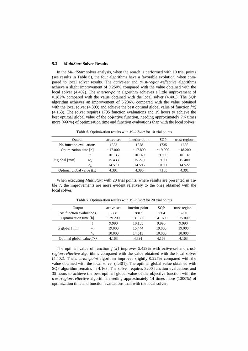
5.3 MultiStart Solver Results
In the MultiStart solver analysis, when the search is performed with 10 trial points
(see results in Table 6), the four algorithms have a favorable evolution, when com-
pared to local solver results. The active-set and trust-region-reflective algorithms
achieve a slight improvement of 0.250% compared with the value obtained with the
local solver (4.402). The interior-point algorithm achieves a little improvement of
0.182% compared with the value obtained with the local solver (4.401). The SQP
algorithm achieves an improvement of 5.236% compared with the value obtained
with the local solver (4.393) and achieve the best optimal global value of function f(x)
(4.163). The solver requires 1735 function evaluations and 19 hours to achieve the
best optimal global value of the objective function, needing approximately 7.6 times
more (660%) of optimization time and function evaluations than with the local solver.
Table 6. Optimization results with MultiStart for 10 trial points
Output active-set interior-point SQP trust-region-
Nr. function evaluations 1553 1628 1735 1665
Optimization time [h] ~17.000 ~17.800 ~19.000 ~18.200
x global [mm]
t 10.135 10.140 9.990 10.137
wa 15.433 15.279 19.000 15.400
hb 14.519 14.596 10.000 14.522
Optimal global value f(x) 4.391 4.393 4.163 4.391
When executing MultiStart with 20 trial points, where results are presented in Ta-
ble 7, the improvements are more evident relatively to the ones obtained with the
local solver.
Table 7. Optimization results with MultiStart for 20 trial points
Output active-set interior-point SQP trust-region-
Nr. function evaluations 3588 2887 3804 3200
Optimization time [h] ~39.200 ~31.500 ~41.600 ~35.000
x global [mm]
t 9.990 10.135 9.990 9.990
wa 19.000 15.444 19.000 19.000
hb 10.000 14.513 10.000 10.000
Optimal global value f(x) 4.163 4.391 4.163 4.163
The optimal value of function ( ) improves 5.429% with active-set and trust-
region-reflective algorithms compared with the value obtained with the local solver
(4.402). The interior-point algorithm improves slightly 0.227% compared with the
value obtained with the local solver (4.401). The optimal global value obtained with
SQP algorithm remains in 4.163. The solver requires 3200 function evaluations and
35 hours to achieve the best optimal global value of the objective function with the
trust-region-reflective algorithm, needing approximately 14 times more (1300%) of
optimization time and function evaluations than with the local solver.

5.4 Discussion of Results
Following the discussion of results is presented for local and global solutions.
Local Solution Discussion
In general, the local solver fmincon converges to a good solution for the four algo-
rithms, achieving a correlation of mode shapes and natural frequencies, between the
reference and numerical model, with good quality.
The color graphs of Fig.4 represent the MAC matrix and frequencies matrix, and
quantifies the correlation among the reference and numerical model. In matrix
the diagonal should be as dark as possible and bright outside of the diagonal, to repre-
sent a good correlation among mode shapes, and the frequencies matrix should be as
bright as possible to represent a good correlation among the frequencies.
Fig. 4. Initial correlation
The value of first function evaluation, for any used algorithms, is 23.042, because
the initial point is the same for all cases. This value has the meaning of the geo-
metric distance between the reference model and initial numerical model, imposed by
initial variables of point .This originates a weak correlation between, mainly, the
natural frequency values of the two models, since the correlation between all mode
shapes in diagonal MAC matrix is quite close to the unit, as shown in Fig.4.
After the optimization is complete, the quality of the natural frequencies correla-
tion improves considerably, and reveals a slight improvement in MAC matrix, as
shown in Fig.5a. The SQP algorithm is the one that achieves the best optimal value of
objective function, and consequently, the best correlation among the two models.
The final numerical model, presented in Fig.5b, suffers significant changes due to
the convergence of width (wa) and height (hb) parameters to the upper bounds. As the
thickness (t) parameter suffers a small change in relation to the initial value, the nu-
merical model is now closer to the reference model, both geometrically and in terms
of its dynamic behavior.
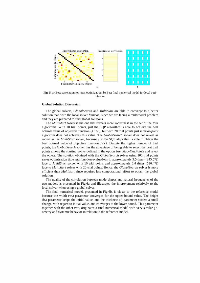
Fig. 5. a) Best correlation for local optimization; b) Best final numerical model for local opti-
mization
Global Solution Discussion
The global solvers, GlobalSearch and MultiStart are able to converge to a better
solution than with the local solver fmincon, since we are facing a multimodal problem
and they are prepared to find global solutions.
The MultiStart solver is the one that reveals more robustness in the set of the four
algorithms. With 10 trial points, just the SQP algorithm is able to achieve the best
optimal value of objective function (4.163), but with 20 trial points just interior-point
algorithm does not achieves this value. The GlobalSearch solver does not reveal as
robust as the MultiStart solver, because just the SQP algorithm is able to obtain the
best optimal value of objective function ( ). Despite the higher number of trial
points, the GlobalSearch solver has the advantage of being able to select the best trail
points among the starting points defined in the option NumStageOnePoints and reject
the others. The solution obtained with the GlobalSearch solver using 100 trial points
saves optimization time and function evaluations in approximately 3.5 times (245.5%)
face to MultiStart solver with 10 trial points and approximately 6.4 times (536.4%)
face to MultiStart solver with 20 trial points. Hence, the GlobalSearch solver is more
efficient than Multistart since requires less computational effort to obtain the global
solution.
The quality of the correlation between mode shapes and natural frequencies of the
two models is presented in Fig.6a and illustrates the improvement relatively to the
local solver when using a global solver.
The final numerical model, presented in Fig.6b, is closer to the reference model
because the width (wa) parameter converges for the upper bound value. The height
(hb) parameter keeps the initial value, and the thickness (t) parameter suffers a small
change, with regard to initial value, and converges to the lower bound. This parameter
together with the other two, originates a final numerical model with very similar ge-
ometry and dynamic behavior in relation to the reference model.

Fig. 6. a) Best correlation for global optimization; b) Best final numerical model for global
optimization
6 Conclusions
The aim of this paper was to apply two stochastic global optimization techniques
for the optimization of a dynamic structural finite element model, and to establish a
comparison with the previously local search method used in the Finite Element Model
Updating program. The global solvers have the advantage of being able to work with
a higher number of trial points, and therefore, are more efficient than the local solver.
The two global solvers tested work in a different way, and therefore the results may
also be different. Both global solvers achieve the same optimal global value of the
objective function, requiring, however, different optimization times and function
evaluations. In this case, the GlobalSearch is the fastest solver to achieve the best
optimal global value when working with the SQP algorithm. The MultiStart solver
achieved the same best optimal global value with the active-set, SQP and trust-
region-reflective algorithms however needed six times more computational effort in
terms of execution time and number of function evaluations.
The example used can be considered too oriented, which may increase the possibil-
ity of convergence of the local method, and somehow reduce the ability of perception
of higher capacity of global methods. However, it was evident the evolution of the
final numerical model to get closer to the geometry of the reference model when ap-
plied global optimization techniques.
In the future, more complex models will be studied and the use of stochastic global
optimization methods based on Swarm Intelligence will be investigated.
Acknowledgments. The authors gratefully acknowledge the Centre for Mechanical
and Materials Technologies (CT2M) and the Portuguese Funds through FCT -
"Fundação para a Ciência e a Tecnologia" under Project PEst-OE/EEI/UI0319/2014.

References
1. Nocedal, J., Wright, S. J.: Numerical Optimization. Series in Operations Research,
Springer Verlag, Heidelberg (1999)
2. Horst, R., Pardalos P.: Handbook of Global Optimization. Kluwer (1995)
3. Horst, R., Tuy, H.: Global Optimization Deterministic Approaches. Springer (1996)
4. Törn, A., Zilinskas, A.: Global Optimization. Springer-Verlag (1989)
5. Stolpe, M.: Global optimization of minimum weight truss topology problems with stress,
displacement, and local buckling constraints using branch-and-bound. Int. J. Numer. Meth.
Eng. 61, 1270–1309 (2004)
6. Achtziger, W., Stolpe M.: Truss topology optimization with discrete design variables -
Guaranteed global optimality and benchmark examples. Struct Multidisc Optim. 34, 1-20
(2007)
7. Lin, C.-Y., Chen W.-T.: Stochastic multistage algorithms for multimodal structural opti-
mization. Comp. Struct. 24, 233-241 (2000)
8. Lucor, D., Enaux, C., Jourdren, H., Sagaut, P.: Stochastic design optimization: Application
to reacting flows. Comput. Method Appl. M. 196, 5047-5062 (2007)
9. Birbil, S. I.: Stochastic Global Optimization Techniques, Faculty of North Carolina State
University of Raleigh (2002)
10. Eriksson, P., Arora, J. S.: A comparison of global optimization algorithms applied to a ride
comfort optimization problem. Struct. Multidisc. Optim. 24, 157–167 (2002)
11. Sonmez, F. O.: Shape optimization of 2D structures using simulated annealing. Comput.
Method Appl. M. 196, 3279-3299 (2007)
12. Venanzi, I., Materazzi, A. L.: Multi-objective optimization of wind-excited structures.
Eng. Struct. 23, 983-990 (2007)
13. Auvinen, P., Makela, M. M., Makinen, J.: Structural optimization of forest machines with
hybridized nonsmooth and global methods. Struct. Multidisc. Optim. 23, 382–389 (2002)
14. Keller, D.: Global laminate optimization on geometrically partitioned shell structures.
Struct Multidisc Optim., 43, 353–368 (2011)
15. Mottershead, J. E., Friswell, M. I.: Model updating in structural dynamics: A survey. J.
Sound Vib. 167, 347-375 (1993)
16. Maia, N., Montalvão e Silva, J.: Theoretical and Experimental Modal Analysis. Hertford-
shire: Research Studies Press Ltd (1997)
17. Levin, R., Lieven, N.: Dynamic Finite Element Model Updating Using Simulated Anneal-
ing and Genetic Algorithms, Mech. Syst. Signal Pr. 12, 91–120 (1998)
18. Teughels, A., De Roeck, G., Suykens, J. A. K.: Global Optimization by coupled local min-
imizers and its application to FE model updating. Comp. Struct. 81, 2337-2351 (2003)
19. Bakir, P. G., Reynders, E., De Roeck, G.: An improved finite element model updating
method by the global optimization technique ‘Coupled Local Minimizers’. Comp. Struct.
86, 1339-1352 (2008)
20. Ameri, E., Aghdam, M. M., Shakeri M.: Global optimization of laminated cylindrical pan-
els based on fundamental natural frequency. Compos. Struct. 94, 2697-2705 (2012)
21. Meireles J.: Análise Dinâmica de Estruturas por Modelos de Elementos Finitos Identifica-
dos Experimentalmente, PhD Thesis, University of Minho (in Portuguese) (2007)
22. Allemang, R. J., Brown, D. L.: A Correlation Coefficient for Modal Vector Analysis. In
Proceedings of the 1st International Modal Analysis Conference, Florida, Holiday Inn
(1982)
23. MathWorks, Global Optimization Toolbox: User’s Guide R2011b. Massachusetts: The
MathWorksInc (2011)

24. Voormeren, S., Rixen, R., Updating component reduction bases of static and vibration
modes using preconditioned iterative techniques. Comput. Method Appl. M. 253, 39-59
(2013)