a genetically-motivated heuristic for route discovery and selection … · a genetically-motivated...
TRANSCRIPT
A Genetically-Motivated Heuristic for Route Discovery and
Selection in Packet-Switched Networks
by
Peter T. Whiting
B.S.E.E. Brigham Young University, Provo UT 1991
M.S.E.E. Brigham Young University, Provo UT 1992
Submitted to the Department of Electrical Engineering and Computer Science
and the Faculty of the Graduate School of the University of Kansas in partial
fulfillment of the requirements for the degree of Doctor of Philosophy.
Chairman
Committee Members
Date dissertation defended

Acknowledgments
I appreciate the many people who have been influential in helping me complete
this research. In particular, I acknowledge the contribution and support of the
faculty of the University of Kansas. Many professors have helped me through-
out this process. In particular, my adviser, Joseph Evans, has been a constant
source of encouragement. His friendship and sense of humor has lessened the
sting of an otherwise painful process.
I would not have completed this dissertation without the support of my
employer, Sprint, which provided me with the time and means to return to
school. Kurt Gastrock has gone beyond encouragement, right up to the point
of threatening my job, to make sure I allocated sufficient time to this effort. I
am grateful for his support and never-ending enthusiasm.
My family has been central to every success in my life. I thank my parents
for teaching me the value of hard work, both physical and mental. I am grateful
to my older brother Eric. Not only did he suffer through this entire document
to provide comments and feedback, but he threatened physical harm if I did
not finish. Fear is a great motivator.
i

Natalie, my spouse and best friend, deserves more thanks than I can express
here. She has read this entire document multiple times, finding a deluge of
grammar and spelling errors, rewording sentences that were awkward, and
pointing out where things needed to be clarified. Perhaps more important, she
willingly accepted an increased portion of our shared domestic responsibilities
to provide me the time required to finish. She never complained (unless you
count the times she would tease me about being crazy for even starting). This
dissertation would never have been completed without her.
And finally, I thank my high school science teacher, Rollie Cox. Mr. Cox put
up with an ungrateful, rude, and self-absorbed teenager and somehow man-
aged to instill within me a love of science and and a thirst for knowledge. I
dedicate this work to him and all the other women and men who have devoted
their lives to teaching. It is often a thankless job, but it shapes the world.
ii

Abstract
Route discovery and selection are fundamental to packet-switched networks.
As a packet transits a network, routers determine the path on which the packet
will be forwarded. The primary objective of a routing system is to discover
feasible and efficient routes for packets to follow in the network.
Finding the minimum-delay route that does not exceed capacity constraints
is a difficult problem. Besides being inherently complex, the problem is intrin-
sically distributed with strong real-time constraints. In addition, the input to
the problem may be unrealistically large or simply unavailable. Therefore, the
input is often simplified and approximated, sometimes using broad and un-
realistic assumptions. Because these assumptions introduce error, solving the
routing problem precisely is of limited value. Heuristic approaches offer a po-
tential balance between accuracy and computational feasibility.
The purpose and contribution of this research is to evaluate both the ana-
lytical and empirical performance of an adaptive routing heuristic that bases
its operation on a genetic metaphor. The system simulates evolution, borrow-
ing from nature’s familiar operators of reproduction, mutation, and selection.
As the landscape changes, the system evolves with it. By modeling nature’s
iii

“survival of the fittest” optimization operator, near-optimal routing tables can
be cultured in the network “petri dish.” The proposed heuristic operates with-
out an explicit knowledge of the network’s topology or traffic characteristics.
As such, it is well suited to an environment where this information is unavail-
able or changing. In addition, the proposed heuristic is simple, both in concept
and implementation. This research demonstrates that the method is capable of
finding near-optimal routes in the topologies studied. Analysis is provided to
demonstrate that the behavior of the heuristic can be modeled and accurately
predicted.
The approach has limitations and shortcomings. However, like the genetic
mutations it seeks to model, this approach represents an evolutionary step in
routing protocol design. Hence, understanding its strengths and weaknesses is
essential to determine if, when, and how characteristics of the heuristic are to
be incorporated into future routing protocols. Developing this understanding
is the motivation for this research.
iv

Contents
1 Introduction 1
1.1 The Routing Problem . . . . . . . . . . . . . . . . . . . . . . . . . . 1
1.2 Contribution of This Research . . . . . . . . . . . . . . . . . . . . . 3
1.3 Organization . . . . . . . . . . . . . . . . . . . . . . . . . . . . . . . 5
2 Background 6
2.1 Network Model: Defining the Problem . . . . . . . . . . . . . . . . 6
2.1.1 Challenges in Defining the System Input . . . . . . . . . . 8
2.1.2 Challenges in Defining the Objective Function . . . . . . . 10
2.1.3 Challenges Related to Computational Complexity . . . . . 10
2.1.4 Problem Summary . . . . . . . . . . . . . . . . . . . . . . . 11
2.2 Related Research . . . . . . . . . . . . . . . . . . . . . . . . . . . . 12
2.2.1 Routing . . . . . . . . . . . . . . . . . . . . . . . . . . . . . 12
2.2.2 Algorithms Motivated by Natural Processes . . . . . . . . 19
2.2.3 Genetic Routing Algorithms . . . . . . . . . . . . . . . . . 21
2.3 Approach Proposed by this Work . . . . . . . . . . . . . . . . . . . 24
v
3 The Proposed Heuristic 26
3.1 Overview . . . . . . . . . . . . . . . . . . . . . . . . . . . . . . . . . 27
3.1.1 Parasites . . . . . . . . . . . . . . . . . . . . . . . . . . . . . 27
3.1.2 Populations . . . . . . . . . . . . . . . . . . . . . . . . . . . 28
3.1.3 Forwarding . . . . . . . . . . . . . . . . . . . . . . . . . . . 28
3.2 Operators and Parameters . . . . . . . . . . . . . . . . . . . . . . . 29
3.2.1 Initial Population . . . . . . . . . . . . . . . . . . . . . . . . 30
3.2.2 Population Control . . . . . . . . . . . . . . . . . . . . . . . 31
3.2.3 Selection . . . . . . . . . . . . . . . . . . . . . . . . . . . . . 33
3.2.4 Reproduction . . . . . . . . . . . . . . . . . . . . . . . . . . 34
3.2.5 Mutation . . . . . . . . . . . . . . . . . . . . . . . . . . . . . 37
3.2.6 Sampling . . . . . . . . . . . . . . . . . . . . . . . . . . . . 38
3.2.7 Summary of Operators and Parameters . . . . . . . . . . . 40
3.3 Congestion . . . . . . . . . . . . . . . . . . . . . . . . . . . . . . . . 42
3.3.1 Output Queue Overflow . . . . . . . . . . . . . . . . . . . 43
3.3.2 Random Early Detect . . . . . . . . . . . . . . . . . . . . . 44
3.4 Chapter Summary . . . . . . . . . . . . . . . . . . . . . . . . . . . . 46
4 Analysis of a Triplet Network 48
4.1 Triplet Network State Model . . . . . . . . . . . . . . . . . . . . . . 49
4.2 State Analysis of the Triplet Network . . . . . . . . . . . . . . . . . 50
4.3 Time to Converge . . . . . . . . . . . . . . . . . . . . . . . . . . . . 54
4.3.1 Counting Routing Errors Only . . . . . . . . . . . . . . . . 57
vi

4.4 Empirical Results . . . . . . . . . . . . . . . . . . . . . . . . . . . . 58
4.5 Understanding the Effects of the Parameters . . . . . . . . . . . . 60
4.5.1 Minimum Representation . . . . . . . . . . . . . . . . . . . 60
4.5.2 Maximum Population Size . . . . . . . . . . . . . . . . . . 61
4.5.3 Initial Population . . . . . . . . . . . . . . . . . . . . . . . . 61
4.5.4 Sample Rate . . . . . . . . . . . . . . . . . . . . . . . . . . . 62
4.6 Chapter Summary . . . . . . . . . . . . . . . . . . . . . . . . . . . . 62
5 Analysis of a Ring Network 64
5.1 Topology . . . . . . . . . . . . . . . . . . . . . . . . . . . . . . . . . 65
5.1.1 Defining the Shortest Path . . . . . . . . . . . . . . . . . . . 67
5.1.2 Expected Delay Analysis . . . . . . . . . . . . . . . . . . . 68
5.2 Simulation Results for a Static System . . . . . . . . . . . . . . . . 73
5.2.1 Measured Delay for Shortest-Path Routing . . . . . . . . . 73
5.2.2 Measured Delay for the Heuristic Approaches . . . . . . . 75
5.2.3 Delay Variance Between Packets . . . . . . . . . . . . . . . 78
5.2.4 Population Stability over Time . . . . . . . . . . . . . . . . 85
5.2.5 Solution Variance for the Delay-Agnostic Heuristic . . . . 88
5.2.6 Static Ring Topology Summary . . . . . . . . . . . . . . . . 91
5.3 Simulation Results for a Dynamically Changing Network . . . . . 91
5.3.1 The New Topology . . . . . . . . . . . . . . . . . . . . . . . 92
5.3.2 Understanding the Effect of Round-Trip Time . . . . . . . 95
5.3.3 Predicting the Effect of the RED operator . . . . . . . . . . 97
vii

5.3.4 Dynamic Ring Topology Summary . . . . . . . . . . . . . . 101
5.4 Chapter Summary . . . . . . . . . . . . . . . . . . . . . . . . . . . . 102
6 Analysis of a Regional Network 104
6.1 Topology . . . . . . . . . . . . . . . . . . . . . . . . . . . . . . . . . 105
6.2 Single-Flow Analysis . . . . . . . . . . . . . . . . . . . . . . . . . . 106
6.2.1 Small Flow . . . . . . . . . . . . . . . . . . . . . . . . . . . . 108
6.2.2 Medium Flow . . . . . . . . . . . . . . . . . . . . . . . . . . 111
6.2.3 Large Flow . . . . . . . . . . . . . . . . . . . . . . . . . . . 116
6.3 Multiple Flows . . . . . . . . . . . . . . . . . . . . . . . . . . . . . 119
6.3.1 Adding a Flow from fw→phx . . . . . . . . . . . . . . . . 119
6.3.2 Adding a Flow from pen→kc . . . . . . . . . . . . . . . . . 121
6.3.3 Adding a Flow from fw→phx and from pen→kc . . . . . 124
6.3.4 Adding a flow from atl→sj . . . . . . . . . . . . . . . . . . 126
6.4 All-Pairs Flows . . . . . . . . . . . . . . . . . . . . . . . . . . . . . 128
6.5 Chapter Summary . . . . . . . . . . . . . . . . . . . . . . . . . . . . 133
7 Challenges for the Heuristic 135
7.1 General Network-Related Challenges . . . . . . . . . . . . . . . . 136
7.1.1 Time-to-Live of Packets . . . . . . . . . . . . . . . . . . . . 136
7.1.2 High-Degree Nodes . . . . . . . . . . . . . . . . . . . . . . 139
7.1.3 Network Diameter . . . . . . . . . . . . . . . . . . . . . . . 140
7.1.4 Summary of Network-Related Challenges . . . . . . . . . 141
7.2 Challenges Specific to IP Networks . . . . . . . . . . . . . . . . . . 142
viii
7.2.1 Destinations . . . . . . . . . . . . . . . . . . . . . . . . . . . 142
7.2.2 Packet Reordering . . . . . . . . . . . . . . . . . . . . . . . 144
7.2.3 Multicast . . . . . . . . . . . . . . . . . . . . . . . . . . . . . 146
7.2.4 Fragmentation . . . . . . . . . . . . . . . . . . . . . . . . . 146
7.2.5 Space for Options in the Header . . . . . . . . . . . . . . . 147
7.2.6 BGP Interaction . . . . . . . . . . . . . . . . . . . . . . . . . 148
7.2.7 Summary of IP-Related Challenges . . . . . . . . . . . . . . 149
7.3 Chapter Summary . . . . . . . . . . . . . . . . . . . . . . . . . . . . 149
8 Implementation Considerations 151
8.1 Efficient Parasite Encodings . . . . . . . . . . . . . . . . . . . . . . 152
8.2 Timestamps and Global Clocks . . . . . . . . . . . . . . . . . . . . 154
8.3 Summary . . . . . . . . . . . . . . . . . . . . . . . . . . . . . . . . . 155
9 Conclusions 156
A Complexity of FLOW ASSIGNMENT 166
B Additional Ring Dynamics 168
B.1 Removing a Link from the Topology . . . . . . . . . . . . . . . . . 168
B.2 Changing Flow Size . . . . . . . . . . . . . . . . . . . . . . . . . . . 171
B.2.1 Change in Available Path Capacity . . . . . . . . . . . . . . 172
B.3 Summary . . . . . . . . . . . . . . . . . . . . . . . . . . . . . . . . . 174
ix

List of Figures
3.1 Roulette wheel selection operator . . . . . . . . . . . . . . . . . . . 33
4.1 Triplet network topology . . . . . . . . . . . . . . . . . . . . . . . . 49
4.2 State space for a router with two links . . . . . . . . . . . . . . . . 51
4.3 State transitions for a router with two links . . . . . . . . . . . . . 52
4.4 State transitions for node 2 in the triplet network . . . . . . . . . . 53
4.5 The acceptable region of the state space . . . . . . . . . . . . . . . 53
4.6 State transitions for node 2 in the triplet network when y = ηmin . 55
4.7 State transitions for node 2 in the triplet network when x+y = ψmax 56
5.1 Ring network topology . . . . . . . . . . . . . . . . . . . . . . . . . 65
5.2 Delay surface for routing in the ring network . . . . . . . . . . . . 71
5.3 Measured vs. calculated delay for shortest-path approach using
the low-delay path . . . . . . . . . . . . . . . . . . . . . . . . . . . 74
5.4 Measured vs. calculated delay for shortest-path approach using
the high-capacity path . . . . . . . . . . . . . . . . . . . . . . . . . 74
5.5 Measured vs. calculated delay for shortest-path approach using
both paths equally . . . . . . . . . . . . . . . . . . . . . . . . . . . 75
x
5.6 Delay vs. load plot for both heuristic methods . . . . . . . . . . . 76
5.7 Combined delay vs. load plots for the ring network . . . . . . . . 77
5.8 Sampled packet delay for a 15 Mb/s flow using the shortest-path
approach routing all traffic on the low-delay path . . . . . . . . . 79
5.9 Sampled packet delay for a 15 Mb/s flow using the shortest-path
approach routing traffic on the high-capacity path . . . . . . . . . 79
5.10 Sampled packet delay for a 15 Mb/s flow using the shortest-path
approach routing traffic on both paths equally . . . . . . . . . . . 80
5.11 Packet delay for a 15 Mb/s flow using the delay-agnostic heuristic 80
5.12 Packet delay for a 15 Mb/s flow using the delay-aware heuristic . 81
5.13 Tukey boxplots for all approaches with 5 Mb/s flows . . . . . . . 82
5.14 Tukey boxplots for all approaches with 15 Mb/s flows . . . . . . . 83
5.15 Tukey boxplots for all approaches with 25 Mb/s flows . . . . . . . 83
5.16 Tukey boxplots for all approaches with 35 Mb/s flows . . . . . . . 84
5.17 Percent of population favoring link toward node 1 for 5 Mb/s flow 86
5.18 Percent of population favoring link toward node 1 for 15 Mb/s
flow . . . . . . . . . . . . . . . . . . . . . . . . . . . . . . . . . . . . 86
5.19 Percent of population favoring link toward node 1 for 25 Mb/s
flow . . . . . . . . . . . . . . . . . . . . . . . . . . . . . . . . . . . . 87
5.20 Percent of population favoring link toward node 1 for 35 Mb/s
flow . . . . . . . . . . . . . . . . . . . . . . . . . . . . . . . . . . . . 87
5.21 Percent of population favoring link toward node 1 for 39 Mb/s
flow . . . . . . . . . . . . . . . . . . . . . . . . . . . . . . . . . . . . 88
xi

5.22 Histogram for 100 runs of delay-agnostic heuristic with 5 Mb/s
flows . . . . . . . . . . . . . . . . . . . . . . . . . . . . . . . . . . . 89
5.23 Histogram for 100 runs of delay-agnostic heuristic with 15 Mb/s
flows . . . . . . . . . . . . . . . . . . . . . . . . . . . . . . . . . . . 90
5.24 Histogram for 100 runs of delay-agnostic heuristic with 25 Mb/s
flows . . . . . . . . . . . . . . . . . . . . . . . . . . . . . . . . . . . 90
5.25 Histogram for 100 runs of delay-agnostic heuristic with 35 Mb/s
flows . . . . . . . . . . . . . . . . . . . . . . . . . . . . . . . . . . . 91
5.26 Ring topology with added link . . . . . . . . . . . . . . . . . . . . 93
5.27 Portion of population on node 0 favoring link toward node 1,
delay-aware and delay-agnostic . . . . . . . . . . . . . . . . . . . . 94
5.28 Portion of population on node 1 favoring link toward node 4,
predicted and measured . . . . . . . . . . . . . . . . . . . . . . . . 101
5.29 Portion of population on node 0 favoring link toward node 1,
predicted and measured . . . . . . . . . . . . . . . . . . . . . . . . 102
6.1 Instance of a regional network topology . . . . . . . . . . . . . . . 106
6.2 Average delay for 10 Mb/s nyc→phx flow . . . . . . . . . . . . . . 109
6.3 Average delay for 25 Mb/s nyc→phx flow . . . . . . . . . . . . . . 114
6.4 Average delay for 75 Mb/s nyc→phx flow . . . . . . . . . . . . . . 116
6.5 Packet loss for 75 Mb/s nyc→phx flow . . . . . . . . . . . . . . . . 117
6.6 Average delay for 25 Mb/s nyc→phx flow and 10 Mb/s fw→phx
flow . . . . . . . . . . . . . . . . . . . . . . . . . . . . . . . . . . . . 120
xii

6.7 Packet loss for 25 Mb/s nyc→phx flow and 10 Mb/s fw→phx flow121
6.8 Average delay for 25 Mb/s nyc→phx flow and 10 Mb/s pen→kc
flow . . . . . . . . . . . . . . . . . . . . . . . . . . . . . . . . . . . . 122
6.9 Packet loss for 25 Mb/s nyc→phx flow and 10 Mb/s pen→kc flow 123
6.10 Average delay for 25 Mb/s nyc→phx flow, 10 Mb/s pen→kc flow,
and 10 Mb/s fw→phx flow . . . . . . . . . . . . . . . . . . . . . . 125
6.11 Packet loss for 25 Mb/s nyc→phx flow, 10 Mb/s pen→kc flow,
and 10 Mb/s fw→phx flow . . . . . . . . . . . . . . . . . . . . . . 125
6.12 Average delay for 25 Mb/s nyc→phx flow and 40 Mb/s pen→kc
flow . . . . . . . . . . . . . . . . . . . . . . . . . . . . . . . . . . . . 127
6.13 Packet loss for 25 Mb/s nyc→phx flow and 40 Mb/s pen→kc flow 128
6.14 Average delay for flows between every pair of nodes in the net-
work . . . . . . . . . . . . . . . . . . . . . . . . . . . . . . . . . . . 129
6.15 Packet loss for flows between every pair of nodes in the network 130
6.16 Average delay for flows between every pair of nodes in the net-
work with 50% traffic increase . . . . . . . . . . . . . . . . . . . . . 132
6.17 Packet loss for flows between every pair of nodes in the network
with 50% traffic increase . . . . . . . . . . . . . . . . . . . . . . . . 132
A.1 Transformation from PARTITION to FLOW ASSIGNMENT . . . 167
B.1 Ring topology with link removed . . . . . . . . . . . . . . . . . . . 170
B.2 Probability of node 0 sending traffic toward node 1 before and
after a link is removed . . . . . . . . . . . . . . . . . . . . . . . . . 170
xiii

B.3 PDF for changing flow at 5 Mb/s . . . . . . . . . . . . . . . . . . . 172
B.4 PDF for changing flow at 15 Mb/s . . . . . . . . . . . . . . . . . . 173
B.5 PDF for changing flow at 15 Mb/s . . . . . . . . . . . . . . . . . . 174
xiv

List of Tables
3.1 Parameter values used in this research . . . . . . . . . . . . . . . . 42
6.1 Regional network delay matrix (in ms) . . . . . . . . . . . . . . . . 107
6.2 Regional network capacity matrix (in Mb/s) . . . . . . . . . . . . 107
6.3 Packet loss for 10 Mb/s nyc→phx flow . . . . . . . . . . . . . . . . 109
6.4 Packet loss for 25 Mb/s nyc→phx flow . . . . . . . . . . . . . . . . 115
6.5 Average delay for 75 Mb/s nyc→phx flow . . . . . . . . . . . . . . 117
6.6 Packet loss for 75 Mb/s nyc→phx flow . . . . . . . . . . . . . . . . 117
6.7 Average delay for 25 Mb/s nyc→phx flow and 10 Mb/s fw→phx
flow . . . . . . . . . . . . . . . . . . . . . . . . . . . . . . . . . . . . 120
6.8 Packet loss for 25 Mb/s nyc→phx flow and 10 Mb/s fw→phx flow120
6.9 Average delay for 25 Mb/s nyc→phx flow and 10 Mb/s pen→kc
flow . . . . . . . . . . . . . . . . . . . . . . . . . . . . . . . . . . . . 123
6.10 Packet loss for 25 Mb/s nyc→phx flow and 10 Mb/s pen→kc flow 123
6.11 Average delay for 25 Mb/s nyc→phx flow, 10 Mb/s pen→kc flow,
and 10 Mb/s fw→phx flow . . . . . . . . . . . . . . . . . . . . . . 124
xv
6.12 Packet loss for 25 Mb/s nyc→phx flow, 10 Mb/s pen→kc flow,
and 10 Mb/s fw→phx flow . . . . . . . . . . . . . . . . . . . . . . 126
6.13 Average delay for 25 Mb/s nyc→phx flow and 40 Mb/s pen→kc
flow . . . . . . . . . . . . . . . . . . . . . . . . . . . . . . . . . . . . 127
6.14 Packet loss for 25 Mb/s nyc→phx flow and 40 Mb/s pen→kc flow 127
6.15 Average delay for flows between every pair of nodes in the net-
work . . . . . . . . . . . . . . . . . . . . . . . . . . . . . . . . . . . 129
6.16 Packet loss for flows between every pair of nodes in the network 130
6.17 Average delay for flows between every pair of nodes in the net-
work with 50% traffic increase . . . . . . . . . . . . . . . . . . . . . 131
6.18 Packet loss for flows between every pair of nodes in the network
with 50% traffic increase . . . . . . . . . . . . . . . . . . . . . . . . 133
6.19 Summarization of the performance across all experiments . . . . 134
xvi
Chapter 1
Introduction
The task of discovering and selecting routes is fundamental to the operation
of packet-switched networks. Routers coordinate the path every packet takes
as it transits the network. To do this, routers need a consistent view of how
the packet is to proceed; otherwise a packet may be caught in a never-ending
loop. In addition to being consistent, the selected route should be efficient.
While the definition of efficiency is context-specific, generally it is beneficial
to minimize the total delay experienced by each packet in the network. The
primary objective of a routing system is to support the discovery and selection
of feasible and efficient routes.
1.1 The Routing Problem
Real-world networks have capacity constraints, and finding a path with min-
imum delay while not exceeding capacity is a difficult problem. Depending
on the objective function and topology the optimization problem may be NP-
1
complete. There are at least four significant characteristics of the routing prob-
lem that make it difficult to solve[13]:
• It is intrinsically distributed.
• It is stochastic and time-varying.
• It has multiple objectives that often conflict.
• It has multiple constraints.
In addition to these challenges, the input to the problem may be enormous in
size or even unavailable. Given these limitations, it is common to use approxi-
mations and heuristics in the pursuit of feasible and efficient routing solutions.
Routing protocols may be broadly classified as either static or adaptive.
Static protocols route traffic based entirely on packet destinations, oblivious to
network state. Their performance tends to be stable and deterministic. How-
ever, due to the intrinsic dynamics present in most real-world networks, the
inability of static protocols to adapt as the network and traffic characteristics
change is a major drawback. Adaptive protocols incorporate network state
into their routing decisions, and in theory offer the best hope for efficient use of
network resources. However, adaptive protocols frequently suffer from oscil-
latory behavior, as the feedback mechanisms operate on a time-scale that lags
the dynamics of both the network and traffic.
Early experience with adaptive routing in the ARPANET [59][47] demon-
strated the difficulty of developing a stable adaptive routing protocol. The re-
sult of this experience was the adoption of a class of routing protocols that,
2

although adaptive, only change based on the binary up/down state of each
link in the network[65][45], or, in other words, only adapt to the topology of
the network and not in response to real-time traffic characteristics. The task
of altering routing to accommodate changing traffic patterns was relegated to
network operators who manually adjust routing metrics.
While this approach has proven to be a stable and sustainable methodology
for managing large networks, it often distributes traffic suboptimally. Because
it is based on a manual process for selecting and updating metrics, it is difficult
for the system to adapt on the time-scale in which the traffic patterns are chang-
ing. In addition, this approach is incapable of non-uniformly distributing traffic
across multiple paths. Paths with equivalent cost may take equal portions of
the traffic, but there is no facility for one path to be assigned a larger percentage
of the traffic than another. When path capacities are asymmetric the flexibility
to distribute traffic non-uniformly is required for optimal traffic distribution.
This is referred to as non-minimal routing. Because of its inability to adapt
and its inability to distribute traffic non-uniformly, the current approach often
makes inefficient use of available network resources.
1.2 Contribution of This Research
The purpose of this research is to evaluate both analytically and empirically
the behavior of an adaptive routing methodology that bases its operation on
a genetic metaphor. Initially packets are routed randomly, but over time the
3
network of routers collects feedback regarding the feasibility of different paths.
The feedback model simulates evolution, borrowing from nature’s familiar op-
erators of reproduction, mutation, and selection. This research demonstrates
that, for the limited set of network topologies studied and with the traffic mod-
els employed, this simple feedback mechanism is able to produce favorable
results relative to those obtained using shortest-path routing techniques.
The approach evaluated in this dissertation diverges significantly from cur-
rent trends in routing protocol design that seek to offer more control and pro-
vide more information to the routing protocol. Many earlier applications of
genetically-motivated heuristics also work with similar control-plane assump-
tions. Such methods suffer when accurate traffic data is not available. This
work explores an approach that moves in the opposite direction: toward less
control. In fact, the routing technique described by this paper does not seek
to discover the network’s topology, does not require the setting of link metrics,
and does not require a priori knowledge of the anticipated traffic matrix. Rather,
each network node independently seeks to discover, based on feedback, opti-
mal egress links for aggregates of destination addresses. The process is contin-
uous, allowing routing to adapt and evolve as both the network topology and
the traffic characteristics change. Because the routers are not maintaining topo-
logical state, distributing new topology information in response to topological
changes is not required.
4

1.3 Organization
This document is structured as follows: Chapter 2 explores the background of
the routing problem. Included in this chapter is a summary of past and present
approaches to solving the routing problem. The chapter concludes with an
overview of other problems being addressed by genetic heuristics. Chapter 3
describes the heuristic approach proposed by this paper and defines many of
its operators and parameters. Chapter 4 analyzes the heuristic’s behavior on a
triplet network and quantifies the impact of some of the parameters described
in Chapter 3. Chapter 5 provides an analysis of the proposed heuristic on a spe-
cific instance of a ring network. Its performance is contrasted with what might
be expected from shortest-path routing systems. Consideration is given to the
algorithm’s ability to converge and adapt in both static and dynamic environ-
ments. Chapter 6 explores the performance of the heuristic on a more realistic
topology, one modeled after a regional network. This network is analyzed with
both simple and complex flow sets. As expected, the heuristic has limitations
and shortcomings, some of which are identified in Chapter 7. This chapter also
discusses possible mitigation techniques for these challenges. Chapter 9 sum-
marizes the research and provides conclusions.
5
Chapter 2
Background
The purpose of this chapter is to provide the reader with an understanding of
the routing problem and the challenges associated with solving it. Background
is provided on previous work done in this field, with an emphasis on the ex-
perience gained on the Internet’s predecessor, the ARPANET. In addition, this
chapter provides foundational theory for genetic algorithms, including exam-
ples of their application to the routing problem.
2.1 Network Model: Defining the Problem
A communications network may be modeled as a directed graph, G = (V,E),
where the set of nodes V represents the routers in the network and the set of
edges E represents communications links connecting the routers. Each edge, e,
in E has a capacity, c(e), and a delay, d(e).
c(e) = <+ ∀e ∈ E
d(e) = <+ ∀e ∈ E
6

The edges are unidirectional in order to accommodate asymmetries. Com-
munications links with symmetric bandwidth and delay are drawn as single
bi-directional edges in order to simplify drawing network topologies.
The capacity of edge eij represents how many data units can be carried from
vi to vj . For a communications link modeled as a bit-pipe, the capacity is ex-
pressed in bits per second and is referred to as the link’s bandwidth.
The delay experienced by a packet transiting a communications link is com-
prised of at least four separate components:
1. Processing delay is the time between when a packet is received by a router
and when it is placed on an output queue. Among other things, this delay
is a function of the processor clock rate, route-lookup algorithm, size of
the routing table, and backplane scheduling algorithm.
2. Queueing delay is the amount of time the packet waits in queue for trans-
mission. It is a function of the packet inter-arrival times, the packet-size
distribution, and the capacity of the communications link.
3. Transmission delay is the time between when the first and last bits of the
packet are transmitted and is a function of the link’s bandwidth and the
packet size.
4. Propagation delay is the time it takes a single bit to travel from one end of
the communications link to the other. For all practical purposes this delay
is constant, and is the physical path distance divided by the speed of light
in fiber.
7

The delay of edge eij represents only the propagation delay between nodes vi
and vj . This research considers the processing delay to be negligible compared
to the propagation delay, an assumption that can be safely made for wide-area
network circuits. Queuing and transmission delays are combined in the queu-
ing delay analysis.
2.1.1 Challenges in Defining the System Input
Discrete groupings of bits are referred to as packets. Among other things,
each packet has associated with it a source and destination, defining where
the packet originated and where it is ultimately destined. For the purpose of
this work, both the source and the destination will be considered to be in the set
V . Discussion of how the model can accommodate networks providing transit
services where neither the source nor the destination are in the set V is pro-
vided in Section 7.2.1. In addition to the time-varying network topology, the
input to the routing problem includes the set of all packets to be introduced
into the network, their sizes, and the time each is created.
Large-scale networks might service many millions of packets each second.
Modeling each packet individually in such an environment would likely re-
sult in an unmanageably large data set. In addition to being too large, such
precise foreknowledge is rarely available. A common strategy for simplifying
the traffic data is to aggregate groups of packets traveling between common
source-destination pairs into flows. The flows are often defined using stochas-
8

tic models for packet size and inter-arrival time distributions. The choice of
models greatly affects whether the resultant problem will be tractable.
This research assumes exponentially distributed packet sizes and a Poisson
arrival process. The validity of arrival process assumption for Internet traffic
is both challenged and supported in the academic community[53][70][10][11].
The decision to use this arrival process was based on the desire to choose a
model for which the queuing theory is well understood. The validity of the
packet-size distribution is also questionable, as Internet traffic adheres to a tri-
modal packet-size distribution resulting from the maximum transmission unit
(MTU) of typical networks combined with TCP’s minimally-sized packets[19].
Again, the decision to use an exponential distribution was based on the desire
to fit into well-understood queuing models. In addition, although the Internet
is the focal point of much current research, this work is addresses the general
problem of packet switching, and not the specific problem of packet-switching
on today’s Internet.
Using the concept of flows, the above assumptions, and queuing theory es-
tablished over the past decades[49], meaningful analytic results may be ob-
tained for simple network topologies. To use this output to gauge the success
of a routing algorithm, one also must quantify success in terms of an objective
function.
9

2.1.2 Challenges in Defining the Objective Function
One of the challenges to arriving at a precise and relevant solution for the rout-
ing problem is defining a suitable objective function. An objective function
defines the goal of an optimization problem. The definition of the objective
function for the routing problem is context specific and subjective. Typically
there are multiple, sometimes conflicting, objectives. The focus of this work
is on two objectives: avoiding packet loss and minimizing delay. In general,
avoiding packet loss takes priority over minimizing delay. However, focusing
first on avoiding loss by minimizing link utilization without consideration of
the delay implications may result in a suboptimal solution. For example, con-
sider two links with equivalent bandwidth but vastly different delay. To min-
imize the loss probability the traffic should be distributed evenly between the
two links. However, if the amount of traffic is small compared to the available
bandwidth, a solution that routes more traffic over the link having lower delay
is preferable. The formulation of a strategy for determining how to quantify a
solution’s fitness is often subjective.
2.1.3 Challenges Related to Computational Complexity
The size of the input associated with route optimization on a per-packet basis is
often untenable. In order to decrease the size of the input, packets having com-
mon source and destination addresses are often grouped together into what
are referred to as flows. A flow typically has a stochastic model associated
with it defining both the arrival process and the packet-size distribution. Al-
10
though this simplifies the input, the computational complexity may be daunt-
ing, even for a simple objective function. Without the ability to divide (deag-
gregate) flows arbitrarily, the flow-assignment problem is NP-hard, even for an
objective function that ignores delay and only seeks to ensure that packets are
not lost. The proof for this is presented in Appendix A.
The flow-assignment problem would likely be more difficult if the objective
function combined multiple objectives. Joint optimization problems are often
NP-complete, and it has been shown that the problem of finding a path subject
to any two of the following metrics is NP-complete: delay, loss probability, cost,
and jitter[83]. While this same paper presents a solution for minimizing delay
with bandwidth constraints, it does not propose a solution that works for more
than a single flow.
2.1.4 Problem Summary
The computational complexity associated with finding a solution to the rout-
ing problem is significant. The definition of the objective function might be
imprecise and subjective. The input to the problem may be enormous. Perhaps
most significant, the input to the problem may not be available. These realities
must be considered when formulating an optimization approach. Rigorously
solving an imprecise problem with imprecise input may provide little advan-
tage over a more efficient heuristic approach. Such an approach is the focus
of this work. The remainder of this chapter will examine some of the previous
research related to solving the routing problem, including heuristic methods.
11

2.2 Related Research
As a result of the success of the Internet, interest in the routing problem has
increased significantly. During the same time-frame computational power has
increased dramatically. Genetic algorithms, once thought computationally in-
feasible, are now gaining mainstream acceptance as viable heuristic approaches
to complex problems. Given the complexity of the routing problem, it is not
surprising that genetic routing algorithms, routing techniques that model nat-
ural processes, are increasingly popular. This section begins with an overview
of previous work on the routing problem, followed by foundational theory for
genetic algorithms. This section concludes with a discussion of some of the
ongoing work in genetic routing algorithms.
2.2.1 Routing
Routing may be broadly classified in many ways: adaptive and non-adaptive,
minimal and non-minimal, central and distributed. This section includes an
overview of some of the early lessons learned on the Internet’s predecessor, the
ARPANET. This is followed by a discussion of current trends for routing on the
Internet.
Adaptive Routing
Adaptive routing may be defined as a routing system that adapts to the state of
the network. In some sense, most routing algorithms are minimally adaptive as
12
they take into account the topology of the network. However, the connotation
of adaptive routing is traditionally more broad, encompassing the idea of also
adjusting routing based on link utilization and other time-varying characteris-
tics related to network traffic. These techniques are typically reactive, and as
such may be subject to oscillatory behavior.
Early Lessons on the ARPANET
Early in the existence of the ARPANET, researchers tried several adaptive rout-
ing algorithms. The original ARPANET routing algorithm attempted to route
packets along paths of least delay by using a distributed version of the Bellman-
Ford shortest-path algorithm[4][36]. Each node would build a shortest-delay
routing table by estimating its delay to each of its adjacent nodes and then com-
bine these estimates with the routing tables received from each of its neighbors.
Each node would periodically send its updated table to all adjacent nodes. The
delay to a neighbor was estimated by simply counting the number of packets
in queue and then adding a constant value to account for propagation delay.
This technique did not work well for many reasons[71][58][59]. Among other
things, the delay estimate was found to be especially problematic. The effect
was instability and oscillations under heavy load. Hence, a new approach was
needed.
Researchers introduced a new routing protocol in May 1979 which sought to
correct the mistakes of the original ARPANET routing protocol[58][59]. One of
the more significant changes replaced the Bellman-Ford approach for shortest-
13
path calculation with a link-state approach. In the new approach each node in
the network maintained a database describing the complete network topology
and associated delays. Using this information each node could independently
build a shortest-path tree using Dijkstra’s shortest-path algorithm[25]. Because
of its search rule, this algorithm is frequently referred to as the shortest-path-
first (SPF) algorithm.
Two important considerations of the new approach were how to estimate
the delay and how to distribute the link-state information. Expected delay
was obtained from the measured average packet-delay in the system over a
10-second interval. The information was distributed through the network us-
ing a technique that later became known as reliable flooding. Reliable flooding
operates by having every node send its own link-state packets (LSPs) to each of
its neighbors. A node that receives an LSP floods it to all of its neighbors, except
the neighbor from which it received the LSP. Loops are avoided by assigning
a unique identifier to each LSP and ensuring that no router will re-forward an
LSP it has already seen. Reliable flooding ensures that every router eventually
obtains a consistent view of the topology. Transient routing loops exist dur-
ing periods when the routers have inconsistent views, but these are short and
infrequent.
Although this new approach represented a significant improvement, like its
predecessor, it tended to break down under heavy load[46][71]. During these
times the predictive accuracy of the measured delays decreased sharply, re-
sulting in poor correlation between the delay estimates and the actual delay
14

experienced after routing updates. This shortcoming, combined with the large
dynamic range of the metrics representing delay, resulted in large-scale traf-
fic oscillations. The effect of these oscillations was that a significant portion of
the network bandwidth would be idle while another portion of the network
would be over-used. In effect, the traffic would slosh back and forth between
links resulting in suboptimal performance.
The ARPANET’s final adaptive routing approach was termed “the revised
ARPANET routing metric”[46][71] and only replaced the metric calculation
logic of the previous system. This approach compressed the dynamic range
of the metrics and dampened the rate at which the advertised metric could
change. The new approach had the following characteristics[71]:
• A highly loaded link could cost no more than 3 times its lightly loaded
cost.
• The most expensive link (highly loaded 9.6 Kbs satellite link) could cost
no more than 7 times as much as the least expensive (lightly loaded 56 Kbs
terrestrial link).
• Terrestrial links were favored over satellite links having the same band-
width and utilization.
• High-speed satellite links were favored over low-speed terrestrial links.
• The cost was a function of utilization only at high loads.
The slopes, offsets, and breakpoints for the above parameters were determined
by trial and error.
15
The approach was effective for dealing with the oscillations but, in the long
run, did not scale with the rapidly expanding Internet. As newer, higher ca-
pacity circuits became available the parameters were not modified, and it soon
became obsolete.
EIGRP
Despite the challenges encountered in the early ARPANET experience, inter-
est in adaptive routing algorithms has continued. One notable commercially
developed protocol is Extended Inter-Gateway Routing Protocol (EIGRP)[2].
EIGRP uses the Diffusing Update Algorithm (DUAL)[39] for its shortest-path
computation. Like its predecessor, IGRP[43], EIGRP was designed to address
the limitations of Routing Information Protocol (RIP)[55]. Both RIP and EIGRP
are distance-vector protocols, but unlike RIP, EIGRP supports a wide range of
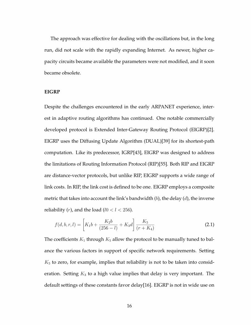
link costs. In RIP, the link cost is defined to be one. EIGRP employs a composite
metric that takes into account the link’s bandwidth (b), the delay (d), the inverse
reliability (r), and the load (l0 < l < 256).
f(d, b, r, l) =
[K1b+
K2b
(256− l)+K3d
]K5
(r +K4)(2.1)
The coefficients K1 through K5 allow the protocol to be manually tuned to bal-
ance the various factors in support of specific network requirements. Setting
K5 to zero, for example, implies that reliability is not to be taken into consid-
eration. Setting K3 to a high value implies that delay is very important. The
default settings of these constants favor delay[16]. EIGRP is not in wide use on
16
the core Internet routers today, possibly because of its proprietary nature which
conflicts with the open nature of the Internet.
Current Approach to Routing in the Internet
Despite the inherent advantages of adaptive routing, most current routing pro-
tocols are only minimally adaptive, adapting only when the topology of the
network changes. Link costs (metrics) are statically set and do not change
automatically in response to link utilization. Commonly used routing pro-
tocols include intermediate-system to intermediate-system (IS-IS)[9][45] and
open shortest path first (OSPF)[63][64][65]. These approaches are relatively
simple to implement and computationally efficient, as the shortest-path prob-
lem can be solved in O(V logV + E) time using Dijkstra’s algorithm[25] and
Fibonacci heaps[20].
These protocols are minimal routing techniques: they lack the ability to dis-
tribute traffic non-uniformly across multiple equal-cost paths. This limitation
not only affects the protocol’s ability to efficiently distribute traffic across multi-
ple paths with varied capacity, but it also affects the computational complexity
associated with determining an optimal assignment. This problem has been
shown to be NP-hard[37]. Due to the complexity of finding optimal assign-
ments for the metrics, they are often set using an ad-hoc methodology. Cisco
recommends setting metrics inversely proportional to link capacities[17]. This
approach has been shown to be non-optimal by [37] but is among the better
traffic-oblivious approaches. One approach would be to use this metric as a
17

starting point and then iteratively adjust the metric in response to traffic charac-
teristics using a manual trial-and-error process. More sophisticated approaches
include flow information in their calculations. This has potential benefits but,
as described previously, the input traffic matrix is typically only a rough ap-
proximation. Further complicating this problem for transit networks is the fact
that the input to the problem, the flows, may be affected by the output of the
algorithm, the metrics. For example, Border Gateway Protocol (BGP) uses the
internal metric as part of its decision function[77], and as such the egress router
selection is influenced by the internal metrics. Not only is the problem diffi-
cult to solve, it needs to be solved repeatedly, each time there is a significant
shift in traffic or topology. These factors combine to make the task of manually
managing the network a difficult and risky task.
MPLS
Multiprotocol Label Switching, or MPLS[30], is an encapsulation and forward-
ing mechanism designed to provide increased control of traffic within an IP
network. Originally, MPLS derived from earlier proposals focused on increas-
ing forwarding performance[68][18]. However, as processing power increased
this provided little value and the focus of MPLS shifted to traffic engineering.
MPLS found its first real application as a traffic-engineering tool[84] with
the introduction of signaling protocols such as LDP[29], RSVP-TE[54], and CR-
LDP[31]. Explicit routing is central to MPLS’s traffic-engineering capabilities.
Using explicit routing, MPLS can forward sub-aggregates of flows along paths
18
that do not necessarily follow ordinary IP routing rules. As such, MPLS offers
the ability to distribute traffic non-uniformly across multiple paths. In practice,
MPLS traffic engineering is most frequently used to direct traffic around under-
provisioned parts of a network.
Although MPLS may be used to distribute traffic non-uniformly across mul-
tiple paths, it still shares the problem of requiring an accurate estimate of the
traffic to be routed. In fact, its increased control capabilities may require more
detailed input data.
The approach proposed in this work is a step in the opposite direction. Not
only does the heuristic not require a knowledge of what the traffic distribution
will be, it does not even maintain a knowledge of the topology. While this may
seem counter-intuitive, the proposed heuristic will be shown to be a capable
methodology for routing traffic.
Logical thinking is unquestionably useful for many purposes. It usually
plays an important role in setting the stage for an invention. But, at the end
of the day, logical thinking is the antithesis of invention and creativity[52].
2.2.2 Algorithms Motivated by Natural Processes
The underlying metaphor of genetic algorithms is that of natural evolution.
In evolution, the problem each species faces is one of searching for
beneficial adaptations to a complicated and changing environment.
The ‘knowledge’ that each species has gained is embodied in the makeup
of the chromosomes of its members[21].
19

Research in genetic and evolutionary algorithms has been going on for over
forty years. Three works are generally recognized as foundational for the field:
• John Holland’s Adaptation in Natural and Artificial Systems[44].
• Ingo Rechenberg’s Evolutionstrategie: Optimierung Technisher Systeme nach
Prinzipien des Biologischen Evolution[76].
• Lawrence Fogel’s Artificial Intelligence through Simulated Evolution[35].
For the first three decades the field of genetic algorithms languished. Re-
searchers assumed the techniques could not be used to solve even the simplest
of problems[34]. However, the techniques may not have been as much at fault
as the limited computing power of the time. As computing power has increased
so has the ability to simulate the processes of evolution.
Genetic algorithms have the following basic components[21]:
• a means of encoding solutions to the problem as chromosomes,
• a means of obtaining an initial population of solutions,
• a function that evaluates the “fitness” of a solution,
• reproduction operators for the encoded solutions, and
• appropriate settings for the genetic algorithm control parameters.
These components are used iteratively to allow the population to evolve and
adapt over time.
20

2.2.3 Genetic Routing Algorithms
Due to their flexibility, especially when the actual problem is hard to state, ge-
netic and evolutionary algorithms have been employed in a broad range of
applications including supply-chain optimization [81], petroleum pricing[3],
nonlinear controllers for backing up a truck and trailer[15], and military target
recognition[82]. Even more extreme is the concept of genetic programming,
where computer programs are caused to evolve[51][6][52][74][75].
Genetic algorithms are also being applied to the routing problem[1][78][62].
An approach to discovering the two shortest node-disjoint paths between a pair
of routers has been described[1]. The use of agent-based genetic algorithms
in which agents are sent out on a network with one or more span failures to
discover a recovery path has been demonstrated[78]. Perhaps two of the better
known applications of genetic methods to routing are GBR[67] and AntNet[26].
GBR
The Genetic-Based Routing algorithm (GBR)[67][66] seeks to minimize hop
count and delay. In its initial stages, GBR operates much like existing link-state
algorithms, gathering topology information and identifying least-cost paths.
The algorithm uses unit cost for link cost, resulting in a hop-count-optimized
shortest-path topology.
GBR is a source-routed algorithm, completely pre-determining the path a
packet will take through the network. The route table is comprised of an ex-
21

plicit path for each destination address. This implies that the routing decisions
are primarily made at the edges of the network.∗
One of the key attributes of GBR is that it supports the deaggregation of
traffic flows. Over time, multiple paths through the network are identified for
a given destination and the traffic toward that destination is split across these
paths. The proportion of the traffic each path receives is a function of the path
fitness as determined by packets measuring path delay. The weights are deter-
mined by
wi =1/µi∑j∈S 1/µj
, where µi =di∑j∈S dj
. (2.2)
The measured delay for route i is di, and S represents the set of all routes to
the same destination. Routes with high weights are favored. Routes with low
weights are removed.
Mutation in GBR may be described in terms of the path to be mutated,
{n1, n2, ..., nx}, where n1 is the starting node and nx is the destination. Ran-
domly select a node, n, from the set {n2, n3, ..., nx−1}. Select a neighbor to that
node, n′, and find the shortest path from n1 to n′ and also the shortest path from
n′ to nx. Join these two paths at n′ and verify that the resulting path from n1 to
nx is loop free. If any loops are present, drop the route. Otherwise, add it to the
set of possible routes to the destination nx.
To support crossover or reproduction, select two paths to the same destina-
tion with a non-empty intersection of interior nodes. Select a node from the
∗IP currently has limited support for source routing. No more than 9 hops may be specified using the standard IPheader[72][79]. Source Demand Routing (SDR)[28] extends this. However, source routing is rarely used by hosts andis often disallowed by routers for security reasons.
22

intersection as the crossover site. Exchange all nodes following the crossover
site in both paths. As before, remove all paths containing loops.†
A significant limitation of GBR is the need for source routing.‡ However, the
approach might be usable in conjunction with MPLS.
AntNet
The genetically-motivated routing system most similar to the approach pro-
posed in this research is AntNet[26][38][13][12][14]. AntNet is a distributed,
mobile-agents system inspired by the ant colony metaphor. It makes use of
the concept of stigmergy, the indirect communication between individuals by
modifications induced in their environment. The model seeks to mimic the
behavior of ant colonies, which have been shown to be capable of finding the
shortest path to a destination through the use of a pheromone trail deposited
by other ants[41]. In ant-colony-based routing algorithms, simulated ants roam
the network in search of efficient paths. As they do this, information learned
by successful ants is deposited along the paths they travel.
The AntNet algorithm makes use of autonomous agents (ants) that are in-
jected into the network at regular intervals. Each ant is associated with a des-
tination address, taken from the set of all possible destinations in the network.
Each ant searches for a least-delay path joining the source and destination
nodes. As each ant proceeds through the network in search of its destination,
†[67] does not mention the need to do this, but the possibility of looping exists, so the bogus offspring must beeliminated. For example, applying crossover to the paths {a, b, d, e, c, f} and {a, b, c, d, e, f} with a crossover site of cwould result in {a, b, c, f} and {a, b, d, e, d, e, f}. The second, of course, contains a loop.‡[67] alludes to the possibility that GBR could be adapted to create a routing table only specifying next-hop routes.
23
it gathers information about its forward path, including timing and congestion
metrics. At each node ants use information left behind by previous ants to
stochastically select an egress link.
Once an ant arrives at its destination it begins the return trip to its source
node along the reverse path. At each node along this return path the returning
ant deposits information indicating the feasibility of the path followed by the
forward-traveling ant. The information, modeled after pheromones, decays
over time. Good paths have associated with them increased concentrations of
pheromones. Once the ants arrive back at their source nodes, they are removed
from the system.
AntNet routing has been shown to perform well under both low- and high-
load conditions[13]. During low-load conditions, the algorithm performed on
par with the other methods of routing. Under high loads, near network satura-
tion, the algorithm was shown to out-perform classic routing techniques.
2.3 Approach Proposed by this Work
The approach explored by this work is similar in many ways to AntNet, al-
though the genetic metaphor is different. The heuristic approach studied in this
work bases its operation on the behavior of parasites. Parasites are attached to
forward-traveling packets and influence route selection. Parasites that lead the
packet on ill-suited paths are destroyed when the packet loops or is dropped.
24

Parasites associated with good routing decisions survive and are allowed to
reproduce.
Routers maintain a set of parasites, referred to as a population, for each des-
tination in the network. Each parasite in the population favors a single egress
link and the distribution of parasites in the population defines the probability
distribution function for packet egress-link selection. The probability of tak-
ing a given egress link is simply the relative representation of parasites in the
population favoring that link.
Besides the genetic metaphor, there are some functional differences between
the proposed heuristic and AntNet. One of the more important differences is
the model for updating the routing probability distribution function on each
node. The proposed heuristic updates it both on the forward and on the re-
turn path and uses a different mechanism for calculating the update value.
Another fundamental difference is, unlike AntNet, the proposed approach is
not agent based. Instead information is collected from normal “working-class”
data packets traveling on the network.
The following chapter will describe the proposed heuristic in detail. Subse-
quent chapters will establish both analytically and empirically the viability of
this method for various network topologies.
25

Chapter 3
The Proposed Heuristic
The purpose of this chapter is to provide the reader with an understanding of
the operation of the proposed heuristic. Later chapters will discuss the perfor-
mance of the proposed heuristic.
The heuristic seeks to mimic the natural process of evolution, borrowing the
familiar operators of reproduction, mutation, and selection. At the core of the
model is the parasite object that is used to both influence route selection and
gather information regarding the feasibility of a path. Groups of parasites, re-
ferred to as populations, form the probability distribution function (PDF) for
path selection. The goal of the heuristic is to sustain good parasites while elim-
inating bad ones.
26

3.1 Overview
This section describes the general operation of the heuristic. It provides the
foundational vocabulary and context for the remainder of the chapter. This
section contains explanations of parasites, populations, and forwarding.
3.1.1 Parasites
The basic building block of the heuristic is the parasite object. An instance of
a parasite has associated with it a router identifier, an interface on that router,
and a destination. The encoding of the router identifier must contain enough
information to facilitate the return of the parasite to its originating router after
the parasite has traveled in the network attached to a packet. Chapter 8 pro-
vides details regarding this encoding. The interface associated with the parasite
is used as the egress interface for the packet. As a packet transits the network
it obtains a parasite at each hop. The packet’s parasite string therefore records
the path the packet takes through the network. Once the packet reaches its
destination, the parasite string is routed along the reverse path to return each
parasite to its original router. Parasites attached to packets that do not reach
their destinations are not returned. Over time, parasites associated with bad
routing decisions are destroyed while those associated with good routing deci-
sions survive and reproduce.
27

3.1.2 Populations
A population is a container for parasites having a common destination. Each
router maintains a separate population of parasites for every destination.∗ The
distribution of parasites within the population defines the PDF of interface se-
lection for the destination associated with the population. A population sup-
ports the selection, removal, and return of parasites. In addition it controls the
population size and maintains parasite diversity.
3.1.3 Forwarding
The primary function of a router is to forward packets toward their destina-
tions. The proposed heuristic uses a simple algorithm for this forwarding deci-
sion: randomly select a parasite from the population associated with the packet
destination and forward the packet on the interface favored by this parasite. Be-
fore the router forwards the packet, the parasite is appended to an ordered list
of parasites in the packet header. Each router in the forwarding path attaches
its own parasite to the packet. Section 3.2.6 describes sampling techniques to
reduce network overhead by only attaching parasites to a fraction of the pack-
ets in the network. However, regardless of whether the packet is going to carry
a parasite, the process for selecting an egress interface remains the same.
Once a packet carrying parasites arrives at its destination, the ordered list
of parasites is removed and used to explicitly route a feedback packet along
∗Having one population for every possible destination address would present a problem in an address space as largeas the Internet’s. Details on how multiple populations can be aggregated are provided in Section 7.2.1.
28
the reverse path. This feedback packet is relatively small as it carries only the
parasite string. Each router in the reverse path extracts its own parasite and
returns the parasite to its original population.
During the forwarding process, loops are detected by searching the ordered
list of parasites attached to a packet. Each router scans the list looking for one
of its own parasites. If one is found, the ordered list is truncated immediately
previous to that parasite and a new parasite is selected from the population.
All parasites in the truncated portion of the ordered list are destroyed. Section
4.1 provides a more detailed discussion of how this behavior tends to eliminate
routing loops.
In a routing loop involving a large number of routers, it is possible the loop
is the result of a single router making a bad routing decision. The other routers
in the loop may be making proper routing choices. Despite this possibility, all
routers in the loop lose parasites and some may converge to favor other paths.
While this may result in a suboptimal path being selected for a portion of the
traffic, it is not entirely undesirable behavior, as avoiding a router making poor
routing decisions may be a valid objective for the other routers in the loop.
3.2 Operators and Parameters
This section describes key operators and associated parameters that together
form the core of the heuristic approach. Details are included regarding how
populations are created and their sizes controlled. Also discussed is the mech-
29
anism through which parasites are selected from their populations. This is fol-
lowed by a description of how parasites reproduce and mutate. The section
concludes with an explanation of how a router determines if a packet should
have a parasite attached to it.
3.2.1 Initial Population
If nothing is known about potentially good solutions, the initial population
may be randomly generated. Otherwise it may be carefully created with po-
tential solutions in mind. If the population is overly specialized from the start,
the population may converge and other good solutions may not be explored. It
is observed in [42] that attempts to introduce the right genetic building blocks
into a population by carefully selecting the initial population may lead to prob-
lems, since genetic algorithms are “notoriously opportunistic.” For this reason
as well as inherent simplicity, a semi-random process is used to create the initial
population.
In the proposed heuristic, the initial population is uniformly distributed,
with equal numbers of parasites representing each interface. The number of
parasites representing each interface in the initial population is given by ηinit.
Since this parameter is used only at the time the population is created, its effect
should be limited in duration to the short period of time during which the
system initially converges toward a solution. In addition, ηinit also affects what
happens when an interface goes down and then comes back up: the chosen
30
algorithm for adding a new interface simply adds ηinit parasites favoring the
new interface to the population.
Setting ηinit to a small value may, depending upon topology, improve the
convergence time because the effect of each parasite will be greater and fewer
“bad” parasites will be in the initial population. However, when the effect of
each parasite is greater, the system may initially converge toward the wrong
solution. Ideally, ηinit should be large enough to ensure a significant number of
parasites have returned prior to the initial population being depleted.
3.2.2 Population Control
The number of parasites contained in a population, ψ, is limited both from
above by ψmax and from below by the product of the number of communica-
tions links and ηmin, the minimum number of parasites that must represent the
each link. When ψ > ψmax for a population, parasites are randomly destroyed
using the selection operator described in Section 3.2.3. The router ensures that
there are always at least ηmin parasites representing each interface. When the
removal of a parasite violates this rule, a new parasite is added to the popula-
tion to bring it back into conformance. Therefore, the minimum population is
the product of ηmin and the number of communications links.
One of the primary problems with early attempts at adaptive routing on the
ARPANET network was traffic oscillations[71]. The routing system would rec-
ognize an overloaded interface and adjust the routing to provide relief. The
overload would then appear elsewhere in the network, and the previously
31

overused interface would then be underused. Eventually the traffic would shift
back to the newly underused interface.
The proposed heuristic seeks to avoid oscillations by limiting the effect of an
individual parasite. Routing changes occur as the cumulative effect of many
parasites. The effect of a single parasite is inversely proportional to the total
population size. The upper limit to the population size then defines the lower
limit to the effect a single parasite may have on the overall routing. ψmaxdefines
the upper limit on the population. Selecting larger values of ψmax will result in
more stability. However, larger values of ψmax will also cause the system to be
slower to adapt to network conditions.
Selecting a value for ηmin involves tradeoffs. Assuming there is a single in-
terface that is optimal for a given destination, larger values of ηmin will lower
the upper limit of the probability of using the optimal interface. However, dur-
ing the early stages when the population is small, larger values of ηmin will
stabilize the population. In addition, larger values of ηmin are useful to ensure
that the landscape is continuously probed for new solutions, a function that can
also be realized through the mutation operator.
The population also has a high water mark, ψhigh. This value is used to
slow reproduction as the population reaches capacity. Additional information
regarding how this value is used is provided in Section 3.2.4.
32

3.2.3 Selection
Selection is the mechanism through which superior solutions are identified in
the population. The proposed heuristic uses a proportional selection operator,
where the probability of a parasite favoring a particular interface is equal to the
number of parasites in the population representing that interface divided by
the total number of parasites in the population,
p(e) =reψ. (3.1)
p(e) is the probability of choosing a parasite that favors interface e, and re is
the number of parasites in the population associated with e. The distribution
of parasites within a population represents the routing PDF for the destination
associated with the population. This type of proportional selection is some-
1 1 1 1 11
222222
22
22223 3
33
33
55
65
5
44 6.25%
18.75% 37.5%
18.75%
15.625%
3.125%
5
Figure 3.1: Roulette wheel selection operator
times referred to as roulette wheel selection. Figure 3.1 illustrates the selection
operation using the roulette wheel as a model. The parasites are grouped by in-
terface. Each time a selection is to be made the wheel is spun and one parasite
is selected. After a parasite is removed from the population, p(e), the proba-
33
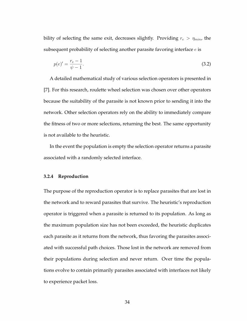
bility of selecting the same exit, decreases slightly. Providing re > ηmin, the
subsequent probability of selecting another parasite favoring interface e is
p(e)′ =re − 1
ψ − 1. (3.2)
A detailed mathematical study of various selection operators is presented in
[7]. For this research, roulette wheel selection was chosen over other operators
because the suitability of the parasite is not known prior to sending it into the
network. Other selection operators rely on the ability to immediately compare
the fitness of two or more selections, returning the best. The same opportunity
is not available to the heuristic.
In the event the population is empty the selection operator returns a parasite
associated with a randomly selected interface.
3.2.4 Reproduction
The purpose of the reproduction operator is to replace parasites that are lost in
the network and to reward parasites that survive. The heuristic’s reproduction
operator is triggered when a parasite is returned to its population. As long as
the maximum population size has not been exceeded, the heuristic duplicates
each parasite as it returns from the network, thus favoring the parasites associ-
ated with successful path choices. Those lost in the network are removed from
their populations during selection and never return. Over time the popula-
tions evolve to contain primarily parasites associated with interfaces not likely
to experience packet loss.
34
Such an approach is largely delay-agnostic, focused on avoiding loss. Since
avoiding loss is the primary objective, this may be reasonable. However, also
rewarding parasites experiencing favorable delay may be beneficial, as mini-
mizing delay is a secondary objective. This may be accomplished by extending
the parasite object to include a timestamp indicating when it was removed from
its population. When a parasite is returned to its population, the timestamp
may be used to determine the round-trip time (RTT). The RTT is the sum of the
forward-path delay and the reverse-path delay, which may not be symmetric.
The forward-path delay may be estimated if the destination router timestamps
the feedback packet. Because only the delay relative to other parasites for the
same destination is needed, the presence of clock skew between the destina-
tion router and the host router is not a significant limitation. This is discussed
in Chapter 8.2.
The operator selected for the delay-aware heuristic simply compares the
forward-path delay of a returning parasite to the forward-path delay of the
most recently returned parasite associated with the same destination. If the de-
lay is favorable for the returning parasite, its representation in the population is
increased by κ. This research does not explore finding the optimal value for κ,
only noting it should be less than the increment awarded for successful packet
delivery, as avoiding loss is the primary objective. In environments where de-
lay is particularly important, κ could be increased.
Listing 3.1 shows the delay-agnostic logic for returning a parasite and List-
ing 3.2 shows the delay-aware version.
35

Listing 3.1: Delay-agnostic return parasite operationreturn parasite (population p, parasite a){
e = egress link(a)r = get representation array(p)c = 1if (pcur(p) < high water(p))then
c = c + 1end ifr(e ) = r(e)+c
}
Listing 3.2: Delay-aware return parasite operationreturn parasite (population p, parasite a){
tc = forward path time(a)tp = get previous forward path time(p)e = egress link(a)r = get representation array(p)c = 1if (pcur(p) < high water(p))then
c = c + 1end ifif ( tc < tp)then
c = c + rewardend ofr(e ) = r(e)+cset previous forward path time(p,tc)
}
36
When the population reaches its high-water mark, ψhigh, one-for-one repro-
duction of returning parasites stops. Instead, the parasite is returned to the
population without reproducing. This is done to stabilize the population as it
reaches its maximum capacity. In the case of the delay-aware heuristic, the in-
crement for low delay continues to be awarded, even when the population is
full.
3.2.5 Mutation
In genetic algorithms, mutation[44] is used to explore parts of the landscape
otherwise not reachable through normal reproduction. Without mutation, the
population tends to converge to a homogeneous state where individuals vary
only slightly[69]. Mutated individuals often develop with fatal flaws and are
quickly eliminated from the population. However, occasionally a mutation re-
sults in an individual uniquely suited for the landscape. If this individual is
strong enough, future generations will tend to evolve to gain similar character-
istics.
For the genetic metaphor presented in this research there are limited options
for mutation. Parasite variation is restricted to the set of interfaces on the router.
However, mutation is still needed for the algorithm to explore new paths after
it has converged. Mutation occurs during the selection. The variable ν defines
the probability the parasite returned by the selection operator will be associated
with an interface randomly selected from the uniform distribution of all inter-
faces. Mutation only occurs if the parasite is going to be attached to a packet.
37

Because packets not carrying parasites are unable to provide feedback, there is
no point in using them to explore new solutions.
Larger values of ν allow the algorithm to more rapidly explore the topology
after a change occurs. However, increased packet loss is also associated with
larger values of ν, as packets will more frequently be routed along potentially
infeasible paths.
3.2.6 Sampling
As each parasite will require space in a packet’s header, attaching parasites
to every packet may create excessive overhead. In addition, the delivery of
feedback packets will create traffic that must compete with regular traffic for
network resources. In order to decrease this overhead, the heuristic only at-
taches parasites to a fraction of the packets traveling in the network. Packets
not receiving parasites are still routed by the parasite selection operator, but the
parasites used to only make the routing choice are neither removed from their
populations nor attached to the packet.
At least two approaches are available for selecting which packets will carry
parasites: traffic-based or time-based. The traffic-based approach would sam-
ple a fixed percentage of packets passing through the router while the time-
based approach would sample at a fixed rate, spacing samples evenly in time.
The tradeoffs associated with these two approaches are discussed below.
Sampling a fixed percentage of the packets passing through a router has a
few advantages. First, it is easy to implement and does not require additional
38

state be maintained in the population. Second, the number of samples is a func-
tion of the amount of traffic. Potentially, the routing will adapt more rapidly
if more samples are used. Therefore increased overhead might be justified for
larger flows of data.
One drawback to this approach is that the effective rate would be difficult
to control, as a packet sampled by one router must be “sampled” by all sub-
sequent routers in the path. Therefore the probability of sampling actually in-
creases at each hop in the forwarding path. This implies that the probability a
packet will carry parasites increases as a function of path length. For a sample
rate sr, the probability that the nth router attaches a parasite is 1 − (1 − sr)n.
Even when s is seemingly small, the probability of attaching a parasite may
be quite large if the path is relatively long. For example, if s = .05, after 10
hops the chance that the packet will carry parasites is approximately 40%. Be-
cause the goal for sampling was to decrease the overhead, this behavior may
be undesirable.
A second drawback for sampling based on load is the difficulty associated
with selecting a good value for ψmax. Because the rate at which parasites are
removed from the population is a function of the packet arrival rate and sr,
ψmax potentially needs to be a function of the packet arrival rate. If it is not,
it might be too small when traffic is heavy and too large when traffic is light.
The effect of the former is routing instability and the effect of the latter is slow
adaptation.
39

The second method of sampling is to temporally space samples at fixed in-
tervals. This has the advantage of not requiring ψmax to be a function of the
packet rate and overcomes the problem of the sample rate increasing for long
paths. It is slightly more difficult to implement; nevertheless, it is the method
selected for the heuristic.†
The sampling algorithm is implemented by storing the time the last par-
asite was taken from each population. Another sample is not taken from a
population until the sample interval has elapsed or until a packet arrives with
parasites attached. Whenever a parasite is taken from the population the last-
sample-time variable is updated. This method of sampling limits the effect of
long paths on the number of samples taken. The pseudo-code for packet for-
warding which includes fixed-interval sampling is shown in Listing 3.3.
While this approach is relatively simple, it may perform poorly when packet
arrivals are bursty. A more accurate fixed-rate sampling scheme could be at-
tempted that would account for burstiness, adjusting the sample interval as a
function of previous gap distribution. The benefits of such an approach are
unlikely to justify its complexity.
3.2.7 Summary of Operators and Parameters
This section presented many of the heuristic’s operators and parameters. One
of the difficulties associated with shortest-path routing is selecting link metrics.
†One desirable property of this sampling strategy is that it makes the behavior of the algorithm more predictable,as one does not need to consider the flow rate to determine convergence time, assuming the flow rate is large enoughto provide at least one packet during each sample interval.
40

Listing 3.3: Packet-forwarding function, including sampling logicforward packet(packet y){
address d = get destination(y)population p = get population(d)parasite l = choose parasite(p)interface e = get exit interface ( l )number s = sample rate
if parasites are attached(y) and red(e,y) {remove parasites(y)}
if queue is full (e,y) {remove parasite(p,l)l = choose parasite(p)e = get exit interface ( l )}
if parasites are attached(y) or sample gap(p) > now−last sample(p) {check for loops(y)remove parasite(p,l)push parasite(y,l )last sample(p)=now}
if queue is not full (e,y) {send packet(e,y)}
}
41

The heuristic approach eliminates the need for these metrics, but unfortunately
replaces them with an even larger set of parameters. This poses a significant
risk: perhaps these parameters will be more difficult to tune than the metrics
they replace. Indeed, due to the heuristic nature of the algorithm, it is diffi-
cult, if not impossible, to precisely describe in closed form the effect of these
parameters. However, the heuristic appears to be relatively insensitive to the
precise values chosen for these parameters. The parameter values initially cho-
sen, somewhat arbitrarily,‡ needed little modification throughout the simula-
tion studies presented in subsequent chapters. Table 3.1 lists the parameter
values used by this research, unless otherwise noted in the paper.
parameter value commentsψmax 2000 maximum size of the populationψhigh .95ψmax population size high-water markηmin 0 minimum number of parasites for each interfaceηinit 100 initial number of parasites for each interfaceω 1/ψmax sample interval in secondsν .005 probability of mutationκ .25 reward for low delay
Table 3.1: Parameter values used in this research
3.3 Congestion
Routing in the presence of congestion is one of the more challenging tasks for
any routing protocol. Often, difficult decisions must be made regarding which
packet to drop. The proposed heuristic has two mechanisms for dealing with
‡There was some logic in the order of magnitude selected for each variable. For example, most of the simulationshad 3 to 12 thousand packets being introduced each second. The size of the maximum population, ψmax was selectedsuch that it could easily be sampled in a period of one second without requiring every parasite to be sampled.
42

congestion. First, if an output queue is full, rather than dropping the packet,
alternate exits are sought for. Second, as the probability of reaching a congested
state increases, parasite strings are selectively dropped in an effort to influence
the routing decisions of upstream routers. This section provides an overview
of each mechanism.
3.3.1 Output Queue Overflow
Packet loss is typically caused by fixed-size output queues reaching their lim-
its. As additional packets are sent to the queue they must be dropped, be-
cause there is no room to store them. Assuming the queue space is not shared
between output interfaces, an assumption that should be valid on many dis-
tributed routing architectures, potentially another interface would be capable
of accepting the packet.
The heuristic reacts to this situation by destroying the parasite associated
with the interface having a full output queue and selecting a new parasite from
the population. The packet and second parasite are both destroyed if the in-
terface associated with the second parasite is full. This behavior increases the
speed at which the population can adapt to an overloaded link. If the router
did not stop with the second parasite and continued to query the population
until a feasible interface was found, the impact on the population associated
with the full interface might be too severe. Strong feedback such as this is often
associated with path oscillations.
43
3.3.2 Random Early Detect
Even when the output queue is not completely full, it may be helpful to include
a signaling mechanism to notify upstream routers of potential congestion. For
this reason the basic principles of Random Early Detection (RED)[33][32][8] are
incorporated into the heuristic.
When a RED-enabled router detects congestion, it attempts to signal the traf-
fic sources to decrease their send rates. This is referred to as backpressure[56].
A RED-enabled router detects congestion by monitoring the average output
queue length. Averaging allows short increases in the queue size to occur
without triggering backpressure. An exponentially-weighted moving average
(EWMA) low-pass filter is used by RED:
ave← (1− wq)ave+ wqq. (3.3)
The time constant of the low-pass filter is determined by the weight, wq. Deter-
mining the optimal value for wq is an open problem.
RED’s initial packet-marking probability, pb, is calculated as a linear function
of the average queue size
pb ← maxpave−minthmaxth −minth
, (3.4)
where maxp gives the maximum packet-marking probability, minth is the min-
imum threshold that must be exceeded before packets are to be marked, and
maxth is the maximum threshold, the point after which the marking probabil-
ity becomesmaxp. Simply using pb for the packet-marking probability has been
44

shown to result in a geometric spread of the intermarking time. Techniques to
make the intermarking time uniformly distributed have been proposed[33].
For Transmission Control Protocol (TCP)[73] traffic, the only backpressure
mechanism available for a standard router is to drop packets in an attempt to
influence TCP’s flow control. Nothing similar is available for User Datagram
Protocol (UDP) traffic. The proposed heuristic has a unique mechanism to in-
fluence the amount of traffic it is receiving from the source. As congestion is
detected, a router can delete the parasite string in a packet. As a result, parasites
belonging to the upstream routers will not be returned and their populations
will adapt as if the packet had been dropped. Thus, the approach is indepen-
dent of the transport protocol and would work for both TCP and UDP traffic.
The proposed heuristic also deviates from the standard RED algorithm in
that it does not use the queue length as an estimate of link utilization. Queue
length is a poor indicator of link utilization, especially in high-speed circuits.
The proposed heuristic relies on the router to keep track of average link utiliza-
tion over a small time period by measuring the output rate.
The algorithm presented in Listing 3.3 implements RED detection prior to
the full-output-queue check described in Section 3.3.1. The RED function was
placed there to ensure that feedback would be given to upstream routers when
a congested communications link was encountered, even if the second selection
found a less congested interface.
The RED parameters chosen for this research are maxp = .25, minth = .75,
and maxth = 1. Marking begins when the queue is 75% full. The maximum
45

number of parasites marked for the purpose of RED is 25%. These values were
chosen to ensure the heuristic could continue to operate when congested paths
had to be used. To accomplish this goal, the reproduction rate of the popula-
tion, a function of the returning packets, should be larger than the death rate
created by RED. Additionally, these values take into account the dampening ef-
fect of the population size. Typically, RED deals with dropping packets, which
greatly impacts the behavior of the senders; therefore, large values of wq are
used to allow bursting and small values of maxp are used to lower the num-
ber of drops. With the proposed heuristic, the impact is dampened, as only the
parasite string is being dropped, not the packet. Typically, truncating a parasite
string will influence the upstream routers’ populations only slightly.
3.4 Chapter Summary
This chapter has described the proposed heuristic. The concepts of parasites
and populations were introduced, as were the operators and parameters af-
fecting their existence. The formulation of the heuristic was accomplished by
modeling the genetic metaphor in a simple manner. While there appear to be a
large number of parameters, the heuristic should not require continued tuning
if reasonable values are selected initially. During the course of this research the
various parameters generally were not changed. Performance gains might be
achieved by selecting better values, but those chosen are sufficient to demon-
strate the feasibility of the heuristic. This chapter has provided the reader with
46

an understanding of the operation of the proposed heuristic. Subsequent chap-
ters will examine the performance of the proposed heuristic.
47

Chapter 4
Analysis of a Triplet Network
This chapter presents the reader with an analysis of the proposed heuristic on
a three-node triplet network. From a practical routing standpoint, the network
is relatively uninteresting. For any given source and destination pair, there is
only a single path, leaving little for the routing system to optimize. However,
due to this simplicity, the topology is useful for analyzing the heuristic.
In order to simplify the analysis, this chapter assumes the mutation rate is
set to zero; ηmin is used to ensure exploration of alternate paths. In addition, this
chapter only provides analysis for the delay-agnostic variation of the heuristic.
The network presented has a single loop-free path; therefore the delay-aware
variation offers no additional advantage.
This chapter begins with a description of the the triplet network and the
state model used to represent it. This is followed by observations and analysis
of the expected convergence time. The impact of various parameters on the
48

convergence time is discussed. Finally, a simple simulation system is presented
to confirm the model matches empirically obtained data.
4.1 Triplet Network State Model
2 31
a b
Figure 4.1: Triplet network topology
Consider the triplet shown in Figure 4.1. Assume all traffic originates on
node 2 and is destined for node 3. Node 2 maintains a population of parasites
associated with the destination of node 3. Because nodes 1 and 3 only have one
exit, the state of their populations will not affect the routing of packets. There-
fore, the entire state of the system is represented by the population on node 2.
This population will be referred to as “the population” for the remainder of this
chapter.
Initially the population will contain equal numbers of parasites favoring link
a and link b. Because node 1 has only one egress link, it will loop all packets it
receives from node 2 back toward node 2. Node 2 will be able to detect the loop
by searching the parasite string, and it will truncate the parasite string prior to
selecting a new parasite. Thus, parasites favoring link a will never be returned
to the population. Over time the the number of parasites in the population that
favor link a will decrease to ηmin.
49

Assuming the capacity of link b is not being exceeded, each parasite sent
on link b will return and be duplicated. Eventually, the number of parasites
associated with link b will reach ψmax − ηmin. At this point the probability of
taking link b will reach its upper limit of p(b) = 1 − ηminψmax
. Prior to reaching
this limit p(b) will reach an acceptable threshold, p(b) ≥ t, at which point the
population will have converged. Calculating the expected number of routing
choices prior to convergence is accomplished using a state model of the system.
4.2 State Analysis of the Triplet Network
The state of the entire system can be represented on a single two-dimensional
state-transition diagram. This is because node 2 is the only node with changing
state information. The instantaneous state of the system can be represented
by a discrete point on a grid, where the x-position represents the number of
parasites in the population that favor link b and the y-position represents the
number of parasites favoring link a. The state space for a system with only
two parasites is a triangle with vertices at (ηmin, ηmin), (ηmin, ψmax − ηmin), and
(ψmax − ηmin, ηmin). All points within the bounds of this triangle are potential
states for node 2. This state space is shown in Figure 4.2.
The state transitions for a node with two exits are shown in Figure 4.3. The
state will transition down when a parasite favoring the exit associated with the
y-axis is chosen. The probability of this happening, given a packet has arrived,
is yx+y
. The state will transition toward the left when a parasite favoring the exit
50

@@@@@@@@@@@@@@@@@@@
������
�����
(ψmax − ηmin, ηmin)
(ηmin, ψmax − ηmin)
(ηmin, ηmin)
(ηinit, ηinit)
Figure 4.2: State space for a router with two links
associated with the x-axis is chosen. The probability of this happening, given a
packet has arrived, is xx+y
. The state will transition two positions upward when
a parasite favoring the exit associated with the y-axis returns. The state will
transition two positions to the right when a parasite favoring the exit associated
with the x-axis returns.
For the triplet considered in this chapter, the probability of an upward state
transition is zero, as the link associated with the y-axis is not part of a loop-free
path to the destination. A parasite favoring link a will never be returned to
the population. This, combined with the non-zero probability of a downward
transition, implies that the number of parasites in the system favoring link a
will eventually decrease to ηmin. The potential state space is limited to ηinit ≤
51

����
����
�������� ���� ��������x, y x+ 2, y
x, y − 1
x, y + 2
x, y − 1
Figure 4.3: State transitions for a router with two links
y ≤ ηmin. The state transition diagram can be updated to remove the upward
transition, as its probability is zero.
Assuming the packet arrival rate is such that there are never two packets
in the network at the same time, the two horizontal state transitions can be
combined, as a state transition one unit to the left will always be immediately
followed by a state transition two units to the right. This combination results
in a unit transition to the right. The feasible state space may then be limited to
only include states right of the x-position of the initial population: x ≥ ηinit. The
updated possible state transitions for the triplet network are shown in Figure
4.4.
The state of the system follows a path beginning at (ηinit, ηinit) and end-
ing at (ψmax − ηmin, ηmin). The probability of using link b, p(b), is monotoni-
cally increasing, and can reach an acceptable value prior to reaching its limit at
p(b) = 1 − ηminψmax
. At this point the population is said to have converged. The
52

����
��������
p(a)
p(b)(x, y) (x+ 1, y)
(x, y − 1)
Figure 4.4: State transitions for node 2 in the triplet network
@@@@@@@@@@@@@@@@@@@
@@@@
��
(t ψmax, (1-t)ψmax)
Figure 4.5: The acceptable region of the state space
53

acceptable threshold value, t, where p(b) ≥ t, may be used to define the con-
vergence region, limited to all states below the line extending from the origin
to the point (tψmax, (1− t)ψmax). The angle of this line is atan(1−tt
). This region
is shown in Figure 4.5. Once the state has entered this region the system has
converged.
4.3 Time to Converge
To make the analysis independent of packet rate, the convergence time is de-
fined in terms of the number of probes required before the population con-
verges. A probe is defined to be a parasite’s life span on the network. Define
ex,y to be the expected number of probes required to converge from the start-
state of (x, y). ex,y is a function of the number of probes required by each of
its two adjacent states: state (x + 1, y) and state (x, y − 1). The probability, p,
of moving to state (x + 1, y) is equal to xx+y
, while the probability of moving to
state (x, y − 1) is yx+y
= 1 − p. The expected number of probes from ei,j is the
weighted sum of the number of probes expected for each of the adjacent states
plus one, to account for the probe required to move to a neighboring state.
ex,y = pex+1,y + (1− p)ex,y−1 + 1 (4.1)
Three boundary conditions exist for the above equation. First, when y = ηmin
and a parasite associated with the y-axis is selected, the state will transition
back to itself. The x transition remains the same. These state transitions are
shown in Figure 4.6. When y = ηmin the expected number of probes prior to
54
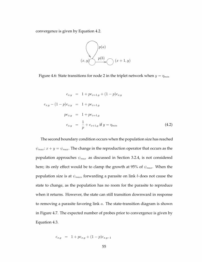
convergence is given by Equation 4.2.
���� ����p(b)
(x, y) (x+ 1, y)
p(a)
Figure 4.6: State transitions for node 2 in the triplet network when y = ηmin
ex,y = 1 + pex+1,y + (1− p)ex,y
ex,y − (1− p)ex,y = 1 + pex+1,y
pex,y = 1 + pex+1,y
ex,y =1
p+ ex+1,y if y = ηmin (4.2)
The second boundary condition occurs when the population size has reached
ψmax: x+ y = ψmax. The change in the reproduction operator that occurs as the
population approaches ψmax as discussed in Section 3.2.4, is not considered
here; its only effect would be to clamp the growth at 95% of ψmax. When the
population size is at ψmax, forwarding a parasite on link b does not cause the
state to change, as the population has no room for the parasite to reproduce
when it returns. However, the state can still transition downward in response
to removing a parasite favoring link a. The state-transition diagram is shown
in Figure 4.7. The expected number of probes prior to convergence is given by
Equation 4.3.
ex,y = 1 + pex,y + (1− p)ex,y−1
55

����
����p(a)
(x, y)
p(b)
(x, y − 1)
Figure 4.7: State transitions for node 2 in the triplet network when x+y = ψmax
(1− p)ex,y = 1 + (1− p)ex,y−1
ex,y =1
1− p+ ex,y−1 if x+ y = ψmax (4.3)
The final boundary condition occurs when the population is within the con-
vergence region, t < xx+y
. In this case, the expected number of probes prior to
convergence is zero.
ex,y = 0 if xx+y
> t (4.4)
By combining these boundary conditions the expected number of probes
may be calculated by progressing from right to left, bottom to top through the
feasible space, beginning with the point (ψmax− ηmin, ηmin). This point must be
in the target space, i.e., t < ψmax−ηminψmax
< 1− ηminψmax
, or the target t is unreachable.
If the target is reachable, eψmax−ηmin,ηmin is zero by Equation 4.4. The point to the
immediate left, (ψmax − ηmin − 1, ηmin), is either in the convergence region or,
if outside, may be obtained by using the value for eψmax−ηmin,ηmin and Equation
4.2. The other values on the line y = ηmin may be calculated in this manner,
moving from right to left (decreasing x). Once this row is complete, the value
for (ψmax − ηmin − 1, ηmin + 1) may be calculated using eψmax−ηmin−1,ηmin and
Equation 4.3. The remaining points to the left may be calculated using Equation
56

Listing 4.1: Routine to calculate the expected number of probes required toconverge for the triplet networkint EstimateProbes(target t ) {
i=rinitfor(y=rmin;y<=i;y++) {
for(x=pmax−x;x>=i;x−−) {p=x/(x+y)if p>=t e[x,y]=0else if ( y=rmin) then e[x,y]=1/p + e[x+1,y]else if ( x+y=pmax) then e[x,y]=1/(1−p) + e[x,y−1]else e[x,y]=1 + p∗e[x+1,y] + (1−p) ∗ e[x,y−1]end if
end forend forreturn e[ i , i ]}
4.1. This process repeats, moving up one row at a time, until the expected
number of probes for the initial state, eηinit,ηinit , is calculated. Pseudo-code for
this process is shown in Listing 4.1.
Using this routine the expected number of probes may be calculated given
values for t, ηmin, ηinit, and ψmax. For example, if ηmin = 25, ηinit = 100, and
ψmax = 1000 then the expected number of probes prior to 95% of the traffic
going over link b is 459.8. Maintaining the assumption that no two packets are
in the network at the same time and assuming a nominal round-trip time of
10ms, this could represent up to 5 seconds of delay prior to convergence.
4.3.1 Counting Routing Errors Only
The above analysis counts the total number of probes and does not distin-
guish between sending packets toward link a and sending packets toward link
57
b. Only those packets sent toward link a are routing “mistakes.” Therefore,
another relevant metric is the expected number of incorrectly routed packets
toward link a prior to the system converging. The expected number of probes
sent toward link amay be derived in a manner similar to how the total expected
number of probes was derived. The expected number of probes toward link a,
e′i,j , is the weighted sum of the number of probes expected for the state imme-
diately to the left, e′i+1,j , and one plus the expected number of probes from the
state immediately below, e′i,j−1. One is added to the quantity associated with
the state below to account for the probe sent toward link a which resulted in
the state transition. The former quantity is associated with a probe toward link
b and therefore does not include an increment. The boundary conditions may
be adjusted in a similar manner. The new set of equations can be formulated as
follows.
e′x,y =
0 if xx+y
> t
1p
+ e′x+1,y − 1 if y = ηmin
e′x,y−1 + 1 if x+ y = ψmax
pe′x+1,y + (1− p)(e′x,y−1 + 1) otherwise
(4.5)
Using the same values for ηmin, ηinit, and ψmaxas above, of the expected 459.8
probes, 80.0 are expected to be toward link a.
4.4 Empirical Results
The system can be simulated to validate these results. Because of the assump-
tion that only one packet is in the network at a time, the simulation system is
58
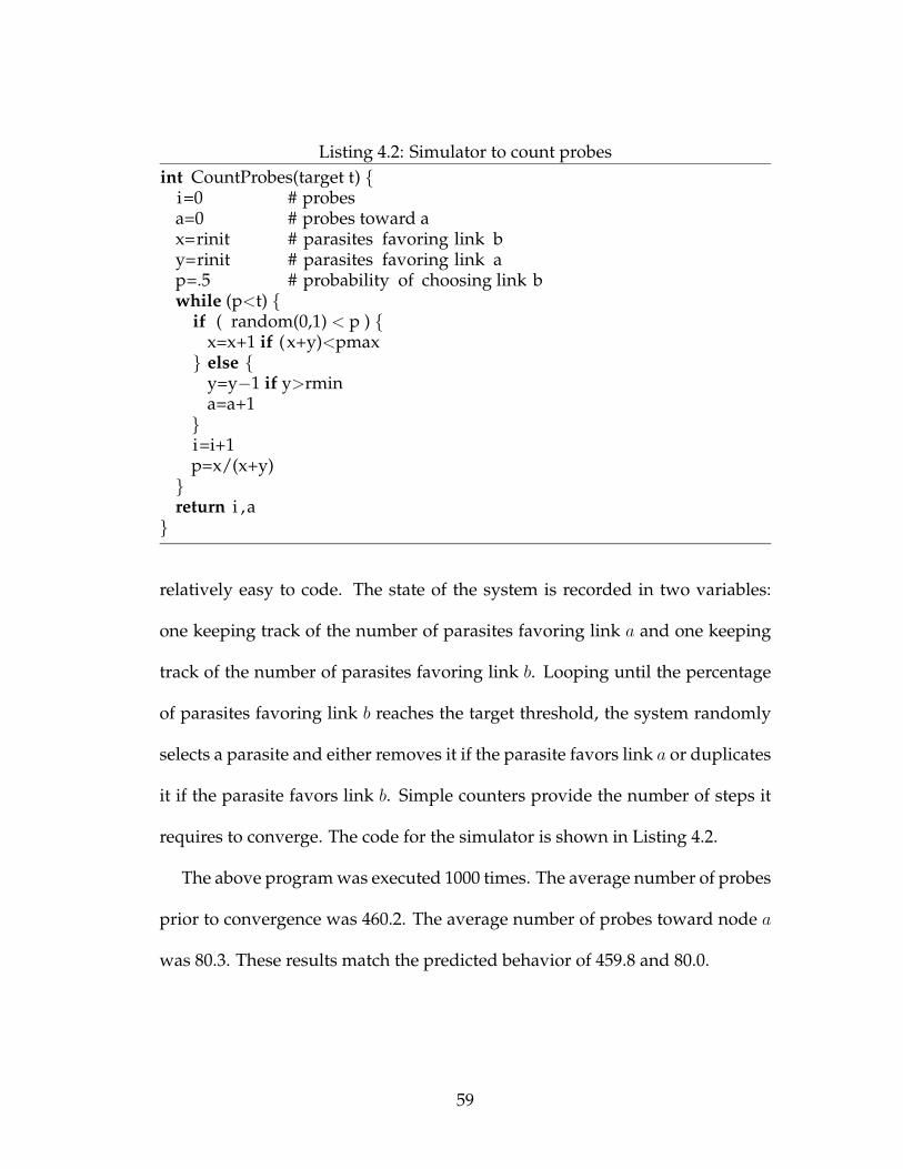
Listing 4.2: Simulator to count probesint CountProbes(target t) {
i=0 # probesa=0 # probes toward ax=rinit # parasites favoring link by=rinit # parasites favoring link ap=.5 # probability of choosing link bwhile (p<t) {
if ( random(0,1) < p ) {x=x+1 if (x+y)<pmax} else {
y=y−1 if y>rmina=a+1}i=i+1p=x/(x+y)}return i ,a}
relatively easy to code. The state of the system is recorded in two variables:
one keeping track of the number of parasites favoring link a and one keeping
track of the number of parasites favoring link b. Looping until the percentage
of parasites favoring link b reaches the target threshold, the system randomly
selects a parasite and either removes it if the parasite favors link a or duplicates
it if the parasite favors link b. Simple counters provide the number of steps it
requires to converge. The code for the simulator is shown in Listing 4.2.
The above program was executed 1000 times. The average number of probes
prior to convergence was 460.2. The average number of probes toward node a
was 80.3. These results match the predicted behavior of 459.8 and 80.0.
59

4.5 Understanding the Effects of the Parameters
One benefit of being able to express the performance of the heuristic in math-
ematical terms is the insight this provides into the effects of the heuristic’s pa-
rameters on its performance. This section focuses on the effects the values of
ηmin, ψmax, ηinit, and ω have on convergence.
4.5.1 Minimum Representation
The minimum representation of the population affects how often the algorithm
will explore a link that has previously performed poorly. Thus, one should ex-
pect that increases in ηmin should increase the number of steps prior to conver-
gence. If t is the convergence threshold, increasing ηmin beyond (1− t)ψmax will
result in a system that cannot converge, as the percentage of parasites favoring
link a will always be greater than t:
1− ηminψmax
< 1− (1− t)ψmaxψmax
< t.
Thus, the probability of sending traffic on the link toward b will always be less
than the convergence threshold, t. Lowering ηmin beyond a certain point also
has diminishing returns. The minimum value for ηmin may be estimated by
calculating the highest probability path from the initial state to when it enters
the convergence region. If ηinit is greater than (1 − t)ηmin, then it is impossible
for the system to reach ηmin parasites favoring link a prior to reaching its target
60

state. Therefore, lowering ηmin further will not have any effect on the expected
number of decisions prior to convergence. However, it will continue to affect
the steady-state rate at which bad decisions are made after convergence.
4.5.2 Maximum Population Size
The maximum population size may also affect the expected number of steps
to converge if it is small enough that the boundary condition for Equation 4.2
is met. When this happens the rate at which the system is approaching con-
vergence slows, as the successful parasites are not reproducing. As parasites
favoring link a are taken from the population, the state transitions downward
and once again parasites favoring link b may reproduce. In general, if it is
likely that the maximum population will be reached prior to convergence, con-
vergence takes slightly longer than if the population limit did not exist.
4.5.3 Initial Population
The value for ηinit needs to be somewhere between ηmin and ψmaxn
where n is the
number of interfaces: two in this case. If ηinit is too close to ηmin, it is likely that
the state of the system will hit the line y = ηmin. Being on this line represents
a slower convergence path because no additional parasites favoring link a can
be removed from the population. However, as ηinit approaches ψmax the like-
lihood of the population reaching ψmax increases. Reaching ψmax implies more
steps to convergence because good parasites are not being allowed to repro-
61

duce. Clearly an optimal value of ηinit exists for given values of ψmax and ηmin.
Finding this value is not considered in this research.
4.5.4 Sample Rate
The sample rate, ω, will affect the amount of time required to converge. All of
the previous discussion has counted the number of routing decisions. Implied
was that each of these probes involved attaching a parasite. With sampling,
not every packet will be assigned a parasite; therefore, the number of packets
routed prior to convergence will be higher than predicted in the above analy-
sis. Using fixed-interval sampling, if the system is sampling 480 packets per
second, one could expect the system to converge within 1 second. If it is sam-
pling 48 packets per second, the expected time to convergence would be 10
seconds. Convergence time is thus inversely proportional to the sampling rate.
4.6 Chapter Summary
This chapter has provided the reader with a state-based analysis of a simple
triplet network. The triplet network offers a topology for which meaningful
analytic results may be obtained. These results may be used to predict the con-
vergence time and also provide insight into the effects of some of the heuris-
tic’s parameters. In addition, the state model may be used to demonstrate loop
avoidance.
62
The topology, although simple enough to be easily analyzed, is not a good
representation of the types of networks in which the heuristic would realisti-
cally be used. The next two chapters discuss the performance of the heuristic
on increasingly complex topologies.
63
Chapter 5
Analysis of a Ring Network
This chapter examines the performance of the proposed heuristic on a specific
instance of a ring network. Like the triplet network, this topology is simple
enough that meaningful analytic results may be obtained. In addition to its
simplicity, the ring topology and the chosen link attributes combine to demon-
strate two shortcomings of typical shortest-path-based techniques: the inabil-
ity to non-uniformly distribute traffic across multiple paths and the inability
to adapt routing based on link utilization. The proposed heuristic is shown to
perform well with respect to both of these limitations.
The chapter begins with a derivation of the expected average delay of pack-
ets in the network: a function of both the amount of traffic and the way in
which it is distributed. Using these results the expected delay for each of the
three shortest-path scenarios may be predicted as a function of the size of the
input flows. These results are verified empirically using a discrete-time simula-
tion system. The heuristic is also simulated, and its performance is contrasted
64
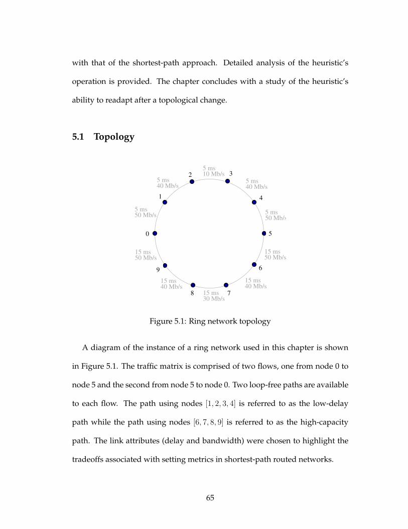
with that of the shortest-path approach. Detailed analysis of the heuristic’s
operation is provided. The chapter concludes with a study of the heuristic’s
ability to readapt after a topological change.
5.1 Topology
5 ms50 Mb/s
5 ms40 Mb/s
15 ms50 Mb/s
15 ms40 Mb/s
15 ms30 Mb/s
15 ms40 Mb/s
5 ms10 Mb/s
15 ms50 Mb/s
5 ms50 Mb/s
5 ms40 Mb/s
0
1
2 3
4
5
6
78
9
Figure 5.1: Ring network topology
A diagram of the instance of a ring network used in this chapter is shown
in Figure 5.1. The traffic matrix is comprised of two flows, one from node 0 to
node 5 and the second from node 5 to node 0. Two loop-free paths are available
to each flow. The path using nodes [1, 2, 3, 4] is referred to as the low-delay
path while the path using nodes [6, 7, 8, 9] is referred to as the high-capacity
path. The link attributes (delay and bandwidth) were chosen to highlight the
tradeoffs associated with setting metrics in shortest-path routed networks.
65
A path’s capacity is constrained by its minimum capacity link. In this case
the low-delay path is constrained to 10 Mb/s while the high-capacity path is
three times as large. The constraining link in each path is equidistant from
the path endpoints. This placement was chosen such that the path endpoints
could not detect congestion by observing local queue lengths. The magnitude
of the capacities was chosen to be large enough to represent realistic (although
small) wide-area network circuits while being small enough to have meaning-
ful queuing delay.
Two opposing flows are used to ensure that the impact of the overhead asso-
ciated with the feedback is felt. Congestion in the feedback path could poten-
tially affect both the adaptation and performance of the heuristic, as feedback
packets compete for resources with packets carrying data. Without opposing
flows, the feedback overhead would not have a negative effect.
In addition to having more capacity, the high-capacity path has larger prop-
agation delay. This highlights a potential dilemma for path selection: the opti-
mization of one objective may prevent the optimization of another. The prop-
agation delay on the high-capacity path was set to be three times that of the
low-delay path, making it significantly worse from the perspective of delay.
The magnitude of the propagation delays were chosen such that the composite
delay is on the order of what might be expected on a network path across the
United States.
66
5.1.1 Defining the Shortest Path
Defining the shortest path implies an understanding of what is considered
“short,” or what is to be optimized. Because of the values used for link ca-
pacities and delays, the path that minimizes delay is not the same path that
maximizes available capacity. The link metrics could be set as a function of de-
lay, in which case all traffic would be routed over the low-delay path; or they
could be set to be inversely proportional to the capacity, in which case all traffic
would flow over the high-capacity path. The only other option would be to
set the metrics such that each path had equal cost, dividing the traffic evenly
between the two paths. This would provide a compromise between delay and
capacity. In typical shortest-path algorithms there are no other options for dis-
tributing the flow. This presents a problem if the size of the flow exceeds the
capacity of the high-capacity path. To route this amount of traffic without loss,
the system needs to use both paths; but using them equally would result in loss
on the low-delay path once the flow exceeded 20 Mb/s. Non-uniform distri-
bution of the flows, referred to as non-minimal routing, would be capable of
facilitating nearly 40 Mb/s of traffic by placing one quarter of the traffic on the
low-delay path and routing the remaining three quarters of the traffic on the
high-capacity path.
In addition to the inability to split the traffic non-uniformly, typical shortest-
path approaches suffer from an inability to automatically adjust based on traf-
fic. Adaptive routing protocols, such as EIGRP[2], incorporate link utilization
67

into the link metrics, but, most widely used routing protocols are relatively
static and independent of load. For the ring network considered in this chap-
ter it would be beneficial to switch between the three possible shortest-path
solutions based on the size of the flow, even if the routing algorithm is non-
minimal. If the flow were less than 10 Mb/s, the low-delay path would be
used. If the flow were over 10 Mb/s and under 20 Mb/s, the traffic would be
split between both paths. For flows over 20 Mb/s, the traffic would be routed
over the high-capacity path. While it is easy to make this determination for
the simple topology being considered in this chapter, in larger, more complex
topologies, it is much more difficult to develop a strategy for changing paths
based on flow size. Automating this process while retaining stability is also a
difficult task.
5.1.2 Expected Delay Analysis
The delay along any path may be modeled as the sum of the processing, queu-
ing, transmission, and propagation delays. This research assumes that the pro-
cessing delay is negligible compared to the queuing and the propagation de-
lays. The transmission delay is embedded in the queuing delay formula as the
service time. For paths comprised of high-capacity wide-area network (WAN)
circuits with relatively low utilization, the delay is dominated by the propaga-
tion component. Only for lower capacity or heavily loaded circuits must the
contribution of queuing delay be considered.
68

For a system having a Poisson arrival process and exponentially distributed
packet sizes, the expected queuing delay can be approximated using Klein-
rock’s independence assumption[50] to be 1µC−λ where 1
µis the average packet
size, C is the link capacity in bits per second, and λ is the expected packet rate.
As µC approaches λ, the queuing delay increases until the queue’s capacity is
exceeded. At this point packet loss begins and the expected delay for packets
not being dropped levels off at qC
, where q is the queue size (in units compatible
to C). For this work, the queue size is set to be large enough to queue 333 ms
of traffic. Further increases in flow size will not affect the delay on the output
queue; only the packet loss will increase.
The expected delay on path p, where p is the vector of edges comprising the
path, may be expressed as
d(p) =|p|∑i=1
dpi + min[
1
µCpi − λpi,qpiCpi
](5.1)
where dpi is the propagation delay of the ith link on path p, Cpi is its capacity,
and qpi is its queue size. λpi is the packet rate presented to the ith link in the
path. In the case of the ring network, for all but the first link in the path, λpi is
the minimum of the flow rate presented to the previous link in the path and the
capacity (in packets) of that path. Let fp be the amount of traffic routed toward
the first link in path p.
λ1 = µfp (5.2)
λi = min[µCi−1, λi−1] (5.3)
69

The expected average delay for packets in a flow being routed over multi-
ple paths is the weighted average of the delay for each path. Let z(p) be the
probability of taking path p.
d =∑p∈P
z(p)d(p) (5.4)
P represents the set of all paths. Using these equations the expected delay
may be calculated for each possible combination of flow size and path distri-
bution. The expected delay may be plotted as a function of two variables: the
flow size and the probability of taking the low-delay path. Figure 5.2 plots the
expected delay against these two variables. In this plot the y-axis represents
the size of the flow and the x-axis represents the probability of a packet being
routed on the low-delay path. The z-axis represents the expected average delay.
The green surface represents the area in which the system does not experience
packet loss. The red surfaces represent combinations of load and flow distribu-
tion that result in packet loss. The height of each of these two red surfaces is a
function of queue size, which for this analysis was set to queue 333 ms of traf-
fic. Superimposed on the surface are four lines. The black line represents the
optimal delay for each value of offered load. The other three lines follow the
expected delays as a function of load for the three potential solutions available
if shortest-path routing is used: all the traffic going over the high-capacity path,
half the traffic going over each path, or all the traffic going over the low-delay
path.
70

high capacity pathequal split
low delay pathoptimal
00.25
0.50.75
1pdf 0
10
20
30
40
Mb/s
0
0.2
0.4
0.6
0.8
delay
Figure 5.2: Delay surface for routing in the ring network
This plot illustrates some of the limitations of standard shortest-path-based
approaches. Each of the three shortest-path solutions has a different region for
which it provides a suitable solution. For less than 10 Mb/s of flow, all the
packets may be routed on the low-delay path with no expected packet loss.
As the flow approaches 10 Mb/s, however, the delay increases and the better
solution becomes the one that divides the traffic evenly between both paths.
As the flow approaches 20 Mb/s, the half going over the low-delay path ap-
proaches 10 Mb/s and, once again, significant queuing delay occurs. This is
the point at which the best delay may be expected by routing all the traffic over
the high-capacity link. Typically, shortest-path algorithms do not adapt based
on link utilization; therefore, the safest choice would be to route all traffic on
the high-capacity path, as avoiding packet loss is typically more important than
minimizing delay.
71

Another limitation illustrated by this analysis is that none of the shortest-
path-based solutions is able to operate when more than 30 Mb/s of flow is
present. The inability to non-uniformly distribute traffic over multiple paths is
a key limitation of standard shortest-path-based techniques.
One may observe from this surface that there are drawbacks to precisely
selecting the optimal operating point. Assume that the routing system detects
20 Mb/s of flow. The optimal distribution for this amount of traffic puts 46% of
the traffic on the low-delay path. The average delay for the system is predicted
to be 54 ms. If the flow estimate was off by 10%, or if the flow changes by
10% to 22 Mb/s, the average delay will increase by almost 400% to 206 ms.
Similarly, if the algorithm used to calculate the optimal distribution was off
by 10%, resulting in a distribution of 50.6% of the traffic being routed on the
low-delay path, the average delay for the flow becomes 219 ms. Packets being
routed on the low-delay path experience an average delay of 359 ms.∗ This
sensitivity can be explained by observing the surface and the line representing
the optimal solution. The optimal solution follows a path relatively close to
areas for which the delay rapidly increases. Based on the confidence in the
flow predictions, one might choose to over-estimate the flow being input to the
optimization algorithm in order to avoid loss in the event the estimate was too
low. If there was little confidence in the ability to predict flow size accurately,
then the solution which distributes traffic in support of the maximum flow size
would be the safest choice.
∗This result assumes the queue size to be large enough to hold 333 ms of data.
72

5.2 Simulation Results for a Static System
The empirical study of the ring network begins with a study of the routing be-
havior for a static system, where neither the flows nor the topology changes.†
This section compares the predicted performance of the shortest-path tech-
niques to the actual performance measured with the simulator. This demon-
strates the analytic models are consistent with the empirical results and builds
some confidence in the accuracy of the simulator. The shortest-path trials are
followed by experiments using both the delay-agnostic and delay-aware heuris-
tics. Empirically observed properties of the heuristic are discussed.
5.2.1 Measured Delay for Shortest-Path Routing
The discrete-time network simulator was used to measure the average delays
experienced by packets in the ring network. Independent simulations were
performed with flows ranging in size from 1 Mb/s to 40 Mb/s. Each of the
three possible shortest-path flow distributions was simulated for 60 seconds.
Figures 5.3, 5.4, and 5.5 show predicted versus measured delays for routing the
flows over the low-delay path, over the high-capacity path, and equally across
both paths. Each line ends when packet loss exceeds 2%. The optimal average
delay is provided as a reference on each plot.
The correlation between the measured and the calculated delays suggests
that the system modeled by the simulator is consistent with the system mod-
†The flows and topology actually change once: they appear at time zero.
73

0
0.05
0.1
0.15
0.2
0 10 20 30 40
dela
y
�
Mb/s
optimalcalculatedsimulated
Figure 5.3: Measured vs. calculated delay for shortest-path approach using thelow-delay path
0
0.05
0.1
0.15
0.2
0 10 20 30 40
dela
y
�
Mb/s
optimalcalculatedsimulated
Figure 5.4: Measured vs. calculated delay for shortest-path approach using thehigh-capacity path
74
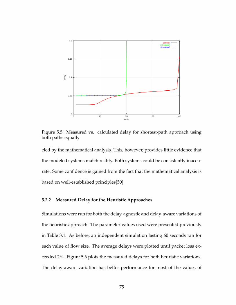
0
0.05
0.1
0.15
0.2
0 10 20 30 40
dela
y
�
Mb/s
optimalcalculatedsimulated
Figure 5.5: Measured vs. calculated delay for shortest-path approach usingboth paths equally
eled by the mathematical analysis. This, however, provides little evidence that
the modeled systems match reality. Both systems could be consistently inaccu-
rate. Some confidence is gained from the fact that the mathematical analysis is
based on well-established principles[50].
5.2.2 Measured Delay for the Heuristic Approaches
Simulations were run for both the delay-agnostic and delay-aware variations of
the heuristic approach. The parameter values used were presented previously
in Table 3.1. As before, an independent simulation lasting 60 seconds ran for
each value of flow size. The average delays were plotted until packet loss ex-
ceeded 2%. Figure 5.6 plots the measured delays for both heuristic variations.
The delay-aware variation has better performance for most of the values of
75
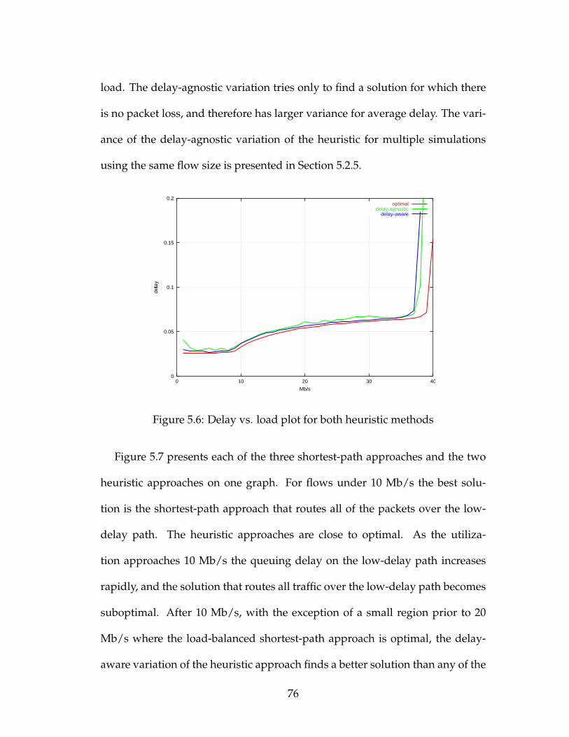
load. The delay-agnostic variation tries only to find a solution for which there
is no packet loss, and therefore has larger variance for average delay. The vari-
ance of the delay-agnostic variation of the heuristic for multiple simulations
using the same flow size is presented in Section 5.2.5.
0
0.05
0.1
0.15
0.2
0 10 20 30 40
dela
y
�
Mb/s
optimaldelay-agnostic
delay-aware
Figure 5.6: Delay vs. load plot for both heuristic methods
Figure 5.7 presents each of the three shortest-path approaches and the two
heuristic approaches on one graph. For flows under 10 Mb/s the best solu-
tion is the shortest-path approach that routes all of the packets over the low-
delay path. The heuristic approaches are close to optimal. As the utiliza-
tion approaches 10 Mb/s the queuing delay on the low-delay path increases
rapidly, and the solution that routes all traffic over the low-delay path becomes
suboptimal. After 10 Mb/s, with the exception of a small region prior to 20
Mb/s where the load-balanced shortest-path approach is optimal, the delay-
aware variation of the heuristic approach finds a better solution than any of the
76
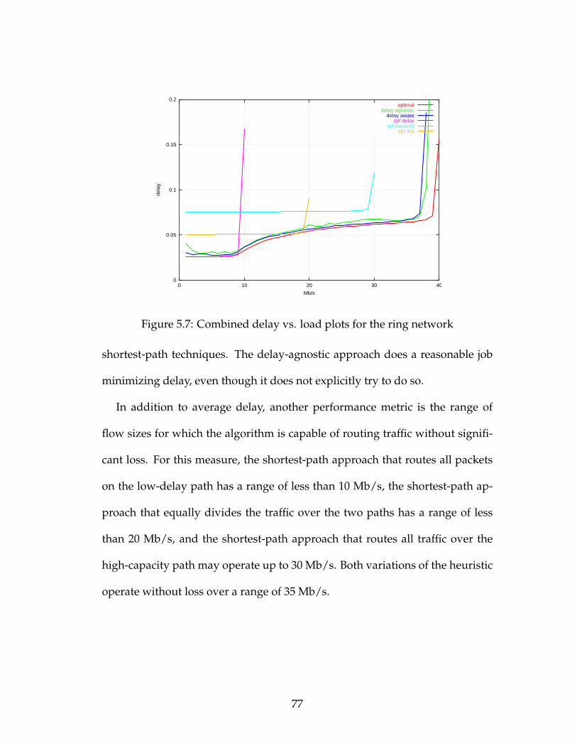
0
0.05
0.1
0.15
0.2
0 10 20 30 40
dela
y
�
Mb/s
optimaldelay-agnostic
delay awarespf delay
spf capacityspf mix
Figure 5.7: Combined delay vs. load plots for the ring network
shortest-path techniques. The delay-agnostic approach does a reasonable job
minimizing delay, even though it does not explicitly try to do so.
In addition to average delay, another performance metric is the range of
flow sizes for which the algorithm is capable of routing traffic without signifi-
cant loss. For this measure, the shortest-path approach that routes all packets
on the low-delay path has a range of less than 10 Mb/s, the shortest-path ap-
proach that equally divides the traffic over the two paths has a range of less
than 20 Mb/s, and the shortest-path approach that routes all traffic over the
high-capacity path may operate up to 30 Mb/s. Both variations of the heuristic
operate without loss over a range of 35 Mb/s.
77

5.2.3 Delay Variance Between Packets
Each of the above plots aggregate all the packet statistics for a given value of
flow size into a single point. Figures 5.8, 5.9, 5.10, 5.11, and 5.12 plot a sampling
(10%) of the delays experienced by packets in a 15 Mb/s flow going from node
0 to node 5. Packet loss is not shown on the plots. In the plot for the shortest-
path approach that routes traffic entirely over the low-delay path (Figure 5.8),
the effect of queuing is readily observed. The expected delay quickly rises to
the queuing capacity and then holds constant. Packets routed by the shortest-
path approach that sends all traffic over the high-capacity path (Figure 5.9)
have a very stable delay, that of the high-capacity path. In most instances this
is a desirable property, as packet ordering is likely to be affected if there is large
variation in the expected delay. Section 7.2.2 discusses the issue of reordering
in greater detail. Figure 5.10 shows the delays experienced by packets being
routed by the shortest-path approach that divides the traffic evenly over the
two paths. In this case the two distinct path delays can be observed.
The plots for both heuristic approaches have some interesting artifacts. Sim-
ilar to the shortest-path approach using both paths, large numbers of pack-
ets experience delay equal to one of the two path delays. A small number of
packets is grouped together with a delay equal to approximately the full-path
delay plus twice the link delays. These groupings are a result of packets being
looped back toward the source. Because each link along each path has the same
amount of delay, it does not matter which link loops the packet back: each will
78

0
0.1
0.2
0.3
0.4
0.5
0 10 20 30 40 50 60
dela
y
�
time
Figure 5.8: Sampled packet delay for a 15 Mb/s flow using the shortest-pathapproach routing all traffic on the low-delay path
0
0.1
0.2
0.3
0.4
0.5
0 10 20 30 40 50 60
dela
y
�
time
Figure 5.9: Sampled packet delay for a 15 Mb/s flow using the shortest-pathapproach routing traffic on the high-capacity path
79

0
0.1
0.2
0.3
0.4
0.5
0 10 20 30 40 50 60
dela
y
�
time
Figure 5.10: Sampled packet delay for a 15 Mb/s flow using the shortest-pathapproach routing traffic on both paths equally
0
0.1
0.2
0.3
0.4
0.5
0 10 20 30 40 50 60
dela
y
�
time
Figure 5.11: Packet delay for a 15 Mb/s flow using the delay-agnostic heuristic
80

0
0.1
0.2
0.3
0.4
0.5
0 10 20 30 40 50 60
dela
y
�
time
Figure 5.12: Packet delay for a 15 Mb/s flow using the delay-aware heuristic
add a constant amount of delay to the packet. If each link had different delays
the groupings would be harder to observe. If the second node in the path is
the one to loop the packet back, then node 0 again may choose between the
two paths. This results in groupings of packet delays 10 ms above the delay
grouping for the low-delay path and 30 ms above the delay grouping for the
high-capacity path. It may be observed in the plots for the heuristic that neither
path is utilized enough to have significant queuing delay.
The distribution of packet delays is difficult to observe in the previous plots
because multiple points may land directly on top of each. A better indicator of
delay distribution may be obtained from a boxplot showing Tukey’s 5-number
summary[80] for each method.‡ Boxplots for flow sizes of 5, 15, 25, and 35 Mb/s
are shown in Figures 5.13, 5.14, 5.15, and 5.16 respectively. In these and all
‡Tukey’s 5-number summary is the minimum, lower quartile, median, upper quartile, and maximum.
81

subsequent figures, the label ga is the delay-agnostic variation of the heuristic,
gd is the delay-aware version, sd is the shortest-path algorithm with metrics set
to route all its traffic on the low-delay path, sm is the shortest-path algorithm
with metrics set to distribute the traffic equally on the two paths, and sc is
the shortest-path algorithm with metrics set to route all the traffic on the high-
capacity path.
ga gd sd sm sc
0.0
0.1
0.2
0.3
0.4
0.5
dela
y
Figure 5.13: Tukey boxplots for all approaches with 5 Mb/s flows
These boxplots illustrate that the spread of packet delay for the heuristic
approaches is wider than for the shortest-path approaches. The variance in
the shortest-path approaches is primarily a function of the packet sizes, which
are exponentially distributed. Some variance might also be attributed to occa-
sional queuing. For the shortest-path approach that uses both paths equally, the
packet-delay distribution is bimodal with a peak at each of the path’s propaga-
tion delays. The spread in the heuristic methods is caused by multiple factors.
82

ga gd sd sm sc
0.0
0.1
0.2
0.3
0.4
0.5
dela
y
Figure 5.14: Tukey boxplots for all approaches with 15 Mb/s flows
ga gd sd sm sc
0.0
0.1
0.2
0.3
0.4
0.5
dela
y
Figure 5.15: Tukey boxplots for all approaches with 25 Mb/s flows
83

ga gd sd sm sc
0.0
0.1
0.2
0.3
0.4
0.5
dela
y
Figure 5.16: Tukey boxplots for all approaches with 35 Mb/s flows
In addition to the variance mentioned above, packets routed by the heuristic
might experience large delay variance as a result of suboptimal path selection.
The heuristic uses mutation to explore other potential solutions, and such mu-
tation causes some percentage of the packets to be routed along suboptimal
paths. For these experiments the mutation rate was set to be .5%. This implies
the probability of a packet traveling five hops without taking a “mutant” path
is .9955 = .975. However, since mutation randomly selects an egress link, and
one of the two choices is good, the probability of making a bad choice after con-
vergence is 1 − .99755 = .9876. In a network with longer paths or nodes with
higher degrees, the probability of “bad mutation” increases.
84

5.2.4 Population Stability over Time
The populations in the heuristic approach change over time. The stability of
these populations is important if consistent routing performance is desired.
This section evaluates the stability of the populations. The shortest-path tech-
niques are stable over time due to the fact that the routing does not change.
Figures 5.17, 5.18, 5.19, and 5.20 plot the probability that node 0 will route to-
ward node 1 traffic destined to egress on node 5 (node 0 PDF). The node 1 PDF
is plotted versus time for flow sizes of 5 Mb/s, 15 Mb/s, 25 Mb/s, and 35 Mb/s
respectively. In each plot, the optimal percentage of traffic to send toward node
1 is shown, as are the upper and lower values for the PDF for which no packet
loss is expected. This feasibility region narrows as the flow size increases. The
shortest-path PDFs are not included, but could be represented by three straight
lines at y = 0 (all traffic over the high-capacity path), y = .5 (equally dividing
the traffic over both paths), and y = 1 (all traffic over the low-delay path).
The PDFs for each of the operating points are stable for both variations of the
heuristic. The approach attempting to minimize delay experiences some minor
oscillations as it continues to probe the low-delay path for additional capac-
ity. The delay-agnostic variation of the heuristic exhibits good stability. This is
because there is no mechanism beyond mutation encouraging the population
to change once it has found a loss-free solution. The exception to this is at 39
Mb/s, where the approach seems to bounce around in search of the feasible
solution. This result is shown in Figure 5.21.
85
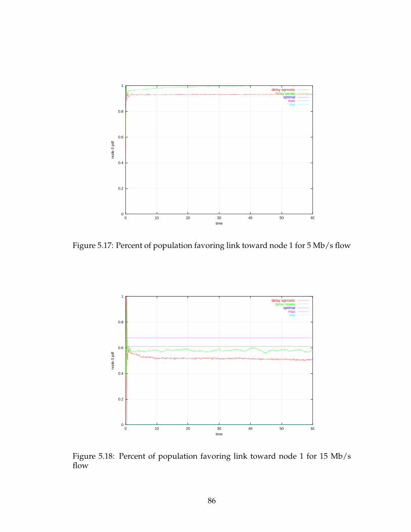
0
0.2
0.4
0.6
0.8
1
0 10 20 30 40 50 60
node
0 p
df
time
delay agnosticdelay aware
optimalmaxmin
Figure 5.17: Percent of population favoring link toward node 1 for 5 Mb/s flow
0
0.2
0.4
0.6
0.8
1
0 10 20 30 40 50 60
node
0 p
df
time
delay agnosticdelay aware
optimalmaxmin
Figure 5.18: Percent of population favoring link toward node 1 for 15 Mb/sflow
86

0
0.2
0.4
0.6
0.8
1
0 10 20 30 40 50 60
node
0 p
df
time
delay agnosticdelay aware
optimalmaxmin
Figure 5.19: Percent of population favoring link toward node 1 for 25 Mb/sflow
0
0.2
0.4
0.6
0.8
1
0 10 20 30 40 50 60
node
0 p
df
time
delay agnosticdelay aware
optimalmaxmin
Figure 5.20: Percent of population favoring link toward node 1 for 35 Mb/sflow
87

0
0.2
0.4
0.6
0.8
1
0 10 20 30 40 50 60
node
0 p
df
time
delay agnosticdelay aware
optimalmaxmin
Figure 5.21: Percent of population favoring link toward node 1 for 39 Mb/sflow
In general it may be concluded that the heuristic approaches are reasonably
stable for this ring topology. However, questions remain regarding the stability
of the approaches in the presence of a changing topology or traffic matrix. In
these cases it may be desirable for the population on node 0 to adapt quickly in
response to the external changes. However, rapid response may lead to hyper-
sensitivity and oscillations. A study of the behavior of the heuristic in a more
fluid environment is included in Section 5.3.
5.2.5 Solution Variance for the Delay-Agnostic Heuristic
Because the delay-agnostic heuristic seeks only to minimize loss and does not
consider the delay experienced by the packets, one would expect the solution
chosen by this approach to be randomly selected from the PDFs for which loss
88

is not expected. This section attempts to quantify the randomness of the solu-
tions chosen by this heuristic.
To study the delay variance of the delay-agnostic variation of the heuristic,
100 simulations were run for flow sizes of 5, 15, 25, and 35 Mb/s. Histograms
for each are shown in Figures 5.22, 5.23, 5.24, and 5.25.
ave delay (ms)
Fre
quen
cy
28 30 32 34 36 38 40
05
1015
20
Figure 5.22: Histogram for 100 runs of delay-agnostic heuristic with 5 Mb/sflows
These results demonstrate that the delay-agnostic approach operates within
the feasibility envelope, as one would expect. Although it does not seek to min-
imize delay, the approach tends toward the low-delay solutions. This is most
likely due to the fact the approach shares some characteristics with simulated-
annealing-based techniques[60]. As the populations move from their initial
uniform distribution toward a distribution which does not result in packet loss,
they do so in relatively small increments.
89
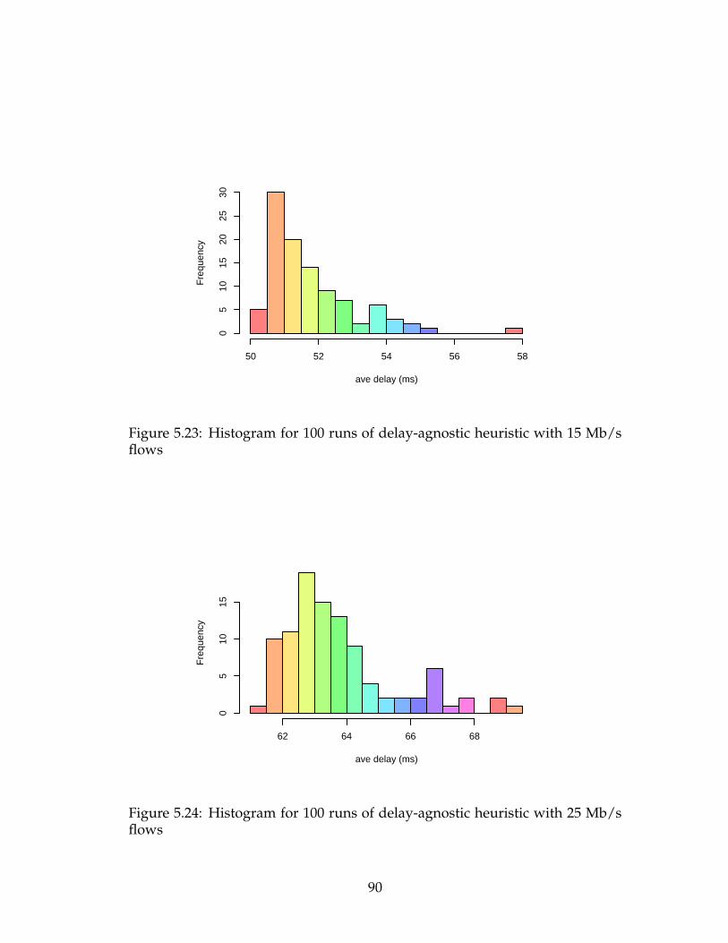
ave delay (ms)
Fre
quen
cy
50 52 54 56 58
05
1015
2025
30
Figure 5.23: Histogram for 100 runs of delay-agnostic heuristic with 15 Mb/sflows
ave delay (ms)
Fre
quen
cy
62 64 66 68
05
1015
Figure 5.24: Histogram for 100 runs of delay-agnostic heuristic with 25 Mb/sflows
90

ave delay (ms)
Fre
quen
cy
66 68 70 72
010
2030
40
Figure 5.25: Histogram for 100 runs of delay-agnostic heuristic with 35 Mb/sflows
5.2.6 Static Ring Topology Summary
This section has demonstrated that the proposed heuristic is capable of finding
near-optimal solutions for routing in the ring network in a static environment.
This is an important conclusion; without it there would be little purpose in
studying the more difficult problem of routing in a dynamically changing net-
work topology. Real-world networks are rarely static; rather, they are fluid and
changing. The next section of this chapter examines the behavior of the heuris-
tic in the presence of change.
5.3 Simulation Results for a Dynamically Changing Network
The above analysis focuses entirely on a static system, as neither the flows nor
the topology is changing during the simulation. This section examines the be-
91
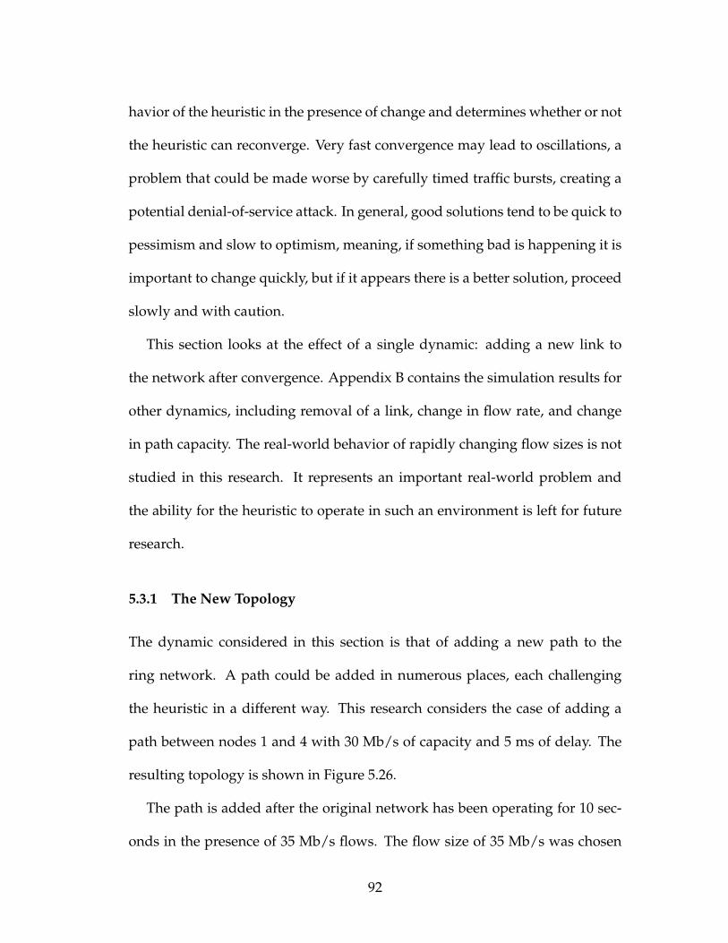
havior of the heuristic in the presence of change and determines whether or not
the heuristic can reconverge. Very fast convergence may lead to oscillations, a
problem that could be made worse by carefully timed traffic bursts, creating a
potential denial-of-service attack. In general, good solutions tend to be quick to
pessimism and slow to optimism, meaning, if something bad is happening it is
important to change quickly, but if it appears there is a better solution, proceed
slowly and with caution.
This section looks at the effect of a single dynamic: adding a new link to
the network after convergence. Appendix B contains the simulation results for
other dynamics, including removal of a link, change in flow rate, and change
in path capacity. The real-world behavior of rapidly changing flow sizes is not
studied in this research. It represents an important real-world problem and
the ability for the heuristic to operate in such an environment is left for future
research.
5.3.1 The New Topology
The dynamic considered in this section is that of adding a new path to the
ring network. A path could be added in numerous places, each challenging
the heuristic in a different way. This research considers the case of adding a
path between nodes 1 and 4 with 30 Mb/s of capacity and 5 ms of delay. The
resulting topology is shown in Figure 5.26.
The path is added after the original network has been operating for 10 sec-
onds in the presence of 35 Mb/s flows. The flow size of 35 Mb/s was chosen
92

5 ms50 Mb/s
5 ms40 Mb/s
15 ms50 Mb/s
15 ms40 Mb/s
15 ms30 Mb/s
15 ms40 Mb/s
5 ms10 Mb/s
15 ms50 Mb/s
5 ms50 Mb/s
5 ms40 Mb/s
0
1
2 3
4
5
6
78
9
5 ms30 Mb/s
Figure 5.26: Ring topology with added link
to cause the network to be running near peak capacity. Once the new path is
added, node 0 may send more traffic toward node 1. Since the two paths that
pass through node 1 have 40 Mb/s of combined capacity with lower delay to
that experienced on the path through node 9, nearly all the traffic in the flow
from node 0 to node 5 should be routed toward node 1. Figure 5.27 shows the
measured behavior of both variations of the heuristic.
For the first few seconds the delay-agnostic variation of the heuristic looks
for a loss-free solution. After about 5 seconds, node 0 converges on a solution
that sends approximately 8.75 Mb/s of traffic toward node 1 and 26.25 Mb/s
toward node 9. This distribution of traffic results in no steady-state packet
loss, and the solution is stable through the first 10 seconds. Once the new
link is added the heuristic does not seek to reconverge: it is not experiencing
93
0
0.2
0.4
0.6
0.8
1
0 10 20 30 40 50 60
% p
opul
atio
n fa
vorin
g lin
k to
nod
e 1
time
delay-agnosticdelay-aware
Figure 5.27: Portion of population on node 0 favoring link toward node 1,delay-aware and delay-agnostic
packet loss and because it is delay-agnostic there is nothing else to influence it
to change.
The delay-aware variation of the heuristic operates in a similar way for the
first 10 seconds, finding a near-optimal solution. However, after the new link
is added the delay-aware heuristic slowly begins to adapt to use the newly cre-
ated path. The behavior is in accordance with the design goal to react quickly
to negative news and react slowly to positive news. Because the system has
found a loss-free path, moving with caution to a new path with less delay is
acceptable.
An important question to answer is whether the behavior of the delay-aware
variation of the heuristic can be accurately predicted. Is there a model that
describes how fast it will learn to use the new path? The following section
94
presents such a model. This analysis will focus on parasites associated with the
destination of node 5.
5.3.2 Understanding the Effect of Round-Trip Time
First observe that the behavior of nodes 0 and 1 are interdependent. Node 0
relies on node 1 adapting such that traffic sent to it by node 0 is not dropped.
Node 1 relies on node 0 sending it enough traffic to meet its minimum sampling
interval. In addition, node 1’s convergence will be hastened if node 0 sends
too much traffic, triggering the RED operator on the downstream paths. This
section focuses on the effect of round-trip time (RTT) on the populations. The
following section will incorporate the effect of the RED operator into the final
predictive model.
The delay-aware variation of the heuristic is able to react to the topology
change because its reproduction operator rewards parasites that experience
low delay. Because the new path has the lowest delay, the relative represen-
tation of parasites favoring this path is expected to increase. The rate of this
increase can be accurately predicted.
Consider the population on node 1. Define the variable n1,2 to be the number
of parasites on node 1 favoring the link toward node 2. n1,4 is defined to be the
number of parasites on node 1 favoring the link toward node 4. Assume further
that node 1’s population has reached its maximum, ψ = ψmax, and therefore
the reproduction loop is only rewarding parasites that return faster than the
previous parasite.
95
From the perspective of node 1, if a returning parasite had been sent toward
node 2 (the longer-delay path) it has about a 50% chance of having experienced
less delay than the previous parasite, providing the previous parasite was also
sent on that same path. Otherwise, if the previous parasite was sent directly to-
ward node 4, there is little chance the returning parasite experienced less delay.
Define p1,2 to be the probability that a parasite sent toward node 2 experiences
less delay than the previous parasite.
p1,2 = .5n1,2
ψ(5.5)
Similarly, if the returning parasite had been sent directly to node 4 using
the new link and the previous parasite was sent toward node 2, the returning
parasite will nearly always have lower delay. If the previous parasite was sent
toward node 4, then the returning parasite has a 50% chance of having lower
delay.
p1,4 = .5n1,4
ψ+n1,2
ψ=.5n1,4 + n1,2
ψ(5.6)
The reward for having lower delay than the previous parasite is κ. The ex-
pected increment to node 1’s population favoring the link toward node 2, i1,2,
is κtimes the probability that the packet was sent to node 2 multiplied by p1,2.
i1,2 = κn1,2
ψp1,2 = κ
n1,2
ψ(.5n1,2
ψ) (5.7)
The expected increment to node 1’s population associated with the new link,
i1,4, can be expressed in a similar way.
i1,4 = κn1,4
ψp1,4 = κ
n1,4
ψ
.5n1,4 + n1,2
ψ(5.8)
96

In general, the expected increment associated with a parasite type is equal to
the product of the probability that parasite type is chosen, the probability that
the parasite will have favorable delay to the previous parasite, and κ. Using
this logic the expressions for node 0 can be derived.
5.3.3 Predicting the Effect of the RED operator
The RED operator is present to influence upstream routers to send less traffic
on a congested path. In this topology the link between nodes 2 and 3 is likely to
experience some congestion as node 0 increases the amount of traffic it sends
towards node 1. In addition, once node 0 is able to send most of its traffic
toward node 1, the RED operator will also drop some parasites being sent on
the new link toward node 4.
To predict the impact of the RED operator the amount of load on each of
the links must be estimated. The amount of traffic being sent to node 1 from
node 0, τ0,1, is the flow rate, |f |, multiplied by the percentage of parasites in the
population that favor the link toward node 1.
τ0,1 = |f |n0,1
ψ(5.9)
Similarly, the amount of traffic being sent by node 1 on the link toward node 2
can be defined in terms of τ0,1.
τ1,2 = τ0,1n1,2
ψ= |f |
(n1,2
ψ
)(n0,1
ψ
)(5.10)
97

Since node 2 will send nearly all its traffic to node 3, τ2,3 will roughly be equal
to τ1,2. The amount of traffic being sent by node 1 on the link toward node 4 is
τ1,4 = τ0,1n1,4
ψ= |f |
(n1,4
ψ
)(n0,1
ψ
). (5.11)
The utilization on the link between nodes 2 and 3 is τ2,3c2,3
where c2,3 is the
capacity of the link between nodes 2 and 3. The probability of node 2’s RED
operator truncating the parasite string, using the RED parameters defined in
Section 3.3.2, is
ρ2,3 =
τ2,3c2,3− .75 if τ1,2
c2,3> .75
0 otherwise.(5.12)
Because the link between nodes 2 and 3 is constrained to 10 Mb/s, it is unlikely
that there will be enough traffic on the link from node 1 to node 2 for node 1’s
RED operator to truncate a parasite string on a packet being sent to node 2.§
However, the probability of node 1’s RED operator truncating a parasite string
for a packet being sent on the new link is non-zero, and may occur close to
the end of convergence when node 0 is trying to send nearly 35 Mb/s over the
combined 40 Mb/s of path capacity.
ρ1,4 =
τ1,4c1,4− .75 if τ1,4
c1,4> .75
0 otherwise(5.13)
From node 0’s perspective, the probability that a parasite sent toward node 1
gets dropped is one minus the probability that the parasite is not dropped by a
RED operator. The probability that a parasite is not dropped by a RED operator
is the joint probability that node 1 does not drop the parasite string for packets
§This might not be the case if other flows were present.
98
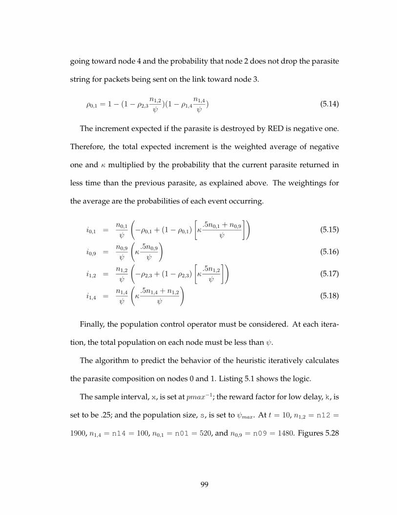
going toward node 4 and the probability that node 2 does not drop the parasite
string for packets being sent on the link toward node 3.
ρ0,1 = 1− (1− ρ2,3n1,2
ψ)(1− ρ1,4
n1,4
ψ) (5.14)
The increment expected if the parasite is destroyed by RED is negative one.
Therefore, the total expected increment is the weighted average of negative
one and κ multiplied by the probability that the current parasite returned in
less time than the previous parasite, as explained above. The weightings for
the average are the probabilities of each event occurring.
i0,1 =n0,1
ψ
(−ρ0,1 + (1− ρ0,1)
[κ.5n0,1 + n0,9
ψ
])(5.15)
i0,9 =n0,9
ψ
(κ.5n0,9
ψ
)(5.16)
i1,2 =n1,2
ψ
(−ρ2,3 + (1− ρ2,3)
[κ.5n1,2
ψ
])(5.17)
i1,4 =n1,4
ψ
(κ.5n1,4 + n1,2
ψ
)(5.18)
Finally, the population control operator must be considered. At each itera-
tion, the total population on each node must be less than ψ.
The algorithm to predict the behavior of the heuristic iteratively calculates
the parasite composition on nodes 0 and 1. Listing 5.1 shows the logic.
The sample interval, x , is set at pmax−1; the reward factor for low delay, k , is
set to be .25; and the population size, s , is set to ψmax. At t = 10, n1,2 = n12 =
1900, n1,4 = n14 = 100, n0,1 = n01 = 520, and n0,9 = n09 = 1480. Figures 5.28
99

Listing 5.1: Routine to predict the convergence of node 0 after new link is addedfor t=10 to 60 step x {
u23=(z∗(n01/s)∗(n12/s))/c23if (u12>.75) {
r12=u12−.75} else {
r12=0}
u14=(z∗(n01/s)∗(n14/s))/c14if (u14>.75) {
r14=u14−.75} else {
r14=0}
r01=1−(1−r12∗(n12/s))∗(1−r14∗(n14/s));
i01=(n01/s)∗(−r01+(1−r01)∗(k∗(.5∗n01+n09)/s));i09=(n09/s)∗(−0 +(1−0) ∗(k∗(.5∗n09 )/s ));i14=(n14/s)∗(−0 +(1−0) ∗(k∗(.5∗n14+n12)/s));i12=(n12/s)∗(−r12+(1−r12)∗(k∗(.5∗n12 )/s ));
n01=n01+i01n09=n09+i09n12=n12+i12;n14=n14+i14;
if (n12+n14>s) {n12=n12−n12/sn14=n14−n14/s}if (n01+n09>s) {
n01=n01−n01/sn09=n09−n09/s}}
100

and 5.29 plot the predicted values against the measured values for nodes 1 and
0.¶ In each case the behavior of the heuristic was accurately predicted.
0
0.2
0.4
0.6
0.8
1
0 10 20 30 40 50 60
% p
opul
atio
n fa
vorin
g lin
k to
nod
e 4
time
predictedmeasured
Figure 5.28: Portion of population on node 1 favoring link toward node 4, pre-dicted and measured
5.3.4 Dynamic Ring Topology Summary
This section has demonstrated the heuristic’s ability to adapt when a new link
is added to the topology. The delay-agnostic variation did not adapt, as it had
already found a solution with no packet loss and had no reason to search for
a new solution. The delay-aware variation of the heuristic, however, was able
to converge to make use of the new link. This section demonstrated that the
rate at which the new path is adopted can be accurately predicted. The rate
of convergence for the delay-aware variation of the heuristic, 30-40 seconds,
¶The sampling algorithm was modified slightly from what was presented earlier to cause the samples to be takenat more regular intervals. The original method tended to sample less frequently. Regressive analysis will be providedin a future paper.
101
0
0.2
0.4
0.6
0.8
1
0 10 20 30 40 50 60
% p
opul
atio
n fa
vorin
g lin
k to
nod
e 1
time
predictedmeasured
Figure 5.29: Portion of population on node 0 favoring link toward node 1, pre-dicted and measured
might seem large. However, this is consistent with the design goal of being
slow to optimism. As long as packets are not being dropped, slow adaptation
is acceptable.
5.4 Chapter Summary
This chapter examined the performance of the proposed heuristic on a specific
instance of a ring network. This topology was simple enough to allow deriva-
tion of meaningful analytic results. In addition, with careful selection of the
ring’s parameters, the topology was useful in demonstrating some of the lim-
itations present in static shortest-path-based routing techniques, namely, the
inability to non-uniformly distribute traffic and the inability to adapt based on
load. The proposed heuristic method was shown to be capable of discovering
102
reasonable routing solutions, attributes of which included non-uniform load
sharing and real-time adaptation based on network load. While both the delay-
aware and delay-agnostic variations performed reasonably well through most
of the trials, the delay-aware variation consistently outperformed the delay-
agnostic version. The delay-aware variation exhibited many desirable prop-
erties, including routing that resulted in better average delay and the ability
to converge to a new solution when the current solution was not experiencing
packet loss. Advantages of the delay-agnostic heuristic include implementa-
tion simplicity and reduced packet overhead. While the ring topology studied
was useful for its analytic properties, it is not representative of a generalized
network. The following chapter will examine a more realistic topology.
103

Chapter 6
Analysis of a Regional Network
The previous topologies have been useful in establishing the baseline perfor-
mance of the heuristic. However, because of their simplicity, they are poor
representations of real-world networks. In each case the network topology and
traffic matrix were carefully constructed to explore specific properties of the
heuristic. This chapter evaluates the performance of the heuristic on a more
realistic network, a topology similar to what might be found in a nationwide
network in the United States. In addition to the topology being more realistic,
the distribution of link sizes and delays were chosen to be less uniform than
those used in the previous chapters. While this is a step toward a more realistic
topology, it still lacks the intricacies and complexities of a real-world network,
mainly due to the simplified traffic flows. As before, the traffic models used
for this analysis assume exponentially distributed packet sizes and a Poisson
arrival process.
104

The chapter is organized as follows: First, the topology of the network is de-
scribed. Next, the heuristic is analyzed with a single flow, multiple flows, and
finally, flows between every pair of routers in the network. For each of these ex-
periments, both the shortest-path solution and the optimal solution were found
and contrasted with the results of the heuristic. For the shortest-path calcula-
tion, the link metrics were set to be the propagation delay of the links. The
metrics of the links were not adjusted further to account for traffic conditions.
This was done to keep the analysis as objective as possible. Real-world net-
works typically have metrics set by human operators who employ various ad-
hoc procedures to determine acceptable metric values. Such behavior is hard
to model or quantify. The chapter concludes with a summary of the results.
6.1 Topology
The network topology considered in this chapter roughly approximates the
topology of a regional network with points of presence in large metropolitan
areas. Although a typical real-world regional network would have multiple
routers in each switch site, the topology designed for this analysis only uses
one router per switch site. This was done to keep the problem simple. The
topology of the network is shown in Figure 6.1.
The number and size of links connecting sites were selected to create a non-
uniform topology with a rough mapping back to reality. The capacities of the
links were chosen to be in the tens of megabits per second, small enough to
105
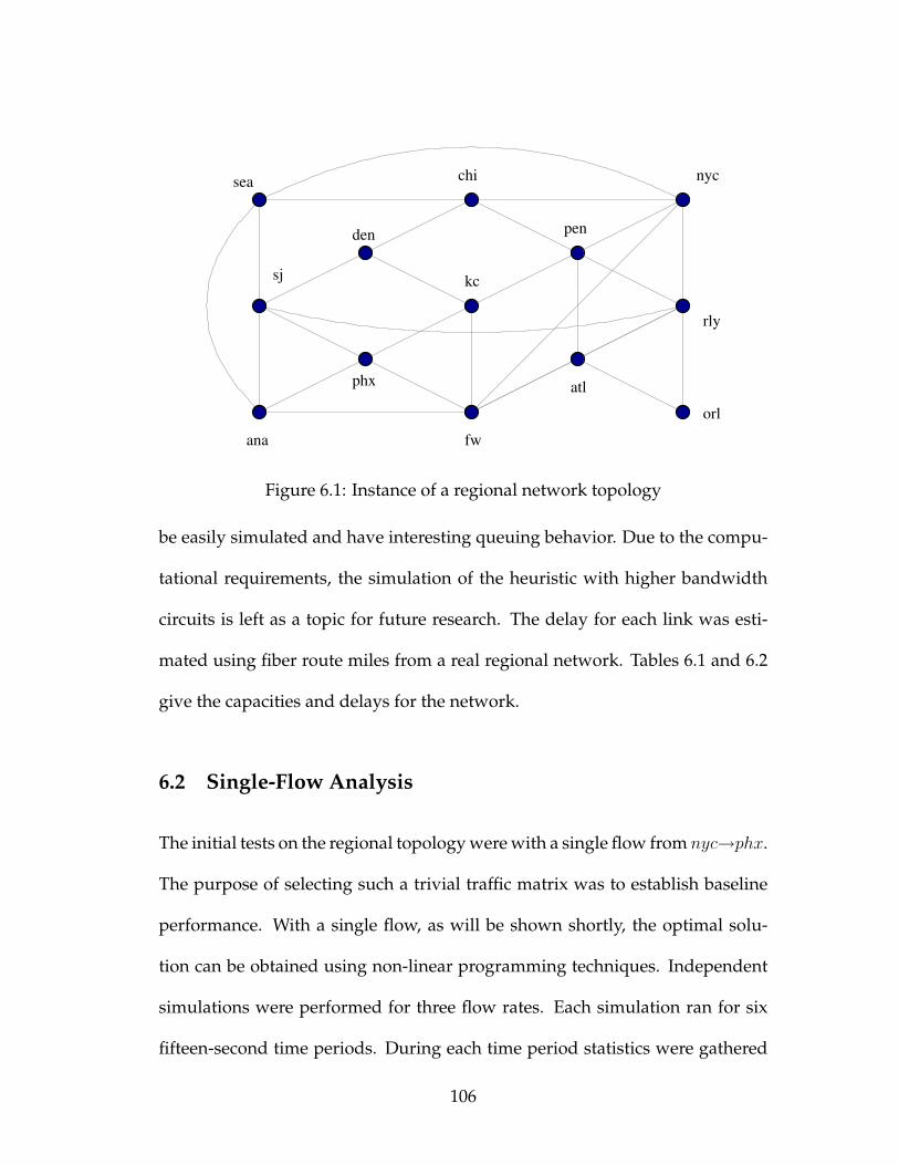
nyc
kc
den
sj
pen
fwana
rly
sea chi
atl
orl
phx
Figure 6.1: Instance of a regional network topology
be easily simulated and have interesting queuing behavior. Due to the compu-
tational requirements, the simulation of the heuristic with higher bandwidth
circuits is left as a topic for future research. The delay for each link was esti-
mated using fiber route miles from a real regional network. Tables 6.1 and 6.2
give the capacities and delays for the network.
6.2 Single-Flow Analysis
The initial tests on the regional topology were with a single flow from nyc→phx.
The purpose of selecting such a trivial traffic matrix was to establish baseline
performance. With a single flow, as will be shown shortly, the optimal solu-
tion can be obtained using non-linear programming techniques. Independent
simulations were performed for three flow rates. Each simulation ran for six
fifteen-second time periods. During each time period statistics were gathered
106

srcana atl chi den fw kc nyc orl pen phx wdc sea sj
ana · · · · 11 · · · · 3 · 13 4atl · · · · 8 · · 6 8 · 7 · ·chi · · · 8 · · 9 · 8 · · 19 ·den · · 8 · · 6 · · · · · · 12fw 11 8 · · · 5 16 · · 9 · · ·kc · · · 6 5 · · · 12 13 · · ·nyc · · 9 · 16 · · · 2 · 2 27 ·orl · 6 · · · · · · · · 10 · ·pen · 8 8 · · 12 2 · · · 2 · ·phx 3 · · · 9 13 · · · · · · 6wdc · 7 · · · · 2 10 2 · · · 27sea 13 · 19 · · · 27 · · · · · 10sj 4 · · 12 · · · · · 6 27 10 ·
Table 6.1: Regional network delay matrix (in ms)
srcana atl chi den fw kc nyc orl pen phx wdc sea sj
ana · · · · 30 · · · · 10 · 40 45atl · · · · 30 · · 10 15 · 20 · ·chi · · · 25 · · 20 · 40 · · 15 ·den · · 25 · · 20 · · · · · · 15fw 30 30 · · · 15 25 · · 15 · · ·kc · · · 20 15 · · · 15 40 · · ·nyc · · 20 · 25 · · · 40 · 40 40 ·orl · 10 · · · · · · · · 10 · ·pen · 15 40 · · 15 40 · · · 30 · ·phx 10 · · · 15 40 · · · · · · 20wdc · 20 · · · · 40 10 30 · · · 10sea 40 · 15 · · · 40 · · · · · 20sj 45 · · 15 · · · · · 20 10 20 ·
Table 6.2: Regional network capacity matrix (in Mb/s)
107

and reported. The state of the system was carried from one iteration into the
next, but not between simulations. The first flow rate was chosen to be small
enough to fit the entire flow on the shortest-delay path. The second flow rate
required the flow to be distributed between a few paths. The final flow rate
required the flow to be distributed across most of the available paths between
the source and the destination. Each flow-rate is discussed in its own section
below.
6.2.1 Small Flow
The best path between nyc and phx is nyc→fw→phx. The capacity on nyc→fw
is 25 Mb/s and the delay is 16 ms. On fw→phx the capacity is 15 Mb/s and
the delay is 9 ms. In order to accurately calculate the optimal average delay,
the queuing delay must be accounted for. Assuming the system is m/m/1, the
queuing delay for node x’s queue facing node y is
k
Cxy − Uxy(6.1)
where Cxy is the capacity of the link from node x to node y, Uxy is the total
amount of traffic from node x to node y in Mb/s, and k is a constant: the av-
erage packet size in bits. The expected average delay is the sum of the prop-
agation delays on the nyc→fw and fw→phx links and the associated queuing
delays: 25.85 ms.
The first segment in the path, nyc→fw, has a capacity of 25 Mb/s and the
second segment, fw→nyc, has a capacity of 15 Mb/s. The maximum flow size
that can be accommodated by the path is the minimum of these two: 15 Mb/s.
108

The initial flow size was chosen to be 10 Mb/s to ensure the entire flow can
fit on the shortest-delay path. Therefore, it is expected that the results for the
shortest-path approach will be near optimal.
The delay results for the nyc→phx 10 Mb/s flow are are shown in Figure 6.2.
The packet loss statistics can be found in Table 6.3. In each of these, opt refers
to the optimal solution, gd is the delay-aware heuristic, ga is the delay-agnostic
heuristic and spf is the shortest-path protocol.
1 2 3 4 5 6
iteration
aver
age
dela
y (m
s)
05
1015
2025
30
opt gd ga spf
Figure 6.2: Average delay for 10 Mb/s nyc→phx flow
iteration1 2 3 4 5 6
opt 0.0000 0.0000 0.0000 0.0000 0.0000 0.0000gd 0.0028 0.0000 0.0000 0.0000 0.0000 0.0000ga 0.0029 0.0000 0.0000 0.0000 0.0000 0.0000
spf 0.0000 0.0000 0.0000 0.0000 0.0000 0.0000
Table 6.3: Packet loss for 10 Mb/s nyc→phx flow
109

The average delay and loss for the shortest-path approach matched the op-
timal delay without experiencing any packet loss. The heuristic approaches,
while not perfect, found reasonable solutions. Each variation of the heuristic
was able to adapt within the first fifteen-second interval such that no packet
loss was experienced during subsequent intervals. The percentage of packets
lost during the first interval was under .3% for both approaches.
The delay-agnostic variation of the heuristic converged on a loss-free solu-
tion during the first fifteen-second interval and did not adapt further during the
subsequent intervals. The average delay during the final interval was within
20% of the optimal delay.
The delay-aware variation of the heuristic also converged on a loss-free so-
lution during the first fifteen-second interval. It continued to improve in terms
of delay during the second interval. The remaining four intervals saw little
change. During the final interval the average delay experienced by packets in
the network was within 1% of the optimal solution.
While both heuristic solutions were acceptable in terms of loss, the delay-
aware solution was clearly superior in terms of delay. This heuristic approach
was able to get reasonably close to the optimal solution without having any
foreknowledge of the topology, its delays and capacities, or the flows in the
network.
110

6.2.2 Medium Flow
A larger flow was used to study the ability of the heuristic to discover sec-
ondary routes when the flow size exceeds the capacity of the shortest-delay
path. Since the shortest-delay path from nyc to phx can only carry 15 Mb/s, a 25
Mb/s flow was selected for this trial, thus requiring some traffic to be placed on
an alternate path. The optimal solution for the 25 Mb/s flow can be estimated
by assuming just under 15 Mb/s will be sent on the shortest-delay path. After
subtracting 15 Mb/s of capacity from each of the two links in the shortest-delay
path, the second-best path can be found using a standard shortest-path algo-
rithm. The second-best path is found to be nyc→pen→kc→phx. Since this path
has a maximum capacity of 15 Mb/s (pen→kc link is the constraining link) it
will be able to carry the remainder of the flow. The average delay in the system
will be the weighted average of the delays associated with each path. To esti-
mate the optimal delay, assign 13 Mb/s to the shortest-delay path and 12 Mb/s
to the second best path. This results in an average delay of 27.6 ms.
A more accurate estimate of the optimal delay can be found by mathemat-
ically modeling the system as a series of equations and using non-linear pro-
gramming (NLP) techniques to find the minimal average delay. The equations
can be derived as follows. The average delay for a flow from node s destined
for node d is the weighted average of the delays associated with sending traffic
destined for d to each of the neighbors of node s. The weighting factor for each
egress link is the percentage of traffic destined for d sent on that egress link.
111

The delay associated with each neighbor is the sum of the amount of time to
get the traffic to that neighbor and that neighbor’s average delay to the destina-
tion. The amount of time required to get a packet to each neighbor is the sum of
the propagation and queuing delays, as described previously. The amount of
delay associated with a neighbor is a function of that neighbor’s own routing
table and the amount of traffic it is receiving.
For the current problem, the average delay for the flow f from nyc to phx
can be expressed as
Df,nyc = Pf,nyc,pen[dnyc,pen +k
Cnyc,pen − Unyc,pen+Df,pen]
+ Pf,nyc,fw[dnyc,fw +k
Cnyc,fw − Unyc,fw+Df,fw]
+ Pf,nyc,chi[dnyc,chi +k
Cnyc,chi − Unyc,chi+Df,chi]
+ Pf,nyc,wdc[dnyc,wdc +k
Cnyc,wdc − Unyc,wdc+Df,wdc]
+ Pf,nyc,sea[dnyc,sea +k
Cnyc,sea − Unyc,sea+Df,sea] (6.2)
where Pf,nyc,pen is the probability of traffic associated with flow f on node nyc
being sent toward pen, dnyc,pen is the propagation delay for the link between nyc
and pen, Cnyc,pen is the capacity between nyc and pen, k is the average packet
size in bits, Unyc,pen is the total utilization (in bits/second) of the nyc→pen link,
and Df,pen is the average delay from pen to the destination of flow f . The gen-
eralized form is
Df,a =∑
b∈fs(a)
Pf,a,b[da,b +k
Ca,b − Ua,b+Df,b] (6.3)
112
where fs(a) is the forward star of node a. In order to create a solvable system of
equations some additional supporting equations are required. First, the egress
interface selection probabilities on each node a for each flow f must sum to
one.
1 =∑
b∈fs(a)
Pf,a,b ∀a 6= (s, d) (6.4)
Next, a variable is defined representing the amount of traffic associated with
flow f leaving each node a: Tf,a. For all nodes that are not the source or the
destination of the flow, Tf,a can be represented as the sum of all traffic associ-
ated with the flow f entering the node due to the conservation of flow:
Tf,a =∑
b∈bs(a)
Pf,b,aTf,b (6.5)
where bs(a) is the backward star of a. Two boundary conditions can be defined
for the source and destination of flow, s and d:
Tf,s = |f | (6.6)
Tf,d = 0 (6.7)
where |f | is the size of the flow. These two equations simply state that the entire
flow leaves the source node and none of the flow leaves the destination node.
Finally, Ua,b, the utilization of the link from node a to node b can be defined in
terms of T :
Ua,b =∑f∈F
Pf,a,bTf,a (6.8)
where F is the set of all flows.
113

Using this set of equations and an NLP solver, the optimal delay for a single
25 Mb/s flow from nyc→phx is found to be 27.5. The estimated value was 27.6.
The solution found by the NLP solver may only be a local minimum. Having
the estimate available is valuable in gaining confidence in the solution. The
optimal solution found by the NLP solver represents a high-confidence guess
at what the minimum delay for the system really is.
Figure 6.3 shows the average delay over the six iterations for each of the
simulated algorithms. Table 6.4 provides the loss statistics measured by the
simulator.
1 2 3 4 5 6
iteration
aver
age
dela
y (m
s)
010
2030
4050
382.
18
370.
07
405.
65
379.
99
406.
18
377.
9
opt gd ga spf
Figure 6.3: Average delay for 25 Mb/s nyc→phx flow
The shortest-path approach performed poorly both in terms of delay and
loss as the capacity along the shortest-delay path was exceeded. Setting the
metrics to be something other than the propagation delay would have allowed
a better distribution of traffic across multiple paths. Finding the optimal met-
114
iteration1 2 3 4 5 6
opt 0.0000 0.0000 0.0000 0.0000 0.0000 0.0000gd 0.0012 0.0000 0.0000 0.0000 0.0000 0.0000ga 0.0015 0.0000 0.0000 0.0000 0.0000 0.0000
spf 0.3864 0.3852 0.3866 0.3856 0.3867 0.3865
Table 6.4: Packet loss for 25 Mb/s nyc→phx flow
rics, especially when the network has multiple flows, can be difficult if not
impossible. For the purposes of this comparison no attempt is made at such an
optimization. The extremely large delay is a result of full output queues along
the shortest-delay path.
The heuristic approaches performed considerably better. Regarding the pri-
mary objective, to minimize loss, both heuristic approaches were able to con-
verge on a loss-free solution within this fifteen-second interval. During the
first interval both variations of the heuristic approach experienced less than
.2% packet loss.
In terms of delay, the delay-aware variation of the heuristic was able to find a
superior solution to that found by the delay-agnostic variation. During the first
interval both approaches were roughly equal, but during the subsequent inter-
vals the delay-aware heuristic showed continuous improvement, resulting in a
solution that was within 1.5% of the optimal solution, while the solution found
by the delay-agnostic heuristic was only 20% of the optimal solution. Again,
as the delay-agnostic variation of the heuristic makes no effort to optimize in
terms of delay, these results are expected.
115

6.2.3 Large Flow
The final test using a single flow was performed with a 75 Mb/s nyc→phx
flow. This flow was large enough to require the use of numerous paths through
the network, including paths that made use of all four ingress links toward
phx. The optimal solution can be found using the same technique described in
Section 6.2.2 and an NLP solver. The minimum average delay was found to be
33.6 ms.
Figure 6.4 shows the average delay over the six iterations for each of the sim-
ulated routing approaches and Figure 6.5 shows the loss over the same period.
Tables 6.5 and 6.6 show the delay and loss measured by the simulator.
1 2 3 4 5 6
iteration
aver
age
dela
y (m
s)
020
4060
8010
012
0
681.
92
681.
86
681.
92
682.
26
682.
17
682.
05
opt gd ga spf
Figure 6.4: Average delay for 75 Mb/s nyc→phx flow
As with the 25 Mb/s flow, the shortest-path approach worked poorly both
in terms of average delay and packet loss. Unlike the 25 Mb/s flow, there is
116

iteration1 2 3 4 5 6
opt 33.60 33.60 33.60 33.60 33.60 33.60gd 54.23 44.51 42.44 45.43 39.65 39.56ga 111.99 116.58 111.44 112.98 95.99 39.16
spf 681.92 681.86 681.92 682.26 682.17 682.05
Table 6.5: Average delay for 75 Mb/s nyc→phx flow
1 2 3 4 5 6
iteration
pack
et lo
ss
0.00
00.
005
0.01
00.
015
0.02
0
0.79
08
0.79
15
0.79
11
0.79
05
0.79
14
0.79
05
opt gd ga spf
Figure 6.5: Packet loss for 75 Mb/s nyc→phx flow
iteration1 2 3 4 5 6
opt 0.0000 0.0000 0.0000 0.0000 0.0000 0.0000gd 0.0005 0.0000 0.0000 0.0000 0.0000 0.0000ga 0.0019 0.0005 0.0002 0.0002 0.0000 0.0000
spf 0.7908 0.7915 0.7911 0.7905 0.7914 0.7905
Table 6.6: Packet loss for 75 Mb/s nyc→phx flow
117

no apparent equal-cost load-balancing solution for the 75 Mb/s flow because
the smallest ingress link into phx is 10 Mb/s. Therefore, if each of the ingress
interfaces were to be used equally, at most 40 Mb/s of flow could be accom-
modated. Depending on the implementation of equal-cost load balancing of
the shortest-path algorithm, one could potentially have more than four equal-
cost paths from the perspective of nyc where some of these paths had the same
ingress link into phx. Finding such a solution is beyond the scope of this work.
In terms of loss, the delay-aware variation of the heuristic performed better
than the delay-agnostic version. While both were able to keep the packet loss
well under 1%, the delay-aware variation did not experience any loss after the
first iteration. The delay-agnostic version experienced small amounts of loss
during the first four iterations.
In addition to higher loss, the delay-agnostic version also struggled during
the first four iterations to find a solution with good delay characteristics. Dur-
ing the first four iterations the average delay for this version of the heuristic
was over 100 ms. Surprisingly, during the sixth iteration it found a solution
that was superior in terms of delay to that found by the delay-aware version.
Both solutions at this point were a little less than 20% from the optimal solution.
For both versions the simulation was allowed to continue for 10 additional
iterations, representing a composite simulation time of about 4 minutes. Over
these iterations the average delay did not significantly change, with the delay-
aware heuristic averaging 40 ms and the delay-agnostic version averaging 38
ms. These results are consistent with the behavior observed on the heavily
118

loaded ring network studied in the previous chapter and indicate a stable con-
vergence.
6.3 Multiple Flows
The purpose of this section is to study the behavior of the heuristic in the pres-
ence of a small number of independent flows competing for network resources.
Four separate experiments were performed, each adding one or more flows to
the previously studied nyc→phx 25 Mb/s flow. Each trial is discussed in its
own section below.
6.3.1 Adding a Flow from fw→phx
Section 6.2.2 deals with a single nyc→phx 25 Mb/s flow. The optimal path
for flow distributes the data nearly equally between the nyc→fw→phx and
nyc→pen→kc→phx paths. For this trial an additional flow is included that
sources traffic at fw destined for phx. With the introduction of this flow there is
insufficient capacity on the fw→phx link for both flows. Therefore, each flow
will need some of its traffic to be distributed on secondary and tertiary paths.
Using previously defined equations and an NLP solver, the minimum average
delay in the network is found to be 24.06 ms.
Figures 6.6 and 6.7 show the average delay and packet loss over the six it-
erations for each of the simulated algorithms. Tables 6.7 and 6.8 provide the
specific values measured by the simulator.
119

1 2 3 4 5 6
iteration
aver
age
dela
y (m
s)
010
2030
4050
370.
04
361.
6
355.
55
378.
84
360.
64
360.
59
opt gd ga spf
Figure 6.6: Average delay for 25 Mb/s nyc→phx flow and 10 Mb/s fw→phxflow
iteration1 2 3 4 5 6
opt 24.06 24.06 24.06 24.06 24.06 24.06gd 30.93 26.66 26.62 26.71 26.30 26.30ga 32.11 28.21 28.19 28.21 28.15 28.20
spf 370.04 361.60 355.55 378.84 360.64 360.59
Table 6.7: Average delay for 25 Mb/s nyc→phx flow and 10 Mb/s fw→phxflow
iteration1 2 3 4 5 6
opt 0.0000 0.0000 0.0000 0.0000 0.0000 0.0000gd 0.0007 0.0000 0.0000 0.0000 0.0000 0.0000ga 0.0008 0.0000 0.0000 0.0000 0.0000 0.0000
spf 0.5600 0.5590 0.5585 0.5623 0.5600 0.5610
Table 6.8: Packet loss for 25 Mb/s nyc→phx flow and 10 Mb/s fw→phx flow
120
1 2 3 4 5 6
iteration
pack
et lo
ss
0.00
00.
005
0.01
00.
015
0.02
0
0.56
0.55
9
0.55
85
0.56
23 0.56
0.56
1
opt gd ga spf
Figure 6.7: Packet loss for 25 Mb/s nyc→phx flow and 10 Mb/s fw→phx flow
Consistent with the observations in Section 6.2.2, the shortest-path approach
performed poorly. Both heuristic approaches converged on loss-free solutions
during the first fifteen-second interval. During this interval the packet loss for
both approaches was well under 1%.
In terms of delay, both versions of the heuristic converged on a stable so-
lution during the second interval, with the delay-aware heuristic performing
slightly better than the delay-agnostic version. The delay-agnostic version found
a solution within 20% of the optimal solution while the delay-aware heuristic
converged on a solution within 10% of the optimal solution.
6.3.2 Adding a Flow from pen→kc
In the previous section the second flow had a common endpoint with the first
flow. This section explores the effect of adding a second flow that does not
121

have an endpoint in common with the nyc→phx flow but does share a commu-
nications link in the optimal solutions. The flow chosen for this analysis is a 10
Mb/s flow from pen to kc. The nyc→phx flow needs to use this link as part of its
second-best path, but with the additional traffic from the new flow an alternate
route will need to be discovered.
Figures 6.8 and 6.9 show the average delay and packet loss over the six it-
erations for each of the simulated algorithms. Tables 6.9 and 6.10 provide the
specific values measured by the simulator.
1 2 3 4 5 6
iteration
aver
age
dela
y (m
s)
010
2030
4050
237.
95
243.
37
260.
11
238.
68
262.
8
251.
31
opt gd ga spf
Figure 6.8: Average delay for 25 Mb/s nyc→phx flow and 10 Mb/s pen→kcflow
Both heuristic approaches were again able to find loss-free routing solutions
during the first fifteen-second interval, and during this first interval both ap-
proaches experienced well under 1% loss.
122

iteration1 2 3 4 5 6
opt 24.53 24.53 24.53 24.53 24.53 24.53gd 28.73 27.82 26.99 27.09 27 27.12ga 28.17 26.92 26.97 27.01 27.07 27.17
spf 237.95 243.37 260.11 238.68 262.80 251.31
Table 6.9: Average delay for 25 Mb/s nyc→phx flow and 10 Mb/s pen→kc flow
1 2 3 4 5 6
iteration
pack
et lo
ss
0.00
00.
005
0.01
00.
015
0.02
0
0.27
52
0.27
47
0.27
46
0.27
43
0.27
63
0.27
6
opt gd ga spf
Figure 6.9: Packet loss for 25 Mb/s nyc→phx flow and 10 Mb/s pen→kc flow
iteration1 2 3 4 5 6
opt 0.0000 0.0000 0.0000 0.0000 0.0000 0.0000gd 0.0013 0.0000 0.0000 0.0000 0.0000 0.0000ga 0.0015 0.0000 0.0000 0.0000 0.0000 0.0000
spf 0.2752 0.2747 0.2746 0.2743 0.2763 0.2760
Table 6.10: Packet loss for 25 Mb/s nyc→phx flow and 10 Mb/s pen→kc flow
123

In terms of delay, both heuristic approaches were roughly equal with solu-
tions within 11% of the delay expected from the optimal solution. As the delay-
agnostic heuristic focuses on finding any solution not having packet loss, it is
reasonable that occasionally it will find a similar solution to the delay-aware
version, providing that solution does not have packet loss.
6.3.3 Adding a Flow from fw→phx and from pen→kc
In this section both of the flows added in the previous two sections are added
at the same time to the 25 Mb/s nyc→phx flow. The minimum average delay
with this environment is calculated to be 23.05 ms.
Figures 6.10 and 6.11 show the average delay and packet loss over the six
iterations for each of the simulated algorithms. Tables 6.11 and 6.12 provide
the specific values measured by the simulator.
iteration1 2 3 4 5 6
opt 23.05 23.05 23.05 23.05 23.05 23.05gd 30.51 26.33 26.82 26.49 25.95 25.17ga 31.19 26.26 26.29 26.37 26.37 26.42
spf 246.66 251.17 250.60 265.06 253.07 263.23
Table 6.11: Average delay for 25 Mb/s nyc→phx flow, 10 Mb/s pen→kc flow,and 10 Mb/s fw→phx flow
As before, the packet loss stayed well below 1% and went to zero after
the first fifteen-second interval. The average delay associated with the delay-
agnostic version was within 15% of the optimal delay while the delay-aware
version was able to achieve an average delay within 10% of optimal.
124
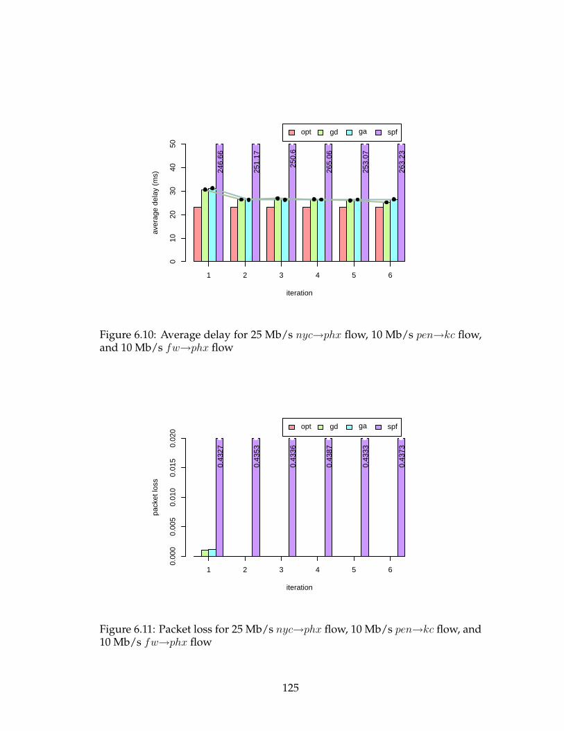
1 2 3 4 5 6
iteration
aver
age
dela
y (m
s)
010
2030
4050
246.
66
251.
17
250.
6
265.
06
253.
07
263.
23
opt gd ga spf
Figure 6.10: Average delay for 25 Mb/s nyc→phx flow, 10 Mb/s pen→kc flow,and 10 Mb/s fw→phx flow
1 2 3 4 5 6
iteration
pack
et lo
ss
0.00
00.
005
0.01
00.
015
0.02
0
0.43
27
0.43
53
0.43
36
0.43
87
0.43
33
0.43
73
opt gd ga spf
Figure 6.11: Packet loss for 25 Mb/s nyc→phx flow, 10 Mb/s pen→kc flow, and10 Mb/s fw→phx flow
125
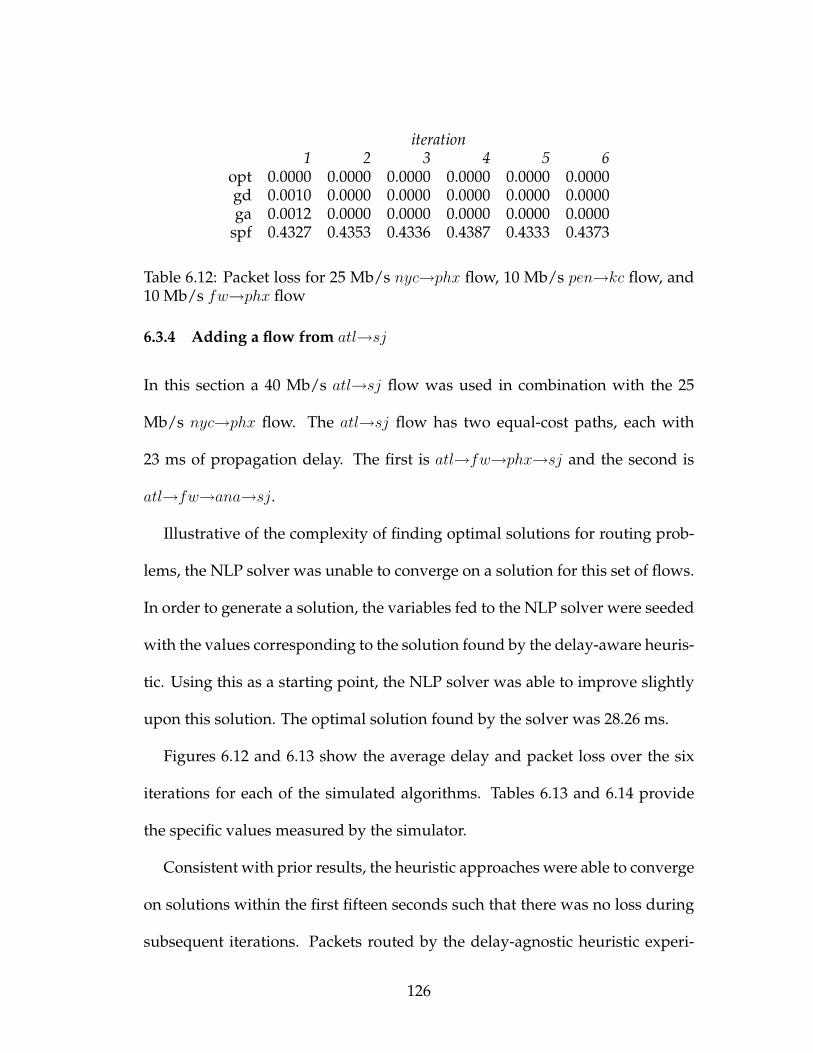
iteration1 2 3 4 5 6
opt 0.0000 0.0000 0.0000 0.0000 0.0000 0.0000gd 0.0010 0.0000 0.0000 0.0000 0.0000 0.0000ga 0.0012 0.0000 0.0000 0.0000 0.0000 0.0000
spf 0.4327 0.4353 0.4336 0.4387 0.4333 0.4373
Table 6.12: Packet loss for 25 Mb/s nyc→phx flow, 10 Mb/s pen→kc flow, and10 Mb/s fw→phx flow
6.3.4 Adding a flow from atl→sj
In this section a 40 Mb/s atl→sj flow was used in combination with the 25
Mb/s nyc→phx flow. The atl→sj flow has two equal-cost paths, each with
23 ms of propagation delay. The first is atl→fw→phx→sj and the second is
atl→fw→ana→sj.
Illustrative of the complexity of finding optimal solutions for routing prob-
lems, the NLP solver was unable to converge on a solution for this set of flows.
In order to generate a solution, the variables fed to the NLP solver were seeded
with the values corresponding to the solution found by the delay-aware heuris-
tic. Using this as a starting point, the NLP solver was able to improve slightly
upon this solution. The optimal solution found by the solver was 28.26 ms.
Figures 6.12 and 6.13 show the average delay and packet loss over the six
iterations for each of the simulated algorithms. Tables 6.13 and 6.14 provide
the specific values measured by the simulator.
Consistent with prior results, the heuristic approaches were able to converge
on solutions within the first fifteen seconds such that there was no loss during
subsequent iterations. Packets routed by the delay-agnostic heuristic experi-
126

1 2 3 4 5 6
iteration
aver
age
dela
y (m
s)
010
2030
4050
443.
47
447.
03
437.
54
444.
56
439.
21
449.
72
opt gd ga spf
Figure 6.12: Average delay for 25 Mb/s nyc→phx flow and 40 Mb/s pen→kcflow
iteration1 2 3 4 5 6
opt 28.26 28.26 28.26 28.26 28.26 28.26gd 35.13 29.86 29.4 28.75 28.96 28.95ga 37.05 32.96 32.91 32.97 33.01 33.08
spf 443.47 447.03 437.54 444.56 439.21 449.72
Table 6.13: Average delay for 25 Mb/s nyc→phx flow and 40 Mb/s pen→kcflow
iteration1 2 3 4 5 6
opt 0.0000 0.0000 0.0000 0.0000 0.0000 0.0000gd 0.0009 0.0000 0.0000 0.0000 0.0000 0.0000ga 0.0009 0.0000 0.0000 0.0000 0.0000 0.0000
spf 0.5235 0.5216 0.5221 0.5226 0.5239 0.5248
Table 6.14: Packet loss for 25 Mb/s nyc→phx flow and 40 Mb/s pen→kc flow
127

1 2 3 4 5 6
iteration
pack
et lo
ss
0.00
00.
005
0.01
00.
015
0.02
0
0.52
35
0.52
16
0.52
21
0.52
26
0.52
39
0.52
48
opt gd ga spf
Figure 6.13: Packet loss for 25 Mb/s nyc→phx flow and 40 Mb/s pen→kc flow
enced an average delay of 33 ms during the final interval, 17% greater than the
minimum delay. The delay-aware version did better, with an average delay
that was only 2.5% greater than the minumum delay found by the NLP solver.
6.4 All-Pairs Flows
The final simulation with the regional network includes flows between every
pair of routers. Finding the optimal flow distribution for this problem is unrea-
sonable using standard computing hardware, as the system to optimize is over
6000 equations with more than 12000 variables. To ensure the heuristic could
be compared to something meaningful, the flow sizes were chosen to be small
enough that each flow could fit on its shortest-delay path. Because of this, the
shortest-path algorithm will find the optimal solution.
128

Figures 6.14 and 6.15 show the average delay and packet loss over the six
iterations for each of the simulated algorithms. Tables 6.15 and 6.16 provide
the specific values measured by the simulator.
1 2 3 4 5 6
iteration
aver
age
dela
y (m
s)
05
1015
2025
opt gd ga spf
Figure 6.14: Average delay for flows between every pair of nodes in the net-work
iteration1 2 3 4 5 6
opt 17.32 17.32 17.32 17.32 17.32 17.32gd 25.20 19.39 18.84 18.49 18.25 18.06ga 25.69 20.48 20.24 20.16 20.09 20.07
spf 17.33 17.33 17.31 17.32 17.32 17.34
Table 6.15: Average delay for flows between every pair of nodes in the network
Once again the heuristic approaches were able to meet their primary objec-
tive, avoiding loss. After the first fifteen-second interval neither variation of the
heuristic dropped a single packet. In terms of delay, the delay-agnostic varia-
tion found a solution after six iterations which was within 16% of the optimal
129

1 2 3 4 5 6
iteration
pack
et lo
ss
0.00
000.
0005
0.00
100.
0015
0.00
20opt gd ga spf
Figure 6.15: Packet loss for flows between every pair of nodes in the network
iteration1 2 3 4 5 6
opt 0.0000 0.0000 0.0000 0.0000 0.0000 0.0000gd 0.0020 0.0000 0.0000 0.0000 0.0000 0.0000ga 0.0019 0.0000 0.0000 0.0000 0.0000 0.0000
spf 0.0000 0.0000 0.0000 0.0000 0.0000 0.0000
Table 6.16: Packet loss for flows between every pair of nodes in the network
130
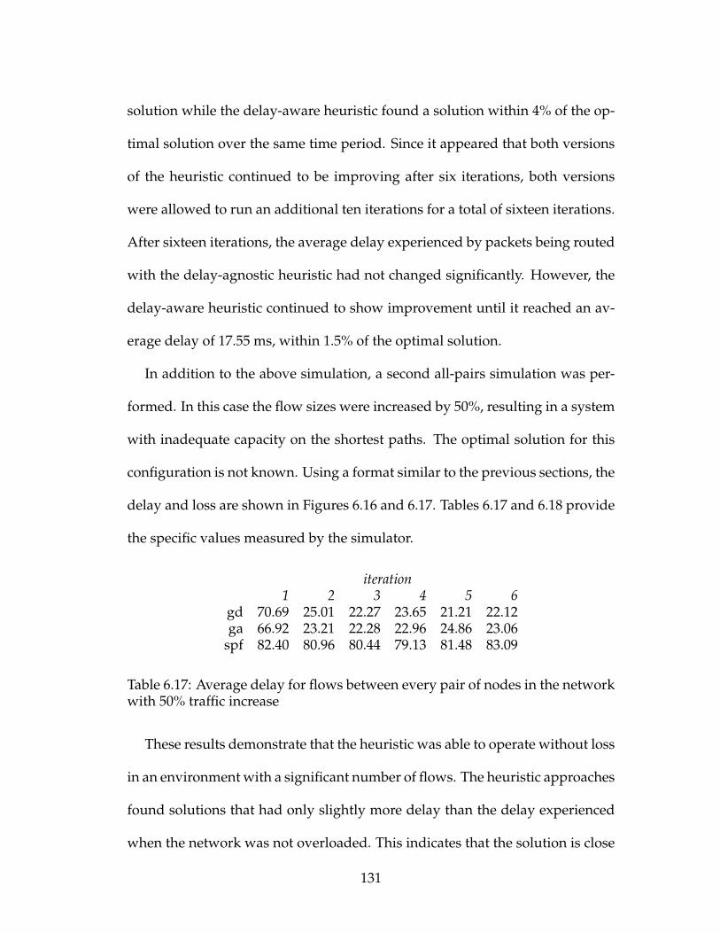
solution while the delay-aware heuristic found a solution within 4% of the op-
timal solution over the same time period. Since it appeared that both versions
of the heuristic continued to be improving after six iterations, both versions
were allowed to run an additional ten iterations for a total of sixteen iterations.
After sixteen iterations, the average delay experienced by packets being routed
with the delay-agnostic heuristic had not changed significantly. However, the
delay-aware heuristic continued to show improvement until it reached an av-
erage delay of 17.55 ms, within 1.5% of the optimal solution.
In addition to the above simulation, a second all-pairs simulation was per-
formed. In this case the flow sizes were increased by 50%, resulting in a system
with inadequate capacity on the shortest paths. The optimal solution for this
configuration is not known. Using a format similar to the previous sections, the
delay and loss are shown in Figures 6.16 and 6.17. Tables 6.17 and 6.18 provide
the specific values measured by the simulator.
iteration1 2 3 4 5 6
gd 70.69 25.01 22.27 23.65 21.21 22.12ga 66.92 23.21 22.28 22.96 24.86 23.06
spf 82.40 80.96 80.44 79.13 81.48 83.09
Table 6.17: Average delay for flows between every pair of nodes in the networkwith 50% traffic increase
These results demonstrate that the heuristic was able to operate without loss
in an environment with a significant number of flows. The heuristic approaches
found solutions that had only slightly more delay than the delay experienced
when the network was not overloaded. This indicates that the solution is close
131
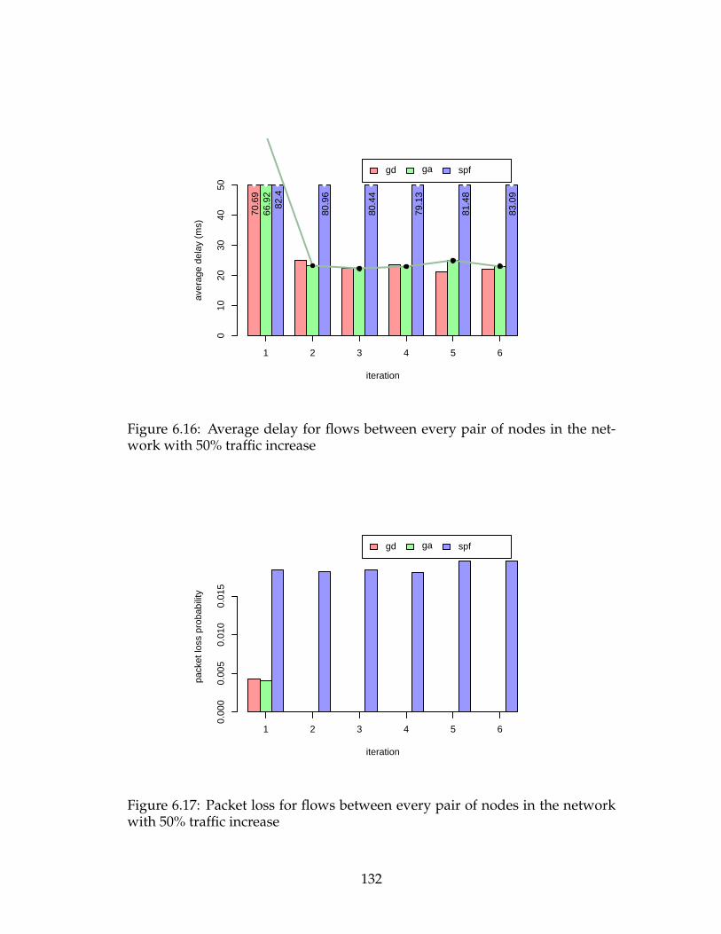
1 2 3 4 5 6
iteration
aver
age
dela
y (m
s)
010
2030
4050
70.6
966
.92
82.4
80.9
6
80.4
4
79.1
3
81.4
8
83.0
9
gd ga spf
Figure 6.16: Average delay for flows between every pair of nodes in the net-work with 50% traffic increase
1 2 3 4 5 6
iteration
pack
et lo
ss p
roba
bilit
y
0.00
00.
005
0.01
00.
015
gd ga spf
Figure 6.17: Packet loss for flows between every pair of nodes in the networkwith 50% traffic increase
132

iteration1 2 3 4 5 6
gd 0.0043 0.0000 0.0000 0.0000 0.0000 0.0000ga 0.0040 0.0000 0.0000 0.0000 0.0000 0.0000
spf 0.0184 0.0182 0.0184 0.0181 0.0195 0.0195
Table 6.18: Packet loss for flows between every pair of nodes in the networkwith 50% traffic increase
to optimal, as the average delay of the optimal solution with increased traffic
will be slightly larger than the average delay prior to the flow-size increase. The
large increase in delay experienced by the shortest-path approach indicates that
many flows were being routed over congested paths.
6.5 Chapter Summary
This chapter has demonstrated that in the regional network studied, the pro-
posed heuristic is able to meet its primary objective of avoiding loss. In ad-
dition, the delay-aware variation of the heuristic is shown to outperform the
delay-agnostic variation. A summary of the relative performance for both vari-
ations of the genetic heuristic is shown in Table 6.19.
In every trial, the heuristic approaches were able to find a loss-free solution
during the first fifteen-second interval. In addition, the loss during the first in-
terval never exceeded 1%. It might seem counter-intuitive that the delay-aware
heuristic was able to consistently out-perform the delay-agnostic heuristic in
terms of loss. However, this can be explained. The delay-agnostic variation’s
first indication of congestion is when the congestion is severe enough to cause
133
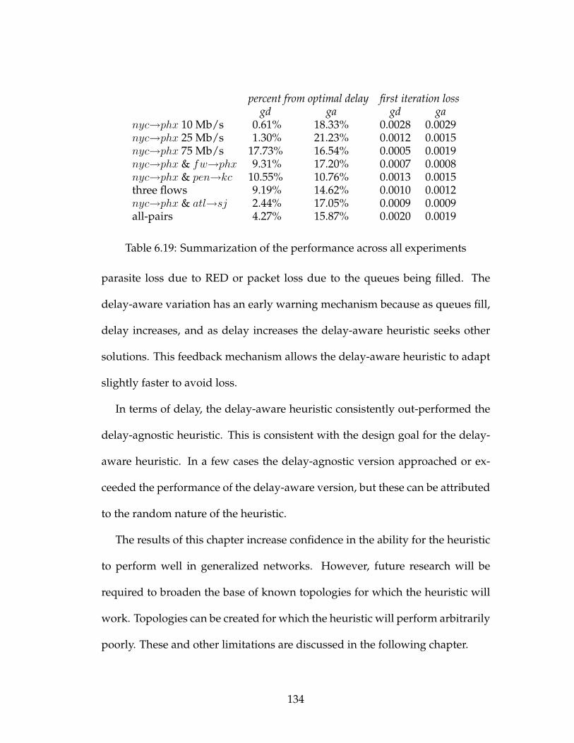
percent from optimal delay first iteration lossgd ga gd ga
nyc→phx 10 Mb/s 0.61% 18.33% 0.0028 0.0029nyc→phx 25 Mb/s 1.30% 21.23% 0.0012 0.0015nyc→phx 75 Mb/s 17.73% 16.54% 0.0005 0.0019nyc→phx & fw→phx 9.31% 17.20% 0.0007 0.0008nyc→phx & pen→kc 10.55% 10.76% 0.0013 0.0015three flows 9.19% 14.62% 0.0010 0.0012nyc→phx & atl→sj 2.44% 17.05% 0.0009 0.0009all-pairs 4.27% 15.87% 0.0020 0.0019
Table 6.19: Summarization of the performance across all experiments
parasite loss due to RED or packet loss due to the queues being filled. The
delay-aware variation has an early warning mechanism because as queues fill,
delay increases, and as delay increases the delay-aware heuristic seeks other
solutions. This feedback mechanism allows the delay-aware heuristic to adapt
slightly faster to avoid loss.
In terms of delay, the delay-aware heuristic consistently out-performed the
delay-agnostic heuristic. This is consistent with the design goal for the delay-
aware heuristic. In a few cases the delay-agnostic version approached or ex-
ceeded the performance of the delay-aware version, but these can be attributed
to the random nature of the heuristic.
The results of this chapter increase confidence in the ability for the heuristic
to perform well in generalized networks. However, future research will be
required to broaden the base of known topologies for which the heuristic will
work. Topologies can be created for which the heuristic will perform arbitrarily
poorly. These and other limitations are discussed in the following chapter.
134
Chapter 7
Challenges for the Heuristic
As might be expected, the proposed heuristic approach has limitations and
shortcomings. Many of these were anticipated and others were discovered in
the course of this research. The purpose of this chapter is to describe some of
the more significant shortcomings and limitations which impact the effective-
ness of the heuristic. While no insurmountable challenges were encountered
during the implementation of the heuristic, lessons were learned. These were
discussed in Chapter 8. This chapter focuses on non-implementation issues.
This chapter includes two sections: the first discusses topologies in which
the heuristic is expected to perform poorly and the second identifies many of
the challenges the heuristic would face if applied to routing on the Internet.
In both sections, mitigation strategies are proposed when available. While it
may be troubling to devote an entire chapter to the subject of the heuristic’s
limitations, understanding them is essential to determine where, how, and if
the heuristic might be applied to real-world routing problems.
135
7.1 General Network-Related Challenges
The heuristic has been shown to operate well for a relatively limited set of
topologies. It is possible to define topologies for which the heuristic can be
made to perform arbitrarily poorly.
Prior to converging on a routing solution, the heuristic method is roughly
equivalent to random routing[48]. Its ability to adapt and converge is based
on the assumption that some of the randomly routed packets eventually ar-
rive at their destinations. There are many ways to decrease the probability a
packet successfully reaches its destination. One approach would be to increase
the number of routing decisions that must be made (related to the diameter of
the network). Another would be to increase the number of “wrong” choices
available for each decision (related to the degree of the nodes on the network).
In addition, the time-to-live of packets being injected into the network greatly
affects the impact of the topology by limiting the number of routing mistakes
from which a packet can recover. All three of these may be combined to create
a system for which the heuristic would perform miserably. Understanding the
limitations is essential to identify the situations in which the heuristic should
not be used.
7.1.1 Time-to-Live of Packets
Prior to discussing the topological issues, it is important to understand the im-
pact of the time-to-live (TTL) field of packets being injected in the network.
136

Most network protocols incorporate some type of a time-to-live field into the
headers of packets being routed on the network. The purpose of this field is
to ensure that incorrectly routed packets do not loop indefinitely in the net-
work. For simplicity, this field typically does not measure time, but rather “hop
counts,” or the number of routers through which the packet has passed. The
system creating the packet sets the TTL and then each router along the path
decrements it by one. When the counter reaches zero the packet is assumed to
be looping and it is dropped.
By limiting the amount of time a packet can exist in the network, the TTL
field also limits the number of routing “mistakes” from which it can recover.
Given a generous setting for the TTL this should not be a problem, but it is
possible to set the TTL low enough to impact the ability for the heuristic to
learn. The proposed heuristic initially relies on discovering a feasible path by
following a random path to the destination. Depending upon the topology of
the network, the anticipated number of hops expected prior to reaching the
destination can be quite large[48]. By restricting the number of total hops, the
TTL might greatly increase the anticipated convergence time.
Consider the triplet network discussed in Chapter 4. The probability that a
packet injected at node 2 destined for node 3 with a TTL of 1 making it to its
destination is initially .5. If the TTL is increased to 3, the packet could survive
one routing mistake, increasing the probability of successful delivery to 1 −
.52 = .75. The TTL needs to increase by two to account for being decremented
both when it goes to node 1 and when node 1 returns it to node 2. Node 2 then
137
has a second chance to make a routing decision. In general, the probability of
successful delivery for a randomly routed packet is 1 − .5dn/2e where n is the
initial TTL of the injected packet at node 2. This demonstrates the negative
impact of a low TTL. While in this case the probability of successful delivery is
favorable, routing for most topologies is not this simple.
Mitigation strategies for TTL-related problems are limited to affecting how
the TTL is set initially and how the network operates on the field. The initial
TTL value typically is determined by the system originating the packet. This
system has the best chance of understanding of the importance of the packet
and the maximum distance it should need to travel. The first router to attach
a parasite could potentially increase the TTL of the packet, thus increasing the
likelihood of its eventual delivery. However, if the packet were to be passed
between routing domains, unbounded looping could result. A better strategy
might be for the routers to modify their drop logic to not drop a packet with
a TTL of zero when it is carrying parasites. Rather, an additional TTL field
could be added to the header of packets carrying parasites. This value could
be larger than the packet TTL, but still be small enough to keep packets from
looping indefinitely.
The TTL of packets affects the probability a routing error can be survived. In
the next two sections topology issues that affect the probability a routing error
will occur will be discussed.
138
7.1.2 High-Degree Nodes
The degree of a node in a network affects the probability that a randomly se-
lected egress link is on the desired path. In particular, if a node has only one
feasible exit, each additional exit represents an additional wrong choice to be
possibly made. In real-world networks, such nodes are common: local area net-
works (LANs) typically connect many hundreds of computers to one or more
routers. In large regional networks LANs are sometimes used in switch sites
for traffic aggregation. While extremely important to networking in general,
LANs are considered outside the domain of networks for which the proposed
heuristic has applicability.
Similarly, the degree of a node greatly affects the speed at which a new path
might be discovered once the heuristic has converged. The number of muta-
tions is equally divided among all egress links. Therefore, as the number of
egress links increases, the frequency at which each is probed for new solutions
decreases.
Balancing the negative impact of high-degree nodes is the reality that of-
ten the additional links are associated with additional paths to the destination.
Therefore, adding another egress interface does not necessarily increase the
probability a bad routing choice will be made. The above discussion made
the assumption that there was only one valid egress link for the destination.
If this assumption is not valid, and it often is not, then the negative impact of
high-degree nodes can be mitigated.
139

Of greater impact than node degree, however, is the diameter of the network.
The following section discusses its effect.
7.1.3 Network Diameter
The diameter of a network is the largest distance, in terms of hops, between any
pair of nodes. It directly impacts the probability that a randomly routed packet
will not exceed its TTL by defining the number of correct routing decisions
that are required. The probability of successfully routing a packet is the joint
probability that each step along the way correctly routes the packet.
Consider a 2n+1 node network where every node i, 1 < i < 2n, is connected
to node i+1. Assume packets destined for node 1 with a hop-based TTL of n−1
are entering the network at node n. For the packet to reach its destination, each
node i must send the packet to the adjacent node i − 1. If any node i in the
path makes the wrong choice and routes the packet toward node i + 1, the
packet ultimately will not reach its destination, as the TTL will reach zero prior
to its arrival at node 1. Assuming an initially random system, the probability
that a packet will reach its destination (and hence the chance of the system
learning anything useful) is .5n−1. For modest values of n the probability of a
packet reaching its destination are bleak. For example, if n = 14, approximately
one packet in ten thousand would make it. Node 2 would receive only a few
marked packets for every ten thousand packets sampled by node n. Eventually
the system would converge, but the requisite time would be measured in hours,
140

days, or years instead of seconds. The problem could be further exacerbated by
increasing the degree of nodes along the path.
Decreasing the impact of the network diameter is the reality that networks
often ingress traffic at all nodes, and the destinations of this traffic are typically
spread among the set of all routers in the network. Therefore, some of the
traffic will have short paths, allowing the routing to adapt from the inside out.
Consider again the topology for which initially only one out of many thousands
of packets would be successfully delivered. This time assume every node in
the network is receiving packets destined for node 1. The probability of node
2 randomly discovering the path to node 1 is .5. After some fixed number of
packets, node 2 will have converged on a good routing solution for node 1.
Assign T to be the amount of time node 2 required to adapt. At time T the
probability that packets ingressing on node 3 will make it to node 2 without
being sent toward node 4 is at worst .5. It will be even higher if node 3 was
able to learn during the interval in which node 2 converged. Node 3 should
then be able to converge in a similar time interval. Extending this to node n,
the expected convergence time is now nT , which is likely to be acceptable.
7.1.4 Summary of Network-Related Challenges
This section discussed some of the topologies for which the heuristic is ex-
pected to perform poorly. It likely that many additional topologies exist in
which the heuristic will not function well. An important question not answered
by this section is how often such topologies are expected to exist. Understand-
141

ing the impact the topological structure has on the heuristic is essential to un-
derstanding the plausibility of its application to a real-world problem.
7.2 Challenges Specific to IP Networks
The Internet’s success makes it a de facto target for most new routing protocols.
Because of its importance, any improvement in routing efficiency or reliabil-
ity could have a significant impact. Unfortunately, significant challenges are
related to routing in an internet protocol (IP) network using the heuristic as
proposed. Some of the limitations include the large number of possible desti-
nations, packet reordering, multicast, fragmentation, the space available in the
IP header, and the interaction with Border Gateway Protocol (BGP). Each of
these is discussed below along with potential solutions, when available.
7.2.1 Destinations
The current version of the Internet Protocol, IPv4[72], supports approximately
4 billion unique destination addresses. IPv6[23] supports many more. Main-
taining a population for each destination is challenging for many reasons. First,
the amount of memory required to store all of the populations is likely be pro-
hibitive. Second, convergence time is related to the number of packets being
sent toward a destination, and having one population for each end-system may
result in populations not having ample traffic to converge quickly. Finally, hav-
ing per-destination populations assumes that all routers in the network are par-
142
ticipants in the heuristic algorithm. In a network with as diverse control as the
Internet this assumption is unrealistic. For the heuristic to work with IPv4,
some form of address aggregation is required to create consistent groupings of
destination addresses that can share the same population. This will decrease
the amount of memory, combine traffic to allow for more rapid convergence,
and allow continued autonomous control of networking infrastructure.
The first opportunity for aggregation is to follow the aggregation present in
current route tables, as addresses are allocated in blocks and not individually.
In such an environment there would be a population corresponding to every
address block. This limits the number of populations to a few hundred thou-
sand initially. However, the amount of memory space required to maintain a
population is likely to be much larger than the amount of space used by the
standard route table.∗ For this reason additional aggregation is desirable.
A better approach is to aggregate all destination addresses associated with
the same egress edge-router. In the view of the heuristic, the egress edge-
router’s loopback address would be the “destination” of the packet instead of
the destination encoded into the packet header. Given that today’s largest net-
works typically have less than a few thousand routers, this approach greatly
reduces the number of populations required to be maintained on each router.
Such a model assumes that all routers in the network are capable of consis-
tently determining the egress edge-router for an address. This information
can be obtained from the continued use of external-gateway routing protocols
∗The size of the population will likely be a function of the number of egress links on the router.
143

such as BGP[77] to communicate external reachability information between au-
tonomous systems. Routers receiving BGP announcements from external peers
could set the next-hop to be their own loopback address. It is not clear, how-
ever, how the BGP information would be propagated within the network prior
to the heuristic’s convergence.
7.2.2 Packet Reordering
The heuristic proposed herein would likely cause significant packet reorder-
ing. The problem is especially pronounced when two or more egress links with
widely varied delay characteristics have significant representation in a popu-
lation. Nothing in the heuristic seeks to influence packets in the same flow to
use the same egress link. In fact, the heuristic maintains no awareness of flows,
and thus has no opportunity to ensure flows are routed consistently.
TCP is capable of dealing with out-of-order packet delivery. However, it has
been shown that massive packet reordering may result in profoundly degraded
performance which in some cases becomes self-reinforcing[5]. For this reason,
it is important to limit the amount of reordering that occurs in the network.
With traditional routing protocols, reordering typically results from routing
pathologies and, increasingly, local parallelism of communications links. How-
ever, the resultant reordering has thus far been manageable.
Fixing TCP to more efficiently process out-of-order packets is a potential
strategy to deal with the reordering introduced by the heuristic. One technique
that attempts to make TCP less susceptible to performance degradation in the
144

presence of reordering involves altering the packet acknowledgment strategy
to be more selective[57]. While such an approach holds promise, out-of-order
packets will continue to have some negative impact on performance and thus
should be avoided when possible.
The heuristic could be modified to maintain an awareness of flows and ac-
tively seek to send packets within a flow on the same egress. This approach
would likely address many of the reordering problems, but has the potential to
create others, as the adaptation of the populations would be affected by flow
characteristics. Large flows would tend to pull the population toward their
egress links. No attempt is made in this research to quantify this effect.
Some existing aspects of the heuristic may serve to dampen the negative
effects of reordering. In particular, reordering has less of an impact if the re-
ordered packets arrive relatively close together. The delay-aware variation of
the heuristic favors the lowest-delay path. If multiple paths are being used,
then these multiple paths likely have similar delay characteristics and, there-
fore, the impact of reordering should not be as significant.
In a network environment where in-order delivery is a significant require-
ment, the proposed heuristic is ill-suited. In more flexible environments where
out-of-order delivery can be tolerated, the packet reordering associated with
the heuristic may be acceptable.
145
7.2.3 Multicast
Multicast routing protocols build forwarding trees based on the reverse-path
forwarding (RPF) rule. This rule states if a packet is received on the interface
that would be used to forward a unicast packet back to the source of the packet,
then the packet is forwarded on all other interfaces that have downstream re-
ceivers for the source and group. With the proposed heuristic, RPF informa-
tion is not available, as there are likely to be a large number of interfaces with
non-zero forwarding probability for each source address. For this reason the
heuristic would not work well with multicast protocols that rely on the unicast
routing table, such as PIM-SM[27] and PIM-DM[24]. This research does not
propose any mitigation strategies for said limitations.
7.2.4 Fragmentation
Fragmentation is the process by which large packets are segmented into smaller
packets. This usually happens as a result of variations in the maximum trans-
fer unit (MTU) of different network media. Fragmentation is also caused by
routers increasing the size of packets by adding information to the header, an
occurrence that would be common if the proposed heuristic were used. Associ-
ated with fragmentation is some loss in efficiency, as packet overhead is dupli-
cated. Fragmentation of the parasite string in the header would be detrimental
to the operation of the heuristic. For this reason routers participating in the
heuristic approach would need to ensure that fragmentation always occurred
after the parasite string. Because the MTUs of most WAN circuit types are rela-
146

tively large, the probability of having a parasite string extend beyond the MTU
is highly unlikely or even impossible, depending on the parasite encoding size
and the maximum TTL of the packets.
7.2.5 Space for Options in the Header
To transparently implement the heuristic in an IP network, the parasite string
would need to be stored in the IP header’s options field. The IP-header length
is given by a 4-bit field. The number in this field represents how many 32-bit
words are stored in the IP header. This limits the size of an IP header to 60
bytes, 20 of which are used by the IP header. Therefore the maximum length of
the parasite string is 40 bytes. Assuming a nominal 4-byte parasite encoding,
only 10 parasites could be stored in an IP header. This could be insufficient
during the initial learning phase of the algorithm, where the number of hops
each packet takes is relatively large.
One possible mitigation strategy would be to modify the heuristic to en-
capsulate the original IP packet in a new IP packet. The encapsulating packet
would be able to store both the parasite string and the original packet and have
as its destination the address of the egress edge-router as described in Section
7.2.1. This approach would add some overhead, but would eliminate the prob-
lem of parasite storage space in the IPv4 header.
A more flexible technique might be to modify the heuristic to not attach
parasites to live network traffic. Rather, similar to AntNet[26], probes carrying
parasites could be injected into the network. These probes would carry the
147

parasite string as their payload and thus not be restricted by the available space
in the IPv4 header.
7.2.6 BGP Interaction
Border Gateway Protocol (BGP)[77] provides the routing glue that ties together
various networks under separate and autonomous control. The heuristic is in-
capable of implementing the policy control required for such a task. Therefore,
it is reasonable to assume that BGP would continue to be used to exchange ex-
ternal reachability information. The heuristic is best positioned to operate as
an internal gateway protocol, supporting reachability within the domain of the
autonomous system. Therefore, while it would not replace BGP, it would need
to be capable of working with BGP.
Some challenges are related to the heuristic’s interaction with BGP. BGP uses
the metric from the internal gateway protocol as part of its decision function.
This allows the router to select for each packet an egress router that will use
minimal network resources. The proposed heuristic does not use metrics, and
therefore cannot provide this information to BGP.
One approach to this challenge is to establish accurate global time and have
each router maintain an exponential average of the delays associated with each
egress router. This delay value could be used as the metric. Such an approach
might have other impacts, as the remaining decision points would rarely be
used by BGP: the probability of two egress routers having identical average
delay is low.
148
7.2.7 Summary of IP-Related Challenges
Due to its success, the Internet is the target of much of today’s routing research.
Improvements to its routing system are likely to have a large impact because of
its scope and reach. The heuristic proposed by this research has fundamental
limitations that make it a poor choice for wide application in today’s Internet.
For some of these limitations, mitigation strategies are available; other chal-
lenges are not as surmountable. Therefore, the most probable way the heuristic
could be used in today’s Internet environment would be as an augment to ex-
isting routing mechanisms. Discovering precisely how this could be done is
left as future work.
7.3 Chapter Summary
The heuristic has limitations, many of which are significant. In certain network
topologies the heuristic is expected to perform poorly. Additionally, a range of
challenges are related to its application in an IP environment.
One mitigation strategy addresses almost all of the challenges: using the
heuristic in conjunction with existing routing protocols. This could be facil-
itated in at least two ways. First, the output of the shortest-path algorithm
could be used to seed the initial populations used by the heuristic. This might
mitigate many of the challenges related to topology and address some of the
challenges related to routing in the Internet. A second approach would be to
continue to use shortest-path routing and apply the heuristic in times of conges-
149

tion or loss. Either approach is by itself likely to create a new set of challenges.
Identifying and overcoming these is left for future research.
Because of the limitations to the heuristic, care must be taken when consider-
ing its real-world application. One must understand both what might influence
the heuristic to work well and what might influence it to work poorly. Indeed,
additional work is required to make such an evaluation. However, the potential
strengths of the heuristic justify this effort.
150
Chapter 8
Implementation Considerations
Both the delay-agnostic and delay-aware variations of the heuristic approach
were implemented within a discrete-time simulation environment. This effort
provided not only a system capable of gathering empirical data related to the
heuristic’s performance, but also the opportunity to experience some of the
challenges associated with its implementation.
While not a ideal objective measure of complexity, the code required to im-
plement the genetic approach was under 250 lines of perl code, roughly equiv-
alent to the amount of code required to implement the shortest-path algorithm.
However, the code implementing the shortest-path algorithm was not a realis-
tic implementation as each node was given instantaneous access to the topol-
ogy and state of the network. Real-world implementations of the shortest-path
algorithm need to support the distribution of this information among all nodes
in the network. The complexity and time-lag associated with that effort are not
modeled in the shortest-path simulations. In the case of the proposed heuris-
151

tic, every effort was made to implement a solution that accurately modeled
real-world challenges. Two of the implementation challenges involved para-
site encodings and global clocks. This appendix provides a discussion about
each.
8.1 Efficient Parasite Encodings
The encoding of a parasite must contain enough information to initially iden-
tify its favored interface and eventually facilitate the return to its original pop-
ulation. Depending on the choice of encodings, reasonable parasite encoding
might range from two to four bytes. This section provides information about
what might impact the size of the parasite encoding.
The heuristic requires a returning parasite to follow the reverse of its for-
ward path. To facilitate this, the parasite needs a field where the next-hop
router can record the interface on which the packet arrived. The next-hop
router uses this information as the parasite is being returned to know what in-
terface the parasite should be returned on. The router identifier, encoded into
the parasite, cannot be used for this function because the next-hop router may
have multiple interfaces connected to the originating router. Because the para-
site will be returned on the same interface in which it left, the egress interface
need not be carried with the parasite. This information can be derived from the
interface the parasite returns on. Although the router identifier is not used for
returning the parasite, it is still required for loop detection.
152
This research made the assumption that the combined router identifier and
ingress link identifier could be encoded in two bytes. Using ten bits for the
router identifier and six for the link identifier limits this implementation to net-
works having less than 1024 nodes, where every node has less than 64 commu-
nications links.
An alternate encoding is to give each communications link a globally unique
identifier and have that be the only information carried in the parasite. A router
can detect a loop by searching the parasite string for a parasite favoring one of
its own links. If two bytes were used with this scheme, it would be capable
of distributing the 65 thousand potential identifiers across any combination of
routers and interfaces. One drawback for this approach would be the added
computational complexity required for loop detection: finding the intersection
of two sets is more difficult than searching a set for a single value. For this
reason, if the environment contains more than 1024 hosts where some of the
hosts have more than 64 communications links, consideration should be given
to instead expanding the size of the parasite encoding.
While the parasite encoding does not directly impact the behavior of the
heuristic, it does impact the overhead associated with the heuristic. The impact
of increasing the size of the parasite is not considered in this work.
One field not yet considered in the parasite header is the timestamp encod-
ing used by the delay-aware variation of the heuristic. This is covered in the
following section.
153

8.2 Timestamps and Global Clocks
The delay-aware heuristic attempts to measure the delay associated with each
parasite sent into the network. Since the delay may not be symmetric between
the forward and reverse paths, it may be of value to remove the component of
delay associated with returning the parasite. To facilitate this, the destination
router includes a timestamp encoding in the return packet. Using this value,
each router can isolate the amount of delay the parasite incurred along the for-
ward path. However, to do this accurately, the clocks throughout the network
must be synchronized.
The challenges of maintaining accurate global clocks are well understood[61].
To accurately calculate the forward-path delay, the clocks in the network would
need to be accurate at a resolution on the same scale as the variance between
packet delays following different paths. Maintaining clocks to this accuracy
could present a significant challenge. Fortunately, the absolute value of delay
is not required, only the relative time between packets sent to the same host.
Due to clock skew, the implementation may need to be able to correctly deal
with negative values for the delay time.
The amount of space required in the parasite for the timestamp is a function
of the required timer resolution. Because the delay-aware heuristic only uses
the value to compare against the previous value, some amount of error can be
accommodated. Because of this, issues related to counter roll-over need not be a
significant concern, as the occasional error will be averaged out over time. Two
154

bytes of millisecond resolution time, at most rolling over once every minute,
should provide adequate resolution.
8.3 Summary
The implementation of the heuristic was relatively easy and straight forward.
A few challenges related to encodings need to be addressed. The overhead
associated with the heuristic is a function of the size of the parasite object,
hence the motivation to keep them as small as possible while supporting the
required functions. The basic parasite was encoded into two bytes. Adding
timestamps to support the delay-aware variation added another two bytes. In
addition to carrying a timestamp in the parasite, a timestamp was added to
the reverse packet such that each router could isolate the forward-path delay
in the round-trip time. Since this delay is compared to other delays associated
with the same destination, only relative values are required. This eliminates the
need for global clocks. The total overhead is a function of the parasite encoding
and the path length.
The implementation of the heuristic sought to be as accurate as possible
within the confines of the simulation environment. The ease with which it can
be implemented is one of its strengths.
155

Chapter 9
Conclusions
Routing, the process by which a network of routers chooses the paths packets
will take, is fundamental to the operation and performance of packet-switched
networks. Associated with “good” routing are many characteristics, includ-
ing minimal delay the absence of packet loss. However, solving the routing
problem involves significant challenges. The problem is inherently complex
from a computational standpoint. Depending upon the objective function, it
may be NP-complete. In addition, the problem is distributed with strong real-
time constraints. All routers in the network must have consistent views of
how a packet is to proceed, or routing loops may occur. Finally, and perhaps
most significantly, the input to the problem is often unmanageably large or
unavailable. Knowing packet arrival times, sizes, and destinations requires
unbounded foreknowledge. In addition, the topology of the network is rarely
fixed in real-world situations, as circuits and routers come and go as a function
of operator intervention and external stimuli. Taken alone, any one of these
156
challenges might make rigorously finding a solution to the routing problem in-
feasible. Taken together, these challenges necessitate the use of approximating
assumptions and open the door for heuristic approaches. The purpose of this
work has been to introduce and examine one such heuristic method for solving
the routing problem.
The proposed heuristic simulates evolution, borrowing from nature’s fa-
miliar operators of reproduction, mutation, and selection. As the landscape
changes, the system evolves with it. By modeling nature’s “survival of the
fittest” optimization operator, near-optimal routing tables can be cultured in
the network “petri dish.” The proposed heuristic operates without an explicit
knowledge of the network’s topology or traffic characteristics. As such, it is
well suited to an environment where such information is unavailable or chang-
ing.
Due to the inherent complexity of the problem being solved, generalized
analytic results are difficult to obtain. This research presented analytical data
for a small set of topologies including a triplet network, a ring network, and a
simplification of a regional network. As each network was progressively more
complex, their analytical results were less complete. Empirically obtained data
from simulations was used to balance the analysis. The proposed heuristic was
shown to discover near-optimal results for the limited set of topologies studied.
For the network dynamics considered, the heuristic was shown to be capable
of adapting.
157

The proposed heuristic has many strengths. It is non-minimal, distributing
traffic non-uniformly when needed. It is able to adapt without explicit knowl-
edge of the topology or traffic. For the topologies studied, the heuristic was
stable in its convergence and did not exhibit oscillatory behavior. It is simple,
both in concept and implementation.
However, if one considers the heuristic as an individual from the pool of
routing protocols, this mutation has some blemishes in its genetic makeup. In
particular, it is possible to define topologies for which the proposed heuristic
performs poorly. Therefore, in an environment where such topologies may oc-
cur, the heuristic in its proposed form would be ill suited. Other shortcomings
associated with characteristics of the heuristic make it difficult to apply to the
most successful large-scale network thus far, the Internet. This research pro-
vided insight regarding these limitations and proposed mitigation strategies.
Despite its limitations and shortcomings, the proposed heuristic does have
beneficial qualities. Perhaps some of its attributes will be incorporated into
future generations of routing protocols. At a minimum, the heuristic presented
is a simple and innovative way to address the important problem of finding
feasible and efficient routes in packet-switched networks.
158
Bibliography
[1] P. Aiyarak, A. S. Saket, and M. C. Sinclair. Genetic programmingapproaches for minimum cost topology optimisation of opticaltelecommunication networks. In Second International Conference on GeneticAlgorithms in Engineering Systems: Innovations and Applications, GALESIA,University of Strathclyde, Glasgow, UK, 1-4 September 1997. IEE.
[2] Robert Albrightson, J. J. Garcia-Luna-Aceves, and Joanne Boyle.EIGRP–A— fast routing protocol based on distance vectors. InProceedings Networld/Interop 94, Las Vegas, Nevada, May 1994.
[3] Sue Bedingfield, Stephen Huxford, and Yen Cheung. Simulating pricingbehaviours using a genetic algorithm. Lecture Notes in Computer Science,1305, 1997.
[4] Richard E. Bellman. On a routing problem. Quarterly of AppliedMathematics, 16(1):87–90, 1958.
[5] Jon C. R. Bennett, Craig Partridge, and Nicholas Shectman. Packetreordering is not pathological network behavior. IEEE/ACM Transactionson Networking, 7(6):789–798, December 1999.
[6] Forrest H Bennett III, John R. Koza, Martin A. Keane, and David Andre.Genetic programming: Biologically inspired computation that exhibitscreativity in solving non-trivial problems. In Proceedings of the AISB’99Symposium on Scientific Creativity, pages 29–38, Edingburgh, 8-9 April1999.
[7] Tobias Blickle and Lothar Thiele. A comparison of selection schemes usedin genetic algorithms. TIK-Report 11, TIK Institut fur TechnischeInformatik und Kommunikationsnetze, Computer Engineering andNetworks Laboratory, ETH, Swiss Federal Institute of Technology,Gloriastrasse 35, 8092 Zurich, Switzerland, December 1995.
[8] B. Braden, D. Clark, J. Crowcroft, B. Davie, S. Deering, D. Estrin, S. Floyd,V. Jacobson, G. Minshall, C. Partridge, L. Peterson, K. Ramakrishnan,S. Shenker, J. Wroclawski, and L. Zhang. RFC 2309: Recommendations onqueue management and congestion avoidance in the Internet, April 1998.
[9] R. W. Callon. RFC 1195: Use of OSI IS-IS for routing in TCP/IP and dualenvironments, December 1990.
159

[10] Jin Cao, William S. Cleveland, Dong Lin, and Don X. Sun. Internet traffictends to Poisson and independent as the load increases. Technical report,Bell Labs, Murray Hill, NJ, 2001. In preparation.
[11] Jin Cao, William S. Cleveland, Dong Lin, and Don X. Sun. On thenonstationarity of Internet traffic. In Proceedings of ACM SIGMETRICS2001, pages 102-112, 2001.
[12] Gianni Di Caro and Marco Dorigo. Antnet: A mobile agents approach toadaptive routing. Technical Report 97-12, IRIDIA, Universite’ Libre deBruxelles, 1997.
[13] Gianni Di Caro and Marco Dorigo. Antnet: Distributed stigmergeticcontrol for communications networks. Journal of Artificial IntelligenceResearch, 9:317–365, 1998.
[14] Gianni Di Caro and Marco Dorigo. Two ant colony algorithms forbest-effort routing in datagram networks. In Proceedings of the TenthIASTED International Conference on Parallel and Distributed Computing andSystems (PDCS’98). IASTED/ACTA Press, 1998.
[15] K. Chellapilla. Evolving nonlinear controllers for backing up a truck andtrailer using evolutionary programming. Lecture Notes in ComputerScience, 1447, 1998.
[16] Introduction to Cisco Router Configuration, 1996. Cisco.
[17] Configuring OSPF, 1997. Cisco.
[18] Tag switching architecture.http://www.cisco.com/warp/public/732/tag/tagsw ov.htm.
[19] K. Claffy, Greg Miller, and Kevin Thompson. The nature of the beast:Recent traffic measurements from an internet backbone. In Proceedings ofInet ‘98, pages 21–24, Geneva, Switzerland, July 1998. The Internet Society.
[20] T. H. Cormen, C. E. Leiserson, and R. L. Rivest. Introduction to algorithms.MIT Press and McGraw-Hill Book Company, 1992.
[21] L. Davis, editor. Genetic Algorithms and Simulated Annealing. MorganKaufmann Publishers, Los Altos, CA, 1987.
[22] S. Deering and R. Hinden. RFC 1883: Internet Protocol, version 6 (IPv6)specification, December 1995. Obsoleted by RFC2460 [23]. Status:PROPOSED STANDARD.
[23] S. Deering and R. Hinden. RFC 2460: Internet Protocol, Version 6 (IPv6)specification, December 1998. Obsoletes RFC1883 [22]. Status: DRAFTSTANDARD.
160
[24] Stephen Deering, Deborah L. Estrin, Dino Farinacci, Van Jacobson,Ching-Gung Liu, and Liming Wei. The PIM architecture for wide-areamulticast routing. IEEE/ACM Transactions on Networking, 4(2):153–162,April 1996.
[25] E. W. Dijkstra. A note on two problems in connexion with graphs.Numerische Mathematik, 1:269–271, 1959.
[26] Marco Dorigo and Gianni Di Caro. Ant colony optimization: A newmeta-heuristic. In Peter J. Angeline, Zbyszek Michalewicz, MarcSchoenauer, Xin Yao, and Ali Zalzala, editors, Proceedings of the Congresson Evolutionary Computation, volume 2, pages 1470–1477, MayflowerHotel, Washington D.C., USA, 6-9 July 1999. IEEE Press.
[27] D. Estrin, D. Farinacci, A. Helmy, D. Thaler, S. Deering, M. Handley,V. Jacobson, C. Liu, P. Sharma, and L. Wei. RFC 2362: Protocolindependent multicast-sparse mode (PIM-SM): Protocol specification,June 1998.
[28] D. Estrin, T. Li, Y. Rekhter, K. Varadhan, and D. Zappala. Source demandrouting: Packet format and forwarding specification (version 1), May1996.
[29] B. Davie et al. RFC 3035: MPLS using LDP and ATM VC switching,January 2001.
[30] E. Rosen et al. RFC 3031: Multiprotocol label switching architecture,January 2001.
[31] P. Ashwood-Smith et al. Generalized MPLS signaling - CR-LDPextensions. IETF Work in Progress.
[32] Victor Firoiu and Marty Borden. A study of active queue management forcongestion control. In Proceedings of the Conference on ComputerCommunications (IEEE Infocom), Tel Aviv, Israel, March 2000.
[33] Sally Floyd and Van Jacobson. Random early detection gateways forcongestion avoidance. IEEE/ACM Transactions on Networking,1(4):397–413, 1993.
[34] David B. Fogel. Evolutionary Computation. IEEE Press, 2nd edition, 2000.
[35] L. J. Fogel, A. J. Owens, and M. J. Walsh. Artificial Intelligence throughSimulated Evolution. John Wiley & Sons, New York, 1966.
[36] Lester R. Ford, Jr. and D. R. Fulkerson. Maximal flow through a network.Canadian Journal of Mathematics, 8:399–404, 1956.
[37] Bernard Fortz and Mikkel Thorup. Internet traffic engineering byoptimizing OSPF weights. In IEEE Infocom, March 2000.
161

[38] M. Gallego-Schmid. Multi agent based genetic routing algorithms antnetvariations. In Jeffrey Bradshaw and Geoff Arnold, editors, Proceedings ofthe 5th International Conference on the Practical Application of IntelligentAgents and Multi-Agent Technology (PAAM 2000), pages 397–400,Manchester, UK, April 2000. The Practical Application Company Ltd.
[39] J. J. Garcia-Lunes-Aceves. Loop-free routing using diffusingcomputations. IEEE/ACM Transactions on Networking, 1(1):130–141,February 1993.
[40] Michael R. Garey and David S. Johnson. Computers and Intractability, AGuide to the Theory of NP-Completeness. W.H. Freeman and Company, 1979.
[41] S. Goss, S. Aron, J. Deneubourg, and J. Pasteels. Self-organized shortcutsin the argentine ant. Naturwissenschaften, 76:579–581, 1989.
[42] J. J. Grefenstette. Incorporating problem-specific knowledge into geneticalgorithms. In Genetic Algorithms and Simulated Annealing. MorganKaufmann Publishers, 1987.
[43] Charles L. Hedrick. An introduction to IGRP. Technical report, Center forComputers and Information Services, Rutgers University, August 1991.
[44] John Holland. Adaptation in Natural and Artificial Systems. University ofMichigan Press, 1975.
[45] Intermediate system to intermediate system intra-domain routingexchange protocol for use in conjunction with the protocol for providingthe connectionless-mode network service (ISO 8473), February 1990.
[46] A. Khanna and J. Zinky. The revised ARPANET routing metric. InProceedings of the SIGCOMM ’88 Symposium, pages 45–56, August 1988.
[47] Atul Khanna and John Zinky. The revised ARPANET routing metric. InProceedings of ACM SIGCOMM ’89, pages 45–56, Austin, TX, September1989.
[48] Leonard Kleinrock. Communication Nets: Stochastic Message Flow andDelay. McGraw-Hill, New York, 1964.
[49] Leonard Kleinrock. Queueing Systems. Volume I: Theory. John Wiley &Sons, New York, 1975.
[50] Leonard Kleinrock. On the modeling and analysis of computer networks.In Proceedings of the IEEE, volume 81.8, pages 1179–1191, August 1993.
[51] John R. Koza. Future work and practical applications of geneticprogramming. In T. Baeck, D. B. Fogel, and Z. Michalewicz, editors,Handbook of Evolutionary Computation, pages H1.1–1–6. Oxford UniversityPress, 1997.
162

[52] John R. Koza, Forrest H Bennett III, David Andre, and Martin A. Keane.Genetic programming: Biologically inspired computation that creativelysolves non-trivial problems. In Laura Landweber, Erik Winfree, RichardLipton, and Stephen Freeland, editors, Proceedings of DIMACS Workshopon Evolution as Computation, Princeton University, 11-12 January 1999.
[53] Will E. Leland, Murad S. Taqqu, Walter Willinger, and Daniel V. Wilson.On the self-similar nature of Ethernet traffic (extended version).IEEE/ACM Transactions on Networking, 2(1):1–15, February 1994.
[54] T. Li and Y. Rekhter. RFC 2430: RA provider architecture fordifferentiated services and traffic engineering (PASTE), October 1998.Status: INFORMATIONAL.
[55] G. Malkin. RFC 2453: RIP version 2, November 1998.
[56] R. Mandeville. RFC 2285: Benchmarking terminology for LAN switchingdevices, February 1998. Status: INFORMATIONAL.
[57] M. Mathis, J. Mahdavi, S. Floyd, and A. Romanow. RFC 2018: TCPselective acknowledgment options, October 1996.
[58] J. McQuillan. The new routing algorithm for the ARPANET. IEEETransactions on Communications, COM-28(5):711–719, May 1980.
[59] John M. McQuillan, Ira Richer, and Eric C. Rosen. An overview of thenew routing algorithm for the ARPANET. In Proceedings of the 6th DataCommunications Symposium, Pacific Grove, CA, 1979.
[60] Zbigniew Michalewics and David B. Fogel. How to Solve it: ModernHeuristics. Springer, 2000.
[61] David L. Mills. Improved algorithms for synchronizing computernetwork clocks. IEEE/ACM Transactions on Networking, 3:245-254, June1995.
[62] S. J. Moore and Mark C. Sinclair. Design of routing tables for a survivablemilitary communications network using genetic algorithms. In Peter J.Angeline, Zbyszek Michalewicz, Marc Schoenauer, Xin Yao, and AliZalzala, editors, Proceedings of the Congress on Evolutionary Computation,volume 3, pages 1788–1795, Mayflower Hotel, Washington, D.C., USA,6-9 July 1999. IEEE Press.
[63] J. Moy. RFC 1245: OSPF protocol analysis, July 1991.
[64] J. Moy. RFC 1246: Experience with the OSPF protocol, July 1991.
[65] J. Moy. RFC 2328: OSPF version 2, April 1998.
[66] Masaharu Munetomo. Designing genetic algorithms for adaptive routingalgorithms in the Internet. In Mark C. Sinclair, David Corne, andGeorge D. Smith, editors, Evolutionary Telecommunications: Past, Present,and Future, pages 215–216, Orlando, Florida, USA, 13 July 1999.
163

[67] Masaharu Munetomo, Yoshiaki Takai, and Yoshiharu Sato. An adaptivenetwork routing algorithm employing path genetic operators. In ThomasBack, editor, Proceedings of the 7th International Conference on GeneticAlgorithms, pages 643–649, San Francisco, July 19–23, 1997. MorganKaufmann.
[68] Peter Newman, Greg Minshall, and Thomas L. Lyon. IP switching —ATM under IP. IEEE/ACM Transactions on Networking, 6(2):117–129, April1998.
[69] Charles Campbell Palmer. An Approach to a Problem in Network DesignUsing Genetic Algorithms. PhD thesis, Polytechnic University, April 1994.
[70] Vern Paxson and Sally Floyd. Wide-Area Traffic: The Failure of PoissonModeling. IEEE/ACM Transactions on Networking, Vol. 3 No. 3, pp. 226-244,June 1995.
[71] Larry L. Peterson and Bruce S. Davie. Computer Networks, A SystemsApproach. Morgan Kaufmann Publishers, Inc., 1996.
[72] J. Postel. RFC 791: Internet Protocol, September 1981.
[73] J. Postel. RFC 793: Transmission control protocol, September 1981. Status:STANDARD.
[74] T. S. Ray. An approach to the synthesis of life. In C. G. Langton, C. Taylor,J. D. Farmer, and S. Rasmussen, editors, Artificial Life II, pages 371–408.Addison-Wesley, 1991.
[75] T. S. Ray. Is it alive or is it GA? In R. K. Belew and L. B. Booker, editors,Proceedings of the Fourth International Conference on Genetic Algorithms,pages 527–534, San Mateo, CA, 1991. Morgan Kaufmann.
[76] Ingo Rechenberg. Evolutionsstrategie - optimierung nach prinzipien derbiologischen evolution. In Evolution und Evoultionsstrategien in Biologie,Technik und Gesellschaft, pages 25–72. Freie Akademie, 1989.
[77] Y. Rekhter and T. Li. RFC 1771: A border gateway protocol 4 (BGP-4),March 1995.
[78] Sojjad H. Shami and Mark C. Sinclair. Co-evolutionary agents fortelecommunication network restoration. In Recent Advances in SoftComputing, Leicester, UK, July 1999.
[79] W. Richard Stevens. TCP/IP Illustrated, volume 1. Addison-Wesley, 1994.
[80] John W. Tukey. Exploratory Data Analysis. Addison-Wesley, Reading, 1977.
[81] Cees H. M. van Kemenade and Joost N. Kok. An evolutionary approachto time-constrained routing problems. In J. T. Alander, editor, Proceedingsof the First Nordic Workshop on Genetic Algorithms and their Applications(1NWGA), pages 107–121, 1995.
164
[82] D. Waagen, J. Pecina, and R. Pickens. Evolving spatially-localizedprojection filters for SAR automatic target recognition. Lecture Notes inComputer Science, 1447, 1998.
[83] Zheng Wang and Jon Crowcroft. Bandwidth-delay based routingalgorithms. In Proceedings of the GLOBECOM’95 Conference, volume 3,pages 2129–2133. IEEE, 1995.
[84] Xipeng Xiao, Alan Hannan, Brook Bailey, and Lionel M. Nie. Trafficengineering with MPLS in the Internet. IEEE Network, 14(2):28–33,March/April 2000.
165
Appendix A
Complexity of FLOW
ASSIGNMENT
The FLOW ASSIGNMENT problem can be shown to be NP-complete. Define
FLOW ASSIGNMENT as the following: given a network,G = (V,E), a capacity
for each e ∈ E, and a set of flows, F , is there a flow assignment such that each
flow follows a single path and no edge capacity is exceeded?
FLOW ASSIGNMENT is in NP. It can be verified in non-deterministic poly-
nomial time that a given flow assignment does not exceed the available ca-
pacity. This is done by summing the contribution of each flow on each edge
and then comparing the summed edge utilization to the edge capacities. If
the capacities are not exceeded then the assignment is valid. Further, FLOW
ASSIGNMENT is at least as hard as PARTITION, a problem known to be NP-
complete[40]. The PARTITION problem asks the question: given a finite set
A and a size s(a) ∈ Z+, is there a subset A′ ⊂ A such that∑a∈A′ s(a) =
166

∑a∈A−A′ s(a)? The transformation from PARTITION to FLOW ASSIGNMENT
begins by constructing a simple network with nodes x and y and two edges e1
and e2 connecting x to y (see Figure A.1). Let S =∑a ∈ As(a). Assign the ca-
x xQQQQQ
PPPPP
�����
�����
x yS/2
f1
f2
f3
...
fnS/2
Figure A.1: Transformation from PARTITION to FLOW ASSIGNMENT
pacity of each edge to be S/2. Define a flow from x to y for each a ∈ Awith flow
rate s(a). Using this as the input, if FLOW ASSIGNMENT returns a solution,
then PARTITION is true because there are S units of traffic to be sent from x to y.
If a flow assignment exists, it will have to send flows representing exactly half
of the traffic over each edge. These flows have a one-to-one correspondence
with each s(a); therefore, it may be concluded that there exists some subset ofA,
A′, such that∑a∈A′ s(a) = S/2 =
∑a ∈ A− A′s(a). Therefore, FLOW ASSIGN-
MENT is at least as hard as PARTITION. Since PARTITION ∈ NP-complete and
FLOW ASSIGNMENT ∈ NP, it may be concluded that FLOW ASSIGNMENT ∈
NP-complete.
167
Appendix B
Additional Ring Dynamics
This appendix presents additional simulations of the heuristic in the presence
of change. It is an extension of Chapter 5, providing additional evidence that
the proposed heuristic is indeed able to route efficiently in a fluid environment.
The dynamics considered are removing a link, changing the flow size, and
changing the available capacity on a link. Each is discussed in its own section
below.
B.1 Removing a Link from the Topology
This section examines the behavior of the heuristic when a link is removed
from the topology. The initial topology is the ring network with an additional
30 Mb/s link between nodes 1 and 4, as in Section 5.3.1. The topology is shown
in Figure B.1. As before, two 35 Mb/s flows are present: one going from node 0
to node 5 and the other going from node 5 to node 0. For both variations of the
heuristic the system is allowed to converge for 10 seconds. After 10 seconds
168

the link between nodes 1 and 4 is removed and the topology reverts back to
the standard ring topology introduced in Section 5.1. The desired behavior
of the system is for it to rapidly transition to send more of the traffic toward
node 9. The rate at which the heuristic converges is a function of the flow size.
The 35 Mb/s flow is large enough to cause sufficient packet loss on node 1’s
path for the population to reconverge quickly. The expected time to converge
is on the order of the amount of time required to sample the entire population,
which in this case is 1 second. Shown in Figure B.2 is the probability of node
0 sending traffic for node 5 on the link toward node 1. Also shown in the
figure is the optimal solution as well as the envelope of acceptable solutions.
The line associated with min represents the minimum amount of traffic that
can be sent toward node 1 without experiencing loss; the line associated with
max represents the maximum amount of traffic that can be sent toward node 1
without experiencing loss.
Both variations of the heuristic initially converge such that node 0 is sending
almost all of its traffic destined for node 5 on the link toward node 1. When
the link between nodes 1 and 4 is removed, both variations of the heuristic
converge at about the same rate, taking approximately 2 seconds to stabilize on
a solution.
This simulation demonstrates that the heuristic is able to rapidly adapt when
this particular link is removed from the topology. This convergence takes place
within two seconds and without any explicit routing messages. The conver-
169

5 ms50 Mb/s
5 ms40 Mb/s
15 ms50 Mb/s
15 ms40 Mb/s
15 ms30 Mb/s
15 ms40 Mb/s
5 ms10 Mb/s
15 ms50 Mb/s
5 ms50 Mb/s
5 ms40 Mb/s
0
1
2 3
4
5
6
78
9
5 ms30 Mb/s
Figure B.1: Ring topology with link removed
0
0.2
0.4
0.6
0.8
1
0 10 20 30 40 50 60
node
0 p
df
time
delay agnosticdelay aware
optimalmaxmin
Figure B.2: Probability of node 0 sending traffic toward node 1 before and aftera link is removed
170
gence time could be decreased by either shortening the interval between sam-
ples or lowering ψmax. However, this would cause the solution to be less stable.
B.2 Changing Flow Size
This section examines the behavior of the heuristic when the flow size changes.
In earlier sections the flow size varied, but never during the course of a simu-
lation. Rather, the flow size would be fixed at the beginning of the simulation
and would not change. For this section two simulations are conducted for both
variations of the heuristic. In the first simulation the initial flow size is 5 Mb/s.
After 20 seconds this flow changes to 35 Mb/s. The presence of a flow of this
size will likely cause the heuristic to adapt to a new solution in order to avoid
packet loss. After 20 more seconds the flow is returned to 5 Mb/s. The simula-
tion continues another 20 seconds after this change. The second simulation is
similar to first but replaces the 5 Mb/s flow with a 15 Mb/s flow. The expec-
tation in these simulations is that the algorithm will adapt when the flow size
is increased. This is required to avoid loss. When the flow size is returned to
its original value, the delay-agnostic variation is expected to remain at the new
solution while the delay-aware heuristic is expected to slowly adapt to again
make use of the lower-delay path. The rate at which the heuristic adapts to
the increase in flow size is expected to be asymmetric with the rate at which it
adapts once the flow returns to its previous value, as the feedback mechanism
for packet loss is more impacting than the feedback mechanism for delay op-
171

timization. Figures B.3 and B.4 show the results for each simulation. Included
on the plot is a line indicating the optimal behavior.
0
0.2
0.4
0.6
0.8
1
0 10 20 30 40 50 60
node
0 p
df
time
delay agnosticdelay aware
optimal
Figure B.3: PDF for changing flow at 5 Mb/s
As expected, both variations of the heuristic were able to converge in re-
sponse to the increase in flow size. Each required 2 to 3 seconds to converge.
The delay-agnostic heuristic did not reconverge when the flow size was de-
creased. The rate at which the delay-aware heuristic converged toward the op-
timal solution could be predicted using techniques similar to those presented
in Section 5.3.1.
B.2.1 Change in Available Path Capacity
A final network dynamic considered is a change in the capacity available along
a path. While it is unlikely the link capacity itself would change, the amount of
capacity available for a flow might change as other flows are introduced to the
172
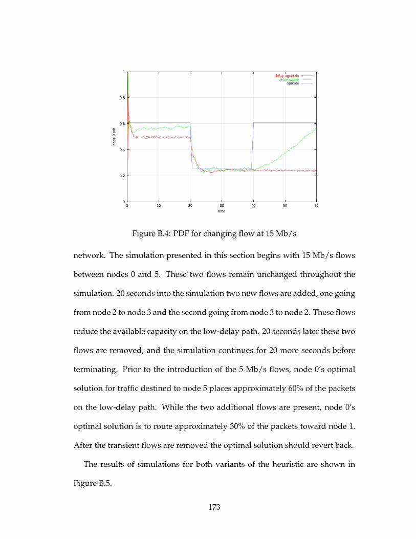
0
0.2
0.4
0.6
0.8
1
0 10 20 30 40 50 60
node
0 p
df
time
delay agnosticdelay aware
optimal
Figure B.4: PDF for changing flow at 15 Mb/s
network. The simulation presented in this section begins with 15 Mb/s flows
between nodes 0 and 5. These two flows remain unchanged throughout the
simulation. 20 seconds into the simulation two new flows are added, one going
from node 2 to node 3 and the second going from node 3 to node 2. These flows
reduce the available capacity on the low-delay path. 20 seconds later these two
flows are removed, and the simulation continues for 20 more seconds before
terminating. Prior to the introduction of the 5 Mb/s flows, node 0’s optimal
solution for traffic destined to node 5 places approximately 60% of the packets
on the low-delay path. While the two additional flows are present, node 0’s
optimal solution is to route approximately 30% of the packets toward node 1.
After the transient flows are removed the optimal solution should revert back.
The results of simulations for both variants of the heuristic are shown in
Figure B.5.
173

0
0.2
0.4
0.6
0.8
1
0 10 20 30 40 50 60
node
0 p
df
time
delay agnosticdelay aware
optimal
Figure B.5: PDF for changing flow at 15 Mb/s
As with the previous simulations, the simulated behavior matches the ex-
pected behavior. Both variations are close to optimal during the first 20 sec-
onds. Once the change is made both adapt to where only 20% of the packets
are being routed toward node 1. After the transient flows are removed the
delay-agnostic variation makes no effort to revert while the delay-aware varia-
tion begins to adapt slowly.
B.3 Summary
The heuristic was consistently able to adapt to changes in its environment. In
the case of the delay-agnostic heuristic, only changes resulting in loss caused
reconvergence. The delay-aware heuristic would continue to search for lower-
delay solutions. It had the desired attribute of rapidly responding to solutions
174

that would cause loss and slowly adapting to lower-delay solutions. This pro-
vides a measure of stability.
This work only considered simple topological changes, namely dropping or
adding a single edge. Node failure results in dropping many edges at the same
time. Evaluating the behavior of the heuristic in the presence of node failure is
left as future work.
175