symmetryS S

Article

A Genetic XK-Means Algorithm with EmptyCluster Reassignment

Chun Hua 1,2, Feng Li 1, Chao Zhang 1, Jie Yang 1 and Wei Wu 1,*1 School of Mathematical Sciences, Dalian University of Technology, Dalian 116024, China;

chunhua99018074@163.com (C.H.); dscling@126.com (F.L.); chao.zhang@dlut.edu.cn (C.Z.);yangjiee@dlut.edu.cn (J.Y.)

2 School of Computer Sciences and Technology, Inner Mongolia University for Nationalities,Tongliao 028043, China

* Correspondence: wuweiw@dlut.edu.cn

Received: 11 April 2019; Accepted: 24 May 2019; Published: 2 June 2019�����������������

Abstract: K-Means is a well known and widely used classical clustering algorithm. It is easy tofall into local optimum and it is sensitive to the initial choice of cluster centers. XK-Means(eXploratory K-Means) has been introduced in the literature by adding an exploratory disturbanceonto the vector of cluster centers, so as to jump out of the local optimum and reduce the sensitivityto the initial centers. However, empty clusters may appear during the iteration of XK-Means,causing damage to the efficiency of the algorithm. The aim of this paper is to introduce anempty-cluster-reassignment technique and use it to modify XK-Means, resulting in an EXK-Meansclustering algorithm. Furthermore, we combine the EXK-Means with genetic mechanism toform a genetic XK-Means algorithm with empty-cluster-reassignment, referred to as GEXK-Meansclustering algorithm. The convergence of GEXK-Means to the global optimum is theoreticallyproved. Numerical experiments on a few real world clustering problems are carried out, showing theadvantage of EXK-Means over XK-Means, and the advantage of GEXK-Means over EXK-Means,XK-Means, K-Means and GXK-Means (genetic XK-Means).

Keywords: K-Means; genetic mechanism; exploratory disturbance; global convergence; empty-cluster-reassignment

1. Introduction

Clustering algorithms are a class of unsupervised classification methods for a data set (cf. [1–5]).Roughly speaking, a clustering algorithm classifies the vectors in the data set such that distances ofthe vectors in the same cluster are as small as possible, and the distances of the vectors belonging todifferent clusters are as large as possible. Therefore, the vectors in the same cluster have the greatestsimilarity, while the vectors in different clusters have the greatest dissimilarity.

A clustering technique called K-Means is proposed and discussed in [1,2] among many others.Because of its simplicity and fast convergence speed, K-Means is widely used in various research fields.For instance, K-Means is used in [6] for removing the noisy data. A disadvantage of K-Means is that itis easy to fall into local optima. As a remedy, a popular trend is to integrate the genetic algorithm [7,8]with K-means to obtain genetic K-means algorithms [9–23]. K-Means is also combined with fuzzymechanism to obtain fuzzy C-Means [24,25].

A successful modification of K-Means is proposed in [26], referred to as XK-Means (eXploratoryK-Means). It adds an exploratory disturbance onto the vector of the cluster centers so as to jump out ofthe local optimum and to reduce the sensitivity to the initial centers. However, empty clusters mayappear during the iteration of XK-Means, which violates the condition that the number of clusters

Symmetry 2019, 11, 744; doi:10.3390/sym11060744 www.mdpi.com/journal/symmetry

Symmetry 2019, 11, 744 2 of 17

should be a pre-given number K and causes damage to the efficiency of the algorithm (see Remark 1 inSection 2.3 below for details). As a remedy, we propose in this paper to modify XK-Means in terms ofan empty-cluster-reassignment technique, resulting in an EXK-Means clustering algorithm.

The involvement of the exploratory disturbance in EXK-Means helps to jump out of the localoptimum during the iteration. However, in order to guarantee the convergence of the iteration process,the exploratory disturbance has to decrease and tend to zero in the iteration process. Therefore, it isstill possible for EXK-Means to fall into local optimum. To further resolve this problem, we followthe aforementioned strategy to combine the genetic mechanism with our EXK-Means, resulting in aclustering algorithm called GEXK-Means.

Numerical experiments on thirteen real world data sets are carried out, showing the higheraccuracies of our EXK-Means over XK-Means, and our GEXK-Means over GXK-Means, EXK-Means,XK-Means and K-Means: first, our GEXK-Means achieves the highest S, and the lowest MSE, DB and XB(see the next section for definitions of these evaluation tools) for all of the thirteen data sets. Therefore,GEXK-Means performs better than the other four algorithms. Second, the overall performance of ourEXK-Means is a little bit better than that of XK-Means, which shows the benefit of the introduction ofour empty cluster reassignment technique.

The numerical experiments also show that the execution times of EXK-Means are a little bit longerthan those of K-Means and XK-means, and the execution times of GEXK-Means are the longest in thefive algorithms. This is a disadvantage of EXK-Means and GEXK-Means. However, the computerspeed is getting high and high in nowadays, and sometimes the computational time does not mattervery much in practice if the data set is not very large. In case we do not mind a bit of an increase in thecomputational time and we care very much about the accuracy, our algorithm may be of value.

A probabilistic convergence of our GEXK-Means to the global optimum is theoretically proved.This paper is organized as follows. In Section 2, we describe the K-Means, XK-Means, GXK-Means,

and our proposed EXK-Means and GEXK-Means. In Section 3, numerical experiments are shownon GEXK-Means and its comparison with K-Means, XK-Means, GXK-Means and EXK-Means.The convergence of GEXK-Means to a globally optimal solution is theoretically proved in Section 4.Some short conclusions are drawn in Section 5.

2. Algorithms

In this section, we first give some notations and describe some evaluation tools. Then, we definethe clustering algorithms used in this paper.

2.1. Notations

Let us introduce some notations. Our task is to cluster a set of n genes {xi, i = 1, 2, ..., n} into Kclusters. Each gene is expressed as a vector of dimension D: xi = (xi1, xi2, · · · , xiD)

T . For i = 1, 2, ..., nand k = 1, 2, ..., K, we define

wik =

{1, if the i-th gene belongs to the k-th cluster,0, otherwise.

(1)

In addition, we define the label matrix W = [wik]. We require that each gene belongs to preciselyone cluster, and each cluster contains at least one gene. Therefore,

K

∑k=1

wik = 1, i = 1, 2, ..., n, (2)

1 ≤n

∑i=1

wik < n, k = 1, 2, ..., K. (3)

Symmetry 2019, 11, 744 3 of 17

Denote the center of the k-th cluster by ck = (ck1, ck2, . . . , ckD)T , defined as

ck =

n∑

i=1wikxi

n∑

i=1wik

. (4)

The Euclidean norm ||.|| will be used in our paper. Then, for any two D-dimensional vectorsy = (y1, y2, . . . , yD)

T and z = (z1, z2, . . . , zD)T in RD, the distance is

‖ y− z ‖= (D

∑i=1|yi − zi|2)

12 . (5)

2.2. Evaluation Strategies

In our numerical simulation, we will use the following evaluation tools: the mean squarederror (MSE), the Xie–Beni index (XB) [12], the Davies–Bouldin index (DB) [13,27], and the separationindex (S) [4]. The aim of the clustering algorithms discussed in this paper is to choose the optimalcenters ck’s and the optimal label matrix W so as to minimize the mean square error MSE. Then,MSE together with the indexes XB, DB and S will be applied to evaluate the outcome of theclustering algorithms.

MSE is defined by

MSE =1n

K

∑k=1

n

∑i=1

wik ‖ xi − ck ‖2 . (6)

MSE will be used as the evaluation function in the genetic operation of the numerical simulationlater on. Generally speaking, lower MSE means better clustering result.

The XB index [12] is defined as follows:

XB =MSEdmin

, (7)

where dmin is the shortest distance between cluster centers. Higher dmin means better clusteringresult. As we mentioned above, the MSE is the lower the better. Therefore, lower XB implies betterclustering results.

To define the DB index [13,27], we first defined the within-cluster separation Sk as

Sk = (1| Ck | ∑

xi∈Ck

‖ xi − ck ‖2)12 , (8)

where Ck (resp. |Ck|) denotes the set (resp. the number) of the samples belonging to the cluster k.Next, we define a term Rk for cluster ck as

Rk = maxj,j 6=k

Sk + Sj

‖ ck − cj ‖. (9)

Then, the DB index is defined as

DB =1K

K

∑k=1

Rk. (10)

Generally speaking, lower DB implies better clustering results.

Symmetry 2019, 11, 744 4 of 17

The separation index S [4] is defined as follows:

S =1

∑Kk,j=1;k 6=j |Ck||Cj|

K

∑k,j=1;k 6=j

|Ck||Cj| ‖ ck − cj ‖ . (11)

Generally speaking, higher S implies better clustering results.The Nemenyi test [28–30] will be used for evaluating the significance of differences of XK-Means

vs. EXK-Means and GXK-Means vs. GEXK-Means, respectively. The function cdf.chisq of SPSSsoftware (SPSS Statistics 17.0, IBM, New York, USA) is used to compute the significance probabilityPr. The value of Pr is in between 0 and 1. The smaller value of Pr implies the bigger significance ofthe difference of the two groups. One can say that the difference of the two groups is significant if Pris less than a particular threshold value. The most often used threshold values are 0.01, 0.05 and 0.1.The threshold value 0.05 will be adopted in this paper.

The relative error ReError defined below will be used for a stop criterion in our numericaliteration process:

ReError = |MSEt−1 −MSEt

MSEt|, (12)

where MSEt and MSEt−1 denote the values of MSE in the current and previous iteration steps, respectively.

2.3. XK-Means

Trying to jump out of the local minimum, the XK-Means algorithm is proposed in [26], where theusual K-Means is modified by adding an exploratory vector onto each cluster center as follows:

c∗k = ck + θk, (13)

where θk is a D-dimensional exploratory vector at the current step. It is used to disturb the centerproduced by K-Means operation, and its component is randomly chosen as

(θk)i = rand(ai, bi) ∗ randsign(i), i = 1, 2, . . . , D, (14)

where bi is a given positive number, andai = βbi, (15)

with a given factor β ∈ [0, 1). In general, the disturbance should be decreased with the increase of theiteration step. Thus, for a new iteration step, the new value of bi is set to be

b∗i = αbi, (16)

with a given factor α ∈ [0, 1).

Remark 1. Empty cluster will not appear in a usual K-Means iteration process. However, it is possible forXK-Means to produce an empty cluster in the iteration process. This happens when the exploratory vector θk inFormula (13) drives the center ck away from the genes in the k-th cluster, such that all these genes join anothercluster in the re-organization stage of the XK-Means and leave the k-th cluster empty. Then, the XK-Meansiteration will end up with the number of clusters less than K, which violates the condition that the number ofclusters should be K.

2.4. EXK-Means

Due to the disturbance θk, the XK-Means algorithm may produce empty clusters during theiteration process, which violates condition (3). The reason for such a cluster to become empty is that itis too close to, and is attracted into other cluster when the centers are disturbed by the θk’s. In this

Symmetry 2019, 11, 744 5 of 17

sense, it seems reasonable for such a cluster to “disappear”. However, on the other hand, the emptyclusters will damage the clustering efficiency due to the decrease of the number of working clusters.

To resolve this problem, our idea is to re-assign such an empty cluster by a vector that isfarthest to its center. Specifically, our EXK-Means modifies the XK-means by applying the followingEmpty-cluster-reassignment procedure when empty clusters appear after an XK-Means iteration step.

Empty-cluster-reassignment procedure:

1. Let K0 be the number of empty clusters, 1 ≤ K0 < K.2. Find the most marginal point of each non-empty cluster: x∗k = arg maxxi∈Ck ‖ xi − ck ‖, where Ck

is the set of genes in the k-th cluster.3. Sort {x∗1 , x∗2 , ..., x∗K} in descending order according to their distances to the corresponding centroids

to get {x∗∗1 , x∗∗2 , ..., x∗∗K }.4. Take the first K0 genes from {x∗∗1 , x∗∗2 , ..., x∗∗K } to form K0 new centers {x∗∗1 }, {x∗∗2 }, ..., {x∗∗K0

}.5. Adjust the partition of genes according to original centers and the new K0 centers.

2.5. Genetic Operations

As we argued in the Introduction, although EXK-Means and XK-Means algorithms improvethe K-Means on the local minimum issue, but the possibility remains for them to fall into localoptimum. We try to combine a genetic mechanism with the EXK-Means to get the global convergence.In particular, we propose to use the following genetic operations:

2.5.1. Label Vectors

For the convenience of genetic operation, in place of the label matrix W, let us introduce then-dimensional label vector

L = (l1, l2, . . . , li, . . . , ln)T , (17)

where each component li ∈ {1, 2, . . . , K} represents the cluster label of xi, as in [10]. Let N denote thepopulation size. Then, we write the population set as {Lj, j = 1, 2, . . . , N}.

2.5.2. Initialization

To avoid empty clusters in the initialization stage, we initialize the population as follows.First, the top K components of each Lj are randomly assigned as a permutation of {1, 2, . . . , K}.Secondly, the other components of Lj are assigned as random cluster numbers respectively selectedfrom the uniform distribution of the {1, 2, . . . , K}.

2.5.3. Selection

The usual roulette strategy is used for the random selection. The probability that an individual Lj

is selected from the existing population to breed the next generation is given by

P(Lj) =F(Lj)

N∑

h=1F(Lh)

, j = 1, 2, . . . , N, (18)

F(Lj) =1

1n

K∑

k=1

n∑

i=1wik||xi − ck||

, (19)

where F(Lj) is the reciprocal of MSE and represents the fitness value of the individual Lj in the population.

Symmetry 2019, 11, 744 6 of 17

2.5.4. Mutation

The mutation probability is denoted by Pm, which determines whether an individual Lj will bemutated. If an individual Lj is to be mutated, the translation probability of its component li to be k isdefined as

Pik = P{li = k} = 2dimax − ||xi − ck||

K∑

l=1(2di

max − ||xi − cl ||), (20)

dimax = max

k{||xi − ck||}, (21)

where i = 1, 2, . . . , n, k = 1, 2, . . . , K. To avoid empty individuals after mutation operation, li ismutated only when the li-th cluster contains more than two genes.

2.5.5. Three Steps EXK-Means

A three-step EXK-Means is applied for rapid convergence. For an individual L, it is updatedthrough the following operations: calculate the cluster centers by using (4) for the given L;add the exploratory vector and update the cluster centers by using (13); reassign each gene to thecluster with the closest cluster center to form a new individual L; correct the new L by using theEmpty-cluster-reassignment procedure in Section 2.4 if it contains empty cluster(s) at this moment.Repeat the process three times, and finally form an individual L of the next generation.

2.6. Genetic XK-Means ( GXK-Means )

The GXK-Means is briefly described as follows:

1. Initialization: Set the population size N, the maximum number of iterations T, the mutationprobability Pm, the number of clusters K and the error tolerance ETol . Let t = 0, and choose theinitial population P(0) according to Section 2.5.2. In addition, choose the best individual fromP(0) and denote it as super individual L∗(0).

2. Selection: Select a new population from P(t) according to Section 2.5.3, and denote it by P1(t).3. Mutation: Mutate each individual in P1(t) according to Section 2.5.4, and get a new population

denoted by P2(t).4. XK-Means: Perform XK-Means on P2(t) three times to get the next generation population denoted

by P(t + 1).5. Update the super individual: choose the best individual from P(t + 1) and compare it with L∗(t)

to get L∗(t + 1).6. Stop if either t = T or ReError ≤ ETol (see (12)), otherwise go to 2 with t← t + 1.

2.7. GEXK-Means (Genetic EXK-Means)

The process of GEXK-Means proposed in this paper is as follows:

1. Initialization: Set the population size N, the maximum number of iterations T, the mutationprobability Pm, the number of clusters K and the error tolerance ETol . Let t = 0, and choose theinitial population P(0) according to Section 2.5.2. In addition, choose the best individual fromP(0) and denote it as super individual L∗(0).

2. Selection: Select a new population from P(t) according to Section 2.5.3, and denote it by P1(t).3. Mutation: Mutate each individual in P1(t) according to Section 2.5.4, and get a new population

denoted by P2(t).4. EXK-Means: Perform the three steps EXK-Means on P2(t) according to Section 2.5.5 to get the

next generation population denoted by P(t + 1).5. Update the super individual: choose the best individual from P(t + 1) and compare it with L∗(t)

to get L∗(t + 1).6. Stop if either t = T or ReError ≤ ETol (see (12)), otherwise go to 2 with t← t + 1.

Symmetry 2019, 11, 744 7 of 17

Let us explain the functions of the four operations in the GEXK-Means: selection, mutation,EXK-Means and updating of the super individual. The selection operation encourages the populationto have a good evolution direction. The function of the EXK-Means operation is local search for betterindividuals. The mutation operation guarantees the ergodicity of the evolution process, which in turnguarantees the appearance of a global optimal individual in the evolution process. Finally, the updatingoperation of the super individual will catch forever the global optimal individual once it appears.

3. Experimental Evaluation and Results

3.1. Data Sets and Parameters

Thirteen data sets shown in Table 1 are used for evaluating our algorithms. The first five datasets are gene expression data sets, including Sporulation [31], Yeast Cell Cycle [32], Lymphoma [33],and two UCI data sets Yeast and Ecoli. The other eight are UCI data sets, which are not gene expressdata sets.

As shown in Table 1, Sporulation, Yeast Cell Cycle and Lymphoma data sets contain some samplevectors with missing component values. To rectify these defective data, we follow the strategy adoptedin [34–36]: the sample vectors with more than 20% missing components are removed from the data sets.In addition, for the sample vectors with less than 20% missing components, the missing componentvalues are estimated by the KNN algorithm with the parameter k = 15 as in [35], where k is the numberof the neighboring vectors used to estimate the missing component value (see [34–36] for details).Here, we point out that this parameter k here is different from the index k we have used in this paperfor denoting the k-th cluster.

Table 1. Data sets used in experiments.

Data SetsNo. of No. of Vectors No. of Vectors No. of No. ofVectors with Missing with Missing Attributes Classes

n Components <20% Component ≥20% D K

Sporulation 6023 413 198 7 16Yeast Cell Cycle 6078 5498 680 77 256

Lymphoma 4022 3166 3 96 150Yeast 1484 0 0 8 10Ecoli 336 0 0 8 7

Dermatology 366 8 0 34 6Glass Identification 214 0 0 10 7

Image Segmentation 2310 0 0 20 7Wine Quality 4898 0 0 12 7

Wireless Indoor Localization 2000 0 0 7 4Statlog Vehicle 946 0 0 18 4

Page Blocks Classification 5473 0 0 10 6Wine 178 0 0 13 3

The values of the parameters used in the computation are set as follows:

Population size n = 20 (cf. Sections 2.6 and 2.7)Mutation probability Pm = 0.1 (cf. Sections 2.6 and 2.7)Error tolerance ETol = 0.001 (cf. Sections 2.2, 2.6 and 2.7)α = 0.3 (cf. (14), (16))β = 0.95 (cf. (14), (15))T = 150 (cf. Sections 2.6 and 2.7)

In the experiments, we use two different computers: M1 (Intel (R), Core (TM) i3-8100 CPU and 4 GBRAM, Santa Clara, CA, USA) and M2 (Intel (R), Core (TM) i5-7400 CPU and 8 GB RAM). The softwareMatlab (Matlab 2017b, Math Works, Natick, MA, USA) is used to implement the clustering algorithms.

Symmetry 2019, 11, 744 8 of 17

3.2. Experimental Results and Discussion

We divide this subsection into three parts. The first part concerns with the performances of thealgorithms in terms of MSE, S, DB and XB. The second part demonstrates the significance of differencesof the algorithms in terms of Nemenyi Test. The third part presents the computational times of thealgorithms. We shall pay our attention mainly on the comparisons of EXK-Means vs. XK-Meansand GEXK-Means vs. GXK-Means, respectively, so as to show the benefit of the introduction of ourempty-cluster-reassignment technique.

3.2.1. MSE, S, DB and XB Performances

Each of the five algorithms conducted fifty trials on the thirteen data sets. The averages over thefifty trials for the four evaluation criteria (MSE, S, DB and XB) are listed in Tables 2 and 3, devoted tothe five gene expression data sets and the other eight UCI data sets, respectively.

Table 2. Average MSE, S, DB and XB on the gene data sets.

Data Sets AlgorithmMSE S DB XB

(Lower the (Higher the (Lower the (Lower the Better)Better) Better) Better)

Yeast Cell Cycle

K-Means 2.3092 3.1637 2.6990 5.0987× 10−4

XK-Means 2.2753 3.1773 2.5595 4.9905× 10−4

EXK-Means 2.2728 3.2170 2.0686 4.7811× 10−4

GXK-Means 2.2623 3.2560 2.4612 3.8156× 10−4

GEXK-Means 2.2572 3.2625 1.8070 3.6357× 10−4

Sporulation

K-Means 0.8959 2.7612 1.5781 3.0905× 10−4

XK-Means 0.8968 2.7556 1.5261 3.0761× 10−4

EXK-Means 0.8987 2.7315 1.6226 2.8585× 10−4

GXK-Means 0.8961 2.7510 1.5207 1.7465× 10−4

GEXK-Means 0.8951 2.7674 1.3285 1.5321× 10−4

Lymphoma

K-Means 4.8762 7.1725 2.8532 7.4561× 10−4

XK-Means 4.7683 7.2998 2.7294 7.1749× 10−4

EXK-Means 4.7764 7.2890 2.5627 5.7017× 10−4

GXK-Means 4.7520 7.3296 2.3285 5.7929× 10−4

GEXK-Means 4.7244 7.3787 2.1489 5.0597× 10−4

Yeast

K-Means 0.1613 0.3106 1.6854 9.6311× 10−4

XK-Means 0.1586 0.3192 1.3592 8.6864× 10−4

EXK-Means 0.1607 0.3234 1.3701 9.0603× 10−4

GXK-Means 0.1581 0.3194 1.2621 6.3508× 10−4

GEXK-Means 0.1560 0.3296 0.9154 4.2514× 10−4

Ecoli

K-Means 0.2914 3.3151 1.4452 7.6× 10−3

XK-Means 0.2880 3.2775 1.0973 5.9× 10−3

EXK-Means 0.2382 3.7191 0.7127 3.3× 10-3

GXK-Means 0.2321 3.4022 0.3364 3.1× 10−3

GEXK-Means 0.2268 3.7791 0.3021 1.1× 10−3

Symmetry 2019, 11, 744 9 of 17

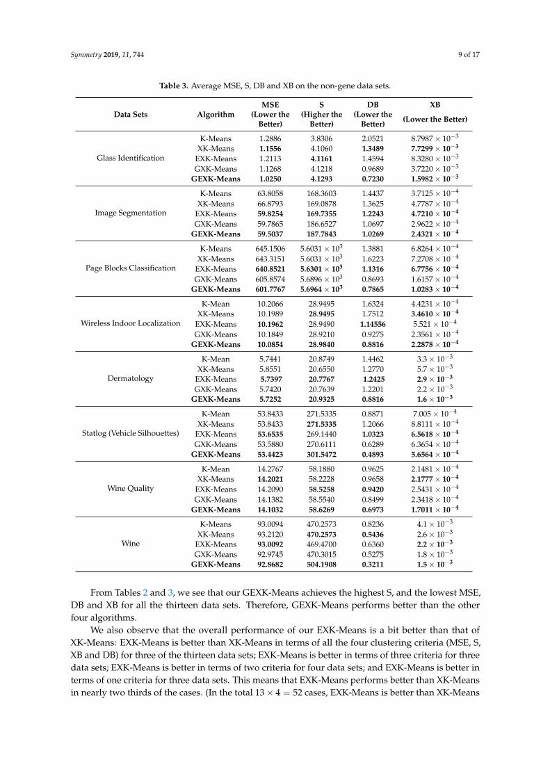
Table 3. Average MSE, S, DB and XB on the non-gene data sets.

Data Sets AlgorithmMSE S DB XB

(Lower the (Higher the (Lower the (Lower the Better)Better) Better) Better)

Glass Identification

K-Means 1.2886 3.8306 2.0521 8.7987× 10−3

XK-Means 1.1556 4.1060 1.3489 7.7299× 10−3

EXK-Means 1.2113 4.1161 1.4594 8.3280× 10−3

GXK-Means 1.1268 4.1218 0.9689 3.7220× 10−3

GEXK-Means 1.0250 4.1293 0.7230 1.5982× 10−3

Image Segmentation

K-Means 63.8058 168.3603 1.4437 3.7125× 10−4

XK-Means 66.8793 169.0878 1.3625 4.7787× 10−4

EXK-Means 59.8254 169.7355 1.2243 4.7210× 10−4

GXK-Means 59.7865 186.6527 1.0697 2.9622× 10−4

GEXK-Means 59.5037 187.7843 1.0269 2.4321× 10−4

Page Blocks Classification

K-Means 645.1506 5.6031× 103 1.3881 6.8264× 10−4

XK-Means 643.3151 5.6031× 103 1.6223 7.2708× 10−4

EXK-Means 640.8521 5.6301× 103 1.1316 6.7756× 10−4

GXK-Means 605.8574 5.6896× 103 0.8693 1.6157× 10−4

GEXK-Means 601.7767 5.6964× 103 0.7865 1.0283× 10−4

Wireless Indoor Localization

K-Mean 10.2066 28.9495 1.6324 4.4231× 10−4

XK-Means 10.1989 28.9495 1.7512 3.4610× 10−4

EXK-Means 10.1962 28.9490 1.14556 5.521× 10−4

GXK-Means 10.1849 28.9210 0.9275 2.3561× 10−4

GEXK-Means 10.0854 28.9840 0.8816 2.2878× 10−4

Dermatology

K-Mean 5.7441 20.8749 1.4462 3.3× 10−3

XK-Means 5.8551 20.6550 1.2770 5.7× 10−3

EXK-Means 5.7397 20.7767 1.2425 2.9× 10−3

GXK-Means 5.7420 20.7639 1.2201 2.2× 10−3

GEXK-Means 5.7252 20.9325 0.8816 1.6× 10−3

Statlog (Vehicle Silhouettes)

K-Mean 53.8433 271.5335 0.8871 7.005× 10−4

XK-Means 53.8433 271.5335 1.2066 8.8111× 10−4

EXK-Means 53.6535 269.1440 1.0323 6.5618× 10−4

GXK-Means 53.5880 270.6111 0.6289 6.3654× 10−4

GEXK-Means 53.4423 301.5472 0.4893 5.6564× 10−4

Wine Quality

K-Mean 14.2767 58.1880 0.9625 2.1481× 10−4

XK-Means 14.2021 58.2228 0.9658 2.1777× 10−4

EXK-Means 14.2090 58.5258 0.9420 2.5431× 10−4

GXK-Means 14.1382 58.5540 0.8499 2.3418× 10−4

GEXK-Means 14.1032 58.6269 0.6973 1.7011× 10−4

Wine

K-Means 93.0094 470.2573 0.8236 4.1× 10−3

XK-Means 93.2120 470.2573 0.5436 2.6× 10−3

EXK-Means 93.0092 469.4700 0.6360 2.2× 10−3

GXK-Means 92.9745 470.3015 0.5275 1.8× 10−3

GEXK-Means 92.8682 504.1908 0.3211 1.5× 10−3

From Tables 2 and 3, we see that our GEXK-Means achieves the highest S, and the lowest MSE,DB and XB for all the thirteen data sets. Therefore, GEXK-Means performs better than the otherfour algorithms.

We also observe that the overall performance of our EXK-Means is a bit better than that ofXK-Means: EXK-Means is better than XK-Means in terms of all the four clustering criteria (MSE, S,XB and DB) for three of the thirteen data sets; EXK-Means is better in terms of three criteria for threedata sets; EXK-Means is better in terms of two criteria for four data sets; and EXK-Means is better interms of one criteria for three data sets. This means that EXK-Means performs better than XK-Meansin nearly two thirds of the cases. (In the total 13× 4 = 52 cases, EXK-Means is better than XK-Means

Symmetry 2019, 11, 744 10 of 17

for 3× 4 + 3× 3 + 2× 4 + 1× 3 = 32 cases.) The better case is marked by black face number inTables 2 and 3.

To see more clearly the overall performance, in Figures 1–4 for MSE, DB, XB and S evaluationsrespectively, we further present the average performances of the five algorithms over the thirteen datasets. These figures clearly show that, in the sense of average performance, the proposed GEXK-Meansoutperforms the other four algorithms, and EXK-Means outperforms K-Means and XK-Means.

Figure 1. Average MSE of thirteen data sets (The value of MSE is the lower the better).

Figure 2. Average DB of thirteen data sets (The value of DB is the lower the better).

Figure 3. Average XB of thirteen data sets (The value of XB is the lower the better).

Symmetry 2019, 11, 744 11 of 17

Figure 4. Average S of thirteen data sets (The value of S is the higher the better).

As an example to show what happens in the iteration processes, a typical iteration process onYeast Cell Cycle data set is shown in Figures 5–8, presenting the MSE, XB, DB and S curves respectivelyfor the five algorithms.

Figure 5. MSE curves of the algorithms for Yeast Cell Cycle (The value of MSE is the lower the better).

Symmetry 2019, 11, 744 12 of 17

Figure 6. DB curves of the algorithms for Yeast Cell Cycle (The value of DB is the lower the better).

Figure 7. XB curves of the algorithms for Yeast Cell Cycle (The value of XB is the lower the better).

Figure 8. S curves of the algorithms for Yeast Cell Cycle (The value of S is the higher the better).

Symmetry 2019, 11, 744 13 of 17

3.2.2. Nemenyi Test

Table 4 shows the results of Nemenyi Test on MSE, S, DB and XB indexes. We use the thresholdvalue 0.05 for the significance evaluation. For DB index, EXK-Means shows significant differencecompared with XK-Means, while EXK-Means does not show significant difference compared withXK-Means for the other three indexes. For all four of the indexes, GEXK-Means shows a significantdifference compared with GXK-Means.

Table 4. Nemenyi Test for multiple comparisons.

Groups for Comparison Evaluation Technique Pr

XK-Means vs. EXK-Means

MSE 0.8994S 0.6691

DB 0.0421XB 0.4539

GXK-Means vs. GEXK-Means

MSE 0.0492S 0.0412

DB 0.0409XB 0.0403

3.2.3. Computational Time

Table 5 gives the average computational times over the fifty runs for each data set. It shows that thecomputational times of EXK-Means are a little bit longer than those of K-Means and XK-means, and thecomputational times of GEXK-Means are a little bit longer than those of GXK-Means. This indicatesthat the introduction of our empty-cluster-reassignment technique increases the computational time.However, our algorithms are better if we do not mind a bit of increase in the computational time andwe care very much about the accuracy.

Table 5. Average running times (in seconds).

Data Sets Evaluation K XK EXK GXK GEXK MachineTechnique -Means -Means -Means -Means -Means

Sporulation

MSE 11.368 11.689 12.56 289.656 688.552 M2S 11.464 11.792 12.61 256.782 689.457 M2

DB 10.424 10.569 10.480 239.529 662.183 M2XB 9.632 9.881 9.878 269.364 396.33 M2

MSE 58.65 60.213 64.52 4867.560 5432.23 M2Yeast S 58.87 60.351 65.11 4789.108 5433.69 M2

Cell Cycle DB 69.425 72.37 73.06 4965.682 5654.75 M2XB 52.584 56.321 59.66 4754.538 5014.56 M2

Lymphoma

MSE 69.425 70.43 74.332 4962.224 5321.6 M2S 69.661 71.34 74.994 4987.300 5324.1 M2

DB 72.135 77.483 74.286 4753.626 5332.42 M2XB 62.526 66.36 68.665 4665.186 5026.559 M2

MSE 0.3675 0.368 0.2975 19.566 20.824 M1Glass S 0.3678 0.371 0.2980 19.960 20.885 M1

Identification DB 0.505 0.535 0.536 19.325 27.687 M1XB 0.267 0.303 0.304 16.263 19.806 M1

MSE 4.552 4.230 4.336 298.128 361.755 M1Image S 4.578 4.257 4.402 296.867 363.455 M1

Segmentation DB 4.564 4.663 4.718 286.692 382.924 M1XB 4.565 4.131 4.183 263.960 332.092 M1

Symmetry 2019, 11, 744 14 of 17

Table 5. Cont.

Data Sets Evaluation K XK EXK GXK GEXK MachineTechnique -Means -Means -Means -Means -Means

MSE 4.039 4.078 4.122 382.663 395.273 M1Page Blocks S 4.165 4.216 4.269 378.632 397.421 M1

Classification DB 7.859 7.649 7.947 376.657 520.118 M1XB 4.596 4.622 4.264 296.186 390.57 M1

Yeast

MSE 1.810 1.964 1.870 159.200 165.08 M1S 1.914 1.998 1.978 161.230 167.1 M1

DB 3.630 3.784 3.800 163.620 241.346 M1XB 1.718 1.817 1.847 148.960 161.346 M1

MSE 1.428 1.430 1.433 119.630 122.278 M1Wireless Indoor S 1.473 1.459 1.62 120.775 124.512 M1

Localization DB 2.843 2.760 2.840 124.360 176.689 M1XB 1.436 1.445 1.418 98.641 120.628 M1

Ecoli

MSE 0.408 0.437 0.437 29.611 30.494 M1S 0.409 0.441 0.439 29.845 30.569 M1

DB 0.736 0.858 0.882 28.010 43.321 M1XB 0.399 0.447 0.490 29.380 31.22 M1

Dermatology

MSE 0.634 0.635 0.710 23.450 24.829 M1S 0.639 0.651 0.786 24.687 25.854 M1

DB 0.78 0.832 0.857 24.312 26.758 M1XB 0.406 0.542 0.516 23.720 26.811 M1

MSE 0.705 0.726 0.768 53.856 57.061 M1Statlog S 0.712 0.732 0.798 55.289 58.067 M1

(Vehicle Silhouettes) DB 1.298 1.303 1.351 58.450 77.966 M1XB 0.590 0.634 0.642 43.892 51.137 M1

Wine Quality

MSE 4.538 4.658 4.758 386.680 444.963 M1S 4.563 4.713 4.799 379.668 446.921 M1

DB 8.435 8.512 8.571 412.654 565.498 M1XB 4.463 4.499 4.635 356.215 421.432 M1

Wine

MSE 0.159 0.182 0.179 10.226 11.133 M1S 0.161 0.188 0.182 10.129 11.186 M1

DB 0.267 0.304 0.309 11.636 13.852 M1XB 0.152 0.172 0.174 8.385 10.130 M1

4. Convergence

In this section, the convergence properties of GEXK-Means are analyzed. It is clear that thereexist m = Kn possible solutions when classifying n genes into K clusters. As mentioned in Section 2.5,every possible solution can be denoted as a label vector L. Therefore, the number of all possibleindividuals is m. Let L ∗ be the set of global optimal individuals with maximum fitness value.

For an individual L that will to be mutated, according to Eqution (20), we have

Pik = P{li = k} = 2dimax − ||xi − ck||

K∑

l=1(2di

max − ||xi − cl ||),

where i = 1, 2, . . . , n, k = 1, 2, . . . , K, and dimax > ||xi − ck|| > 0. Therefore, 2di

max − ||xi − ck|| > 0,and Pik > 0, i = 1, 2, . . . , n, k = 1, 2, . . . , K. We note that the number of genes and the numberof clusters are finite. Therefore, Pik (i = 1, 2, . . . , n, k = 1, 2, . . . , K) has lower bound denoted byM > 0. This means that every gene can be mutated into any one cluster with positive probability.In particular, L can be mutated into any other individuals with positive probability. Recall that

Symmetry 2019, 11, 744 15 of 17

P(t) = {L1(t), L2(t), . . . , LN(t)} is the population at step t. Let PLj(t)→L ∗ stand for the probability in

which Lj(t) is mutated to one of the global optimal individuals. Then

PLj(t)→L ∗ > Mn, j = 1, 2, . . . , N. (22)

Let PMutation stand for the probability generating the optimal individual in P2(t) by mutationoperation. Then,

PMutation =N

∑j=1

PmP(Lj(t))(PLj(t)→L ∗)

> Pm

N

∑j=1

P(Lj(t))Mn

= Pm Mn

> 0,

(23)

where Pm > 0 is the mutation probability, P(Lj(t)) > 0 is the selection probability defined by Equation(18), and ∑N

j=1 P(Lj(t)) = 1.

Theorem 1. When the GEXK-Means defined in Section 2.7 is applied for the classification of a given data set,the global optimal classification result for the data set will appear and will be caught with probability 1 in aninfinite evolution iteration process of the GEXK-Means.

Proof. Along with the evolution process, the updating operation of the super individual will keep thesuper individual denoted by L∗(t) of every generation t = 0, 1, 2, . . .. According to (22), we know thatthe L∗(t) may become a global optimal individual with positive probability. According to the SmallProbability Event Principle [37,38], the global optimum individual will appear in the super individualsequence with probability 1 when the evolution iteration process goes to infinity. This proves theglobal convergence of GEXK-Means.

We remark that the global convergence stated above is of a theoretical and probabilistic nature.It does not guarantee that the convergence to a global optimum can be reached in finite number ofGEXK-Means iterations.

5. Conclusions

XK-Means (eXploratory K-Means) is a popular data clustering algorithm. However, emptyclusters may appear during the iteration of XK-Means, which violates the condition that the numberof clusters should be K and causes damage to the efficiency of the algorithm. As a remedy,we define an empty-cluster-reassignment technique to modify XK-Means when empty clusters appear,resulting in an EXK-Means clustering algorithm. Furthermore, we combine the EXK-Means withgenetic mechanism to form a GEXK-Means clustering algorithm.

Numerical simulations are carried out on the comparison of K-Means, XK-Means, EXK-Meansand GXK-Means (genetic XK-Means) and GEXK-Means. The evaluation tools include the meansquared error (MSE), the Xie–Beni index (XB), the Davies–Bouldin index (DB) and the separationindex (S). The Nemenyi Test for multiple comparisons is also done on MSE, S, DB and XB, respectively.Thirteen real world data sets are used for the simulation. The running times of these algorithms arealso considered.

The conclusions we draw from the simulation results are as follows: first, the overall performancesof EXK-Means in terms of the four indexes outperform those of XK-Means, and the overallperformances of GEXK-Means outperform those of GXK-Means. This shows the effectiveness ofthe introduction of the empty-cluster-reassignment technique. Secondly, if we take the threshold

Symmetry 2019, 11, 744 16 of 17

value as 0.05 for the Nemenyi Test, then GEXK-Means shows a significant difference compared withGXK-Means for all four of the indexes. However, EXK-Means shows a significant difference comparedwith XK-Means only for the DB index. Thirdly, our EXK-Means and GEXK-Means take a little bit morecomputational time than XK-Means and GXK-Means, respectively.

The following global convergence of the GEXK-Means is also theoretically proved: the globaloptimum will appear and will be caught in the evolution process of GEXK-Means with probability 1.

Author Contributions: C.H. developed the mathematical model, carried out the numerical simulations and wrotethe manuscript; W.W. advised on developing the learning algorithms and supervised the work; F.L. contributed tothe theoretical analysis; C.Z. and J.Y. helped in the numerical simulations.

Funding: This research was supported by the National Science Foundation of China (No: 61473059), and theFundamental Research Funds for the Central Universities of China.

Conflicts of Interest: The authors declare that there are no conflicts of interest regarding the publication ofthis paper.

References

1. Steinhaus, H. Sur la division des corp materiels en parties. Bull. Acad. Polon. Sci. 1956, 3, 801–804.2. Macqueen, J. Some Methods for Classification and Analysis of MultiVariate Observations. In Proceedings of

the 5th Berkeley Symposium on Mathematical Statistics and Probability, Los Angeles, CA, USA, 21 June–18July 1967.

3. Wlodarczyk-Sielicka, M. Importance of Neighborhood Parameters During Clustering of Bathymetric DataUsing Neural Network. In Proceedings of the 22nd International Conference, Duruskininkai, Lithuania,13–15 October 2016.

4. Du, Z.; Wang, Y. PK-Means: A New Algorithm for Gene Clustering. Comput. Biol. Chem. 2008, 32, 243–247.[CrossRef] [PubMed]

5. Lin, F.; Du, Z. A Novel Parallelization Approach for Hierarchical Clustering. Parallel Comput. 2005,31, 523–527.

6. Santhanam, T.; Padmavathi, M.S. Application of K-Means and Genetic Algorithms for Dimension Reductionby Integrating SVM for Diabetes Diagnosis. Procedia Comput. Sci. 2015, 47, 76–83. [CrossRef]

7. Deep, K.; Thakur, M. A New Mutation Operator for Real Coded Genetic Algorithms. Appl. Math. Comput.2007, 193, 211–230. [CrossRef]

8. Ming, L.; Wang, Y. On Convergence Rate of a Class of Genetic Algorithms. In Proceedings of the WorldAutomation Congress, Budapest, Hungary, 24–26 July 2006.

9. Maulik, U. Genetic Algorithm Based Clustering Technique. Pattern Recognit. 2000, 33, 1455–1465. [CrossRef]10. Jones, D.R.; Beltramo, M.A. Solving Partitioning Problems with Genetic Algorithms. In Proceedings of the

4th International Conference on Genetic Algorithms, San Diego, CA, USA, 13–16 July 1991.11. Zheng, Y.; Jia, L.; Cao, H. Multi-Objective Gene Expression Programming for Clustering. Inf. Technol. Control

2012, 41, 283–294. [CrossRef]12. Xie, X.L.; Beni, G. A Validity Measure for Fuzzy Clustering. IEEE Trans. Pattern Anal. Mach. Intell. 1991,

13, 841–847. [CrossRef]13. Liu, Y.G. Automatic Clustering Using Genetic Algorithms. Appl. Math. Comput. 2011, 218, 1267–1279.

[CrossRef]14. Krishna, K.; Murty, M.N. Genetic K-Means Algorithm. IEEE Trans. Syst. Man Cybern. 1999, 29, 433–439.

[CrossRef]15. Bouhmala, N.; Viken, A. Enhanced Genetic Algorithm with K-Means for the Clustering Problem. Int. J.

Model. Optim. 2015, 5, 150–154. [CrossRef]16. Sheng, W.G.; Tucker, A. Clustering with Niching Genetic K-means algorithm. In Proceedings of the

6th Annual Genetic and Evolutionary Computation Conference (GECCO 2004), Seattle, WA, USA,26–30 June 2004.

17. Zhou, X.B.; Gu, J.G. An Automatic K-Means Clustering Algorithm of GPS Data Combining a Novel NicheGenetic Algorithm with Noise and Density. ISPRS Int. J. Geo-Inf. 2017, 6, 392–397. [CrossRef]

Symmetry 2019, 11, 744 17 of 17

18. Islam, M.Z.; Estivill-Castro, V.; Rahman, M.A.; Bossomaier, T. Combining K-Means and a Genetic Algorithmthrough a Novel Arrangement of Genetic Operators for High Quality Clustering. Expert Syst. Appl. 2018,91, 402–417. [CrossRef]

19. Michael, L.; Sumitra, M. A Genetic Algorithm that Exchanges Neighboring Centers for k-means clustering.Pattern Recognit. Lett. 2007, 28, 2359–2366.

20. Ishibuchi, H.; Yamamoto, T. Fuzzy Rule Selection by Multi-objective Genetic Local Search Algorithms andRule Evaluation Measures in Data Mining. Fuzzy Sets Syst. 2004, 141, 59–88. [CrossRef]

21. Zubova, J.; Kurasova, O. Dimensionality Reduction Methods: The Comparison of Speed and Accuracy.Inf. Technol. Control 2018, 47, 151–160. [CrossRef]

22. Wozniak, M.; Polap, D. Object Detection and Recognition via Clustered Features. Neurocomputing 2018,320, 76–84. [CrossRef]

23. Anusha, M.; Sathiaseelan, G.R. Feature Selection Using K-Means Genetic Algorithm for Multi-objectiveOptimization. Procedia Comput. Sci. 2015, 57, 1074–1080. [CrossRef]

24. Bezdek, J.C.; Ehrlich, R. FCM: The Fuzzy C-Means Clustering Algorithm. Comput. Geosci. 1984, 10, 191–203.[CrossRef]

25. Indrajit, S.; Ujjwal, M. A New Multi-objective Technique for Differential Fuzzy Clustering. Appl. Soft Comput.2011, 11, 2765–2776.

26. Lam, Y.K.; Tsang, P.W.M. eXplotatory K-Means: A New Simple and Efficient Algorithm for Gene Clustering.Appl. Soft. Comput. 2012, 12, 1149–1157. [CrossRef]

27. Davies, D.L.; Bouldin, D.W. A Cluster Separation Measure. IEEE Trans. Pattern Anal. Mach. Intell. 1979,PAMI-1, 224–227. [CrossRef]

28. Liu, Y.W.; Chen, W.H. A SAS Macro for Testing Differences among Three or More Independent Groups UsingKruskal-Wallis and Nemenyi Tests. J. Huazhong Univ. Sci. Tech.-Med. 2012, 32, 130–134. [CrossRef] [PubMed]

29. Nemenyi, P. Distribution-Free Multiple Comparisons. Ph.D. Thesis, Princeton University, Princeton, NJ,USA, 1963.

30. Fan, Y.; Hao, Z.O. Applied Statistics Analysis Using SPSS, 1st ed.; China Water Conservancy andHydroelectricity Publishing House: Beijing, China, 2003; pp. 138–152.

31. Chu, S.; DeRisi, J. The Transcriptional Program of Sporulation in Budding Yeast. Science 1998, 282, 699–705.[CrossRef] [PubMed]

32. Spellman, P.T. Comprehensive Identification of Cell Cycle-regulated Genes of the Yeast SaccharomycesCerevisiae by Microarray Hybridization. Mol. Biol. 1998, 9, 3273–3297. [CrossRef]

33. Alizadeh, A.A.; Eisen, M.B. Distinct Types of Diffuse Large B-cell Lymphoma Identified by Gene ExpressionProfiling. Nature 2000, 403, 503–511. [CrossRef] [PubMed]

34. Yoon, D.; Lee, E.K. Robust Imputation Method for Missing Values in Microarray Data. BMC Bioinform. 2007,8, 6–12. [CrossRef] [PubMed]

35. Troyanskaya, O.; Cantor, M. Missing Value Estimation Methods for DNA Microarrays. Bioinformatics 2001,17, 520–525. [CrossRef]

36. Corso, D.E.; Cerquitelli, T. METATECH: Meteorological Data Analysis for Thermal Energy CHaracterizationby Means of Self-Learning Transparent Models. Energies 2018, 11, 1336. [CrossRef]

37. Liu, G.G.; Zhuang, Z.; Guo, W.Z. A novel particle swarm optimizer with multi-stage transformation andgenetic operation for VLSI routing. Energies 2018, 11, 1336.

38. Rudolph, G. Convergence Analysis of Canonical Genetic Algorithms. IEEE Trans. Neural Netw. 1994,5, 96–101. [CrossRef] [PubMed]

c© 2019 by the authors. Licensee MDPI, Basel, Switzerland. This article is an open accessarticle distributed under the terms and conditions of the Creative Commons Attribution(CC BY) license (http://creativecommons.org/licenses/by/4.0/).