a generic road-following framework for detecting markings ... · a generic road-following framework...

IEEE JOURNAL OF SELECTED TOPICS IN APPLIED EARTH OBSERVATIONS AND REMOTE SENSING, VOL. 8, NO. 10, OCTOBER 2015 4729

A Generic Road-Following Framework for DetectingMarkings and Objects in Satellite Imagery

Tanmay Prakash, Bharath Comandur, Tommy Chang, Noha Elfiky, and Avinash Kak

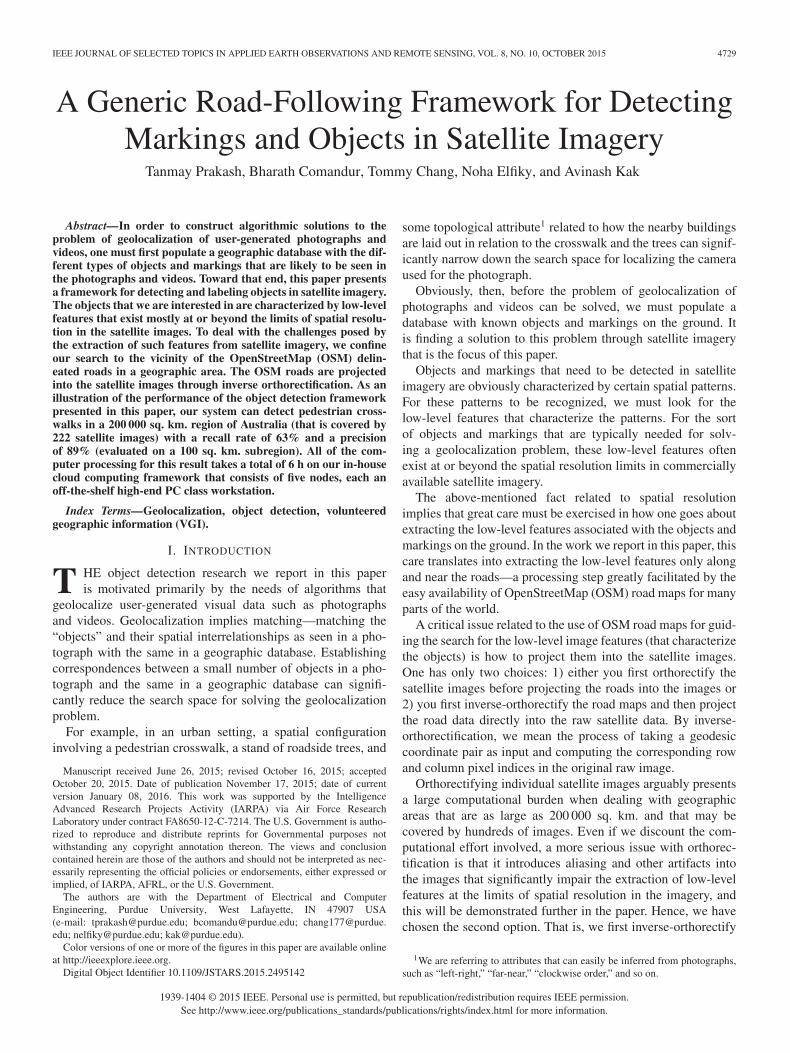
Abstract—In order to construct algorithmic solutions to theproblem of geolocalization of user-generated photographs andvideos, one must first populate a geographic database with the dif-ferent types of objects and markings that are likely to be seen inthe photographs and videos. Toward that end, this paper presentsa framework for detecting and labeling objects in satellite imagery.The objects that we are interested in are characterized by low-levelfeatures that exist mostly at or beyond the limits of spatial resolu-tion in the satellite images. To deal with the challenges posed bythe extraction of such features from satellite imagery, we confineour search to the vicinity of the OpenStreetMap (OSM) delin-eated roads in a geographic area. The OSM roads are projectedinto the satellite images through inverse orthorectification. As anillustration of the performance of the object detection frameworkpresented in this paper, our system can detect pedestrian cross-walks in a 200 000 sq. km. region of Australia (that is covered by222 satellite images) with a recall rate of 63% and a precisionof 89% (evaluated on a 100 sq. km. subregion). All of the com-puter processing for this result takes a total of 6 h on our in-housecloud computing framework that consists of five nodes, each anoff-the-shelf high-end PC class workstation.

Index Terms—Geolocalization, object detection, volunteeredgeographic information (VGI).

I. INTRODUCTION

T HE object detection research we report in this paperis motivated primarily by the needs of algorithms that

geolocalize user-generated visual data such as photographsand videos. Geolocalization implies matching—matching the“objects” and their spatial interrelationships as seen in a pho-tograph with the same in a geographic database. Establishingcorrespondences between a small number of objects in a pho-tograph and the same in a geographic database can signifi-cantly reduce the search space for solving the geolocalizationproblem.

For example, in an urban setting, a spatial configurationinvolving a pedestrian crosswalk, a stand of roadside trees, and

Manuscript received June 26, 2015; revised October 16, 2015; acceptedOctober 20, 2015. Date of publication November 17, 2015; date of currentversion January 08, 2016. This work was supported by the IntelligenceAdvanced Research Projects Activity (IARPA) via Air Force ResearchLaboratory under contract FA8650-12-C-7214. The U.S. Government is autho-rized to reproduce and distribute reprints for Governmental purposes notwithstanding any copyright annotation thereon. The views and conclusioncontained herein are those of the authors and should not be interpreted as nec-essarily representing the official policies or endorsements, either expressed orimplied, of IARPA, AFRL, or the U.S. Government.

The authors are with the Department of Electrical and ComputerEngineering, Purdue University, West Lafayette, IN 47907 USA(e-mail: [email protected]; [email protected]; [email protected]; [email protected]; [email protected]).

Color versions of one or more of the figures in this paper are available onlineat http://ieeexplore.ieee.org.

Digital Object Identifier 10.1109/JSTARS.2015.2495142

some topological attribute1 related to how the nearby buildingsare laid out in relation to the crosswalk and the trees can signif-icantly narrow down the search space for localizing the cameraused for the photograph.

Obviously, then, before the problem of geolocalization ofphotographs and videos can be solved, we must populate adatabase with known objects and markings on the ground. Itis finding a solution to this problem through satellite imagerythat is the focus of this paper.

Objects and markings that need to be detected in satelliteimagery are obviously characterized by certain spatial patterns.For these patterns to be recognized, we must look for thelow-level features that characterize the patterns. For the sortof objects and markings that are typically needed for solv-ing a geolocalization problem, these low-level features oftenexist at or beyond the spatial resolution limits in commerciallyavailable satellite imagery.

The above-mentioned fact related to spatial resolutionimplies that great care must be exercised in how one goes aboutextracting the low-level features associated with the objects andmarkings on the ground. In the work we report in this paper, thiscare translates into extracting the low-level features only alongand near the roads—a processing step greatly facilitated by theeasy availability of OpenStreetMap (OSM) road maps for manyparts of the world.

A critical issue related to the use of OSM road maps for guid-ing the search for the low-level image features (that characterizethe objects) is how to project them into the satellite images.One has only two choices: 1) either you first orthorectify thesatellite images before projecting the roads into the images or2) you first inverse-orthorectify the road maps and then projectthe road data directly into the raw satellite data. By inverse-orthorectification, we mean the process of taking a geodesiccoordinate pair as input and computing the corresponding rowand column pixel indices in the original raw image.

Orthorectifying individual satellite images arguably presentsa large computational burden when dealing with geographicareas that are as large as 200 000 sq. km. and that may becovered by hundreds of images. Even if we discount the com-putational effort involved, a more serious issue with orthorec-tification is that it introduces aliasing and other artifacts intothe images that significantly impair the extraction of low-levelfeatures at the limits of spatial resolution in the imagery, andthis will be demonstrated further in the paper. Hence, we havechosen the second option. That is, we first inverse-orthorectify

1We are referring to attributes that can easily be inferred from photographs,such as “left-right,” “far-near,” “clockwise order,” and so on.

1939-1404 © 2015 IEEE. Personal use is permitted, but republication/redistribution requires IEEE permission.See http://www.ieee.org/publications_standards/publications/rights/index.html for more information.

4730 IEEE JOURNAL OF SELECTED TOPICS IN APPLIED EARTH OBSERVATIONS AND REMOTE SENSING, VOL. 8, NO. 10, OCTOBER 2015

the OSM road data and then project them into the raw satelliteimages.

As a consequence, our overall problem of object detectionin satellite images boils down to the following: 1) inverse-orthorectify the OSM roads into the satellite images; 2) scanthe roads in the images with a search window that straddlesthe OSM roads, the search window being sufficiently wide tocompensate for any registration errors associated with project-ing the roads into the images; and 3) invoke the computer visionalgorithms for extracting the low-level features that define theobjects of interest.

This paper presents a generic solution to the problem asstated above. Our solution is generic in the sense that its front-end—which consists of inverse-orthorectification of the roadmaps, projecting these roads into the images, and scanningalong the roads—remains the same for the different types ofobjects for which we want to create a detection algorithm. Theonly part that changes from one object type to another is thecomputer vision module that is applied to the pixels in thesearch window.

Our paper presents two applications of this generic road-following framework for object detection: detecting pedestriancrosswalks and linear trees in large geographic areas. When wesay large, we mean geographic areas that may be as large as200 000 sq. km. in area and that are covered by hundreds ofsatellite images.

Requiring our detection framework to work over large geo-graphic areas implies that any decision thresholds we use in ourcomputer vision algorithms cannot be fine-tuned to individualsatellite images. Therefore, any detection performance numberswe present must be seen against a background of this fact.

To give a reader a brief preview of the sort of performancenumbers we are talking about, our system can detect pedestriancrosswalks from the satellite images of a 200 000 sq. km. regionof interest (ROI) in Australia with a recall rate of 63% and aprecision of 89%.

This paper is organized as follows. Section II presents a briefreview of the relevant literature. Section III then presents a briefdescription of the satellite data we have used in our experimen-tal work. Section IV presents the road-following framework thatunderlies the pedestrian crosswalk and linear trees detectors wepresent subsequently in Sections V and VI. The experimentalresults are presented in Section VII. Finally, we conclude inSection VIII.

II. RELATED LITERATURE

A great deal of work has been done in extracting objects fromremote sensing imagery, but the objects targeted have rarelybeen useful to the task of geolocalizing user-generated visualdata. Much of the object detection literature has focused onbuildings [1]–[4], roads [3], [5]–[7], and vehicles [8]–[17].

The work presented in [18] is one of the few to address roadmarking detection. The overall goal is actually road extrac-tion, but it does include a crosswalk detector as a means ofimproving the road extraction. Their crosswalk detector appliesmorphological operators to a segmented image in order tocreate blobs, and then accepts blobs as crosswalks based on

size and shape. Unlike our approach, their work makes nouse of the striped pattern of a crosswalk. Furthermore, theirwork presents no quantitative analysis of the detection results,making comparisons difficult.

There has been some work in the past on the detection oftrees and forests in general [19], [20]. The contribution in [19]requires very close range photography as it is based on theassumption that inter-pixel distances are of the order of 30 cmat most. The contribution in [20] models the treetops as circu-lar clusters of pixels and then estimates the presence of thoseclusters and their associated radii by scale-space analysis of theNDVI values. The authors have shown their results on two time-lapsed satellite images to demonstrate the effectiveness of theiralgorithm. We believe that scale-space analysis, while ideal forprocessing an entire satellite image all at once, would be inap-propriate for a road-following-based tree detector in which onlythose pixels that are on or in the vicinity of roads are examined.

It should also be noted here that crosswalks and linear treesare included in OSM under the tags, “crossing” and “treerow.” However, these tags show up very infrequently in allof geographic areas we have looked at. Additionally, the tag“crossing” may also be used in OSM to indicate a pedestrianwalkway delineated by two parallel lines perpendicular to theroad—an object that is not of any interest to us.

Since our paper deals with object detection on or in the vicin-ity of the roads, and since there have been past contributions onvehicle detection in satellite imagery, here we cite those con-tributions that are relevant to our work. In general, the stepsinvolved in vehicle detection consist of two stages: 1) featureextraction and 2) machine learning [8]–[17]. The features thathave been investigated include: 1) Haar-like features [9], [12];2) histogram of oriented gradients [8], [9]; and 3) local binarypatterns [9]. The machine learning techniques used include:1) adaptive boosting [9], [12]; 2) partial least squares for dimen-sionality reduction [8]; 3) support vector machines [8]; 4) linearand quadratic discriminant analysis [11]; and 5) morphologicalshare-weight neural networks (MSNN) [10].

The work described in [8] creates a two-stage cascade ofSVM classifiers to detect vehicles. The initial feature set con-sists of 70 000 dimensions, but using partial least squares fordimensionality reduction, and ordered predictors selection forfeature selection, the descriptor is reduced to a much lowerdimension before the SVM classifiers are trained. The workpresented in [10] creates a classifier using MSNN, which isessentially a linear shared-weight neural network where thefeatures are morphological. In the work described in [12], theauthors detect individual vehicles using a classifier trained byadaptively boosting Haar-like features, as well as queues ofvehicles using a line extraction technique. Additional individ-ual vehicles can then be extracted from the vehicle queues.In the work described in [17], the authors use morphologicaloperations to detect vehicles against light or dark backgrounds.

With regard to the relationship of the road-following aspectof our work to how road networks have been used in the past,many vehicle detection and traffic flow estimation algorithmsmake use of GIS road network data [12]–[16]. The road-following approach described in [13], meant for helicopter-based overhead imagery, is similar to ours in that their approach

PRAKASH et al.: GENERIC ROAD-FOLLOWING FRAMEWORK FOR DETECTING MARKINGS AND OBJECTS 4731

extracts windows along the road and rotates the windows toa canonical orientation. However, in addition to using high-quality images recorded at low altitudes, their work usesorthorectified images, rather than raw images. As we have men-tioned, and as we will discuss further, orthorectification canintroduce aliasing artifacts and a slight loss of resolution thatcan hinder algorithmic detection of objects whose features areat the limits of spatial resolution.

We should also mention that in contrast with how road net-works have been used by other authors in the past, we focus notonly on the road pixels per se, but also on the pixels in the vicin-ity of the roads. Some of the objects and the markings we areinterested in are not on the roads themselves, but on the sidesof the roads. This distinction is important, because it meansour detectors must handle a variety of clutter that is greaterthan what is seen on just the roads. At the same time, usinga processing window larger than the width of a road means anobject detector is less likely to miss the targets because of anymisalignment between the OSM roads and the images.

III. SATELLITE DATA USED IN OUR EVALUATION

OF OBJECT DETECTORS

For the purpose of this study, satellite images are drawn fromtwo large ROIs, one covering a 200 000 sq. km. area in thesoutheast of Australia and the other covering a 10 000 sq. km.area in the west coast of Taiwan. The former are panchromaticimages at a spatial resolution of 0.4− 0.5 m per pixel takenby the GeoEye-1 satellite, whereas the latter are pansharpenedimages at a similar spatial resolution obtained from Worldview-2 satellite images. The pansharpening was performed using theOrfeo Toolbox [21]. From the corresponding OSM layers, weextract only major roads and exclude smaller service roads.As demonstrated in later sections, our road guided frameworkmakes it easy to incorporate intelligent search strategies to elim-inate many possible sources of confusion to the object detectorsas well as to handle the issues of scalability to big data. Workingwithin this framework, our detectors take only a few hours torun across these large ROIs using just a five-node cluster ofPC-class machines.

IV. ROAD-FOLLOWING FRAMEWORK

As mentioned in Section I, we are only interested in detectingobjects along and in the vicinity of the roads in large geographicregions. The road maps we use in our detection framework arethose made available by OSM.2 OSM is vector data. By that, wemean that each road segment is represented by its endpoints ingeodesic coordinates. Therefore, to utilize the two data sourcestogether—OSM road maps and the satellite images—we firstneed to bring them to a common coordinate system.

The traditional approach to this coregistration of a satel-lite image with the OSM roads involves orthorectification ofthe satellite image using algorithms that are now fairly stan-dardized [22]. These algorithms convert the image from an

2In order to extract the OSM vectors relevant to a satellite image, for eachsatellite image that covers any portion of a geographic ROI, we use the latitudeand longitude offsets associated with the image along with its pixel resolutionand dimensions to segment out the corresponding part from OSM.

array defined with pixel coordinates to an array defined withlat/long coordinates. Subsequently, the OSM roads can be pro-jected straightforwardly into the orthorectified images using thegeodesic coordinates of the end points of the road segments.However, the interpolation and other approximations associatedwith converting an array of pixel coordinates into an array oflat/long coordinates lead, in general, to a slight loss of spatialresolution and possibly aliasing artifacts in the orthorectifiedimages.3 We will visually illustrate the loss of resolution andthe aliasing artifacts on a portion of a satellite image later inthis section. For most applications of satellite imagery, the arti-facts and the loss of resolution are not noticeable. However,in our case, when the objects and the markings we are look-ing for possess low-level features that are at very low spatialresolutions (near 0.5 m), such artifacts can significantly impairdetector performance.

It is important to note that the loss of information due toorthorectification cannot be prevented by merely upsamplingor using different resampling techniques. As an illustration ofthe effects of orthorectification in Section VII-A, the recall andprecision of the crosswalk detector both drop by nearly 20%when orthorectified images are used.

Hence, in this paper, we use the other approach to the co-registration of a satellite image with OSM—the approach basedon inverse-orthorectification. Since inverse orthorectificationdoes not involve directly manipulating the pixels in a satelliteimage, it does not result in the aliasing artifacts and the res-olution loss. Inverse orthorectification is also computationallymuch faster since now there is no need to process all the pixelsin all the satellite images for a given ROI. Inverse orthorecti-fication requires us to only project the OSM vector endpointsinto the raw satellite images—the images themselves need notbe modified in any manner. As those familiar with orthorec-tification would guess, the inverse orthorectification processalso uses rational polynomial coefficients (RPCs) and the DEMthat correspond to a particular satellite image. The RPC equa-tions shown below model the pixel coordinates as ratios ofpolynomials over the geodesic coordinates [22]

rn =frNum(φn, λn, hn)

frDen(φn, λn, hn)

, cn =f cNum(φn, λn, hn)

f cDen(φn, λn, hn)

(1)

where each f is a different cubic polynomial in φ, λ, and h with20 coefficients and where

φn =φ− φoffset

φscale, λn =

λ− λoffset

λscale, hn =

h−hoffset

hscale

rn =r − roffset

rscale, cn =

c− coffsetcscale

. (2)

In the above equations, φ, λ, and h denote the latitude, lon-gitude, and height coordinates for a given geolocation. Thevariables r and c denote the corresponding pixel row and col-umn values. The offsets and the scale factors are provided

3The formulas that convert pixel coordinates of the raw satellite images intolat/long coordinates utilize a digital elevation map (DEM) model of the portionof the earth’s surface that corresponds to the satellite image. These formulasare iterative and involve various approximations for warping the image dataonto the earth’s surface, in addition to the interpolation needed to create a uni-formly sampled array in the lat/long coordinates. The errors in orthorectificationcomputations are exacerbated by any errors in the DEM model. Typical DEMmodels are at 30 m resolution.


Fig. 1. Inverse-ortho means that we are directly using the raw image. Orthomeans that the image is rectified into a lat/long array which entails a slightloss of resolution and introduces additional aliasing artifacts. (a) Ortho.(b) Inverse-ortho. (c) Ortho (crosswalk magnified). (d) Inverse-ortho (crosswalkmagnified).

together with the RPC coefficients in the metadata associatedwith a satellite image. It is possible to use just the RPC-basedequations without DEM by assuming an average elevationfor the earth’s surface covered by a satellite image. However,using height information from the DEM reduces the errors inprojection.

For each road segment, we use the equations shown above toproject the geodesic coordinates of the OSM vector endpointsinto the raw satellite images.

Now that we have made clear what we mean by inverseorthorectification, it is time to illustrate how the “quality” of asatellite image at the limits of its spatial resolution can dete-riorate by orthorectification. Figs. 1(a) and (b) are the sameportions of a satellite image; the one in (a) is orthorectified andthe one in (b) corresponds to inverse orthorectification (mean-ing what is shown is the raw image patch itself). Figs. 1(c) and(d) show just the crosswalk portions of the image patches in(a) and (b), respectively. Notice how the crosswalk strips in theorthorectified images in (a) and (c) suffer from a strong stair-case effect due to image aliasing, vis-a-vis how they show up in(b) and (d).4

Once the two data sources are combined through inverseorthorectification, we can use the road network to guide ourdetectors. This is described as follows.

4If the reader would indulge us by viewing the four images in Fig. 1 froma distance, he/she will notice a relatively strong semblance of crosswalk stripsin the two images in the right column. However, the same strips in the twoimages in the left column have a strong staircase effect caused by image alias-ing. This staircase effect can make it more difficult to detect periodicities whenthe contrast differences are low.

Fig. 2. Rotating the road to align with the vertical axis.

A. Road-Following Algorithm

Our object detectors use a moving window approach forextracting spatial and spectral features. A normal pixel-basedapproach to object detection on (and in the vicinity of) the roadswould be to carry out a rectilinear scan of an image and centera search window at each road pixel. Instead, we use a moreefficient approach in which the search window moves alongthe road segments, one segment at a time.5 The road-followingalgorithm consists of the following steps.

1) Interpolate between the two endpoints of a road segmentand select fixed points along the road as center points forthe window.

2) The spacing between two successive points on a roadsegment (for placing the search window) depends on theobject in question and the dimensions of the window. Weensure that there is sufficient overlap between successiveplacements of the search window so as not to miss thetarget object.

3) Since we know the actual geographic orientation of theroad, we rotate the search window at each location sothat, from the standpoint of computer processing, theroad is aligned along the vertical axis. We use Lanczosinterpolation [23], [24] to obtain a smooth rotation.

An important consequence of Step 3) is that it makes iteasier to write the computer vision code for detecting objectsin the search window. In general, how an object is orientedwith respect to a road influences the logic of how an object isdetected vis-a-vis the road. Orienting the road vertically elimi-nates at least one degree-of-freedom in the prescription of thatlogic. Fig. 2 shows an example of this step.

Obviously, any misregistration between the OSM data andthe satellite imagery will propagate into our framework.However, choosing appropriate dimensions for the searchwindow can mitigate the effects of small to moderate misreg-istration errors to a significant extent—as demonstrated by ourresults.

5More specifically, OSM is clipped according to the lat/long coordinatescorresponding to a given satellite image. What one gets from such a clippedregion is a list of straight road segments, with each segment defined by its twoendpoints. Our road scanner scans through each item in this list.


B. Cloud-Based Processing

For fast processing speeds, the road-following framework,along with the logic of the detectors presented in Sections Vand VI, runs in parallel on our in-house cloud computingcluster called the RVL-Cloud. This cluster consists of five high-performance physical nodes, each with up to 48 cores and256 GB of RAM. A 36-TB network attached storage connectedto the cloud contains all the satellite images for the datasetsmentioned in Section III. In general, an ROI may be cov-ered by hundreds of satellite images. Multiple virtual machines(VMs) are used to process all relevant satellite images, witheach VM processing one image at a time. Since each VMis assigned dozens of cores, a given VM further parallelizesthe task by chopping a large image into smaller sections, anddistributing the sections among multiple processes, with eachprocess running in a separate core.

We now present two object detectors that have been imple-mented by incorporating specially designed computer visionmodules into the road-following framework described so far.

V. PEDESTRIAN CROSSWALK DETECTOR

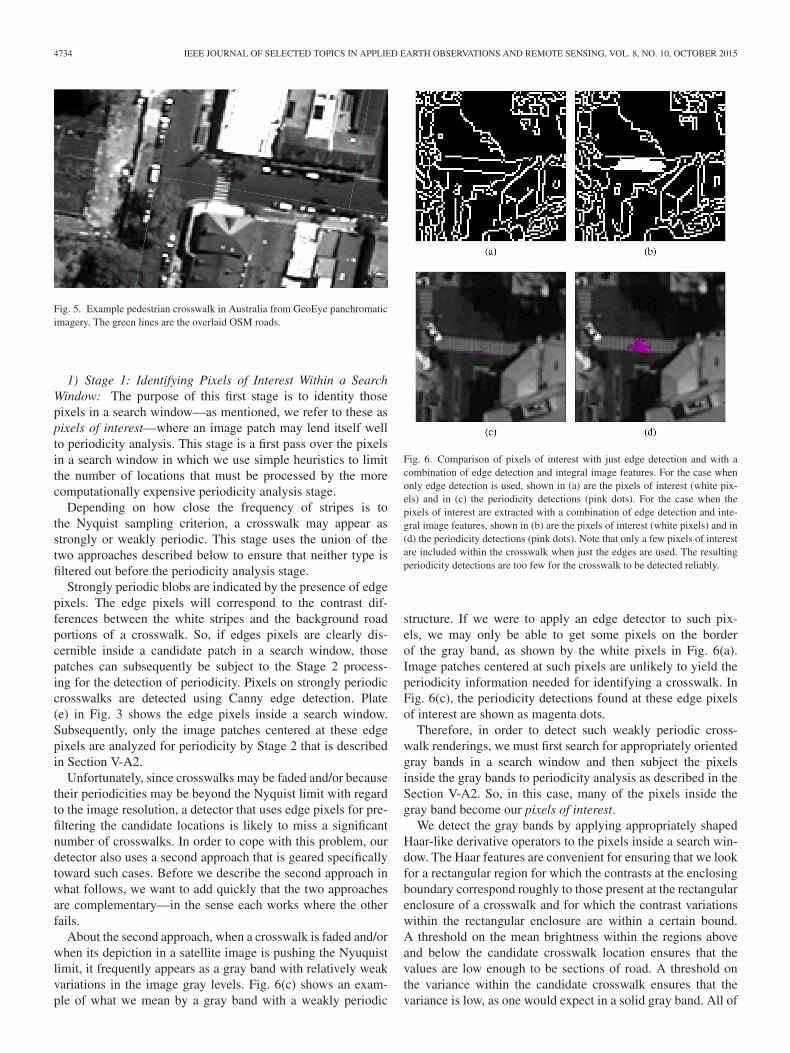
Typically, a pedestrian crosswalk appears in a satellite imageas a rectangular portion of a road that contains pixels corre-sponding to the black and white stripes of the crosswalk. Anexample of a crosswalk is shown in Fig. 5. When such pixelsare reliably sensed, the striped pattern exhibits a periodicity thatis a fairly discriminative feature which can be leveraged by thecrosswalk detector.

Since this detector is expected to work over large geographicareas that may be covered by hundreds of satellite images, therecan be significant variation in how the pixels corresponding toa crosswalk appear in the images. Another complicating fac-tor relates to the spatial resolution in the images. It is oftenthe case that each stripe of a crosswalk is sampled by just onepixel.6 This makes it difficult to estimate the periodicities asso-ciated with the pixels that fall on a crosswalk. Additionally,many crosswalks that have been subject to much traffic withoutrepainting can appear faded. Occlusions from cars and trees canfurther confound detection. All of these are reasons for why anactual crosswalk on the ground may not be detectable as such ina satellite image. On the other side of the coin, we also have sit-uations when noncrosswalk blobs of pixels may be detected ascrosswalks. For example, rows of windows on buildings, linesof cars in parking lots, lane markings on wide roads, etc., allpresent high degrees of periodicity that may be mistaken forcrosswalks if they appear inside a search window.

A. Crosswalk Detection Algorithm

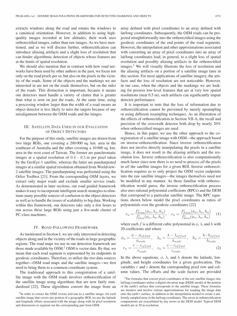
The pedestrian crosswalk detector involves a cascade of threestages, with the first stage choosing pixels of interest fromwithin a search window where one should test for periodicity,the second stage applying a periodicity detector to the imagepatches centered at the pixels of interest, and the third stage

6When the sampling rate falls below one-pixel per stripe (as does occur insome regions of the world), the Nyquist limit is violated, which injects aliasingnoise into the estimation of the periodicities.

Fig. 3. Flowchart illustrating our road-following framework, as well as thedownstream crosswalk detector. (e) Pixels of interest stage: Extract pixels thatmay fall on a crosswalk. (f) Periodicity analysis stage: Analyze pixels of interestfor periodicity, culling those without significant periodicity. (g) Agglomerationstage: Agglomerate periodic pixels into groups, and use size and orientation tofilter groups.

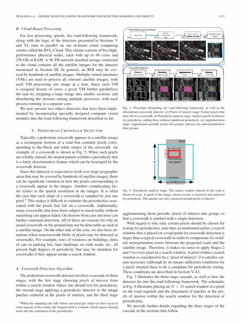
Fig. 4. Periodicity analysis stage. The search window placed on the road isshown in cyan. A patch of the image, shown in red, is extracted and analyzedfor periodicity. The patches are only extracted around pixels of interest.

agglomerating those periodic pixels of interest into groups sothat a crosswalk is marked with a single detection.

With regard to why only certain pixels should be chosen fortesting for periodicities, note that, as mentioned earlier, a searchwindow that is placed on a road point for crosswalk detection islarger than a typical crosswalk in order to compensate for resid-ual misregistration errors between the projected roads and thesatellite image. Therefore, it makes no sense to apply Stages 2and 3 to every pixel in a search window. A pixel within a searchwindow is considered to be a “pixel of interest” if it satisfies cer-tain necessary (although by no means sufficient) conditions fora patch situated there to be a candidate for periodicity testing.These conditions are described in Section V-A1.

Fig. 3 illustrates the three-stage cascade, as well as how thedetector fits into the road-following framework. The schematicin Fig. 4 illustrates placing an M ×M search window at a pointon the road segment and the placement of patches at the pix-els of interest within the search window for the detection ofperiodicities.

We provide further details regarding the three stages of thecascade in the sections that follow.


Fig. 5. Example pedestrian crosswalk in Australia from GeoEye panchromaticimagery. The green lines are the overlaid OSM roads.

1) Stage 1: Identifying Pixels of Interest Within a SearchWindow: The purpose of this first stage is to identity thosepixels in a search window—as mentioned, we refer to these aspixels of interest—where an image patch may lend itself wellto periodicity analysis. This stage is a first pass over the pixelsin a search window in which we use simple heuristics to limitthe number of locations that must be processed by the morecomputationally expensive periodicity analysis stage.

Depending on how close the frequency of stripes is tothe Nyquist sampling criterion, a crosswalk may appear asstrongly or weakly periodic. This stage uses the union of thetwo approaches described below to ensure that neither type isfiltered out before the periodicity analysis stage.

Strongly periodic blobs are indicated by the presence of edgepixels. The edge pixels will correspond to the contrast dif-ferences between the white stripes and the background roadportions of a crosswalk. So, if edges pixels are clearly dis-cernible inside a candidate patch in a search window, thosepatches can subsequently be subject to the Stage 2 process-ing for the detection of periodicity. Pixels on strongly periodiccrosswalks are detected using Canny edge detection. Plate(e) in Fig. 3 shows the edge pixels inside a search window.Subsequently, only the image patches centered at these edgepixels are analyzed for periodicity by Stage 2 that is describedin Section V-A2.

Unfortunately, since crosswalks may be faded and/or becausetheir periodicities may be beyond the Nyquist limit with regardto the image resolution, a detector that uses edge pixels for pre-filtering the candidate locations is likely to miss a significantnumber of crosswalks. In order to cope with this problem, ourdetector also uses a second approach that is geared specificallytoward such cases. Before we describe the second approach inwhat follows, we want to add quickly that the two approachesare complementary—in the sense each works where the otherfails.

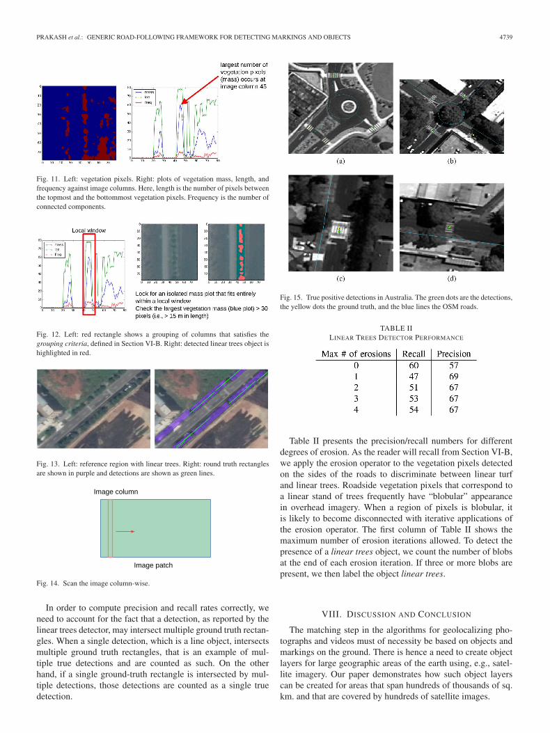
About the second approach, when a crosswalk is faded and/orwhen its depiction in a satellite image is pushing the Nyuquistlimit, it frequently appears as a gray band with relatively weakvariations in the image gray levels. Fig. 6(c) shows an exam-ple of what we mean by a gray band with a weakly periodic

Fig. 6. Comparison of pixels of interest with just edge detection and with acombination of edge detection and integral image features. For the case whenonly edge detection is used, shown in (a) are the pixels of interest (white pix-els) and in (c) the periodicity detections (pink dots). For the case when thepixels of interest are extracted with a combination of edge detection and inte-gral image features, shown in (b) are the pixels of interest (white pixels) and in(d) the periodicity detections (pink dots). Note that only a few pixels of interestare included within the crosswalk when just the edges are used. The resultingperiodicity detections are too few for the crosswalk to be detected reliably.

structure. If we were to apply an edge detector to such pix-els, we may only be able to get some pixels on the borderof the gray band, as shown by the white pixels in Fig. 6(a).Image patches centered at such pixels are unlikely to yield theperiodicity information needed for identifying a crosswalk. InFig. 6(c), the periodicity detections found at these edge pixelsof interest are shown as magenta dots.

Therefore, in order to detect such weakly periodic cross-walk renderings, we must first search for appropriately orientedgray bands in a search window and then subject the pixelsinside the gray bands to periodicity analysis as described in theSection V-A2. So, in this case, many of the pixels inside thegray band become our pixels of interest.

We detect the gray bands by applying appropriately shapedHaar-like derivative operators to the pixels inside a search win-dow. The Haar features are convenient for ensuring that we lookfor a rectangular region for which the contrasts at the enclosingboundary correspond roughly to those present at the rectangularenclosure of a crosswalk and for which the contrast variationswithin the rectangular enclosure are within a certain bound.A threshold on the mean brightness within the regions aboveand below the candidate crosswalk location ensures that thevalues are low enough to be sections of road. A threshold onthe variance within the candidate crosswalk ensures that thevariance is low, as one would expect in a solid gray band. All of


these features can be calculated quickly using an integral imagerepresentation of the pixels inside the search window [25].

Finally, from the pixels of interest derived from bothmethods—the edge-based pixels of interest and the Haar-basedpixels of interest—we delete those where the brightness levelsfall below a threshold. This ensures that they do not fall on areasthat are too dark to be crosswalks, like asphalt.

2) Stage 2: Periodicity Analysis Stage: In this stage, weconsider a patch around each pixel of interest returned by thefirst stage for periodicity analysis. The goal is to select justthose pixels of interest where the periodicity is sufficientlystrong.

Given a pixel of interest returned by Stage 1, the periodic-ity detector first extracts a p× q patch centered at that pixel.It then sums the pixel values along the vertical columns of thepatch, creating a one-dimensional (1-D) p-sample signal. Thisintegration along the road suppresses some of the noise, whilemaintaining the periodicity of the crosswalk stripes that are typ-ically perpendicular to the road. The periodicity detector thencalculates the discrete Fourier transform of the 1-D p-samplesignal.

Two different thresholds are applied to the calculated 1-DFourier transform: 1) one for the frequency and 2) the other forthe magnitude of the transform itself at the selected frequen-cies. Through our prior knowledge about pedestrian crosswalksgenerally, and also our prior knowledge of spatial resolution in asatellite image, we know that, for valid patches, the peaks in the1-D discrete Fourier transform must occur close to the highestfrequency for which the DFT is calculated. We can, therefore,choose a frequency below which we can simply ignore theoutput of the Fourier transform calculator.

The second threshold is related to the magnitude of the peakin the frequency window that is let through by the first thresh-old. If the magnitude falls below this threshold, the peak is tooweak for the patch to be considered periodic. This threshold isset relative to the maximum magnitude in the DFT, excludingthe dc component. This allows the threshold to adapt to dif-ferent illuminations (as caused by different sun angles, cloudcover, etc.). However, we do not allow the threshold to fallbelow a certain value; this suppresses those cases when themaximum magnitude is very low, as might happen when thevariation in the patch is just noise.

Note that at this point, a single crosswalk is likely to bemarked by multiple periodic pixels. For convenience, we referto those pixels of interest where periodicity is detected asperiodic pixels.

3) Stage 3: Agglomeration Stage: This stage not onlygroups together those periodic pixels that mark the same cross-walk, but also filters out false positives. Unlike the other twostages, which process one search window at a time, the agglom-eration stage processes the periodic pixels from all the searchwindows in a given satellite image all at once. This stageagglomerates the periodic pixels into clusters, which can befurther filtered.

The agglomeration proceeds by first creating a binary imagefor the entire satellite image, with all the periodic pixels setto 1. Subsequently, this binary image is subject to a movingwindow aggregation with a disk-shaped window. By this, we

Fig. 7. Typical strips of roadside trees (circled in the red ovals) in Taiwan. Thebottom image is the overhead view of the same trees shown in the top image.Image sources: Google Street View and Google Maps.

simply mean that we place a disk-shaped window at every loca-tion in the image, find the number of pixels set to 1 within thewindow, and return the resulting total as the output value at thatlocation. By applying a threshold Ngroup to this output, smallspurious groups of periodic pixels are removed. We discuss howto choose the value of Ngroup in Section VII. The next stepis to find the connected components of the thresholded image.Each connected component serves as a mask that contains allthe periodic pixels in a cluster.

The detector finally filters the clusters based on their orien-tation with respect to the road. True crosswalks are, with a fewexceptions, oriented at 90◦ to the road, where the angle is mea-sured between the line perpendicular to the crosswalk stripesand the line along the center of the road. We find the orientationof the cluster by carrying out a principal components analysis(PCA) of the coordinates of the periodic pixels within the clus-ter. The angle of the cluster is calculated as that between theeigenvector with the largest eigenvalue, and the road throughthe cluster. If this angle falls below a threshold, the cluster isrejected. However, if the ratio of the eigenvalues is too closeto 1, it implies that the angle measurement may not be accu-rate enough to warrant rejection. The centers of the acceptedclusters are reported as the final crosswalk detections.

This marks the end of our presentation of the pedestriancrosswalk detector. We next describe the application of ourgeneric road-following object detector to the case of detectinglinear stands of trees along the roads.

VI. LINEAR TREES DETECTOR

In this section, we describe roadside tree detection as anotherapplication of our road-based object detection framework.Specifically, we use the framework to detect roadside trees thatare arranged in a linear fashion. Fig. 7 shows two typical stripsof roadside trees. We refer to such formations of roadside treesas linear trees in the rest of the paper.

For the purpose of designing a computer vision algorithm fortheir detection, a linear trees object is defined as a collection of


roadside vegetation pixels that satisfy the following two prop-erties. 1) The pixels are bounded by a box that satisfies certainminimum constraints with regard to its length along the roadand width perpendicular to it. Typically, we would want thebounding box for a linear trees object to possess a width that isbetween 2 and 4 m and a length greater than 20 m. 2) The pixelblob within the bounding box possesses a “blobular” shape.The shape property is necessary to separate a stand of treesfrom a uniform run of turf that is frequently found along majorhighways. We will detect the “blobular” property by apply-ing erosion operators to the vegetation pixels to see if we endup with disconnected blobs. If a small number of erosions donot result in disconnected blobs, it is more likely that we arelooking at linear turf along the road.

The computer vision algorithm that extracts such pixel for-mations consists of the following four steps.

1) Identify roadside vegetation pixels in the satellite image.2) Sum the vegetation mass along the columns (meaning, in

directions parallel to the road) and extract the width of thevegetation pixels perpendicular to the road.

3) Construct bounding boxes for the vegetation pixel blobs.4) Apply erosion operators to the vegetation pixel blobs to

identify the linear tree blobs.We describe these steps in the next two sections.

A. Identify Vegetation Pixels

There does not exist sufficient information in the multispec-tral signatures in the satellite data that would allow for pixelsto be directly identified as tree pixels. However, we can extractvegetation pixels along the roads fairly reliably. These vegeta-tion pixels are subsequently subject to blob analysis for them tobe labeled as tree pixels.

There exist the following two solutions to the identificationof vegetation pixels.

1) Through the normalized difference vegetation index(NDVI) characterization of a pixel. NDVI is computedusing the red and the near infrared (NIR) spectral bandsand is thus effective at detecting vegetation. It has beenshown that NDVI is directly related to the photosyntheticcapacity of plant canopies [26]. The formula for NDVI is

NDVI =NIR − REDNIR + RED

.

2) Through the visible atmospherically resistant index(VARI) characterization of a pixel. VARI is used to com-pute an approximation to vegetation fraction (VF) inthe multispectral data [27]. Unlike NDVI, VARI doesnot need infrared and can be computed from the com-monly available red, green, and blue visible spectralbands through the following formula:

VARI =GREEN − RED

GREEN + RED − BLUE.

In this paper, we say that a pixel is a vegetation pixel if itsNDVI value exceeds some threshold Vthres. The resulting veg-etation segmentation is a binary image in which the foreground

consists of vegetation pixels. We discuss how to choose a valuefor Vthres in Section VII.

In general, NDVI values are high for all types of green veg-etation including grasslands, shrubs, forests, and so on. Ourblob and peak-value analysis described in Section VI-B elim-inates many of these sources of high NDVI values. However,this analysis allows linear shrubs to be mistaken for linear tress.We consider those as examples of false positives.

B. Identify Narrow Strips of Tree Pixels

The logic for identifying narrow “blobular” strips of vegeta-tion that would subsequently be labeled as linear trees is madeparticularly simple by the fact that, for the purpose of computerprogramming, our road-following framework always keeps theroad vertical. This means that all we need to do is to examinethe pixels within certain narrow columns on the two sides of aroad and characterize what we find in those columns. No inter-polation need be carried out for this column-based processingsince all the pixels with the same column index belong to a sin-gle one-pixel wide strip parallel to the road. The question thenbecomes whether such column-based logic that makes infer-ences on the basis of the contents of multiple adjacent columnsis feasible in the presence of residual registration errors betweenthe OSM roads and the road pixels as they show up in thesatellite images. Our results show that the trees can indeed beidentified with usable levels of accuracy despite the registrationerrors.

To describe this column-based processing as applied to asearch window, the portion of the image within the windowis scanned one column at a time. For each column, we countthe number of vegetation pixels in the column (See Fig. 14.).We then sort and visit the columns in decreasing order of thesecounts. For each column visited, we group the column with itsneighboring columns on both sides when the grouping criteriadescribed below are met.

However, before we describe the grouping criteria, we firstdefine the following terms.

1) mass(x): number of vegetation pixels in the image col-umn x.

2) col: column index for a column with a high mass value.3) r: maximum expected radius of the trees.4) colL: the column that is positioned r columns to the left

of col.5) colR: the column that is positioned r columns to the right

of col.The grouping criteria that have worked the best based on our

experiments are1) mass(col) > Mthres;2) mass(colL) < 0.5×mass(col);3) mass(colR) < 0.5×mass(col).The purpose of Criteria 2 and 3 is to make sure that the

boundary columns are near the edges of the vegetation strip ifit is to be accepted as a tree strip. In other words, we do notexpect many tree pixels outside the tree strip.

The group of columns from colL to colR will, in general,constitute a vegetation region. In order to label this region asa stand of trees, its shape along the road must be blobular—a


shape characterization that can be determined by an iterativeapplication of an erosion operator to the pixels. The numberof applications of the erosion operator and the number of dis-connected blobs one should expect for the linear trees label areexperimental parameters that we will present in Section VII.

That brings to an end our presentation of the essential ele-ments of the detector for linear trees objects. Section VIIpresents results on the performance of the crosswalk and thelinear trees detectors on large ROIs.

VII. EXPERIMENTS

As mentioned in Section I, we started with the goal ofcreating object detectors that could be applied to possibly hun-dreds of satellite images covering large geographic ROI’s. Ourunderlying motivation was to be able to detect objects thatcould subsequently be used for the geolocalization of pho-tographs and videos. Since the objects we are interested inpossess features at the limits of spatial resolution in the avail-able imagery, we decided to create road-based detectors (sincethe photographs and videos are highly likely to be recordedfrom locations on or in the vicinity of the roads anyway).

As our experimental results in this section demonstrate,detectors based on road-following logic possess usable perfor-mance despite the image-to-image variability in the satellitedata and despite the fact that the low-level features represent-ing the objects of interest (say, the crosswalks) are at the limitsof spatial resolution in the satellite data.

In what follows, we will first describe the performance of thecrosswalk detector and then that of the linear trees detector.

A. Detecting Crosswalks

As a part of IARPA’s geolocalization project, the crosswalkdetector described in Section V was applied to a 200 000 sq.km. ROI in Australia and the detected crosswalks suppliedas an object layer to our prime contractor Applied ResearchAssociates where it is being used in the development of match-ers for geolocalization of photographs and videos.

The various parameters used for the crosswalk are chosenbased on observations of the satellite data. For instance, thepatch size used for the periodicity analysis stage is set to10 m × 5 m based on the observation that most crosswalks areabout 5 m wide along the road and at least 10 m wide acrossit. The threshold on frequency is set to 0.33 cycles per pixelbased on the observation that the imaged stripe frequency variesnear the Nyquist limit of 0.5 cycles per pixel. Where intuitivedefinitions are not possible, we test various values and choosethat value that provides desirable detector performance. Fig. 8shows how the detector performance varies as the threshold ongroup size in the agglomeration stage is varied over [0, 100]detections, leading to the choice of 15 detections as the thresh-old for the baseline detector. Here, we define false positives persq. km. (FPPSK) as

FPPSK =Number of false positive detections

Ground truth area in sq. km.. (3)

Fig. 8. Recall versus false positives per sq. km. for the crosswalk detec-tor as Ngroup is varied. Ngroup is the threshold on the group size in theagglomeration stage.

To evaluate the crosswalk detector, we manually createdground truth for eight test sections in six satellite images overthe ROI.7 Each test section is rectangular with height and widthbetween 1 and 5 km. The total area of all the test sections is104.1 sq. km. A human operator generated the ground truth byvisually scanning each test section in its entirety and accept-ing a crosswalk as a part of the ground truth if its location isin the vicinity of an OSM road. This check against the OSMroads—important since our road-following framework worksoff the OSM roads—is carried out by using the QGIS open-source tool to overlay the OSM roads on the satellite images. Intotal, 142 crosswalks were found in the ground truth sections.

For measuring the performance of the detector, the number oftrue positives is calculated as the number of detections withinthe test sections for which there is a ground truth crosswalkwithin a threshold distance. The recall and precision rates aredefined as

Precision Rate =Number of true detectionsTotal number of detections

(4)

Recall Rate =Number of true detections

Number of ground truth crosswalks. (5)

Overall, the recall and precision in the test sections were 63%and 89%, respectively. Examples of true detections are shownin Fig. 15. To better understand the effect of each stage, wetested the detector performance when each stage was removedand the others kept. When the pixels of interest stage (Stage1) is removed, we instead simply apply the periodicity analysisto all running placements of 20× 10 patches with their centersfour pixels apart. When the periodicity analysis stage (Stage2) is removed, we simply pass the pixels of interest directly to

7The only constraint on the test sections was that they be in urban andsemiurban areas. This constraint was necessitated by the fact that crosswalksare relatively rare outside the urban areas. Note that crosswalk detection wasapplied to all of the satellite data covering 200 000 sq. km. It is only for theevaluation process that we limited the sections for manual groundtruthing tourban and semiurban areas.


TABLE IPEDESTRIAN CROSSWALK DETECTOR PERFORMANCE

Fig. 9. (a) Missed detections and (b,c) false positives in Australia. The greendots are the detections, the yellow dot the ground truth, and the blue lines theOSM roads.

the agglomeration stage. Finally, rather than completely remov-ing the agglomeration stage, we allowed it to form the groupsof pixels, but we removed the step that culls groups based onsize and orientation. Table I summarizes the results of theseexperiments. As the table shows, each step is important to theperformance, especially the periodicity analysis stage.

As a test of the effects of orthorectification, the detector wasalso tested on the same regions, with exactly the same parame-ters, but using orthorectified satellite images rather than the rawimages in our inverse orthorectification-based framework. Withorthorectified images, the recall and the precision were 42% and65%, respectively. These performance numbers speak for them-selves with regard to how the loss of spatial resolution and thealiasing artifacts introduced into the images by orthorectifica-tion affect the detection of features at the limit of the availablespatial resolution.

The detector misses those crosswalks that are not aligned per-pendicularly to OSM road. This can happen when the crosswalkis painted diagonally across a road, and when the OSM road isnot correctly aligned with the road in the satellite image. Oneexample of the latter case is when the crosswalk is in a curvedturn lane as in Fig. 9(a).

B. Detecting Linear Trees

As a part of the IARPA’s geolocalization project, the lineartrees detector described in Section VI was applied to a

Fig. 10. Vegetation segmentation using NDVI. Left: 40 m × 40 m road-oriented search window; Center: NDVI feature map; Right: Vegetation pixels.

10 000 sq. km. ROI in Taiwan. The detected linear trees weresupplied as an object layer to our prime contractor AppliedResearch Associates to support the development of matchersfor geolocalization of photographs and videos.

For the rest of this section, we first mention how we deter-mine the various parameters (Vthres, Mthres, and r) used inour linear trees detector. We then describe the ground truth col-lection and the evaluation protocols. Finally, we summarize thedetector performance.

Recall from Section VI-A that Vthres is used to identify veg-etation pixels from the portion of a satellite image inside thesearch window. We pick a lower bound threshold such thatmost of the vegetation pixels exceed that threshold. We havefound this value to be around 0.4. Fig. 10 shows a typical40 m × 40 m search window, its NDVI map, and the resultingvegetation segmentation.

To detect linear trees objects consisting of trees of diameterless than 7 m, we need to consider strips of width 3.5 m on bothsides of the column col. (As defined in Section VI-A, col is acandidate column with high number of vegetation pixel counts.)Since r is the number of columns on either side of col and eachpixel corresponds to 0.5 m, we set r = 3.5/0.5 = 7.

Finally, we must account for the fact that, when vegetationpixels form linear trees, there may or may not be any gapsbetween such pixel blobs along the road. To allow for both pos-sibilities, we require at least 3/8 of the total pixels in col to bevegetation pixels. Since the search window height is 80 pixels ina 40 m × 40 m search window, we set Mthres = 3/8× 80 =30.

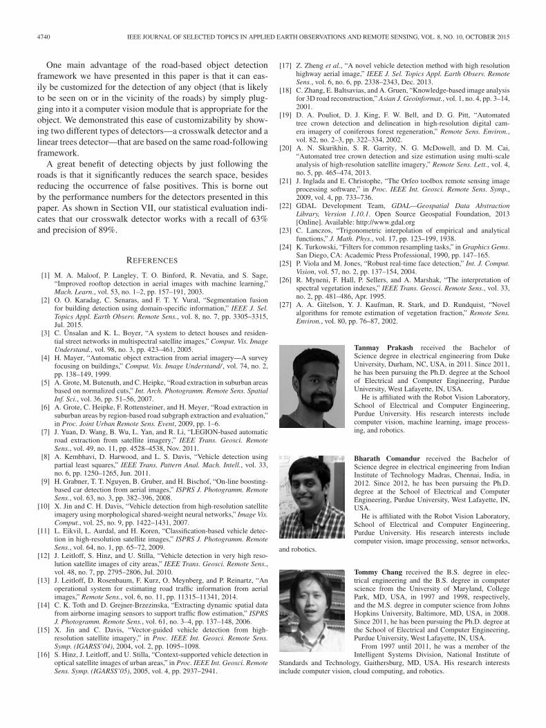
Figs. 11 and 12 demonstrate the column grouping criteriausing the parameter values mentioned. That is, Vthres = 0.4,Mthres = 30, and r = 7. Once a linear trees object is detected,we represent that detection by a geographic line consisting oftwo lat/long endpoints corresponding to the topmost and thebottommost tree pixels in col.

With regard to ground truth data, we manually annotatea 5 km × 5 km region from a typical satellite image. Theannotation process involves manually placing 5 m × 40 mnonoverlapping rectangles on top of all true linear trees. Fig. 13shows the ground truth rectangles and all the detections in asmall area.

For performance metrics, we compute precision and recallrates as follows:

Precision rate =Number of true detectionsTotal number of detections

(6)

Recall rate =Number of true detections

Number of ground truth rectangles. (7)


Fig. 11. Left: vegetation pixels. Right: plots of vegetation mass, length, andfrequency against image columns. Here, length is the number of pixels betweenthe topmost and the bottommost vegetation pixels. Frequency is the number ofconnected components.

Fig. 12. Left: red rectangle shows a grouping of columns that satisfies thegrouping criteria, defined in Section VI-B. Right: detected linear trees object ishighlighted in red.

Fig. 13. Left: reference region with linear trees. Right: round truth rectanglesare shown in purple and detections are shown as green lines.

Fig. 14. Scan the image column-wise.

In order to compute precision and recall rates correctly, weneed to account for the fact that a detection, as reported by thelinear trees detector, may intersect multiple ground truth rectan-gles. When a single detection, which is a line object, intersectsmultiple ground truth rectangles, that is an example of mul-tiple true detections and are counted as such. On the otherhand, if a single ground-truth rectangle is intersected by mul-tiple detections, those detections are counted as a single truedetection.

Fig. 15. True positive detections in Australia. The green dots are the detections,the yellow dots the ground truth, and the blue lines the OSM roads.

TABLE IILINEAR TREES DETECTOR PERFORMANCE

Table II presents the precision/recall numbers for differentdegrees of erosion. As the reader will recall from Section VI-B,we apply the erosion operator to the vegetation pixels detectedon the sides of the roads to discriminate between linear turfand linear trees. Roadside vegetation pixels that correspond toa linear stand of trees frequently have “blobular” appearancein overhead imagery. When a region of pixels is blobular, itis likely to become disconnected with iterative applications ofthe erosion operator. The first column of Table II shows themaximum number of erosion iterations allowed. To detect thepresence of a linear trees object, we count the number of blobsat the end of each erosion iteration. If three or more blobs arepresent, we then label the object linear trees.

VIII. DISCUSSION AND CONCLUSION

The matching step in the algorithms for geolocalizing pho-tographs and videos must of necessity be based on objects andmarkings on the ground. There is hence a need to create objectlayers for large geographic areas of the earth using, e.g., satel-lite imagery. Our paper demonstrates how such object layerscan be created for areas that span hundreds of thousands of sq.km. and that are covered by hundreds of satellite images.


One main advantage of the road-based object detectionframework we have presented in this paper is that it can eas-ily be customized for the detection of any object (that is likelyto be seen on or in the vicinity of the roads) by simply plug-ging into it a computer vision module that is appropriate for theobject. We demonstrated this ease of customizability by show-ing two different types of detectors—a crosswalk detector and alinear trees detector—that are based on the same road-followingframework.

A great benefit of detecting objects by just following theroads is that it significantly reduces the search space, besidesreducing the occurrence of false positives. This is borne outby the performance numbers for the detectors presented in thispaper. As shown in Section VII, our statistical evaluation indi-cates that our crosswalk detector works with a recall of 63%and precision of 89%.

REFERENCES

[1] M. A. Maloof, P. Langley, T. O. Binford, R. Nevatia, and S. Sage,“Improved rooftop detection in aerial images with machine learning,”Mach. Learn., vol. 53, no. 1–2, pp. 157–191, 2003.

[2] O. O. Karadag, C. Senaras, and F. T. Y. Vural, “Segmentation fusionfor building detection using domain-specific information,” IEEE J. Sel.Topics Appl. Earth Observ. Remote Sens., vol. 8, no. 7, pp. 3305–3315,Jul. 2015.

[3] C. Ünsalan and K. L. Boyer, “A system to detect houses and residen-tial street networks in multispectral satellite images,” Comput. Vis. ImageUnderstand., vol. 98, no. 3, pp. 423–461, 2005.

[4] H. Mayer, “Automatic object extraction from aerial imagery—A surveyfocusing on buildings,” Comput. Vis. Image Understand/ , vol. 74, no. 2,pp. 138–149, 1999.

[5] A. Grote, M. Butenuth, and C. Heipke, “Road extraction in suburban areasbased on normalized cuts,” Int. Arch. Photogramm. Remote Sens. SpatialInf. Sci., vol. 36, pp. 51–56, 2007.

[6] A. Grote, C. Heipke, F. Rottensteiner, and H. Meyer, “Road extraction insuburban areas by region-based road subgraph extraction and evaluation,”in Proc. Joint Urban Remote Sens. Event, 2009, pp. 1–6.

[7] J. Yuan, D. Wang, B. Wu, L. Yan, and R. Li, “LEGION-based automaticroad extraction from satellite imagery,” IEEE Trans. Geosci. RemoteSens., vol. 49, no. 11, pp. 4528–4538, Nov. 2011.

[8] A. Kembhavi, D. Harwood, and L. S. Davis, “Vehicle detection usingpartial least squares,” IEEE Trans. Pattern Anal. Mach. Intell., vol. 33,no. 6, pp. 1250–1265, Jun. 2011.

[9] H. Grabner, T. T. Nguyen, B. Gruber, and H. Bischof, “On-line boosting-based car detection from aerial images,” ISPRS J. Photogramm. RemoteSens., vol. 63, no. 3, pp. 382–396, 2008.

[10] X. Jin and C. H. Davis, “Vehicle detection from high-resolution satelliteimagery using morphological shared-weight neural networks,” Image Vis.Comput., vol. 25, no. 9, pp. 1422–1431, 2007.

[11] L. Eikvil, L. Aurdal, and H. Koren, “Classification-based vehicle detec-tion in high-resolution satellite images,” ISPRS J. Photogramm. RemoteSens., vol. 64, no. 1, pp. 65–72, 2009.

[12] J. Leitloff, S. Hinz, and U. Stilla, “Vehicle detection in very high reso-lution satellite images of city areas,” IEEE Trans. Geosci. Remote Sens.,vol. 48, no. 7, pp. 2795–2806, Jul. 2010.

[13] J. Leitloff, D. Rosenbaum, F. Kurz, O. Meynberg, and P. Reinartz, “Anoperational system for estimating road traffic information from aerialimages,” Remote Sens., vol. 6, no. 11, pp. 11315–11341, 2014.

[14] C. K. Toth and D. Grejner-Brzezinska, “Extracting dynamic spatial datafrom airborne imaging sensors to support traffic flow estimation,” ISPRSJ. Photogramm. Remote Sens., vol. 61, no. 3–4, pp. 137–148, 2006.

[15] X. Jin and C. Davis, “Vector-guided vehicle detection from high-resolution satellite imagery,” in Proc. IEEE Int. Geosci. Remote Sens.Symp. (IGARSS’04), 2004, vol. 2, pp. 1095–1098.

[16] S. Hinz, J. Leitloff, and U. Stilla, “Context-supported vehicle detection inoptical satellite images of urban areas,” in Proc. IEEE Int. Geosci. RemoteSens. Symp. (IGARSS’05), 2005, vol. 4, pp. 2937–2941.

[17] Z. Zheng et al., “A novel vehicle detection method with high resolutionhighway aerial image,” IEEE J. Sel. Topics Appl. Earth Observ. RemoteSens., vol. 6, no. 6, pp. 2338–2343, Dec. 2013.

[18] C. Zhang, E. Baltsavias, and A. Gruen, “Knowledge-based image analysisfor 3D road reconstruction,” Asian J. Geoinformat., vol. 1, no. 4, pp. 3–14,2001.

[19] D. A. Pouliot, D. J. King, F. W. Bell, and D. G. Pitt, “Automatedtree crown detection and delineation in high-resolution digital cam-era imagery of coniferous forest regeneration,” Remote Sens. Environ.,vol. 82, no. 2–3, pp. 322–334, 2002.

[20] A. N. Skurikhin, S. R. Garrity, N. G. McDowell, and D. M. Cai,“Automated tree crown detection and size estimation using multi-scaleanalysis of high-resolution satellite imagery,” Remote Sens. Lett., vol. 4,no. 5, pp. 465–474, 2013.

[21] J. Inglada and E. Christophe, “The Orfeo toolbox remote sensing imageprocessing software,” in Proc. IEEE Int. Geosci. Remote Sens. Symp.,2009, vol. 4, pp. 733–736.

[22] GDAL Development Team, GDAL—Geospatial Data AbstractionLibrary, Version 1.10.1. Open Source Geospatial Foundation, 2013[Online]. Available: http://www.gdal.org

[23] C. Lanczos, “Trigonometric interpolation of empirical and analyticalfunctions,” J. Math. Phys., vol. 17, pp. 123–199, 1938.

[24] K. Turkowski, “Filters for common resampling tasks,” in Graphics Gems.San Diego, CA: Academic Press Professional, 1990, pp. 147–165.

[25] P. Viola and M. Jones, “Robust real-time face detection,” Int. J. Comput.Vision, vol. 57, no. 2, pp. 137–154, 2004.

[26] R. Myneni, F. Hall, P. Sellers, and A. Marshak, “The interpretation ofspectral vegetation indexes,” IEEE Trans. Geosci. Remote Sens., vol. 33,no. 2, pp. 481–486, Apr. 1995.

[27] A. A. Gitelson, Y. J. Kaufman, R. Stark, and D. Rundquist, “Novelalgorithms for remote estimation of vegetation fraction,” Remote Sens.Environ., vol. 80, pp. 76–87, 2002.

Tanmay Prakash received the Bachelor ofScience degree in electrical engineering from DukeUniversity, Durham, NC, USA, in 2011. Since 2011,he has been pursuing the Ph.D. degree at the Schoolof Electrical and Computer Engineering, PurdueUniversity, West Lafayette, IN, USA.

He is affiliated with the Robot Vision Laboratory,School of Electrical and Computer Engineering,Purdue University. His research interests includecomputer vision, machine learning, image process-ing, and robotics.

Bharath Comandur received the Bachelor ofScience degree in electrical engineering from IndianInstitute of Technology Madras, Chennai, India, in2012. Since 2012, he has been pursuing the Ph.D.degree at the School of Electrical and ComputerEngineering, Purdue University, West Lafayette, IN,USA.

He is affiliated with the Robot Vision Laboratory,School of Electrical and Computer Engineering,Purdue University. His research interests includecomputer vision, image processing, sensor networks,

and robotics.

Tommy Chang received the B.S. degree in elec-trical engineering and the B.S. degree in computerscience from the University of Maryland, CollegePark, MD, USA, in 1997 and 1998, respectively,and the M.S. degree in computer science from JohnsHopkins University, Baltimore, MD, USA, in 2008.Since 2011, he has been pursuing the Ph.D. degree atthe School of Electrical and Computer Engineering,Purdue University, West Lafayette, IN, USA.

From 1997 until 2011, he was a member of theIntelligent Systems Division, National Institute of

Standards and Technology, Gaithersburg, MD, USA. His research interestsinclude computer vision, cloud computing, and robotics.


Noha Elfiky received the M.Sc. degree in com-puter science from the Computer Vision Center(CVC), Universitat Autonoma de Barcelona (UAB),Barcelona, Spain, in 2009, and the Ph.D. degree(summa cum laude) in computer vision and patternrecognition from UAB, in 2012.

Currently, she is a Research Scientist with theDepartment of Electrical and Computer Engineering(ECE), Purdue University, West Lafayette, IN, USA.Her research interests include computer vision,machine learning, and geolocalization.

Avinash Kak received the Ph.D degree in electricalengineering from the Indian Institute of Technology,Delhi, India, in 1970.

He is a Professor of Electrical and ComputerEngineering with Purdue University, West Lafayette,IN, USA. His coauthored book Principles ofComputerized Tomographic Imaging (Society ofIndustrial and Applied Mathematics) was republishedas a classic in applied mathematics. His other coau-thored book Digital Picture Processing (AcademicPress, 1982) is also considered by many to be a classic

in computer vision and image processing. His more recent books were writtenfor his “Objects Trilogy” project. The first, Programming With Objects (Wiley,2003), the second, Scripting With Objects (Wiley, 2008), and the last, DesigningWith Objects (Wiley, 2015). His research interests include algorithms, lan-guages, and systems related to wired and wireless camera networks, robotics,and computer vision.

a generic road-following framework for detecting markings ... · a generic road-following framework...

Documents