a generic regional spatio-temporal co-occurrence …...manikandan and srinivasan (2012a) used an...
TRANSCRIPT

Zurich Open Repository andArchiveUniversity of ZurichMain LibraryStrickhofstrasse 39CH-8057 Zurichwww.zora.uzh.ch
Year: 2015
A generic regional spatio-temporal co-occurrence pattern mining model: acase study for air pollution
Akbari, Mohammad ; Samadzadegan, Farhad ; Weibel, Robert
Abstract: Spatio-temporal co-occurrence patterns represent subsets of object types which are locatedtogether in both space and time. Existing algorithms for co- occurrence pattern mining cannot handlecomplex applications such as air pollution in several ways. First, the existing models assume that spatialrelationships between objects are explicitly represented in the input data, while the new method allowsextracting implicitly contained spatial relationships algorithmically. Second, instead of extracting co-occurrence patterns of only point data, the proposed method deals with different feature types that iswith point, line and polygon data. Thus, it becomes relevant for a wider range of real applications.Third, it also allows mining a spatio-temporal co-occurrence pattern simultaneously in space and timeso that it illustrates the evolution of patterns over space and time. Furthermore, the proposed algorithmuses a Voronoi tessellation to improve efficiency. To evaluate the proposed method, it was applied on areal case study for air pollution where the objective is to find correspondences of air pollution with otherparameters which affect this phenomenon. The results of evaluation confirm not only the capability ofthis method for co-occurrence pattern mining of complex applications, but also it exhibits an efficientcomputational performance.
DOI: https://doi.org/10.1007/s10109-015-0216-4
Posted at the Zurich Open Repository and Archive, University of ZurichZORA URL: https://doi.org/10.5167/uzh-120388Journal ArticleAccepted Version
Originally published at:Akbari, Mohammad; Samadzadegan, Farhad; Weibel, Robert (2015). A generic regional spatio-temporalco-occurrence pattern mining model: a case study for air pollution. Journal of Geographical Systems,17(3):249-274.DOI: https://doi.org/10.1007/s10109-015-0216-4

1
A Generic Regional Spatio-Temporal Co-occurrence Pattern Mining Model: A Case Study for Air Pollution
Mohammad Akbari1,2, [email protected]; [email protected]
Farhad Samadzadegan1, [email protected]
Robert Weibel2, [email protected]
1 GIS Division, Department of Surveying and Geomatics Engineering, University College of Engineering, University of Tehran, North Kargar Ave., Tehran, Iran 2 Department of Geography, University of Zurich, Zurich, Switzerland
- Abstract
Spatio-temporal co-occurrence patterns represent subsets of object types which are located together in both space
and time. Existing algorithms for co-occurrence pattern mining cannot handle complex applications such as air
pollution in several ways. First, the existing models assume that spatial relationships between objects are explicitly
represented in the input data, while the new method allows extracting implicitly contained spatial relationships
algorithmically. Second, instead of extracting co-occurrence patterns of only point data, the proposed method deals
with different feature types that is with point, line and polygon data. Thus it becomes relevant for a wider range of
real applications. Third, it also allows mining a spatio-temporal co-occurrence pattern simultaneously in space and
time so that it illustrates the evolution of patterns over space and time. Furthermore, the proposed algorithm uses a
Voronoi tessellation to improve efficiency. To evaluate the proposed method, it was applied on a real case study for
air pollution where the objective is to find correspondences of air pollution with other parameters which affect this
phenomenon. The results of evaluation confirm not only the capability of this method for co-occurrence pattern
mining of complex applications, but also it exhibits an efficient computational performance.
Keywords: data mining, co-occurrence pattern mining, spatio-temporal, air pollution
JEL Classification R11, R14, R58, Q53
Journal of Geographical Systems (2015) 17: 249–274 DOI 10.1007/s10109-015-0216-4

2
1. Introduction
Spatial data mining has been introduced to discover interesting and previously unknown, but potentially useful
patterns from large spatial databases (Miller and Han 2009; Yoo and Bow 2011). Spatial co-location patterns
describe subsets of spatial features which are usually placed in close geographic proximity (Manikandan and
Srinivasan 2012b). Furthermore, spatio-temporal co-location pattern mining or co-occurrence pattern mining
extends the mining task to the scope of both space and time (Celik et al. 2008; Huang et al. 2008; Qian et al. 2009a;
Qian et al. 2009b). Spatial / Spatio-Temporal data mining provides a wide range of applications in different fields,
such as geographic information systems, geo-marketing, traffic control, database exploration, image processing, and
environmental studies. (Priya et al. 2011). Spatial co-location pattern mining is one of the most important techniques
of spatial data mining. It has recently been used to mine the spatial dependencies of objects in different applications
(Ding et al. 2008; Xiao et al. 2008). Co-occurrence or spatio-temporal co-occurrence patterns are useful to detect
special characteristics behind co-located phenomena (Qian et al. 2009a). To extract interesting and useful patterns
from spatio-temporal data sets is more difficult than extracting the corresponding patterns from traditional numerical
and categorical data due to the complexity of spatial data types, spatial relationships, spatial autocorrelation and time
dependence of events (Wan and Zhou 2008). As a result of these local spatial relationships and the spatial
autocorrelation among objects, spatio-temporal co-occurrence patterns have regional properties; therefore, methods
that consider this condition as a constraint in their process will yield results reflecting the nature of the given spatial
data. Thus they are more realistic.
Different algorithms have been proposed in both spatial and spatio-temporal co-occurrence pattern mining. In
Section 2, the review of relevant study and identification of shortcomings will be presented. To overcome these
problems of the existing methods, a novel method called RST-CoM is presented to model Regional Spatio-Temporal
Co-occurrence Pattern Mining such that:
• A localization step (based on a Voronoi diagram) is used to reduce the search space and the number of
candidate patterns which speeds up the mining process;
• A specialized mining process is presented which focuses on so-called Pattern Core Element (PCE) to
respond to application domains with emphasis on particular patterns;

3
• This research extends the algorithm so that it can handle all feature types (points, lines, polygons) in the
mining process to generalize the model for all real applications;
• It mines co-occurrence patterns synchronously in space and time in order to present a fully spatio-temporal
model and it also tracks the evolution of patterns over time by means of a spatio-temporal index to help
decision makers with long term monitoring of patterns;
• The developed method was implemented for a real case study, air pollution pattern mining in Tehran, as a
means to help urban management.
The organization of the paper is as follows: the review of related research is presented in Section 2. The problem
statement is described in Section 3 and the proposed algorithm for this research to mine spatio-temporal co-
occurrence patterns is described in Section 4. The experimental results and their discussion are presented in Section
5 and 6, respectively, and the conclusions and perspectives on future study are summarized in Section 7.
2. Literature Review
Recently, the development of many techniques for spatio-temporal co-occurrence pattern mining has gained a
significant importance in real life applications. This research focuses on spatio-temporal data mining but to achieve
the desired model, it is primarily necessary to explore spatial co-location mining models extend them and then
propose a new spatio-temporal co-occurrence pattern mining model. Thus, the literature review of this research is
organized into two parts. First, it will discuss relevant spatial co-location pattern mining methods followed by a
review of spatio-temporal co-occurrence pattern mining techniques.
Various researchers have focused on applying and extending methods for spatial co-location patterns mining in
different areas. Several studies focused on global co-location patterns based on a fixed interest measure. Huang et al.
(2004) proposed join-based co-location pattern mining, while Yoo and Shekhar (2005, 2006) developed partial-join
and join-less mining algorithms using a spatial prevalence criterion as a fixed interest measure. Priya et al. (2011)
presented the similarities and differences between the co-location rules problem and the classic association rules and
formalized the co-location problem.

4
Manikandan and Srinivasan (2012a) used an R-tree index for mining co-location patterns to reduce the database
search time. Manikandan and Srinivasan study (2012b), proposed a novel algorithm for co-location pattern mining.
This method materializes spatial neighborhood relationships with no loss of co-location instances and reduces the
computational cost using the aid of Prim's Algorithm. In Celik et al. study (2007), a novel and computationally
efficient zonal co-location algorithm was presented which used a spatial indexing structure (the clQuad-tree) to store
co-locations and their instances and to handle dynamic parameters.
In summary, the above approaches have two main shortcomings. First, in some cases, it is necessary to mine
patterns with a core element e.g. co-location patterns of car accident with respect to other affecting parameters.
Second, occasionally in real world applications, parameters of different feature type need to be considered
necessitating that in co-location pattern mining, lines and polygons are dealt with in addition to points. In fact, there
are several studies having partially the same goals. Xiong et al. (2004) proposed a new approach for extended spatial
objects (lines and polygons). They used a buffer-based model for mining co-location patterns. However, their
method poses some differences: first, they applied co-location pattern mining only for one type of features, i.e. line
data, but developed method mines co-location patterns having a combination of point, line and polygon data.
Second, their method detects higher-level co-location patterns through costly overlay analysis and a repetitive
refinement and combinatorial search. Meanwhile, in this study using a regional tessellation for pattern core elements
and indexing feature instances it can check all levels of co-location patterns at once. In addition, it uses the
Participation Ratio and Participation Index to mine interesting patterns which are more efficient compared to their
computationally expensive Coverage Ratio by Xiong et al. (2004). In (Huang et al. 2004), the authors designed an
algorithm to discover event centric co-location patterns. They mentioned the event centric model in the paper but
they did not find patterns having focus on a special object. Moreover, they did not mention how an event centric co-
location mining model can work with other feature types than points.
Previous literature about mining spatio-temporal co-occurrence patterns can be classified into two categories
(Celik et al. 2012): mining of uniform groups of moving objects, and mining of mixed groups of moving objects.
Using this classification, our problem belongs to the latter one. To mine uniform groups of moving objects, the
problems of discovering flock patterns (Gudmundsson and Kreveld 2006) were defined. These methods do not
consider feature types, and thus are not effective to mine a pattern with different feature types.

5
With respect to mining mixed groups of moving objects, for discovering partial spatio-temporal co-occurrence
patterns, Celik (2011) tried to answer a specific problem. He developed a new method to take the presence period of
the objects in the database into account. In addition, for mixed-drove spatio-temporal co-occurrence patterns, Celik
et al. (2008) proposed a new monotonic composite interest measure. For cascading spatio-temporal patterns, Mohan
et al. (2010) proposed a new method to find partially ordered subsets of event-types whose instances are located
together and occur in stages. These problems generalize co-occurrence patterns (Huang et al. 2004; Shekhar et al.
2001) (subsets of object-types which are frequently located together in space) to the spatio-temporal domain.
Furthermore, another approach treated the time factor as an alternative spatial dimension (Huang et al. 2008) to
discover the spatiotemporal sequential patterns. However, extremity of all the aforementioned studies is to detect if a
pattern is time prevalent or not, but none of these methods allows to identify how a spatio-temporal co-occurrence
pattern evolves over time. Moreover, one key difference of this study is while in the other studies spatial features are
tracked as moving objects, in this research, the co-occurrence patterns evolving over time form the moving objects.
In other words, the proposed method considers a pattern with all its constitutive elements as a moving object and
tracks its evolution instead of each pattern element.
Air pollution as our case study can be modeled by two types of methods: Land use regression (LUR) modeling and
spatial data mining. There are different researches for air pollution modeling using LUR. Kanaroglou et al. (2013)
developed a spatial autoregressive land-use regression model for sulfur dioxide air pollution concentrations. They
have regressed observed SO2 concentrations against a comprehensive set of land use and transportation variables.
Champendal et al. (2014) deal with a new development of nonlinear LUR models based on machine learning
algorithms. They assessed the Multi-Layer Perceptron and Random Forest algorithms and their abilities to model the
NO2 pollutant in the urban zone of Geneva. Rob Beelen et al. (2013) developed LUR models in a standardized way
in 36 study areas in Europe for the ESCAPE project. Nitrogen dioxide (NO2) and nitrogen oxides (NOx) were
measured in each of the study areas and the spatial variation in each area was explained by LUR modeling.
The assessed literatures for LUR modeling reveals that using these methods needs a well knowledge in each
application domain of case study while this research method developed based on spatio-temporal concepts without a
good knowledge of case study. Against regression methods that attempt to find a function which models the data
with the least error, in the proposed method has been attempted to find some rule like relations between air pollution

6
and affecting parameters. Also, the proposed method extracts and considers air pollution patterns as moving objects
during space and time to identify spatio-temporal patterns while it is some impossible by LUR modeling.
3. Problem Statement
3.1 Preliminaries
Spatial co-location pattern mining techniques are used to explore subsets of feature types which are frequently
located together in space for a given set of feature types, their instances, and a neighbor relation R (Celik et al.
2007). To find co-location patterns as described in (Huang et al., 2004), it is necessary to use metrics to measure the
desirability of a pattern. A participation ratio 𝑃𝑟(𝐶, 𝑓!) of feature 𝑓! in a co-location 𝐶 = 𝑓!,… , 𝑓! , 1 ≤ 𝑖 ≤ 𝑗 is
the fraction of objects of feature 𝑓! in the neighborhood of co-location instances 𝐶 − 𝑓! , where a high participation
ratio of an object shows that this feature type is a fundamental element of an extracted co-location. A participation
index 𝑃!(𝐶) of a co-location 𝐶 = 𝑓!,… , 𝑓! , 1 ≤ 𝑖 ≤ 𝑗 is defined as 𝑃! 𝐶 = 𝑚𝑖𝑛!!∈! 𝑃𝑟 (𝐶, 𝑓!) where a high
participation index of a co-location shows that the spatial features of the co-location are more likely to show up
together (Yoo and Shekhar 2006).
However, these metrics alone cannot respond to all new emerging applications, all feature types, and temporal
dimensions inherent to the data. Therefore, new metrics and criteria need to be developed to handle these conditions.
To do so, first, this research defines a new problem framework, and then provides definitions to model the problem
for mining spatio-temporal co-occurrence patterns.
Consider an urban management agency, for instance, they need to control air pollution; therefore, they have to find
co-occurrence patterns of air pollution and other parameters such as environmental parameters. Hence, it is
important to extract patterns in relation to air pollution and also consider all affecting parameters which perhaps are
represented by different feature types than points. Therefore, the problem will be to find co-occurrence patterns of
studied parameters in relation to a so-called core element parameter (cf. Section 3.2).
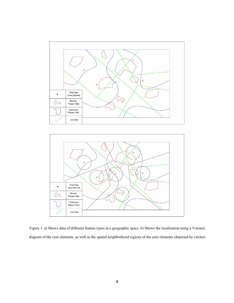
Figure 1 schematically explains the main elements of a problem framework. As it can be seen in Fig. 1-a, in a
general spatial problem, there are different data with different feature types. There are point, line and also polygon

7
data. Based on the concept of spatial autocorrelation summarized in Tobler’s first law of geography (Goodchild
2003), only spatial co-location pattern mining in local regions seems to be meaningful. Spatially restricting the
pattern search not only helps finding meaningful patterns but also significantly reduces the number of co-location
mining searches. Therefore, as can be seen in Fig. 1-b, a localization method — the Voronoi diagram in our case —
can be used to restrict the co-location mining process. Next, however, the method also must have ways of compiling
the different feature type instances in each local region in the mining process. That is, it must integrate the
parameters based on their closeness to the pattern core element. Thus as shown in Fig. 1-b, a neighborhood radius
around the given core elements (depicted by black points) defines circular regions centered around the core
elements, with a given radius to represent the neighborhood relation. Subsequently, the pattern mining algorithm
needs to intersect the different feature type instances with each neighborhood region of core elements to find
interesting co-occurrence patterns.
In addition, it is of paramount importance to mention that finding co-location patterns for a specific time period only
may not be highly beneficial. Therefore, this research intends to develop a pattern mining model which considers
parameters varying in space and time; thus enabling to find spatio-temporal co-occurrence patterns that change over
time as well as tracking their evolution in space and time simultaneously.
8
Figure 1. a) Shows data of different feature types in a geographic space. b) Shows the localization using a Voronoi
diagram of the core elements, as well as the spatial neighborhood regions of the core elements (depicted by circles)
9
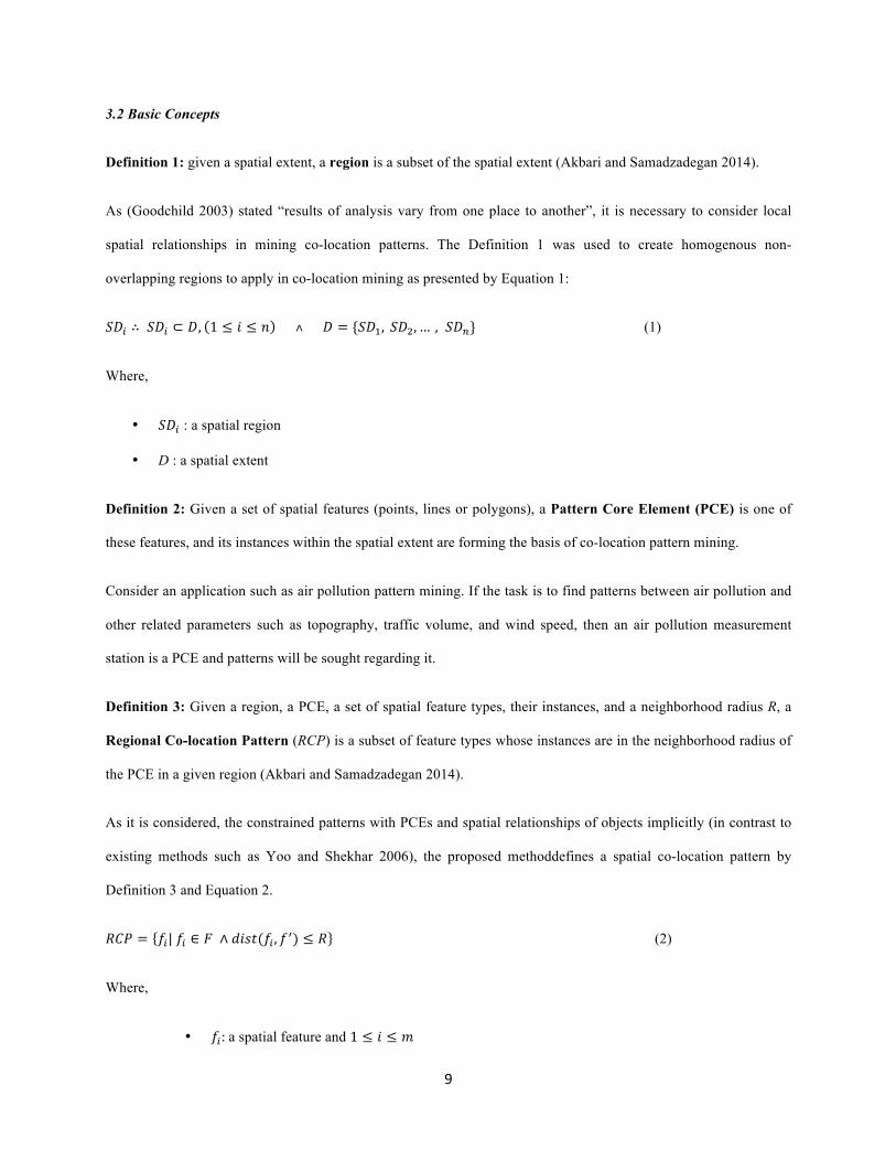
3.2 Basic Concepts
Definition 1: given a spatial extent, a region is a subset of the spatial extent (Akbari and Samadzadegan 2014).
As (Goodchild 2003) stated “results of analysis vary from one place to another”, it is necessary to consider local
spatial relationships in mining co-location patterns. The Definition 1 was used to create homogenous non-
overlapping regions to apply in co-location mining as presented by Equation 1:
𝑆𝐷! ∴ 𝑆𝐷! ⊂ 𝐷, 1 ≤ 𝑖 ≤ 𝑛 ˄ 𝐷 = {𝑆𝐷!, 𝑆𝐷!,… , 𝑆𝐷!} (1)
Where,
• 𝑆𝐷! : a spatial region
• D : a spatial extent
Definition 2: Given a set of spatial features (points, lines or polygons), a Pattern Core Element (PCE) is one of
these features, and its instances within the spatial extent are forming the basis of co-location pattern mining.
Consider an application such as air pollution pattern mining. If the task is to find patterns between air pollution and
other related parameters such as topography, traffic volume, and wind speed, then an air pollution measurement
station is a PCE and patterns will be sought regarding it.
Definition 3: Given a region, a PCE, a set of spatial feature types, their instances, and a neighborhood radius R, a
Regional Co-location Pattern (RCP) is a subset of feature types whose instances are in the neighborhood radius of
the PCE in a given region (Akbari and Samadzadegan 2014).
As it is considered, the constrained patterns with PCEs and spatial relationships of objects implicitly (in contrast to
existing methods such as Yoo and Shekhar 2006), the proposed methoddefines a spatial co-location pattern by
Definition 3 and Equation 2.
𝑅𝐶𝑃 = 𝑓!| 𝑓! ∈ 𝐹 ∧ 𝑑𝑖𝑠𝑡(𝑓! , 𝑓!) ≤ 𝑅 (2)
Where,
• 𝑓!: a spatial feature and 1 ≤ 𝑖 ≤ 𝑚

10
• 𝑓!: PCE
• 𝑑𝑖𝑠𝑡(𝑓! , 𝑓!): Euclidean distance between a spatial feature and a PCE
• 𝑅: Neighborhood radius that is defined based on Euclidean distance around a PCE
• F: set of spatial features
• RCP: Regional Co-location Pattern that is, a subset of problem spatial features which have close
spatial relationships with a PCE.
Definition 4: Given a spatial extent and a set of regions (in our case, Voronoi regions), a PCE is the centroid of
each region (Akbari and Samadzadegan 2014).
The method will mine the co-location patterns in the local spaces, which is called Regions based on Definition 1 and
Definition 3. Due to the challenges of spatial space tessellation mentioned in (Celik et al. 2007), the proposed
partitioning and indexing method for this research is the Voronoi diagram. The Voronoi diagram partitions the plane
into regions, one for each point site, containing all features of the plane which are closer to this site than to any other
(Icking et al. 2003). Therefore, Voronoi diagrams have been formed for PCEs to satisfy Definition 1.
Definition 5: In a co-occurrence pattern mining process, a spatial or temporal prevalent pattern, respectively, is a
pattern whose desirability measure (expressed by the Participation Index or Temporal Prevalence Index; see below)
exceeds a given spatial or temporal threshold, respectively.
Mining spatio-temporal co-occurrence patterns needs to consider the temporal dimension as well as spatial one. As
mentioned before, considering the time dimension in the mining process needs a metric. Due to lack of a suitable
metric, a new temporal metric was proposed that not only can be used in mining prevalent co-occurrence patterns
but also can be used to track the evolution trend of patterns. Subsequently, this criterion labeled as Temporal
Prevalence Index can be defined as follows.
Definition 6: Given a spatio-temporal dataset, the lifetime dimension is the total number of timeslots in the
temporal framework of the problem.
Definition 7: Given a spatio-temporal dataset, and a spatial co-location pattern set, the lifetime size of a pattern
𝐶!! , 2 ≤ 𝑘 ≤ 𝑁𝑜. 𝑜𝑓 𝑓𝑒𝑎𝑡𝑢𝑟𝑒 − 𝑡𝑦𝑝𝑒𝑠 is the total number of timeslots where that pattern is prevalent.

11
Definition 8: Given a size-k co-occurrence pattern set 𝑃𝑆 = 𝐶!!,… ,𝐶!! , (2 ≤ 𝑘 ≤ 𝑁𝑜. 𝑜𝑓 𝑓𝑒𝑎𝑡𝑢𝑟𝑒 − 𝑡𝑦𝑝𝑒𝑠) then,
for pattern 𝐶!! , the Temporal Prevalence Index of 𝐶!! ,𝑇𝑃𝐼 𝑃𝑆,𝐶!! , is the ratio of the lifetime size of pattern 𝐶!! to
the lifetime dimension.
4. RST-CoM: Regional Spatio-Temporal Co-occurrence pattern mining Model
The basic idea of regional co-occurrence pattern mining is to index space and reduce search space in order to
increase efficiency and achieve results based on spatial and temporal concepts. As Celik et al. (2007) mentioned,
common spatial indexing structures are not so applicable for co-location pattern mining. This research applies a
spatial index structure formed by the Voronoi tessellation of the PCEs to efficiently mine regional co-location
patterns having dynamic factors and also dynamic feature type instances. This eliminates the need to examine
objects which are outside the regions of interest (i.e. the Voronoi regions), and the Voronoi index enhances the
computational performance. To consider a realistic application context, this model is extended to handle all feature
types (points, lines, polygons), thus increasing its generality. In addition, in contrast to the existing models for co-
occurrence pattern mining, in this model, a new criterion has been developed that not only can be used to detect
spatio-temporal prevalent co-occurrences, but also can be used to identify trends of evolution of patterns in the
spatio-temporal framework. Therefore, developing RST-CoM to handle the aforementioned abilities can increase the
overall effectiveness of the co-location mining process with respect to time dimension. Algorithm 1 gives the pseudo
code of the RST-CoM algorithm. In the RST-CoM algorithm (cf. pseudo-code in Algorithm 1), line 1 initializes the
parameters. Line 2 invokes the localization of the spatial extent. Lines 3 through 13 represent the core of the
algorithm and are explained in detail below; and line 14 returns the results.
Before describing the actual algorithm, the localization step in line 2 warrants more detail. The PCEs may be of
different feature types (point, line and polygon). If the PCEs are point data then loc_space () creates the Voronoi
regions based on the point PCEs and spatially indexes the features to the Voronoi polygons to localize each feature
to a limited search space. Therefore, when it intends to check different objects in the neighborhood of a PCE, only
the features indexed to that local Voronoi polygon are considered. Alternatively, if the PCEs are line or polygon data
then loc_space () works in a different way. To handle these types of PCEs, we introduce the concept of an MNBR

12
(Minimum Neighborhood Bounding Rectangle). It is defined based on the case in point PCEs. In this case,
loc_space () works as follows: First, using a Euclidean distance R around the feature instances creates a
neighborhood space. Second, a minimum bounding rectangle is generated around the neighborhood space of the
PCE: the MNBR. Third, these MNBRs are used as local regions to index features. Figure 2 depicts the neighborhood
space (dashed line) and the MNBR (solid line) around a polyline and a polygon PCE, respectively. It is noteworthy
that for the purposes of this paper, only the case of point PCEs will be considered.
(a) (b)
Figure 2. a) MNBR for polyline PCE. b) MNBR for polygon PCE
Algorithm 1: RST-CoM
Inputs:
F: a set of distinct spatial feature types,
FI: a set of feature type instances
PCE: a set of pattern core elements
ST: a Spatio-‐Temporal dataset
TF: a time slot framework 𝑡!,… , 𝑡!!!
𝜽𝒔: a spatial prevalence threshold
𝜽𝒕: a temporal prevalence threshold

13
Output:
• Spatio-‐Temporal Co-‐occurrence patterns whose spatial and temporal prevalence indices are greater
than 𝜃! and 𝜃!, respectively.
• Spatio-‐Temporal evolution of Co-‐occurrence patterns in Temporal framework (TF)
Variables:
k: co-‐occurrence size
t: time slots (0, …, n-‐1)
R: spatial neighborhood relationship
Ck: set of candidate size k co-‐locations
Ik: set of instances of size k co-‐locations
SCPk: set of spatially prevalent size k co-‐locations
TPIk: set of temporal prevalence indices of size k co-‐locations
STCk: set of Spatio-‐Temporal size k co-‐occurrences
PMk: set of Spatio-‐Temporal evolution of size k co-‐occurrences
Algorithm
1: Initialization, k=1, Ck= F, STCk=ST
2: loc_space (PCE, F, FI)
3: while (not empty STCk)
4: Ck+1=gen_co-‐occurrence_candidates (Ck, STCk)
5: for each time slot t (0<t<n-‐1)
6: Ik+1 (t) = gen_co-‐occurrence_instances (Ck+1(t), Ik (t), R)
7: SCPk+1 (t) = mine_spatial_prev_co-‐occurrences (Ck+1(t), Ik+1 (t),𝜃!)
8: end for

14
9: TPIk+1 =calc_temporal_prev_indices (SCPk+1 , TF)
10: STCk+1 =mine_ST_prev_co-‐occurrences (SCPk+1 , TPIk+1 , 𝜃!)
11: PMk+1 =mine_ST_evolution_co-‐occurrences (TPIk+1)
12: k=k+1
13: end while
14: return {STC2 , …, STCk+1 , PM2 , …, PMk+1 }
This algorithm has several functions that can be explained as follows. In line 4, the function gen_co-‐
occurrence_candidates() generates size-𝑘 + 1 candidate co-occurrence patterns 𝐶!!! for each time slot based on
all size-𝑘 pattern using an apriori-based method (Agarwal and Srikant 1994). In line 6, the function gen_co-‐
occurrence_instances() works similarly to (Huang et al. 2004) by joining neighbor instances of size-𝑘 spatio-
temporal co-occurrence patterns for each time slot, generating the instances of candidate 𝐶!!!. In line 7, the function
mine_spatial_prev_co-‐occurrences() evaluates the candidates to find those patterns whose spatial prevalence
criteria are greater than a threshold (𝜃!). The spatial prevalence criterion of patterns in this research is the
participation index such as in (Huang et al. 2004), but as mentioned, since it should handle all feature types in the
co-location mining process, it is necessary to extend the existing criteria. Therefore, new participation ratios were
developed according to the following equations 3, 4 and 5. The participation index then is the minimum of the
participation ratios of all feature types in a co-location.
• For point data: 𝑃𝑟 𝐶, 𝑓! = !"(!!)!(!!)
(3)
Where 𝑁𝐼(𝑓!) is the number of 𝑓! feature instances in co-location instance neighborhoods of C and 𝑁 𝑓! is the total
number of 𝑓! feature instances.
• For line data : 𝑃𝑟 𝐶, 𝑓! = !" !!! !!
+ (!!!!!!!!!!⋯ )! !! ×(!!!!!!⋯ )
(4)

15
Where 𝑁𝐼 𝑓! is the number of 𝑓! feature instances that are completely contained in co-location instance
neighborhoods of C and 𝑁 𝑓! is the total number of 𝑓! feature instances. In addition, 𝑙! is the number of line features
of which 𝑤! fraction of length 0 < 𝑤! < 1 falls inside of co-location instance neighborhoods of C.
• For polygon data : 𝑃𝑟 𝐶, 𝑓! = !" !! ! !!
+ (!!!!!!!!!!⋯ )! !! ×(!!!!!!⋯ )
(5)
Where 𝑁𝐼 𝑓! is the number of 𝑓! feature instances that are completely contained in co-location instance
neighborhoods of C and 𝑁 𝑓! is the total number of 𝑓! feature instances. In addition, 𝑙! is the number of polygon
features of which 𝑠! fraction of area 0 < 𝑠! < 1 falls inside of co-location instance neighborhoods of C.
Using a for loop, the algorithm finds size-𝑘 + 1 spatially prevalent co-occurrence patterns for each time slot. In line
9, the function calc_temporal_prev_indices(), based on definitions 6, 7 and 8, calculates size-𝑘 + 1 temporal
prevalence indices of all spatially prevalent patterns size-𝑘 + 1. Then, in line 10, the function mine_ST_prev_co-‐
occurrences() finds all size-𝑘 + 1 spatially prevalent co-occurrences whose temporal prevalence index meets the
temporal threshold (𝜃!). Finally, in line 11, the function mine_ST_evolution_co-‐occurrences() assesses the status
of different size-𝑘 + 1 spatio-temporal co-occurrence patterns and classifies them into 6 states. This categorization
takes place based on the patterns’ temporal prevalence indices (TPI), simultaneously considering spatial prevalence,
since as stated in Definitions 7 and 8, it is introduced based on the spatial participation index (PI):
• If for the temporal framework 𝑇𝐹: 𝑡!, 𝑡!!! → 𝑇𝑃𝐼 𝐶! = 1, then the pattern is SUSTAINED
• If ∃ 𝑡!,𝑚 ∈ 1, 2,… , 𝑛 − 1 so that for 0, 𝑡! → 𝑇𝑃𝐼 𝐶! = 0 and for 𝑡!, 𝑡!!! → 𝑇𝑃𝐼(𝐶!) > 0 then
the pattern is EMERGING
• If ∃ 𝑡!,𝑚 ∈ 1, 2,… , 𝑛 − 1 so that for 0, 𝑡! → 𝑇𝑃𝐼 𝐶! > 0 and for 𝑡!, 𝑡!!! → 𝑇𝑃𝐼 𝐶! = 0 then
the pattern is DISPERSING
• If for the temporal framework 𝑇𝐹: 𝑡!, 𝑡!!! → 0.5 ≤ 𝑇𝑃𝐼 𝐶! < 1, then the pattern is TIME
PREVALENT
• If for the temporal framework 𝑇𝐹: 𝑡!, 𝑡!!! → 0 < 𝑇𝑃𝐼 𝐶! < 0.5, then the pattern is TIME VARIANT
• If for the temporal framework 𝑇𝐹: 𝑡!, 𝑡!!! → 𝑇𝑃𝐼 𝐶! = 0, then there is NO PATTERN

16
5. Experimental Evaluation
In this section, the proposed RST-CoM algorithm was evaluated experimentally with real world data, with the aim
of spatio-temporal co-occurrence pattern mining of air pollution against external drivers and influences, including
road traffic, wind, and topography.
5.1. Datasets
The datasets used include air pollution, meteorology, traffic and topography of part of Tehran (for more information,
see Table 1). The study area can be seen in Fig. 3. The study area consists of regions number 1-8, 21 and 22 of
Tehran city (depicted in different color in Fig. 3). These regions were selected because data were primarily available
for these units and secondly, the data were up-to-date and had enough spatial and temporal overlap. The data span
12 days of different months between 21/03/2011 until 19/03/2012 (a Solar Hijri Year), one day per month.
Table 1. Information about applied data in this research
Parameter Feature
Type
No. of objects No. measurement
stations
Temporal
resolution
Source
Topography (DEM) Polygon 264 --- --- National Cartographic Center
of Iran
Air pollution (Co
pollutant)
Point 108 9 Daily Tehran Air Quality Control
Center
Meteorology (Wind
Speed)
Polygon 36 3 Daily Iran Meteorological
Organization
Road traffic Line 20136 700 Daily Tehran Traffic Control Center

17
Figure 3. Study Area
A selection of feature types in the air pollution pattern mining problem was used as shown in the Table 2. The raw
data were preprocessed to yield the input data for the pattern mining process. Datasets were prepared for each
feature type that included the classification of feature type, time information and spatial position information. As can
be seen in the Table 2, each feature type was classified into 3 different classes to apply them directly to the mining
process (refer to Table 2 for details about the classification). Class breaks were selected after studying the
distribution characteristics of each parameter. For traffic data the classification is based on the original five classes
used by the Tehran Traffic Control Center: Fluent, Disruption in movement, Heavy but moving, heavy, and Very
heavy. The original 5 classes were summarized into 3 classes, Fluent, Semi-Heavy, and Heavy. Similarly for air
pollution, since data were used from the Tehran Air Quality Control Center, their rules for the classification of
pollutants were adopted. This center, on its web site, states the classification for each air pollutant. In this research,
CO data was applied and classified accordingly. For the meteorological parameters, wind data was used, since it is
the meteorological factor that affects air pollution the most (Table 2). The raw data were obtained from the Iran
Meteorological Organization. To classify the wind data based on this organization’s proposal, the Beaufort scale was
used. Finally, for the classification of topography, because Tehran lies on the hill slope of the Alborz Mountains and
its height values differ almost uniformly linear along a cross-section, three meaningful classes were formed after
studying the height variation over Tehran. The detailed class boundaries are shown in Table 2 along with the class
labels that were used in the mining process.

18
Table 2. Detailed classification of case study parameters
Class Subclass Quantity
Domain
Label Class Subclass Quantity
Domain
Label
Traffic
Volume
Fluent Fluent Traffic Tr1
Topography
Down <1300 Tp1
Semi-‐
Heavy
Disruption in
movement/Heavy
but moving traffic
Tr2 Medium 1300-‐1500 Tp2
Heavy Heavy/Very
Heavy traffic Tr3 High >1500 Tp3
Wind
Speed
Low <6 Wn1
CO Pollutant
Low <1 Ap1
Normal 6-‐16 Wn2 Normal 1-‐5 Ap2
High > 16 Wn3 High >5 Ap3
5.2. Implementation Results
As aforementioned, to evaluate the proposed algorithm and also to extract useful patterns of air pollution with the
other affecting parameters in Tehran City, the algorithm was implemented in C#. The implemented interface has 4
tabs: 1. Data View to show and see data and also results; 2. RST-CoM panel, enabling to enter the desired input
values such as Neighborhood Radius, Spatial Prevalence Threshold, Temporal Prevalence Threshold and Temporal
duration. 3. Pattern Visualization panel to visualize the extracted co-occurrence patterns in each time slot, allows to
select a desired time slot and visualize the corresponding spatio-temporal co-occurrence patterns in the spatial
domain (i.e. on a map). 4. Region Statistics panel, which serves to extract some information for different regions and
time slots.
Due to gaps in the time series data, the 4th day of each month over one year was selected, thus yielding totally 12
days. In fact, Persian months were considered and different months were checked for their work days (in Persian
weeks workdays are from Saturday until Wednesday). The 4th day of the month was then selected because it falls
mostly on a workday throughout the year, and also avoids data gaps. The following input values were used.

19
• Neighborhood Radius: 2000 m; this radius was selected based on the average distance between air pollution
measurement stations and spatially meaningful variation of affecting parameters in a neighborhood.
• Spatial Prevalence Threshold: 0.5; this value was selected based on the idea that a pattern is prevalent if its
importance criterion supplies at least for half the participant features.
• Time Prevalence Threshold: 0.6; is selected somewhat higher than 50% such that only the most important
patterns are found.
The pattern mining with RST-CoM applied to the case study leads to interesting results (Fig. 4). In Fig. 4, some
information for each mined time slot has been summarized. For example in Fig. 4, there is a pattern (ap2; tr1) that is
depicted with dark pink color. This pattern can be found in all time slots. This means that there is a pattern between
air pollution type 2 (ap2 in Table 2) and road traffic type 1 (tr1 in Table 2) in all studied time slots. The explanation
for the other patterns in Fig. 4 works accordingly. In other words, Fig. 4 shows extracted patterns in different time
slots in a column chart with different colors, where patterns which have common parts have similar colors.
Figure 4. Pattern distribution in different time slots
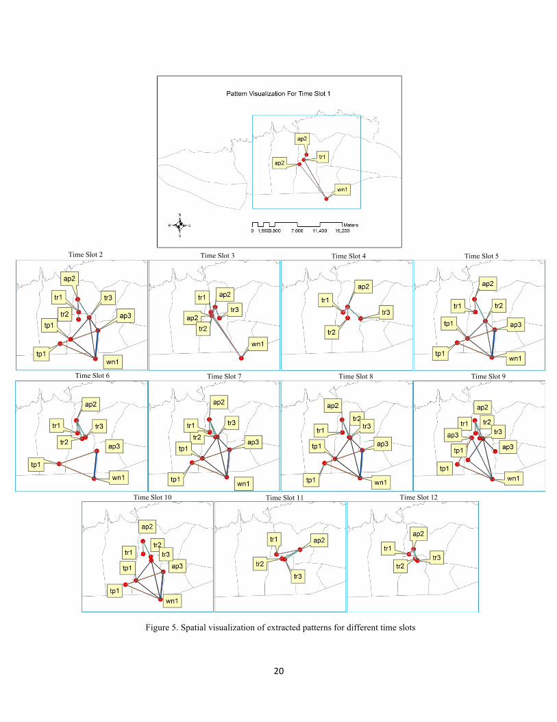
In addition, the spatial visualization of extracted patterns for each time slot is shown in Fig. 5. In the spatial
representation of the extracted patterns, a similar method as introduced by Desmier et al. (2011) for the visualization
of co-location patterns was applied. However, this research has made some extensions to the original method of
Desmier et al. (2011) to handle data of all feature types. In Fig. 5, each illustrated pattern is a surrogate of all similar
prevalent occurring patterns in the spatial extent of the case study. To distinguish each pattern from the others
different colors were used, and to show the importance of a pattern, the line width was varied according to the
associated PI value.
20
Figure 5. Spatial visualization of extracted patterns for different time slots
Time Slot 9 Time Slot 6 Time Slot 7 Time Slot 8
Time Slot 3 Time Slot 4 Time Slot 5 Time Slot 2
Time Slot 10 Time Slot 11 Time Slot 12

21
Of the 60 different assessed candidate patterns that have had 473 compositions in 12 time slots, there were
• 1 Sustained pattern {(ap2; tr1)}
• 5 Time Prevalent patterns {(ap2; tr3), (ap2; tr2), (ap3; tp1), (ap3; wn1), (ap3; tp1; wn1)}
• 11 Time Variant patterns {(ap2;wn1), (ap2;tr1;wn1), (ap3;tr2), (ap3;tr3), (ap3;tr2;tp1), (ap3;tr3;tp1),
(ap2;tr2;wn1), (ap3;tr2;wn1), (ap3;tr3;wn1), (ap3;tr2;tp1;wn1), (ap3;tr3;tp1;wn1)}
• And finally 43 candidates that showed no particular pattern (i.e. exceeded none of the thresholds).
To assess the performance of the proposed model, an efficiency test was conducted on a Notebook with the
following software and hardware configuration:
• Windows 7 Ultimate
• Dual core processor
• 1.86 GHz CPU
• 2 GB DDR2 SDRAM
• 160 GB (5400 rpm) HDD
• 1 MB Cache
The proposed model was evaluated with different neighborhood radiuses. As can be seen in Fig. 6, 5 different
neighborhood radii, 500, 1000, 1500, 2000 and 2500 meters were applied. All other parameters were left unchanged
(number of time slots = 6, spatial prevalence threshold = 0.5, temporal prevalence threshold = 0.6). Fig. 6 then plots
the processor time against different neighborhood radiuses. Two different regression models were then fitted, a
linear model (shown in Fig. 6-a) and a quadratic model (Fig. 6-b). In fact, R2 value in Fig. 6-b shows a better fitting
compared to Fig. 6-a, especially when the radius increases much more than 2500 meters, the fitting will be
quadratic. However in this studied interval, it can be considered as a linear fitting and this research can claim that
the proposed model is of the order of O(n). It is also necessary to mention that radiuses bigger than 3000 m for this
case study were not meaningful since the neighborhood regions start overlapping (the distance between the air
pollution measurement stations is never larger than 5800 m). Furthermore, air pollution neighborhood search beyond
this range is not effective since the maximum variance of pollution has already been reached at this range.

22
a) Linear equation fitting b) Polynomial equation fitting
Figure 6. Variation of processor time against different neighborhood radii As mentioned above, in Regions Statistics Tab of the developed model, three criteria were presented including VDF
(Voronoi Density Function), VGF (Voronoi Gravity Function) and VIF (Voronoi Impact Function). These criteria
can be calculated based on the results of RST-CoM algorithm. They can be defined as follows:
𝑉𝐷𝐹! =!"#$%&'( !"#$%#& !"#$%&" !"#!"#$%& !" !!! !"#"$"% !"#$%&
!"#$% !"#$%& !" !"#$%#& !"#$%&" !"#$%"&'# !" !"#$%#& !"#$%&'"( (5)
𝑉𝐺𝐹! =!"#$%& !" !"!!!"#$%!& !"#$%"&'# !" !!! !"#"$"% !"#$%&
!"#$% !"#$%& !" !"!!"#$%&"' !"#$%"&'# !" !"#$%#& !"#$%&'"( (6)
𝑉𝐼𝐹! =(!"#$!!"# !"!!"#$%&"' !"##$%&' !" !!! !"#"$"% !"#$%&)!
!!!
! (7)
Where in Eq. 7, “m” is the number of prevalent co-location patterns in each region and the weight function is the
Prevalence Threshold (PI). The results of these three criteria for the case study are presented in Figures 7, 8 and 9.
Figure 7. Map of the VDF index for the case study

23
Figure 8. Map of the VGF index for different timeslots
Time Slot 2 Time Slot 3 Time Slot 4 Time Slot 5
Time Slot 6 Time Slot 7 Time Slot 8 Time Slot 9
Time Slot 10 Time Slot 11 Time Slot 12

24
Figure 9. Map of the VIF index for different timeslots
6. Discussion
Using figures 4 and 5, it can be seen that the most prominent and prevalent patterns in the case study are (ap2; tr1),
(ap2; tr3), (ap2; tr2), (ap3; tp1), (ap3; wn1) and (ap3; tp1; wn1). These patterns are classified as Sustained or Time
Prevalent patterns, based on the predefined TPI criteria and classification conditions. The extracted patterns contain
Time Slot 2 Time Slot 3 Time Slot 4 Time Slot 5
Time Slot 6 Time Slot 7 Time Slot 8 Time Slot 9
Time Slot 10 Time Slot 11 Time Slot 12

25
nearly all studied parameters, but it is worth discussing the results in more detail. First, for the air pollution
parameter, there are only occurrences of air pollution classes 2 and 3. Since (Azizi 2011; Kavousi et al. 2013;
Saadatabadi et al. 2012) had mentioned high air pollution as a major problem for Tehran, it had to be expected that
most patterns are co-occurrences having higher levels of air pollution class 2 and 3. It is also evident that with
respect to air pollution as the pattern core element, traffic plays an important role. Since CO was used as air
pollutant in this study and also due to the fact that the most important sources of this pollutant are motor cars, it
makes CO a traffic related pollutant (Azizi 2011; Safavi and Alijani 2006); afterwards, it was also expected that
there are prevalent patterns between air pollution and traffic. The other parameters participating in the above
patterns are topography class 1 (< 1300m) and wind speed class 1 (< 6 knot). As (Safavi and Alijani 2006) explains,
the Alborz mountains located to the north and northeast of Tehran hamper westerly winds and cause air pollutants to
remain in the city. Tehran on the southern slope of the Alborz chain lies in a semi-closed area (Fig. 3). Generally,
the topography of Tehran slopes from north to south, although some height variations can be found in the city as
well. This topographic configuration causes poor wind circulation with low wind speeds, trapping all pollutions in
the city. Authors in (Saadatabadi et al. 2012) conclude that low wind speed is one of the most important
meteorological factors causing high levels of CO concentration. Very clearly, the extracted patterns of the case study
confirm the relationship between high air pollution and low wind speed. Additionally, temperature inversion
occurrences further trap pollutants in the city, especially in central and southern parts of Tehran (Rahimi Ghoroghi
2012; Safavi and Alijani 2006), where the topography class is 1 (i.e. low topography). Therefore, the extracted
pattern of air pollution class 3 (high) and topography class 1 (low) is a valid pattern.
Considering at Figures 4 and 5, two observations can be made regarding the spatial and the temporal distribution of
patterns, respectively. First, most of the patterns concentrate in the central parts of Tehran, that is, regions 2, 3, 6 and
7 shown in Fig. 3. This can be confirmed by the existing rules in Tehran to confront the air pollution problems, in
this case, the Area Traffic Plan that exists for the central parts of Tehran. In addition, (Shad et al. 2009) confirms
that air pollutants concentrate in the central and eastern parts of Tehran. Second, regarding the temporal distribution,
it can be seen that in the first time slots of the series, there are relatively few patterns. Later on, the number of
patterns increases until the 10th time slot and then decreases again.

26
Generally speaking, it shows that most prevalent patterns occur from the beginning of fall until the beginning of
winter. On the other hand, except during the second time slot, low numbers of prevalent patterns occur in the spring,
the beginning of summer and the end of winter. However, perhaps the kinds of patterns that exist in each time slot is
more important than the number of patterns. In Fig. 4, it can easily be understood that most of the patterns in the
period of the beginning of fall to the beginning of winter are those that co-occur with air pollutions of class 3. As
mentioned above, low wind circulation in Tehran is further aggravated by a meteorological situation named
inversion, which occurs most frequently around this time of the year and causes more air pollution (Rahimi
Ghoroghi 2012; Safavi and Alijani 2006). Conversely, in the spring, summer and the end of winter inversions are
less frequent, and thus patterns with air pollution class 3 are rare.
In addition, paying more attention to the extracted patterns shown in Fig. 5, it can be identified that air pollution
class 3 (> 5 ppm CO) has a tendency to occur in the eastern parts of Tehran. As reported in (Rahimi Ghoroghi
2012), the prevalent wind direction in Tehran are westerly winds that move air pollution from the western parts of
Tehran to the eastern parts; however, due to the presence of mountains, they remain blocked in the eastern parts,
increasing the air pollution in that area, as found by (Shad et al. 2009). Repeatedly, this confirms the validity of this
approach.
Considering the extracted patterns from the spatial point of view, it is clear that in time slots having a lower number
of patterns, those patterns are more spatially concentrated compared to in time slots with more patterns. It seems
plausible that whenever there are more patterns, the probability of those patterns covering a wider area is higher.
While the extracted patterns follow this general rule in the spatial distribution, thus confirming the above findings,
some additional information can also be learned. Specifically, as can be seen in Fig. 5, in time slots where only
patterns between air pollution and traffic exist, the line lengths are smaller than in time slots with more parameters
participating in patterns. This confirms the fact that the most important source of air pollution is traffic (Azizi 2011;
Safavi and Alijani 2006), where the geometric centers of air pollution and traffic data lie close to each other. On the
other hand, although low wind speed and topography have a close correlation with air pollution, because of the fact
that those parameters are not the source of air pollution, geometric centers of air pollution and wind speed and
topography, respectively, are not expected to lie as close as is the case for traffic.

27
In Fig. 8, feature density in different regions is showed. As can be seen, central parts of the city show higher
concentrations of features due to the denser traffic network in these parts. Figure 9 depicts the density of prevalent
co-occurrence patterns in each of the study regions. It can be seen that the central parts of the city, especially the
“Ostandari”, “Shahrdari_10” and “Geophysic” regions, respectively, have higher values in most of the VGF maps
which shows that most of the occurring patterns are concentrated in these parts, which is in correspondence with our
previous discussions. Considering Fig. 10 and 9, it is evident that the VIF index does not exhibit the same behavior
as the VGF index. Using Fig. 10, it can be found that in most times, regions that have higher VGF values – that
means more patterns occur in these regions – have lower VIF values, which seems plausible because whenever there
are more patterns indices, the probability of the VIF index to be more balanced is higher.
One of the findings in this research is that although there is a relatively clear trend in pattern change over time, there
are also exceptions from this trend. For example, the patterns of time slot 2 are against the existing trend. This may
be due to some other temporal parameters affecting air pollution that have not been considered. It may also be
caused by the fact that only one day per month was selected, which may cause outliers.
To find an optimal neighborhood radius, as well as the optimal spatial and temporal prevalence thresholds is a
challenge that lies outside the scope of this research but it will be important in order to present the best results for a
decision maker. Clearly, however, these quantities largely depend on the spatio-temporal process under study, and
the parameters that govern this process. In this case, the process studied was air pollution, and the influencing
factors were traffic volume, wind speed and topography. As explained in Section 5, given some knowledge of the
process studied, it is then possible to select input parameter values (neighborhood radius, prevalence thresholds) that
are adjusted to the process.
As there is another way (LUR) to model air pollution and surrounding environmental parameters, but the proposed
method of these research does not need to a good knowledge of air pollution field, extracts rule like air pollution and
affecting parameters, considers patterns evolution during time and finds their trend. Of course the combination of
the LUR modeling and the proposed method of this research can improve the correctness and completeness of this
method.

28
To conclude this discussion, an important contribution of the pattern extraction and visualization model is that
decision makers can spatially and temporally track air pollution patterns in conjunction with the parameters affecting
this process, see the types of relations occurring, their importance, their spatial and temporal distribution, change
over time, and other related factors. Based on the results of this model, urban managers may change management
procedures; for example, after analysis, they may change the Tehran Traffic Area temporally for each month. This
would not only allow defining a realistic area for traffic control but would also reduce the difficulties of people in
limited transportation areas.
7. Conclusion and Future Work
Based on the existing techniques for spatial co-location mining, a new method called RST-CoM for spatio-temporal
co-occurrence pattern mining is developed. The proposed method has several important extensions. First, the pattern
search is localized by indexing the data to a Voronoi tessellation prior to the co-location mining process, thus
reducing the computational cost. Second, another property of the proposed method is that it considers all the feature
types (point, line, and polygon) in co-occurrence pattern mining, which undoubtedly is indispensable for real
applications. Third, the method is developed to explore the temporal evolution of patterns. In contrast to other
studies that consider features as moving objects, this research moved to a higher level and tracked the evolution of
co-occurrence patterns in both space and time, considering the patterns as ‘moving objects’. As a result, it is possible
to classify the trends of co-occurrence patterns into 6 categories: Sustained, Emerging, Dispersing, Time Prevalent,
Time Variant, and No-Pattern. To evaluate the proposed method, it is implemented with the C# programming
language and applied to a real case study: the extraction of air pollution patterns in relation to other influencing
parameters, for the City of Tehran. The results of the experiments suggest that the proposed method may be used for
real applications such as air pollution modeling. Finally, this study introduces new concepts to the domain of spatio-
temporal co-occurrence pattern mining. To find co-occurrence patterns having the same emphasis on the spatial and
temporal dimensions, respectively, is the other goal of this research that has been achieved.
In future studies, we would like to apply or extend our method of spatio-temporal co-occurrence pattern mining to
different application domains such as noise pollution, crime, floods, or car accidents. We also intend to extend our
model for line and polygon as co-occurrence pattern core elements. Furthermore, future research may intend to

29
develop and evaluate more comprehensible approaches of visualizing the extracted co-occurrence patterns in the
spatio-temporal domain. In addition we will try to have a comparison study between co-occurrence pattern mining
and LUR modeling and also we will try to combine them for a more complete model for air pollution modeling.
8. Acknowledgment
We are grateful of the Iran Meteorological Organization, the Tehran Air Quality Control Center, the Tehran Traffic
Control Center and the National Cartographic Center of Iran for providing our casestudy data.
9. References
Agarwal R, Srikant R (1994) Fast algorithms for Mining Association Rules. In: Proceeding of 20th International
Conference on Very Large Data Bases (VLDB). pp: 487-499.
Akbari M, Samadzadegan F (2014) New Regional Co-location Pattern Mining Method Using Fuzzy Definition of
Neighborhood. Adv. in Comput. Sci.: an Intern. J. (ACSIJ), 3(3): 32-37.
Azizi M H (2011) Impact of traffic-related air pollution on public health: a real challenge. Arch. of Iran. Med.,
14(2):139-143.
Beelen R, Hoek G, Vienneau D, Eeftens M, Dimakopoulou K, Pedeli X, ... de Hoogh K (2013) Development of NO
2 and NO x land use regression models for estimating air pollution exposure in 36 study areas in Europe–the
ESCAPE project. Atmos. Env. , 72:10-23. doi: 10.1016/j.atmosenv.2013.02.037
Celik M (2011) Discovering Partial Spatio-Temporal Co-occurrence Patterns. In: Proceeding of 1st International
Conference on Spatial Data Mining and Geographical Knowledge Services. pp: 116-120. Fuzhou, China. doi:
10.1109/ICSDM.2011.5969016.

30
Celik M, Azginoglu N, Terzi R (2012) Mining Periodic spatio-temporal co-occurrence patterns: a summary of
results. In: International Symposium on Innovations in Intelligent Systems and Applications (INISTA).
pp:411-415. Trabzon, Turkey. doi: 10.1109/INISTA.2012.6247044.
Celik M, Kang J M, Shekhar S (2007) Zonal Co-location Pattern Discovery with Dynamic Parameters. In:
Proceeding of Seventh IEEE International Conference on Data Mining. pp: 433-438. Omaha, NE. doi:
10.1109/ICDM.2007.102.
Celik M, Shekhar S, Rogers J P, Shine J A (2008) Mixed-drove Spatiotemporal Co-occurrence Pattern Mining.
IEEE Trans. on Knowl. and Data Eng., 20(10):1322-1335. doi: 10.1109/TKDE.2008.97 .
Champendal A, Kanevski M, Huguenot P E (2014) Air Pollution Mapping Using Nonlinear Land Use Regression
Models. In Computational Science and Its Applications–ICCSA 2014, pp: 682-690. Springer International
Publishing. doi: 10.1007/978-3-319-09150-1_50
Desmier E, Flouvat F, Gay D, Selmaoui-Folcher N (2011) A clustering-based visualization of colocation patterns.
In: Proceedings of the 15th Symposium on International Database Engineering & Applications. pp: 70-78.
ACM. doi:10.1145/2076623.2076633.
Ding W, Jiamthapthaksinl R, Parmar R, Jiang D, Stepinski T F, Eick C F (2008) Towards Region Discovery in
Spatial Datasets. In: Proceeding of Pacific-Asia Conference on Knowledge Discovery and Data Mining
(PAKDD). pp: 88-99. Osaka, Japan. doi: 10.1007/978-3-540-68125-0_10.
Goodchild M F (2003) The fundamental laws of GIScience. Invited talk at University Consortium for Geographic
Information Science, University of California, Santa Barbara.
Gudmundsson J, Kreveld M V (2006) Computing Longest Duration Flocks in Trajectory Data. In: Proceeding of the
ACM International Symposium on Geographic Information Systems. pp: 35-42. Virginia, USA.
doi:10.1145/1183471.1183479.
Huang Y, Shekhar S, Xiong H (2004) Discovering co-location patterns from spatial datasets: A general approach.
IEEE Trans. on Knowl. and Data Eng. 16(12):1472-1485.

31
Huang Y, Zhang L, Zhang P (2008) A Framework for Mining Sequential Patterns from Spatio-Temporal Event
Datasets. IEEE Trans. on Knowl. and Data Eng. 20(4): 433–448. doi: 10.1109/TKDE.2007.190712.
Icking C, Klein R, Kollner P, Ma L (2003) Java Applets for the Dynamic Visualization of Voronoi Diagrams.
Comput. Sci. in Perspect., Lect. Notes in Comput. Sci. 2598:191-205. doi: 10.1007/3-540-36477-3_14.
Kanaroglou P S, Adams M D, De Luca P F, Corr D, Sohel N (2013) Estimation of sulfur dioxide air pollution
concentrations with a spatial autoregressive model. Atmos. Env., 79:421-427.
doi:10.1016/j.atmosenv.2013.07.014
Kavousi A, Sefidkar R, Alavimajd H, Rashidi Y, Khonbi Z A (2013) Spatial analysis of CO and PM10 pollutants in
Tehran city. J. of Paramed. Sci. (JPS), 4(3): 41-50. ISSN: 2008-4978.
Manikandan G, Srinivasan S (2012a) Mining of Spatial Co-location Pattern Implementation by FP Growth. Indian J.
of Comput. Sci. and Eng. (IJCSE), 3(2): 344-348, ISSN: 0976-5166.
Manikandan G, Srinivasan S (2012b) Mining Spatially Co-Located Objects from Vehicle Moving Data. Eur. J. of
Sci. Res., 68(3): 352-366, ISSN: 1450-216X.
Miller H. J., & Han, J. (2009). Geographic Data Mining and Knowledge Discovery. 2nd edition, London: CRC Press,
published, 486pp.
Mohan P, Shekhar S, Shine J A, Rogers J P (2010) Cascading Spatiotemporal Pattern Discovery: A Summary of
Results. In: Proceeding of the SIAM International Conference on Data Mining (SDM): pp: 327-338.
Priya G, Jaisankar N, Venkatesan M (2011) Mining Co-location Patterns from Spatial Data using Rulebased
Approach. Int. J. of Glob. Res. in Comput. Sci., 2(7): 58-61.
Qian F, He Q, He J (2009a) Mining Spread Patterns of Spatio-temporal Co-occurrences over Zones. In: Proceedings
of the international conference on computational science and applications. pp: 686–701. doi: 10.1007/978-3-
642-02457-3_57.

32
Qian F, Yin L, He Q, He J (2009b) Mining spatio-temporal co-location patterns with weighted sliding window. In:
IEEE International Conference on Intelligent Computing and Intelligent Systems ICIS 2009. pp: 181-185.
doi: 10.1109/ICICISYS.2009.5358192.
Rahimi Ghoroghi N (2012) Evaluation of geographical factors on Tehran air pollution and its relation with
temperature inversion. In: First Conference of air and noise pollution management. Tehran, Iran.
http://www.civilica.com/Paper-CANPM01-CANPM01_039.html. (In Persian)
Saadatabadi A R, Mohammadian L, Vazifeh A (2012) Controls on air pollution over a semi-enclosed basin, Tehran:
A synoptic climatological approach. Iran. J. of Sci. & Technol. (IJST), 4: 501-510.
Safavi S Y, Alijani B (2006) Evaluation of Geographical parameters in Tehran air pollution. Geogr. Res. J., 58: 99-
112. (In Persian)
Shad R, Mesgari M S, Shad A (2009) Predicting air pollution using fuzzy genetic linear membership kriging in
GIS. Comput., Environ. and Urban Syst., 33(6):472-481.
Shekhar S, Huang Y, Xiong H (2001) Discovering Spatial Co-location Patterns: A Summary of Results. In:
Proceeding of 7th International Symposium on Spatial and Temporal Databases (SSTD). Redondo Beach,
CA, USA. doi: 10.1007/3-540-47724-1_13.
Wan Y, Zhou J (2008) KNFCOM-T: a k-nearest features-based co-location pattern mining algorithm for large
spatial data sets by using T-trees. Int. J. of Bus. Intell. and Data Min., 3(4): 375-389. doi:
10.150/IJBIDM.2008.022735.
Xiao X, Xie X, Luo Q, Ma W (2008) Density based co-location pattern discovery. In: Proceeding of ACM
SIGSPATIAL International Conference on Advances in Geographic Information Systems (ACM-GIS).
Irvine, CA, USA. doi: 10.1145/1463434.1463471.
Xiong H, Shekhar S, Huang Y, Kumar V, Ma X, Yoo J S (2004) A framework for discovering co-location patterns
in data sets with extended spatial objects. In: Proceeding of the 2004 SIAM international conference on data
mining (SDM’04). Lake Buena Vista, FL. pp: 78-89.

33
Yoo J S, Bow M (2011) Mining Top-k Closed Co-location Patterns. In: Proceeding of IEEE International
Conference on Spatial Data Mining and Geographical Knowledge Services (ICSDM). Fuzhou. pp: 100-105.
doi: 10.1109/ICSDM.2011.5969013.
Yoo J S, Shekhar S (2005) A Partial Join Approach for Mining Co-location Patterns. In: Proceeding of ACM
SIGSPATIAL International conference on Advances in Geographic Information Systems (ACM-GIS). pp:
241-249. doi:10.1145/1032222.1032258.
Yoo J S, Shekhar S (2006) A Join-less Approach for mining Spatial Co-location Patterns. IEEE Trans. on Knowl.
and Data Eng., 18(10):1323-1337. doi: 10.1109/ICDM.2005.8.