a generic framework for design evolution: from …
TRANSCRIPT
A GENERIC FRAMEWORK FOR DESIGN EVOLUTION: FROM FUNCTION-TO-FORM MAPPING TO SYNTHESIS OF TOLERANCES
By
Nilmani Pramanik
B.E.(Mech), (Hons), Jadavpur University, India M.E., Birla Institute of Technology and Science, India
DISSERTATION
Submitted in partial fulfillment of the requirements for the degree of Doctor of Philosophy in Mechanical and Aerospace Engineering
in the graduate School of Syracuse University.
June 2003
Approved __________________ Professor Utpal Roy
Date __________________

Copyright 2003 Nilmani Pramanik
All rights Reserved

The Graduate School Syracuse University
We, the members of the Oral Examination Committee, hereby approve the Thesis/dissertation of
Nilmani Pramanik
Candidate’s Name
Whose oral examination was held on
May 30, 2003
Date
Dr. Alan J. Levy
Examiner (Please type) (Please sign)
Dr. Chilukuri Mohan
Examiner (Please type) (Please sign)
Dr. Frederick Easton
Examiner (Please type) (Please sign)
Dr. Young B. Moon
Examiner (Please type) (Please sign)
Dr. Utpal Roy
Thesis/dissertation Advisor (Please type) (Please sign)
Dr. Eric M. Lui
Chair, Oral Examination Committee (Please sign) (Please type)

Abstract
Design of a new product (artifact) begins with a set of user specifications which are
functional requirements (FRs) that the artifact must satisfy. Initially, the set of FRs is
almost always incomplete because complete knowledge about the product is not known at
the conceptual design stage. In this work, two complementary schemes are presented: a
design synthesis scheme for conceptual design and a tolerance synthesis scheme for
manufactured parts. In the first phase, a function-to-form mapping process is presented to
arrive at a conceptual design that satisfies the FRs. This process is carried out in stages of
design evolution and at each stage the product specification (PS) is transformed using
FRs as constraints and variation of internal parameters of artifacts as navigator for the
mapping process. In the second phase, which starts after the nominal dimensions of the
parts of an artifact have been computed (using domain-specific design rules), a method
for synthesis of tolerances for manufactured parts is presented as an optimization process
for minimizing manufacturing cost subject to constraints of assemblability and functional
requirements. A generic deviation-based formulation has been used to represent the
variations of features and the entities in the tolerance synthesis process have been
modeled in UML using object-oriented representation. A new deviation-based model for
manufacturing cost has been introduced. The optimization scheme is used to find a set of
optimal deviation parameters, which are then transformed into standard tolerance
specifications as per ASME Y14.5M (1994) tolerancing schemes using a deviation-to-
tolerance mapping system. The tolerance synthesis scheme is implemented to serve as a
tool that could be linked with standard CAD packages to give the designer a mechanism
for iterative solution for product development and tolerance synthesis.

v
Table of Contents Abstract … i
Table of Contents … v
List of Illustrative Materials … viii
Acknowledgement … x
Nomenclature … xi
Chapter 1. Introduction … 1
1.1 Introduction and Motivation … 1
1.2 Objectives of the Thesis … 4
1.3 Organization of the Thesis … 5
Chapter 2. Review of Related Research … 7
2.1 Design Synthesis … 7
2.2 Tolerance Synthesis … 10
Chapter 3. Representation of Artifact and Associated Classes … 13
3.1 Product Specifications … 14
3.2 Artifact Representation … 16
3.2.1 Artifact Classification … 17
3.2.2 Generic Definition of Artifact … 18
3.2.3 Representation of Internal Parameters of Artifacts … 19
3.3 Representation of Functions … 22
3.4 Representation of Behaviors … 24
3.5 Artifact Library … 25
3.6 Tolerance Representation … 26
Chapter 4. Design Synthesis: Function-to-Form Mapping … 29
4.1 Transformations of Product Specification (PS) … 32
4.2 Attribute Transformation … 32
4.3 Constraint Transformation … 33

vi
4.4 Variation of Internal Parameters of Artifacts … 35
4.5 Design Synthesis Process … 39
4.6 Observations on the Design Synthesis Process … 46
4.7 An Example of Design Synthesis … 47
Chapter 5. Tolerance Synthesis Scheme … 56
5.1 Representation of Deviations of Features of a Part … 57
5.1.1 Local Coordinate System on a Feature … 59
5.1.2 Invariants of a Feature and Reduction of DOF … 60
5.2 Tolerance Synthesis (TS) Scheme … 62
5.3 Deviation of Features and Assembly of Mating Parts … 63
5.3.1 Gap as a Control Element between Mating Features … 66
5.3.2 Shifting the Point of Interest … 66
5.4 Generation of Constraints … 67
5.4.1 Constraints Related to Functional Requirements … 68
5.4.2 Constraints Related to Assemblability of Parts … 69
5.5 Formulation of Cost Functions … 73
5.5.1 Cost of Manufacturing … 73
5.5.2 Deviation-based Model for Cost of Manufacturing … 75
5.6 Optimization Process … 79
5.7 Mapping Deviation Parameters to Tolerance Specification … 80
5.7.1 Deviation-to-Tolerance Mapping Criteria … 82
5.7.2 Mapping Relations for a Planar Feature … 84
5.7.2.1 Rectangular Planar Feature … 85
5.7.2.2 Circular Planar Feature … 86
Chapter 6. Implementation and Case Studies … 88
6.1 Details of the Implementation … 88
6.2 Example Tolerance Synthesis of a 3-block Artifact … 92
6.3 Example Tolerance Synthesis of a Planetary Gearbox … 100

vii
Chapter 7. Conclusion … 109
7.1 Contribution … 109
7.2 Future Work … 110
Appendices
Appendix – 1 Class diagrams for various classes … 114
Appendix – 2 Examples of artifact representation … 118
Appendix – 3 Artifact Library … 126
Appendix – 4 Interval Arithmetic … 129
Appendix - 5 Transformation of Torsors … 131
Appendix - 6 Example of Generation of Assemblability Constraints … 136
Appendix – 7 Mapping of Deviation Parameters to Tolerance Parameters … 141
Appendix – 8 Implementation: Listing of major modules … 150
Appendix – 9 Tolerance Synthesis Example –1: A three-block system … 170
Bibliography … 174
Vita (biographical data) … 183
viii
List of Illustrative Materials
Figure 4.5 Schematic diagram for transforming input functions to outputs … 40
Figure 4.7-1. Design Synthesis - some intermediate stages … 52
Figure 4.7-2. Typical solutions from the Design Synthesis example … 53
Figure 5.1.1. Local coordinate system on a feature … 60
Figure 5.1.2. Deviation parameters of a circular-planar feature … 61
Figure 5.3-1. A spur gear sub-assembly …. 64
Figure 5.3-2. Mating details of the gear sub-assembly … 64
Figure 5.3-3. Assembly graph of the gear sub-assembly … 65
Figure 5.3.2. Points of interest on features … 67
Figure 5.4.2. Traversing Paths/Loops in an assembly graph … 71
Figure 5.5.2-1. Cost as function of deviation parameters … 78
Figure 5.5.2-2. Cost contour lines and the bounds … 78
Figure 5.7.2.1. Rectangular planar feature … 85
Figure 5.7.2.2. Circular planar feature with size tolerance … 86
Figure 6.2-1. A 3-Block Artifact … 93
Figure 6.2-2. 3-Block Artifact - Part #1- Nominal shape with LCS … 94
Figure 6.2-3. 3-Block Artifact – Artifact tree … 95
Figure 6.2-4. 3-Block Artifact - Feature to feature connectivity … 96
Figure 6.2-5. 3-Block Artifact – Assembly graph … 97
Figure 6.2-6. Sample cost of Manufacturing Function … 97
Figure 6.2-7. Deviations imposed on nominal shape … 98
Table 6.2-1. Optimal deviation parameters … 98
Table 6.2-2. Tolerance values mapped from optimal deviation parameters … 99
Figure 6.2-8. Computed tolerance parameters for Part #1 … 99
Figure 6.3-1. A Planetary Gearbox … 100
Figure 6.3-2. Exploded view of the gearbox … 101
Figure 6.3-3. Gearbox modeled as a 5-part system … 101
Figure 6.3-4. Mating of output housing with output shaft and ring gear … 102

ix
Figure 6.3-5. Assembly graph (connectivity diagram) of the gearbox … 102
Figure 6.3-6 Circular planar feature with tolerance parameters TU and TL … 106
Table 6.3-1 Tolerance zones/values for cylindrical features … 107
Table 6.3-2 Tolerance zones/values for circular planar features … 108
Figure A1.1 Artifact class diagram … 114
Figure A1.2 Function Class … 115
Figure A1.3 Behavior Class … 115
Figure A1.4 Material Data Class … 116
Figure A1.5 Feature Class … 116
Figure A1.6 Tolerance Class … 117
Figure A5-1 Interacting torsors at mating surfaces … 132
Figure A5-2. Torsor transformation - shifting axes … 133
Figure A6-1 Example artifact with three blocks … 136
Figure A6-2 – 3-Block artifact with feature numbers and LCS … 137
Figure A7.1-1 Cylindrical feature with tolerance modified to MMC … 142
Figure A7.1-2 Cylindrical feature with LCS … 142
Figure A7.2-1 Spherical feature with LCS … 144
Figure A7.2-2 Spherical feature with tolerance specification … 145
Figure A7.4-1 Size tolerance for a planar feature … 148
Figure A7.4-2 Deviation space for size tolerance of a planar feature … 149

x
Acknowledgement
I would like to express my sincere gratitude to my academic advisor Prof. U. Roy for his
guidance, support, and encouragement throughout my program of study and research
work. It has been a pleasure to work with him.
I would take this opportunity to thank Dr. Alan J. Levy, Dr. C. K. Mohan, Dr. Y. B.
Moon, Dr. Eric M. Lui, and Dr. Fred Easton for consenting to serve as members of my
dissertation committee.
I would also like to thank my friends and colleagues at the Knowledge Based
Engineering Laboratory, specifically, Mr. Haoyu Wang and Mr. Saujesh Patel, for their
support and many meaningful discussions/interactions.
Finally, I would like to express my sincere appreciation and thanks to my wife
Shyamalsovana and daughter Ananya for their infinite patience, continued support, and
love without which it would have been impossible for me to complete my research work.

xi
Nomenclature Unless otherwise specified in the context, following nomenclature will be used throughout the thesis. Also, mathematical variables are used in italics and non-scalar quantities like vectors, matrices, torsors, classes, sets, etc., are used in bold typeface.
Symbol Meaning
::= defined as | alternatives (choices) <> attribute | parameter | entity | token delimiter [ ] optional item delimiter … use as subscript to indicate one or more repetitions ∀ for all ∃ there exists ∪, ∩ union, intersection of sets ∅ NULL set ⊃, ⊇ super set of ⊂, ⊆ subset of (belongs to) ⊄ not a subset of ∈ element of ∉ not an element of : such that =, EQ equal to (assignment operator) ≡ equivalent to ≈ approximately equal to !, NOT not &, AND and NE, !=, ≠ not equal to LT, < less than LE, <= less than or equal to GT, > greater than GE, >= greater than or equal to == equality comparator => implies ∑ summation over a range ∏ product over a range R 1-d real space R+ 1-d real positive half-space R- 1-d real negative half-space Rn
n-d real space ∞ infinity (a large positive number) -∞ negative infinity (a large negative number)

1
Everything is vague to a degree you do not realize till you have tried to make it precise. -- Bertrand Russell
Chapter 1
Introduction
1.1 Introduction and Motivation
Design as a process to create new artifacts1 to meet the challenges of the society is a
complex task. It is motivated by many different factors including economic, socio-
political and creative urges. In this thesis design and manufacturing of artifacts to meet
technological challenges are discussed. With the advancement of computers and
computing techniques, the focus of design has shifted from manual design computations
to automated design using powerful computational aids like artificial intelligent tools,
rule based expert systems, and use of domain-specific knowledge bases. However, the
process of product development requires interaction and exchange of ideas between
experts from various design domains. Since there is high degree of specialization in each
domain, to facilitate effective collaboration between these design experts, a common
framework for representing the entire design process is required so that all personnel
involved in the process could interact and exchange data, knowledge and ideas in a
consistent manner. Design of a new artifact could be grouped into three distinct phases,
namely, 1) conceptual design, 2) detail design for sizing the components/parts, and 3)
manufacturing and assembly (including inspection and quality control). The first phase
(conceptual design) involves conceiving physical shapes/structures from the functional
1 The term artifact has been used in this thesis in a generic sense to represent assembly and subassembly of parts, parts, components, and other design objects/products.

2
requirements (FRs). The mechanism to transform a set of FRs into suitable form, called
function-to-form (F2F) mapping, is not well established and oftentimes the process is not
unique due to possibility of one-to-many mappings and variations. However, these one-
to-many mappings give some creative space for the designer to explore alternative
solutions as will be seen in the design synthesis process in chapter 3. Even though there
have been many domain-specific approaches for F2F, there is no generic universal
system for F2F mapping. Whitney (1992) attributed this to “the lack of basic engineering
knowledge that can link form and function, the lack of a mature concept of a product data
model, and/or the lack of a mature concept of the product design process.” Most of the
function-to-form mapping systems (as discussed in chapter 2) are very domain-specific
and lookup domain-specific rules. In this work a generalized framework has been
presented that could automate the design synthesis process for F2F mapping.
After a successful F2F mapping phase, the conceptual design is still not very ‘concrete’
in shape – only the basic functional requirements could be satisfied at this stage and
detailed design calculations are required to establish physical size of the components that
would deliver the desired outputs. Since this part is purely domain specific, an attempt to
generalize the process of detail design would be futile. For example, procedures for
designing the shape and size of gas turbine blades could be entirely different to those for
designing the teeth of a bevel gear. Attempt to generalize all such diverse design steps in
a single framework would defeat the purpose and computational overheads could go up.
Also, domain-specific detail design procedures are well established and there are national
and international standards and codes (like ANSI, DIN, ISO, JIS, etc.) that regulate and
guide the detail design process. In this work this phase of detail design has not been

3
treated. However, the generic artifact class presented here is flexible enough for adding
domain-dependent design procedures.
The third phase of design starts after nominal sizes and dimensions of each
part/component of the artifact has been computed in the previous stage of detailed design.
In this stage a new challenge emerges as the parts have to be manufactured and no part
could be manufactured with the nominal size and shapes (theoretical/exact sizes). Some
deviation or distortion from the ideal shape must be allowed and even then, the artifact
should satisfy the original functional requirements (as far as feasible), and the parts must
be assemblable (geometric compatibility). A third challenge comes from economic
considerations: the overall total cost associated with manufacturing, assembling,
inspection, quality control and other life-cycle costs should be minimized to make the
artifact economically viable/competitive. In this thesis, a generic tolerance synthesis
scheme has been established that could be used for synthesis of geometric tolerances for
manufactured parts and the synthesis process can take care of assemblability constraints,
functional requirements and minimizes suitable cost functions.
Since the two major tasks (conceptual design and tolerance synthesis) are part of the
same design process, a need for generalized treatment is necessary. With the development
of object-oriented design and development methodology as a powerful tool for
representation of entities in hierarchical class structures, the possibilities of representing
complex process and entities in a systematic manner is possible. Particularly, defining a
class as an abstract entity and subsequent instantiation of the same class to add specific
4
details (forms) of the abstract entities could be effectively used to represent design
entities that are either partially defined or vaguely defined at the conceptual design stage
and evolves gradually as the design proceeds towards detailed design with more concrete
shape/structure. An integrated approach to represent the artifact as an artifact class could
be used to drive a design synthesis process in a generic manner to explore new horizons
in design evolution in a multitude of design domains. The possibility of extending the
artifact class to represent and guide detail design processes like manufacturability,
assemblability, quality management and tolerance design could lead to a paradigm shift
in integrated design. This thesis presents a framework to integrate the design synthesis
process starting from the conceptual design stage and extending to the details design
stage.
1.2 Objectives of the thesis
The main objectives of the thesis are:
i) Development of a generic artifact class to represent a product: Artifact class
is defined along with all other major classes (function, behavior, structural, etc.)
that are associated with an artifact and an artifact library is established for use in
the design synthesis.
ii) Development of a design synthesis process: A design synthesis (DS) is
established that uses the class structures defined above to drive a design evolution
based on a product specification (PS) and functional requirement (FR).

5
iii) Development of a tolerance representation scheme: A tolerance class is
defined to represent standard industrial tolerancing systems: size tolerance,
position tolerance, orientation tolerance, and form tolerance.
iv) Development of a generic deviation-based tolerance synthesis scheme: A
tolerance synthesis scheme is developed to establish tolerance parameters based
on a minimization of cost of manufacturing function subject to constraints of
assemblability of parts (geometric compatibility) and constraints of functional
requirements.
v) Development of a deviation-base cost of manufacturing formulation: A
deviation-based cost of manufacturing formulation has been developed that could
be used for cost of manufacturing function in the cost optimization process.
vi) Development of a system of mapping deviation parameters of features to
tolerance parameters as per ANSI tolerancing standards: The deviation based
optimization scheme is used to find a set of deviation parameters for the features,
which are then mapped to tolerance zones conforming to industrial standard
tolerancing schemes as per ANSI Y14.5.
1.3 Organization of the Thesis
Research in the areas of product design and tolerance synthesis is reviewed in chapter
two. All class structures that are required for the design synthesis and tolerance synthesis
process are defined with appropriate examples in chapter three. These include: Product
specification (PS), Artifact representation, Functional representation, Behavior
representation, Constraints representation, and Tolerance representation.

6
The design synthesis process is presented in chapter four. Various transformation rules
used to drive the design synthesis process are also defined and a primitive artifact library
(ARTL) is established. These chapter deals with: attribute transformation, constraint
management, variation of internal parameters of artifacts and design synthesis process.
Chapter five deals with representation of deviation of features and the tolerance synthesis
scheme. These include: representation of deviation of features, generation of
assemblability constraints, generation of constraints for functional requirements, cost of
manufacturing formulation, formulation of the tolerance synthesis scheme and deviation-
to-tolerance mapping.
Computer implementation of the design synthesis and tolerance synthesis schemes is
discussed in chapter six. Details of example case studies have been presented in this
chapter to elaborate the steps involved in the synthesis process. Computational aspects
like complexity, efficiency, convergence, and possibility of linking the methods with
existing commercial CAD software like SolidWorks, Pro/E, AutoCAD, etc. have been
discussed.
In the final chapter (chapter seven) contributions in the fields of design evolution and
tolerance synthesis are discussed and areas for future research work are earmarked.

7
Believe those who are seeking truth. Doubt those who find it. --Andre Gide
Chapter 2
Review of Related Research
2.1 Design Synthesis
In the past, the research efforts involving part functions were mainly focused in four
major areas: i) development of standard vocabularies for part functions; ii) development
of ontologies for functions; iii) conceptual design with abstract part functions; and iv)
design with spatial relationships.
In order to fill up the gap between the concept design (from a given set of functional
descriptions) and actual geometry-based CAD, researchers were first trying to create a
computer-aided design system that would help designers explore non-geometric concepts
and to create rough realizations. Pahl and Beitz (1984) suggested a procedure for
deriving the overall functions of a design from the given design problem statements; and
then decomposing and recomposing individual sub-functions to a hierarchical functional
structure that could be mapped to appropriate physical elements. Though the method
provides useful suggestions regarding function decomposition process, it however, does
not relate the functions to design geometry.
Kota (1990) viewed mechanical designs as being synthesized from conceptual building
blocks that perform specific kinematic functions. The motion synthesis approach
provides a method for recognizing a given behavior in terms of known primitive

8
behaviors. This is one of the first formalized ways of viewing design as the synthesis of
kinematic processes; however, the approach is limited to a fixed set of primitives. Hundal
and Byrne (1991) and Iyengar, Lee and Kota (1994) have developed Function Based
Design (FBD) Systems in which a configuration of parts is determined on the basis of the
user specified functions (input and output quantities of a part). The FBD systems are
only useful in the conceptual design stage and do not take into account the interaction
between the parts at the geometric level. Schmekel (1989) has presented a formal
language which consists of a symbolic functional model to describe the functions of a
product. The functions of the product are decomposed into relationships, which are
mapped onto functions of standard components. It, however, only deals with standard
machine elements. Kannapan and Marshek (1991) have developed a design reasoning
system for developing design concepts based on functional and geometric requirements
of mechanical systems built using different machine elements.
Rinderle with Hoover (1989) and Finger (1989) have described a procedure in which
design specifications are transformed into an actual physical artifact using the bond graph
technique. This bond graph technique has also been adopted by a number of other
researchers because of its flexibility of modeling hybrid systems, such as electro-
hydraulic electro-mechanical, etc. using the same symbols and mathematics throughout.
However, bond graphs cannot be used for representing detailed part functions as they
abstract a number of functional details and do not account for spatial relationships.
Ulrich and Seering (1989) have used bond graph techniques to transform a graph of
design requirements into functionally independent physical components. Their technique

9
is useful in the domain of conceptual design but cannot be used for detailed part design.
Bracewell, et al (1995) has extended the bond graph based conceptual design scheme by
coupling it with a parametric 3D geometric modeler. Gui and Mantyla (1994) have
studied a behavior modeling technique for components in assemblies. They have
developed a set of behavioral specifications, which can be used to specify the inter-
relationships between sub-components and have focused on the issue of representing
these relationships.
There are also several reported research programs [Baxter (1994), Henson (1994), Wong
(1993), Sriram (1991, 1992), Gorti (1996), Krause (1993), Pahl (1984), Reddy (1994),
Finger (1992), Finger (1990), Cutkosky (1993), Roy (1999a, 1999b), Szykman (1999),
Sharp (1998)] on the development of system frameworks for product modeling where
function, behavior and product modeling have been discussed. The MOSES research
program jointly undertaken by the Loughborough Institute of Technology and University
of Leeds [Baxter (1994), Henson (1994)] have explicitly focused on the development of
product models for representing different types of part attributes such as part function,
manufacturing details and assembly. Sriram (1991) and Wong (1993) have developed
the DICE (Distributed and Integrated environment for CAE) system with a view of
addressing the coordination and communication problem in the product design process.
Sriram's earlier work on the development of a flexible knowledge-based framework
(CONGEN, CONcept GENerator ) provides methods for generating concepts during the
initial stages of the design [Sriram (1991), Gorti (1996)]. CONGEN consists of a layered
knowledge base (including domain independent knowledge sources like, synthesizer,

10
geometric modeler, constraint manager, evaluator, etc.), a context mechanism, and a user-
friendly interface. The architecture of CONGEN could be enhanced to address the life-
cycle issues of a product and to consider the entire design/manufacturing processes of a
product that is still in the preliminary stages of design. Szykman, Racz, and Sriram
(1999) have proposed a generic scheme for representation of functions and associated
flows. The scheme provides a mechanism for mapping from function domain to physical
domain through references to artifacts. It supports both decomposition of functions into
sub-functions and functions with multiple inputs and output flows.
However, what is missing from the previous works is an integrated approach to the
modeling, representation and decomposition of part functions into an useful format which
can be used for conceptual design as well as for detailed design including addressing
issues involving tolerance synthesis, manufacturability and assemblability. In this work,
a generic design evolution method has been introduced that could be applied to a variety
of design domains.
2.2 Tolerance Synthesis
Tolerance synthesis (TS) essentially means determination of tolerance type and tolerance
value or tolerance zone as per industrial standards (in this thesis tolerances are used as
defined in ASME Y14.5 standard) for each component of an artifact. Tolerancing
concepts as used to be the practice in the industry (mainly plus-minus type size
tolerances) went through major changes with the introduction of geometric tolerancing
that are no more confined to the absolute size of a feature – its interaction and role in the
entire artifact (positional tolerance, orientation tolerance) became more and more

11
important. Many researchers have proposed different schemes for tolerance synthesis
based on various tolerance representation schemes and some form of cost minimization
schemes. Most of these deal with size tolerances, some deal with statistical tolerances and
some with analysis of geometric tolerances.
Requicha (1983) introduced a concept of variational class for representation of tolerances
in geometric modeling and proposed to treat tolerances as attributes of the features. Roy
and Liu (1988a, 1988b) proposed a hybrid CSG/B-Rep scheme for representation of
tolerances and a frame-based was used to store the attributes. Tsai (1993) presented a
frame based semantic network for tolerance representation. Jayraman and Srinivasan
(1989a, 1989b) proposed a virtual boundary method for representing tolerances.
Greenwood and Chase (1987) used a cost-tolerance model to solve the tolerance
optimization problem. Turner and Wonzy (1988) used variational geometry principles to
represent tolerances.
Although all the above methods are suitable for domain-specific usage, none of them
could be considered generic method for representation and treatment of three-
dimensional variation of features in a systematic manner. Also, these methods do not
provide a consistent mechanism for mapping the geometric tolerances to standard codes
(ANSI Y14.5) for industrial usage. Apart from individual researches that produced many
interesting results on tolerance representation and synthesis results, ANSI adopted
standards for geometric tolerances for industrial practice. Of particular interest is the
ASME Y14.5M, 1994 that defines the basis of mathematical representation and

12
interpretation of different geometric tolerances. Although, these tolerancing standards are
effective in industrial applications, it’s very difficult to treat them on a generic basis for
automated tolerancing computations.
Ballot and Bourdet (1998, 2002) used the small deviation torsor (SDT) scheme for
representing the deviation of geometric features in a very elegant way. They used the
torsor transformation rules for generating the geometric variations of parts in a product.
In their work, they have introduced schemes for generating the geometric compatibility
conditions and variation of features for different geometric configurations. Although the
procedure is very good in representing the small variations of geometric shapes, they
have not explicitly shown the possibility of using the SDT scheme for carrying out
tolerance synthesis work. Specifically, how the deviation parameters could be used to
represent cost of manufacturing and other cost factors associated with a part and how the
deviation parameters could be mapped from the deviation space to the tolerance space for
industrial applications.
In this work, the SDT scheme has been adopted for representation of deviation of features
and a generic scheme has been proposed for synthesis of tolerances that can be used for
modeling a wide variety of artifacts. The deviation parameters have been used to define a
new cost of manufacturing formulation for the tolerance synthesis process (minimizing of
cost of manufacturing). Also, in order to make the tolerance synthesis scheme suitable for
industrial tolerancing as per ASME Y14.5M, suitable deviation to tolerance mapping
schemes have been introduced and possibility of linking these schemes with standard
CAD packages has been discussed.

13
To define a thing is to substitute the definition for the thing itself. -- Georges Braque
Chapter 3
Representation of Artifact and Associated Classes
In this chapter all the entities that would be required for the design synthesis and
tolerance synthesis work are defined using an object-oriented approach. For some classes
a BNF-like1 definition is used to capture the essence of the class. Here the strict
formalities of BNF are not used; instead a BNF-like structure is used to represent the
essential features of each entity using following notation:
Symbol Meaning ::= defined as < > delimiter for tokens / identifiers / parameters [...] optional components … used as subscript to denote one or more repetition of a component
for example, {x}… would mean {x} or {x}{x} or {x}{x}{x} … | delimiter for alternate choices, for example {red | blue | green} { } and ( ) grouping of entities
Actual classes diagrams have been developed in UML2 using standard UML notations
for association, aggregation and generalization links between classes. Some of the major
class diagrams are presented in Appendix-1. For some of the classes self-referential
aggregation is used to define dependency on itself in a recursive manner, for example, the
artifact class uses other artifacts (primitive and/or composite parts) to represent a
composite artifact.
1 BNF = Backus Normal Form or Backus-Naur Form is used for defining syntactic entities for production rules and grammars. 2 Unified Modeling Language. The class diagrams have been generated using argoUML- an OpenSource UML-based case tool developed in Java. (http://argouml.tigris.org)
14
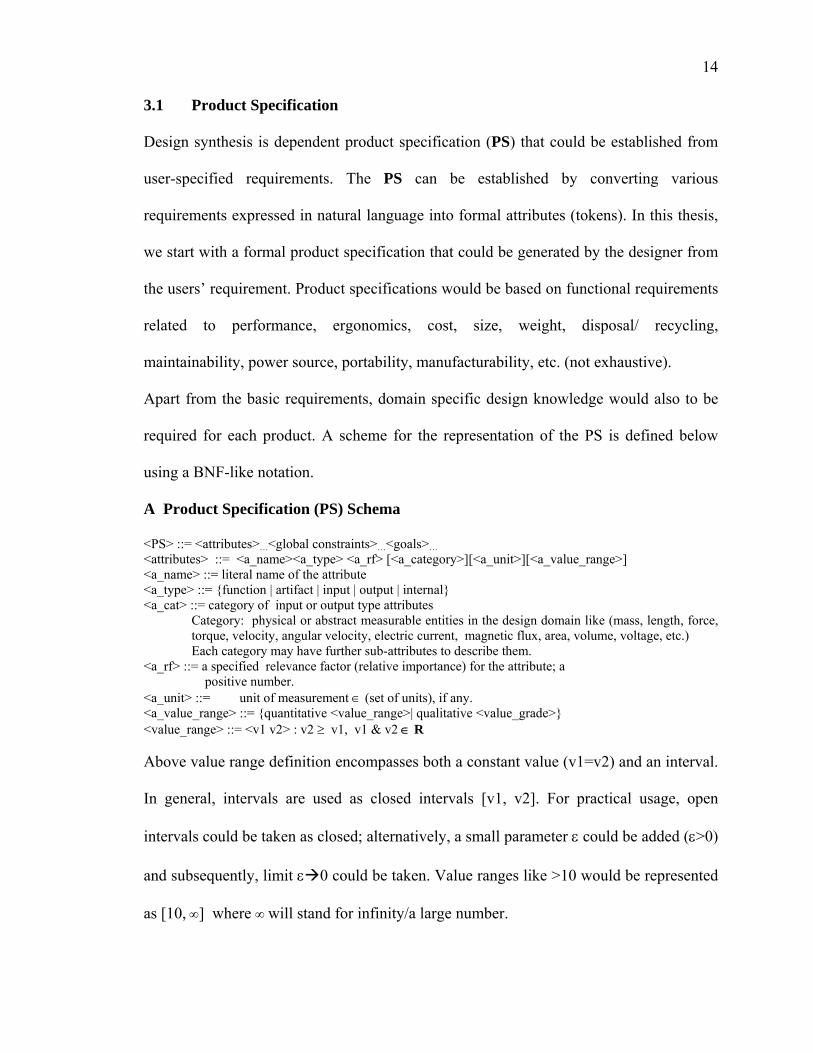
3.1 Product Specification
Design synthesis is dependent product specification (PS) that could be established from
user-specified requirements. The PS can be established by converting various
requirements expressed in natural language into formal attributes (tokens). In this thesis,
we start with a formal product specification that could be generated by the designer from
the users’ requirement. Product specifications would be based on functional requirements
related to performance, ergonomics, cost, size, weight, disposal/ recycling,
maintainability, power source, portability, manufacturability, etc. (not exhaustive).
Apart from the basic requirements, domain specific design knowledge would also to be
required for each product. A scheme for the representation of the PS is defined below
using a BNF-like notation.
A Product Specification (PS) Schema
<PS> ::= <attributes>…<global constraints>…<goals>… <attributes> ::= <a_name><a_type> <a_rf> [<a_category>][<a_unit>][<a_value_range>] <a_name> ::= literal name of the attribute <a_type> ::= {function | artifact | input | output | internal} <a_cat> ::= category of input or output type attributes
Category: physical or abstract measurable entities in the design domain like (mass, length, force, torque, velocity, angular velocity, electric current, magnetic flux, area, volume, voltage, etc.) Each category may have further sub-attributes to describe them.
<a_rf> ::= a specified relevance factor (relative importance) for the attribute; a positive number.
<a_unit> ::= unit of measurement ∈ (set of units), if any. <a_value_range> ::= {quantitative <value_range>| qualitative <value_grade>} <value_range> ::= <v1 v2> : v2 ≥ v1, v1 & v2 ∈ R Above value range definition encompasses both a constant value (v1=v2) and an interval.
In general, intervals are used as closed intervals [v1, v2]. For practical usage, open
intervals could be taken as closed; alternatively, a small parameter ε could be added (ε>0)
and subsequently, limit ε 0 could be taken. Value ranges like >10 would be represented
as [10, ∞] where ∞ will stand for infinity/a large number.

15
<value_grade> ::= qualitative grade ∈ (VH HI MO LO VL) with, for example, possible grade membership values: {VH/1 HI/0.75 MO/0.5 LO/0.25 VL/0.0) <global constraints> ::= a set of relations amongst the attributes Constraints have been considered in three categories: relational, causal and spatial <relational> ::= function(<attribute_name>[,<attribute_name>]…) EQ <value_range>
For example: in a rotary motion transformation, a global constraint requiring a speed
reduction of [5,6] could be represented by: PS.ωI.value/PS.ωO.value EQ (5,6), where ωI
is input and ωO is output rotary speed. If the values were specified as a range, the
arithmetic operators for working with intervals would be required. This has been
discussed in chapter 4 (section 4.3) where constraint transformations have been detailed.
<causal> ::= <attribute> {influences | depends_on} <attribute>[,<attribute>]… Causal constraints indicate dependency of one attribute on other attributes but the exact functional relation may not be known. These types of dependencies are useful for studying the qualitative behavior of an artifact.
<spatial> ::= <attribute> <spacial_relationship> [<attribute>] [a_value]
This constraint is applicable for attributes that are of category ‘artifact’. This would represent spatial (form) relationship between attributes having shape / size / orientation related properties.
<spatial_relationship> ::= <orientation><position><connection> <orientation> ::= <direction cosine of attribute1 w.r.t. that of attribute2> . Some examples of common orientations are: horizontal, vertical, perpendicular_to,
parallel_to, distance_from, etc. and some examples of spatial constraints (for a chair)
could be:
(‘arm’ parallel_to ‘seat’ ) (‘backrest’ perpendicular_to ‘seat’) (‘seat’ horizontal) (‘seat’ distance_from ‘base’ 2ft) …. <position> ::= co-ordinate of center of attribute1 w.r.t. center of attribute2 <connection> ::= <connection_type><contact_details> <connection_type> ::= <point2point | point2surface | surface2surface | others> <contact_details> ::= set of points, surface, and common DOF of connection. <global goals> ::= <objective function>[< constraints>] <objective function> ::= global optimality evaluation functions. As for example: minimize total_weight() or minimize cost(), etc.

16
It may be emphasized here that evaluation of global goals may not be feasible
immediately after a conceptual feasible solution has been arrived at. After a feasible
solution has been found that satisfy the input / output requirements and the constraints,
the solution has to be converted into a physical solution by a rough-cut detailed design
(sizing) to establish nominal dimensions of the parts (artifacts) and then the global goals
could be evaluated.
As an example, using above definition, a product specification for “an artifact that can
drill holes using standard drill bit” could be represented as an object:
product handheld_drill ( (fun to_drill ( (attr hole) (requires (art drillbit)) (requires (fun rotary_motion (art drillbit))) (requires (fun axial_movement (art drillbit))) (requires (fun to_hold (art drillbit))) ) (attr hole output 1.0 (attr (diameter length))) (attr diam output 1.0 mm (0,10)) (attr leng output 1.0 mm (0,100)) (attr input power 1.0 watt (goal minimize)) (attr weight goal 0.5 kg (goal minimize)) (attr volume goal 0.5 mm3 (goal minimize)) (attr cost goal 0.4 dollar (goal minimize)) (attr handheld goal ? ?) )
3.2 Artifact Representation
The term artifact is used here synonymously with physical object, device, component and
assembly (or sub-assembly) of components. In the object-oriented approach, all entities
like artifact, function, device, etc, are defined as classes. An artifact will have its
functional details, structural details and behavior model along with links to other artifacts
/ functions. The modeling of an artifact and its components for use in conceptual design
as well as in detailed design stage, including synthesis and analysis of geometric
tolerances, requires a high-level description which can be represented by a set of

17
attributes. This attribute/sub-attribute set forms a symbolic representation of the artifact
that can be manipulated by the design synthesis process as described in chapter 4.
3.2.1 Artifact Classification
Artifacts could be categorized according to their usage, generic shapes and functional groups. This would facilitate efficient retrieval of artifacts from the artifact library. As for example, following list could be used for parts having similar mechanical functionality (Thornton’s list, Thornton (1994).
Group Artifacts Containers Cover, Housing, Plate, Duct, Pipe Controllers Valve, Gauge, Knob, Pointer, Nozzle Fasteners Clip, Bolt, Nut, Strap, Rivet Coupling, Pin Load Bearers Bracket, Brace, Bearing, Web, Pillar, Rod, Spring Locators Joint, Spacer, Pivot, Pad, Key, Pin Power Transmitters Chain, Cable, Shaft, Pulley, Cam, Gear, Piston Seals Gasket, O-ring, Sleeve
The artifact representation model consists of three basic parts: a functional representation,
a structural (form) representation, and a behavioral representation. The form of an artifact
is expressed in terms of its constituent components and sub-components, and the
interactions between them. The form of each artifact representation consists of
information about
• component/sub-component structure of the artifact • typical shape with the critical dimension outlined • rules for selecting and sizing the artifact • alternate shapes (and/or overall dimensions) • list of additional features and services which would be required to make the
artifact work in a real-life environment, • possible modes/situations in which the artifact might fail; and • material properties.
Components in a composite artifact (assembly) are also of type artifact and the assembly
contains references to these components. Components can be of two different varieties:
18
primitive or composite. Composite components are those whose internal substructure is
represented explicitly by a set of more detailed, lower-level sub-components, whereas
primitive components are simple.
The Artifact model contains artifact-specific information that not only helps in design
synthesis but also in studying its behavior in an assembly. Along with the key artifact
characteristics and component/sub-component structural description, the data model must
contain information on artifact tolerances and its kinematic variations. A detailed
definition of the artifact is presented below:
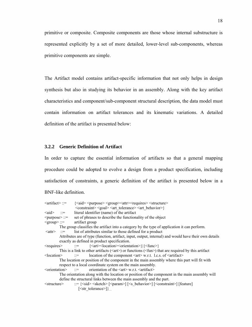
3.2.2 Generic Definition of Artifact
In order to capture the essential information of artifacts so that a general mapping
procedure could be adopted to evolve a design from a product specification, including
satisfaction of constraints, a generic definition of the artifact is presented below in a
BNF-like definition.
<artifact> ::= {<aid> <purpose> <group><attr><requires> <structure> <constraint> <goal> <art_tolerance> <art_behavior>}
<aid> ::= literal identifier (name) of the artifact <purpose> ::= set of phrases to describe the functionality of the object <group> ::= artifact group
The group classifies the artifact into a category by the type of application it can perform. <attr> ::= list of attributes similar to those defined for a product
Attributes are of type (function, artifact, input, output, internal) and would have their own details exactly as defined in product specification.
<requires> ::= {<art><location><orientation>}|{<func>} This is a link to other artifacts (<art>) or functions (<fun>) that are required by this artifact
<location> ::= location of the component <art> w.r.t. l.c.s. of <artifact> The location or position of the component in the main assembly where this part will fit with respect to a local coordinate system on the main assembly.
<orientation> ::= orientation of the <art> w.r.t. <artifact> The orientation along with the location or position of the component in the main assembly will define the structural links between the main assembly and the part.
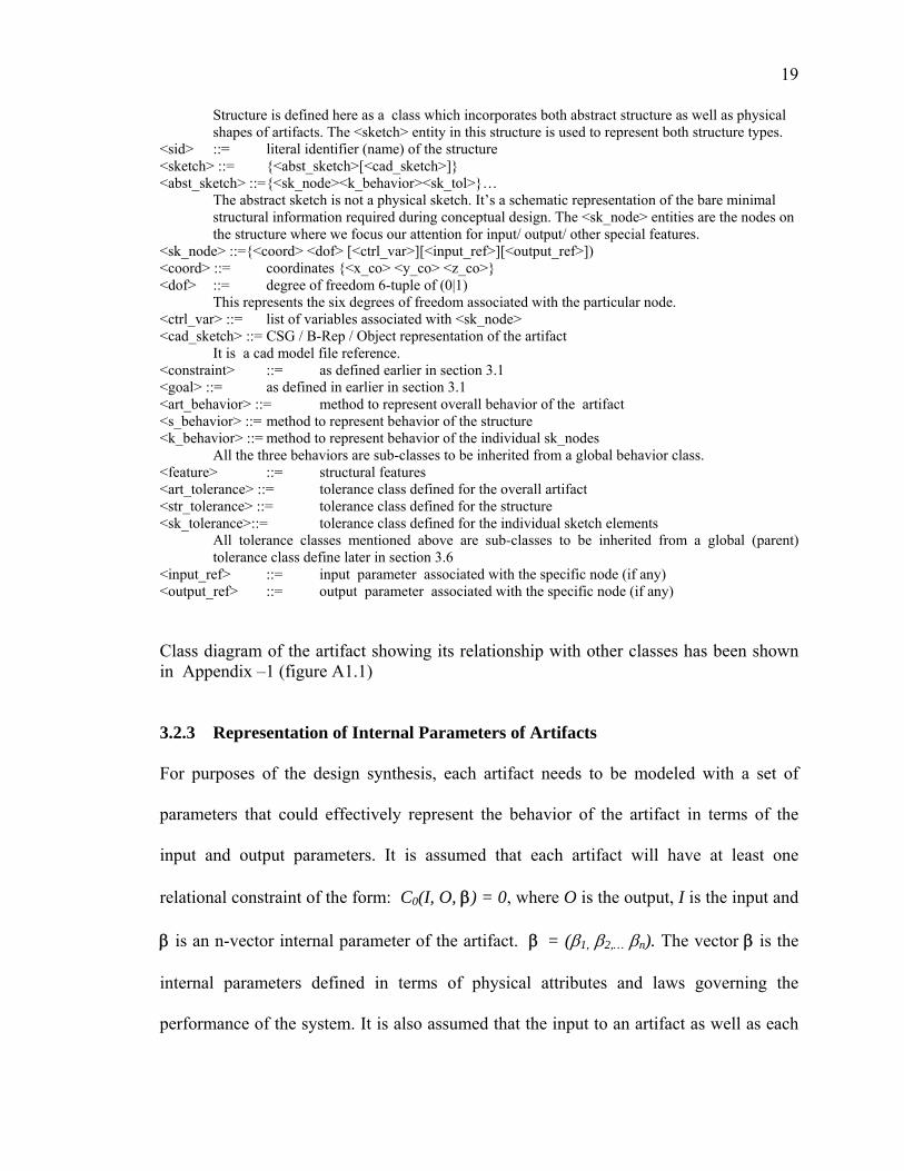
<structure> ::= {<sid> <sketch> [<param>] [<s_behavior>] [<constraint>] [feature] [<str_tolerance>]}…
19
Structure is defined here as a class which incorporates both abstract structure as well as physical shapes of artifacts. The <sketch> entity in this structure is used to represent both structure types.
<sid> ::= literal identifier (name) of the structure <sketch> ::= {<abst_sketch>[<cad_sketch>]} <abst_sketch> ::= {<sk_node><k_behavior><sk_tol>}…
The abstract sketch is not a physical sketch. It’s a schematic representation of the bare minimal structural information required during conceptual design. The <sk_node> entities are the nodes on the structure where we focus our attention for input/ output/ other special features.
<sk_node> ::={<coord> <dof> [<ctrl_var>][<input_ref>][<output_ref>]) <coord> ::= coordinates {<x_co> <y_co> <z_co>} <dof> ::= degree of freedom 6-tuple of (0|1)
This represents the six degrees of freedom associated with the particular node. <ctrl_var> ::= list of variables associated with <sk_node> <cad_sketch> ::= CSG / B-Rep / Object representation of the artifact
It is a cad model file reference. <constraint> ::= as defined earlier in section 3.1 <goal> ::= as defined in earlier in section 3.1 <art_behavior> ::= method to represent overall behavior of the artifact <s_behavior> ::= method to represent behavior of the structure <k_behavior> ::= method to represent behavior of the individual sk_nodes
All the three behaviors are sub-classes to be inherited from a global behavior class. <feature> ::= structural features <art_tolerance> ::= tolerance class defined for the overall artifact <str_tolerance> ::= tolerance class defined for the structure <sk_tolerance>::= tolerance class defined for the individual sketch elements
All tolerance classes mentioned above are sub-classes to be inherited from a global (parent) tolerance class define later in section 3.6
<input_ref> ::= input parameter associated with the specific node (if any) <output_ref> ::= output parameter associated with the specific node (if any)
Class diagram of the artifact showing its relationship with other classes has been shown in Appendix –1 (figure A1.1)
3.2.3 Representation of Internal Parameters of Artifacts
For purposes of the design synthesis, each artifact needs to be modeled with a set of
parameters that could effectively represent the behavior of the artifact in terms of the
input and output parameters. It is assumed that each artifact will have at least one
relational constraint of the form: C0(I, O, β) = 0, where O is the output, I is the input and
β is an n-vector internal parameter of the artifact. β = (β1, β2,… βn). The vector β is the
internal parameters defined in terms of physical attributes and laws governing the
performance of the system. It is also assumed that the input to an artifact as well as each

20
component of the parameter β will have a known feasible range of values. These limits
are the physical ranges within which the artifact can operate. Each component of β can be
expressed in parametric form as: βk = βk_Low + (βk_High - βk_Low) * θk : θk ∈ (0,1) ,
k∈(1,n), where βk_Low is the lower limit and βk_High is the upper limit of value of βk .
Above relational constraint, C0(I,O,β) = 0, could be solved* for O, giving O = f (I, β).
This representation shows the main causal link between the input and the output of the
artifact.
As for example, a gearbox to reduce/increase the speed would have an internal parameter
µ which is the ratio of the number of teeth of the two gears and the main constraint is: C0
(Ni , N0 , µ) ≡ N0 - µ * Ni = 0 where Ni is the input speed, N0 is the output speed and µ is
the speed ratio. µ could have a range of, say, [0.25, 4], indicating that the gear box could
be used for reduction of speed of up to 1/4th as well as for increasing the input speed by 4
times. Depending on specific requirements dictated by the solution, suitable value of β
(here µ) will be selected.
Apart from the main causal link, C0, that links the input and the output, there could also
be several other constraints associated with an artifact which has the general form of:
Cj(I, O, β) <rel_opr> <val>, j >0
where <rel_opr> ∈ (LT LE EQ GE GT NE) is the relational operator and <val> ∈ R,
is a numeric value. In some cases, these relations would be converted to the standard
equality form Cj(I, O, β) = 0, by introducing additional auxiliary variables for the cases
* In general, all constraint equations may not be solvable to express the output as an explicit function of the inputs. In such cases, approximate numeric solutions could be attempted by linearizing the equations around an operating point using small perturbations.

21
where the <rel_opr> is not “EQ”. As for example, Cj(I, O, β) ≡ β1 GE 12.00 would be
converted to: Cj(I,O,β) ≡ β1 – t – 12.00 = 0, where t ∈ R+ is an auxiliary variable.
Along with all the information as described in the definition (section 3.2.2), each
component of an artifact needs to be modeled as being composed of a single material.
Materials are represented as members of material class.
The artifact definition should also have an attribute linked to a database of manufacturing
“know-how” (which has not been included in the present artifact definition). It should
also contain information on material-specific process capabilities and characteristics.
Two examples to represent an artifact using these definitions have been shown in
Appendix-2. There are two artifacts: the first one is a primitive (a spur gear) and the
second one is a compound artifact (a gearbox consisting of six primitive artifacts: two
spur gears, two shafts and two keys). While both the representations use the same artifact
definition given above, the second artifact uses the first artifact through the “requires”
parameter.
The representation for the spur gear (primitive artifact) begins with a list of physical
properties/attributes like material, diameters, thickness, etc. (we can add/modify as many
parameters as would be necessary to define the artifact). The 'input' and 'output' are
then listed. The 'requires, ‘constraints’, 'form / structure' and 'behavior' parameters then
follow. In this case, there was no constraint specified. The ‘behavior’ has been defined as
a set of state-space variables associated with the artifact.
22
For the gearbox (compound artifact), the representation follows a similar logic, however,
in this case, the ‘requires’ clause uses the spur gear primitive (defined earlier) along with
shaft and key elements. Also, in this case a constraint has been added as a relationship
between the output and the input. This forms the main constraint C0 defined earlier in this
section. The behavior also reflects the outcome of the combined elements.
3.3 Representation of Functions
In the early phase of design, most of the design decisions taken are concerned with the
desired characteristics and the overall functions of the assembly. By “Function” is meant
an abstract formulation (or definition) of a task that is independent of any particular
solution. In this phase, the abstract functional specification of an artifact is transformed
into a physical description. In the later phases of design, the physical decisions that are
made in the earlier phases, are elaborated to ensure that they satisfy the specified
functional requirements and life cycle evaluation criteria. In order to manipulate the
“function” information, a “functional data model” (that describes the functional
information throughout the design cycle) is needed so that appropriate reasoning modules
can interrogate and extract functional information during the decision-making processes
(as the geometric reasoning modules query data from the “product data model” (CAD
model) during the shape design process).
Depending on the design phase, different types of functions exist at different levels of
abstraction. In conceptual design phase, functions are usually independent of working
principle, whereas in later design phases, when the functions are detailed, they become

23
more and more dependent on the working principle that has been selected. Therefore, we
need to adopt such a formal function representational scheme that will be helpful when
modeling the overall function of the assembly in the conceptual design stage, and also be
useful to model smaller and smaller sub-assembly, particularly as the component and
feature levels are approached. The representation should also have unambiguous
semantics in order to perform analysis on (i.e. to manipulate) the functional description.
In this work, an attempt has been made to give a definition of a function, which captures
some of the basic features at abstract level, as well as detailed design level. Functions
defined here are also having a mechanism to incorporate functional equivalence classes
associated with a function. This means that a function will have references to other
functions that can collectively be considered equivalent to the function. The collective
equivalence could be of a combination of functions connected by ‘AND’ and ‘OR’ or
combinations thereof. Domain specific knowledge could be used to define such
equivalence classes. This will be a fundamental feature for functional decomposition
during the design process.
As for example:
function (‘rotary_motion to rotary_motion’) could be expressed as equivalent to: function(‘rotary_motion to linear_motion’) AND function(‘linear_motion to rotary_motion’)
A BNF-like definition for the function is given below:
<function> ::= {<fid> <input> [<art>…] <output> <constraint><eqv> <goal>} <fid> ::= literal identifier (name) of the function <input> ::= set of <input_par> <art> ::= artifact through which functional requirements are achieved. <output> ::= set of <output_par> <constraint> ::= set of <relationship> defined over the inputs, outputs and internal attributes of the function <eqv> ::= functional equivalence as discussed above <goal> ::= {<optimality_measure_function>[<constraint>…]}… <input_par> ::= {<iid><category><weight>[<unit>][<value_range>]}…

24
<iid> ::= literal identifier (name) of the input <output_par> ::= {<oid><Category><Weight>[<unit>][<value_range>)… <oid> ::=literal identifier (name) of the output <weight> ::= relative weigh of this parameter for this function <unit> ::= unit of measurement ∈ (set of units) <value_range> ::= as defined in section 3.1
A class diagram of the function class is shown in Appendix-1 (figure A1.2)
3.4 Representation of Behavior
The functional model as discussed in the earlier section is useful for conceptual design
where the design concept is evolved on the basis of the specified abstract functions.
However, the functional model is not sufficient to synthesize assembly/components
behavior. This is because of the fact that functional models do not adequately capture the
interactions of forces and kinematic motions between the part geometry. For instance, the
fit condition between a shaft and a bore cannot be expressed by a spatial relationship
since it does not provide functional design details such as contact pressure, contact force,
rotational torque, rotational speed, etc. at the shaft-bore interface. In order to synthesize
product/assembly behavior and geometric tolerances, full behavioral models of the
involved components in the assembly (including both the structural and kinematic
behavioral models) are required.
Behavior of a function is defined to be the set of values of parameters (which are related
causally) of the function either at a specified time or a series over a period of time
[Chandrasekaran (1996)]. Behavior of a function is context sensitive and as such,
behavior comes into play only in the context of a form. A function defined as an abstract
object often can be achieved through different forms / devices and the function will have

25
different behavior under each separate form / device context. A general behavior class is
defined using BNF-like structure as below:
<behavior> ::= {<state_var> <causal_link><value_ref>} <causal_link> ::= {[<depends_on>] [<affects_var>]} <depends_on> ::= set of variables that influences this variable
Represents input, if this set is null. <affects_var> ::= set of variables that are influenced by this variable
Represents output, if this set is null. <value_ref> ::= {<tabulated>|<procedural>} <tabulated> ::= set of (time, value), at discrete time ∈ R+, value ∈ R <procedural> ::=procedure to return value of the variable at specified time.
The procedure could be in a closed form parametric function of time x = x(t) or an implicit functional representation f(x, t) = 0 that can be solved for x, given t > 0 or some procedural representation which has no closed form but x could be computed, given t.
As for example:
(flow_rate (depends_on (area_of_flow) (pressure)) (affects_var pressure_drop) (procedural (if flow_is_turbulent() then flow_rate(t) := f1(t) else flow_rate := f2(t) )
) Figure A1.3 in Appendix 1 gives a class diagram of the behavior class.
3.5 Artifact Library
The proposed design synthesis process (as detailed in chapter 4) is based on searching
artifact library containing artifacts that could meet specific functional requirements; in
other words, an artifact library (ARTL) is needed that contains artifacts with known
inputs, outputs and a set of variable internal parameters. This artifact library could be
thought of as a knowledge base for searching artifacts that meet specified input/output
patterns in specified design domains.

26
As mentioned in section 3.3, functions could have their equivalent classes and so also
could artifacts – the functionalities of an artifact could be met by combination of two or
more artifacts. The artifact library could contain this knowledge for ease of searching. In
order to illustrate the steps for the design evolution, a sample artifact library has been
developed (Appendix – 3) and the same has been used in the design synthesis example
shown in Chapter 4.
3.6 Tolerance representation
All five categories of tolerances specification, size, form, orientation, run out and location
tolerances (as per ASME Standard Y14.5M-1994), have to be represented in the tolerance
data structures. Tolerance specification involves the specification of a datum reference
frame (DRF) and the relationship among five kinds of tolerance shape elements: vertex,
edge, surface, axis and median plane [Roy (1998)]. Whenever a tolerance specification
requires a datum system to establish the position and orientation of features with respect
to other features, a datum reference frame is provided. It may be three-plane coordinate
system, axes, or an ordered set of features. Size tolerances provide limits for the size
(linear and angular) of a feature, the extent within which variations of geometric form as
well as size are permissible. The size data structure contains a record of the nominal
value and its maximum and minimum variations. Form tolerances (straightness, flatness,
roundness and cylindricity) are used on individual features (single surface, edge, axis or
median plane) and its data structures needs the description of the form tolerance type and
the specific tolerance value. Angularity, parallelism and perpendicularity are included in
orientation tolerance. The data record of the orientation tolerance includes types of
27
orientation tolerance, tolerance value, MMC (material) condition and a pointer to the
DRF record. Tolerances of location state the permissible variation in the specified
location of a feature in relation to some other feature(s) or datum(s). Its data structure
contains location tolerance type, type of tolerance shape element, tolerance value, MMC
conditions, and a pointer to the DRF record.
The incorporation of tolerance models within the artifacts solid model is fundamentally
based on applying tolerance as the design constraints to the solid objects. These
constraints are driven by the features parameters of the solid object as well as by its
geometry. Constraints are specified to both unevaluated (CSG) and evaluated (B-Rep)
forms of the solid model. The constraint descriptions are independent of the “set
operator” description of the solid model and they are specified and attached to the
tangible and intangible topographical entities only, apart from the CSG and B-Rep data
structure.
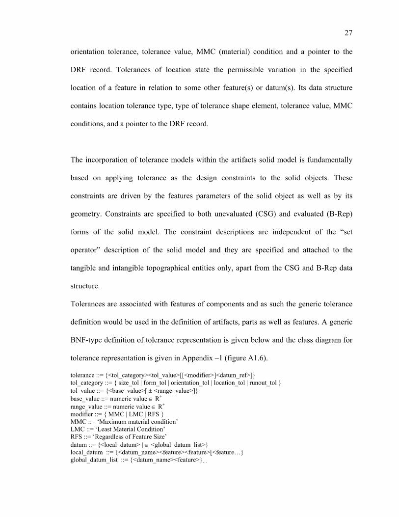
Tolerances are associated with features of components and as such the generic tolerance
definition would be used in the definition of artifacts, parts as well as features. A generic
BNF-type definition of tolerance representation is given below and the class diagram for
tolerance representation is given in Appendix –1 (figure A1.6).
tolerance ::= {<tol_category><tol_value>[[<modifier>]<datum_ref>]} tol_category ::= { size_tol | form_tol | orientation_tol | location_tol | runout_tol } tol_value ::= {<base_value>[ ± <range_value>]} base_value ::= numeric value ∈ R+ range_value ::= numeric value ∈ R+
modifier ::= { MMC | LMC | RFS } MMC ::= ‘Maximum material condition’ LMC ::= ‘Least Material Condition’ RFS ::= ‘Regardless of Feature Size’ datum ::= {<local_datum> | ∈ <global_datum_list>} local_datum ::= {<datum_name><feature><feature>[<feature…} global_datum_list ::= {<datum_name><feature>}…

28
feature ::= <feature_id><feature_type> feature_id ::= a literal name of the feature like F1, F2, etc. feature_type ::={planar | cylindrical | median plane | spherical | conical | others}
The class structures described in this chapter form the basis for the design and tolerance
synthesis schemes discussed in the subsequent chapters.

29
I never saw an ugly thing in my life: for let the form of an object be what it may, - light, shade, and perspective will always make it beautiful.
--John Constable
Chapter 4
Design Synthesis: Function-to-Form Mapping
The design of an artifact to satisfy the product specification (PS) is a complicated
process. The design process is considered evolutionary in nature because we start with
incomplete knowledge about the final product and continue to evolve from a conceptual
design stage to a concrete form/shape. As more knowledge about the product and its
functional requirements are made available, the set of specifications/requirements change
to take into account this new knowledge. In the present approach, suitable functional
entities are searched in the corresponding artifact library to arrive at a starting point for
the conceptual design. At this stage, some of the attributes specified in PS could have
been found and some of the functional requirements may have been satisfied. In order to
proceed further, more knowledge is required to be injected into the system and the set of
specifications need to be transformed for subsequent enhancement of the initial solution.
The design of an artifact is represented as D ::= {<PS><Art_Tree>} where <PS> is
Product Specification and <Art_Tree> is the artifact tree1 (also called assembly graph
and can be treated as a linked list of artifacts).
1 The term ‘artifact tree’ is used here in a somewhat relaxed sense, as the artifact is not a tree in strict graph theoretical definition because there could be loops in the assembly graph - more appropriate term would be artifact graph.

30
The artifact tree is empty at the beginning. Subsequently, as suitable artifacts are mapped
to perform a desired functionality, these artifacts are added to the artifact tree. As the
artifacts in the artifact library (ARTL) has been considered as input-output systems,
outputs from an artifact that are not in the PS become inputs to the next artifacts that may
be added to the artifact during next stage of design evolution. Outputs that could be
mapped in the PS are terminals. Also, the designer may designate an output as terminal
so that further mapping of this output, as input to a new artifact, is not required. This
approach for design synthesis generates stages of (sequence of) partial solutions as shown
below.
D0 = {<PS0><Art_Tree0>} D1 = {<PS1><Art_Tree1>} D2 = {<PS2><Art_Tree2>} … Dn = {<PSn><Art_Treen>}
where <Art_Tree0> is NULL (at the beginning)
At each stages of evolution, the partial solutions are checked for convergence to the
desired output specified in the PS. This checking is performed using two basic criteria: a
constrained norm minimization process involving the relational constraints associated
with the product specification and the individual artifacts. The norm (defined later in this
section) is the ‘distance’ of the partial solution from the desired output. After the
minimization, spatial constraints are checked. Based on the above two process, the set of
candidate artifacts that have been identified, are graded from ‘best’ to ‘worst’ at that
particular stage. A design alternatives control parameter, Nalt as the number of artifacts
(that are most desirable in the graded list) to be considered for the next stage is used to
reduce the search space. This implies that, for example, if in a stage 10 artifacts are

31
mapped and Nalt has been set by the designer as 3, only the ‘best’ three of these 10 will be
used as possible candidates in this stage and searching would continue from those 3 only
for the next stage. It may be noted here that as Nalt increases, possibilities of more diverse
solutions increase. This is a desirable feature because more alternative design solutions
can be explored. However, there is a cost associated with the increase in Nalt in terms of
computation time and storage requirements. In the proposed system, this design control
parameter Nalt has been kept as a designer-selectable value so that the designer can
experiment with different values for Nalt to decide suitable values for specific design
domains.
The design synthesis process at some intermediate stage will have at most Nalt branches
from each of the artifacts in that particular stage. The process of expanding a particular
branch will terminate when one of the following conditions has been reached.
i) A feasible solution satisfying the output specification, relational constraints as
well as spatial constraints have been satisfied. This means that the minimization
process discussed earlier has resulted in an acceptable distance between the
desired output in PS and the partial solution. We designate this acceptable
distance as a convergence criterion, ∈0. Thus d ≤ ∈0 is the termination criteria.
ii) The search for a suitable artifact from the artifact library failed to map at least one
artifact and hence the design synthesis process cannot proceed further.
There are some basic considerations in the design evolution process depicted above that
need further investigations. These are: transformation of PSn to PSn+1, including attribute
transformation, constraint transformations, and variation of internal parameters of each
32
artifact for searching a solution as a minimization process. These have been discussed in
the following sections, before the design synthesis procedure is presented.
4.1 Transformations of Product Specification (PS)
The design evolution process depends on transformation of the Product Specification as
the design progress from one stage to another stage of the design synthesis process. The
PS transformations consist of Attribute Transformation, Constraint Transformation and
the Variation of Internal Parameters as detailed in the following sections
4.2 Attribute Transformation
The product specification PS0 contains the initial specification with PS0.Inp and PS0.Out
as sets of input and output specifications, respectively. Assuming that at stage j, a sub-set
of these sets of requirements have been satisfied, PSj is transformed into PSj+1 as
described below.
Let us assume that an artifact, Artjk has been found in the design stage j with some
elements of Artjk.Inp are in PSj.Inp and some elements of Artjk.Out are in PSj. Out.
We can present this as a union of two mutually exclusive sets
Artjk.Inp = Artjk.Inp1 ∪ Artjk.Inp2 where Artjk.Inp1 ⊆ PSj.Inp and Artjk.Inp2 ⊄ PSj.Inp Artjk.Out = Artjk.Out1 ∪ Artjk.Out2 where Artjk.Out1 ⊆ PSj.Out and Artjk.Out2 ⊄ PSj.Out
If Artjk.Inp2 is NULL then all input requirements of the artifact Artjk are in the product
specification PSj.Inp and this artifact needs no further artifacts whose output should be

33
mapped to inputs. Otherwise, we transform the inputs to a new set of outputs for some
artifact to be searched with:
PSj+1.Out = PSj.Inp ∪ Artjk.Inp2
If Artjk.Out2 is NULL then all outputs of the artifact Artjk are in the product
specification PSj.Out and the outputs of this artifact need not be mapped as input to some
other artifact. Otherwise, we transform these outputs to a new set of inputs for some
artifacts. Here, the designer can accept some of these outputs as by-products to the
environment and treat them as already satisfied. The remaining outputs are then
transformed into a set of new input specification as:
PSj+1.Inp = PSj. Out ∪ Artjk.Out2
4.3 Constraint Transformation
Constraints play a major role in any design by restricting the design search space from an
open-ended search to a more restrictive (and hopefully, of polynomial time) search. In
other words, constraints could be thought of as a guiding mechanism for evolving a
design along some restricted path.
In the present case, constraints have been categorized into three separate categories for
ease of treatment/management. These are: relational, causal and spatial.
Relational constraints are functions relating attributes (or parameters of attributes)
according to some physical law or some other restrictions.
<relational> ::= f(<attribute_name>[,<attribute_name>]…) EQ <value_range>
The function f could be of three types: explicit, implicit or parametric.
<explicit | implicit> ::= f(X) ∈ R, X ∈ Rn

34
<parametric> ::= f(X(t)) ∈ R, t ∈ Rn : tj ∈ (0,1) & Xj = Xj0 + tj* (Xj1 - Xj0)
If f is a vector valued function, it could be treated as a set (f1,f2,…fn) of n scalar functions
such that fj ∈ R , j∈(1,n).
For example, in a rotary motion transformation, a global constraint requiring a speed ratio
(assuming ωI as input and ωO as output rotary speed) could be:
PS.ωI.value/PS.ωO.value EQ (5,6) ; a reduction of 5 to 6 is desired
It has been mentioned earlier, during discussion on artifact representation, that range
(interval) will be accepted as possible values for any parameter. Since relational
constraints are functions involving such parameters, standard interval arithmetic [Moore
(1966)] has been used to treat these types of values. The interval arithmetic that would be
required to deal with ranges of values for attributes for this work has been given in
Appendix –4.
Transformation rule for four basic types of constraints:
Additive: ADD(x,y,z) ::= x + y = z
If x and y then z = x+y If x and z then y=z-x If y and z then x=z-y
Multiplicative: MULT(x,y,z) ::= x * y = z
If x and y then z=x*y If z and x and x !=0 then y=z/x If z and y and y !=0 then x=z/y
Subtractive: MINUS(x,y,z) ::= x - y = z If x and y then z = x-y If y and z then x=y+z If x amd z then y=x-z Functional: FUNC(x,y) ::= y = f(x) , f ∈ M+
35
We will also need another constraint DERIV(x,y) for studying the behavior of artifacts,
derivative: DERIV(x, y) ::= y = dx/dt , f ∈ M+
A constraint defined by f(y1,y2, y3, …yn) = 0 is converted to a set of n equations, by
solving for each yj in terms of the others.
y1 = f1(y2, y3, y4 …) y2 = f2(y1, y3, y4 …) y3 = f3(y1, y2, y4 …) ….
If such an explicit representation is not possible, the constraint may have to be
represented in a different way, either by linearizing about some operating point, or by
approximating into simpler forms.
If an attribute of an artifact is linked/related to another attribute in a linked artifact, two
possible cases occur: an output attribute goes as an input to the next artifact or an input
attribute comes out as an output. In either case, the corresponding component of the
constraint is used and it is solved for the new range for the parameter. This new range
accompanies the attribute as a constraint to the next artifact. In the next artifact, there
may be a priori knowledge about the range of an attribute within which that artifact
operates. In order that the incoming attribute value range is acceptable, intersection of the
two intervals are performed as: Pin ∩ Pallowable. If the intersection is NULL, there is a
contradiction and the constraints associated with the incoming attribute P makes the new
artifact unsuitable for a possible element of the artifact tree.
4.4 Variation of Internal Parameters of Artifacts
As it has been pointed out in earlier in this chapter, artifacts are searched from the artifact
library by matching input parameter types for possible candidates in the solution.

36
However, a suitable measuring and optimizing criteria would be required for guiding the
design solution. In other words, some criteria for selecting the ‘best’ possible candidate at
each stage from a possible set of artifacts have to be formulated.
A ‘distance’ type norm is defined for measuring the proximity between the desired output
(as specified in PS) and the partial solution reached at some stage j, as:
d(a,b) = ( (alow-blow)2 + (ahigh-bhigh)2 ) 1/2
where a and b are two variables representing closed intervals
a = [alow, ahigh] and b = [blow, bhigh]
Above definition satisfies properties of a norm:
d(a,b)=0 iff alow = blow and ahigh = bhigh d(a,b)>0 for a != b d(a,b) = d(b,a)
We would, sometimes, use a parametric form to represent intervals a and b.
As for example, a = alow+(ahigh-alow)*θ : θ ∈ [0,1]
While the range of feasible variations of the input will be used to check for suitability of
accepting an artifact, the variations allowed in the internal parameters of the artifact
would be used to minimize the ‘distance’ between the desired output as specified in PS
and the output (partial solution) at the present stage. The minimization scheme is
formulated as below:
Minimize: d(Oj, O0)
where, O0 is the output specified in the PS and Oj is the output from the artifact j in an
intermediate stage of the design.

37
The partial solution Oj is given by: Oj = fj (Ij, βj), which is derived from the main
constraint C0 (relationship between the input and the output of the artifact j, vide section
3.2.3), by solving for Oj from Cj0 (Ij, Oj , βj) = 0.
The parameter β (where βj = (βj1, βj2,… βjn) ) is the internal parameter of artifact j (vide
section 3.2.3). The parameter β is expressed in parametric form as: βjk = βjk_Low
+(βjk_High - βjk_Low)* θjk : θjk ∈ (0,1), k ∈ (0, n). The subscripts Low and High indicate
the lower and upper bounds of the interval for βjk.
It is also possible that apart from the Co constraint, an artifact may have additional
relational constraints associated with it. These relational constraints are expressed as:
Ck(I, O, β) <rel_opr> <value> , where k>0 and <rel_opr> is the relational operator (one
of {LT LE EQ GE GT NE}), and <val> is a numeric value. For the optimization
scheme, these relationships are converted to the standard equality form Ck(I, O, β) = 0, by
introducing additional variables for the cases where the <rel_opr> is not “EQ”).
The input to the artifact j, Ij is equal to the output from the previous artifact j-1 and so on.
These give rise to the chain of linked equations and the optimization scheme becomes:
Minimize: d(Oj, O0) subject to: ; constraints associated with artifact j Cj0 (Ij, Oj , βj) = 0 Cj,1 (Ij, Oj, βj) = 0 … Cj,c(j) (Ij, Oj, βj) = 0 Ij = Oj-1 ; constraints associated with artifact j-1 Cj-1,0 (Ij-1, O j-1, βj-1) = 0 Cj-1,1 (I j-1, O j-1, β j-1) = 0 … Cj-1,c(j-1) (Ij-1, Oj-1, βj-1) = 0 Ij-1 = Oj-2

38
; constraints associated with artifact j-2 Cj-2,0 (Ij-2, ,Oj-2 , βj-1) = 0 Cj-2,1 (Ij-2, Oj-2, βj-2) = 0 … Cj-2,c(j-2) (Ij-2, Oj-2, βj-2) = 0 … I2 = O1 ; constraints associated with artifact 1 C1,0 (I1, O1, β1) = 0 C1,1 (I1, O1, βj) = 0 … C1, c(1) (I1, O1, β1) = 0
Above minimization scheme could be solved using Lagrange multiplier scheme by
including the constraints into the main optimization function as:
dj = d(Oj , O0) + Σn∈ (1, j) Σk∈ (1, c(n)) (µn,k* Cn,k(In , On , βn)) + Σp∈ (1, j-1) (λp * (Ip+1 – Op))
where c(n) is the number of constraints associated with artifact n, and µ’s and λ‘s are
Lagrange multipliers.
The minimization of dj produces a set of parameters (β*n), for each artifact n ( n ∈ (1 , j)),
which makes the present solution closest to the desired solution. We denote by dj* and
Oj* the corresponding optimal distance and output. If the value of dj*(Oj*, O0) is within a
specified value ∈0 (convergence criterion), we can accept the current design solution
given by Dj = {<PSj><Art_Treej>} as a feasible solution. However, if the distance dj* is
not within acceptable limit, the solution at this stage represents a partial (an incomplete)
solution i.e. the desired output value has not yet been achieved yet.
The above minimization process deals with the relational constraints only. After the
minimization has been performed, (irrespective of the solution whether an acceptable
feasible solution or a partial solution), the spatial constraints are then checked. There can
arise four situations after the spatial constraints are applied.
39
i) A feasible solution has been achieved and the spatial constraints are all satisfied.
ii) A feasible solution has been achieved and all the spatial constraints are not
satisfied.
iii) An incomplete solution has been achieved and the spatial constraints are all
satisfied.
iv) An incomplete solution has been achieved and all the spatial constraints are not
satisfied.
The case i) represents a complete solution and the corresponding branch of the tree can
be terminated without further growth. The rest three cases are incomplete and the
branching / growth of the solution tree continues to the next stage.
4.5 Design Synthesis Process
Before the functional requirements could be transformed into suitable artifacts that could
perform the desired input output transformation, the product specification is searched to
produce a linked list of functional elements that could perform the desired functional
requirements. This process can be represented in a pseudo-code as shown below:
for each functional attribute attrj ∈ Prod_Spec do: { if type(attrj) is input then search function library to locate function fun k , ∃n, ∃k :
funk .type(attrn ) == input AND funk .Category(attrn ) == Prod_Spec.Category(attrj);
else if type(attrj) is output then search function library to locate function fun m , ∃p, ∃m :
funm .type(attrp ) == output AND funm .Category(attrp ) == Prod_Spec.Category(attrj);
endif }
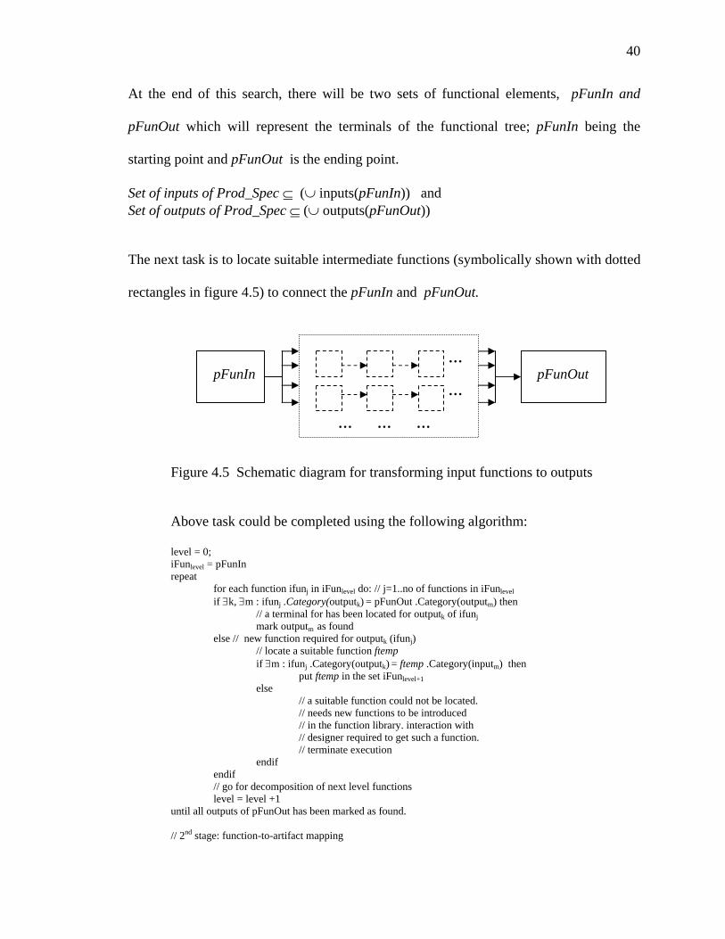
40
At the end of this search, there will be two sets of functional elements, pFunIn and
pFunOut which will represent the terminals of the functional tree; pFunIn being the
starting point and pFunOut is the ending point.
Set of inputs of Prod_Spec ⊆ (∪ inputs(pFunIn)) and Set of outputs of Prod_Spec ⊆ (∪ outputs(pFunOut)) The next task is to locate suitable intermediate functions (symbolically shown with dotted
rectangles in figure 4.5) to connect the pFunIn and pFunOut.
…
pFunIn pFunOut … … … … Figure 4.5 Schematic diagram for transforming input functions to outputs
Above task could be completed using the following algorithm: level = 0; iFunlevel = pFunIn repeat
for each function ifunj in iFunlevel do: // j=1..no of functions in iFunlevel if ∃k, ∃m : ifunj .Category(outputk) = pFunOut .Category(outputm) then
// a terminal for has been located for outputk of ifunj mark outputm as found
else // new function required for outputk (ifunj) // locate a suitable function ftemp
if ∃m : ifunj .Category(outputk) = ftemp .Category(inputm) then put ftemp in the set iFunlevel+1
else // a suitable function could not be located. // needs new functions to be introduced // in the function library. interaction with // designer required to get such a function. // terminate execution endif
endif // go for decomposition of next level functions level = level +1
until all outputs of pFunOut has been marked as found. // 2nd stage: function-to-artifact mapping

41
// In this stage, each of these functional elements would be mapped with a // suitable artifact from the artifact library to achieve the desired functionality. // The steps for the artifact library search is described in the design synthesis steps // below
The steps in the design synthesis process could be represented as below: 1. Start with a product specification (PS) and a null design object D. 2. Take an attribute from the PS (PS.Attrj) and locate a set of artifacts from the artifact library(ARTL) each having
the same category of attribute as in DP.Attrj.
For all artifacts in ARTL Do: If PS.Attrj.type = ARTL.artk.attrm.type AND PS.Attrj.category = ARTL.artk.attrm.category then // an artifact is found, save the pointer in DTemp endif
End Do
If Dtemp is NULL then no artifact could be found If all attributes are checked then Exit loop 2 else Check with the next attribute PS.Attrj+1 endif Else
Exit loop 2 // at least one artifact has been found! Endif
3. If Dtemp is NULL then
// consult a functional equivalence (FE) class library (which is defined based on the design domain- specific knowledge) to try to replace a functional requirement with a set of functions that can collectively perform the desired functionality. Modify the PS accordingly and continue with loop 1. // if all such functional equivalences have been exhausted and even then none of the attributes in PS could map a suitable artifact from the ARTL. The PS needs futher refinement, addition of new attributes and / or addition of new artifacts in the ARTL.
Terminate.
Endif
Apply the constraints associated with PS.Attrj to all the artifacts in Dtemp. If Dtemp contains more than one artifact then
Apply heuristics to select the ‘best’ N artifacts (N>=1, specified) // note N>1 means we continue with more than one artifact that has been found.
/* This would be a desirable feature from ‘getting variety of alternative designs’ point of view. Also, though the constraints for the attribute may be ‘best’ satisfied for one artifact, other artifacts with partially satisfied constraints may lead to better alternative designs. This is due to the fact that some global constrains and goals which could not be checked / applied at this stage, may be better satisfied after all the functional requirements have been found. However, as N increases, the solution space expands rapidly, and may be restrictive from computational point of view. This aspect has to be studied further to decide reasonably good upper bound on N.
*/ Endif

42
4. Althouh N could be more than 1, henceforth we proceed with one alternative from the Dtemp. Identical procedure will be applicable for all the alternatives. Let D1 = Dtemp.Art1 Modify the attribute values with those in PS and percolate the constraints. The design space D now contains one artifact. In general, this artifact will have other attributes and constraints associated with it. Now, in order to consider this artifact as an element of the solution D, these are also to be considered as part of the design specification. Thus we will now augment the design spec PS with the unsatisfied attributes of this artifact. Let DI = set of input parameters of D1.Atr1 DO= set of output parameters of D1.Atr1 If some of the elements of DI and DO are already in PS, we mark them as found otherwise, and remove them from DI & DO. The remaining attributes need to be satisfied. Since both the above two sets were not a desired requirement, we would put a negative weight to these attributes (undesirable?) and augment the PS with these new sets of attributes along with associated constraints. We will now search for artifacts from the ARTL by transforming the DI and DO as: Generate a temporary sub-design spec with input attributes = DO and output attributes = DI // input DI to D1.art1 must come as output of some other artifact or from a terminal which we also consider as artifact with no input and one output (like an electricity supply point as a terminal that supplies electric energy and need no further input) // output DO from D1.art1 must either be accepted as an undesireble by-product to the neighborhood and no further exploration would be required or the output must be mapped as in input to some other artifact. The solution D1 is now copied as D2 and next search proceeds. This search would be identical to the one carried out in section 2 above. Thus at each stage of evolution of design solution, further artifacts would come in the D’s and the solution will grow in many directions. We will keep track of each stage of solution along with corresponding product spec in a stack as:
{<D0,PS0>,<D1,PS1>,<D2,PS2>,…,<Dn,PSn>} The process will terminate when one of the following is satisfied. 1. All the attributes in the PS has been found: In this case, a feasible solution has been found. Now, the solution
Dn the global constraints and goals could be evaluated. 2. Some of the attributes are yet to be found and no further artifact could be located in ARTL. In this case,
either the designer will provide some more domain specific knowledge in the PSn or some new artifacts would be added to proceed further. However, in order to explore other possible solutions, we may backtrack one step to <Dn-1, PSn-1> and consider other less favorable possibilities.
Above procedure is described in the following steps:
0. Develop design domain specific artifact library (ARTL), functional equivalence
library (FUNL) and domain-specific knowledge base (DK). For the time being,
we assume that the DK is specified in the form of constraints and relations in the

43
PS itself. However, these could be separated out for treating them in a generic
way.
1. Start with a product specification PS.
2. Locate suitable artifacts from the ARTL mapping the input parameters from the
product specification with those of the artifacts having same input type. If no
artifacts are found, go to step 8.
3. Check whether the type of output from some of these artifacts matches the output
types specified in PS. Divide the artifacts into two sub-groups: one with artifacts
whose output matches the desired output (DM) and other where such a match is
not found (DNM).
4. a) With DM
Generate the distance function between the output and the desired output in PS
and minimize the distance along with the constraints associated with the
attributes.
1. If the distance for some of the artifacts are within a specified acceptable value,
a possible solution has been found.
2. Apply the spatial constraints to these artifacts. If these constraints are
satisfied, go to step 10
3. If the distance is not within the acceptable value, only a partial solution has
been found. Take the top Nalt artifacts nearest to the solution. Go to step 5.
b) With DNM
44
In this case, the minimization criteria cannot be applied yet since the output type
did not match the desired output type in the PS. The minimization scheme can
only be applied when a match for the desired output has been found. Proceed to
step 5.
5. Generate new sets of attributes and transform the constraints to augment the PS so
that additional attributes associated with the selected artifacts could be taken into
account.
6. Repeat steps 2 to 5 with transformation of the product spec PS.
7. Continue untill such time the entire attribute requirements are satisfied or some
attributes could not be mapped.
8. At any stage, if some attributes could not be mapped, there would be three
alternatives: look for a possible functional equivalence class and modify the PS
accordingly and continue search. If such a functional equivalence class is not
found, consult with the designer to acquire new attributes, knowledge, constraints
and/or modify existing specification. Repeat steps 2-5 after such modifications. If
above steps still fail to map some attribute requirements, the designer needs to add
new artifacts in ARTL and/or add new functional equivalence classes in Function
Library. After this step, repeat the process again.
9. In case all options have been exhausted at an intermediate stage, and a feasible
solution has not been found, consider the possibility of going back one step
(backtracking) and consider other less favorable paths with artifacts with lesser
matches.

45
10. After a feasible solution has been found, a tentative sizing of the components of
the artifacts is carried out by using the attribute values specified and by applying
the physical laws governing the behavior of the artifact. If during this process,
some parts could not be sized within acceptable range of values, consider possible
change of the PS and go to step 7.
11. Introduce tolerance models associated with each artifact in the artifact tree and
carry out tolerance analysis. If during this process, tolerance requirements for
some parts are not feasible, consider changing PS and go to step 7.
12. Consider manufacturability of the artifacts in the design solution. Apply criteria
for manufacturability. If during this process, some manufacturing requirements
for some parts are not feasible, consider changing PS and go to step 7.
13. Consider global goals and constraints associated with the product specification. If
the global constraints are satisfied, initiate global optimization processes and
consider changing the PS again to achieve some global goals and go to step 7.
14. A feasible design has been found.
The iterative design synthesis process will terminate when one of the followings is
satisfied.
1. All the attributes in the PS have been found and the desired output value level has
been achieved. In this case, a feasible solution has been found. Now, the global
constraints and goals could be evaluated.

46
2. Some of the attributes are yet to be found and no further artifact could be located
in ARTL. In this case, either the designer will provide some more domain
specific knowledge in the PSn or some new artifacts would be added to proceed
further. However, in order to explore other possible solutions, we may backtrack
one step to Dn-1 and consider other less favorable possibilities.
4.6 Observations on the Design Synthesis Process
In general, an artifact may have more than one input and output attribute and constraints
associated with them. In order to consider the artifact as an element of the solution, these
attributes are also to be considered as part of the design specification. Thus, we need to
augment the design specification with the unsatisfied attributes of this artifact.
If some of the input and output attributes are already in PS, we mark them as found the
remaining attributes need to be satisfied. Since these inputs and outputs were not in the
original product specification, they are not desirable from the product specification
requirement. However, these must be mapped to other artifacts. We would put a negative
weight to these attributes (undesirable?) and augment the PS with these new sets of
attributes along with associated constraints.
With this augmented PS, we will now search for artifacts from the ARTL. The input
attributes must come as output from some other artifact or from a terminal that we also
consider as artifact with no input and one output (like an electricity supply point as a
terminal that supplies electric energy and need no further input)

47
The output attributes must either be accepted as an undesirable byproduct to the
environment and no further exploration would be required or the output must be mapped
as in input to some other artifact.
As an example, the above proposed design procedure has been applied to a simple design
problem and the steps have been elaborated in the next section.
4.7 An Example of Design Synthesis
Design problem statement: Design “a device to increase the rotational speed by a factor
of 10”. The product specification is as below:
PS = ( (function rotation to rotation) (input wI rotary_motion rad/sec 0 wi0) (output wo rotary_motion rad/sec 0 wo0) (constraint relational wo = wi / 10) (constraint spatial (axis(wI) parallel_to axis(wo)) // some other attributes, not essential for the example have been left out.
)
Let PS0 = PS. The design is started with PS defined above and solution
D0 = ({PS0}, {null})
To make the example easier to follow, we will use Ai,j to indicate artifact Ai as used in
stage j
The attribute PS0.wI is an ‘input’ and the type of the ‘input’ is ‘rotary_motion’. Searching
the artifact library ARTL, we find artifacts {A1, A2, A3, A4, A5, A6, A7, A8} all having
the same ‘input’ category with ‘rotary_motion’ as type. Hence D0 = ({PS0}, {A1, A2, A3,
A4, A5, A6, A7, A8}). The set of artifacts {A1, A2, A3, A4, A5, A6, A7, A8} can satisfy the
‘input’ requirement. Thus we set,
D0=({PS0}, {A1,0, A2,0, A3,0, A4,0, A5,0, A6,0, A7,0, A8,0})

48
There are no more ‘input’ category attributes. We now check whether the outputs of these
artifacts match the output specified in the PS. We find that artifacts {A4,0, A6,0, A7,0}
meets this requirement. Thus, at this stage, we have two distinct subsets of D0 , D01=
({DP0}, {A4,1, A6,1, A7,1}) and D02 = ({DP0} {A1,1, A2,1, A3,1, A5,1, A8,1}). While each
artifact in D01 can meet both input and output requirements of PS, those in D02 only meet
the input requirement.
The two sets D01 and D02 require different treatments and we split the design synthesis
into two segments.
Segment #1: With D01
Since both input and output requirements have been found, we apply the
constraints and see how far the constraints are satisfied:
For artifact A4,1:
Its internal relationship is: wO = wI * R, where R=[0.25,4.0]
In parametric form, it becomes R = 0.25+3.75*θ, where θ ∈ (0,1).
Minimization scheme: minimize d(PS0.wo, D1.A4.wo)
d = d(10*wI, (0.25+3.75*θ)*wI)= wI*(9.25-3.75*θ)
θ* = 1.0 for minimum d = 4*wI.
With this θ*, d is not yet zero, so the artifact A41 can only meet the output
requirement partially. We need to add some other artifacts to the artifact 4 to
reach the desired output. In this stage, with (θ*, wo*) = (1, 4.0 * wi )
Similar computations with artifact A6,1 and A7,1 also leads to incomplete
fulfillment of the desired output level, which are (θ*, wo*) = (1, 3.0 * wi ), (θ*, wo
*)
= (1, 4*wI) respectively.

49
Now, applying the spatial constraints, we see that:
Art A4,1: axis(w1) parallel_to axis(w2) IS TRUE Art A6,1: axis(w1) parallel_to axis(w2) IS TRUE
Art A7,1: axis(w1) parallel_to axis(w2) IS FALSE
Thus, at this stage, by considering above two constraints (both relational and
spatial) satisfaction criteria, we grade artifact A4,1 as the most appropriate artifact,
followed by artifact A6,1 and artifact A7,1.
For the next stage, in order to search for new artifacts that can take outputs from
the above 3 artifacts (artifacts {A4,1, A6,1, A7,1}), we transform their corresponding
outputs to the desired inputs for the new artifacts.
The spatial constraint has been satisfied for artifacts A4,1 and A6,1 and would need
no further transformation; however, the spatial constraints for artifact A7,1 has not
been satisfied and needs to be transformed as: axis(w1) perpendicular_to axis(w2).
This is because the current unsatisfied constraint axis(w1) parallel_to axis(w2) (an
angle of zero) could not be met. The constraint axis(w1) perpendicular_to axis(w2)
(an angle of 900 ) is converted to axis(w1) perpendicular_to axis(w2) (an angle of
900 ), so that the combined effect of another artifact which meets this requirement
would produce 0 or 180 as parallel, the final requirements.
With these modified specifications, we carry out the search again.
First we take the case of artifact A4,1 and find that all the artifacts A1 - A8 can
take the corresponding output as input.

50
Applying the same procedure as it was followed in the previous stage, we come
across artifacts D2= {A4,2, A6,2, A7,2} as possible candidates. Applying the norm
minimization criteria:
For Artifact A4,2:
Its internal relationship is: wO = wI * R, where R=[0.25,4.0]
In parametric form, this becomes R = 0.25+3.75*θ, where θ ∈ (0,1).
Minimization scheme: minimize d(PS0.wo, D2.A4.wo)
d = d(10*wI, (0.25+3.75*θ)*4*wI)= wI*(10-1-3.75*4*θ)
(θ*, wo*) = (0.6, 2.5 * wI) for minimum d=0.
Thus, D2 = ({{PS1}, {A4,1}}, {{PS2}, {A4,2}}) is a solution that meets the output
requirements.
Applying similar optimization criteria to the other two artifacts A6,1 & A7,1, we get
optimal solutions as: (θ*, wo*) = (1.0, 2.0 * wI) and (0.6, 2.5 * wI) respectively.
The corresponding distances are 2*wI and 0 respectively. Now applying the
spatial constraints,
Art A4,2: axis(w1) parallel_to axis(w2) IS TRUE Art A6,2: axis(w1) parallel_to axis(w2) IS TRUE
Art A7,2: axis(w1) parallel_to axis(w2) IS FALSE
Thus after this stage, one feasible solutions (A4,1 A4,2) and a partial solution
(A4,1 A6,2) have been found. For the third combination (A4,1 A7,2), though the
distance is zero, the spatial constraints are not satisfied.
Same procedure with artifacts A6,1 and A7,1 from stage 1 leads to the following
situations: (A6,1 A4,2), (A6,1 A6,2), (A6,1 A7,2) as partial solutions and

51
(A7,1 A7,2) as a feasible solution. The process could be continued till the desired
output criteria are met.
A part of the design process is shown in figure 4.7-1 where Anj indicates the
artifact number n in the ARTL as used in design stage j. Some of the solutions
found have been shown in figure 4.7-2

52
A1,1 A1,2 A2,1 A2,2 A3,1 A3,2 A4,2 A solution (A41 A42) <PS0, D0> A4,1 A5,2 A5,1 A6,2 A7,2 A6,1 A7,1 <PS1, D1> <PS3,D3> <PS2, D2>
Figure 4.7-1 Design Synthesis Process- some intermediate stages from the example
A1,3
A2,3
A3,3
A4,3
A5,3
A6,3
A7,3
A1,4
A2,4
A3,4
A5,4
A7,4
A solution (A6,1 A4,2 A4,3 A4,4) A4 4
A solution (A6,1 A4,2 A6,3)A6 4
A1,2
A2,2
A3,2
A5,2
A7 2
A4,2
A6,2
A solution(A7,1 A7,2)

53
Input Output
Solution A4,1 A4,2 Input Output
Solution A4,1 A6,2 A4,3 Input Output
Solution A7,1 A7,2
Figure 4.7-2. Typical Solutions from the Design Example

54
Segment #2: With D02
The next process is applied to D02, where the output is not the desired output specified in
PS. In our example, we have the set D02 = ({DP0} {A1,1, A2,1, A3,1, A5,1, A8,1}).
Since these artifacts do not produce the desired output type (i.e. rotary_motion) as
specified in PS, we cannot apply the relational constraints specified in the PS. However,
we can apply the spatial constraints as well as any local constraint associated with the
artifacts, to eliminate some of the artifacts or to assign lesser importance to the artifacts
of the set D02. After the constraints have been checked, we transform the outputs and the
spatial constraints to search for artifacts, which can take these outputs as input attributes.
If some artifacts could be found, we proceed as it has been stated in Segment #1.
However, if nothing could be found, we consult the functional equivalence knowledge
base library to check if suitable functional equivalence could be identified that can
decompose this output into a collective group of functions. If such functions are found,
we continue the search with the new set of inputs to locate some artifacts. If some
artifacts are found, we proceed as before. If no such function is found, the design process
stops at this stage and further input is required from the designer. There are three
possibilities: inject some more design specific domain knowledge either in the PS or in
the functional equivalence class library, or add new artifacts.
It may be noted here that the sample artifact library and the functional equivalence class
library developed for this design example have no such artifacts. And the design process
in this Segment ended here without any feasible solutions with D02.

55
It is postulated that after a finite number of steps, a set of artifact chains will be found, the
final element of which has the desired output type. Now, the relational constraints could
be applied and the internal parameters of the artifacts could be optimized to see if the
desired level of output has been reached. This problem then becomes a multivariate
minimization with constraints.
The minimization process assigns optimum values for the internal parameters of each
artifact. After the minimization, if the distance d is within a specified value of ∈0, the
solution has converged to a feasible solution. However, if d is still not within the range,
we continue to add another possible chain of artifacts, and optimize. The process is
repeated until the desired level has been reached.

56
He who wonders discovers that this in itself is wonderful. -- M. C. Escher
Chapter 5
Tolerance Synthesis Scheme
Tolerance synthesis is the process of allocating tolerances among the geometric
parameters (dimensions) of the parts/components such that some costs associated with
the artifact is minimized and at the same time the functional, manufacturing, and
assembly requirements are satisfied. The generic tolerance model that has been defined in
chapter three is used in this chapter to represent tolerances associated with features of
parts of an artifact. However, as has been mentioned in chapter one, traditional tolerance
representation (per ASME Y14.5M,1994) schemes are not directly used in the tolerance
synthesis (TS) scheme as such representations are not suitable for uniform treatment in a
generic manner. For the TS scheme a detailed description of the “kinematic functions” of
the product assembly are required. These essentially mean functions defined by the
location, size and shape (form) of associated mating parts/features of the artifact. These
functional specifications are not directly provided by the customer or by the designer at
an early stage of design. They are slowly evolved with the assembly as the design takes
concrete shape and size in the later phases of the conceptual design. Tolerance synthesis
and analysis need an exhaustive functional analysis mechanism to make sure that the
identified functional requirements between the mating components of the assembly are
met and are suitably described in the form of critical toleranced dimensions / size / sizes /
forms. In this tolerance representation scheme the small deviation torsor (SDT) scheme

57
[Ballot (1998)] has been used to represent the variations associated with each feature of a
part in the assembly. In subsequent sections details of steps involved in the TS has been
elaborated.
5.1 Representation of Deviations of Features of a Part
The geometric variations of a feature are defined in terms of deviations of the
independent degrees of freedom of the feature. In this approach, at the most six
independent parameters are required to represent a six-component vector corresponding
to the possible six degrees of freedom. In actual case, depending on the type of surface
(planar, cylindrical, etc) some of the degrees of freedom are ‘free’ (variations along
which keeps the surface invariant) and thus, in general, less than six deviation parameters
are required to represent the behavior of a feature. For example, for a planar surface,
rotation along the outward normal to the surface and movements along the two axes on
the surface keeps the feature invariant and hence a planar surface requires only three
deviation parameters (axial movement, two rotations along the two transverse axes).
In order to make the process of converting the functional requirements as well as
kinematic requirements into a set of constraints in a generic manner, a procedure is
needed to represent the variations associated with each part in terms of a set of
parameters of the mating features/surfaces. Assuming small displacements (deviations) of
these features due to manufacturing inaccuracies and/or other defects, the actual surface
of a feature deviates from the theoretical (nominal) surface slightly. Such variations could
be systematically treated by considering variation of six small parameters defined at a
58
point on the surface. The six parameters are: three linear translations and three rotations
along the three axes of a local orthogonal coordinate system corresponding to the six
degrees of freedom. These six small displacement parameters are called screw
parameters or torsors.
In general a feature of a part embedded in 3-D space would have six degrees of freedom
(DOF): three linear, three rotational. In other words, six parameters could be used to
represent the deviation of a feature from its nominal position. In fact a tolerance specified
for a feature is nothing but some deviation of the nominal feature with reference to a
datum or it could be an intrinsic variation. These deviations are small compared to the
dimensions of the part and these deviations of a feature could be accurately described by
two vectors: a three-component displacement vector and a three-component rotation
vector defined at a convenient point on the feature. Each vector is assumed to have a very
small norm. These two components in a collective form are called a small displacement
torsor (SDT). Assuming the two vectors are represented by: small displacement d = (dx,
dy, dz)T and small rotation θ = (θx, θy, θz)T , the SDT can be written as: T=(θ, d)T = (θx,
θy, θz , dx, dy, dz)T. Although a torsor looks like a six component vector, its transformation
rules (Appendix 5) are different because the two 3-component vectors are not compatible
quantities. One represent linear displacement while the other is a rotation vector.
For representing the deviations of a feature, first a suitable point of interest is chosen on
the feature and the six components of the torsor is defined at that point as quantities in a
local coordinate system. Although there is no preferred point as any point on the feature

59
could serve as a reference point, from practical design point of view, often points are
chosen on specific locations on the feature for ease of coding and interpretation. For
example, a point at the center of a rectangular planar feature could be preferred. Apart
from choosing a point of interest, we also need to define a local coordinate system (LCS)
at that point. The process detailed below could be used to define the LCS.
5.1.1 Local Coordinate System on a Feature For features defined by parametric surfaces of the form f(x) = 0, we assume f to be at
least piece-wise continuous and it’s gradient (∇f) could be computed at a point where we
would like to define the deviation parameters. Since the development of the
assemblability constraints doesn’t depend on the point where we define the deviations
(although the equation changes as the torsor transformations are dependent on the spatial
coordinate of the point), we can choose arbitrary point on the feature surface. However,
often it becomes reasonable to choose points that can be thought of as natural candidates
for ease of interpretation of results as well as manipulation of deviations at these points.
For example, if the feature is symmetric (for example, circular, rectangular, square
features), the geometric center could be taken as the ‘point of interest’. So the selection of
strategic points could be left to the designer/user without affecting the computational
complexity.
After a suitable point ‘P’ has been selected (figure 5.1.1), the LCS is defined as below:
Compute the gradient of the surface at P: ∇f=(∂f/∂x, ∂f/∂y, ∂f/∂z) Normalize ∇f: ∇f=∇f/||∇f=||. Compute the dot product of dX and ∇f: λ= dX.∇f, where dX is a vector from an interior point (material side of the part to which the feature belongs) to the point P. If λ is positive then
∇f is outwards (emanating from the material side, which is what we want) else reverse the sign of ∇f
∇f = -∇f

60
endif Take local-x = ∇f. If the local-x = global-x then
local-y=global-y and local-z = global-z else if local-x=global-y then
local-y=global-z and local-z=global-x else if local x=global-z then
local-y=global-x and local-z=global-y else
Generate local-y by taking a unit vector on a vertical plane containing the local-x and making it perpendicular to local-x.
end if
Generate the local-z as cross product of local-x and local-y.
Figure 5.1.1 Local coordinate system on a feature
Above procedure generates the desired right-handed local coordinate system for defining
the deviation parameters at that point.
5.1.2 Invariants of a Feature and Reduction of DOF
Although we start with six components for each SDT, we can eliminate some of the
components depending upon the type/nature of the feature. This is possible because most
features used in engineering applications are regular. Because of this regularity there
could be some DOF that act as invariants for the feature. For example, for a cylindrical
feature, there are two such invariant parameters: axial rotation and axial movement. Both
of these deviations keep the cylindrical feature invariant. Thus these two parameters
could be eliminated. This leads to a four component deviation for a cylindrical feature
P x
y
z

61
with an axis along the x-axis: ((0, θy, θz), (0, dy, dz))T. Similarly, for a planar feature, with
z-axis along the normal to the plain (the deviation parameters are defined at point P, at
the center of the feature, figure 5.1.2), θz, dx and dy are invariants, which makes it
possible to represent the deviations of a planar feature with three parameters: ((θx, θy, 0),
(0, 0, dz))T.
Figure 5.1.2 Deviation parameters of a circular-planar feature
Apart from the deviation parameters defined at the point of interest, another torsor is
required to represent the possible overall rigid body displacement of the part as a whole.
Thus in general two torsors are needed to completely define the position of a feature. One
for the displacement of the part on which the feature is defined – called displacement
torsor that we conveniently define at the center of a part, and the other to represent the
intrinsic (local) variation of the feature called intrinsic torsor.
5.2 Tolerance Synthesis (TS) Scheme
The TS scheme has been formulated as a constrained non-linear optimization process and
following steps are required to realize the TS scheme:
DP = (θx, θy, θz , dx, dy, dz)T DP = (θx, θy, - , -, -, dz)T
X
Y
Z P
Y
P

62
1. For each component of the artifact, develop the kinematic DOF requirement
between the mating features and decide the intrinsic displacement and deviation
of the feature from the nominal surface as torsor components.
2. For each pair of connected features, establish the gap between the features as a
gap torsor taking into account the indeterminate and/or blocked degrees of
freedoms.
3. Generate assemblability constraints (geometric compatibility) by considering all
chain of connected components as a kinematic link (either closed loop or path
between two datum features) and aggregate the deviations (torsors) along the path
with reference to a global frame of reference. Each loop generates six equations
binding the deviation parameters associated with all the related features. These
sets of constraints would form a deviation hull for the possible geometric
variations of the connected components.
4. Generate constraints for functional requirement based on the specified
functions/objectives to be fulfilled by the artifact. This will restrict the range of
values of the deviations within which a component must remain to fulfill specific
functional requirements.
5. Generate manufacturing / production costs models for each component (based on
suitable knowledge base for manufacturing / production cost) for different
machining operations and formulate a minimization scheme by considering the
sum of costs for machining all the parts as the cost function subject to the
constraints defined in steps 3 & 4 above.

63
6. Use standard mathematical tools to solve the above optimization scheme to find
the deviation parameters for each component.
7. Convert the optimal deviation parameters associated with each feature into
appropriate tolerance zones through deviation-to-tolerance mapping.
Above steps are elaborated in the following section.
5.3 Deviation of Features and Assembly of Mating Parts
The TS process is based on generic deviation parameters that define the deviation of
features in the assembly of pats. The process of allocation/assignment of suitable torsors
for each mating feature is illustrated using an example. The example has been taken from
the design evolution example shown in chapter four where the design evolution process
was illustrated by taking an example of designing a device for transmitting torque with
changing rotational speed. One of the solutions is taken from the above design example
and for the following a tentative sizing of the components as assumed.
The gear-subassembly consists of three parts: a spur gear, a shaft with a keyhole and a
key. The geometric models of these three parts, including their feature-level mating
relationships are shown in figures 5.3-1, 5.3-2 and 5.3-3. The last figure is the assembly
graph of the gear sub-assembly showing logical connections between features. A typical
feature of a part is labeled <PnFn> where P stands for part, F stands for feature and n is
serial number of the part/feature. Thus P3F2 indicates the 2nd feature of part 3.

64
Figure 5.3-1 A spur gear sub-assembly
Figure 5.3-2 Mating details of the gear sub-assembly
Key
Gear
Shaft

65
Figure 5.3-3 Assembly graph of the gear sub-assembly
As it has been detailed earlier in section 5.1.1, a suitable point is chosen on each feature
and deviation torsor components are defined at that point to represent the deviation of the
feature in a local coordinate system defined at that point. Based on the type of feature,
torsor components suitable for that feature are selected for each of the mating features.
After this operation, the assembly graph of the artifact (Figure 5.3-3) is constructed by
connecting features/parts that are in mating. The assembly graph is then traversed to
generate all independent paths between two terminals* and closed loops by an exhaustive
search (details of the search procedure, special techniques to identify inner loops, and
procedure to eliminate duplicate reverse paths have been discussed in the implementation
section of chapter six). Each independent path is then used to generate one set of six
constraints for assemblability (geometric compatibility) by aggregating the torsors along * Terminals are datum features or features of a part with known deviations that could serve as an anchor.
66
the path using the torsor transformation and summation rules. This is similar to traversing
a vector loop. Union of all such constraints represents the configuration hull (various
possible geometric configurations) for the artifact. This procedure has been elaborated
further during development of assemblability constraints in section 5.4.2.
For computations in each loop, the local variations are to be converted to a global
coordinate system by transformation of the corresponding torsors in the local frame.
5.3.1 Gap as a Control Element between Mating Features
While traversing these paths, the gap between the two mating features is used as a control
element that could be effectively used in deciding the type of interface between the two
mating features. The gap between two features is modeled using a gap torsor and the
deviation parameters of the gap is used to generate constraints for the functional
requirements that is local to the two mating features (section 5.4.1).
5.3.2 Shifting the Point of Interest
The deviation parameters for a feature are conveniently defined at a suitable point for
ease of interpretation and understanding. However, there could also arise needs to assess
the possibility of any interference between the mating features at other different points.
This checking is done by transforming the torsor from one point to another by applying
the torsor transformation rules. This would require studying the torsor equations applied
at those strategic points. These points could also be conveniently used for inspection of
the features after manufacturing. The artifact class contains attributes for keeping track of
these points so new points could be added as required for specific surfaces/features. For

67
example, in case of a rectangular feature, four furthest points (corner points) could be
selected as the desired points and for circular features, eight points uniformly distributed
on the circumference could be kept (figure 5.3.2). It may be mentioned that additional
points as desired may be introduced at any stage to improve accuracy; however, the
number of equations & complexity of the problem would increase with each additional
point.
Rectangular: 4 points @ 4 corners Circular: 8 points @ equal intervals
Figure 5.3.2 Points of interest on features.
After all the loops have been considered and corresponding equations have been formed,
we get a system of equations that will define the possible geometric variations of the
artifact configuration. Depending on the type of mating and functional requirements for
each mating pairs of surfaces, these sets of equations may be under or over constrained.
In other words, there may be too few equations connecting too many variables or vice-
versa. These will constitute the constraints of the optimization process for tolerance
synthesis.
5.4 Generation of Constraints
There are two different categories of constraints associated with the tolerance synthesis
process: a) constraints for meeting the functional requirements of the artifact and b)

68
constraints to meet geometric mating compatibility (assemblability). Since both the
constraints play crucial roles in the tolerance synthesis process, each process have been
elaborated separately in the following sub-sections.
5.4.1 Constraints Related to Functional Requirements
Functional requirements are design requirements specified explicitly as well as implicitly
by the user and designer to meet certain desired performance from the artifact. In terms of
tolerance and deviation parameters these functional requirements would translate into
constraint i.e. functions establishing some mathematical relationship between the
parameters.
Functional requirement can be described:
a) Either, as a goal satisfaction to minimize a penalty cost for deviating from the
design specification
In this case a functional requirement defined by some function fj(x) ≤ f0j,
where x is the deviation parameter, could be added to the cost function as a
penalty cost using Lagrange multipliers, for example, λj * abs(fj(x)-f0j)
b) Or, as a set of constraints on the tolerance zone
In this case the functional requirements fj(x) ≤ f0j would be used as non-linear
constraints for the cost optimization.
Since the functional requirements are developed to represent customer’s specification and
designer’s technical requirements, it is desirable to satisfy these constraints as necessary
69
constraints rather than treating them as penalty costs. Thus, the functional requirements
have been treated as constraints (functions of deviation parameters of the mating features
of the components). The functional requirements generally translate into algebraic
inequalities representing constraints of the form: G(x) ≤ 0, x ∈ Rn
As mentioned earlier, functional requirements specified between two mating features
could be conveniently represented by using the deviation parameters of the gap between
the mating features. Although a generic transformation rule couldn’t be found because
these requirements are domain dependent, constraints of the general form as given above
could be treated as functions of the gap parameters only. For example, if a designer
specifies that a minimum gap of 0.0025 must be maintained between a rotating shaft and
the bearing to minimize friction, this requirement could be specified by using a constraint
using the gap element between the two cylindrical features (shaft and hole) as: Gijx ≥
0.0025, where Gijx is the local x-component of displacement (radial component) of the
gap element between the two mating features i and j. More complex requirements could
be represented with appropriate functions.
5.4.2 Constraints Related to Assemblability of Parts
Parts are assembled in an artifact to facilitate transmission of energy / force / motion /
fluent through the mating features. Sometimes parts are used to block some of the above
entities as well. These requirements could be treated as kinematic constraints on the DOF
between the mating features. These constraints represent geometric compatibility
(assemblability) because pair of parts must mate as per specified to serve the desired
function.

70
These assemblability constraints are established by considering sum of torsor components
along each independent paths/loops that exist between datum features. The torsor
summation is carried out using the torsor transformation rules by transferring the effect of
a torsor from a local point to another point on the datum. In the small displacement
assumption, the assemblability constraints become linear and can be put in the compact
form: Kx = b, where K = [kij] is a m x n matrix, kij ∈ R, x ∈ Rn , b ∈ Rm (b is
formed from known deviations of the features), and m is the number of constraints.
In the derivation of the K matrix we assume without any loss of generality and without
any ambiguity that each loop/path in the assembly graph could be enumerated as a linked
list L defined by:
L = {(p, f), g, [(f, p, f), g]…, (f, p)} … (5.4.2-1)
where p denotes part, f denoted feature, g denotes gap between mating features and items
shown within [ ]… could be repeated zero or more times as required to traverse a
loop/path.
(p, f) is the starting point (from_part, from_feature)
(f, p) is the end point (to_feature, to_part)
[(f, p, f), g] are intermediate connections (to_feature, part, from_feature), gap) along the
path to the next part. This is elaborated in figure 5.4.2

71
Figure 5.4.2 Traversing Paths/Loops in an assembly graph.
In case of a closed loop, the last part would be the same as the first part. Both the starting
and the final parts for open loops should be terminals (datum). In case of closed loops,
the summation of the torsors would be null (0), whereas for an open path, the summation
would be equal to a torsor (possibly non-null) that has to be established from known
functional specifications between the two terminal parts. This quantity is designated as b.
T has been used to represent torsor with index p, f, g for parts, features and gaps
respectively. Let
Pj = Part number j, j =1 to n, n = number of parts in the loop
Fk = Feature k of part Pj , k = 1 to m, m = number of features of part Pj
Tp = 6-component displacement torsor of the part P, defined at a suitable point O
inside the part in a local coordinate system. Tf = 6-component deviation torsor of the feature k, defined at a suitable point N on the
feature in a local coordinate system with x-axis along the outward (away from the material) normal and y & z are the other two axes mutually perpendicular to the x-axis.
Tg = 6-component gap torsor defined at a mating between two features of two parts.

72
With the above notation, we can write the desired equations for each loop, with implied
local to global transformations applied to each torsor as viewed from any convenient
point (typically, at the center of the first part where the loop begins), as:
(Tp + Tf ) + Tg [-Tf -Tp + Tf + Tg )]… (- Tf - Tp ) = b … (5.4.2-2)
where the plus (+) sign indicates going out from a feature/part and negative (-) sign
indicates entering a feature/part.
Summing over the entire loop, and using the torsor transformation rules (Appendix 5),
the above equation could be converted to the following form:
∑∈
=×∆+EntireLoopj
jjjj bxK
)(* δθδ … (5.4.2-3)
and
θθ bKEntireLoopj
jj =∑∈
* … (5.4.2-4)
where, Kj is the local to global transformation matrix (Appendix 5, eqn.A5-3) for feature j δj = [δx δy δz]T
j and θ j = [θ z θ y θ z]Tj are the two vectors formed from the linear &
rotational components respectively of the deviation torsor of the feature j. ∆xj =(∆x, ∆y,
∆z)T = (Xj-X0, Yj –Y0, Zj-Z0)T is the vector from the point j to the reference point.
Equations 5.4.2-3 and 5.4.2-4 could be combined as a single matrix equation: KX=B, where X=[δ θ]T and B = [bδ bθ]T Derivation of the constraint equations has been elaborated with an example artifact in
Appendix – 6.

73
5.5 Formulation of the Cost Function
The two sets of constraints defined in the previous sections for representing functional
requirements and assemblability of parts, form the constraints of the optimization
formulation. The cost function to be minimized subject to these constraints is needed to
define the optimization problem completely. In this section, formulation of cost functions
associated with products/artifacts is discussed. The cost function to be minimized could
be any function that contributes some cost in the entire life cycle of the artifact.
However, in this thesis, only the Cost of Manufacturing has been considered and a new
deviation-based cost of manufacturing model has been introduced. Many researchers
have introduced models for representing cost of manufacturing in different process-
dependent manufacturing contexts, some have taken process capabilities into
consideration while others have generated cost models using process sequences. Some
authors have done context specific work on the costs other than cost of manufacturing;
for example, Dong (1997) has considered the effect of tolerance on cost related to
product lifespan by constructing a functional performance index generated from the
effect of tolerance. However, the work is applicable to a very specific domain and cannot
be used universally. The cost model in this thesis has been defined in a generic manner
so that the designer could introduce any suitable cost functions associated with each part
in the artifact.
5.5.1 Cost of Manufacturing
The cost associated with manufacturing a part for a specified material, dimensions and
geometric shape, depends on the sequence of manufacturing operations and the process

74
capabilities. In general, cost of manufacturing is a function of all the above entities. Many
researchers have analyzed various issues associated with the cost of manufacturing in
relation to tolerances and the cost of manufacturing has been formulated as a decreasing
function of a single tolerance parameter. Various functional forms (like inverse power
law, exponential decay, etc.) have been used as cost models that are generally
monotonically decreasing functions of a single size tolerance. Effect of process
capabilities on cost of manufacturing has also been well studied by many researchers.
(Dong (1997).
Since, in general, more than one operation is required to transform the raw blank into the
final finished part, the cost of manufacturing is a function of the process sequence. The
cost is also affected by the setup error in each machining process. The total cost of
production thus becomes a sum of the costs associated with each process [Roy (1997)].
While none of these methods mentioned above could claim to be genric, there are several
limitations with the one-parameter (single tolerance) cost of manufacturing formulation.
In reality, a manufactured surface would rarely have a single tolerance value. Apart from
a (plus-minus) size tolerance, there would in general be geometric tolerances (form
tolerance, orientation tolerance, location tolerance, etc.) and it would be difficult to
formulate a single parameter representing all these tolerances, which could effectively be
used for representing the cost of manufacturing. In order to circumvent the above
problem, a new formulation for cost of manufacturing is proposed which could be called
deviation-based cost of manufacturing model.

75
5.5.2 Deviation-based Model for Cost of Manufacturing
In general, a part will have more than one feature, connecting to other features of other
parts and since each feature could possibly have up to six degrees of freedom, this cost
formulation uses six deviation parameters to represent the variations associated with each
feature. Since these deviation parameters could be mapped into a tolerance zone (see
section 5.7), the cost formulations could be mapped from the tolerance domain to the
deviation space. Thus, for example, the cost function g(δ) defined as a function of some
tolerance value δ, would become a function of the six parameters g(δ) = g( δ(θx θy θz δx
δy δz)) and then the cost functions could be treated as functions of the small deviation
parameters associated with the feature/part.
The cost of manufacturing a part is proposed as an explicit product of six positive
functions of the six deviation parameters in the form:
DCOM(d) = C1(d1)*C2(d2)*….C6(d6) …. (5.5.2-1)
where d = (d1, d2, d3, d4, d5, d6) = (θx , θy , θz , δx , δy , δz) is a 6-componenet torsor
representing the six deviation parameters characteristic of the feature.
The form of the individual functions could be varying depending on specific surfaces and
manufacturing process. Sometimes, some of the functions could be of similar form. It is
to be mentioned here that, depending on the nature/type of the feature, some of the
functions will be constants and could be eliminated (i.e. for ∀x, f(x) ≡ 1). This will
correspond to the deviation parameters that are invariants of the surface.
As for an example, for a planar surface there are only three independent parameters given
by: d = (dx, 0, 0, 0, θy , θz ) that could affect the deviation of the surface from it’s nominal

76
shape and any change in the remaining three parameters keep the surface invariant. The
cost function can then be represented as:
DCOM(d) = Cx(dx)*Cθ(θy)*Cθ(θz) …. (5.5.2-2)
Also, in this case, since the surface is symmetric about the y & z axes, the form the two
functions for rotational components of the deviation along these two directions are also
same, namely Cθ.
Since the tolerance specification as per standard codes of practice maps to a zone in the
deviation space the deviation parameters are restricted by the tolerance specification. In
other words, all the parameters in the cost formulation are not necessarily independent.
For example, for the planar feature this mapping forms a convex hull in the form of a
diamond in the 3-d space. For a rectangular planar section with cross-section (‘a’ x ‘b’),
(vide section 5.7), following are the restrictions:
TSL ≤ min(dX + a*θy + b* θz , dX + a*θy - b* θz , dX - a*θy + b* θz , dX - a*θy - b* θz )
TSU ≥ max(dX + a*θy + b* θz , dX + a*θy - b* θz , dX - a*θy + b* θz , dX - a*θy - b* θz )
where (TSL, TSU) are the lower & upper values of the tolerance parameter for the planar
surface. Thus the parameters dx θy θz are restricted. The above two would impose
restrictions on the cost function.
To illustrate the cost function, a generic function of the form: C(x) = a +b/|x| is assumed,
where x is the deviation parameter and a & b are constants. The basis for this type of
cost functions is that the cost of machining (apart from dependency on the machining
process itself), is assumed to be directly proportional to the area of the surface to be

77
machined and inversely proportional to the net amount of deviation of the feature from its
nominal shape and a constant deviation-independent cost (setup cost, etc.). Thus, the cost
function is assumed to be of the form C(x)=Kp*Area/Deviation, where Kp is some
constant.
For the planar case, the cost function becomes,
DCOM(d) = Cx(dx)*Cθ(θy)*Cθ(θz)=(a1+b1/|dx|) * (a2+b2/|θy|) * (a3+b3/|θz|)
Further simplification carried out (for illustrative purposed only) by assuming, a=b=1
and a2 = a3, b2 = b3 then leads to following:
DCOM(d) = (a1+b1/|dx|) * (a+b/|θy|) * (a+b/|θz|)
- TSL ≤ (dX + θy + θz ) ≤ TSU - TSL ≤ (dX + θy - θz) ≤ TSU
- TSL ≤ (dX - θy + θz ) ≤ TSU - TSL ≤ (dX - θy - θz ) ≤ TSU
Removing the z-parameter θz so that a visual representation of the cost function could be
given, we have:
DCOM(d) = (a1+b1/|d|) * (a+b/|θ|)
- TSL ≤ (d + θ ) ≤ TSU and - TSL ≤ (d - θ ) ≤ TSU
In the d-θ plane, this would look like a tent bounded by four vertical planes (by the
tolerance specification) approaching infinity along the two axes (figures 5.5.2-1, 2).

78
Figure 5.5.2-1 Cost as function of deviation parameters
Figure 5.5.2-2 Cost contour lines and the bounds
θ
d
θ
Cost
Cost contours, increasing towards the axes
d
- TSL ≤ (d - θ ) ≤ TSU - TSL ≤ (d + θ ) ≤ TSU

79
It is to be noted that the actual form of the individual cost functions are yet to be
determined. Also, it is evident that since the deviation parameters limit the tolerance
values in some way or other, the cost functions of these deviation parameters should also
be monotone non-increasing in nature.
For practical application of the above cost of manufacturing formulation, extensive
experimental data would be required to establish the constants for different machining
processes.
5.6 Optimization Process
Based on the cost and constraint models described above, the optimization process could
be summarized as below:
Minimize:
Cost of production: C(x) = Σ(i ∈ all_parts)Σ(j∈ all_mating_features) C(xij)
Subject to:
Constraints for functional requirements: G(x) ≤ 0, x ∈ Rn
Assemblability Constraints: KX = B
where K = [kij] is a m x n matrix, kij∈ R, X ∈ Rn, b ∈ Rm , m is the number
of constraints.
In the above formulation the cost function and the constraints for functional requirements
are in general non-linear and the assemblability constraints are linear, which puts the
optimization in a non-linear programming (NLP) category. Implementation of the above

80
optimization problem and example of using the tolerance synthesis model has been
detailed in chapter six.
In the remaining section of this chapter a very important issue related to tolerance
synthesis is discussed. The deviation-based tolerance synthesis method generates a set of
optimal deviation parameters. However, these parameters cannot be directly used as
tolerance specification for the industry. The standard practice is to use tolerancing
schemes as defined in national and/or international standards. The optimal deviation
parameters need to be transformed into an equivalent set of specifications as per these
standards. In this thesis, tolerance specification as per ASME Y14.5M, 1994 standard has
been used. The mapping between the deviation parameters and the set of corresponding
ASME specifications are not one-to-one as the mapping of these parameters in most
cases generate tolerance zones. After the tolerance zones are identified for each feature,
the designer could then select suitable tolerance values from within that zone based on
different design criteria. In case of size tolerance, the mapping may generate unique
tolerance values. However, for positional and orientation tolerances, no such unique
value could be established by the mapping. The following section elaborates the mapping
procedure with two examples.
5.7 Mapping Deviation Parameters to Tolerance Specification
The relations arising from the mapping of the deviation parameters to the corresponding
tolerance values are generic non-linear inequalities and take the form: FDPk
(x) ≤ FTolk
(t), where FDP is some function of the deviation parameters, x∈Rn, FTol is some function
of the tolerance parameters t, and k∈ N+ is an index. Exact forms of FDP
k(x) and FTolk(t)

81
depend on the nature of the feature/surface and tolerance specifications. For a planar
surface the above relationship becomes a set of linear constraints. The interesting feature
in the above relationship is the separable nature of the equation in terms of the variables t
and x. The linear nature of the equations, however, vanishes for non-planar features.
In order to give a meaningful interpretation to the assemblability of an artifact in terms of
tolerance specifications as per standard codes and industrial practices (ASME Y14.5.1M-
1994), the relationship between the tolerance zones (or virtual condition boundaries) and
the deviation parameters of a feature need to be investigated. The relation between the
deviation parameters and the tolerance parameters are not one-to-one and can only be
represented as inequalities involving functions of the tolerance parameters and the
deviation parameters. For specific features, like the planar surface, the inequalities are
linear, and the inequalities represent a diamond shaped zone in the D x T (D: Deviation,
T: Tolerance) space.
There are four types of tolerances used in the industry: size tolerance, form tolerance,
orientation tolerance and location/position tolerance. There is also a run-out tolerance.
These tolerances are sometimes specified with material conditions as modifiers. There are
three such material conditions: MMC (Maximum Material Condition), LMC (Least
Material Condition) and RFS (Regardless of Feature’s Size). It is assumed that for small
deviations the shape of a toleranced feature remains similar to the nominal feature (for
example, a plane remains a plane, a cylinder remains a cylinder, etc.), and consequently
the variation of position and orientation due to form tolerance is very small [Gilbert

82
(1992)]. With this assumption, the mapping relations are generated for size tolerance,
orientation tolerance and positional tolerance.
5.7.1 Deviation-to-Tolerance Mapping Criteria
A geometric tolerance applied to a feature of size and modified to MMC will establish a
virtual condition boundary (VCB) † outside of the material space adjacent to the feature.
The feature may not cross this VCB. Likewise, a geometric tolerance applied to a feature
of size and modified to LMC establishes a VCB inside the material and the feature shall
not cross the VCB. These criteria could be written as following relationships [Drake
(1999)]:
Modified to MMC:
For an internal feature of size:
MMC virtual condition = MMC size limit – geometric tolerance
For an external feature of size:
MMC virtual condition = MMC size limit + geometric tolerance
Modified to LMC:
For an internal feature of size:
LMC virtual condition = LMC size limit + geometric tolerance
For an external feature of size:
LMC virtual condition = LMC size limit – geometric tolerance
If a geometric tolerance applied to a feature of size is neither modified to MMC nor
LMC, by definition (ASME Y14.5), it is modified to RFS. In this case, instead of VCB,
† Virtual condition boundary: A constant boundary generated by the collective effects of a size feature’s specified MMC or LMC material condition and the geometric tolerance for that material condition.
83
the tolerance specification generates a tolerance zone into which the derived element will
not interfere.
Since the deviation parameters of a feature could be used to define the deviation of all
points on the feature by using additional independent parameters (for example, all points
on a circular boundary could be traversed by x(θ) = r*cosθ, y = r*sinθ, θ ∈ [0, 2π)), the
tolerance specifications could be thought of as limits for the deviation parameters and
vice-versa. These deviation-to-tolerance relations could be used for tolerance synthesis as
well as for tolerance analysis including checking the assemblability in worst-case
scenario.
In the following sections the mapping for size tolerance of planar features are shown. For
the planar case, there is no material condition as it is a non-size feature. For the
cylindrical feature we have two cases: MMC and RFS and for the spherical feature we
have MMC and for conical feature we have size tolerance only.
Following are the basic steps to convert a tolerance specification into a set of inequalities
[Wang (2003)] in the deviation parameters:
1. Generate deviation torsor parameters for the feature by eliminating the deviation
parameters that are invariant for the feature to reduce the degrees of freedom.
2. Generate a VCB (or a tolerance zone) based on the tolerance specification.
Compute the size of the VCB or the tolerance zone for restricting the variation of
the feature or derived element respectively.
3. In case of VCB, take an arbitrary point on its nominal surface of the feature in a
parametric form and transform it to a new position by applying the effect of the
deviation torsors. For example, for a cylindrical feature a point P on its nominal

84
surface is represented by two parameters (θ, z); P = (rcosθ , rsinθ, z), where
θ∈[0, 2π) and z ∈ (0, L), L=Length of the cylinder. In case of tolerance zones,
transform the whole derived element, such as center plane, center axis etc., to a
new position by applying the effect of the deviation torsor.
4. Eliminate the free parameters, (such as the (θ, z) mentioned in step 3 above) by
applying the condition that the extreme points of the transformed position should
remain within the VCB or the derived element should remain within the tolerance
zone. This step generates a set of inequalities connecting the deviation parameters
with the tolerance specification.
Above four steps have been used to generate the mapping relations for planar features.
The symbols used in the following sections, unless otherwise specified, are defined as:
TU = Upper limit, size tolerance
TL = Lower limit, size tolerance
TP = Positional tolerance
TV = Perpendicularity tolerance
(∆θx, ∆θy, ∆θz, ∆x, ∆y, ∆z) = six components of the deviation torsor
5.7.2 Mapping Relations for a Planar Feature
For each surface/feature, a local coordinate system (LCS) is defined and the deviation
parameters are defined in that LCS. For a planar surface, the LCS is: z-axis outward
normal (emanating from the material side of the feature) and (x, y) are local orthogonal
coordinates on the plane, so that the equation for the nominal surface (plane) is given by z

85
= 0. For this plane the deviation parameters of the small deviation torsor (SDT) are:
(∆θx, ∆θy, 0, 0, 0, ∆z)T.
5.7.2.1 Rectangular Planar Feature
Rectangular (2a x 2b) planar surface. (Figure 5.7.2.1)
Figure 5.7.2.1 Rectangular planar feature
For the above feature, deviation parameters are (∆θx, ∆θy, 0, 0, 0, ∆z), and the tolerance
parameters are (TU, TL) and the SDT is Dd = {∆θ ∆d}T = {∆θx ∆θy 0 0 0 ∆z}T
Since this is a rectangular planar feature, the four corners with nominal coordinates (±a,
±b, 0) will have the maximum deviation due to the effect if Dd. Transforming Dd on to
these four points we get, D’ = Dd + ((±a, ±b, 0) × (∆θx ∆θy 0)T which gives deviations
for the four points as:
D1 = {∆θx ∆θy 0 0 0 ∆z + a*∆θy - b*∆θx }T
D2 = {∆θx ∆θy 0 0 0 ∆z + a*∆θy + b*∆θx }T
D3 = {∆θx ∆θy 0 0 0 ∆z - a*∆θy + b*∆θx }T
D4 = {∆θx ∆θy 0 0 0 ∆z - a*∆θy - b*∆θx }T
Comparing the z-component with the specified tolerance value (TU, TU), we get
following four inequalities for the desired mapping:
Datum
D + TU
D - TL
X
Z Y
2b
2a
X D

86
-TL ≤ ∆z + a*∆θy - b*∆θx ≤ TU and -TL ≤ ∆z + a*∆θy + b*∆θx ≤ TU -TL ≤ ∆z - a*∆θy + b*∆θx ≤ TU and -TL ≤ ∆z - a*∆θy - b*∆θx ≤ TU
5.7.2.2 Circular Planar Feature
Circular planar feature. (Figure 5.7.2.2)
Figure 5.7.2.2 Circular planar feature with size tolerance
For this case, the deviation parameters are (0, 0, ∆z, ∆θx, ∆θy, 0) and tolerance
parameters are (TU, TL). For an arbitrary point P on the circumference, at an angle β
with the y-axis, we have,
δz = ∆z -R∆θySin(β)+R∆θxCos(β)
Where δz is the pure position variation of a point in Z direction where size tolerance
control. The tolerance zone in this case is made up of two planes,
z = +TU and z = -TL. To ensure that δz remains within the above boundary for ∀β ∈ (0,
2π), δz could be treated as a function of β and the maximum value of δz could be
computed by putting ∂(δz)/ ∂β = 0, which gives,
δz max/min = ∆z ± R√( ∆θx2
+∆θy2)
β
Datum
D + TU
D - TL
X
Z
PX
Y
87
This leads to the following mapping relations:
(∆θx2
+ ∆θy2) ≤ (TU + TL)2/(4R2)
In parametric form this could be written as:
TL ≤ ∆z + R∆θxSin(β) + R∆θyCos(β) ≤ TU , ∀β ∈ (0, 2π)
This inequality, using the value of δz max/min could be written, independent of β, as: TL ≤
(∆z - R√( ∆θx2
+∆θy2) ) and (∆z + R√( ∆θx
2 +∆θy
2) ) ≤ TU, which are the two mapping
relations for the circular planar feature.
Similar relations for other features (like cylindrical, spherical, conical, etc.) are required
for complete mapping of deviation parameters to tolerance zones. For completeness,
mapping details for cylindrical and spherical features are given in Appendix – 7.

88
If you have built castles in the air, your work need not be lost. That is where they should be. Now put the foundation under them.
--Henry David Thoreau
Chapter 6
Implementation and Case Studies
6.1 Details of the Implementation
The object-oriented representation of various entities as described in chapter three are
used to create the class diagrams using UML (argoUML) and the class definitions are
used to develop and implement the module in MS Visual Basic. The VB module is the
main user interface for defining the artifact for carrying out the tolerance synthesis work
and this implementation carries out the following tasks:
a) Artifact is defined based on user-specified information about the parts, features,
geometric configurations and mating criteria. Typical input data types have been
shown in the two examples given later in this chapter.
b) Based on these inputs, the program generates the artifact tree and all paths and
loops are generated using an exhaustive search. Visual display of the assembly
graph is provided for validating the configuration.
The search procedure is enhanced with logic to detect inner loops and to eliminate
duplicate paths and identical reverse paths. A pseudo code for this operation is
given below:

89
For all parts do If this Parts is a terminal then start from this part
For all features of this part do Search the links to locate a connection to next part If a valid connection found then Keep track of the starting part number GetLoops() ‘Generate all loops/paths from this feature End If Next feature Next feature End If
Next part Sub getLoops generates the loops & paths in a recursively. If this is not the first entry - check for termination of this branch If we are back to the root. this loop is finished! saveLoop ' & return ElseIf this part isTerminal Then ' this part is a terminal; saveLoop ' this path is done ElseIf innerLoop() Then 'this part is already in pathNow saveLoop 'an inner loop has been detected, save loop, go back End If End If If Not savedHere Then ' go to the next part/level
For all features of this part do locate links to other parts and generate all loops/paths from this feature
call self with new starting point Next feature
End If Major program modules have been listed in Appendix 8 c) The user interface gives visual display of the artifact assembly including
elementary graphics manipulation facilities for viewing the artifact by 3-D
rotation. This is for a visual inspection of correctness of the model. More
sophisticated tools like elimination of hidden lines, 3-D rendering are not
implemented. This implementation has facilities to take input for the displaced
position (deviations) for imposing on the nominal shape. This gives a visual
representation of the distorted shape for the artifact at different configurations.
d) Based on the model configuration, the assemblability constraints (K matrix) are
generated using a K-matrix tree structured list so that only the non-zero elements

90
of the K-matrix is stored. This greatly reduces the memory requirement and also it
helps generating the K-matrix in sparse matrix notation for subsequent use in the
optimization.
e) In this implementation, the optimization problem has been solved using the
optimization package fmincon of Matlab.
f) The VB implementation generates following Matlab files for the optimization run.
1. K-matrix coefficients as data file in sparse matrix format (kMatrix.dat)
2. B-vector as data file for the right hand side of the assemblability constraint
(bVector.dat)
3. The cost of manufacturing formulation is converted to a Matlab program file
(costFun.m)
4. Initial values of known/ specified deviations as data file the deviation
parameters (xZero.dat)
g) Based on the data and program files generated in step f) above, the optimization is
carried out by running the Matlab macro file runOpt.m which has been
programmed to declare the global variables, initialize the optimization run control
parameters (optimset), read the data files into memory variables and trigger the
execution of fmincon.
The progress of execution is monitored by using intermediate printouts and after
convergence is reached (a set of optimum values has been found that satisfies the
constraints), the solution is saved in a text file (nodal_Disp.txt).
Following is a listing of the runOpt file for the gearbox example shown later in
this chapter.

91
% script file global KMatrix; global CC; global Cd; global bVector; global xZero; global nodes; CC=0; Cd=0; myOptions = optimset('fmincon') myOptions=optimset(myOptions,'Diagnostics','on','Display','iter','TolCon',1.0000e-3, 'TolFun', 1.0000e-1, 'TolPCG', 0.01000,'TolX', 1.0000e-4, 'LevenbergMarquardt', 'on', 'LineSearchType', 'cubicpoly', 'MaxIter', 5000, 'MaxPCGIter', 40) nodes=51; load kMatrixNov26.dat; load bVectorNov26.dat; load xZeroNov26.dat; xZero=xZeroNov26; xZero(nodes*6+1)=1; bVector=bVectorNov26; ep=0.1; ep100=ep/1.0; x=zeros(nodes*6+1,1); % trying to use different ranges for angles and linear displacments for i = 1:nodes for j = 1:3 ub((i-1)*6+j)=ep100; end for j = 4:6, ub((i-1)*6+j)=ep; end end ub=0.1*ones(nodes*6+1,1); lb=-1.0*ub; % following two are for the Lagrange multipliers.... ub(nodes*6+1,1)=1000.0; lb(nodes*6+1,1)=1.0; KMatrix=spconvert(kMatrixNov26); % extend KMatrix to include the lagrange multiplier KMatrix(:,nodes*6+1)=0; options = optimset('MaxFunEval',40000); [x, fval, exitflag, output] = fmincon('costfunGearBox', xZero, [], [], [], [], lb, ub, [], myOptions) % was [x, fval, exitflag, output] = fmincon('costfunGearBox', xZero, [], [], KMatrix, bVector, lb, ub,... if exitflag >= 0 % solution converged - save the results np/ fid = fopen('g:\program\tnp\matlab\nodal_dispGearBox.txt','W') fprintf(fid,'run date:',date) fprintf(fid,'eps:',ep,' ep100:',ep100) fprintf(fid,'Cost function f(x) = %15.3f',costfunNov26(x)) fprintf(fid,'\nX-values by node are: (rx,ry,..dy,dz):\n') for k=1:nodes fprintf(fid, '%3d',k) for j=1:6 fprintf(fid, ', %10.4f',x((k-1)*6+j))

92
end fprintf(fid, '\n') end
fprintf(fid,'\nX-values are:\n'); for k=1:6*nodes fprintf(fid, '%3d, %15.9f \n',k,x(k)); end fclose(fid) end
h) The solution from the Matlab is used for displaying the distorted shape of the
artifact due to the deviations and these deviation parameters are then used to map
them into corresponding tolerance zones for each feature. Actual mapping
operation is quite complex, as it requires the tolerance types for the features and
combination of effects of the datum features. This part of the computations is
carried out partly in the VB implementation and partly in Excel worksheets.
A partial listing of major program modules from the implementation is given in Appendix
8. In the following sections, details of two examples including part/feature details, input
data listings, generated data (partial list), generated MatLab input files, and output results
are given for ready reference.
6.2 Example Tolerance Synthesis of a Three-block Artifact
In this section an example artifact with three blocks (consisting of parts 1, 2, 3) as shown
in figure 6.2-1, is used and the tolerance synthesis process is elaborated. Input data and
the generated cost functions, and assemblability equation are shown in Appendix 9.
Input data for each assembly consists of an artifact tree definition, part definition, feature
and nodal dada and specification of known displacements and datum reference frames. In
order to enter this assembly in the software module, we use nodes 1 to N to number all
corners, and strategic locations on each surface/feature/face of each part. The nodal

93
coordinates are given in a global coordinate system. Each part is given a serial. We also
need to specify all mating features and connectivity data.
Based on the input data the system generates all local coordinate systems (LCS) at the
center of each feature with outward normal to the surface as local x-axis. Local y and z-
axes are then generated as two mutually perpendicular lines on the tangent plane at the
center of the feature. This artifact as is represented in the program is shown along with
local coordinate systems for each feature in figure 6.2-2.
Figure 6.2–1. A 3-Block Artifact

94
The program first generates the artifact tree from the input configuration (figure 6.2-3)
and then the feature-to-feature connectivity diagram is drawn (figure 6.2-4). The
assembly graph is then generated (figure 6.2-5) and all independent loops (paths) are then
generated using an exhaustive search. For this example there are six (6) independent
loops as listed below:
Path-001:(1,1,2,9)(2,10,1,2) Path-002:(1,1,2,9)(2,11,3,13)(3,14,1,2) Path-003:(1,1,2,9)(2,11,3,13)(3,15,1,3) Path-004:(1,2,2,10)(2,11,3,13)(3,14,1,2) Path-005:(1,2,2,10)(2,11,3,13)(3,15,1,3) Path-006:(1,2,3,14)(3,15,1,3)
Each path consists of sequence of four numbers in parenthesis and they denote
<fromPart, fromFeature, toPart, toFeature> respectively. A typical link (corresponding to
path-002) is shown in figure 6.2-5 using dotted arrows.
Figure 6.2-2 3-Block Artifact - Part #1- Nominal shape with LCS

95
The program first generates the artifact tree from the input configuration (figure –$4.1
Each path/loop is used to generate assemblability constraints. These assemblability
constraints are in the form KX = B and the K-matrix has been represented using a sparse
matrix representation in Matlab. This implementation has a built-in procedure to generate
cost functions based on deviation parameters. Cost functions generated for this example
is shown in figure 6.2-6.
Figure 6.2-3 3-Block Artifact – Artifact tree

96
For solving the optimization (minimization) problem as formulated in this program, the
“fmincon” nonlinear constrained optimization solver in Matlab has been used. The
Matlab macro file for running this example is similar to the one shown in sub-section g)
of 6.1. Optimal deviation values from the optimization run are shown in Table 6.2-1 and
corresponding deformed shape of the blocks are shown in figure 6.2-7.
The optimal deviation parameters are used for computing the tolerance values/ranges
using the mapping relations as shown in chapter five. Results of the computation is
shown in Table 6.2-2 and corresponding tolerance values for part #1 are shown in figure
6.2-8
Figure 6.2-4 3-Block Artifact - Feature to feature connectivity
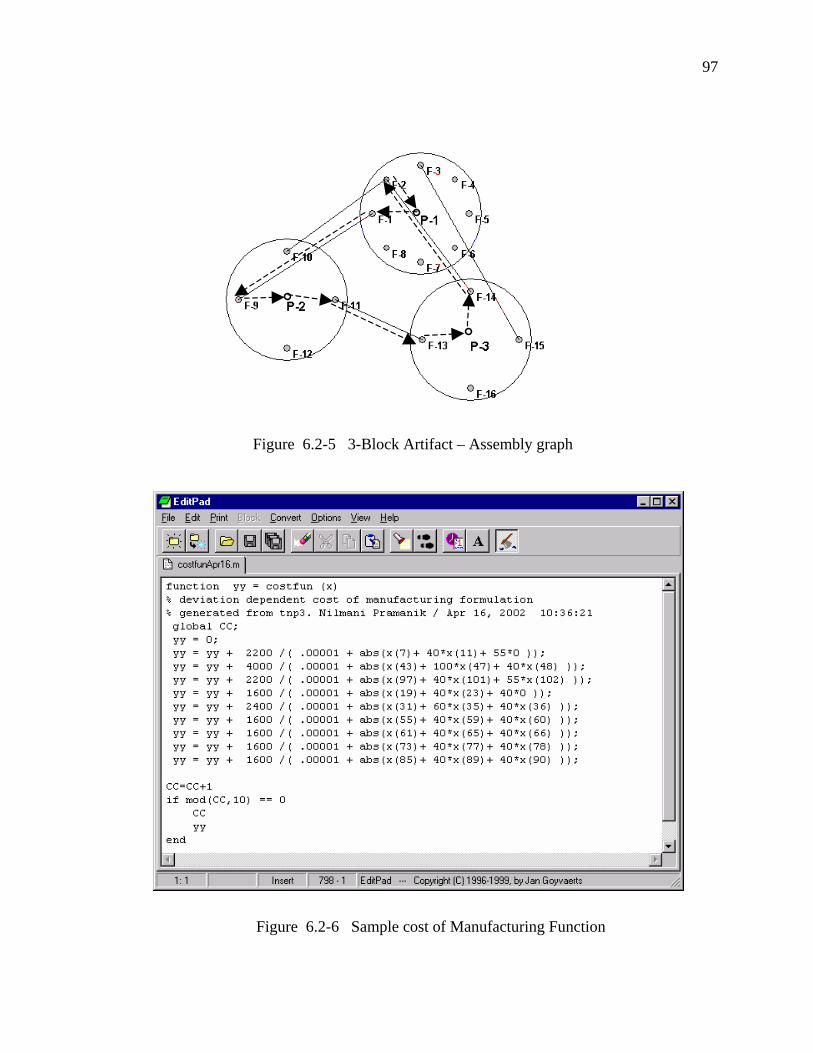
97
Figure 6.2-6 Sample cost of Manufacturing Function
Figure 6.2-5 3-Block Artifact – Assembly graph

98
Figure 6.2-7 Deviation imposed on nominal shape
Table 6.2-1 Optimal deviation parameters

99
Table 6.2-2 Tolerance values mapped from optimal deviation parameters
Figure 6.2-8 Computed tolerance parameters for Part #1

100
6.3 Example Tolerance Synthesis of a Planetary Gearbox
In this example, a typical planetary gearbox (figure 6.3-1) has been used to carry out the
tolerance synthesis operation. Although operations of the tolerance synthesis module for
both the examples are similar, this model has following additional features:
a) This model is more complex with planar and cylindrical features
b) It has more elements and complex connectivity
c) It corresponds to a real-world gearbox
Figure 6.3-1 A Planetary Gearbox
An exploded view of the gearbox is shown in figure 6.3-2. The gearbox has been
modeled as a 5-part system (figure 6.3-3). In order to carry out the tolerance synthesis
work, a detailed model suitable for input to the tolerance synthesis software is first
developed. In this case, the gearbox has been modeled using two feature elements:
cylindrical feature and circular planar features. The model presented here is a simplified
one (the bearings have been eliminated and mating between gear teeth is represented as a
line contact between two cylindrical features at the pitch circle). The gearbox has been

101
represented using five distinct parts. Numbered nodes are used to identify points on the
features where suitable deviation parameters are defined to represent the variation of the
feature. The nominal dimensions of the gearbox parts have been taken from a real model.
However, the synthesis method and applicability is not dependent on specific dimensions.
Figure 6.3-2 Exploded view of the gearbox
Figure 6.3-3 Gearbox modeled as a 5-part system
Input Shaft Output shaft Output Housing with Sun Gear Ring Gear with Planetary Gears Output Housing

102
A typical mating between two parts have been shown in figure 6.3-4 and the assembly graph is
shown in figure 6.3-5
Figure 6.3-4. Mating of output housing with output shaft and ring gear
Figure 6.3-5 Assembly graph (connectivity diagram) of the gearbox

103
The assemblability constraints have been generated using the standard procedure
elaborated earlier. The cost of manufacturing formulation is detailed below for the
specific features.
The cost of manufacturing is computed as a function of the deviation parameters.
Deviation parameters are used to compute a maximum deviation from the nominal
position by taking the extreme points of a virtual condition boundary (VCB). The VCB is
constructed taking into account the datum reference frames and the material condition
modifiers (MMC/LMC/RFC).
For the circular planar features used in this example (figure-6.3-3, nodes: 3, 5, 8, 14, 16,
20, 23 and 25), net deviation of the displaced plane from the nominal position (figure-
6.3-6, node 5) is computed using the results of section 5.7.2.2:
)( 22zyx R θθδδ ++=
where R is the outer radius of the circular planar disc. This δ is used to compute the cost
of manufacturing using the procedure detailed in 5.3.2 as:
))((
)(22
0
22
zyx
PPlanar
R
rRKCθθδε
π
+++
−=
where, KP is a process-dependent proportionality constant, the absolute value of which
can be established by fitting experimental data. For our purpose of using in this example
KP=1 has been assumed. ε0 is an arbitrary small parameter that has been used to eliminate
singularity at zero deviation.

104
For cylindrical features, using the expression for deviation of an arbitrary point on the
surface of the feature (Appendix 7), we can arrive at the maximum deviation for the
cylindrical feature as,
⎟⎠⎞⎜
⎝⎛ +−++++= 2222
max )()(,max yxxyyxr LL δθδθδδδδ
where L is the length of the cylinder.
Using above δmax, the cost function is computed as:
where, KP is the proportionality constant as described for the planar case. For this
example, KP = 1 has been assumed. ε0 is a small parameter used to eliminate singularity
at zero deviation/tolerance and δr is the independent radial deviation of the cylindrical
element.
Based on the above cost functions, the total cost for the entire product is computed as
sum of these cost functions for all the features. The generated cost function as Matlab file
is listed below:
function yy = costfun (x) % deviation dependent cost of manufacturing formulation % generated from tnp3. Nilmani Pramanik / Nov 26, 2002 14:43:50 global CC; yy = 0; yy = yy + 1600.90 /( .001 + max((x(10)^2 + x(11)^2)^0.5,(( x(10) +17.83 * x(8) )^2 + ( x(11) + 17.83 * x(7) )^2)^0.5 )); yy = yy + 823.32 /( .001 + abs(x(16)+(x(14)^2 + 21.60 * x(15)^2 )^0.5 )); yy = yy + 1423.01 /( .001 + max((x(22)^2 + x(23)^2)^0.5,(( x(22) +10.49 * x(20) )^2 + ( x(23) + 10.49 * x(19) )^2)^0.5 )); yy = yy + 1103.96 /( .001 + abs(x(28)+(x(26)^2 + 28.60 * x(27)^2 )^0.5 )); yy = yy + 1600.90 /( .001 + max((x(40)^2 + x(41)^2)^0.5,(( x(40) +17.83 * x(38) )^2 + ( x(41) + 17.83 * x(37) )^2)^0.5 )); yy = yy + 823.32 /( .001 + abs(x(46)+(x(44)^2 + 21.60 * x(45)^2 )^0.5 )); yy = yy + 1423.01 /( .001 + max((x(52)^2 + x(53)^2)^0.5,(( x(52) +10.49 * x(50) )^2 + ( x(53) + 10.49 * x(49) )^2)^0.5 )); yy = yy + 405.37 /( .001 + max((x(58)^2 + x(59)^2)^0.5,(( x(58) +12.70 * x(56) )^2 + ( x(59) + 12.70 * x(55) )^2)^0.5 ));
( )2 2 2 20
2
max , ( ) ( )P
Cylindrical
r x y y x x y
K rLCL L
π
ε δ δ δ θ δ θ δ=
+ + + + + − +

105
yy = yy + 938.71 /( .001 + max((x(64)^2 + x(65)^2)^0.5,(( x(64) +12.70 * x(62) )^2 + ( x(65) + 12.70 * x(61) )^2)^0.5 )); yy = yy + 3623.63 /( .001 + max((x(70)^2 + x(71)^2)^0.5,(( x(70) +12.70 * x(68) )^2 + ( x(71) + 12.70 * x(67) )^2)^0.5) ); yy = yy + 1103.96 /( .001 + abs(x(82)+(x(80)^2 + 28.60 * x(81)^2 )^0.5 )); yy = yy + 2067.37 /( .001 + max((x(88)^2 + x(89)^2)^0.5,(( x(88) +15.24 * x(86) )^2 + ( x(89) + 15.24 * x(85) )^2)^0.5 )); yy = yy + 1103.96 /( .001 + abs(x(94)+(x(92)^2 + 28.60 * x(93)^2 )^0.5 )); yy = yy + 1216.10 /( .001 + max((x(106)^2 + x(107)^2)^0.5,(( x(106) +15.24 * x(104) )^2 + ( x(107) + 15.24 * x(103) )^2)^0.5 )); yy = yy + 1853.20 /( .001 + max((x(112)^2 + x(113)^2)^0.5,(( x(112) +28.58 * x(110) )^2 + ( x(113) + 28.58 * x(109) )^2)^0.5 )); yy = yy + 137.22 /( .001 + abs(x(118)+(x(116)^2 + 10.30 * x(117)^2 )^0.5 )); yy = yy + 277.38 /( .001 + max((x(124)^2 + x(125)^2)^0.5,(( x(124) +5.56 * x(122) )^2 + ( x(125) + 5.56 * x(121) )^2)^0.5 )); yy = yy + 2236.41 /( .001 + abs(x(136)+(x(134)^2 + 28.60 * x(135)^2 )^0.5 )); yy = yy + 1853.20 /( .001 + max((x(142)^2 + x(143)^2)^0.5,(( x(142) +28.58 * x(140) )^2 + ( x(143) + 28.58 * x(139) )^2)^0.5 )); yy = yy + 137.22 /( .001 + abs(0+(x(146)^2 + 10.30 * x(147)^2 )^0.5 )); yy = yy + 277.38 /( .001 + max((x(154)^2 + x(155)^2)^0.5,(( x(154) +5.56 * x(152) )^2 + ( x(155) + 5.56 * x(151) )^2)^0.5 )); CC=CC+1; if mod(CC,100) == 0 CC yy end
This gearbox optimization problem (with the 5-part configuration) has 306 deviation
parameters (variables), 672 linear equality constraints and an 18-component non-linear
cost function. A typical Matlab execution (minimization run) for this example on a 1GHz
Dell OptiPlex GX110 system with 256MB RAM takes about 25 minutes.
The optimization run as described above produces a set of optimal deviation parameters.
These parameters, however, do not have any one-to-one equivalence with standard
tolerance specification as per ANSI Y14.5 and hence these deviation parameters could
not be used directly for arriving at tolerance values. However, it has been shown [Wang
(2003)] that these deviation parameters could be mapped to traditional tolerance
parameters as per ANSI Y14.5. Thus we need to transform the optimal deviation values
to suitable tolerance values or tolerance zones in terms of the traditional tolerance
specifications. In order to do this we need two steps:

106
a) Decide tolerance types that could be assigned/prescribed for individual features,
and
b) Use the deviation-to-tolerance mapping relations to generate a series of
inequalities connecting the tolerance parameters.
The last step b) generates the tolerance zones for each feature. In our example we have
two different types of features: circular planar feature and cylindrical feature and the
deviation to tolerance mapping relations for these two cases are given here from [Wang
(2003)]. For example, for circular planar feature of the output housing (figure 6.3-6, node
5), the mapping relations are:
TL ≤ (∆z - R√( ∆θx2
+∆θy2) ) and (∆z + R√( ∆θx
2 +∆θy
2) ) ≤ TU , where (0, 0, ∆z, ∆θx,
∆θy, 0) are deviation parameters and (TU, TL) are the tolerance parameters.
Figure 6.3-6 Circular planar feature with tolerance parameters TU and TL.
Similarly for the inner cylindrical feature (figure 6.3-3, node 4) of the outer housing, we
can derive following relationships:

107
TUdrTL )2
()(
22≤≤−
−≥
∆+∆
∆∆−∆∆±
TpTUxydr
yx
xy
θθ
θθ
When the solved optimal deviation parameters are put in these inequalities, they generate
a set of linear inequalities. These inequalities define a tolerance zone for that feature in
the (TU TL Tp) space. In this example, tolerance zones for each feature are computed
(tables 6.3-1 and 6.3-2) by taking tolerance types from the possible tolerances that could
be prescribed for these features. Since the deviation to tolerance mapping is one-to-many,
we have to select one possible (suitable) tolerance type
Table 6.3-1 Tolerance zones/values for cylindrical features
The last two columns of Table 6.3-1 shows the computed values of the limits for the right
hand side of the deviation-to-tolerance parameter mapping relations for the cylindrical
features. This gives the possible range of the values TU, TL and Tp constrained by the
Part Feature Outer Cylinder fMin fMax1 Output Housing Radius Length
Feature node 2 14.29 17.83 -0.10 0.10Feature node 3 21.59 10.49 -0.14 0.14
2 Output Shaft Feature node 5 14.29 17.83 -0.02 0.02 Feature node 7 21.59 10.49 -0.14 0.143 Ring Gear
Feature node 15 21.59 15.24 -0.13 0.134 Input Shaft and Sun Gear
Feature node 18 12.70 15.24 -0.14 0.14Feature node 19 10.32 28.58 -0.14 0.14Feature node 21 7.94 6.35 -0.14 0.14
5 Input HousingFeature node 24 10.32 28.58 -0.14 0.14Feature node 26 7.94 6.35 -0.14 0.14
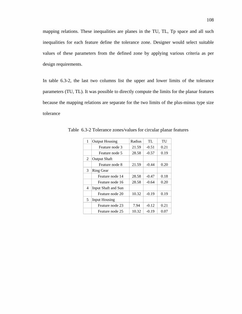
108
mapping relations. These inequalities are planes in the TU, TL, Tp space and all such
inequalities for each feature define the tolerance zone. Designer would select suitable
values of these parameters from the defined zone by applying various criteria as per
design requirements.
In table 6.3-2, the last two columns list the upper and lower limits of the tolerance
parameters (TU, TL). It was possible to directly compute the limits for the planar features
because the mapping relations are separate for the two limits of the plus-minus type size
tolerance
Table 6.3-2 Tolerance zones/values for circular planar features
1 Output Housing Radius TL TUFeature node 3 21.59 -0.51 0.21Feature node 5 28.58 -0.57 0.19
2 Output ShaftFeature node 8 21.59 -0.44 0.20
3 Ring GearFeature node 14 28.58 -0.47 0.18Feature node 16 28.58 -0.64 0.20
4 Input Shaft and SunFeature node 20 10.32 -0.19 0.19
5 Input HousingFeature node 23 7.94 -0.12 0.21Feature node 25 10.32 -0.19 0.07

109
How beautiful it is to do nothing, and then rest afterward.
– Spanish Proverb
Chapter 7
Conclusion
The objective of this research has been to develop a generic object-oriented framework
that could be used as a common platform for design of products both in the conceptual
design stage as well as in detailed design. In the conceptual design stage, a procedure for
converting the product specification/functional requirements into a physical form
(function-to-form mapping) using transformation of product specifications along with
variation of internal parameters of artifacts in a multi-stage design evolution has been
presented. In the detailed design phase, the focus has been on the development of a
generic scheme for the synthesis of tolerances for manufactured parts and in this
endeavor, a scheme for tolerance synthesis has been presented based on minimization of
manufacturing cost subject to assemblability constraints and constraints due to functional
requirements. The proposed schemes have been implemented and example problems
have been solved to establish effectiveness of the schemes.
7.1 Contribution
The following are the contributions of this thesis:
i) A new approach for design synthesis / design evolution has been presented which
operates on a knowledge-based artifact library search and variation of internal

110
parameters of the artifact for selection of best candidate at intermediate stages of
the design evolution.
ii) A new scheme for synthesis of tolerances has been presented which is formulated
as a non-linear constrained optimization (cost minimization) scheme. It is based
on a generic deviation-based formulation.
iii) A new deviation-based cost of manufacturing model has been presented which
can represent the cost of manufacturing as a multi-variate function of deviation
parameters that could be mapped to the tolerance specifications as per ASME
Y14.5M standard.
iv) A new scheme for mapping the generic deviation parameters of features from the
deviation space to tolerance space (tolerance zone) has been introduced.
7.2 Future Work
Major issues of the proposed work have been completed, however, there are some open
issues that could be pursued further for extending the work. These are as listed below:
i) It has been assumed that a product specification is available in a structured format
for carrying out the design synthesis process. However, in general customers’
requirements are generally presented in the form of verbose natural languages. It
would be worth exploring if suitable natural language processing modules
(Natural Language Modeling) could be used to automatically generate tokens that
could be directly used as product specification in standardized form. There are
some works available for converting specifications from natural languages to

111
<attribute, value> tokens. This aspect could be pursued further so that a
generalized routine could be added as a preprocessor to the design synthesis
process.
ii) In the design synthesis, a sample artifact library has been created for a particular
design domain. The library could be extended to encompass widely varying
domain-specific artifacts and knowledge base to ascertain the versatility of the
design evolution process.
iii) The mapping of deviation-to-tolerance has been completed for rectangular-planar,
circular-planar, cylindrical, spherical and conical features. Further work is needed
to develop mapping relations for remaining regular shapes like toroidal, helical
screw, and sculptured features to bring the mapping task to a closure. However,
due to complex non-linear nature of the relationship between the deviation
parameters and the features surface geometry, it may not be possible to generate
the mapping relations in compact form.
iv) The tolerance synthesis method generates constrained non-linear optimization
problem. There is no known theoretical method to ascertain if a global minimum
exists or not. Traditional methods used for solving the problem may not be a
global solution and evolutionary algorithms could be used to explore for
improving the search for global.
v) The advantage that is inherent due to the linear form (KX=B) of the
assemblability constraints, gets somewhat reduced because of the large number of
equations (six for each path or loop in 3-dimensional artifacts) and it would be

112
worth exploring if suitable tools could be developed to eliminate non-critical
constraints from these equations prior to the optimization or after some initial
passes of the optimization run.
vi) For practical use of the new deviation-based cost of manufacturing model,
extensive experimental data needs to be collected and correlated to establish the
constants of the cost of manufacturing formulation for various manufacturing
methods. The author plans to continue this task so that standardized results could
be made available to the designers.
vii) Even though the cost model is generic, only cost of manufacturing has been
formulated. It would be worth exploring to introduce generic deviation-based cost
functions for other costs, like assembly process cost, cost of inspection, cost of
maintenance/repair, etc.
viii) The tolerance synthesis model has been implemented and preliminary studies
have been carried out to link these modules with commercial CAD packages. It
would be worth exploring further as to how this module could dynamically
interact with CAD packages to give the designer a more versatile design
environment.
ix) Convergence criteria for the proposed design synthesis process and complexity of
the proposed algorithms needs evaluation for various artifact configurations in
different design domains.
x) A generic criteria for assemblability of toleranced parts could be studied by
considering the property of a set formed by the intersection of three polytopes
representing: a) assemblability constraints, b) constraints for satisfying the

113
functional requirements and c) tolerancing constraints (tolerance to deviation
mappings). It would depend on whether the constraints indicated in b) and c),
could be converted to polytopes (set of linear inequalities) in the deviation space.
■

114
Appendices
Appendix –1 Class diagrams for various classes
Figure A1.1 Artifact class diagram

115
Figure A1.2 Function Class
Figure A1.3 Behavior Class

116
Figure A1.4 Material Data Class
Figure A1.5 Feature Class

117
Figure A1.6 Tolerance CLass
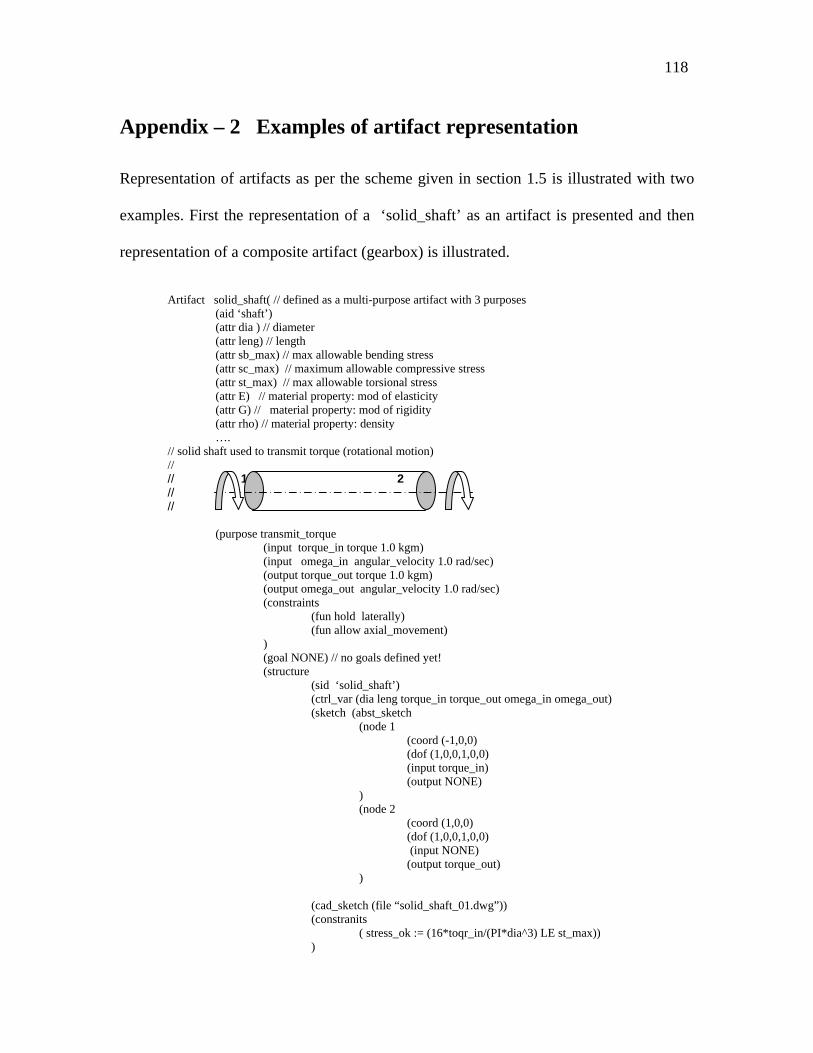
118
Appendix – 2 Examples of artifact representation
Representation of artifacts as per the scheme given in section 1.5 is illustrated with two
examples. First the representation of a ‘solid_shaft’ as an artifact is presented and then
representation of a composite artifact (gearbox) is illustrated.
Artifact solid_shaft( // defined as a multi-purpose artifact with 3 purposes
(aid ‘shaft’) (attr dia ) // diameter (attr leng) // length (attr sb_max) // max allowable bending stress (attr sc_max) // maximum allowable compressive stress (attr st_max) // max allowable torsional stress (attr E) // material property: mod of elasticity (attr G) // material property: mod of rigidity (attr rho) // material property: density ….
// solid shaft used to transmit torque (rotational motion) // // 1 2 // //
(purpose transmit_torque (input torque_in torque 1.0 kgm) (input omega_in angular_velocity 1.0 rad/sec) (output torque_out torque 1.0 kgm) (output omega_out angular_velocity 1.0 rad/sec) (constraints (fun hold laterally) (fun allow axial_movement) ) (goal NONE) // no goals defined yet! (structure (sid ‘solid_shaft’)
(ctrl_var (dia leng torque_in torque_out omega_in omega_out) (sketch (abst_sketch
(node 1 (coord (-1,0,0) (dof (1,0,0,1,0,0) (input torque_in) (output NONE)
) (node 2
(coord (1,0,0) (dof (1,0,0,1,0,0) (input NONE) (output torque_out)
) (cad_sketch (file “solid_shaft_01.dwg”)) (constranits ( stress_ok := (16*toqr_in/(PI*dia^3) LE st_max)) )
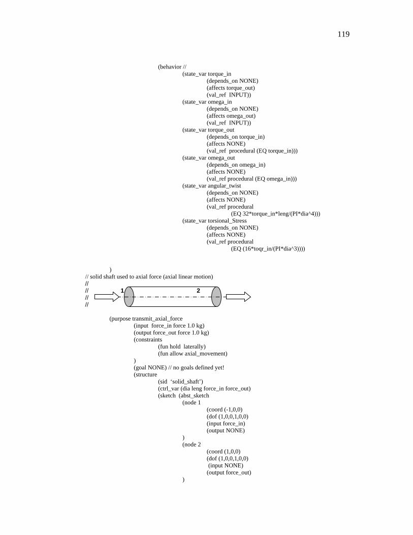
119
(behavior // (state_var torque_in (depends_on NONE) (affects torque_out) (val_ref INPUT)) (state_var omega_in (depends_on NONE) (affects omega_out) (val_ref INPUT)) (state_var torque_out (depends_on torque_in) (affects NONE) (val_ref procedural (EQ torque_in))) (state_var omega_out (depends_on omega_in) (affects NONE) (val_ref procedural (EQ omega_in))) (state_var angular_twist (depends_on NONE) (affects NONE) (val_ref procedural
(EQ 32*torque_in*leng/(PI*dia^4))) (state_var torsional_Stress (depends_on NONE) (affects NONE) (val_ref procedural
(EQ (16*toqr_in/(PI*dia^3))))
)
// solid shaft used to axial force (axial linear motion) // // 1 2 // //
(purpose transmit_axial_force (input force_in force 1.0 kg) (output force_out force 1.0 kg) (constraints (fun hold laterally) (fun allow axial_movement) ) (goal NONE) // no goals defined yet! (structure (sid ‘solid_shaft’)
(ctrl_var (dia leng force_in force_out) (sketch (abst_sketch
(node 1 (coord (-1,0,0) (dof (1,0,0,1,0,0) (input force_in) (output NONE)
) (node 2
(coord (1,0,0) (dof (1,0,0,1,0,0) (input NONE) (output force_out)
)
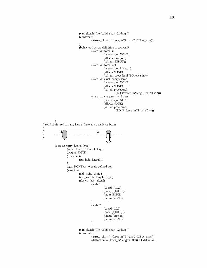
120
(cad_sketch (file “solid_shaft_01.dwg”)) (constranits ( stress_ok := (4*force_in/(PI*dia^2) LE sc_max)) )
(behavior // as per definition in section 5 (state_var force_in (depends_on NONE) (affects force_out) (val_ref INPUT)) (state_var force_out (depends_on force_in) (affects NONE) (val_ref procedural (EQ force_in))) (state_var axial_compression (depends_on NONE) (affects NONE) (val_ref procedural
(EQ 4*force_in*leng/(E*PI*dia^2))) (state_var compressive_Stress (depends_on NONE) (affects NONE) (val_ref procedural
(EQ (4*force_in/(PI*dia^2)))))
)
// solid shaft used to carry lateral force as a cantelever beam // // 1 2 // //
(purpose carry_lateral_load (input force_in force 1.0 kg) (output NONE) (constraints (fun hold laterally) ) (goal NONE) // no goals defined yet! (structure (sid ‘solid_shaft’)
(ctrl_var (dia leng force_in) (sketch (abst_sketch
(node 1 (coord (-1,0,0) (dof (0,0,0,0,0,0) (input NONE) (output NONE)
) (node 2
(coord (1,0,0) (dof (0,1,0,0,0,0) (input force_in) (output NONE)
) (cad_sketch (file “solid_shaft_02.dwg”)) (constranits ( stress_ok := (4*force_in/(PI*dia^2) LE sc_max)) (deflection := (force_in*leng^3/(3EI)) LT deltamax)

121
)
(behavior // as per definition in section 5 (state_var force_in (depends_on NONE) (affects NONE) (val_ref INPUT)) (state_var laterall_deflection (depends_on NONE) (affects NONE) (val_ref procedural
(EQ force_in*leng^3/(3EI)))) (state_var bending_Stress (depends_on NONE) (affects NONE) (val_ref procedural
(EQ (32*force_in*leng/(PI*dia^3))))) )
The behavior of the shaft shown in the three cases can be represented as a method in object-oriented definition. For example, the behavior of in the first case would be represented by following method:
void behavior (double torque_in, double omega_in) { // computes behavioral parameters at time ‘t’ of the shaft for specified torque and // angular velocity.
torque_out = torque_in ; omega_out = omega_in; angular_twist = 32*torque_in*leng/(PI*dia^4); torsional_stress = 16*toqr_in/(PI*dia^3) power = torque_in*omega_in // power transmitted by the shaft }
Above example was for a primitive artifact with single component. We will now consider a ‘gear box’ as a composite artifact with two primitive ‘gear’ artifacts. Before defining the ‘gear box’, we first define a ‘gear’ as follows: // // // // // // // // // // // Artifact gear (
(aid gear) (attr shaft_dia ) // diameter (attr width) // length (attr pitch_dia) // pitch diameter (attr n_teeth) // number of teeth (attr sb_max) // max allowable bending stress (attr sc_max) // maximum allowable compressive stress (attr st_max) // max allowable torsional stress (attr E) // material property: mod of elasticity (attr G) // material property: mod of rigidity (attr rho) // material property: density ….

122
(purpose transmit_torque) (purpose transmit_rotation) (purpose change_speed) (requires (art shaft)) (requires (art key)) (requires (art housing)) (input torque_in torque 1.0 kgm) (input omega_in angular_velocity 1.0 rad/sec) (output torque_out torque 1.0 kgm) (output omega_out angular_velocity 1.0 rad/sec) (constraints (goal NONE) // no goals defined yet! (structure (sid spur_gear’)
(ctrl_var (dia leng torque_in torque_out omega_in omega_out) (sketch (abst_sketch
(node 1 (point)
(coord (0,0,0) // center of gear (dof (0,0,0,1,0,0) (input omega_in) (output NONE)
) (node 2 (circle) // pitch circle
(center (coord (0,0,0)) (dia pitch_dia) (input NONE) (output torque_out) (output omega_out)
) (node 3 (circle) // outer circle
(center (coord (0,0,0)) (dia outer_dia) (input NONE) (output NONEt)
) (cad_sketch (file “spur_gear_01.dwg”)) (constranits ( stress_ok := <contact stress <= allowable stress>)) )
(behavior // as per definition in section 5 (state_var torque_in (depends_on NONE) (affects torque_out) (val_ref INPUT)) (state_var omega_in (depends_on NONE) (affects omega_out) (val_ref INPUT)) (state_var torque_out (depends_on torque_in) (affects NONE) (val_ref procedural (EQ torque_in))) (state_var omega_out (depends_on omega_in) (affects NONE)

123
(val_ref procedural (EQ omega_in))) (state_var angular_twist (depends_on NONE) (affects NONE) (val_ref procedural
(EQ <appropriate eqn>))) (state_var torsional_Stress (depends_on NONE) (affects NONE) (val_ref procedural
(EQ (<appropriate eqn>)))
)
Now we define the artifact ‘gear_box’ to change rotational speed: // // // // // // // // // // // // // // Artifact gear_box (
(aid gear_box) (attr shaft_dia_in ) // input gear diameter (attr shaft_dia_out ) // output gear diameter (attr pitch_dia_in) // input gear pitch diameter (attr n_teeth_in) // number of teeth input gear (attr n_teeth_out) // number of teeth output gear (attr trans_ratio) // speed ration (output_speed/input_speed) // EQ n_teeth_in/n_teeth_out (attr sb_max) // max allowable bending stress (attr sc_max) // maximum allowable compressive stress (attr st_max) // max allowable torsional stress (attr E) // material property: mod of elasticity (attr G) // material property: mod of rigidity (attr rho) // material property: density …. (purpose transmit_torque) (purpose change_rotational_speed) (requires
(art gear) (location (coord (node 1))) (orientation (direction_cosine (cx,cy,cz)) ) (requires
(art gear) (location (coord (node 2))
(orientation (direction_cosine (cx,cy,cz)) )

124
(requires
(art shaft) (location (coord (node 1)))
(orientation (direction_cosine (cx,cy,cz)) ) (requires
(art shaft) (location (coord (node 2)))
(orientation (direction_cosine (cx,cy,cz)) ) (requires
(art key) (location (coord (node 4)))
(orientation (direction_cosine (cx,cy,cz)) ) (requires
(art key) (location (coord (node 5)))
(orientation (direction_cosine (cx,cy,cz)) ) (requires
(art housing) (location (coord (node 1)))
(orientation (direction_cosine (cx,cy,cz)) ) (input torque_in torque 1.0 kgm) (input omega_in angular_velocity 1.0 rad/sec) (output torque_out torque 1.0 kgm) (output omega_out angular_velocity 1.0 rad/sec) (constraints // pcd of two gears should meet // others ) (goal NONE) // no goals defined yet! (structure (sid gear_box)
(ctrl_var (torque_in torque_out omega_in omega_out) (sketch (abst_sketch
(node 1 (point)
(coord (0,0,0) // center of gear in-gear (dof (0,0,0,1,0,0) (input omega_in) (output NONE)
) (node 2 (point // contact point on pcd of both
(coord (0,0,0))) (input NONE) (output torque_out) (output omega_out)
) (node 3 (point // center of out-gear
(coord (0,0,0))) (input NONE) (output omega_out) (output torque_out)
) (node 4

125
(point // key hole location
(coord (0,0,0))) (input NONE) (output omega_out) (output torque_out)
) (node 5 (point // key hole location
(coord (0,0,0))) (input NONE) (output omega_out) (output torque_out)
) (cad_sketch (file “spur_gear_01.dwg”)) (constranits ( stress_ok := <contact stress <= allowable stress>)) )
(behavior // of combined gears (state_var torque_in (depends_on NONE) (affects torque_out) (val_ref INPUT)) (state_var omega_in (depends_on NONE) (affects omega_out) (val_ref INPUT)) (state_var torque_out (depends_on torque_in) (affects NONE) (val_ref procedural (EQ torque_in))) (state_var omega_out (depends_on omega_in) (affects NONE) (val_ref procedural
(EQ omega_in*trans_ratio))) (state_var angular_twist (depends_on NONE) (affects NONE) (val_ref procedural
(EQ <appropriate eqn>))) (state_var torsional_Stress (depends_on NONE) (affects NONE) (val_ref procedural
(EQ (<appropriate eqn>))) )

126
Appendix – 3 Artifact Library
Artifact Cam Follower (Lin) Cam Follower(Osc) Rack & Pinion Spur Gear Box id A1 A2 A3 A4
figure ref figure 1-2 figure 1-1 figure 1-4 figure 1-6 Function rotary_to_linear rotary_to_rotary rotary_to_linear rotary_to_rotary
purpose rotary to linear oscilating rotary to rotary oscilatory rotary to linear rotary to rotary type
equivalence Input w_In w_In w_In w_In
category rotary_motion rotary_motion rotary_motion rotary_motion weight 1 1 1 1
unit rpm rpm rpm rpm from val 100 100 100 100
to val 300 300 300 300 Internal Par E (eccentricity) R (range_angle) R (pinion radius) R (speed_ratio)
category - - - - weight 1 1 1 1
unit mm degree - - from val 0 0 ? 0.25
to val ? 60 ? 4 Output x(x_range) w_Out x_vel w_Out
category linear_oscilatory rotary_oscilatory linear_motion rotary_motion weight 1 1 1 1
unit mm cpm mm/sec rpm from val unknown
to val Constraint C0 C0 C0 C0
type relational relational relational relational expression x = 2*E w_out = w_in x_vel=w_in*R w_out = w_in*R
Constraint C1 C1 C1 C1 Type spatial spatial spatial spatial
Expression axis(w_in) _|_ axis(x) axis(w_in) || axis(w_out) axis(w_in) _|_ dir(x_vel) axis(w_in) || axis(w_out) Artifact Ref cam cam rack spur_gear Artifact Ref follower follower pinion spur_gear Behavior x(t)=2*E*cos(w_in*t) w_out(t)=w_in(t) x_vel(t)=w_in(t)*R w_out(t)=w_in(t)*R

127
Artifact 4-Bar Linkage Belt Pulley Bevel Gear Box Nut & Bolt id A5 A6 A7 A8
figure ref - - figure 1-5 figure 1-3 Function rotary_to_rotary rotary_to_rotary rotary_to_rotary rotary_to_linear
purpose to trasmit rotary motion rotary to rotary rotary to rotary motion rotary to linear type
equivalence Input w_In w_In w_In w_In
category rotary_motion rotary_motion rotary_motion rotary_motion weight 1 1 1 1
unit rpm rpm rpm rpm from val 100 100 100 100
to val 300 300 300 300 Internal Par Lengths of the bars R(speed_ratio) R(speed_ratio) P (pitch)
category - - - - weight 1 1 1 1
unit mm - - mm from val ? 0.5 0.25 1
to val ? 2 4 5 Output w_Out w_Out w_Out x_vel
category rotary_motion rotary_motion rotary_motion linear_motion weight 1 1 1 1
unit rpm rpm rpm mm/sec from val
to val Constraint C0 C0 C0 C0
type relational relational relational relational expression w_out = w_in*R w_out = w_in*R w_out = w_in*R x_vel = w_in*P
Constraint C1 C1 C1 C1 type spatial spatial spatial spatial
expression axis(w_in) || axis(w_out) axis(w_in) || axis(w_out) axis(w_in) _|_ axis(w_out) axis(w_in) || dir(x_vel) Artifact Ref spur_gear belt bevel_gear nut Artifact Ref spur_gear pulley, pulley bevel_gear bolt Behavior w_out(t)=w_in(t)*R w_out(t)=w_in(t)*R w_out(t)=w_in(t)*R x_vel(t)=w_in(t)*P
Note: This table is a simplified version of the actual artifact representation as objects. Only the basic features required to follow the design synthesis example given in this paper have been shown here.

128
Nut Bolt
Rack
Pinion
Cam and Follower (Oscillating) Cam and Follower (Linear) Nut and Bolt Rack and Pinion
Bevel Gear Box Spur Gear Box
Pivot
lever
Driving Shaft
Cam
Cam
Follower
Key

129
Appendix – 4 Interval Arithmetic
The interval arithmetic that would be required to deal with ranges of values for attributes
are elaborated below. In general, we will consider the range from evaluating an
expression as the smallest closed interval including all values of the expression, wherever
is defined, for any values in the ranges of the variables in the expression. We will
interpret each interval as describing the set of possible values of an incompletely known,
but constant, real number or range that is an attribute of an individual physical system.
Thus, a variable with incompletely known value will be described by a closed interval on
the real line: x = [xlb, xub] = {x ∈ R : xlb ≤ xub}, where xlb is the lower bound and xub the
upper bound of x. We will accept and use ∝ and -∝ as possible upper and lower bound,
respectively, for an interval.
Following arithmetic operations are defined for evaluating expressions on intervals. x, y
are expressions evaluating to intervals x=[ xlb, xub], y=[ xlb, xub]
x + y = [xlb +ylb, xub+yub] x - y = [xlb-yub, xub-ylb] x * y = [xlb*ylb, xub*yub] , (xlb ≥ 0 and ylb ≥0) or (xub ≤0 and yub ≤0) = [xlb*yub, xub*ylb] , xub≤0 and ylb≥0 = [xub*ylb, xlb*yub] , xlb ≥0 and yub ≤0 = [xlb*yub, xub*yub] , xlb ≤0 and xub ≥0 and ylb >=0
= [xub*yub, xlb*ylb] , xlb ≤0 and xub ≥ 0 and yub ≤0 = [ylb*xub, yub*xub] , ylb ≤0 and yub ≥ 0 and xlb ≥ 0 = [yub*xub, ylb*xlb] , ylb ≤0 and yub ≥ 0 and xub ≤0 = [min(xlb*yub, xub*ylb), max(xlb*ylb, xub*yub)] xlb ≤0 and xub ≥ 0 and ylb ≤0 and yub ≥ 0
1 / x = [1/xub, 1/xlb] , xlb >0

130
= [1/xub, ∞] , xlb≥0 = [1/xlb, 1/xub] , xub <0 = [-∞, 1/xlb] , xub≤0 = [-∞,∞] , xlb≤0 and xub ≥0 = [∅] , xlb=xub=0 (undefined)
x / y = x * (1/y) |x| = [xlb, xub] , xlb≥0
= [-xub, -xlb] , xub≤0 = [0, max(xub,-xlb)] otherwise
mean(x) = (|xlb|+|xub|)/2 , a single valued quantity.
Evaluating functions:
For monotonically increasing functions, f ∈ M+, where M+
is the class of monotonically increasing functions, f(x) = [flo(xlb), fup(xub)] and f -1(x) = [fup -1(xlb), flo
-1(xub)]. where flo and fup
are the lower and upper bounds (envelopes) of the function f such that ∀x, flo(x) ≤ f(x) ≤ fup(x).

131
Appendix - 5 Transformation of Torsors
A torsor is a tensor-type representation of small displacements and rotations
(corresponding to the six degrees of freedom associated with a space point on a surface
embedded in R3). If we introduce three small displacements along the three local
principal axes at a point A on a surface, as δ = [δx δy δz]T and three rotations θ = [θx θy
θz ]T then the torsor TA/R at A with reference to a datum R can be represented as: TA/R =
[θA δA ]T = [θx θy θz δx δy δz ]T
Torsors transform according to standard rotation & translation rules of axes. However,
the components are small in comparison to the dimension of the components.
The small-displacement torsor mentioned above is used to represent three types of
deviations associated with mating of components in an assembly. Two torsors associated
with each component and a gap torsor at the mating. The two torsors associated with each
feature are: a displacement torsor and a deviation torsor as shown in figure A5-1. The
displacement torsor is an intrinsic variation torsor, which is specific to the element (as for
example, displacement arising out of the variation of the radius of a cylindrical surface).
The displacement torsor represents the deviation of the real surface from the nominal
surface. The gap torsor between two mating features represents possible geometric
variations between the mating features.

132
In order to add the torsors in a loop to form equations connecting the components of the
torsors, a mechanism would be necessary to transform the torsors defined in local
coordinate systems of the individual components into a global reference frame. Since a
torsor is represented by a 1x6 vector, the transformations required would be 6x6
transformation matrices. The rules for transformation of torsors are described below
Gap
Displacement torsor
Part A
Part B
Nominal Surface
Real Surface
Deviation torsor
Deviation torsor
Displacement torsor
Figure A5-1 Interacting torsors at mating surfaces

133
Figure A5-2 Torsor transformation - shifting axes
A small deviation torsor (SDT) TN defined at a point N in the local coordinate system (x,
y, z) with six components (θx, θy, θz, δx, δy , δz) (where θ denotes rotational and δ
denotes linear components of movements) transforms to (TN)ML (where L denotes local
coordinate system) in the same local coordinate system shifted to a new point M is be
given by:
(TN)ML = (θx, θy, θz, δx + (θy*∆z - θz *∆z), δy + (θz *∆x – θx *∆z), δz + (θx *∆y – θy *∆x)) … (A5-1)
This equation could be written in compact notation as: (TN)ML = DTN where D is the
6x6 transformation matrix given by
⎥⎥⎥⎥⎥⎥⎥
⎦
⎤
⎢⎢⎢⎢⎢⎢⎢
⎣
⎡
∆∆−∆−∆∆∆−
=
100001000010000100000010000001
xyxz
yzD
… (A5-2)
where ∆ =(∆x, ∆y, ∆z)T = (XN-XM, YN -YM, ZN-ZM)T is the vector from point M to N in
global coordinate system (X, Y, Z).
Z M
X
Y
x
y
z
N
x
yz
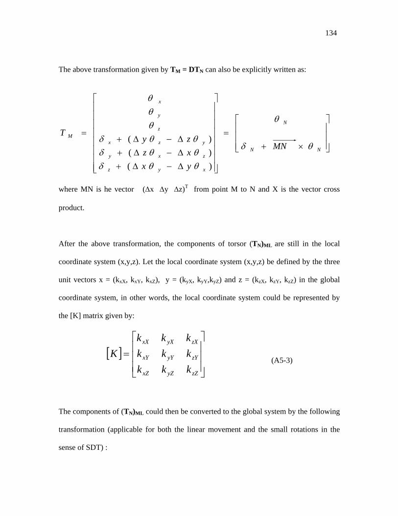
134
The above transformation given by TM = DTN can also be explicitly written as:
⎥⎥⎥
⎦
⎤
⎢⎢⎢
⎣
⎡
×+=
⎥⎥⎥⎥⎥⎥⎥⎥
⎦
⎤
⎢⎢⎢⎢⎢⎢⎢⎢
⎣
⎡
∆−∆+∆−∆+∆−∆+
=
NN
N
xyz
zxy
yzx
z
y
x
M
MN
yxxzzy
Tθδ
θ
θθδθθδθθδ
θθθ
)()()(
where MN is he vector (∆x ∆y ∆z)T from point M to N and X is the vector cross
product.
After the above transformation, the components of torsor (TN)ML are still in the local
coordinate system (x,y,z). Let the local coordinate system (x,y,z) be defined by the three
unit vectors x = (kxX, kxY, kxZ), y = (kyX, kyY,kyZ) and z = (kzX, kzY, kzZ) in the global
coordinate system, in other words, the local coordinate system could be represented by
the [K] matrix given by:
[ ]⎥⎥⎥
⎦
⎤
⎢⎢⎢
⎣
⎡
=
zZyZxZ
zYyYxY
zXyXxX
kkkkkkkkk
K (A5-3)
The components of (TN)ML could then be converted to the global system by the following
transformation (applicable for both the linear movement and the small rotations in the
sense of SDT) :

135
θ X = θx * kxX + θy * kyX + θz * kzX
θY = θx * kxY + θy * kyY + θ z* kzY
θZ = θx * kxZ + θy * kyZ + θz* kzZ
θG = [θ X θ Y θ Z]T = [K][ θx θy θz]T
θG = [K] θ L … (A5-4)
where the subscripts G and L refer to global and local coordinate systems respectively.
δX = [δx + (θy *∆z - θz*∆y)]* kxX + [δy+ (θz*∆x – θx*∆z)]* kyX + [δz+ (θx*∆y – θy *∆x)]* kzX
δY = [δx + (θy *∆z - θz*∆y)]* kxY + [δy+ (θz*∆x – θx*∆z)]* kyY + [δz + (θx*∆y – θy*∆x)]* kzY
δZ = [δx + (θy *∆z - θz*∆y)]* kxZ + [δy+ (θz*∆x – θx*∆z)]* kyZ + [δz + (θx*∆y – θy*∆x)]* kzZ
δG = [δX δY δZ]T = [K] ( [δx δy δz]T + [∆x ∆y ∆z]T × [θ z θ y θ z]T)
where × is the vector cross product.
δG = [K] ( δL + ∆ × θ L ) … (A5-5)
where δL = [δx δy δz]T , ∆ =(∆x, ∆y, ∆z)T, θ L = [ θx θy θz]T
Combining the two transformations, we can write the final result as: (where subscript G
refers to global):
(TN)MG = (θG, δG )
(TN)MG = ([K][ θx θy θz]T , [K] ( [δx δy δz]T + [∆x ∆y ∆z]T × [θ x θ y θ z]T )
… (A5-6)
Above relation could be written as: (TN)MG = K2 (TN)ML … (A5-7)
where K2 is generated using A5-2 and A5-3).

136
Appendix – 6 Example of Generation of Assemblability Constraints
The torsor scheme for the modeling of the small geometric variations of mating features
of an artifact to generate assemblability constraints has been elaborated with a simple
example of a rectangular block (Part-3) enclosed within two channels (Part-1 & Part-2)
(figures A6-1 & A6-2). Apart from the simplified configuration, further simplification
has been done as detailed below so that the relevant transformations and preliminary
computations could be checked manually.
Figure A6-1 Example artifact with three blocks
Loop –6
Loop –5
Loop –4 Loop –3
Loop –2
Loop –1 Part - 1
Part - 2
Part - 3
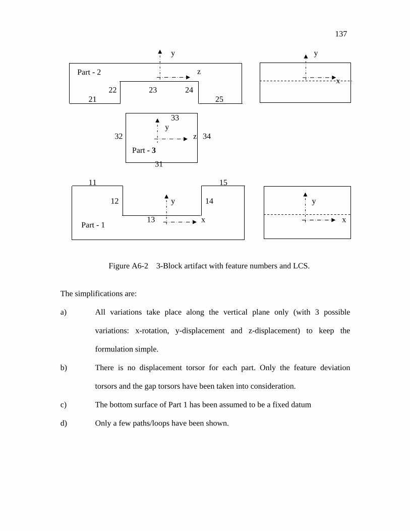
137
Part - 1
Part - 2
y y z x 22 23 24 21 25 33 y 32 z 34 31
11 15 12 y 14 y 13 x x
Figure A6-2 3-Block artifact with feature numbers and LCS.
The simplifications are:
a) All variations take place along the vertical plane only (with 3 possible
variations: x-rotation, y-displacement and z-displacement) to keep the
formulation simple.
b) There is no displacement torsor for each part. Only the feature deviation
torsors and the gap torsors have been taken into consideration.
c) The bottom surface of Part 1 has been assumed to be a fixed datum
d) Only a few paths/loops have been shown.
Part - 3

138
The three parts 1,2, & 3, local axes and contact surfaces have also been shown in the
same sketch. Surfaces have been designated as <part_number><serial_number> such that
surfaces on part 1 are numbered as 11, 12, 13, 14, etc. For generating equations
connecting the variations of the mating surfaces, six loops have been considered.
With the above simplifications, we are left with following configuration: Number of mating surfaces : 14 (all planer) Number of gaps between mating surfaces : 8 Number of surface parameters : 14 x 3 = 42 Number of gap parameters : 8 x 3 = 24 Total number of parameters : 42 + 24 = 66 Number of loops : 6 Number of equations from the loops : 6 x 3 = 18 The six loops are as follows:
Loop-1: 12 32 31 13 Loop-2: 11 21 22 32 32 12 Loop-3: 22 32 33 23 Loop-4: 24 34 33 23 Loop-5: 15 25 24 34 34 14 Loop-6: 14 34 31 13
The associated torsors in their local coordinate systems are: T11 , T12, T13, T14, T15, T21, T22, T23, T24, T25, T31, T32, T33, T34 Typically, each of these torsors would have similar 6-component forms like: T11 = [θ11 δ11 ]T = [θx11 0 0 0 δy11 δz11 ]T , T12 = [θ12 δ12 ]T = [θx12 0 0 0 δy12 δz12 ]T The gap torsors are: G11/21, G12/32, G13/31, G14/34, G15/25, G22/32, G23/33, G24/34 with typical forms given by: G11/21 = [θg11/21 δg11/21 ]T = [θgx11/21 0 0 0 δgy11/21 δgz11/21 ]T

139
We now consider the Loop - 1 (12 32 31 13) and write the torsor equation for the loop as:
T12 + G12/32 + (-T32 ) + T31 + (-G13/31 ) + (-T13 ) = 0 Transforming all the terms in the above equation in Part–1’s frame of reference, the equation becomes, T12
+ (D12/23)12 G12/32 + (D32)12 (-T32 ) +(D31)12 T31 +(D13/31)12 G13/31 + (D13)12 (-T13 ) = 0 where the D’s are the corresponding transformations with respect to the Part - 1. Writing the D’s in full, and carrying out the operations, the above equation becomes,
[θx12 0 0 0 δy12 δz12 ]T + [θgx12/32 0 0 0 δgy12/32 δgz12/32 ]T - [θx32 0 0 0 δy32 + θx32 (z32 - z12) δz32 + θx32 (y32 - y12) ]T + [θx31 0 0 0 δy31 + θx31 (z31 - z12) δz31 + θx31 (y31 - y12) ]T + [θgx13/31 0 0 0 δgy13/31 + θgx13/31 (z31 - z12) δgz13/31 + θgx13/31 (y31 - y12)]T - [θx13 0 0 0 δy13 + θx13 (z13 - z12) δz13 + θx13 (y12 - y12)]T
= [ 0 0 0 0 0 0 ]T
Equating each component to zero gives 6 equations. In this present case there are only 3 equations due to the restricted space of the example.
θx12 + θgx12/32 - θx32 + θx31 + θgx13/31 - θx13 = 0
δy12 + δgy12/32 - δy32 - θx32 (z32 - z12) + δy31 + θx31 (z31 - z12) + δgy13/31 + θgx13/31 (z31 - z12) - δy13 + θx13 (z13 - z12) = 0
δz12 + δgz12/32 - δz32 - θx32 (y32 - y12) + δz31 + θx31 (y31 - y12) + δgz13/31 + θgx13/31 (y31 - y12) - δz13 + θx13 (y12 - y12) = 0
Each of the six loops will give 3 similar equations. Altogether 18 equations would be formed connecting the 66 parameters. Let us repeat the procedure of forming the equations for Loop – 2 (11 21 22 32 32 12) The torsor equation for the Loop - 2 is: T11 + G11/21 + (-T21 ) + T22 + (G22/32 ) + (-T32 ) + T32 + (G32/12 ) + (-T12 ) = 0 i.e. T11 + G11/21 + (-T21 ) + T22 + (G22/32 ) + (G32/12 ) + (-T12 ) = 0

140
Transforming all the terms in the above equation in Part–1’s frame of reference, the equation becomes, T11
+ (D11/21)11 G11/21 + (D21)11 (-T21 ) +(D22)11 T22 +(D22/32)11 G22/32 + + (D32/12)11 G22/12 + (D12)11 (-T12 ) = 0 where the D’s are the corresponding transformations with respect to the Part - 1. Writing the D’s in full, and carrying out the operations, the above equation becomes,
[θx11 0 0 0 δy11 δz11 ]T + [θgx11/21 0 0 0 δgy11/21 δgz11/21 ]T - [θx21 0 0 0 δy21 + θx21 (z21 - z11) δz21 + θx21 (y21 - y11) ]T + [θx22 0 0 0 δy22 + θx22 (z22 - z11) δz22 + θx22 (y22 - y11) ]T + [θgx22/32 0 0 0 δgy22/32 + θgx22/32 (z22 - z11) δgz22/32 + θgx22/32 (y22 - y11)]T + [θgx32/12 0 0 0 δgy32/12 + θgx32/12 (z32 - z11) δgz32/12 + θgx32/12 (y32 - y11)]T - [θx12 0 0 0 δy12 + θx12 (z12 - z11) δz12 + θx12 (y12 - y11)]T
= [ 0 0 0 0 0 0 ]T
Equating each component to zero gives following 3 equations:
θx11 + θgx11/21 - θx21 + θx22 + θgx22/32 + θgx32/12 - θx12 = 0
δy11 + δgy11/21 - δy21 - θx21 (z21 - z11) + δy22 + θx22 (z22 - z11) + δgy22/32 + + θgx22/32 (z22 - z11) +δgy32/12 + θgx32/12 (z32 - z11) - δy12 - θx12 (z12 - z11) = 0
δz11 + δgz11/21 - δz21 - θx21 (y21 - y11) + δz22 + θx22 (y22 - y11) + δgz22/32 + θgx22/32 (y22 - y11) + δgz32/12 + θgx32/12 (y32 - y11) - δz12 - θx12 (y12 - y11) = 0
Similar procedures would yield the rest of the equations for the remaining four loops.

141
Appendix – 7 Mapping of Deviation Parameters to Tolerance Parameters
For completeness, following is included here from [Wang (2003)] on the mapping of
deviation parameters to tolerance zones.
A7.1 Cylindrical Feature - Modified to MMC
A cylindrical feature with a given tolerance specification is taken as shown in Figure
A7.1-1 and the local coordinate system (LCS) for defining the deviation parameters is
shown in Figure A7.1.-2. The VCB of the cylindrical surface is constructed by using the
rules in 3.6.1 and the VCB has the following properties:
• A perfect shape as that of the nominal cylindrical feature
• A size (diameter) of max size plus geometric tolerance, because its external feature
and the positional tolerance is modified to MMC
• A perfect orientation as that of the nominal cylindrical feature (vertical to C)
• A perfect location as that of the nominal cylindrical feature
For the cylindrical surface, the LCS is: z-axis along the axis of the cylinder and (x, y) are
local orthogonal co-ordinates on the middle of the axis. For this surface, the deviation
parameters are: (∆x, ∆y, 0, ∆θx, ∆θy, 0) and dr. Based on this notation, mapping relations
are derived as detailed below. For a point P (r*cosθ, r*sinθ, z), on the nominal
cylindrical surface:
Deviation parameters = (∆x, ∆y, 0, ∆θx, ∆θy, 0)
Tolerance parameters = (TU, TL, TP )
SDT are: Dd = {∆θ ∆d} = {∆θx ∆θy 0 ∆x ∆y 0}T
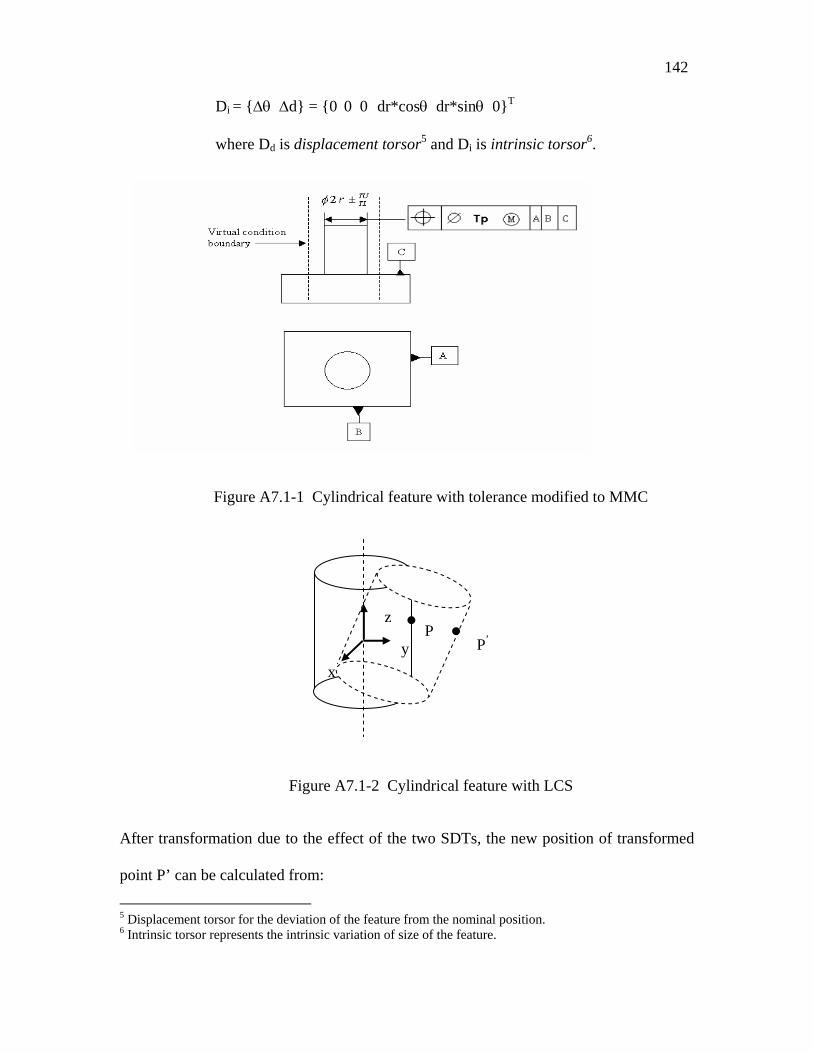
142
Di = {∆θ ∆d} = {0 0 0 dr*cosθ dr*sinθ 0}T
where Dd is displacement torsor5 and Di is intrinsic torsor6.
Figure A7.1-1 Cylindrical feature with tolerance modified to MMC
Figure A7.1-2 Cylindrical feature with LCS
After transformation due to the effect of the two SDTs, the new position of transformed
point P’ can be calculated from:
5 Displacement torsor for the deviation of the feature from the nominal position. 6 Intrinsic torsor represents the intrinsic variation of size of the feature.
P z
yx
P’P

143
⎥⎥⎥⎥
⎦
⎤
⎢⎢⎢⎢
⎣
⎡
+∆++∆−∆+∆−+∆+∆++
=
⎥⎥⎥⎥
⎦
⎤
⎢⎢⎢⎢
⎣
⎡++
⎥⎥⎥⎥
⎦
⎤
⎢⎢⎢⎢
⎣
⎡
∆∆−∆∆−∆∆
1sin)(cos)(
sin)(cos)(
1
sin)(cos)(
100001
1001
θθθθθθθθ
θθ
θθθθ
drrdrrzyzdrrxzdrr
zdrrdrr
yx
xy
x
y
xy
x
y
The 4 by 4 matrix on left hand side of the equation is the transformation matrix for point
P following the assumed transformation sequence ∆x ∆y ∆θx ∆θy by displacement
torsor. The 4 by 1 matrix (vector) on the left hand side of the equation represent the
changed position of point P by intrinsic torsor. Thus the new position P’ is given by
Hence, the constraint equation will be:
4/Tp)TU2r()sin)(()cos)(( 222 ++≤∆+∆−++∆+∆++ yzdrrxzdrr xy θθθθ
where θ ∈ (0, 2π). The left hand side (LHS) is a function of two independent parameters
θ and z. The inequality should be valid for ∀θ ∈ (0, 2π) and ∀z ∈ (0, L). This is done by
finding the maximum of the LHS with respect to θ and z. Writing the LHS of the above
equation as: f(θ,z) = (a*cosθ+b*z+c)2 + (a*sinθ+d*z+e)2, where a = r+dr, b = ∆θy , c =
∆x, d=-∆θx, and e=∆y , and minimizing f with respect to θ and z, the
maximum/minimum value of f is found. After some reduction of the resulting algebraic
expressions using Matlab, the final set of mapping relations are established as:
TUdrTL )2
()(22
≤≤−+
≤+
−±
TpTUbd
cdbedr
)sin)(cos)( , sin)(, cos)(( θθθθθθθθ drrdrrzyzdrrxzdrr xyxy +∆++∆−∆+∆−+∆+∆++

144
and
TUdrTL )2
()(22
≤≤−−
≥+
−±
TpTUbd
cdbedr
for external and internal cylindrical features respectively.
A7.2 Spherical Feature
For the spherical surface, a LCS is defined as: z-axis along radius of the sphere and (x, y)
are local orthogonal co-ordinates at the center of the sphere (Figures A7.2-1 & 2). For
this feature the deviation parameters of the SDT are: (∆x, ∆y, ∆z, 0, 0, 0 ) and dr. Based
on this notation, mapping relations are derived connecting these parameters with the
specified tolerance values as detailed below.
Figure A7.2-1 Spherical feature with LCS
z
yx

145
Figure A7.2-2 Spherical feature with tolerance specification
The VCB of the spherical surface is constructed with the following properties:
• A perfect shape as that of the nominal spherical feature
• A size (diameter) of 2r+TU+Tp, because it’s external feature and the positional
tolerance is modified to MMC
• A perfect location as that of the nominal cylindrical feature
By applying the same procedures as was followed for the cylindrical case, we have:
Dd = {∆θ ∆d} = {0 0 0 ∆x ∆y ∆z}T
Di = {∆θ ∆d} = {0 0 0 dr*sinφ*cos ψ dr*sinφ*sinψ dr*cosφ}T
⎥⎥⎥⎥
⎦
⎤
⎢⎢⎢⎢
⎣
⎡
++∆++∆++∆
=
⎥⎥⎥⎥
⎦
⎤
⎢⎢⎢⎢
⎣
⎡
+++
⎥⎥⎥⎥
⎦
⎤
⎢⎢⎢⎢
⎣
⎡
∆∆∆
1cos)(
sinsin)(cossin)(
1cos)(
sinsin)(cossin)(
1000100010001
ψψφψφ
ψψφψφ
drrzdrrydrrx
drrdrrdrr
zyx

146
The 4 x 4 matrix on the left hand side of the above equation is the transformation matrix
for any point on the spherical surface due to displacement torsor assuming the
transformation sequence ∆x ∆y ∆z. The 4 x 1 matrix (vector) on left hand side of the
equation represents the changed position of the point due to the intrinsic torsor. The
constraints ont eh VCB is expressed as::
4/)2()cos)(()sinsin)(()cossin)((
2
222
TPTUrdrrzdrrydrrx
++≤
++∆+++∆+++∆ ψψφψφ
The above inequality should be valid for ∀Φ ∈ (0, 2π) and ∀Ψ ∈ (0, 2π) and hence the
parameters Φ and Ψ needs to be eliminated by maximizing the following function.
ψψφψφψφψφ cos2sinsin2cossin2cossin),( 22 zyxaaf ∆+∆+∆++=
where a = r + dr
zyxa f yxa f
0sin2cossin2sinsin2sincos20/0)sincossin(cos20/
=∆−∆+∆−−⇒=∂∂=∆+∆+⇒=∂∂
ψψφψφψψψψψφφφ
Here, we have two sets of solutions (Maple V has been used to get the solutions in
symbolic form):
1)
)_2_)2(_2_(
,2
)12(
222222324
1
yyzazxazxyzyazazRootofwhere
zxyatg n
∆−∆+∆+−∆∆+∆+∆+∆−=∆+∆∆−
−=+= −
β
βψπφ

147
2)
)_)222(_)222(_)2
22(_)222((
))12((),)(
)((sin
22222
3222222442222432
234224422224
222222
21
222
22222221
xyazzyzazaxzazazxaxyyaxyazyza
xzazazxyyxyaxaaRootofwhere
zayxaxytg
azayxayzayxax
∆∆+∆−∆∆
−∆−∆∆+∆+∆+∆−∆−∆−∆∆−−+∆∆
+∆∆−∆+∆∆+∆+∆+∆+∆−=
∆−∆−∆+−−∆∆
=∆−∆−∆+−
∆−∆−∆+∆+−∆−= −−
γ
γγγγγψ
γγγγγγγφ
The final set of mapping relations are:
TUdrTL
TpTUrf
≤≤−
++≤ 2
max )2
2(
When toleranced feature is internal, (for example a hole), the relation becomes:
TUdrTL
TpTUrf
≤≤−
−+≥ 2
min )2
2(
If the external feature is modified to LMC, the relations are:
TUdrTL
TpTLrf
≤≤−
−−≥ 2
min )2
2(
If the internal feature is modified to LMC, the relations are:
TUdrTL
TpTLrf
≤≤−
+−≤ 2
max )2
2(
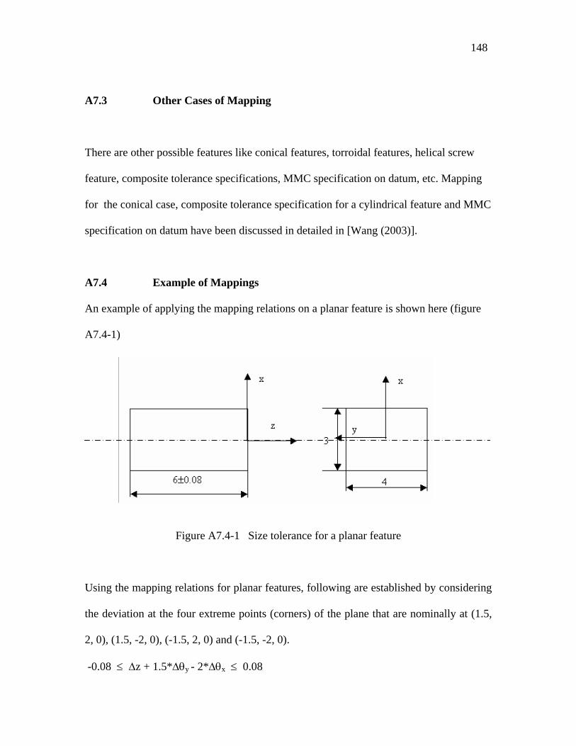
148
A7.3 Other Cases of Mapping
There are other possible features like conical features, torroidal features, helical screw
feature, composite tolerance specifications, MMC specification on datum, etc. Mapping
for the conical case, composite tolerance specification for a cylindrical feature and MMC
specification on datum have been discussed in detailed in [Wang (2003)].
A7.4 Example of Mappings
An example of applying the mapping relations on a planar feature is shown here (figure
A7.4-1)
Figure A7.4-1 Size tolerance for a planar feature
Using the mapping relations for planar features, following are established by considering
the deviation at the four extreme points (corners) of the plane that are nominally at (1.5,
2, 0), (1.5, -2, 0), (-1.5, 2, 0) and (-1.5, -2, 0).
-0.08 ≤ ∆z + 1.5*∆θy - 2*∆θx ≤ 0.08

149
-0.08 ≤ ∆z + 1.5*∆θy + 2*∆θx ≤ 0.08
-0.08 ≤ ∆z – 1.5*∆θy + 2*∆θx ≤ 0.08
-0.08 ≤ ∆z – 1.5*∆θy - 2*∆θx ≤ 0.08
The above inequalities result in a diamond shape in deviation space as shown in figure
A7.4-2.
Figure A7.4-2 Deviation space for size tolerance of a planar feature
∆θx
∆θy
z
0.08
-0.08
0.04
-0.04
0.053 -0.053

150
Appendix – 8 Implementation: Listing of major modules
Program Listing - Main module
Attribute VB_Name = "tnp3Main" 'Option Explicit Global Const maxNodes = 999 Global Const maxParts = 999 Global Const x0StartD = 0.001 ' mm Global Const x0StartR = 0.0001 ' rad Global Const nonSingularEps = 0.00001 Type aArtifact id As String aType As String nextArt As Object End Type Type aGap n As Integer 'node f1 As Integer 'from f2 As Integer 'to End Type Type aTorsor rX(3) As Double dX(3) As Double End Type Type xLink fromArt As Integer fromFeature As Integer gap As Integer ' gap node toArt As Integer toFeature As Integer End Type Type myLoop nLoop As Integer fromArt As Integer fromFeature As Integer gap As Integer ' gap node toArt As Integer toFeature As Integer End Type Type xFeature id As String ' Feature id typ As String 'Feature type ref As Integer ' a reference point, generally the center but could be any other point center As Integer ' node number of the center of the Feature LCS(3, 3) As Double ' x=outward normal, y & z on plane DCs nod(10) As Integer ' nodes to define the feature part As Integer tol As tolerance ' tolerance class isDatum As Boolean Ly As Double 'Ly and Lz are lengths of edges along local Y & Z for rectangles Lz As Double 'Ly and Lz are Outer and inner radii for circular-planar End Type Type parts id As String name As String

151
center As Integer 'center node# LCS(3, 3) As Double ' local x, y & z DCs isTerminal As Boolean Features(9) As Integer End Type Type aNode x(3) As Double 'x,y,z coordinates dof(6) As Integer 'degrees of freedom 1=specifed, 0=unspecified knownDeviation As Boolean tor As aTorsor End Type Type xloop typ As String ' typ= 'P'art, 'F'ace, 'G'ap fromArt As Integer fromFeature As Integer gap As Integer toFeature As Integer toArt As Integer End Type Type xCircle x As Single y As Single r As Single End Type Type kMat i As Integer j As Integer id As String End Type Type Vector x(3) As Double End Type Public getFileOked As Boolean Public dofName(6) As String, nCons As Integer Public xFile, eqStr As String, eqNum As Integer Public x0(maxNodes * 6) As Double 'x0 holds the initial value of X Public b0(maxNodes * 6) As Double 'b0 holds the value of b of KX = b Public nCircle As Boolean Public Circles(99) As xCircle Public nParts As Integer Public nNodes As Integer Public nLinks As Integer Public nFeatures As Integer Public LoopCount As Integer Public nPathElements As Integer Public artNow As String Public aParts(maxParts) As parts Public aNodes(maxNodes) As aNode Public aLink(maxParts) As xLink Public aFeatures(maxNodes) As xFeature Public gap(99) As aGap Public nGaps As Integer Public allPaths() As myLoop Public PathList() As String Public UltoPath() As String Public rootArt As Integer Public partSelected As Integer 'used in drawing loopForm Public tTran(6, 6) As Double ' torsor transformation matrix Public kMat() As Double Public KTree As biTree Public dumpTree2File As String

152
Public dumpFile As Integer Public artWindow As artDraw ' was loopForm Public fMainForm As frmMain Sub Main() Dim fLogin As New frmLogin fLogin.Show vbModal If Not fLogin.OK Then 'Login Failed so exit app End End If Unload fLogin Randomize Set fMainForm = New frmMain Set KTree = New biTree nCircle = False fMainForm.Show End Sub Sub processArt(sFile As String) Dim nF As Integer, sLine As String, sx As String, sY As String Dim j As Integer, k As Integer, tnod As Node, Tokens(20) As String Dim i As Integer, ii As Integer nF = FreeFile j = InStr(sFile, ".") sx = Left(sFile, j - 1) sY = StrReverse(sx) 'Get the artifact name from the file name artNow = UCase(Mid(sx, Len(sx) - InStr(sY, "\") + 2)) Open sFile For Input As #nF 'Input #nf, sLine Line Input #nF, sx 'title of the artifact one line fMainForm.ArtName.Caption = sx fMainForm.Caption = sFile fMainForm.Show ' set up the Artifact tree root Set tnod = fMainForm.ArtTree.Nodes.Add(, , "Root", artNow, 1, 2) tnod.EnsureVisible fMainForm.ArtTree.Visible = True fMainForm.ArtName.Visible = True fMainForm.nodeList.Visible = True 'now get the actual artifact definition data nParts = 0 nNodes = 0 nLinks = 0 nFeatures = 0 fMainForm.nodeList.Clear While Not EOF(nF) Line Input #nF, sLine j = getTokens(sLine, Tokens) sx = Tokens(1) 'first token, the controller Select Case sx Case "PART:" ' part definitions nParts = nParts + 1 j = Val(Tokens(2)) aParts(j).id = "P" + Tokens(2) aParts(j).name = Tokens(3) aParts(j).center = Val(Tokens(4)) aParts(j).isTerminal = Val(Tokens(5)) <> 0 'store the LCS of center of each part For i = 1 To 3 For k = 1 To 3 aParts(j).LCS(k, i) = Val(Tokens(5 + (i - 1) * 3 + k))

153
Next Next Set tnod = fMainForm.ArtTree.Nodes.Add("Root", tvwChild, aParts(j).id, aParts(j).name, 1, 2) tnod.EnsureVisible Case "FEATURE:" 'feature definions nFeatures = nFeatures + 1 i = Val(Tokens(2)) aFeatures(i).id = "F" + Tokens(2) aFeatures(i).typ = Tokens(4) 'if feature type is CYL, then 3 points are reqd. 'p1 , p2 two ends of the axis and f the point where torsor is defined. aFeatures(i).center = Val(Tokens(5)) ' feature center aFeatures(i).ref = Val(Tokens(6)) ' feature reference point for outward normal k = Val(Tokens(3)) 'part number where used aFeatures(i).part = k aParts(k).Features(0) = aParts(k).Features(0) + 1 'one more Feature aParts(k).Features(aParts(k).Features(0)) = i sY = aParts(k).id Set tnod = fMainForm.ArtTree.Nodes.Add(sY, tvwChild, _ sY + aFeatures(i).id, sY + aFeatures(i).id + Tokens(4), 1, 2) tnod.EnsureVisible jj = 0 sY = sY + aFeatures(i).id If Tokens(4) = "PLANE2" Then 'circular-planar feature, get two radii aFeatures(i).Ly = Val(Tokens(7)) aFeatures(i).Lz = Val(Tokens(8)) jj = 2 End If j = j - 6 - jj ' rest of the nodes For ii = 7 + jj To 7 + j + jj - 1 'add the nodes in the tree as well as Featurelist aFeatures(i).nod(0) = aFeatures(i).nod(0) + 1 'increment node count aFeatures(i).nod(aFeatures(i).nod(0)) = Tokens(ii) Set tnod = fMainForm.ArtTree.Nodes.Add(sY, tvwChild, _ sY + "N" + Tokens(ii), "Node:" + Tokens(ii), 3, 4) tnod.EnsureVisible Next Case "LINK:" ' link between part/features nLinks = nLinks + 1 aLink(nLinks).fromArt = aFeatures(Val(Tokens(2))).part aLink(nLinks).fromFeature = Val(Tokens(2)) aLink(nLinks).toFeature = Val(Tokens(3)) aLink(nLinks).gap = Val(Tokens(4)) aLink(nLinks).toArt = aFeatures(Val(Tokens(3))).part ' keep the reverse path as well! nLinks = nLinks + 1 aLink(nLinks).fromArt = aFeatures(Val(Tokens(3))).part aLink(nLinks).fromFeature = Val(Tokens(3)) aLink(nLinks).gap = Val(Tokens(4)) aLink(nLinks).toFeature = Val(Tokens(2)) aLink(nLinks).toArt = aFeatures(Val(Tokens(2))).part 'store the gap definitions nGaps = nGaps + 1 gap(nGaps).n = Val(Tokens(4)) gap(nGaps).f1 = Val(Tokens(2)) gap(nGaps).f2 = Val(Tokens(3)) Case "NODE:" 'nodal data nNodes = nNodes + 1 j = Val(Tokens(2)) aNodes(j).x(1) = Val(Tokens(3)) aNodes(j).x(2) = Val(Tokens(4)) aNodes(j).x(3) = Val(Tokens(5)) ' 'dof(ii)='1' if known/specified disp else 0 For ii = 1 To 6 aNodes(j).dof(ii) = IIf(Trim(Tokens(5 + ii)) = "", 0, 1)

154
Next ' With aNodes(j).tor .rX(1) = Val(Tokens(6)) .rX(2) = Val(Tokens(7)) .rX(3) = Val(Tokens(8)) .dX(1) = Val(Tokens(9)) .dX(2) = Val(Tokens(10)) .dX(3) = Val(Tokens(11)) End With sx = Format(Tokens(2), "0000") + " " For i = 3 To 11 sx = sx + Format(Tokens(i), " 0000.00") Next fMainForm.nodeList.AddItem (sx) Case "MISC:" 'other data - for future use Case "DISP:" 'nodal displacements from prev run/from known sources 'node, rx, ry, rz, dx, dy, dz j = Val(Tokens(2)) For ii = 1 To 6 If aNodes(j).dof(ii) = 1 Then 'known/specified and do nothing Else 'add it If ii < 4 Then ' first 3 rotx aNodes(j).tor.rX(ii) = Val(Tokens(2 + ii)) Else 'last three deltax aNodes(j).tor.dX(ii - 3) = Val(Tokens(2 + ii)) End If End If Next ' Case Else 'for the time being ignore others... End Select Wend ' ' generateLCS ' generate local coordinate system 3 X 3 marix ' for each Feature/features of each part ' 'generate nodal displacements from known values at feature center 'must be called AFTER generateLCS center2Nodes "" ' fMainForm.nodeList.Visible = True fMainForm.NodalButton.Visible = True Close nF End Sub Sub generateLCS() ' Generates LCS of each Feature/feature ' by assuming local X=Outward normal (away from material) ' Y= Vertically up if X is horizontal, else Y= one of the edges ' Z= (X x Y) Dim i, j, k, m, nP, fTyp Dim xLam As Double Dim ve(5) As Vector For nP = 1 To nParts For j = 1 To aParts(nP).Features(0) 'all Features k = aParts(nP).Features(j) fTyp = aFeatures(k).typ If fTyp = "PLANE" Or fTyp = "PLANE2" Then ' ' ve(1)=local-x, ve(2)=local-y, ve(3)=local-z ' ve(0) is the vector from he ref point (generally, center ' of the part) to Feature center ' ve2 = edge 1, ve3=edge 2 ' For m = 1 To 3
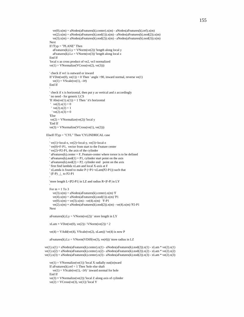
155
ve(0).x(m) = aNodes(aFeatures(k).center).x(m) - aNodes(aFeatures(k).ref).x(m) ve(2).x(m) = aNodes(aFeatures(k).nod(1)).x(m) - aNodes(aFeatures(k).nod(2)).x(m) ve(3).x(m) = aNodes(aFeatures(k).nod(2)).x(m) - aNodes(aFeatures(k).nod(3)).x(m) Next If fTyp = "PLANE" Then aFeatures(k).Ly = VNorm(ve(2)) 'length along local y aFeatures(k).Lz = VNorm(ve(3)) 'length along local z End If 'local x as cross product of ve2, ve3 normalized ve(1) = VNormalize(VCross(ve(2), ve(3))) ' check if ve1 is outward or inward If VDot(ve(0), ve(1)) < 0 Then ' angle >90, inward normal, reverse ve(1) ve(1) = VScale(ve(1), -1#) End If ' ' check if x is horizontal, then put y as vertical and z accordingly ' no need - for generic LCS 'If Abs(ve(1).x(1)) = 1 Then ' it's horizontal ' ve(2).x(1) = 0 ' ve(2).x(2) = 1 ' ve(2).x(3) = 0 'Else ve(2) = VNormalize(ve(2)) 'local y 'End If ve(3) = VNormalize(VCross(ve(1), ve(2))) ElseIf fTyp = "CYL" Then 'CYLINDRICAL case ' ' ve(1)=local-x, ve(2)=local-y, ve(3)=local-z ' ve(0)=F-P1, vector from start to the Feature center ' ve(2)=P2-P1, the axis of the cylinder ' aFeatures(k).center = F, Feature-center where torsor is to be defined ' aFeatures(k).nod(1) = P1, cylinder start point on the axis ' aFeatures(k).nod(2) = P2. cylinder end point on the axis ' first find lambda xLam and local X-axis at F ' xLamda is found to make P (=P1+xLam(P2-P1)) such that ' (F-P) _|_ to P2-P1 ' 'store length L=|P2-P1| in LZ and radius R=|F-P| in LY ' For m = 1 To 3 ve(3).x(m) = aNodes(aFeatures(k).center).x(m) 'F ve(4).x(m) = aNodes(aFeatures(k).nod(1)).x(m) 'P1 ve(0).x(m) = ve(3).x(m) - ve(4).x(m) 'F-P1 ve(2).x(m) = aNodes(aFeatures(k).nod(2)).x(m) - ve(4).x(m) 'P2-P1 Next aFeatures(k).Ly = VNorm(ve(2)) ' store length in LY xLam = VDot(ve(0), ve(2)) / VNorm(ve(2)) ^ 2 ve(4) = VAdd(ve(4), VScale(ve(2), xLam)) 've(4) is now P aFeatures(k).Lz = VNorm(VDiff(ve(3), ve(4))) 'store radius in LZ ve(1).x(1) = aNodes(aFeatures(k).center).x(1) - aNodes(aFeatures(k).nod(2)).x(1) - xLam * ve(2).x(1) ve(1).x(2) = aNodes(aFeatures(k).center).x(2) - aNodes(aFeatures(k).nod(2)).x(2) - xLam * ve(2).x(2) ve(1).x(3) = aNodes(aFeatures(k).center).x(3) - aNodes(aFeatures(k).nod(2)).x(3) - xLam * ve(2).x(3) ve(1) = VNormalize(ve(1)) 'local X radially out(in)ward If aFeatures(k).ref = 1 Then 'hole else shaft ve(1) = VScale(ve(1), -1#) ' inward normal for hole End If ve(3) = VNormalize(ve(2)) 'local Z along axis of cylinder ve(2) = VCross(ve(3), ve(1)) 'local Y

156
End If 'Now store the LCS in the Featuredata With aFeatures(k) For i = 1 To 3 For m = 1 To 3 'was .LCS(i, m) = ve(i).x(m) changed to below nilmani 6/20/02 .LCS(m, i) = ve(i).x(m) Next Next End With Next 'Feature Next 'part End Sub Public Sub genCostFun() Dim cost As String, i As Integer, j As Integer, k As Integer, m As String Dim xL As Vector, xW As Vector, xTem As Vector, w1 As Double, w2 As Double Dim vt1 As Vector, vt2 As Vector, kc As Integer Dim CrLf As String, ks As String CrLf = Chr(13) + Chr(10) cost = " yy = 0;" + CrLf For i = 1 To nParts 'all parts For j = 1 To aParts(i).Features(0) ' take all features of this part k = aParts(i).Features(j) 'take next feature m = aFeatures(k).typ kc = aFeatures(k).center 'center of the Feature at which the deviations are defined Select Case m Case "PLANE" 'rectangular planar 'we need delx, thetay, thetaz and the 'corresponding length of the two sides 'deltax is x(6*k1) +4 'thetay is x(6*k1) +2 'thetaz is x(6*k1) +3 vt1.x(1) = aNodes(aFeatures(k).nod(1)).x(1) vt1.x(2) = aNodes(aFeatures(k).nod(1)).x(2) vt1.x(3) = aNodes(aFeatures(k).nod(1)).x(3) vt2.x(1) = aNodes(aFeatures(k).nod(2)).x(1) vt2.x(2) = aNodes(aFeatures(k).nod(2)).x(2) vt2.x(3) = aNodes(aFeatures(k).nod(2)).x(3) xL = VDiff(vt1, vt2) vt1.x(1) = aNodes(aFeatures(k).nod(3)).x(1) vt1.x(2) = aNodes(aFeatures(k).nod(3)).x(2) vt1.x(3) = aNodes(aFeatures(k).nod(3)).x(3) xW = VDiff(vt1, vt2) w1 = VNorm(xL) w2 = VNorm(xW) 'use transpose - nilmani 6/20/02 xTem.x(1) = aFeatures(k).LCS(1, 2) ' xTem is the local y-axis xTem.x(2) = aFeatures(k).LCS(2, 2) xTem.x(3) = aFeatures(k).LCS(3, 2) If VDot(xTem, xL) = 0 Then 'this side is perpendicular to y-axis ' keep w1 and w2 as it it Else ' reverse the w values w1 = w2 w2 = VNorm(xL) End If 'use w1 with theta-y and w2 with theta-z 'check if the values of x are known If aNodes(kc).dof(4) = 1 Then 'known delta-x ks = Format(aNodes(kc).tor.dX(1)) Else

157
ks = "x(" + Format(kc * 6 + 4 - 6, "0") + ")" End If cost = cost + " yy = yy + " + Str(w1 * w2) + " /(" + Str(nonSingularEps) + " + abs(" + ks If aNodes(kc).dof(2) = 1 Then 'known theta-y ks = Format(aNodes(kc).tor.rX(2)) Else ks = "x(" + Format(kc * 6 + 2 - 6, "0") + ")" End If If w1 > 0 Then cost = cost + "+" + Str(w1) + "*" + ks End If If aNodes(kc).dof(3) = 1 Then 'known theta-z ks = Format(aNodes(kc).tor.rX(3)) Else ks = "x(" + Format(kc * 6 + 3 - 6, "0") + ")" End If If w2 > 0 Then cost = cost + "+" + Str(w2) + "*" + ks End If cost = cost + " ));" + CrLf Case "PLANE2" 'Circular Planar 'Using the formula: Pi(R1^2-R2^2)/(e0+deltaX+R1*sqrt(thetaY^2+thetaZ^2)) 'needs R1=LY , R2=LZ as input 'deltax is x(6*k1) +4 'thetay is x(6*k1) +2 'thetaz is x(6*k1) +3 'compute w1 w1 = 3.14159265 * (aFeatures(k).Ly ^ 2 - aFeatures(k).Lz ^ 2) 'check if the values of deltas are known If aNodes(kc).dof(4) = 1 Then 'known delta-x ks = Format(aNodes(kc).tor.dX(1)) Else ks = "x(" + Format(kc * 6 + 4 - 6, "0") + ")" End If cost = cost + " yy = yy + " + Format(w1, "0.00") + " /(" + Str(nonSingularEps) + " + abs(" + ks If aNodes(kc).dof(2) = 1 Then 'known theta-y ks = Format(aNodes(kc).tor.rX(2)) Else ks = "x(" + Format(kc * 6 + 2 - 6, "0") + ")" End If cost = cost + "+(" + ks + "^2" If aNodes(kc).dof(3) = 1 Then 'known theta-z ks = Format(aNodes(kc).tor.rX(3)) Else ks = "x(" + Format(kc * 6 + 3 - 6, "0") + ")" End If cost = cost + " + " + Format(aFeatures(k).Ly, "0.00") + " * " + ks + "^2 )^0.5" cost = cost + " ));" + CrLf Case "CYL" 'using the formula ' 2PiRL/[e0 + delR + max((delY^2+delZ^2)^0.5, ((L*tY+delZ)^2+(-L*tZ+delY)^2)^0.5) w1 = 2 * 3.14159265 * aFeatures(k).Ly * aFeatures(k).Lz 'check if the values of deltas are known 'delta-x and theta-y ks = "x(" + Format(kc * 6 + 4 - 6, "0") + ")^2" ks2 = "( x(" + Format(kc * 6 + 4 - 6, "0") + ") +" + Format(aFeatures(k).Ly, "0.00") + " * " + "x(" + Format(kc * 6 + 2 - 6,
"0") + ") )^2" 'delta-y and theta-x ks = ks + " + x(" + Format(kc * 6 + 5 - 6, "0") + ")^2" ks2 = ks2 + " + ( x(" + Format(kc * 6 + 5 - 6, "0") + ") + " + Format(aFeatures(k).Ly, "0.00") + " * " + "x(" + Format(kc * 6
+ 1 - 6, "0") + ") )^2" ks = "(" + ks + ")^0.5" ks2 = "(" + ks2 + ")^0.5" cost = cost + " yy = yy + " + Format(w1, "0.00") + " /(" + Str(nonSingularEps) + " + max(" + ks + "," + ks2

158
cost = cost + " );" + CrLf Case 3 'spherical Case Else 'to be defined End Select Next j Next i 'MsgBox cost, vbOKCancel, "Your Cost Function Defined..." i = FreeFile sf = getFiles.sFiles(3).Text Open sf For Output As #i 'xFile = "C:\tmp\costfun" + Format(Date, "mmmdd") + ".m" 'xf = InputBox("Save Cost Function as", , xFile) 'Open xFile For Output As #i Print #i, "function yy = costfun (x)" Print #i, "% deviation dependent cost of manufacturing formulation" Print #i, "% generated from tnp3. Nilmani Pramanik / "; Format(Now, "MMM DD, YYYY HH:MM:SS") Print #1, "% for tracing function execution, remove the % signs from following and the last lines." Print #i, " global CC;" Print #i, cost Print #i, " CC=CC+1;"; Print #i, " if mod(CC,100) == 0" Print #i, " CC" Print #i, " yy" Print #i, " end" Print #i, "" Close #i End Sub Function getTokens(sx As String, Tokens) As Integer Dim sY As String, j As Integer, k As Integer 'Convert a line input into tokens For k = 1 To 20: Tokens(k) = "": Next k = 1 sY = sx j = InStr(sY, ",") If j > 0 Then While j > 0 Tokens(k) = Trim(Left(sY, j - 1)) sY = Mid(sY, j + 1) j = InStr(sY, ",") k = k + 1 Wend End If Tokens(k) = Trim(sY) getTokens = k End Function Sub generateLoops(dummy As String) Dim i, j, k, m As Integer Dim ii, jj, kk As Integer ReDim Preserve PathList(1) ReDim Preserve UltoPath(1) ReDim Preserve allPaths(1) LoopCount = 0 nPathElements = 0 PathList(0) = "" UltoPath(0) = "" fMainForm.LoopList.Clear For i = 1 To nParts 'all parts If aParts(i).isTerminal Then ' start from this part For j = 1 To aParts(i).Features(0) ' take all features of this part k = aParts(i).Features(j) 'next feature(Feature) For m = 1 To nLinks 'search the links to locate a connection If aLink(m).fromArt = i And aLink(m).fromFeature = k And aLink(m).toFeature > 0 And aLink(m).toArt > 0 Then ' a
valid connection found 'MsgBox "generate path: P" & i & " F" & k & " to F" & aLink(m).toFeature & " P" & aLink(m).toArt rootArt = i 'keep track of the starting part number ... 'now generate all loops/paths from this feature

159
getLoops i, k, aLink(m).toArt, aLink(m).toFeature, "(" + Trim(i) + "," + _ Trim(k) + "," + Trim(aLink(m).toArt) + "," + Trim(aLink(m).toFeature) + ")" End If Next Next End If Next 'MsgBox Str(LoopCount) + " Total Paths/Loops have been generated." For i = 1 To nPathElements With allPaths(i) Debug.Print "El:"; i, "Loop:"; .nLoop, .fromArt, .fromFeature, .gap, .toArt, .toFeature End With Next Debug.Print For i = 1 To LoopCount Debug.Print "Path:"; i, PathList(i) Debug.Print "Ulto:"; i, UltoPath(i) Debug.Print Next i = 1 End Sub '* '* GetLoops(): recursively generates all paths/loop '* Sub getLoops(m1art, m1Feature, m2art, m2Feature, oldPath) ' called with: from_art, from_Feature, to_art, to_Feature, old_path Dim pathNow As String, j As Integer, k As Integer, m As Integer Dim savedHere As Boolean, ii As Integer pathNow = oldPath 'MsgBox oldPath 'check after entry savedHere = False If pathNow <> "" Then 'not the first entry - check for termination of this branch If m2art = rootArt Then ' we are back to the root. this loop is finished! saveLoop 0, pathNow, m2art + 0 ' & return savedHere = True ElseIf aParts(m2art).isTerminal Then ' this part is a terminal; saveLoop 0, pathNow, m2art + 0 ' this path is done savedHere = True ElseIf innerLoop(pathNow, m2art + 0) Then 'this part is already in pathNow saveLoop 1, pathNow, m2art + 0 'an inner loop has been detected, save loop, go back savedHere = True End If End If If Not savedHere Then ' go to the next part/level For j = 1 To aParts(m2art).Features(0) ' take all features of this part k = aParts(m2art).Features(j) 'next feature For m = 1 To nLinks 'search the links to locate a connection If aLink(m).fromArt = m2art And aLink(m).fromFeature = k Then If aLink(m).toArt = m1art And aLink(m).toFeature = m1Feature Then 'ignore entry path Else ' got a new path; try it 'MsgBox "generate path: P" & m2art & " F" & k & " to F" & aLink(m).toFeature & " P" & aLink(m).toArt 'now generate all loops/paths from this feature getLoops m2art, k, aLink(m).toArt, aLink(m).toFeature, pathNow + "(" + Trim(m2art) + "," + Trim(k) + "," +
Trim(aLink(m).toArt) + "," + Trim(aLink(m).toFeature) + ")" End If End If Next Next End If End Sub '* Sub removeLoop() ReDim Preserve PathList(1) ReDim Preserve UltoPath(1) PathList(0) = ""

160
UltoPath(0) = "" LoopCount = 0 End Sub ' '******************* ' Sub saveLoop(ac As Integer, pp As String, aa As Integer) Dim nP As String, nC As Integer, nx As String Dim xpath As String, i As Integer, xx(4) As Integer, noPath As Boolean xpath = pp If ac = 0 Then 'MsgBox "Saving external loop! " + pp Else i = InStr(pp, "(" + Trim(Str(aa)) + ",") 'only a part of the path.... xpath = Mid(xpath, i) 'MsgBox "Saving inner loop in " + xpath End If noPath = True If LoopCount > 0 Then ' there are some elements, check for duplicacy For i = 1 To LoopCount If xpath = PathList(i) Then ' found a duplicate path noPath = False 'don't add Exit For End If If xpath = UltoPath(i) Then ' found a duplicate in the reverse path noPath = False 'don't add Exit For End If Next End If If noPath Then 'add it LoopCount = LoopCount + 1 ReDim Preserve PathList(LoopCount + 1) 'MsgBox "Saving Loop:" + Str(LoopCount) + ":" + xpath PathList(LoopCount) = xpath ' add this loop to the display element LoopList fMainForm.LoopList.AddItem ("Path-" + Format(LoopCount, "000") + ":" + xpath) ' ' save all elements in this path to allPath and generate the reverse path ' '********* add to allPaths and the reverse path. ' ypath = Mid(xpath, 2) 'n1,n2,n3,n4)(n1,n2,n3,n4).... xpath = "" 'it will hold ultopath While ypath <> "" i = InStr(ypath, ")") zpath = Left(ypath, i - 1) 'n1,n2,n3,n4 ypath = Mid(ypath, i + 2) ' next lot n1,n2,n3,n4).... i = InStr(zpath, ",") xx(1) = Val(Left(zpath, i - 1)) 'n1 from p zpath = Mid(zpath, i + 1) i = InStr(zpath, ",") xx(2) = Val(Left(zpath, i - 1)) 'n2 from f zpath = Mid(zpath, i + 1) i = InStr(zpath, ",") xx(3) = Val(Left(zpath, i - 1)) 'n3 to p zpath = Mid(zpath, i + 1) xx(4) = Val(zpath) 'n4 to f nPathElements = nPathElements + 1 ReDim Preserve allPaths(nPathElements + 1) With allPaths(nPathElements) .nLoop = LoopCount .fromArt = xx(1) .fromFeature = xx(2) .toArt = xx(3) .toFeature = xx(4) For ii = 1 To nGaps

161
If (gap(ii).f1 = xx(2) And gap(ii).f2 = xx(4) Or _ (gap(ii).f2 = xx(2) And gap(ii).f1 = xx(4))) Then .gap = gap(ii).n End If Next End With xpath = "(" + Trim(xx(3)) + "," + Trim(xx(4)) + "," + _ Trim(xx(1)) + "," + Trim(xx(2)) + ")" + xpath Wend ReDim Preserve UltoPath(LoopCount + 1) UltoPath(LoopCount) = xpath End If End Sub Function innerLoop(mpath As String, mart As Integer) As Boolean innerLoop = InStr(mpath, "(" + Trim(mart)) > 0 End Function Sub generateEquations() Dim nPath As Integer, nn As Integer Dim partZero As Integer, jj As Integer Dim n As Integer, m As Integer If KTree.nCount > 0 Then If MsgBox("Remove existing matrix and generate new?", vbYesNoCancel) = vbYes Then Set KTree = Nothing 'remove all data and start fresh Set KTree = New biTree KTree.nCount = 0 KTree.root = 0 Else Beep Exit Sub End If End If fMainForm.MousePointer = vbHourglass ' 'add some random nodes in the tree to make it grow both ways ... 'addRandNodes 1000 - no need anymore ' KTree.addNode LoopCount * 6, nNodes * 6, "R" + Format(LoopCount * 6, "0000") + "C" + Format(nNodes * 6, "0000"), 0 ' 'now do the real stuff: use allPaths() & loopCount and nPathElements ' nPath = 0 partZero = 0 nn = nPathElements 'For nn = nPathElements To 1 Step -1 'do in reverse to make the tree balanced While nn > 0 If nPath <> allPaths(nn).nLoop Then 'start computing for a new path/loop nPath = allPaths(nn).nLoop 'first locate the begining of the loop n = 0 While (nn > n) And (allPaths(nn - n).nLoop = nPath) n = n + 1 Wend n = n - 1 nn = nn - n 'note down the starting part so that rest of the torsors 'could be transformed to the center of that part partZero = allPaths(nn).fromArt End If For m = 0 To n 'part disp torsor to global TorTransform "P1", allPaths(nn + m).fromArt, nPath, partZero 'feature1 torsor to center TorTransform "F1", allPaths(nn + m).fromFeature, nPath, partZero

162
'gap torsor to part1's center TorTransform "G", allPaths(nn + m).gap, nPath, partZero 'feature2 torsor to center TorTransform "F2", allPaths(nn + m).toFeature, nPath, partZero 'part2 torsor to center TorTransform "P2", allPaths(nn + m).toArt, nPath, partZero Next nn = nn - 1 Wend 'Next ' ' now generate the geometric continuity constraints ' ' GenerateGeoConstraints ' ' first initialize x0 & b0 ' For n = 1 To nNodes For m = 1 To 6 jj = (n - 1) * 6 + m If aNodes(n).dof(m) = 1 Then 'known value If m < 4 Then 'rot else disp x0(jj) = aNodes(n).tor.rX(m) Else x0(jj) = aNodes(n).tor.dX(m - 3) End If Else x0(jj) = IIf(m < 4, x0StartR, x0StartD) End If Next Next ' For n = 1 To LoopCount For m = 1 To 6 b0((n - 1) * 6 + m) = 0 Next Next ' 'nCons keeps trac of additional constraints for the known values 'in the form KMatrix(ncons,j)=1 nCons = LoopCount * 6 'now eliminate the known x's 'Print #dumpFile, "Nodal DOF eliminated: For use in KMatrix" Print #dumpFile, "Temporarily eliminate known x routine being bypassed" 'KTree.EliminateKnownX 1 'trying without eliminating the k values for knwn x's ' later adding x=c type constraints 'dump the adjusted K matrix xFile = FreeFile sf = getFiles.sFiles(0).Text Open sf For Output As #xFile 'Open "g:\program\tmp\matlab\kMatrix.dat" For Output As #xFile KTree.listTree 1 'write the K matrix in a file for debugging If eqStr <> "" Then Print #dumpFile, eqStr eqStr = "" End If 'augment KMatrix with the known x-es nCons = LoopCount * 6 For n = 1 To nNodes

163
For m = 1 To 6 If aNodes(n).dof(m) = 1 Then ' there is a known value nCons = nCons + 1 Print #xFile, nCons, (n - 1) * 6 + m, 1# End If Next Next Close xFile ' next print x0 ' first the nodal data xFile = FreeFile sf = getFiles.sFiles(1).Text Open sf For Output As #xFile For n = 1 To nNodes For m = 1 To 6 Print #xFile, x0((n - 1) * 6 + m) ' write only the values Next Next Close xFile ' ' now print b0 xFile = FreeFile sf = getFiles.sFiles(2).Text Open sf For Output As #xFile For n = 1 To LoopCount For m = 1 To 6 Print #xFile, b0((n - 1) * 6 + m) ' write only the values Next Next For n = 1 To nCons Print #xFile, b0(n) ' write only the values Next Close xFile 'done fMainForm.MousePointer = vbArrow End Sub Function Local2Global(Cat As String, nPF As Integer, dX As Vector) As Vector 'cat="P(art)"/"F(eature)" for LCS reference, nPF=part/feature number Dim xTem As Vector, j As Integer, k As Integer For j = 1 To 3 xTem.x(j) = 0 For k = 1 To 3 xTem.x(j) = xTem.x(j) + dX.x(k) * IIf(Cat = "P", aParts(nPF).LCS(j, k), aFeatures(nPF).LCS(j, k)) Next Next ' add details as reqd. Local2Global = xTem End Function Sub TorTransform(Cat As String, nPF As Integer, nPa As Integer, pZero As Integer) Dim nRow As Integer, nCol As Integer, nFac As Integer Dim kie As String, nR As Integer, nC As Integer, nodNow As Integer Dim delx As Vector, nZero As Integer, xLCS(3, 3) As Double Dim kTemp(6, 6) As Double, nGap As Integer, Required As Boolean ' delx.x(1) = 0 delx.x(2) = 0 delx.x(3) = 0 Required = True nRow = nPa 'current loop# forms 6 rows: (nPa-1)*6+1,+2,...nPa*6-1, nPa*6 nZero = aParts(pZero).center ' reference point on the base part nFac = 1# Select Case Cat Case "P1" 'from part If nPF <> pZero Then 'no need - already taken in prev P2

164
Required = False Else 'local to global conversion nCol = aParts(nPF).center For nR = 1 To 3 For nC = 1 To 3 xLCS(nR, nC) = aParts(nPF).LCS(nR, nC) '3x3 local coordinate system Next Next End If Case "F1" 'from feature/Feature nCol = aFeatures(nPF).center For nR = 1 To 3 For nC = 1 To 3 xLCS(nR, nC) = aFeatures(nPF).LCS(nR, nC) '3x3 local coordinate system Next Next Case "G" nCol = nPF 'the gap node itself 'first locate the gap number nGap = 0 For i = 1 To nGaps If nCol = gap(i).n Then nGap = i Exit For End If Next If nGap = 0 Then MsgBox "Gap node:" & nCol & " not found in Gap array!" Stop End If 'take the LCS of Feature1 as LCS of the gap For nR = 1 To 3 For nC = 1 To 3 xLCS(nR, nC) = aFeatures(gap(nGap).f1).LCS(nR, nC) '3x3 local coordinate system Next Next Case "F2" nCol = aFeatures(nPF).center For nR = 1 To 3 For nC = 1 To 3 xLCS(nR, nC) = aFeatures(nPF).LCS(nR, nC) '3x3 local coordinate system Next Next nFac = -1 Case "P2" If nPF <> pZero Then 'needs transformation to partZero 'form trans matrix End If 'next local to global conversion 'test matrix formation nCol = aParts(nPF).center For nR = 1 To 3 For nC = 1 To 3 xLCS(nR, nC) = aParts(nPF).LCS(nR, nC) '3x3 local coordinate system Next Next nFac = -1 End Select If Cat <> "P1" Then delx.x(1) = aNodes(nCol).x(1) - aNodes(nZero).x(1) delx.x(2) = aNodes(nCol).x(2) - aNodes(nZero).x(2) delx.x(3) = aNodes(nCol).x(3) - aNodes(nZero).x(3) End If Debug.Print "Cat, npf, row, col", Cat, nPF, nRow, nCol

165
If Required Then 'do actual posting else ingore ' ' transform to the origin and rotate the local values ' to global system and add to the corresponding cells in the global KMatrix ' ' First 3 rows - theta/rotational componenets ' For nR = 1 To 3 For nC = 1 To 3 kTemp(nR, nC) = xLCS(nR, nC) kTemp(nR, nC + 3) = 0 Next Next ' ' Last 3 rows - delta/linear components ' For nR = 1 To 3 kTemp(3 + nR, 1) = -delx.x(3) * xLCS(nR, 2) + delx.x(2) * xLCS(nR, 3) kTemp(3 + nR, 2) = -delx.x(1) * xLCS(nR, 3) + delx.x(3) * xLCS(nR, 1) kTemp(3 + nR, 3) = -delx.x(2) * xLCS(nR, 1) + delx.x(1) * xLCS(nR, 2) kTemp(3 + nR, 4) = kTemp(nR, 1) kTemp(3 + nR, 5) = kTemp(nR, 2) kTemp(3 + nR, 6) = kTemp(nR, 3) Next ' ' Put the 36 elements in their proper home in KMatrix ' For nR = 1 To 6 For nC = 1 To 6 kie = "R" + Format((nRow - 1) * 6 + nR, "0000") + "C" + Format((nCol - 1) * 6 + nC, "0000") 'kie = "R" + Format(nRow, "0000") + "C" + Format(nCol, "0000") + Format((nRow - 1) * 6 + nC, "00000") + Format((nCol -
1) * 6 + nR, "00000") 'Debug.Print nC; nR; kie KTree.addNode (nRow - 1) * 6 + nR, (nCol - 1) * 6 + nC, kie, kTemp(nR, nC) * nFac Next Next End If End Sub Function torTran(told As aTorsor, delx As Vector) As aTorsor Dim tempt As aTorsor tempt.rX(1) = told.rX(1) tempt.rX(2) = told.rX(2) tempt.rX(3) = told.rX(3) tempt.dX(1) = told.dX(1) + delx.x(2) * told.rX(3) - delx.x(3) * told.rX(2) tempt.dX(2) = told.dX(2) + delx.x(3) * told.rX(1) - delx.x(1) * told.rX(3) tempt.dX(3) = told.dX(3) + delx.x(1) * told.rX(2) - delx.x(2) * told.rX(1) torTran = tempt End Function '************** Sub center2Nodes(xf As String) 'this sub converts the deviation torsors from the center of a Feature/feature node 'where the torsor is defined to the nodal points that define the edges 'save after converting to global frame ' Dim nFile As Integer If xf <> "" Then nFile = FreeFile Open xf For Output As nFile Print #nFile, " Values are in local coordinates" Print #nFile, "Feature Node dx dy dz"
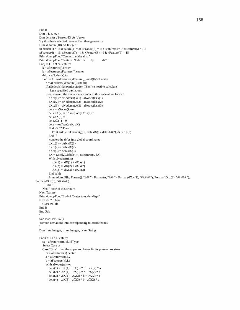
166
End If Dim i, j, k, m, n Dim delx As aTorsor, dX As Vector 'try this these selected features first then generalize Dim xFeature(10) As Integer xFeature(1) = 1: xFeature(2) = 2: xFeature(3) = 3: xFeature(4) = 9: xFeature(5) = 10: xFeature(6) = 11: xFeature(7) = 13: xFeature(8) = 14: xFeature(9) = 15 Print #dumpFile, "Center to nodes disp:" Print #dumpFile, "Feature Node dx dy dz" For j = 1 To 9 'nFeatures k = aFeatures(j).center k = aFeatures(xFeature(j)).center delx = aNodes(k).tor For i = 1 To aFeatures(xFeature(j)).nod(0) 'all nodes n = aFeatures(xFeature(j)).nod(i) If aNodes(n).knownDeviation Then 'no need to calculate ' keep specified deviations Else ' convert the deviation at center to this node along local-x dX.x(1) = aNodes(n).x(1) - aNodes(k).x(1) dX.x(2) = aNodes(n).x(2) - aNodes(k).x(2) dX.x(3) = aNodes(n).x(3) - aNodes(k).x(3) delx = aNodes(k).tor delx.dX(2) = 0 ' keep only dx, ry, rz delx.dX(3) = 0 delx.rX(1) = 0 delx = torTran(delx, dX) If xf <> "" Then Print #nFile, xFeature(j), n, delx.dX(1), delx.dX(2), delx.dX(3) End If 'convert the dx'es into global coordinates dX.x(1) = delx.dX(1) dX.x(2) = delx.dX(2) dX.x(3) = delx.dX(3) dX = Local2Global("F", xFeature(j), dX) With aNodes(n).tor .dX(1) = .dX(1) + dX.x(1) .dX(2) = .dX(2) + dX.x(2) .dX(3) = .dX(3) + dX.x(3) End With Print #dumpFile, Format(j, "### "); Format(n, "### "); Format(dX.x(1), "##.### "); Format(dX.x(2), "##.### ");
Format(dX.x(3), "##.###") End If Next ' node of this feature Next 'feature Print #dumpFile, "End of Center to nodes disp:" If xf <> "" Then Close #nFile End If End Sub ' Sub mapDev2Tol() 'convert deviations into corresponding tolerance zones ' Dim n As Integer, m As Integer, tx As String For n = 1 To nFeatures tx = aFeatures(n).tol.tolType Select Case tx Case "Size" 'find the upper and lower limits plus-minus sizes m = aFeatures(n).center a = aFeatures(n).Ly b = aFeatures(n).Lz With aNodes(m).tor delx(1) = .dX(1) + .rX(3) * b + .rX(2) * a delx(2) = .dX(1) + .rX(3) * b - .rX(2) * a delx(3) = .dX(1) - .rX(3) * b + .rX(2) * a delx(4) = .dX(1) - .rX(3) * b - .rX(2) * a

167
End With xmi = Abs(Min(delx(1), delx(2), delx(3), delx(4))) xma = Abs(Max(delx(1), delx(2), delx(3), delx(4))) aFeatures(n).tol.tolValue(1) = xma aFeatures(n).tol.tolValue(2) = xmi Case "Form" Case "Location" Case "Orientation" Case "Runout" Case "Profiel" Case Else End Select Next End Sub '---------------- Sub GenerateGeoConstraints() ' ' Modified from sub TorTransform to generates geometric continuity constraints for ' nodes commom to features of a part. Nilmani/June 20, 2002 ' Dim nRow As Integer, nCol As Integer, nFac As Integer, nP As Integer Dim kie As String, nR As Integer, nC As Integer, nodNow As Integer, nn As Integer Dim delx As Vector, nZero As Integer, nZero2 As Integer, xLink(3, 3) As Double Dim kTemp(6, 6) As Double, kTemp2(6, 6) As Double, nF As Integer, nF2 As Integer Dim xLCS(3, 3) As Double, nNod As Integer, nNod2 As Integer Dim nFeature As Integer, nFeature2 As Integer, actF(99) As Boolean ' ' use these temporary list to check the routine, generalize later actF(1) = True: actF(2) = True: actF(3) = True: actF(9) = True: actF(10) = True actF(11) = True: actF(13) = True: actF(14) = True: actF(15) = True ' delx.x(1) = 0: delx.x(2) = 0: delx.x(3) = 0 ' ' put these constraints after the asm constraints. nRow = LoopCount * 6 ' there are loopcount*6 equations ' 'Generate 3 equations for rows: nRow, nRow+1, nRow+2 ' For nP = 1 To nParts ' do for all parts For nF = 1 To aParts(nP).Features(0) ' for all Features of this part nFeature = aParts(nP).Features(nF) 'next Feature If actF(nFeature) Then 'remove later nZero = aFeatures(nFeature).center For nn = 1 To aFeatures(nFeature).nod(0) 'all nodes defining this feature nNod = aFeatures(nFeature).nod(nn) 'next node For nF2 = 1 To aParts(nP).Features(0) 'check other features If nF <> nF2 Then 'it's a different feature, check it nFeature2 = aParts(nP).Features(nF2) If actF(nFeature2) Then 'remove later nZero2 = aFeatures(nFeature2).center For nn2 = 1 To aFeatures(nFeature2).nod(0) 'all nodes of this feature nNod2 = aFeatures(nFeature2).nod(nn2) If nNod2 = nNod Then ' a nn is a node common to nF and nF2 'increment the row number 'nRow = nRow + 1 'MsgBox "nRow Part Feature Node Feature:" & nRow & ", " & nP & ", " & nF & ", " & nn & ", " & nF2 Debug.Print
"nRow Part Feature Node Feature:" & nRow & ", " & nP & ", " & nFeature & ", " & nNod & ", " & nFeature2 nCol = nn 'columns for these ' first transform t at nZero to nn For nR = 1 To 3 For nC = 1 To 3 xLCS(nR, nC) = aFeatures(nFeature).LCS(nR, nC) '3x3 local coordinate system Next Next nR delx.x(1) = aNodes(nNod).x(1) - aNodes(nZero).x(1) delx.x(2) = aNodes(nNod).x(2) - aNodes(nZero).x(2)

168
delx.x(3) = aNodes(nNod).x(3) - aNodes(nZero).x(3) 'Debug.Print "Cat, npf, row, col", Cat, npf, nRow, nCol ' transform and rotate the local values to global system ' and add to the corresponding cells in the global KMatrix ' First 3 rows - theta/rotational componenets ' For nR = 1 To 3 For nC = 1 To 3 kTemp(nR, nC) = xLCS(nR, nC) kTemp(nR, nC + 3) = 0 Next Next nR ' Last 3 rows - delta/linear components ' For nR = 1 To 3 kTemp(3 + nR, 1) = -delx.x(3) * xLCS(nR, 2) + delx.x(2) * xLCS(nR, 3) kTemp(3 + nR, 2) = -delx.x(1) * xLCS(nR, 3) + delx.x(3) * xLCS(nR, 1) kTemp(3 + nR, 3) = -delx.x(2) * xLCS(nR, 1) + delx.x(1) * xLCS(nR, 2) kTemp(3 + nR, 4) = kTemp(nR, 1) kTemp(3 + nR, 5) = kTemp(nR, 2) kTemp(3 + nR, 6) = kTemp(nR, 3) Next nR ' ' then transform t at nZero2 to nn2 ' For nR = 1 To 3 For nC = 1 To 3 xLCS(nR, nC) = aFeatures(nFeature2).LCS(nR, nC) '3x3 local coordinate system Next Next nR delx.x(1) = aNodes(nNod2).x(1) - aNodes(nZero2).x(1) delx.x(2) = aNodes(nNod2).x(2) - aNodes(nZero2).x(2) delx.x(3) = aNodes(nNod2).x(3) - aNodes(nZero2).x(3) ' For nR = 1 To 3 For nC = 1 To 3 kTemp2(nR, nC) = xLCS(nR, nC) kTemp2(nR, nC + 3) = 0 Next nC Next nR ' Last 3 rows - delta/linear components ' For nR = 1 To 3 kTemp2(3 + nR, 1) = -delx.x(3) * xLCS(nR, 2) + delx.x(2) * xLCS(nR, 3) kTemp2(3 + nR, 2) = -delx.x(1) * xLCS(nR, 3) + delx.x(3) * xLCS(nR, 1) kTemp2(3 + nR, 3) = -delx.x(2) * xLCS(nR, 1) + delx.x(1) * xLCS(nR, 2) kTemp2(3 + nR, 4) = kTemp2(nR, 1) kTemp2(3 + nR, 5) = kTemp2(nR, 2) kTemp2(3 + nR, 6) = kTemp2(nR, 3) Next nR ' finally post these terms in KTree ' ' 3 rows corresponding to nZero For nR = 1 To 3 For nC = 1 To 6 kie = "R" + Format(nRow + nR, "0000") + "C" + Format((nZero - 1) * 6 + nC, "0000") KTree.addNode nRow + nR, (nZero - 1) * 6 + nC, kie, kTemp(nR, nC) Next nC Next nR ' next same 3 rows corresponding to columns for nZero2 with negative values For nR = 1 To 3 For nC = 1 To 6 kie = "R" + Format(nRow + nR, "0000") + "C" + Format((nZero2 - 1) * 6 + nC, "0000") KTree.addNode nRow + nR, (nZero2 - 1) * 6 + nC, kie, -kTemp2(nR, nC) Next nC Next nR nRow = nRow + 3

169
' End If Next nn2 End If End If ' active features Next nF2 Next nn End If 'active features Next nF Next nP nC = 1 End Sub

170
Appendix - 9 Tolerance Synthesis Example –1: A 3-block system
1. Input data listing: (file: Art3M2-Oct22.art)
!A PLANAR 3-BLOCK ARTIFACT (3D) Model - 2 ! !Part #, Description, Center Node, Terminal?, LCS 9 values(11,12,13,....32,33) PART:, 1, MAIN BLOCK, 1, 1, 1,0,0,0,1,0,0,0,1 PART:, 2, LEFT BLOCK, 5, 0, 1,0,0,0,1,0,0,0,1 PART:, 3, RIGHT BLOCK, 12, 0, 1,0,0,0,1,0,0,0,1 ! ! FACE PART TYPE CENTER REF NODES/vertices FEATURE:, 1, 1, PLANE, 2, 20, 19,21,35,34 FEATURE:, 2, 1, PLANE, 8, 1, 32,33,35,34 FEATURE:, 3, 1, PLANE, 17, 27, 30,31,33,32 FEATURE:, 4, 1, PLANE, 29, 1, 30,31,28,27 FEATURE:, 5, 1, PLANE, 53, 1, 27,28,26,25 FEATURE:, 6, 1, PLANE, 24, 1, 25,26,23,22 FEATURE:, 7, 1, PLANE, 54, 1, 22,23,20,18 FEATURE:, 8, 1, PLANE, 55, 1, 18,20,21,19 FEATURE:, 9, 2, PLANE, 4, 5, 36,37,52,51 FEATURE:, 10, 2, PLANE, 6, 5, 41,42,52,51 FEATURE:, 11, 2, PLANE, 9, 5, 41,42,40,39 FEATURE:, 12, 2, PLANE, 38, 5, 39,40,37,36 FEATURE:, 13, 3, PLANE, 11, 12, 45,46,44,43 FEATURE:, 14, 3, PLANE, 13, 12, 45,46,48,47 FEATURE:, 15, 3, PLANE, 15, 12, 47,48,50,49 FEATURE:, 16, 3, PLANE, 56, 12, 43,44,50,49 ! !LINK: FROM FEATURE, TO FEATURE, GAP NODE, DOF, OTHER POINTS OF INTEREST LINK:,1, 9,3 LINK:,2,10,7 LINK:,2,14,14 LINK:,3,15,16 LINK:,11,13,10 ! !NODE X Y Z RX RY RZ DX DY DX (0=known/specified, ""=unknown) NODE:,1,0,10,0,0,0,0,0,0,0 NODE:,2,-60,45,0, 0,,,,0,0 NODE:,3,-60,45,0, 0,,,,0,0 NODE:,4,-60,45,0, 0,,,,0,0 NODE:,5,-30,45,0, ,,,,0,0 NODE:,6,-30,25,0, 0,,,,0,0 NODE:,7,-30,25,0, 0,,,,0,0 NODE:,8,0,25,0, 0,,,,0,0 NODE:,9,0,45,0, 0,,,,0,0 NODE:,10,0,45,0, 0,,,,0,0 NODE:,11,0,45,0, 0,,,,0,0 NODE:,12,20,45,0, ,,,,0,0 NODE:,13,20,25,0, 0,,,,0,0 NODE:,14,20,25,0, 0,,,,0,0 NODE:,15,40,45,0, 0,,,,0,0 NODE:,16,40,45,0, 0,,,,0,0 NODE:,17,40,45,0, 0,,,,0,0 NODE:,18,-90,80,20,0,0,0,0,0,0,0 NODE:,19,-60,80,20,0,0,0,0,0,0,0 NODE:,20,-90,80,-20,0,0,0,0,0,0,0

171
NODE:,21,-60,80,-20,0,0,0,0,0,0,0 NODE:,22,-90,0,20,0,0,0,0,0,0,0 NODE:,23,-90,0,-20,0,0,0,0,0,0,0 NODE:,24,0,0,0,0,0,0,0,0,0,0 NODE:,25,70,0,20,0,0,0,0,0,0,0 NODE:,26,70,0,-20,0,0,0,0,0,0,0 NODE:,27,70,80,20,0,0,0,0,0,0,0 NODE:,28,70,80,-20,0,0,0,0,0,0,0 NODE:,29,55,80,0,0,0,0,0,0,0,0 NODE:,30,40,80,20,0,0,0,0,0,0,0 NODE:,31,40,80,-20,0,0,0,0,0,0,0 NODE:,32,40,25,20,0,0,0,0,0,0,0 NODE:,33,40,25,-20,0,0,0,0,0,0,0 NODE:,34,-60,25,20,0,0,0,0,0,0,0 NODE:,35,-60,25,-20,0,0,0,0,0,0,0 NODE:,36,-60,65,20,0,0,0,0,0,0,0 NODE:,37,-60,65,-20,0,0,0,0,0,0,0 NODE:,38,-30,65,0,0,0,0,0,0,0,0 NODE:,39,0,65,20,0,0,0,0,0,0,0 NODE:,40,0,65,-20,0,0,0,0,0,0,0 NODE:,41,0,25,20,0,0,0,0,0,0,0 NODE:,42,0,25,-20,0,0,0,0,0,0,0 NODE:,43,0,65,20,0,0,0,0,0,0,0 NODE:,44,0,65,-20,0,0,0,0,0,0,0 NODE:,45,0,25,20,0,0,0,0,0,0,0 NODE:,46,0,25,-20,0,0,0,0,0,0,0 NODE:,47,40,25,20,0,0,0,0,0,0,0 NODE:,48,40,25,-20,0,0,0,0,0,0,0 NODE:,49,40,65,20,0,0,0,0,0,0,0 NODE:,50,40,65,-20,0,0,0,0,0,0,0 NODE:,51,-60,25,20,0,0,0,0,0,0,0 NODE:,52,-60,25,-20,0,0,0,0,0,0,0 NODE:,53,70,40,0,0,0,0,0,0,0,0 NODE:,54,-90,40,0,0,0,0,0,0,0,0 NODE:,55,-75,80,0,0,0,0,0,0,0,0 NODE:,56,20,65,0,0,0,0,0,0,0,0 ! ! following DISP data is used for computations involving the deviations from Matlab optimuzation run. DISP:, 2, 0.0000, 0.0100, 0.0100, 0.0100, -0.0000, 0.0000 DISP:, 3, 0.0000, -0.0054, -0.0100, 0.0100, 0.0000, 0.0000 DISP:, 4, -0.0000, -0.0047, 0.0000, 0.0063, -0.0000, 0.0000 DISP:, 6, -0.0000, 0.0008, -0.0000, 0.0010, 0.0000, 0.0000 DISP:, 7, 0.0000, 0.0001, 0.0000, -0.0023, -0.0000, 0.0000 DISP:, 8, -0.0000, 0.0100, -0.0000, 0.0100, 0.0000, 0.0000 DISP:, 9, 0.0000, 0.0100, 0.0050, -0.0100, -0.0000, -0.0000 DISP:, 10, 0.0000, -0.0002, -0.0100, -0.0100, -0.0000, 0.0000 DISP:, 11, 0.0000, 0.0100, 0.0050, -0.0100, 0.0000, 0.0000 DISP:, 13, 0.0000, 0.0008, -0.0000, 0.0100, 0.0000, 0.0000 DISP:, 14, 0.0000, -0.0003, -0.0000, -0.0067, 0.0000, 0.0000 DISP:, 15, 0.0000, -0.0051, 0.0000, 0.0017, 0.0000, 0.0000 DISP:, 16, 0.0000, 0.0055, 0.0100, -0.0100, 0.0000, 0.0000 DISP:, 17, 0.0000, 0.0100, 0.0100, 0.0100, 0.0000, 0.0000 2. Generated Cost Functions
function yy = costfunJun25R1 (x) % deviation dependent cost of manufacturing formulation % generated from tnp3. Nilmani Pramanik / Jun 25, 2002 global CC; yy = 0; yy = yy + 2200 /( .00001 + abs(x(10)+ 55*x(8)+ 40*x(9) ));

172
yy = yy + 4000 /( .00001 + abs(x(46)+ 100*x(44)+ 40*x(45) )); yy = yy + 2200 /( .00001 + abs(x(100)+ 55*x(98)+ 40*x(99) )); yy = yy + 1600 /( .00001 + abs(x(22)+ 40*x(20)+ 40*x(21) )); yy = yy + 2400 /( .00001 + abs(x(34)+ 60*x(32)+ 40*x(33) )); yy = yy + 1600 /( .00001 + abs(x(52)+ 40*x(50)+ 40*x(51) )); yy = yy + 1600 /( .00001 + abs(x(64)+ 40*x(62)+ 40*x(63) )); yy = yy + 1600 /( .00001 + abs(x(76)+ 40*x(74)+ 40*x(75) )); yy = yy + 1600 /( .00001 + abs(x(88)+ 40*x(86)+ 40*x(87) )); CC=CC+1; if mod(CC,100) == 0 CC yy end
3. Assemblability Equations Each equation shown below as Eqn# is generated from the assemblability constraint Kx=b for the example problem. Each term on the left hand side of an equation is of the form: <r|d><X|Y|Z><N>, where r stands for rotation and d for displacement. X, Y, and Z are the local axes, and N is the node number. For example rX(4) indicates rotational component of the deviation at node 4 in local X direction.
Eqn# 1: rX(2)+ rX(3)+ rX(4)- rX(5)- rZ(6)+ rZ(7)- rZ(8) = 0
Eqn# 2: rZ(2)- rZ(3)- rZ(4)- rY(5)- rX(6)+ rX(7)- rX(8) = 0
Eqn# 3: rY(2)+ rY(3)- rY(4)- rZ(5)+ rY(6)+ rY(7)- rY(8) = 0
Eqn# 4: -35. *rZ(2)+ dX(2)- 35. *rZ(3)+ dX(3)- 35. *rZ(4)+ dX(4)+35. *rZ(5)- dX(5)- 15. *rX(6)- 30. *rY(6)- dZ(6)+15. *rX(7)+30. *rY(7)+ dZ(7)- 15. *rX(8)- dZ(8) = 0
Eqn# 5: -35. *rX(2)- 60. *rY(2)- dZ(2)- 35. *rX(3)- 60. *rY(3)- dZ(3)- 35. *rX(4)- 60. *rY(4)- dZ(4)+30. *rZ(5)- dY(5)+15. *rZ(6)- dX(6)- 15. *rZ(7)+ dX(7)+15. *rZ(8)- dX(8) = 0
Eqn# 6: -60. *rZ(2)+ dY(2)- 60. *rZ(3)+ dY(3)+60. *rZ(4)- dY(4)- 35. *rX(5)- 30. *rY(5)- dZ(5)- 30. *rZ(6)+ dY(6)- 30. *rZ(7)+ dY(7)- dY(8) = 0
Eqn# 7: rX(2)+ rX(3)+ rX(4)- rX(5)- rZ(8)+ rX(9)+ rX(10)+ rX(11)- rX(12)- rZ(13)+ rZ(14) = 0
Eqn# 8: rZ(2)- rZ(3)- rZ(4)- rY(5)- rX(8)- rZ(9)- rZ(10)- rZ(11)- rY(12)- rX(13)+ rX(14) = 0
Eqn# 9: rY(2)+ rY(3)- rY(4)- rZ(5)- rY(8)+ rY(9)+ rY(10)- rY(11)- rZ(12)+ rY(13)+ rY(14) = 0
Eqn# 10: -35. *rZ(2)+ dX(2)- 35. *rZ(3)+ dX(3)- 35. *rZ(4)+ dX(4)+35. *rZ(5)- dX(5)- 15. *rX(8)- dZ(8)- 35. *rZ(9)+ dX(9)- 35. *rZ(10)+ dX(10)- 35. *rZ(11)+ dX(11)+35. *rZ(12)- dX(12)- 15. *rX(13)+20. *rY(13)- dZ(13)+15. *rX(14)- 20. *rY(14)+ dZ(14) = 0
Eqn# 11: -35. *rX(2)- 60. *rY(2)- dZ(2)- 35. *rX(3)- 60. *rY(3)- dZ(3)- 35. *rX(4)- 60. *rY(4)- dZ(4)+30. *rZ(5)- dY(5)+15. *rZ(8)- dX(8)- 35. *rX(9)- dZ(9)- 35. *rX(10)- dZ(10)- 35. *rX(11)- dZ(11)- 20. *rZ(12)- dY(12)+15. *rZ(13)- dX(13)- 15. *rZ(14)+ dX(14) = 0
Eqn# 12: -60. *rZ(2)+ dY(2)- 60. *rZ(3)+ dY(3)+60. *rZ(4)- dY(4)- 35. *rX(5)- 30. *rY(5)- dZ(5)- dY(8)+ dY(9)+ dY(10)- dY(11)- 35. *rX(12)+20. *rY(12)- dZ(12)+20. *rZ(13)+ dY(13)+20. *rZ(14)+ dY(14) = 0
Eqn# 13: rX(2)+ rX(3)+ rX(4)- rX(5)+ rX(9)+ rX(10)+ rX(11)- rX(12)+ rX(15)- rX(16)+ rX(17) = 0
Eqn# 14: rZ(2)- rZ(3)- rZ(4)- rY(5)- rZ(9)- rZ(10)- rZ(11)- rY(12)- rZ(15)+ rZ(16)- rZ(17) = 0
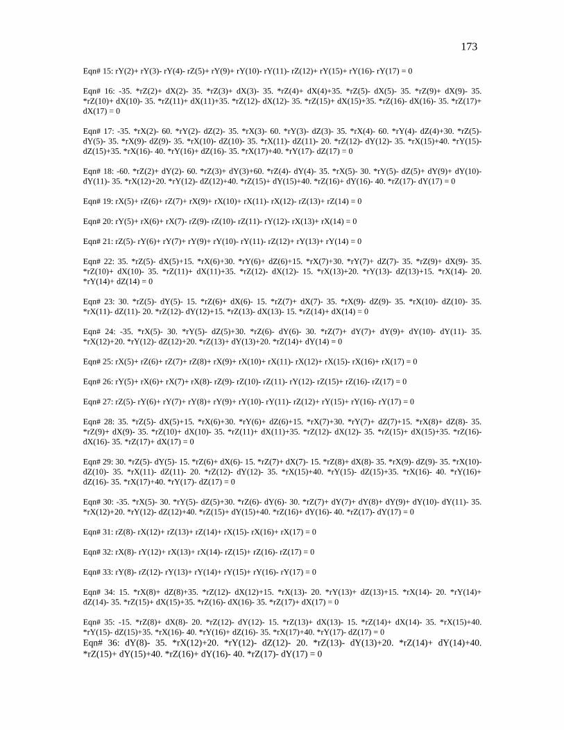
173
Eqn# 15: rY(2)+ rY(3)- rY(4)- rZ(5)+ rY(9)+ rY(10)- rY(11)- rZ(12)+ rY(15)+ rY(16)- rY(17) = 0
Eqn# 16: -35. *rZ(2)+ dX(2)- 35. *rZ(3)+ dX(3)- 35. *rZ(4)+ dX(4)+35. *rZ(5)- dX(5)- 35. *rZ(9)+ dX(9)- 35. *rZ(10)+ dX(10)- 35. *rZ(11)+ dX(11)+35. *rZ(12)- dX(12)- 35. *rZ(15)+ dX(15)+35. *rZ(16)- dX(16)- 35. *rZ(17)+ dX(17) = 0
Eqn# 17: -35. *rX(2)- 60. *rY(2)- dZ(2)- 35. *rX(3)- 60. *rY(3)- dZ(3)- 35. *rX(4)- 60. *rY(4)- dZ(4)+30. *rZ(5)- dY(5)- 35. *rX(9)- dZ(9)- 35. *rX(10)- dZ(10)- 35. *rX(11)- dZ(11)- 20. *rZ(12)- dY(12)- 35. *rX(15)+40. *rY(15)- dZ(15)+35. *rX(16)- 40. *rY(16)+ dZ(16)- 35. *rX(17)+40. *rY(17)- dZ(17) = 0
Eqn# 18: -60. *rZ(2)+ dY(2)- 60. *rZ(3)+ dY(3)+60. *rZ(4)- dY(4)- 35. *rX(5)- 30. *rY(5)- dZ(5)+ dY(9)+ dY(10)- dY(11)- 35. *rX(12)+20. *rY(12)- dZ(12)+40. *rZ(15)+ dY(15)+40. *rZ(16)+ dY(16)- 40. *rZ(17)- dY(17) = 0
Eqn# 19: rX(5)+ rZ(6)+ rZ(7)+ rX(9)+ rX(10)+ rX(11)- rX(12)- rZ(13)+ rZ(14) = 0
Eqn# 20: rY(5)+ rX(6)+ rX(7)- rZ(9)- rZ(10)- rZ(11)- rY(12)- rX(13)+ rX(14) = 0
Eqn# 21: rZ(5)- rY(6)+ rY(7)+ rY(9)+ rY(10)- rY(11)- rZ(12)+ rY(13)+ rY(14) = 0
Eqn# 22: 35. *rZ(5)- dX(5)+15. *rX(6)+30. *rY(6)+ dZ(6)+15. *rX(7)+30. *rY(7)+ dZ(7)- 35. *rZ(9)+ dX(9)- 35. *rZ(10)+ dX(10)- 35. *rZ(11)+ dX(11)+35. *rZ(12)- dX(12)- 15. *rX(13)+20. *rY(13)- dZ(13)+15. *rX(14)- 20. *rY(14)+ dZ(14) = 0
Eqn# 23: 30. *rZ(5)- dY(5)- 15. *rZ(6)+ dX(6)- 15. *rZ(7)+ dX(7)- 35. *rX(9)- dZ(9)- 35. *rX(10)- dZ(10)- 35. *rX(11)- dZ(11)- 20. *rZ(12)- dY(12)+15. *rZ(13)- dX(13)- 15. *rZ(14)+ dX(14) = 0
Eqn# 24: -35. *rX(5)- 30. *rY(5)- dZ(5)+30. *rZ(6)- dY(6)- 30. *rZ(7)+ dY(7)+ dY(9)+ dY(10)- dY(11)- 35. *rX(12)+20. *rY(12)- dZ(12)+20. *rZ(13)+ dY(13)+20. *rZ(14)+ dY(14) = 0
Eqn# 25: rX(5)+ rZ(6)+ rZ(7)+ rZ(8)+ rX(9)+ rX(10)+ rX(11)- rX(12)+ rX(15)- rX(16)+ rX(17) = 0
Eqn# 26: rY(5)+ rX(6)+ rX(7)+ rX(8)- rZ(9)- rZ(10)- rZ(11)- rY(12)- rZ(15)+ rZ(16)- rZ(17) = 0
Eqn# 27: rZ(5)- rY(6)+ rY(7)+ rY(8)+ rY(9)+ rY(10)- rY(11)- rZ(12)+ rY(15)+ rY(16)- rY(17) = 0
Eqn# 28: 35. *rZ(5)- dX(5)+15. *rX(6)+30. *rY(6)+ dZ(6)+15. *rX(7)+30. *rY(7)+ dZ(7)+15. *rX(8)+ dZ(8)- 35. *rZ(9)+ dX(9)- 35. *rZ(10)+ dX(10)- 35. *rZ(11)+ dX(11)+35. *rZ(12)- dX(12)- 35. *rZ(15)+ dX(15)+35. *rZ(16)- dX(16)- 35. *rZ(17)+ dX(17) = 0
Eqn# 29: 30. *rZ(5)- dY(5)- 15. *rZ(6)+ dX(6)- 15. *rZ(7)+ dX(7)- 15. *rZ(8)+ dX(8)- 35. *rX(9)- dZ(9)- 35. *rX(10)- dZ(10)- 35. *rX(11)- dZ(11)- 20. *rZ(12)- dY(12)- 35. *rX(15)+40. *rY(15)- dZ(15)+35. *rX(16)- 40. *rY(16)+ dZ(16)- 35. *rX(17)+40. *rY(17)- dZ(17) = 0
Eqn# 30: -35. *rX(5)- 30. *rY(5)- dZ(5)+30. *rZ(6)- dY(6)- 30. *rZ(7)+ dY(7)+ dY(8)+ dY(9)+ dY(10)- dY(11)- 35. *rX(12)+20. *rY(12)- dZ(12)+40. *rZ(15)+ dY(15)+40. *rZ(16)+ dY(16)- 40. *rZ(17)- dY(17) = 0
Eqn# 31: rZ(8)- rX(12)+ rZ(13)+ rZ(14)+ rX(15)- rX(16)+ rX(17) = 0
Eqn# 32: rX(8)- rY(12)+ rX(13)+ rX(14)- rZ(15)+ rZ(16)- rZ(17) = 0
Eqn# 33: rY(8)- rZ(12)- rY(13)+ rY(14)+ rY(15)+ rY(16)- rY(17) = 0
Eqn# 34: 15. *rX(8)+ dZ(8)+35. *rZ(12)- dX(12)+15. *rX(13)- 20. *rY(13)+ dZ(13)+15. *rX(14)- 20. *rY(14)+ dZ(14)- 35. *rZ(15)+ dX(15)+35. *rZ(16)- dX(16)- 35. *rZ(17)+ dX(17) = 0
Eqn# 35: -15. *rZ(8)+ dX(8)- 20. *rZ(12)- dY(12)- 15. *rZ(13)+ dX(13)- 15. *rZ(14)+ dX(14)- 35. *rX(15)+40. *rY(15)- dZ(15)+35. *rX(16)- 40. *rY(16)+ dZ(16)- 35. *rX(17)+40. *rY(17)- dZ(17) = 0 Eqn# 36: dY(8)- 35. *rX(12)+20. *rY(12)- dZ(12)- 20. *rZ(13)- dY(13)+20. *rZ(14)+ dY(14)+40. *rZ(15)+ dY(15)+40. *rZ(16)+ dY(16)- 40. *rZ(17)- dY(17) = 0

174
Bibliography
ASME (1994) ASME Dimensioning and Tolerancing. ASME Standard Y14.5M, American Society of Mechanical Engineering, New York, 1994.
Ballot, E., Bourdet, P., (1998) A Computation Method for the Consequences of
Geometric Errors in Mechanisms. Geometric Design Tolerancing: Theories, Standards and Applications, Hoda A. Elmaraghy (Editor), Chapman & Hall, pp 197-207, 1998.
Ballot, E., Bourdet, P., (2000) A Mathematical Model of Geometric Errors in the case of
Specification and 3D Control of Mechanical Parts. Advanced Mathematical and Computational Tools in Metrology IV, 2000 World Scientific Publishing
Baxter, J. E., Juster, N. P. and Pennington, A. de. (1994) Verification of Product
Design Specifications Using a Functional Data Model. MOSES Project Research Report 25, University of Leeds, April 1994.
Bharadwaj, B. (1995) A Framework for Tolerance Synthesis of Mechanical
Components. Master's Thesis. Syracuse University, Syracuse, NY, 1995. Billo, R. E. (1989) An Object-Oriented Modeling Methodology Utilizing Conceptual
Graphs for Form Feature Definition, Ph.D. Thesis, Arizona State University, 1989.
Bracewell, R. H., Chaplin, R. V. , Langdon, P. M. , Li, M., Oh, V. K. , Sharpe, J. E. E.
and Yan, X. T. (1995) Integrated Platform for AI Support of Complex Design. In AI System Support for Conceptual Design (Editor: J. E. E. Sharpe), Springer-Verlag, 1995.
Broman, V. and Shensa, M. J. (1990) A Compact Algorithm for the Intersection and
Approximation of N-Dimensional Polytopes. Mathematics and Computers in Simulation, vol. 32, pp. 469-480, 1990.
Chandrasekaran, B. , Goel, A. K. and Iwasaki, Y. (1993) Functional Representation of
Design Rationale. Computer, pp. 48-6, January 1993. Chandrasekaran, B. and Josephson, J. R. (1996) An explication of Function. Laboratory
for AI Research, The Ohio State University, Columbus, OH, January 1996. Chase, K. W., Greenwood, W.H.,Loosli, B.G. and Hauglund, L.F. (1990) Least cost
tolerance allocation for mechanical assemblies with automated process selection. Manufacturing Review, vol. 3(1) pp. 49-59, 1990.

175
Chase, K. W. and Magleby, Spencer P. (1997) A Comprehensive System for Computer-Aided Tolerance Analysis of 2-D and 3-D Mechanical Assemblies. Proceedings of the 5th International Seminar on Computer-Aided Tolerancing Toronto, Canada, April 27-29, 1997.
Chen, Mu-Chen. (2001) Tolerance synthesis by neural learning and nonlinear
programming, International Journal of Production Economics, vol. 70, no.1, pp. 55-65, Mar 2001.
Ciarallo, Frank W., Yang, C.C. (1997) Optimization of propagation in interval constraint
networks for tolerance design. Proceedings of the IEEE International Conference on Systems, Man and Cybernetics, vol. 2, pp. 1924-1929, 1997.
Cutkosky, M. R., Engelmore, R. S., et al. (1993) PACT: An Experiment in Integrating
Concurrent Engineering Systems. IEEE Computer, pp. 28-37, 1993. Dasgupta, D. , Michalewicz, Z. (1997) Evolutionary Algorithms in Engineering
Applications, Springer-Verlag, 1997. Deng, J. ,Deng, S. (2002) The adaptive branch and bound method of tolerance synthesis
based on the reliability index, International Journal of Advanced Manufacturing Technology, vol. 20, no. 3, pp. 190-200, 2002.
Ding, Y. , Jin, J., Ceglarek, D. andShi, J. (2000) Process-Oriented Tolerance Synthesis
for Multistage Manufacturing Processes, presented on the ASME International Mechanical Engineering Congress and Exposition’2000.
Dong, Z. Hu, W. and Xue, D. (1994) New Production Cost-Tolerance Models for
Tolerance Synthesis, Journal of Engineering for Industry, Transaction of ASME, Vol. 116, pp. 199-206, 1994.
Dong, Z. (1997) Chapter 9: Tolerance Synthesis by Manufacturing Cost Modeling and
Design Optimization. Advanced Tolerancing Techniques, H. C. Zhang (Ed.), John Wiley & Sons, pp. 233-260, 1997.
Dong, Z., Wang, G. (1998) Automated Cost Modeling for Tolerance Synthesis Using
Manufacturing Process Data, Knowledge Reasoning and Optimization. Geometric Design Tolerancing, Kluwer Academic, H. A. ElMaraghy (Ed.), pp. 282-293, 1998.
Drake, Paul (1999) Dimensioning and Tolerancing Handbook, McGraw-Hill, 1999 Du, R., Ji, Shuping; Li, Xiaoli (2000) Tolerance synthesis using second-order fuzzy
comprehensive evaluation and genetic algorithm. International Journal of Production Research, vol. 38, no. 15, pp. 3471-3483, 2000.

176
Due, Mark J. , Constantin, Chassapis (1996) Tolerance design synthesis in a concurrent engineering environment. Proceedings of the 1996 ASME International Mechanical Engineering Congress and Exposition, Nov 17-22 1996, Atlanta, GA, USA.
Feng, C-X., Kusiak, A. (2000) Robust Tolerance Design with the Design of Experiments
Approach. Transactions of the ASME, Journal of Manufacturing Science and Engineering, vol. 122(3), pp. 520-528, 2000.
Finger, S. and Rinderle, J. R. (1989) A Transformational Approach to Mechanical
Design Using Bond Graph Grammer. In Proc. of 1st ASME Design Theory and Methodology Conference, pp. 197-216, 1989.
Finger, S., Fox, M. S., Navinchandra, D. , Prinz, F. B. and Rinderle, J. R. (1990)
Design Fusion: A Product Life-cycle View for Engineering Designs. Technical Report EDRC 24-28-90, EDRC, CMU, 1990.
Finger, S., Fox, M. S., Prinz, F. B. and Rinderle, J. R. (1992) Concurrent Design.
Applied Artificial Intelligence, vol. 6, pp. 257-283, 1992. Gilbert, Olivier L., (1992) Representation of Geometric Variations Using Matrix
Transforms for Statistical Tolerance Analysis in Assemblies. Master thesis, MIT, 1992.
Gorti, S. R. and Sriram, Ram D. (1996) From Symbol to Form: A Framework for
Conceptual Design. Computer-Aided Design, vol. 28, no. 11, pp. 853-870, 1996. Greenwood, W. H., Chase, K.W. (1987) A new tolerance analysis method for designers
and manufacturers. Journal of Engineering for Industry, 109:112-116, 1987 Gui, J. K. and Mantyla, M. (1994) Functional Understanding of Assembly Modelling.
Computer_Aided Design, vol. 26, no. 6, pp. 435-451, 1994. Henson, B., Juster, N. P. and Pennington, A. de. (1994) Towards an Integrated
Representation of Function, Behavior and Form. MOSES Project Research Report 16, University of Leeds, April 1994.
Hoover, S. P. and Rinderle, J. R. 1989) A Synthesis Strategy for Mechanical Devices.
Research in Engineering Design, Vol. 1, No. 2, pp 87-103, 1989. Hundal, M. S. and Byrne, J. F. (1991) Computer-Aided Generation of Function Block
Diagrams in a Methodical Design Procedure. In Proc. of Design Theory and Methodology- DTM'91 Conference, Volume DE-Vol.27, pp. 251-257, 1991.
177
Iannuzzi, Mark (1998) Variation simulation for tolerance analysis and synthesis. Proceedings of the 1998 ASQ's 52nd Annual Quality Congress, May 4-6 1998, Philadelphia, PA, USA.
Iwasaki, Y. and Simon, H. A. (1986) Causality in Device Behavior. Artificial
Intelligence, vol. 29(1), pp. 3-32, 1986. Iyengar, G., Lee, C-L and Kota, S. (1994) Towards an Objective Evaluation of Alternate
Designs. ASME Journal of Mechanical Design, vol. 116, pp. 487-492, 1994. Jayaraman, R., Srinivasan, V. (1989) Geometric Tolerancing Part I: Virtual Boundary
requirements. IBM Journal of Research and Development, vol. 33(2), 1989. Jayaraman, R., Srinivasan, V. (1989) Geometric Tolerancing Part II: Cinditional
Tolerances. IBM Journal of Research and Development, vol. 33(2), 1989. Johnson, A. L. (1990) Functional Modeling: A New Development in Computer-Aided
Design. Intelligent CAD (Editors: H. Yoshikawa and T. Holden), Vol. II, pp. 203-212. Elsevier Science Publishers B. V., North Holland, Amsterdam, 1990.
Kannapan, S. M. and Marshek, K. M. (1991) Design Synthesis Reasoning: A
Methodology for Mechanical Design. Research in Engineering Design, vol. 2, No. 4, pp 221-238, 1991.
Kapur, K. C., Raman, S. and Pulat, P.S. (1990) Methodology for tolerance design using
quality loss function. Computers and Industrial Engineering, vol. 19, pp. 254-257, 1990.
Kota, S. (1990) A Qualitative Matrix Representation Scheme for the Conceptual Design
of Mechanisms. In Proc. of ASME Design Automation Conference (21st Biannual ASME Mechanisms Conference), pp. 217-230, 1990.
Krause, F. L.., Kimura, F., Kjellberg, T. and Lu, S. C-Yu. (1993) Product Modelling.
Annals of CIRP, vol. 42, no. 2, pp. 695-706, 1993. Krishnaswami, M. and Mayne, R.W. (1994) Optimizing tolerance allocation for
minimum cost and maximum quality. Proc. ASME Design Automation Conference, 20th Design Automation Conference, number DE-vol.69-1, pp. 211-217, 1994.
Lai, K. and Wilson, W. R. D. (1989) FDL - A Language for Function Description and
Realization in Mechanical Design. Journal of Mechanisms, Transmissions, and Automation in Design. Transactions of the ASME, vol. 111, pp. 117-123, 1989.

178
Laperriere, L., ElMaraghy, Hoda A. (2000) Tolerance analysis and synthesis using Jacobian transforms, CIRP Annals - Manufacturing Technology, vol. 49, no. 1, pp. 359-362, 2000.
Lee, Woo-Jong, Woo, Tony C.; Chou, Shuo-Yan, (1993) Tolerance synthesis for
nonlinear systems based on nonlinear programming, IIE Transactions, vol. 25, no. 1, pp. 51-61, 1993.
Lin, Shui-Shun, Wang, Hsu-Pin (Ben) and Zhang, Chun (Chuc) (1997) Optimal
Tolerance Design for Integrated Design, Manufacturing, and Inspection with Genetic Algorithms. Advanced Tolerancing Techniques, Hong-Chao Zhang (Editor), John Wiley & Sons, Inc, pp 261-281, 1997.
Mantripragada, R. and Whitney, D. E. (1998) The Datum Flow Chain: A Systematic
Approach to Assembly Design and Modeling. Research in Engineering Design, vol 10, pp. 150-165, 1998.
Mathieu, L., Clement, A. and Bourdet, P. (1998) Modeling, Representation and
Processing of Tolerances, Tolerance Inspection: A Survey of Current Hypothesis. Geometric Design Tolerancing: Theories, Standards and Applications, Hoda A. Elmaraghy (Editor), Chapman & Hall, pp 1-33, 1998.
Moore, R.E. (1966) Interval Analysis, Prentice-Hall, Englewood Cliffs, N.J. Moskowitz, H., Plante, R. , Duffy, J. (2001) Multivariate tolerance design using quality
loss, Source: IIE Transactions, vol. 33, no. 6, pp. 437-448, 2001. Nagarwala, M.Y. , Pulat, P.S. and Raman, S.R. (1994) Process selection and tolerance
allocation for minimum cost assembly. Manufacturing Science and Engineering, 116, 1994.
Nurre, J. H., Vedati, K. (1998) Cost optimization of a process plan's tolerance
assignments for manufacturing, nternational Journal of Modelling & Simulation, vol. 18, no. 3, pp. 196-200, 1998.
Pahl, G. and Beitz, W. (1984) Engineering Design. Springer-Verlag, 1984. Pramanik, N., Roy, U., Wang, H., Sudarsan, R., Sriram, R. D., Lyons, K. W. (2003a)
Tolerance Synthesis Scheme. NIST IR 6836, (2003), National Institute of Standards and Technology, Gaithersburg, Maryland.
Pramanik, N., Roy, U., Sudarsan, R., Sriram, R. D., Lyons, K. W. (2003b) Syntheis of
Geometric Tolerances of a Gearbox using a Deviation-based Tolerance Synthesis Scheme, DETC2003/CIE-48192 Proceedings of ASME 2003 Design Engineering Technical Conferences, Chicago, Illinois USA, September 2-6, 2003
179
Pramanik, N., Roy, U., Sudarsan, R., Sriram, R. D., Lyons, K. W. (2003c) A Generic Deviation-based Approach for Synthesis of Tolerances. Accepted for publication in IEEE Transactions on Robotics and Automation
Quipers, Benjamin (1994) Qualitative Reasoning. Modeling and Simulation with
Incomplete Knowledge, The MIT Press, 1994. Rajagopalan,S. and Cutkoswky, M. R. (1998) “Tolerance Representation for
Mechanism Assemblies in Layered manufacturing”, DETC98/DFM-5726, Proc. of ASME Design Engineering Technical Conferences, Atlanta, Ga, 1998.
Rajan, Venkat N. , Lyons, K. W. and Sreerngam, Raj (1997) Assembly Representations
for Capturing Mating Constraints and Component Kinematics. Proceedings of the 1997 IEEE Int. Sym. on Assembly and Task Planning, Marina del Rey, CA, pp. 206-211, 1997.
Reddy, S. Y. (1994) Hierarchical and Interactive Parameter Refinement for Early-Stage
System Design. PhD Thesis, University of Illinois at Urbana-Champaign, 1994. Requicha, A. A. (1983) Towards a theory of gemetric tolerancing, International Journal
of Robotics Research, vol. 2(4), pp. 45-60, 1983. Roy, U. and Liu,C.R. (1988a) Feature-Based Representational Scheme of a Solid
Modeler for Providing Dimensioning and Tolerancing Information, Robotics & Computer-Integrated Manufacturing, vol. 4, no. 3-4, pp. 335-345, 1988.
Roy, U. and Liu,C.R.. (1988b) Establishment of Functional Relationships between the
Product Components in Assembly Data Base. J. Computer-Aided Design, vol. 20, no. 10, pp. 570-580, 1988.
Roy, U. , Pollard, M.C., Mantooth, K. and Liu, C.R. (1989) Tolerance Representation
Scheme in Solid Modeling: Part I & II, ASME Advances in Design Automation Conference, , pp. 1-17, Montreal, 1989.
Roy, U., Banerjee, P. and Liu, C. R. (1990) Design of an Automated Assembly
Environment. Computer-Aided Design, vol. 21 no. 9, pp. 561-569, 1989. (also published in Robotics, Automation and Management in Manufacturing Bulletin, vol. 7, issue 1, 1990).
Roy, U., Liu, C.R. and Woo, T.C. (1991) Review of Dimensioning and Tolerancing:
Representation and Processing, Computer-Aided Design, vol. 23, no. 7, pp. 466-483, 1991.
Roy, U., Bharadwaj, B., Chavan, A. and Mohan, C. K. (1995) Development of a
Feature Based Expert Manufacturing Process Planner. Proc. of the 7th IEEE International Conference on Tools with Artificial Intelligence, pp. 65-73, 1995.

180
Roy, U. and Bharadwaj, B. (1996) Tolerance Synthesis in a Product Design System.
Technical Paper# MS96-146. North American Manufacturing Research Institution. Society of Manufacturing Engineers, Dearborn, MI, 1996.
Roy,U. and Fang, Ying-Che (1997) Optimal Tolerance Re-allocation for the Generative
Process Sequence. IIE Transactions, vol 29, pp 37-44, 1997. Roy, U., Li, Bing (1997) Tolerance Synthesis by Manufacturing Cost Modeling and
Design Optimization, Advanced Tolerancing Techniques, Edited by Hong-Chao Zhang, John Wiley & Sons, Inc, pp 233-260, 1997.
Roy, U., Li, Bing. (1998) Representation and Interpretation of Geometric Tolerances for
Polyhedral Objects - I. Form Tolerances. J. Computer-Aided Design, vol. 30, no.2, pp. 151-161, 1998.
Roy, U., Sudarsan, R., Sriram, R. D. , Lyons, K. W. and Duffey, M. R. (1999a)
Information Architecture for Design Tolerancing: from Conceptual to the Detail Design, accepted for presentation and publication in the Proc. of DETC'99, 1999 ASME International Design Engineering Technical Conferences, September 12-15, 1999, Nevada, Las Vegas, USA.
Roy, U. and Li, B. (1999b) Representation and Interpretation of Geometric Tolerances
for Polyhedral Objects - II. Size, Orientation and Positional Tolerances. J. of Computer Aided Design, vol. 31, no. 4, pp. 273-285, 1999.
Roy, U. and Li. B. (1999c) Representation and interpretation of geometric tolerances for
polyhedral objects-II. Size, orientation and position tolerances. Computer-Aided Design, vol. 31, pp 273-285, 1999.
Roy, U., Sudarsan, R., Narahari, Y., Sriram, R. D., Lyons, K. W., Duffey, M. R. and
Pramanik, N. (2000) Information Models for Design Tolerancing: From Conceptual to the Detail Design. Technical Report, National Institute of Standards and Technology, NIST IR 6524, 2000.
Roy, U., Pramanik, N., Sudarsan, R. , Sriram, R. D. and Lyons, K. W., (2001)
Function-to-Form Mapping: Model, Representation and Applications in Design Synthesis. Computer-Aided Design vol. 33, no. 10, pp 699-720, 2001.
Schmekel, H . (1989) Functional Models and Design Solutions. Annals of CIRP, vol. 38,
pp. 129-132, 1989. Shan, A. , Roth, R. N., Wilson, R. J. (1999) A new approach to statistical geometrical
tolerance analysis. International Journal of Advanced Manufacturing Technology, vol. 15, no. 3, p 222-30, 1999.

181
Shaw, N. K., Bloor, M. S. and Pennington, A. de (1989) Product Data Models. Research in Engineering Design, vol. 1, pp. 43-50, 1989.
Skowronski, V. J., Turner, J. U. (1997) Using Monte-Carlo variance reduction in
statistical tolerance synthesis. Computer Aided Design, vol. 29, no. 1, pp. 63-69, 1997.
Sriram, D., Logcher, R. , Wong, A. and Ahmed, S. (1991) An Object-Oriented
Framework for Collaborative Engineering Design. Computer-Aided Cooperative Product Development (Editors: D. Sriram, R. Logeher and S. Fukuda), Springer-Verlag, New York, 1991.
Sriram, D. , Cheong, K. and Lalith Kumar, M. (1992) Engineering Design Cycle: A
Case Study and Implications for CAE. Chapter 5, Knowledge Aided Design, Knowledge-Based Systems, vol. 10 (Editor: Marc Green), Academic Press, New York, pp. 117-156, 1992.
Szykman, S.,Racz, J. W. and Sriram, R. D. (1999) The Representation of Function in
Computer-based Design, Proceedings of the 1999 ASME Design Engineering Technical Conferences (11th International Conference on Design Theory and Methodology), Paper No. DETC99/DTM-8742, Las Vegas, NV, September, 1999
Takeda, H., Veerkamp, P. , Tomiyama, T. and Yoshikawa, H. (1990) Modeling Design
Process, AI Magazine, vol. 11(4), pp. 37-48, 1990. Thornton, A. C. (1994) Genetic Algorithms Versus Simulated Annealing: Satisfaction
of Large Sets of Algebraic Mechanical Design Constraints. Artificial Intelligence in Design'94, (Editors: J. S. Gero and F. Sudweeks), Kluwer Academic Publishers, The Netherlands, 1994.
Tsai, Jhy-Cherng (1993) Tolerance reasoning for Concurrent CAD/CAM systems, PhD
thesis, Stanford Univ, 1993. Turner, J. U. and Wozny, M. J. (1988) A mathematical theory of tolerances. In M. J.
Wozny, H. W. McLaughlin,and J. L. Encarncao, editors, Geometric Modeling for CAS applications. Elsevier Science Publishers, 1988
Ulrich, K. T., Seering, W. P. (1989) Synthesis of Schematic Descriptions. Research in
Engineering Design, vol. 1, pp. 3-18, 1989. Vasseur, H., Kurfess, T. and Cagan, J. (1993) Optimal tolerance allocation for improved
productivity. In Proc. NSF Design and Manufacturing Systems Conference, pages 715-719, Charlotte, NC, 1993.
Wang, H., Pramanik, N., Roy, U., Sudarsan, R., Sriram, R. D., Lyons, K. W. (2002)
A Scheme for Transformation of Tolerance Specification to Generalized

182
Deviation Space for Use in Tolerance Synthesis and Analysis. DETC2002 / DAC-34146, ASME Design Engineering Conference, Montreal, Sept 2002.
Wang, H., Pramanik, N., Roy, U., Sudarsan, R., Sriram, R. D., Lyons, K. W. (2003)
A Scheme for Mapping Tolerance Specifications to Generalized Deviation Space for Use in Tolerance Synthesis and Analysis. Accepted for publication in IEEE Transaction on Robotics and Automations.
Whitney, Daniel E. (1992) Electro-mechanical Design in Europe: University Research
and Industrial Practice. The Charles Stark Draper Laboratory, Inc. Cambridge, MA 02139, October, 1992.
Wong, A. and Sriram, D. (1993) SHARED: An Information Model for Cooperative
Product Development. Research in Engineering Design, 1993. Wu, Z., ElMaraghy, W. H. and ElMaraghy, H.A. (1988) Evaluation of cost-tolerance
algorithms for design tolerance analysis and synthesis. Manufacturing Review, vol. 1(3), pp. 168-179, 1988.
Xue, D., Rousseau, J.H. and Dong, Z. (1995) Joint optimization of functional
performance and production cost based upon mechanical features and tolerances. In Proc. ASME Design Engineering Technical Conferences, number DE-vol.83, 1995.
Xue, D., Dong, Z. (1996) Joint Optimization of Performance and Cost in Integrated
Concurrent Design: The Tolerance Synthesis Part. Journal of Engineering Design and Automation, vol. 2, no. 1, pp. 73-89, 1996.
Yang, C. C., Marefat, M. M., Ciarallo, F. W. (2000) Interval constraint networks for
tolerance analysis and synthesis, Artificial Intelligence for Engineering Design, Analysis and Manufacturing: AIEDAM, vol. 14, no. 4, pp. 271-287, 2000.
Zhang, C., Wang, H. P. (1993) Tolerance analysis and synthesis for cam mechanisms
International Journal of Production Research, vol. 31, no. 5, pp. 1229-1245, 1993. Zhang, C., Luo, J., Wang, B. (1999) Statistical tolerance synthesis using distribution
function zones, International Journal of Production Research, vol. 37, no. 17, pp. 3995-4006, 1999.