a general fluctuation-response relation for noise
TRANSCRIPT

A general fluctuation-response relation for noisevariations and its application to driven hydrodynamic
experiments
Cem Yolcu1, Antoine Bérut2, Gianmaria Falasco3,4,Artyom Petrosyan2, Sergio Ciliberto2, Marco Baiesi1,5,∗
December 3, 2016
1 Dipartimento di Fisica e Astronomia “Galileo Galilei”, Università di Padova, Via Marzolo8, 35131, Padova, Italy2 Laboratoire de Physique de Ecole Normale Supérieure de Lyon (CNRS UMR5672), 46 Alléed’Italie, 69364 Lyon, France.3 Max Planck Institute for Mathematics in the Sciences, Inselstr. 22, 04103 Leipzig, Germany4 Institut für Theoretische Physik, Universität Leipzig, Postfach 100 920, D-04009 Leipzig, Ger-many5 INFN, Sezione di Padova, Via Marzolo 8, 35131, Padova, Italy∗ email: [email protected]
Abstract
The effect of a change of noise amplitudes in overdamped diffusive systems is linked totheir unperturbed behavior by means of a nonequilibrium fluctuation-response relation. Thisformula holds also for systems with state-independent nontrivial diffusivity matrices, as weshow with an application to an experiment of two trapped and hydrodynamically coupledcolloids, one of which is subject to an external random forcing that mimics an effectivetemperature. The nonequilibrium susceptibility of the energy to a variation of this driving isan example of our formulation, which improves an earlier version, as it does not depend onthe time-discretization of the stochastic dynamics. This scheme holds for generic systemswith additive noise and can be easily implemented numerically, thanks to matrix operations.
Keywords: Nonequilibrium statistical mechanics; fluctuation-response relations; hydrodynamicinteractions.PACS: 05.40.-a, 05.70.Ln
1
IntroductionContinuous stochastic dynamics, in which a noise term randomizes the motion of each degree offreedom, is useful for modeling many physical systems. These noises can have a nontrivial struc-ture. For example, hydrodynamic interactions between diffusing particles, due to the concertedmotion of the fluid molecules, are represented by a cross-correlation of noise terms in Langevinequations, with amplitudes proportional to the bath temperature [25].
Finding the response of the system to a variation of one of the noise amplitudes is a task thatencounters some mathematical difficulty. While a variation of deterministic drifts in diffusionequations may be dealt with by established tools [23, 46, 18, 56, 54, 51, 49, 55, 40, 6, 7, 2], suchas the Girsanov theorem [31] and Radon-Nikodym derivatives [36, 7], it is not straightforward tocompare two dynamics driven by different noise amplitudes [3, 57], due to the missing absolutecontinuity between the two path measures. This might have hampered the definition of a linearresponse theory to temperature variations or in general to noise-amplitude variations. However,there are recent results in this direction [17, 14, 3, 15, 48, 27, 26, 4]. The interest in understandingthermal response in nonequilibrium conditions is related to the definition of a steady state ther-modynamics [47, 35, 52, 50, 9, 42, 38, 44], in which concepts as specific heat [14] are extendedto the realm of dissipative steady states.
To circumvent issues related to the missing Girsanov theorem for stochastic processes withdifferent noise coefficients, some attempts to define a thermal linear response theory needed toresort to a time discretization [3, 57]. Recently, with two independent proofs [27, 26], it wasproposed a solution avoiding this discretization. Namely, a (continuous time) thermal responseformula devoid of singular terms can be obtained either by an explicit regularization procedurebased on functional methods [26] or through a coordinate rescaling which turns noise pertur-bations into mechanical ones [27]. This formalism was developed for uncorrelated noises andapplied to an experiment of a thermally unbalanced RC circuit [19, 20], determining its nonequi-librium heat capacitance [4]. However, for example, the scheme described in [27, 26] cannot beapplied to hydrodynamically coupled particles because their noises are correlated.
A recent experiment realized a minimal hydrodynamic system composed of nearby opticallytrapped colloids, in which one colloid is shaken by randomly displacing the optical trap position.It has been shown that this random displacement plays the role of an effective temperature for theshaken particle, whose motion in some sense is “hotter” than that of the other particle [12, 11].The result is equivalent to a system in which heat bath as a whole is out of equilibrium. Not onlydoes each degree of freedom experience a different temperature, but also the global structure ofthe stochastic equations does not meet the standard form of local detailed balance [37]. Thus, forsuch a system it is not straightforward to define concepts like entropy production in the environ-ment. A thermal response in this context is possible, as shown with a theory including correlatedwhite noise terms [57]. This approach, following the scheme presented in [3], still included atime discretization for overcoming the mathematical difficulties mentioned above, hence it wasnot yet written in terms only of sensible mathematical expressions such as (stochastic) integrals,but also included discrete sums of terms which are singular in the limit of continuous time.
In this paper we provide the most general thermal response theory for overdamped diffusivemotions with additive correlated white noise, using a formulation based on path weights [58].
2

We thus merge the positive aspects of recent approaches in a single, general framework, whichcould be used to study how a diffusive process reacts to a variation of one or many of its noiseamplitudes. This formalism is adopted to analyse the data of the experiment involving hydro-dynamically coupled particles mentioned above, showing how to apply the scheme in practice.Pragmatically, a matrix formulation simplifies this last step. In this way, after the previous analy-sis of nonequilibriumRC circuits [4], we continue the application of a thermal response theory toexperimental data. This complements earlier analysis of experiments focused on the mechanicallinear response [33, 34, 32, 13].
Having computed the system’s susceptibility to a variation of the random driving, we showthat there is a good agreement with another estimate obtained using Seifert and Speck’s for-mula [51]. This is in the class of formulas that focus on the density of states or related quanti-ties [1, 29, 53, 18, 49, 51], and hence can be general enough to embrace also the thermal responsetype of problem. Note that an integrated version of the latter formula was recently connected witha statistical reweighting scheme that reappropriates data obtained from a stationary experimentas data obtained by an actual perturbation protocol [51]. Also in this case, one needs to know thesteady state distribution.
The following Section introduces the experiment we will analyse. Dealing first with a realsystem helps in motivating the need for the new theory and in exposing the derivation of suitablefluctuation-response relations (Section 2). These are the response function to a variation of anelement of the inverse diffusion matrix (Eq. (27)), and the susceptibility obtained by integratingin time a combination of these response functions, see Eq. (34), or Eq. (35) for its version inmatrix notation. The susceptibility of the potential energy, either of the system or of the particlenot driven, is derived from the steady state experimental data in Section 3, which is followed byconclusions and by further details in appendices.
1 ExperimentThe two particles interaction is studied in the following experimental setup. A custom-builtvertical optical tweezers with an oil-immersion objective (HCX PL. APO 63×/0.6-1.4) focusesa laser beam (wavelength 532 nm) to create a quadratic potential well where a silica bead (radiusR = 1 µm ± 5%) can be trapped. The beam goes through an acousto-optic deflector (AOD)that allows to modify the position of the trap very rapidly (up to 1 MHz). By switching the trapat 10 kHz between two positions we create two independent traps, which allows us to hold twobeads separated by a fixed distance (a schematic drawing is shown in Figure 1). The beads aredispersed in bidistilled water at low concentration to avoid interactions with multiple other beads.The solution of beads is contained in a disk-shaped cell (18 mm in diameter, 1 mm in depth). Thebeads are trapped at h = 15 µm above the bottom surface of the cell. The position of the beadsis tracked by a fast camera with a resolution of 115 nm per pixel, which after treatment gives theposition with an accuracy better than 5 nm. The trajectories of the bead are sampled at 800 Hz.The stiffness of one trap (κ11 =(3.37± 0.01) pN/µm for trap 1 or κ22 =(3.33± 0.01) pN/µmfor trap 2, each representing an element of a diagonal stiffness matrix κ, see next section) is
3
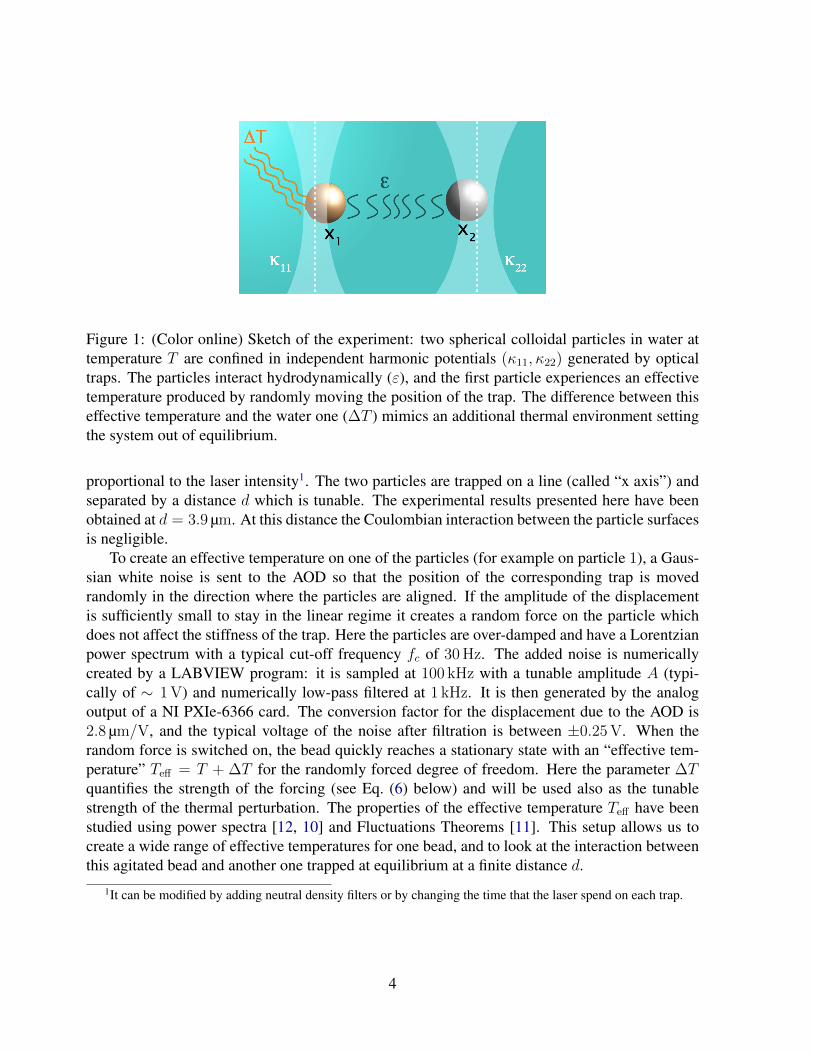
Figure 1: (Color online) Sketch of the experiment: two spherical colloidal particles in water attemperature T are confined in independent harmonic potentials (κ11, κ22) generated by opticaltraps. The particles interact hydrodynamically (ε), and the first particle experiences an effectivetemperature produced by randomly moving the position of the trap. The difference between thiseffective temperature and the water one (∆T ) mimics an additional thermal environment settingthe system out of equilibrium.
proportional to the laser intensity1. The two particles are trapped on a line (called “x axis”) andseparated by a distance d which is tunable. The experimental results presented here have beenobtained at d = 3.9 µm. At this distance the Coulombian interaction between the particle surfacesis negligible.
To create an effective temperature on one of the particles (for example on particle 1), a Gaus-sian white noise is sent to the AOD so that the position of the corresponding trap is movedrandomly in the direction where the particles are aligned. If the amplitude of the displacementis sufficiently small to stay in the linear regime it creates a random force on the particle whichdoes not affect the stiffness of the trap. Here the particles are over-damped and have a Lorentzianpower spectrum with a typical cut-off frequency fc of 30 Hz. The added noise is numericallycreated by a LABVIEW program: it is sampled at 100 kHz with a tunable amplitude A (typi-cally of ∼ 1 V) and numerically low-pass filtered at 1 kHz. It is then generated by the analogoutput of a NI PXIe-6366 card. The conversion factor for the displacement due to the AOD is2.8 µm/V, and the typical voltage of the noise after filtration is between ±0.25 V. When therandom force is switched on, the bead quickly reaches a stationary state with an “effective tem-perature” Teff = T + ∆T for the randomly forced degree of freedom. Here the parameter ∆Tquantifies the strength of the forcing (see Eq. (6) below) and will be used also as the tunablestrength of the thermal perturbation. The properties of the effective temperature Teff have beenstudied using power spectra [12, 10] and Fluctuations Theorems [11]. This setup allows us tocreate a wide range of effective temperatures for one bead, and to look at the interaction betweenthis agitated bead and another one trapped at equilibrium at a finite distance d.
1It can be modified by adding neutral density filters or by changing the time that the laser spend on each trap.
4

2 TheoryLet us consider a system with N degrees of freedom, whose state is a vector denoted by x ≡(x1, x2, . . . , xN). We write the equation of motion of our overdamped system in matrix notationas
x = a(x) +Bξ , (1)
where the vector a(x) is the mean drift velocity, and the N ×N matrix B is the noise amplitude,which is assumed to be independent of the state x. The differential noise ξ(t) is Gaussian andcolorless as well as uncorrelated among different components, i.e., 〈ξi(t)ξj(s)〉 = δijδ(t − s).Explicit time dependences of x, ξ, and possibly a andB, are omitted for simplifying the notation,except for occasions when emphasis is appropriate. Furthermore, as has already been hinted at,we will alternate between matrix and index notations according to whichever is more intelligiblein specific situations.
As an example, the drift vector of a hydrodynamic system is given in terms of the determin-istic force F (x) and of the mobility matrix µ,
a(x) = µF (x) . (2)
Due to hydrodynamic interactions, the mobility matrix has nonvanishing off-diagonal entriesµij 6= 0 that couple different degrees of freedom i 6= j. In general this would result in a state-dependent mobility, since the coupling depends on the difference of coordinates. However, we areconcerned with an experiment where a state-independent mobility is a viable approximation: Thehydrodynamic coupling between distant degrees of freedom is in the form of a series expansionin the ratio of particle radius to distance [25]. Hence, if the system is maintained such that theaverage distance is considerably larger than its fluctuations, it can be assumed to remain constantat its average value to lowest order. The optical traps in the considered experimental setup are“stiff” enough to achieve just that. The resulting mobility matrix, to the aforementioned level ofapproximation, for this system with N = 2 is given as
µ =1
γ
[1 εε 1
], (3)
where ε = 3R/2d is a small hydrodynamic coupling between spherical colloids of radius Rseparated by a(n average) distance d according to the Oseen approximation (ε = 0.2766 in theexperiment we consider), and γ =16.8 pNms/µm is the drag coefficient of the colloids in wa-ter. The distance d is set by the separation of the two harmonic optical traps, whose associatedpotential energy is
U(x) = 12x†κx , (4)
when each coordinate is measured with respect to the center of its corresponding trap, where κ isa diagonal matrix of stiffness constants. We thus have a stochastic system with linear forces; seee.g. [56, 22] for some recent results on this kind of systems.
5
As a result of the form of the mobility matrix, the diffusivity
D = 12BB† (5)
is also endowed with nonvanishing off-diagonal entries that are state-independent. In fact, in thegiven experimental setup, the diffusivity is a sum of two contributions [57]
D = Tµ+ ∆Tµ
[γ 00 0
]µ =
1
γ
[T + ∆T ε(T + ∆T )ε(T + ∆T ) T + ε2∆T
], (6)
the first of which originates from the solvent at temperature T , and the second from the stochasticforcing on particle 1, which has a white power spectrum of magnitude γ∆T [12].
2.1 Thermal perturbation and change of variablesOur aim is to investigate the response of the system to a small variation in its diffusion matrix,which is the most direct analog of temperature in this multidimensional situation. However, it isbetter to begin the treatment in terms of the noise amplitude, which is less physical, and revert todiffusivity at an appropriate stage.
We begin by perturbing the noise prefactor matrix as,
B(t) = B + δB(t) , (7)
and then follow the technique of Ref. [27], which is unfettered by terms that depend on the timediscretization. To this end, we change variables by defining
x(t) = B(t)B−1x(t) , (8)
which implies
x = BB−1 ˙x+ δBB−1x . (9)
Plugging this into the equation of motion (1), and multiplying it by BB−1 from the left, one has
˙x = −BB−1δBB−1x+ BB−1a(x) + Bξ
= −δBB−1x+ BB−1a(x) + Bξ , (10)
to first order in δB. Before proceeding with the simplification any further, one sees that thewhole point of this exercise was to rid the noise process of its perturbed prefactor, and make theperturbation appear elsewhere.
Note the argument x, rather than x, of a(x) in Eq. (10). In order to arrive at an equation ofmotion for the coordinate x, we therefore have to expand:
ai(x) = ai(x) + (xj − xj)∂ai(x)
∂xj
= ai(x) +(δBB−1x
)j
∂ai(x)
∂xj, (11)
6
where a summation is implied over repeated indices, and the difference x−xwas given by Eq. (8).Noting also that B−1 = B−1 − B−1δBB−1 to first order, we can proceed with the simplificationof Eq. (10) to find
˙xi =(
1− δBB−1)ij
[aj(x) +
(δBB−1x
)k
∂aj(x)
∂xk
]− (δBB−1x)i + Bijξj , (12)
or after discarding terms of order higher than 1 in δB,
˙xi = ai(x)− (δBB−1)ijaj(x) +(δBB−1x
)k
∂ai(x)
∂xk− (δBB−1x)i + Bijξj . (13)
We see that it is convenient to define
h(t) = δB(t)B−1 , (14)
which is a dimensionless smallness parameter matrix. After the convenience of this parameter isduly exploited, it will be rewritten in terms of the diffusivity rather than the noise prefactor.
Finally, we can rearrange Eq. (13) into
˙x = a(x) + Bξ (15)
where
a(x) = a(x) + α(x) , (16)
αi(x) = −hikak(x) + hklxl∂ai(x)
∂xk− hikxk , (17)
with h = δBB−1 according to Eq. (14). Thus, the perturbation of the noise prefactor in theevolution of x has been re-expressed as a perturbation of the mechanical force in the evolution ofx. Ref. [26] discusses another perspective from which this deformation of a thermal perturbationinto a deterministic perturbation can be viewed. Note that the “pseudo-force” α(x(t); t) dependsexplicitly on time through the perturbation h(t).
2.2 Path weight and responseThe objective of linear response is to investigate the variation of the expectation value of anobservable to linear order in a small perturbation. Taking the observable to be a state observable,O(t) = O(x(t)), this variation has the form
δ〈O(t)〉 = 〈O(t)δ lnP [x]〉 , (18)
due simply to the variation of the probability weights, P [x], of trajectories x(t). The negativelogarithm of the path weight,
− lnP [x] = A[x] , (19)
7

is commonly termed the path action. However, let us remark and remind that due to technicaldifficulties of varying the action with respect to noise amplitude, we will utilize the coordinate xwhich, as discussed earlier, reformulates the problem in terms of a variation of the deterministicforce.
According to the equation of motion (15) for x(t) with the Gaussian noise process ξ(t), theprobability weight of a trajectory x(t) has the quadratic action
A[x] =
∫ds
4
[˙xi − ai(x)
]D−1ij
[˙xj − aj(x)
]+
∫ds
2
∂
∂xiai(x) (20)
in the Stratonovich convention [58] up to a trajectory-independent additive constant, and thesymmetric matrix 2D = BB†.2 Also note that evaluation of the integrands at time s is implied.
The variation of Eq. (20) to first order in α(x) is simply
δA[x] = −∫
ds
2
[D−1ij
(˙xj − aj
)− ∂
∂xi
]αi(x(s); s) . (21)
Note that due to its definition (17), α(x) is of at least first order in the perturbation parameterh(s). Thus, the replacement (x, D) → (x,D) incurs errors only of orders which are alreadytruncated in this linear response scheme. That is to say, in Eq. (18) one can use δ lnP [x] =−δA[x] = −δA[x] via (x, D) → (x,D) in Eq. (21). Using Eq. (17) to express α(x) explicitly,we rewrite
δA[x] = −∫
ds
2
[D−1ij (xj − aj)− ∂i
] (−hikak + hklxl∂kai − hikxk
), (22)
where ∂i is shorthand for ∂/∂xi. Here, one can count powers of time derivative (dots on x or h)to determine the parity of each term under time-reversal, which is relevant for thermodynamicalarguments. Labeling according to the parity (−/+) under time-reversal, we separate δA[x] into3
δA−[x] = −∫
ds
2
[D−1ij xj(hklxl∂kai − hikak) + hikxkD
−1ij aj + hkk
], (22a)
and
δA+[x] = −∫
ds
2D−1ij aj(hikak − hklxl∂kai) +
∫ds
2(hklxl∂k∂iai +D−1
ij xjhikxk) , (22b)
with δA[x] = δA+[x] + δA−[x]. Via integration by parts, h(s) can be exchanged with h(s).4
After also manipulating the indices for the convenience of isolating a common factor, hkl(s), one
2For brevity of notation, we denote the elements of the inverse of a matrix as inD−1ij rather than the unambiguous
but cumbersome (D−1)ij .3Note that ∂i(hklxl∂kai − hikak) = hklxl∂k∂iai + hklδil∂kai − hik∂iak = hklxl∂k∂iai.4For this matter, we note here that we have intentionally left out integration limits in the action: The forcing h(s)
is assumed to be temporally localized, and the integration domain is infinite in principle. Thus,∫ds hg = −
∫ds hg
for a generic function g(s), and likewise∫ds hkk = 0 in Eq. (22a).
8
has
δA−[x] = −∫
ds
2
[D−1ij xjxl∂kai −D−1
kj (xjal + xlaj)−D−1kj xixl∂iaj
]hkl , (23a)
δA+[x] = −∫
ds
2
[D−1kj ajal −D
−1ij ajxl∂kai − xl∂k∂iai +D−1
kjdds
(xjxl)]hkl , (23b)
where the identity aj = xi∂iaj was used in (d/ds)(xlaj) = xlaj + xlaj , owing to Stratonovichcalculus, concerning the very last term.
Up until now, we have not elaborated about the dimensionless parameter matrix h(s), whichwe do in Appendix B. The gist is that, rather than expressing h(s) via the somewhat nonphysicalnoise prefactor B via Eq. (14), one can write it in terms of the variation of the inverse diffusivity,δD−1, which is a more sensible physical quantity. The manifest symmetry in the contents ofthe resulting expression, h = (−1/2)DδD−1, facilitates certain simplifications on δA[x]. Inparticular, now that D−1
jk hkl = (−1/2)δD−1jl is a symmetric matrix, the last term of Eq. (23b) can
benefit from
D−1kj hkl
dds
(xjxl) = −12δD−1
jldds
(xjxl) = −14δD−1
jld2
ds2(xjxl) . (24)
Similarly, the two middle terms of Eq. (23a) combine. With these simplifications we finally have
δA−[x] =
∫ds xi
4
[(D−1ij Dkm − δikδjm
)xl∂kaj − 2δimal
]δD−1
ml , (25a)
δA+[x] =
∫ds
4
[amal −Dkmxl
(D−1ij aj∂kai + ∂k∂iai
)+ 1
2d2
ds2(xmxl)
]δD−1
ml . (25b)
At this stage, it would be possible to define a tensorial response function for a state observableO(t) = O(x(t)) to an impulsive variation in the inverse diffusivity matrix as
Rlm(t, s) = −⟨O(x(t))
δA[x]
δD−1lm (s)
⟩, (26)
which satisfies δ〈O(t)〉 = −〈O(t)δA[x]〉 =∫
dsRlm(t, s)δD−1lm (s), yielding
Rlm(t, s) ≡ R−lm(t, s) +R+lm(t, s) (27)
with
R−lm(t, s) = −⟨O(t)
4
[(D−1ij Dkm − δikδjm
)xixl∂kaj − 2xmal
](s)
⟩, (27a)
R+lm(t, s) = −
⟨O(t)
4
[amal −Dkmxl
(D−1ij aj∂kai + ∂k∂iai
)+ 1
2d2
ds2(xmxl)
](s)
⟩. (27b)
These expressions are the generalization of those of Refs. [27, 26] to non-negligible state-independenthydrodynamic coupling. Note the “collective” argument (s) that applies to all the time depen-dence inside the square brackets preceding it.
9

2.3 Stationary susceptibilityThe integrated response is called susceptibility. In practice, one is usually able to manipulate asingle scalar parameter, call it λ(s). It suits to write the variation δD−1
lm (s) in terms of the variationδλ(s) of the parameter (to first order): δD−1
lm (s) = δλ(s)(∂D−1lm/∂λ). Then, an empirically
accessible susceptibility to a stepwise change in λ at t = 0 can be expressed as
χ(t) =∂ 〈O(t)〉λ
∂λ
∣∣∣∣∣λ=λ(0)
=
∫ t
0
dsHlmRlm(t, s) , (28)
with
Hlm ≡∂D−1
lm
∂λ
∣∣∣∣λ=λ(0)
. (29)
The time integral of Eq. (28) removes one of the derivatives d/ds in the last term of Eq. (27b)and gives the boundary term,
−⟨O(t)1
8dds
[xm(s)xl(s)]∣∣t0
⟩. (30)
The remaining derivative can also be removed if we specialize to the case where the initial distri-bution ρ(x(0)) in the unperturbed averages 〈·〉 is stationary, since, due to invariance under timetranslation, the response function becomesR(t, s) = R(t− s), and in particular
−⟨O(t)1
8dds
[xm(s)xl(s)]∣∣t0
⟩=⟨
18
dO(t)dt
[xm(s)xl(s)]∣∣t0
⟩. (31)
The time derivative at the later instant t can then be replaced by the backward generator of thedynamics, i.e., ⟨
18
dO(t)dt
[xm(s)xl(s)]∣∣t0
⟩=⟨
18LO(t)[xm(s)xl(s)]
∣∣t0
⟩, (32)
where
L = ai∂i +Dij∂i∂j . (33)
This replacement is desirable, because the original expression on the left-hand side of Eq. (32)with the time derivative is much noisier, and thus requires much more statistics to converge. Sinceour application will be in a the stationary state, we take advantage of this and continue from hereon with the assumption of stationarity.
As previously done [26], we split the susceptibility into four terms
χ(t) = χ−1 (t) + χ−2 (t) + χ+1 (t) + χ+
2 (t) , (34)
10

where
χ−1 (t) =1
2
∫ t
0
dsHml 〈O(t)[xmal](s)〉 , (34a)
χ−2 (t) =1
4
∫ t
0
dsHml
⟨O(t)[(δikδjm −D−1
ij Dkm)xixl∂kaj](s)⟩, (34b)
χ+1 (t) =
1
4
∫ t
0
dsHml
⟨O(t)[xlDkmD
−1ij aj∂kai − amal](s)
⟩, (34c)
χ+2 (t) =
1
8Hml
⟨LO(t)xm(s)xl(s)
∣∣t0
⟩. (34d)
are written in terms of Stratonovich stochastic integrals. If the heat bath is in equilibrium, the termχ−1 (t) corresponds to the correlation between the observable and half of the entropy production inthe bath. This interpretation, previously discussed for the linear response to mechanical forces [6,7] and temperature variations [3, 27, 26], is not possible in our experiment and we remain with thefact that χ−1 (t) as well as χ−2 (t) correlate the observable with time-antisymmetric, i.e., entropy-production-like quantities. The correlations in χ+
1 (t) and χ+2 (t) instead involve time-symmetric,
non-dissipative variables. They were named “frenetic” terms because often those time-symmetricobservables quantify how agitated, or frenzied, is the exploration of the system state space [6, 7,5].
2.4 Susceptibility in matrix notationDespite the many indices appearing in Eq. (34), note that the highest rank tensor involved aboveis still of rank two. Therefore, the index contractions can be broken up into ordinary matrixoperations. This should be useful, for example, for a numerical implementation in a softwarewhere matrix multiplication is defined.
We denote by ∇a† the matrix with elements ∂iaj (where i is the row index). Thus, we dealwith vectors (the positions x, velocities x, and drifts a) and matrices. The latter are the noisevariation H (defined in Eq. (29)), the diffusivity matrix D and its inverse D−1, and ∇a†. Bysimply following the sequence of index repetitions, it is straightforward to express the terms inthe susceptibility as
χ−1 (t) =1
2
∫ t
0
ds⟨O(t)[x†Ha](s)
⟩, (35a)
χ−2 (t) =1
4
∫ t
0
ds⟨O(t)[x†(∇a†)Hx− x†HD(∇a†)D−1x](s)
⟩, (35b)
χ+1 (t) =
1
4
∫ t
0
ds⟨O(t)[x†HD(∇a†)D−1a− a†Ha](s)
⟩, (35c)
χ+2 (t) =
1
8
⟨LO(t) [x†Hx](s)
⟩ ∣∣s=ts=0
. (35d)
If the stationary conditions are not satisfied, the last term should be evaluated as
χ+2 (t) = −1
8
d
ds
⟨O(t) [x†Hx](s)
⟩ ∣∣s=ts=0
. (35e)
11

3 Susceptibility of the colloidal systemWe calculate the susceptibility of the colloidal system to a change in the effective temperature ofthe stochastic driving. We thus identify λ = ∆T and with Eq. (6) we find
H =∂(D−1)
∂∆T=
[ −γ(T+∆T )2
0
0 0
]. (36)
Using this expression in Eq. (28) via the response functions (27a)–(27b) along with the simplifi-cations sketched above, we find the susceptibility. Note that the term of the time-symmetric part(27b) proportional to ∂k∂iai, while in general nonzero, disappears for the particular system inquestion, since two derivatives of the mean drift a = µF = −µκx vanish due to the quadraticpotential (4).
Experimental data were sampled at constant rate, with a time step ∆t. This means that atrajectory is a discrete collection of points x(0), x(1), x(2), . . . , x(n) with n = t/∆t. For eachtemperature we have a long time series composed of ns = 106 samples, out of which we extractns−n+1 trajectories by shifting the initial point. Thus, these trajectories are partially overlappedwith other ones. Since the autocorrelation time of the system is about γ/κ11 ≈ γ/κ22 ≈ 5ms= 4∆t, we have taken the correlation of data into account by amplifying the error bars in ourresults (standard deviations) by a factor of
√4 = 2.
Velocities are defined as x(i) = [x(i + 1) − x(i)]/∆t. The integrals in Eq. (34) or Eq. (35)follow the Stratonovich convention. In their time-discretized version, quantities (other than thex mentioned above) in the integrals are averaged over time steps. For example, the average[x(i+ 1) + x(i)]/2 represents the positions at time step i.
To visualize the linear response of some observables, we start by considering the total energyU = κ11
2x2
1+κ222x2
2. The susceptibility of the energy can be considered a generalized heat capacity.In Figure 2 this susceptibility χ is plotted as a function of time for four cases: ∆T = 0 K,which is the equilibrium condition with no forcing on particle 1, and ∆T = 120 K, 340.8 K,and ∆T = 967.8 K, which become progressively farther from equilibrium. In equilibrium onecan notice that twice the entropic term χ−1 (which by definition is half of the Kubo formula forequilibrium systems), would be sufficient to obtain the susceptibility. This picture breaks downout of equilibrium, where it is the whole sum of the four components that yields the correct formof the susceptibility. For comparison, we show also the estimate χρ(t) obtained with the approachby Seifert and Speck [51], through
χρ(t) =
⟨O(t)
[∂ ln ρ(x(t))
∂∆T− ∂ ln ρ(x(0))
∂∆T
]⟩, (37)
which is an integrated version of their response formula. Appendix A sketches how the stationarydistribution ρ(x) for this system was computed. Figure 2 shows that the susceptibilities evaluatedwith the two approaches are compatible with each other.
As a second example, we show the susceptibility to a change of ∆T of the energy U2 = κ222x2
2
of the second particle, namely the colloid which is not experiencing the random forcing directly.Yet, due to the hydrodynamic interaction, its energy on average increases with ∆T , as manifested
12
∆T = 0 K ∆T = 120 K
0 5 10 15 20 25 30time [ms]
-0.1
0
0.1
0.2
0.3
0.4
0.5
χχ
1-
χ2-
χ1
+
χ2
+
χρ
0 5 10 15 20 25 30time [ms]
-0.1
0
0.1
0.2
0.3
0.4
0.5
χχ
1-
χ2-
χ1
+
χ2
+
χρ
∆T = 340.8 K ∆T = 967.8 K
0 5 10 15 20 25 30time [ms]
-0.1
0
0.1
0.2
0.3
0.4
0.5
χχ
1-
χ2-
χ1
+
χ2
+
χρ
0 5 10 15 20 25 30time [ms]
-0.1
0
0.1
0.2
0.3
0.4
0.5
χχ
1-
χ2-
χ1
+
χ2
+
χρ
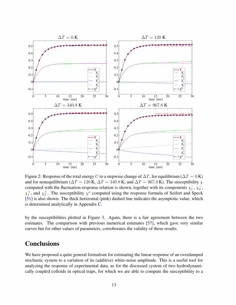
Figure 2: Response of the total energyU to a stepwise change of ∆T , for equilibrium (∆T = 0 K)and for nonequilibrium (∆T = 120 K, ∆T = 340.8 K, and ∆T = 967.8 K). The susceptibility χcomputed with the fluctuation-response relation is shown, together with its components χ−1 , χ−2 ,χ+
1 , and χ+2 . The susceptibility χρ computed using the response formula of Seifert and Speck
[51] is also shown. The thick horizontal (pink) dashed line indicates the asymptotic value, whichis determined analytically in Appendix C.
by the susceptibilities plotted in Figure 3. Again, there is a fair agreement between the twoestimates. The comparison with previous numerical estimates [57], which gave very similarcurves but for other values of parameters, corroborates the validity of these results.
ConclusionsWe have proposed a quite general formalism for estimating the linear response of an overdampedstochastic system to a variation of its (additive) white-noise amplitude. This is a useful tool foranalyzing the response of experimental data, as for the discussed system of two hydrodynami-cally coupled colloids in optical traps, for which we are able to compute the susceptibility to a
13

∆T = 0 K ∆T = 120 K
0 5 10 15 20 25 30time [ms]
-0.01
0
0.01
0.02
χχ
1-
χ2-
χ1
+
χ2
+
χρ
0 5 10 15 20 25 30time [ms]
-0.01
0
0.01
0.02
χχ
1-
χ2-
χ1
+
χ2
+
χρ
∆T = 340.8 K ∆T = 967.8 K
0 5 10 15 20 25 30time [ms]
-0.01
0
0.01
0.02
χχ
1-
χ2-
χ1
+
χ2
+
χρ
0 5 10 15 20 25 30time [ms]
-0.01
0
0.01
0.02
χχ
1-
χ2-
χ1
+
χ2
+
χρ
Figure 3: Response of the energy U2 of the second particle to a stepwise change of ∆T , see thelegend of Figure 2 for all the details.
change of an external random driving that reproduces a sort of higher temperature for only oneof the colloids. Yet, note that our formalism if quite flexible and can be applied to more ab-stract stochastic diffusive dynamics with correlated noise. The next evolution of this approachshould try to complete the picture by dealing with systems with multiplicative noise. Also thethermal response for nonequilibrium inertial systems should be developed without resorting tothe time-discretization used in a previous work [3]. This would allow, for example, to determinenonequilibrium steady-state thermal susceptibilities of the Fermi-Pasta-Ulam model [39, 24] orother Hamiltonian models of heat conduction.
Similarly to the linear response of nonequilibrium systems to mechanical perturbations, wenote that the susceptibility to temperature changes arises from dissipative as well as non-dissipativeaspects of the dynamics. This differs from the simple structure of response theory for equilibriumsystems, where only correlations between heat fluxes (i.e., dissipation) and observable are rele-vant for computing susceptibilities. With these considerations in mind, the kind of fluctuation-response relations we discussed might be used to better understand and quantify the thermalresponse of nonequilibrium systems such as relaxing glasses [8, 40, 16, 43, 21] and active mat-
14
ter [43, 41, 30, 45].
Appendices
A Stationary distributionHere we briefly sketch the calculation of the stationary distribution of the system, for the sake ofcompleteness.
With a drift a(x) = −µκx linear in x, the equation of motion (1) describes an Ornstein-Uhlenbeck process, which we rewrite here as
x = −Ωx+√
2Dξ , (38)
with Ω = µκ. According to the corresponding Fokker-Planck equation, ρ = −∂iJi, stationarityrequires the ensemble current J = −ρΩx−D∇ρ to be divergenceless, yielding
0 = ρΩii + Ωijxj∂iρ+Dij∂i∂jρ . (39)
Clearly, a Gaussian distribution of the form
ρ(x) = Z−1e−12x†Gx (40)
satisfies the zero divergence condition above. To find the inverse covariance matrix G, one sub-stitutes the ansatz, upon which a few lines of algebra implies the condition
ΩG−1 +G−1Ω† = 2D . (41)
This is a system of linear equations in the elements of the covariance matrix G−1, which can besolved, for instance, by rewriting it in terms of a vector composed of the columns of G−1. Here,we simply quote the resulting matrix: Recalling Ω = µκ with κ diagonal and µ given in Eq. (3),and D given in Eq. (6), one finds
G−1 =
[T+(1−ε2)∆T
κ11+ ε2∆T
κ11+κ22ε∆T
κ11+κ22ε∆T
κ11+κ22Tκ22
+ ε2∆Tκ11+κ22
]. (42)
Inversion of this matrix thus determines the stationary distribution (40).
B Form of the perturbation parameterEven though it may sometimes be more convenient mathematically to work in terms of the noiseamplitude B, it is the diffusivity matrix D which is physically relevant, since the noise amplitudeis fixed only up to an orthogonal transformation. Hence the perturbation parameter, h = δBB−1,defined in Sec. 2.1 in terms of the noise amplitude should eventually be expressed in terms of a
15

perturbation of the diffusivity. With D = D + δD and B = B + δB, in line with Sec. 2.1, thedefinitions 2D = BB† and 2D = BB† imply that
2δD = BδB† + δBB† . (43)
Note that one should not expect to solve this equation for δB uniquely given a specific δD; manynoise coefficient matrices B map into the same diffusion matrix D.
The relation above can now be used to express the perturbation parameter h = δBB−1 interms of D and δD, but not uniquely, which is not a problem. Multiplying Eq. (43) by D−1 fromthe left and right, one easily finds
D−1δDD−1 = D−1h+ h†D−1 . (44)
The left hand side of this equation is equal to −δD−1 (verified easily by varying the identity1 = DD−1) which is determined by the physical description of the perturbation. Meanwhile,the right hand side of the equation is twice the symmetric part of D−1h. In other words, it isonly the symmetric part of D−1h that is fixed by the physical form of the perturbation, and theantisymmetric part is left undetermined. It therefore behooves one to choose D−1h to be purelysymmetric, whence one obtains −δD−1 = 2D−1h, or
h = −12DδD−1 = −1
2DδD−1 , (45)
where the second equality is valid due to the overarching first order approximation of linearresponse.
C Asymptotic values of the susceptibilityIn this appendix, we sketch how the asymptotic values for the susceptibilities in Figures 2 and 3were obtained.
One can derive a host of relations valid in the stationary regime by requiring that time deriva-tives of state observables vanish [28]. For the present discussion, the relevant observable is thetensor xixj , i.e.,
0 =d
dt〈xixj〉 = 〈Lxixj〉 , (46)
with the backward generator L = ai∂i +Dij∂i∂j . (One should keep in mind that the average is inthe stationary regime, although we leave it unlabeled.) When evaluated explicitly, with a = µF ,one finds the relation
0 = µ⟨Fx†
⟩+⟨xF †
⟩µ+ 2D . (47)
This matrix relation entails a set of equations for the independent components of the tensor〈xiFj〉, of which there are 3 in our case with 2 degrees of freedom.
16
We note that for our system, U(x) = −(1/2)Tr(Fx). Thus, multiplying Eq. (47) from theleft by µ−1 and taking the trace, we find the stationary average of the potential energy to be
〈U(x)〉 = −1
2Tr 〈Fx〉 =
1
2Tr(µ−1D) . (48)
Hence, the stationary (asymptotic) value for the susceptibility is found as
∂ 〈U〉∂∆T
=1
2Tr
(µ−1 ∂D
∂∆T
)=
1
2, (49)
which was evaluated using Eq. (6) for the diffusion matrix. This asymptotic value for χ wasindicated in Figure 2.
The susceptibility of the energy of the second particle U2(x2) = −(1/2)F2x2 can be extractedsimilarly from Eq. (47), with the exception that one has to go through the tedium of actuallysolving for the component 〈F2x2〉. We quote only the result of this straightforward exercise:
∂ 〈U2〉∂∆T
=− 1
2
∂
∂∆T〈F2x2〉 =
ε2
2(
1 + κ11κ22
) . (50)
This was evaluated as 0.01899 for the actual experimental values of κ11 = 3.3745 pN/µm,κ22 = 3.3285 pN/µm, and ε = 0.2766, and indicated in Figure 3 as the asymptotic value ofthe susceptibility χ.
References[1] Agarwal, G.S.: Fluctuation-dissipation theorems for systems in non-thermal equilibrium
and applications. Z. Physik 252, 25–38 (1972)
[2] Altaner, B., Polettini, M., Esposito, M.: Fluctuation-dissipation relations far from equilib-rium. Phys. Rev. Lett. 117, 180601 (2016)
[3] Baiesi, M., Basu, U., Maes, C.: Thermal response in driven diffusive systems. Eur. Phys. J.B 87, 277 (2014)
[4] Baiesi, M., Ciliberto, S., Falasco, G., Yolcu, C.: Thermal response of nonequilibrium RCcircuits. Phys. Rev. E 94, 022144 (2016)
[5] Baiesi, M., Maes, C.: An update on the nonequilibrium linear response. New J. Phys. 15,013004 (2013)
[6] Baiesi, M., Maes, C., Wynants, B.: Fluctuations and response of nonequilibrium states.Phys. Rev. Lett. 103, 010602 (2009)
[7] Baiesi, M., Maes, C., Wynants, B.: Nonequilibrium linear response for Markov dynamics,I: Jump processes and overdamped diffusions. J. Stat. Phys. 137, 1094–1116 (2009)
17

[8] Barrat, J.L., Kob, W.: Fluctuation-dissipation ratio in an aging Lennard-Jones glass. Euro-phys. Lett. 46, 637–642 (1999)
[9] Bertini, L., Gabrielli, D., Jona-Lasinio, G., Landim, C.: Clausius inequality and optimalityof quasistatic transformations for nonequilibrium stationary states. Phys. Rev. Lett. 114,020601 (2013)
[10] Bérut, A., Imparato, A., Petrosyan, A., Ciliberto, S.: The role of coupling on the statisticalproperties of the energy fluxes between stochastic systems at different temperatures. J. Stat.Mech., P054002 (2016)
[11] Bérut, A., Imparato, A., Petrosyan, A., Ciliberto, S.: Stationary and transient fluctuationtheorems for effective heat fluxes between hydrodynamically coupled particles in opticaltraps. Phys. Rev. Lett. 116, 068301 (2016)
[12] Bérut, A., Petrosyan, A., Ciliberto, S.: Energy flow between two hydrodynamically coupledparticles kept at different effective temperatures. Europhys. Lett. 107, 60004 (2014)
[13] Bohec, P., Gallet, F., Maes, C., Safaverdi, S., Visco, P., van Wijland, F.: Probing activeforces via a fluctuation-dissipation relation: Application to living cells. Europhys. Lett.102, 50005 (2013)
[14] Boksenbojm, E., Maes, C., Netocný, K., Pešek, J.: Heat capacity in nonequilibrium steadystates. Europhys. Lett. 96, 40001 (2011)
[15] Brandner, K., Saito, K., Seifert, U.: Thermodynamics of micro- and nano-systems drivenby periodic temperature variations. Phys. Rev. X 5, 031019 (2016)
[16] Cammarota, C., Cavagna, A., Gradenigo, G., Grigera, T.S., Verrocchio, P.: Numerical de-termination of the exponents controlling the relationship between time, length, and temper-ature in glass-forming liquids. J. Chem. Phys. 131, 194901 (2009)
[17] Chetrite, R.: Fluctuation relations for diffusion that is thermally driven by a nonstationarybath. Phys. Rev. E 80, 051107 (2009)
[18] Chetrite, R., Falkovich, G., Gawedzki, K.: Fluctuation relations in simple examples of non-equilibrium steady states. J. Stat. Mech., P08005 (2008)
[19] Ciliberto, S., Imparato, A., Naert, A., Tanase, M.: Heat flux and entropy produced bythermal fluctuations. Phys. Rev. Lett. 110, 180601 (2013)
[20] Ciliberto, S., Imparato, A., Naert, A., Tanase, M.: Statistical properties of the energy ex-changed between two heat baths coupled by thermal fluctuations. J. Stat. Mech., P12014(2013)
[21] Crisanti, A., Picco, M., Ritort, F.: Fluctuation Relation for Weakly Ergodic Aging Systems.Phys. Rev. Lett. 110, 080601 (2013)
18

[22] Crisanti, A., Puglisi, A., Villamaina, D.: Non-equilibrium and information: the role ofcross-correlations. Phys. Rev. E 85, 061127 (2012)
[23] Cugliandolo, L., Kurchan, J., Parisi, G.: Off equilibrium dynamics and aging in unfrustratedsystems. J. Phys. I 4, 1641 (1994)
[24] Dhar, A.: Heat transport in low-dimensional systems. Adv. Phys. 57, 457–537 (2008)
[25] Doi, M., Edwards, S.: The Theory of Polymer Dynamics. International series of mono-graphs on physics. Clarendon Press (1988)
[26] Falasco, G., Baiesi, M.: Nonequilibrium temperature response for stochastic overdampedsystems. New J. Phys. 18, 043039 (2016)
[27] Falasco, G., Baiesi, M.: Temperature response in nonequilibrium stochastic systems. Euro-phys. Lett. 113, 20005 (2016)
[28] Falasco, G., Baldovin, F., Kroy, K., Baiesi, M.: Mesoscopic virial equation for nonequilib-rium statistical mechanics. New J. Phys. 18, 093,043 (2016)
[29] Falcioni, M., Isola, S., Vulpiani, A.: Correlation functions and relaxation properties inchaotic dynamics and statistical mechanics. Phys. Lett. A 144, 341 (1990)
[30] Gautrais, J., Ginelli, F., Fournier, R., Blanco, S., Soria, M., Chate, H., Theraulaz, G.: Deci-phering Interactions in Moving Animal Groups. PLoS Comp. Biol. 8, e1002678 (2012)
[31] Girsanov, I.V.: On transforming a certain class of stochastic processes by absolutely contin-uous substitution of measures. Theor. Probab. Applic. 5(3), 285–301 (1960)
[32] Gomez-Solano, J.R., Petrosyan, A., Ciliberto, S.: Fluctuations, linear response and heatflux of an aging system. Europhys. Lett. 98, 10007 (2012)
[33] Gomez-Solano, J.R., Petrosyan, A., Ciliberto, S., Chetrite, R., , Gawedzki, K.: Experimen-tal verification of a modified fluctuation-dissipation relation for a micron-sized particle in anon-equilibrium steady state. Phys. Rev. Lett. 103, 040601 (2009)
[34] Gomez-Solano, J.R., Petrosyan, A., Ciliberto, S., Maes, C.: Fluctuations and response in anon-equilibrium micron-sized system. J. Stat. Mech., P01008 (2011)
[35] Hatano, T., Sasa, S.: Steady-state thermodynamics of Langevin systems. Phys. Rev. Lett.86, 3463–3466 (2001)
[36] Kailath, T.: The structure of Radon-Nikodym derivatives with respect to Wiener and relatedmeasures. Ann. Math. Statist. 42(3), 1054–1067 (1971)
[37] Katz, S., Lebowitz, J.L., Spohn, H.: Phase transitions in stationary nonequilibrium states ofmodel lattice systems. Phys. Rev. B 28, 1655–1658 (1983)
19
[38] Komatsu, T.S., Nakagawa, N., Sasa, S., Tasaki, H.: Exact equalities and thermodynamicrelations for nonequilibrium steady states. J. Stat. Phys. 159, 1237–1285 (2015)
[39] Lepri, S., Livi, R., Politi, A.: Thermal conduction in classical low-dimensional lattices.Phys. Rep. 377, 1–80 (2003)
[40] Lippiello, E., Corberi, F., Zannetti, M.: Fluctuation dissipation relations far from equilib-rium. J. Stat. Mech., P07002 (2007)
[41] Loi, D., Mossa, S., Cugliandolo, L.F.: Non-conservative forces and effective temperaturesin active polymers. Soft Matt. 7, 10193–10209 (2011)
[42] Maes, C., Netocný, K.: A nonequilibrium extension of the Clausius heat theorem. J. Stat.Phys. 154, 188–203 (2014)
[43] Maggi, C., Di Leonardo, R., Dyre, J.C., Ruocco, G.: Generalized fluctuation-dissipationrelation and effective temperature in off-equilibrium colloids. Phys. Rev. B 81, 104201(2010)
[44] Mandal, D., Jarzynski, C.: Analysis of slow transitions between nonequilibrium steadystates. J. Stat. Mech., 063204 (2016)
[45] Marchetti, M.C., Joanny, J.F., Ramaswamy, S., Liverpool, T.B., Prost, J., Rao, M., AditiSimha, R.: Hydrodynamics of soft active matter. Rev. Mod. Phys. 85, 1143 (2013)
[46] Nakamura, T., Sasa, S.: A fluctuation-response relation of many Brownian particles undernon-equilibrium conditions. Phys. Rev. E 77, 021108 (2008)
[47] Oono, Y., Paniconi, M.: Steady state thermodynamics. Progr. Theor. Phys. Suppl. 130,29–44 (1998)
[48] Proesmans, K., Cleuren, B., Van den Broeck, C.: Linear stochastic thermodynamics forperiodically driven systems. J. Stat. Mech., 023202 (2016)
[49] Prost, J., Joanny, J.F., Parrondo, J.M.: Generalized fluctuation-dissipation theorem forsteady-state systems. Phys. Rev. Lett. 103, 090601 (2009)
[50] Sagawa, T., Hayakawa, H.: Geometrical expression of excess entropy production. Phys.Rev. E 84, 051110 (2011)
[51] Seifert, U., Speck, T.: Fluctuation-dissipation theorem in nonequilibrium steady states. Eu-rophys. Lett. 89, 10007 (2010)
[52] Sekimoto, K.: Microscopic heat from the energetics of stochastic phenomena. Phys. Rev. E76, 060103(R) (2007)
[53] Speck, T., Seifert, U.: Restoring a fluctuation-dissipation theorem in a nonequilibriumsteady state. Europhys. Lett. 74, 391–396 (2006)
20
[54] Speck, T., Seifert, U.: Extended fluctuation-dissipation theorem for soft matter in stationaryflow. Phys. Rev. E 79, 040102 (2009)
[55] Verley, G., Mallick, K., Lacoste, D.: Modified fluctuation-dissipation theorem for non-equilibrium steady states and applications to molecular motors. Europhys. Lett. 93, 10002(2011)
[56] Villamaina, D., Baldassarri, A., Puglisi, A., Vulpiani, A.: Fluctuation dissipation relation:how does one compare correlation functions and responses? J. Stat. Mech. P07024 (2009)
[57] Yolcu, C., Baiesi, M.: Linear response of hydrodynamically-coupled particles under anonequilibrium reservoir. J. Stat. Mech., 033209 (2016)
[58] Zinn-Justin, J.: Quantum field theory and critical phenomena, 4th edn. Clarendon Press,Oxford (2002)
21