a general relativity primer - iosr...

IOSR Journal of Applied Physics (IOSR-JAP)

e-ISSN: 2278-4861. Volume 5, Issue 6 (Jan. 2014), PP 06-31

www.iosrjournals.org

www.iosrjournals.org 6 | Page

A General Relativity Primer

Salvish Goomanee

King’s College London, Department of Physics, Strand, London, WC2R 2LS, UK

Abstract: In this paper, the underlying principles about the theory of relativity are briefly introduced and

reviewed. The mathematical prerequisite needed for the understanding of general relativity and of Einstein field

equations are discussed. Concepts such as the principle of least action will be included and its explanation

using the Lagrange equations will be given. Where possible, the mathematical details and rigorous analysis of

the subject has been given in order to ensure a more precise and thorough understanding of the theory of

relativity. A brief mathematical analysis of how to derive the Einstein’s field’s equations from the Einstein-

Hilbert action and the Schwarzschild solution was also given.

I. Introduction

Relativity theory is one of the pillars of theoretical physics, since its development by A. Einstein in the

beginning of the 20th

century it is considered as one of the most successful invention by the human mind. In this

paper I will be describing the various ideas which contribute to the elaboration of the theory of relativity. The

mathematics of relativity is very subtle and contains a lot of information however I found it very surprising how

it was not very difficult to understand. It will be assumed that one needs primarily a very good knowledge of

vector calculus and partial differential equations in order to be able to follow the ideas of general relativity

described in this paper at the beginning. As I will be describing the approaches to the general theory of

relativity, I will gradually do so by using more of differential geometry. What is very interesting with the theory

of relativity is that it is a topic where geometry has a very important place. This actually makes the equations

slightly less difficult to understand as they can easily be associated to the topology of curved space.

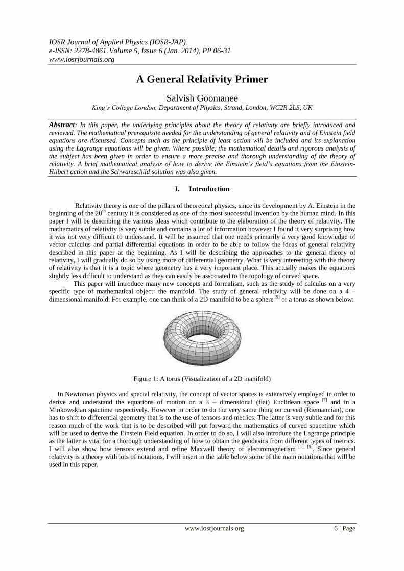
This paper will introduce many new concepts and formalism, such as the study of calculus on a very

specific type of mathematical object: the manifold. The study of general relativity will be done on a 4 –

dimensional manifold. For example, one can think of a 2D manifold to be a sphere [9]

or a torus as shown below:

Figure 1: A torus (Visualization of a 2D manifold)

In Newtonian physics and special relativity, the concept of vector spaces is extensively employed in order to

derive and understand the equations of motion on a 3 – dimensional (flat) Euclidean space [7]

and in a

Minkowskian spactime respectively. However in order to do the very same thing on curved (Riemannian), one

has to shift to differential geometry that is to the use of tensors and metrics. The latter is very subtle and for this

reason much of the work that is to be described will put forward the mathematics of curved spacetime which

will be used to derive the Einstein Field equation. In order to do so, I will also introduce the Lagrange principle

as the latter is vital for a thorough understanding of how to obtain the geodesics from different types of metrics.

I will also show how tensors extend and refine Maxwell theory of electromagnetism [1], [9]

. Since general

relativity is a theory with lots of notations, I will insert in the table below some of the main notations that will be

used in this paper.



A. Mathematical Notations for Relativity

where

Spacetime Coordinates (on manifold)

M

Spacetime (4D manifold)

∑

Einstein Summation Convention

f : M R where f F

F represents functions on manifold

Metric Tensor: It defines the scalar product between any

two vectors on M. It is non – positive definite meaning that it is Lorentzian.

(Largely employed in SR and GR).

Minkowski metric: The metric of special relativity used

in an inertial and Cartesian frame of reference. .

Greek Indices (

Denotes spacetime coordinates (From 0 to 3)

Latin Indices ( )

Denotes spatial component (From 1 to 3)

Table 1: Common notations and conventions used in special and general relativity theory.

There are even more notations present in the theory of general relativity due to the mathematics of

differential geometry which will be described later as doing so now will be meaningless. This is because many

of these notations should be properly understood in order to be fully defined. I now start by describing the

Lagrange formalism [4], [9]

and it various applications in theoretical physics which will be used further ahead.

II. The Lagrange Principle The Lagrange formalism was introduced by Joseph Louis Lagrange (1736 – 1813). This formulation

compared to the Newtonian system enables one to perform calculations involving vectors in a more general

coordinate system. This extension of the calculations is very important in general relativity. The Lagrange

formalism is important because of two main reasons. Firstly it holds in any coordinate system unlike the

Newton‟s equations which are valid only in an inertial frame of reference. Secondly it is easy to work with

constraints of Lagrangians. All fundamental principles of nature can be expressed in terms of a Lagrangian

density, L. Many are familiar with the Lagrangian density of the standard model in particle physics which

describes the broken symmetry due the Higgs field. The Lagrange method is a very effective if one wants to

obtain the equation of motion of a particle along the shortest path on a curved surface. In order to be able to

derive the Lagrange equations, one has to go through another very important principle, the principle of least

action. Just like the Lagrangian density is used to describe many physical principles so does the action principle

in a quite different way. It is present in general relativity as the Einstein – Hilbert action, in string theory and

many other theoretical principles of physics. The difficulty with this part of the paper is that one has to deal with

a lot of different notations and variables.

A. The Principle of Least Action

The Principle of Least action implies that the actual path taken by a system is an extremum of the action, S.

In order to proceed, one must make sure that all the notations being used are well defined as shown

below. I shall start with one of the basics of classical mechanics which are the Newton‟s equations. Consider

position of N particles with coordinates as , where A = 1, 2, 3 …, N described by equation (1)



(1)

where the dot represents derivative with respect to time, the number of degrees of freedom = 3N, as per

parameterization of a 3N dimensional space known as a configuration space, C. Curved path in C are described

by particle motion. With this defined, I shall now proceed to the definition of the Lagrangian, L. The latter is at

its simplest just a combination of the kinetic and potential energy of a system

(2)

where is the kinetic energy of the system and V(x) is the potential energy. The above equation will be

used in the definition of the action, S. In the principle of least action, the end points are fixed and of all possible

paths only one will be possible by the system – the extremum. And at the extremum will be 0. The method

used will involve calculus of variation. This is because as it will be shown, one will have to deal with a

functional (function of a function). The latter is not a function of a single variable.

The action is defined as

(3)

where the limits of the integration, ti and tf refer to initial and final time respectively. These end points are fixed

as mentioned previously, hence this implies that ( ) . I can consider a variation

in between the end points, this is shown below:

(4)

(5)

Now the second term is integrated by parts as shown below

. (6)

The term on the far right hand side will be 0 since end points are fixed and as is 0, one can see how the

Newton equation in (1) is recovered in a rather different form shown below:

(7)

(8)

Equation (8) is known as the Lagrange equation of the system, sometimes it is also referred to the Euler –

Lagrange equation. The above equation will used in some examples of classical mechanics and

electromagnetism in order to show how it applies to a given coordinate system. This will facilitate the

introduction of the Lagrange equation in deriving equation of motion in curved space. One may then ask, for a

given coordinate system, how the Lagrangian will behave in different frame of reference, will a Lagrangian

written in an x – frame of reference be different to that written in a y – frame of reference? The answer is no,



this is because the Lagrangian is symmetric. It is a property which will be used in the following example. This

example is a problem for which I have worked out the solution.

Example 1 – Lagrangian in Hyperbolic Coordinates

A particle is moving in the (x, y) plane where a force act on it towards the origin, O and proportionally

increases from the latter. We are to find the equation of motion of the particle in hyperbolic coordinates defined

as and , where μ and λ are curvilinear and orthogonal.

In order to start the problem, one must firstly define the Lagrangian of the system in Cartesian coordinates.

Using the former, the appropriate coordinate transformation can be made in order to find the new Lagrangian in

hyperbolic coordinates. (One should note that usual methods of calculus and algebraic substitutions will be

rather long and tedious; this is why Lagrangians are very interesting tools for such problems.)

(9)

For simplification of the procedure, let m = k = 1: Equation of motion in Cartesian Coordinates is given using

the Lagrange equation (8). Applying the latter one can see that we obtain: and . These

equations represent simple harmonic motion (force acting on particle is proportional to fixed point, O). The

transformation process to hyperbolic coordinates is rather tricky as one may end with very long and messy

calculations by simply substituting only x and y by μ and λ respectively. One way is to find expression for x, y,

and . Consider;

(9.1)

The second equation in (9.1) is factorized and squared on both sides to give the following relation

(9.2)

The first equation in (9.1) is substituted in (9.2), the result is then

(9.3)

Equation (9.3) is the first required transformation in order to compute the Lagrangian in hyperbolic coordinates,

it can be noted that expression for x and y has found. Now we have to solve for and in terms of and .

Starting from the first equation in (9.1), y is written as the subject of formula and using the chain rule

, an equation for is produced in terms of . The same procedure is done using now the second equation in

(9.1) in order to find an expression for . Considering derivative of λ with respect to x, then using chain rule

=

, the appropriate expression is found. Both sides of the expressions for and are squared yielding:

(9.4)

Equation (9.4) represents the second and final transformations needed. On rearranging the terms in (9.4), one

obtain

(9.5)



The coordinate transformation is now complete, equation (9.4) and (9.5) are substituted in the Lagrangian,

equation (9) to yield the Lagrangian of the system in hyperbolic coordinates

(10)

The Lagrange equation for the system in terms of new coordinate, , now reads:

(11)

(12)

Rearranging equation (12), one obtains the equation of motion for the system in hyperbolic coordinates which

reads:

(13)

Using the Lagrange equation, one can find equation of motion a particle in any type of coordinate system. It can

be noted that the Lagrange equation was written in terms of μ, the same could have been done for λ and the

results would have been identical – this is due to the symmetry of the Lagrangian as previously mentioned. The

Lagrange method is very useful because of another advantage. This provides a possible way of avoiding

calculations including constraints which are inevitable if one is dealing with Newtonian mechanics. Constraints

can be considered as forces (for example: if one is to write the equation of motion of a pendulum using

Newtonian mechanics, then the forces must be firstly resolved then it will be possible to derive equation of

motion – sometimes this can become a mess when dealing with complicated systems such as double pendulums)

such as tension in ropes. The latter can be omitted using the Lagrange equation. Constraints like this are known

as Holonomic constraints. A very brief introduction about the subject is given below however since the latter is

rather subtle I prefer not to expand much on the topic.

B. Holonomic Constraints*

Holonomic constraints are relationships between coordinates of the form:

(14)

where . The new Lagrangian, L’ is now defined as:

(15)

In equation (15), is called the Lagrange multiplier. The latter is simply treated as a new coordinate system

with 3N – n new variables because we are known not considering the constraints. This section of Lagrange

principle deals with symmetries and Noether’s theorem and described isotropy of space. The equations involved

make use of the Hamiltonian formalism which has not been explained in this paper.

C. Lagrangian for Particles in an Electromagnetic Field

This final part of the Lagrange principle will describe how the latter formalism applies to particles in

an electromagnetic field. The procedure involved is similar to that used in the description of behavior of a

particle in Newtonian mechanics. The Lagrangian of the system must be firstly written. Using the Lagrange

equation the equation of motion of a particle in an electromagnetic field will be obtained – It can already be



guessed that this must be the Lorentz force law. The electric and magnetic fields are firstly written in terms of

vector potentials and scalar potentials .

(16)

(17)

The Lagrangian of the system in the absence of the electromagnetic field can be easily seen to be

(18)

However in presence of an electromagnetic field, the potential needs to be modified as per equation (16) and

(17). The potential is defined as ϕ = , equation (16) is substituted in the latter and worked out to give the new

potential:

(19)

Equation (19) is substituted back into equation (18) to give the Lagrangian of the system as shown below:

(20)

The momentum conjugate from the above is defined as

, it can be noted that the momentum

is given with an extra term due to the presence of an electromagnetic field. The former is then simply substituted

in the Lagrange equation.

(21)

(22)

(23)

Using the definition of the electric and magnetic field given in equation (16) and (17) and the fact that

, the Lorentz force equation is produced by applying the knowledge of vector calculus on the last

term of equation (23)

(24)

(25)



One can also check that the Lagrangian (20) is invariant under gauge transformation; this is very important and

indicates that the calculations are coherent with the laws of physics. For a scalar field, , the vector and scalar

potential are thus respectively defined as:

(26)

(27)

Equations (26) and (27) are simply substituted in equation (20), one will then end up with the following

Lagrangian

(28)

Hence the Lagrangian is left invariant under this gauge transformation, the term

is just a constant multiplied

by the variation of a scalar field, and this does not affect equation (20). This final part concludes this part of the

paper on the Lagrange principle. It must be noted that there are lots of application of the Lagrange principle, for

example; the calculation of the different vibrational frequencies of the different vibrational modes of molecules

is one of the many examples – this has not been included as the explanation would have been too lengthy.

However, a further aspect of the Lagrangian involving vectors and tensors will be explored further in the paper

when describing the mathematics of curvature.

III. Introduction To The Minkowskian Manifold In 1905, Albert Einstein, in his famous paper: “On The Electrodynamics of Moving Bodies” published

the special theory of relativity. In his paper, he made two postulates;

1) Any physical law which is valid in one frame of reference is also valid in any reference frame moving

uniformly relative to the first one. Such frame is known as an inertial reference frame.

2) The speed of light in vacuum is the same in all inertial frame of reference, regardless how the light source

may be moving.

All the laws of physics are hence founded as per the above postulates. Actually the theory of special

relativity was firstly identified by Galileo Galilee and it is in perfect coherence with Newton‟s laws of motion.

However special relativity is not the complete picture of motion as we know it. Einstein wanted to implement

gravity in his theory of relativity and he wanted the theory to be Lorentz invariant. That is to be unchanging

when subjected to a Lorentz transformation. The Lorentz transformation is the correct tool which contributed to

the modeling of the special theory of relativity beyond the Galilean transformation of coordinates. In 1907, the

mathematician, Hermann Minkowski formulated Einstein theory in terms of a 4 dimensional manifold.

Minkowski merged the 3 spatial coordinates to the time dimension to form what is known as the Minkowski

spacetime. Locally it is flat however when expanded (globally) over larger regions of spacetime, the latter is

found to be curved. Such spacetime is called Riemannian, as per the mathematician Bernhard Riemann. The

tools involved in the description of the geometry of the pseudo – Riemannian (Minkowskian) spacetime is no

more valid. One has to consider the use of tensors; the latter are a generalization of vectors over a curved

surface. Hence in his paper on general relativity [7]

: “The Foundations of General Relativity”, Einstein describe

how tensor calculus is applied in order to obtain the equations of curved spacetime.

The Minkowski spacetime, M, describes a 4 dimensional manifold which is defined as a topological space

that is described locally by Euclidean geometry. This means that the coordinates around a certain region in that

spacetime describes a flat surface.

The Minkowskian signature is thus defined as being (-, +, +, +). It will be noted that in many other general

relativity textbooks the signature (-, -, -, +) is used. In order to understand the further principles of curved

spacetime, I shall first describe the mathematics employed in flat spacetime. With this it will be easier to



understand the idea of the Minkowski metric [1], [2], [4], [7], [9]

, , which is very important in general relativity

where it is known as the metric tensor [1], [2], [4], [7], [9]

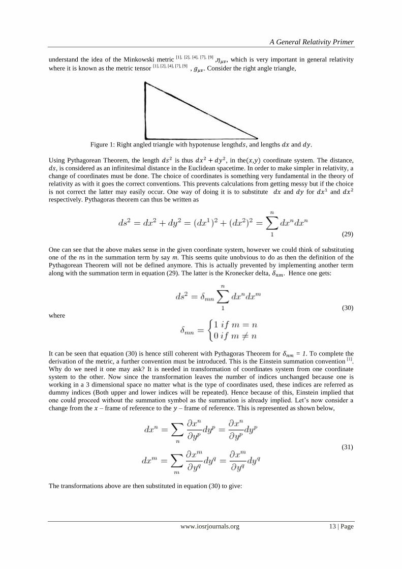
, . Consider the right angle triangle,

Figure 1: Right angled triangle with hypotenuse length , and lengths and .

Using Pythagorean Theorem, the length is thus , in the , coordinate system. The distance,

, is considered as an infinitesimal distance in the Euclidean spacetime. In order to make simpler in relativity, a

change of coordinates must be done. The choice of coordinates is something very fundamental in the theory of

relativity as with it goes the correct conventions. This prevents calculations from getting messy but if the choice

is not correct the latter may easily occur. One way of doing it is to substitute and for and

respectively. Pythagoras theorem can thus be written as

(29)

One can see that the above makes sense in the given coordinate system, however we could think of substituting

one of the ns in the summation term by say m. This seems quite unobvious to do as then the definition of the

Pythagorean Theorem will not be defined anymore. This is actually prevented by implementing another term

along with the summation term in equation (29). The latter is the Kronecker delta, . Hence one gets:

(30)

where

It can be seen that equation (30) is hence still coherent with Pythagoras Theorem for = 1. To complete the

derivation of the metric, a further convention must be introduced. This is the Einstein summation convention [1]

.

Why do we need it one may ask? It is needed in transformation of coordinates system from one coordinate

system to the other. Now since the transformation leaves the number of indices unchanged because one is

working in a 3 dimensional space no matter what is the type of coordinates used, these indices are referred as

dummy indices (Both upper and lower indices will be repeated). Hence because of this, Einstein implied that

one could proceed without the summation symbol as the summation is already implied. Let‟s now consider a

change from the – frame of reference to the – frame of reference. This is represented as shown below,

(31)

The transformations above are then substituted in equation (30) to give:



(32)

where ∑ ∑

, the latter is the metric tensor (or the Minkowski metric in special relativity)

which will be extensively used in the general theory of relativity. Equation (32) can thus be written as

, where = {

, hence recovering Pythagoras theorem in flat (Euclidean space)

when p = q. When p q, this implies that Pythagoras Theorem (Euclidean geometry) is no more valid in the

description of space. The term is thus a correction to this allowing the bridging between the theories of

special and general relativity. In the Minkowski spacetime, the interval between any two event A and B is thus

defined as [9]

(33)

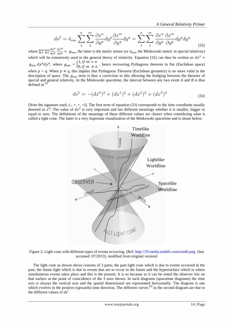
[Note the signature used, (-, +, +, +)]. The first term of equation (33) corresponds to the time coordinate usually

denoted as . The value of is very important and has different meanings whether it is smaller, bigger or

equal to zero. The definitions of the meanings of these different values are clearer when considering what is

called a light cone. The latter is a very important visualization of the Minkowski spacetime and is shone below:

Figure 2: Light cone with different types of events occurring. [Ref: http://29.media.tumblr.com/tumbl.png (last

accessed: 07/2013), modified from original version]

The light cone as shown above consists of 3 parts; the past light cone which is due to events occurred in the

past, the future light which is due to events that are to occur in the future and the hypersurface which is where

simultaneous events takes place and this is the present. It is so because as it can be noted the observer lies on

that surface at the point of coincidence of the 3 axes shown. In such diagrams (spacetime diagrams) the time

axis is always the vertical axis and the spatial dimensional are represented horizontally. The diagram is one

which evolves in the positive (upwards) time direction. The different curves [8]

in the second diagram are due to

the different values of ds2.

Timelike

Worldline

Lightlike

Worldline

Spacelike

Worldline

http://29.media.tumblr.com/tumblr_kz18bvVfBz1qb0ukuo1_400.png



What does the above mean? A spacelike interval as shone in the figure on the left (2b) is an event which cannot

be seen occurring at the same time at two distinct locations which are very far apart, it can be noticed that

spacelike event occurs on the hypersurface of the present at a unique time. A timelike interval is the difference

between events which occur at two or more different time but are related to each other. A lightlike interval is

when a ray of light travel between two events. The gradient of the cone‟s surface cannot be less than unity. A

particle undisturbed which goes through all the sets of past and future event is said to be following its world

line. These different types of intervals can be proved using the Lorentz transformation [2], [9]

which has not been

included in this paper.

IV. Tensor Analysis Tensors have been around in the mathematical world since the time of Gauss. They are extremely

important objects in both mathematics and physics. Tensors are the primary tools needed for the understanding

of the theory of relativity. The former also applies in special relativity as we have seen with the Minkowskian

metric. In classical electrodynamics, Maxwell equation and the continuity equation can be written in a more

compact and elegant way using tensor notation.

A tensor is a relationship between any 2 vectors. If the relationship implies that the tensor has a rank of 0 in one

frame of reference, this means that it will have that value in ALL frames of reference.

In the theory of special relativity, transformation law applies to vectors from one frame of reference to the other

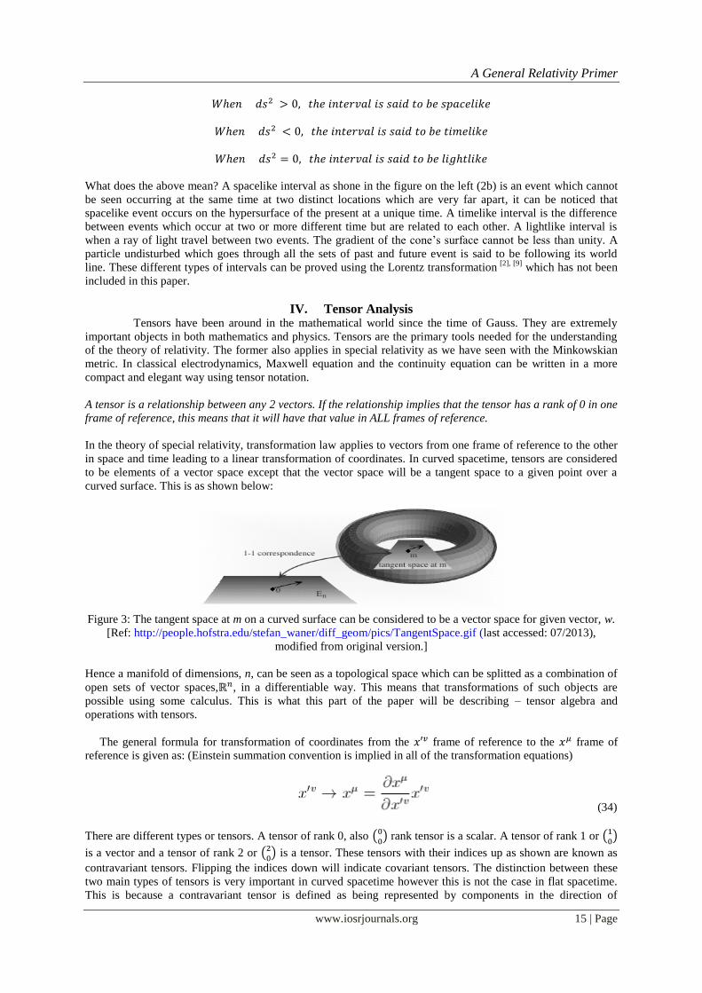
in space and time leading to a linear transformation of coordinates. In curved spacetime, tensors are considered

to be elements of a vector space except that the vector space will be a tangent space to a given point over a

curved surface. This is as shown below:

Figure 3: The tangent space at m on a curved surface can be considered to be a vector space for given vector, w.

[Ref: http://people.hofstra.edu/stefan_waner/diff_geom/pics/TangentSpace.gif (last accessed: 07/2013),

modified from original version.]

Hence a manifold of dimensions, n, can be seen as a topological space which can be splitted as a combination of

open sets of vector spaces, , in a differentiable way. This means that transformations of such objects are

possible using some calculus. This is what this part of the paper will be describing – tensor algebra and

operations with tensors.

The general formula for transformation of coordinates from the frame of reference to the frame of

reference is given as: (Einstein summation convention is implied in all of the transformation equations)

(34)

There are different types or tensors. A tensor of rank 0, also ( ) rank tensor is a scalar. A tensor of rank 1 or (

)

is a vector and a tensor of rank 2 or ( ) is a tensor. These tensors with their indices up as shown are known as

contravariant tensors. Flipping the indices down will indicate covariant tensors. The distinction between these

two main types of tensors is very important in curved spacetime however this is not the case in flat spacetime.

This is because a contravariant tensor is defined as being represented by components in the direction of

http://people.hofstra.edu/stefan_waner/diff_geom/pics/TangentSpace.gif



coordinate increase whereas a covariant tensor is defined as being represented by components in the direction

orthogonal to that of the coordinate constant surfaces. Hence in flat spacetime these two types of tensors are

made to coincide causing the distinction to vanish.

A. Contravariant and Covariant Tensors

Let be a contravariant tensor of rank 1 (contravariant vector). Transformation for a contravariant

tensor is:

(35)

Transformation for a covariant tensor is just the same thing except that some swapping of indices must be done:

(36)

The capital gamma symbol, Λ, is also used to indicate the differential leading to a transformation of coordinate.

The transformation of a second rank tensor is just an extension of the above. A second rank tensor is the result

of the outer product of two rank ( ) tensors.

Contravariant tensor of rank 2,

(37)

(38)

Covariant tensor of rank 2,

(39)

(40)

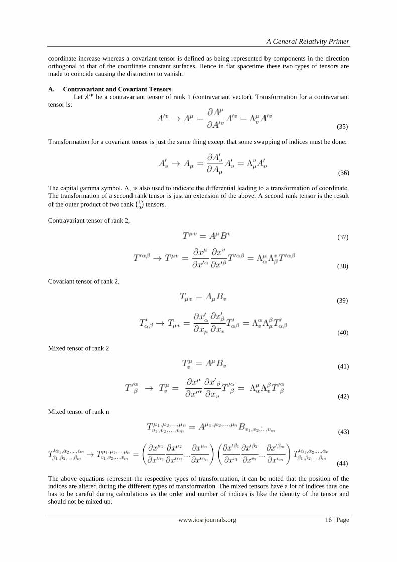
Mixed tensor of rank 2

(41)

(42)

Mixed tensor of rank n

(43)

(44)

The above equations represent the respective types of transformation, it can be noted that the position of the

indices are altered during the different types of transformation. The mixed tensors have a lot of indices thus one

has to be careful during calculations as the order and number of indices is like the identity of the tensor and

should not be mixed up.



B. Basic Operations with Tensors

Equality: Tensors are said to be equal if they have the same contravariant and covariant rank.

Associativity and Commutativity: Tensors of the same type can be added or subtracted with each other to

give a tensor of the same rank. Addition is thus associative and commutative.

Outer product: This is the product of two tensors whose rank is given as the sum of the ranks of the two

individual tensors.

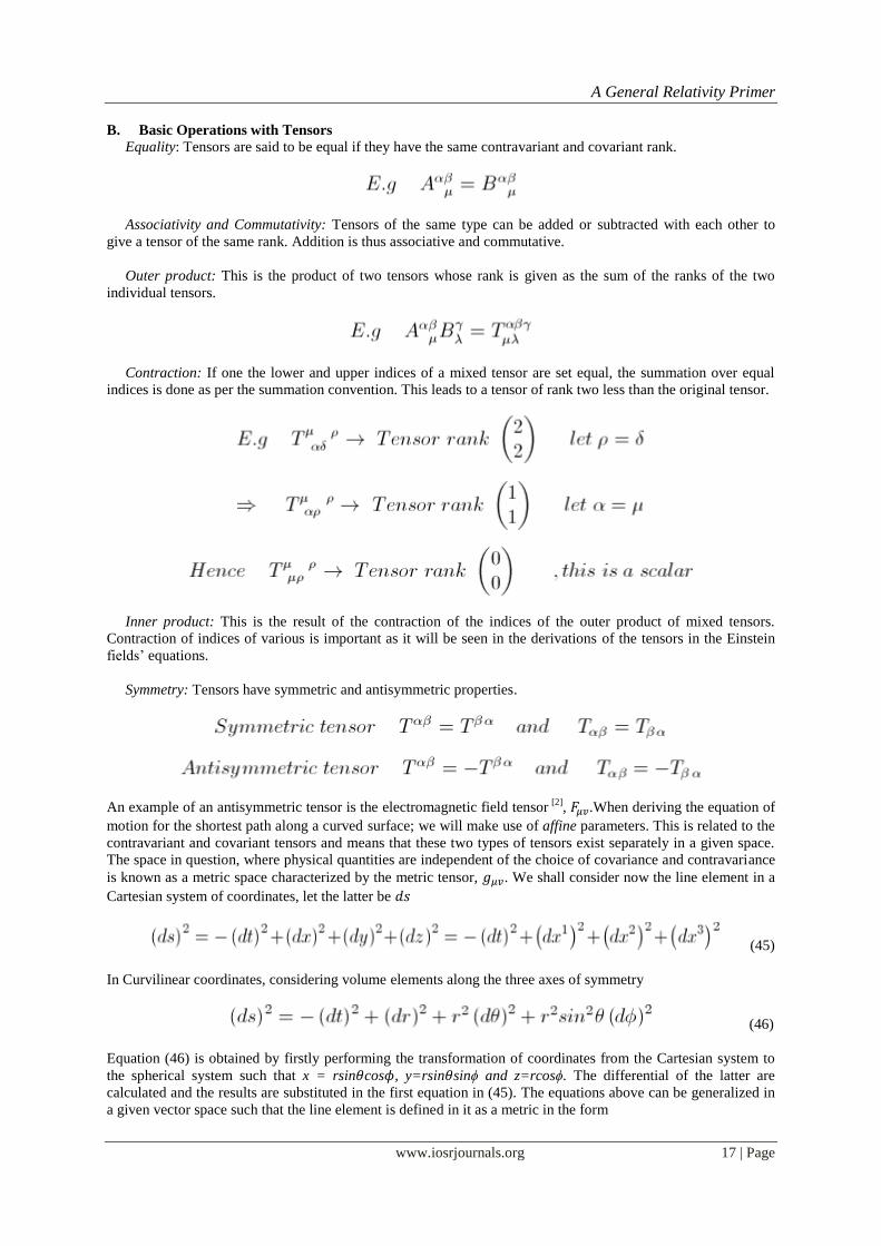
Contraction: If one the lower and upper indices of a mixed tensor are set equal, the summation over equal

indices is done as per the summation convention. This leads to a tensor of rank two less than the original tensor.

Inner product: This is the result of the contraction of the indices of the outer product of mixed tensors.

Contraction of indices of various is important as it will be seen in the derivations of the tensors in the Einstein

fields‟ equations.

Symmetry: Tensors have symmetric and antisymmetric properties.

An example of an antisymmetric tensor is the electromagnetic field tensor [2]

, .When deriving the equation of

motion for the shortest path along a curved surface; we will make use of affine parameters. This is related to the

contravariant and covariant tensors and means that these two types of tensors exist separately in a given space.

The space in question, where physical quantities are independent of the choice of covariance and contravariance

is known as a metric space characterized by the metric tensor, . We shall consider now the line element in a

Cartesian system of coordinates, let the latter be

(45)

In Curvilinear coordinates, considering volume elements along the three axes of symmetry

(46)

Equation (46) is obtained by firstly performing the transformation of coordinates from the Cartesian system to

the spherical system such that x = rsin cos , y=rsin sinϕ and z=rcosϕ. The differential of the latter are

calculated and the results are substituted in the first equation in (45). The equations above can be generalized in

a given vector space such that the line element is defined in it as a metric in the form



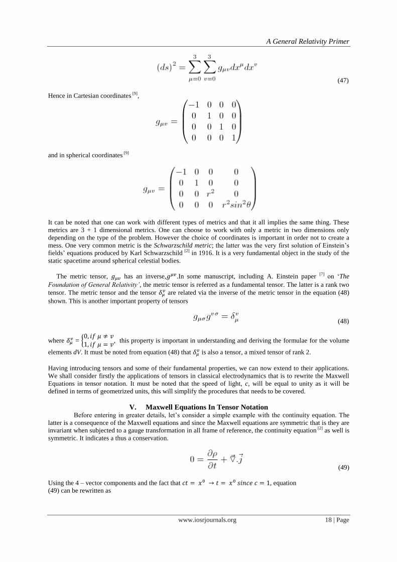
(47)

Hence in Cartesian coordinates [9]

,

and in spherical coordinates [9]

It can be noted that one can work with different types of metrics and that it all implies the same thing. These

metrics are 3 + 1 dimensional metrics. One can choose to work with only a metric in two dimensions only

depending on the type of the problem. However the choice of coordinates is important in order not to create a

mess. One very common metric is the Schwarzschild metric; the latter was the very first solution of Einstein‟s

fields‟ equations produced by Karl Schwarzschild [2]

in 1916. It is a very fundamental object in the study of the

static spacetime around spherical celestial bodies.

The metric tensor, has an inverse, .In some manuscript, including A. Einstein paper [7]

on „The

Foundation of General Relativity’, the metric tensor is referred as a fundamental tensor. The latter is a rank two

tensor. The metric tensor and the tensor are related via the inverse of the metric tensor in the equation (48)

shown. This is another important property of tensors

(48)

where = {

, this property is important in understanding and deriving the formulae for the volume

elements dV. It must be noted from equation (48) that is also a tensor, a mixed tensor of rank 2.

Having introducing tensors and some of their fundamental properties, we can now extend to their applications.

We shall consider firstly the applications of tensors in classical electrodynamics that is to rewrite the Maxwell

Equations in tensor notation. It must be noted that the speed of light, c, will be equal to unity as it will be

defined in terms of geometrized units, this will simplify the procedures that needs to be covered.

V. Maxwell Equations In Tensor Notation Before entering in greater details, let‟s consider a simple example with the continuity equation. The

latter is a consequence of the Maxwell equations and since the Maxwell equations are symmetric that is they are

invariant when subjected to a gauge transformation in all frame of reference, the continuity equation [2]

as well is

symmetric. It indicates a thus a conservation.

(49)

Using the 4 – vector components and the fact that , equation

(49) can be rewritten as



(50)

(51)

Equation above is hence the continuity equation in tensor notation and it is indeed a scalar (Lorentz invariant in

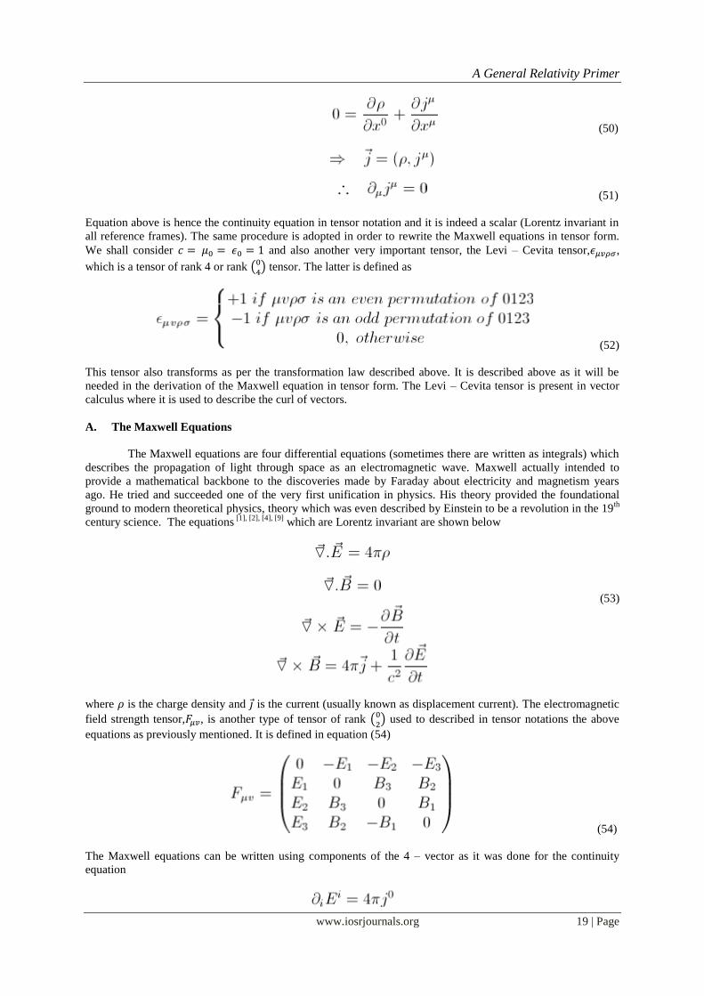
all reference frames). The same procedure is adopted in order to rewrite the Maxwell equations in tensor form.

We shall consider and also another very important tensor, the Levi – Cevita tensor, ,

which is a tensor of rank 4 or rank ( ) tensor. The latter is defined as

(52)

This tensor also transforms as per the transformation law described above. It is described above as it will be

needed in the derivation of the Maxwell equation in tensor form. The Levi – Cevita tensor is present in vector

calculus where it is used to describe the curl of vectors.

A. The Maxwell Equations

The Maxwell equations are four differential equations (sometimes there are written as integrals) which

describes the propagation of light through space as an electromagnetic wave. Maxwell actually intended to

provide a mathematical backbone to the discoveries made by Faraday about electricity and magnetism years

ago. He tried and succeeded one of the very first unification in physics. His theory provided the foundational

ground to modern theoretical physics, theory which was even described by Einstein to be a revolution in the 19th

century science. The equations [1], [2], [4], [9]

which are Lorentz invariant are shown below

(53)

where is the charge density and is the current (usually known as displacement current). The electromagnetic

field strength tensor, , is another type of tensor of rank ( ) used to described in tensor notations the above

equations as previously mentioned. It is defined in equation (54)

(54)

The Maxwell equations can be written using components of the 4 – vector as it was done for the continuity

equation



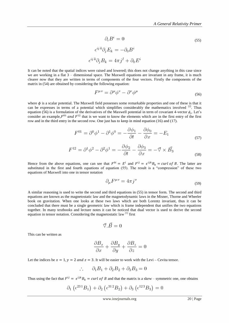
(55)

It can be noted that the spatial indices were raised and lowered; this does not change anything in this case since

we are working in a flat 3 – dimensional space. The Maxwell equations are invariant in any frame, it is much

clearer now that they are written in terms of components of the four vectors. Firstly the components of the

matrix in (54) are obtained by considering the following equation:

(56)

where is a scalar potential. The Maxwell field possesses some remarkable properties and one of these is that it

can be expresses in terms of a potential which simplifies considerably the mathematics involved [2]

. Thus

equation (56) is a formulation of the derivatives of the Maxwell potential in term of covariant 4-vector ϕμ. Let‟s

consider an example, that is we want to know the elements which are in the first entry of the first

row and in the third entry in the second row. One just has to keep in mind equation (16) and (17).

(57)

(58)

Hence from the above equations, one can see that and . The latter are

substituted in the first and fourth equations of equation (55). The result is a “compression” of these two

equations of Maxwell into one in tensor notation

(59)

A similar reasoning is used to write the second and third equations in (55) in tensor form. The second and third

equations are known as the magnetostatic law and the magnetodynamic laws in the Misner, Thorne and Wheeler

book on gravitation. When one looks at these two laws which are both Lorentz invariant, thus it can be

concluded that there must be a single geometric law which is frame independent that unifies the two equations

together. In many textbooks and lecture notes it can be noticed that dual vector is used to derive the second

equation in tensor notation. Considering the magnetostatic law [1]

first

This can be written as

Let the indices be . It will be easier to work with the Levi – Cevita tensor.

Thus using the fact that and that the matrix is a skew – symmetric one, one obtains



The exact same thing is done with the magnetodynamic law; the only difference is that one get a curl, by

keeping equation (56) in mind the appropriate component can be easily found. Also the choice indices may not

be only (1, 2, 3) as for the above proof. It can be for example (0, 2, and 3). One will then end up with something

like;

Thus it can be concluded that the final unifying equation in tensor notation of equation two and three in (55) can

be written as: [This is actually an exercise [1]

(Exercise 3.7 Pg. 81 in MTW – Gravitation)]

(60)

This last part is actually about covariant derivative, here we have applied in flat space but if we need to

generalize this to curve space, one just has to replace the which indicates covariant derivative. This is

how calculus is done on curved space; one cannot simply apply ordinary calculus. Actually this will be the next

part of the paper, I shall try to apply ordinary calculus and it will be noticed that a correction is actually needed

which will lead us to consider covariant derivatives.

VII. A Brief Introduction To The Riemannian Topology In this section, the mathematical tools and principle related to the curvature of spacetime will be

explored. In a flat space, the shortest distance between any two points is a straight line whose distance is easily

calculated using Euclidean geometry. However in a curved space, things are quite different, this can be noticed

by drawing a right angle triangle on a curved surface – say on a globe. The sum of the angles is bigger than

1800. Thus one can conclude that Euclidean geometry no more holds and that some kind of correction or

modification needs to be made. This is what general relativity does. One need then to understand how to figure

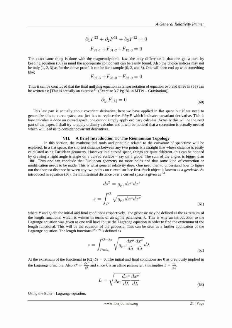
out the shortest distance between any two points on curved surface first. Such object is known as a geodesic. As

introduced in equation (30), the infinitesimal distance over a curved space is given as [6]

(61)

where P and Q are the initial and final conditions respectively. The geodesic may be defined as the extremum of

the length functional which is written in terms of an affine parameter, λ. This is why an introduction to the

Lagrange equation was given as one will have to use the Lagrange equation in order to find the extremum of the

length functional. This will be the equation of the geodesic. This can be seen as a further application of the

Lagrange equation. The length functional [6], [9]

is defined as

(62)

At the extremum of the functional in (62), . The initial and final conditions are 0 as previously implied in

the Lagrange principle. Also

and since λ is an affine parameter

, this implies

.

(63)

Using the Euler - Lagrange equation,



(64)

(65)

Now considering,

As per product rule,

Using chain rule,

(66)

Equation (65) and (66) are then substituted in the Euler – Lagrange equation (64),

Both sides of the equation can be divided by -1.Simplifying the terms reduces equation (66) to,

(67)

Equation (67) is thus known as the geodesic equation. This is the equation which describes the motion of a test

particle on an affine geodesic; it is a very fundamental equation as it will introduce us to something new – The

Christoffel symbol [1]

. The latter is very important in defining the various tensors related to curvature of the

Riemannian spacetime. The Christoffel symbol related to equation (67) is given as, . Hence equation (67)

can be written as,

(68)

where the Christoffel symbol in this case is defined as



where represents the Christoffel symbol of the first kind [4]

. Since equation (68) describes the motion of a

body on a curved surface, it is not surprising to see that it indeed contain the metric tensor. This is because the

latter characterizes the curvature of spacetime. A very good mathematics textbook [12]

, “Mathematical Methods

for Physics and Engineering by Riley, Hobson and Bence”, provides a deeper understanding of tensors for

undergraduates. There are two types of Christoffel symbols. The Christoffel symbol of the second kind is

obtained by multiplying equation (68) throughout by the inverse of the metric tensor,

(69)

(70)

The Christoffel symbol can also be derived using polar coordinates, for example one may consider the metric

, where

is a constant. The geodesic equation is derived using the Euler –

Lagrange equation. The kinetic Lagrangian is defined as;

(71)

( ) will read

(72)

(73)

and ( ) will read

(74)

(75)

One can now note that equation (73) and (75) are in a form similar to (69), we now have to identify the

Christoffel symbols for each case. One may ask why is the Lagrange method used?. This is because as it can be

noted, the metric has 8 different combination of , this means there are eight Christoffel symbols to be



found which is tedious. Thus with the above method only two of them is calculated and we automatically imply

that the others are 0 as per symmetry principle. Hence the Christoffel symbols [5]

for (73) and (75) are

respectively

(76)

The above calculation is actually a common exercise found in many relativity textbooks. For this reason I will

proceed a bit faster and introduce some new tensors which are directly linked to curvature of space. These will

be further discussed and derived in a later section of the paper. After having defined the Christoffel symbols,

one can now calculate the Riemann tensor for the above case; the latter is given as

(77)

(78)

(79)

Equation (79) is the inverse of (77), with the above one can also obtain the Ricci tensor which is obtained from a

contraction of the Riemann tensor. A further tensor which is the curvature scalar is obtained by contraction of

the Ricci tensor. This is shown below

(80)

(81)

Hence the above is a typical example of the type of calculations done in general relativity, the difficulty lies in

the manipulation of indices, one can note that the minus has been omitted, this is due to *symmetry principles.

In this calculation, the polar form of the metric tensor was used. One can do the same thing for other types of

metric such as the Schwarzschild metric. There are many types of metrics which leads to the improvement of

Einstein theory of general relativity by providing solutions to the Einstein‟s field equations – the simplest being

the Schwarzschild metric which is in accordance with Birkhoff‟s theorem [2]

.

Birkhoff’s Theorem implies the Schwarzschild solution is the most general solution in vacuum that describes the

space time in the exterior of a massive source, with spherical symmetry, even if the source is itself non

static.(For example; a Pulsar).

The next and final subject of this paper will be the fields‟ equations but before going deeper into the topic, I

will have to firstly define the covariant derivative which a fundamental tool for working on curved topologies.

The former will include the Christoffel symbols, it must be noted that the latter is a correction to be brought

when one deals with the mathematics of curved space. For example, considering equation (69), we know that

the affine parameters are related to an arc as per the correction. However on a flat space, the Christoffel symbols

all vanish and the equation is simply a homogenous second order differential which is easily solved giving

equation of a line. Hence the Christoffel symbols are very important in the following section.

A covariant derivative is defined as a normal derivative plus a correction term which is a Christoffel symbol.

The covariant derivative is derived by firstly considering transformation of tensors in different frames on a

curved space. We know that tensors are invariant in any frames of reference, thus when carrying out the

transformation this will not be the case unless one considers the compensation brought by the correction term.

Hence a covariant derivative [4]

is defined as



(82)

Note: The metric tensor, , is covariantly constant [4]

, this means that in all frames of reference.

The transformation of a vector on a curved surface is defined as [4]

(83)

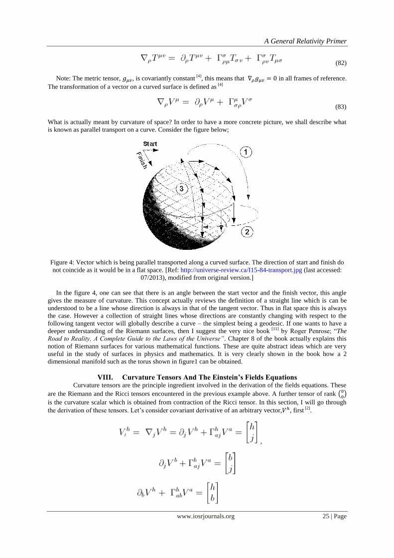
What is actually meant by curvature of space? In order to have a more concrete picture, we shall describe what

is known as parallel transport on a curve. Consider the figure below;

Figure 4: Vector which is being parallel transported along a curved surface. The direction of start and finish do

not coincide as it would be in a flat space. [Ref: http://universe-review.ca/I15-84-transport.jpg (last accessed:

07/2013), modified from original version.]

In the figure 4, one can see that there is an angle between the start vector and the finish vector, this angle

gives the measure of curvature. This concept actually reviews the definition of a straight line which is can be

understood to be a line whose direction is always in that of the tangent vector. Thus in flat space this is always

the case. However a collection of straight lines whose directions are constantly changing with respect to the

following tangent vector will globally describe a curve – the simplest being a geodesic. If one wants to have a

deeper understanding of the Riemann surfaces, then I suggest the very nice book [11]

by Roger Penrose; “The

Road to Reality, A Complete Guide to the Laws of the Universe”. Chapter 8 of the book actually explains this

notion of Riemann surfaces for various mathematical functions. These are quite abstract ideas which are very

useful in the study of surfaces in physics and mathematics. It is very clearly shown in the book how a 2

dimensional manifold such as the torus shown in figure1 can be obtained.

VIII. Curvature Tensors And The Einstein’s Fields Equations Curvature tensors are the principle ingredient involved in the derivation of the fields equations. These

are the Riemann and the Ricci tensors encountered in the previous example above. A further tensor of rank ( )

is the curvature scalar which is obtained from contraction of the Ricci tensor. In this section, I will go through

the derivation of these tensors. Let‟s consider covariant derivative of an arbitrary vector, , first [2]

.

,

http://universe-review.ca/I15-84-transport.jpg



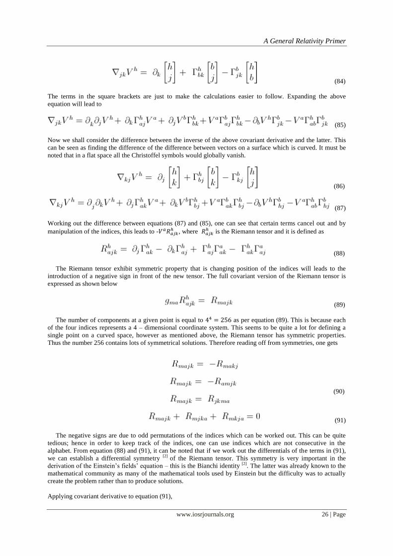
(84)

The terms in the square brackets are just to make the calculations easier to follow. Expanding the above

equation will lead to

(85)

Now we shall consider the difference between the inverse of the above covariant derivative and the latter. This

can be seen as finding the difference of the difference between vectors on a surface which is curved. It must be

noted that in a flat space all the Christoffel symbols would globally vanish.

(86)

(87)

Working out the difference between equations (87) and (85), one can see that certain terms cancel out and by

manipulation of the indices, this leads to - , where

is the Riemann tensor and it is defined as

(88)

The Riemann tensor exhibit symmetric property that is changing position of the indices will leads to the

introduction of a negative sign in front of the new tensor. The full covariant version of the Riemann tensor is

expressed as shown below

(89)

The number of components at a given point is equal to as per equation (89). This is because each

of the four indices represents a 4 – dimensional coordinate system. This seems to be quite a lot for defining a

single point on a curved space, however as mentioned above, the Riemann tensor has symmetric properties.

Thus the number 256 contains lots of symmetrical solutions. Therefore reading off from symmetries, one gets

(90)

(91)

The negative signs are due to odd permutations of the indices which can be worked out. This can be quite

tedious; hence in order to keep track of the indices, one can use indices which are not consecutive in the

alphabet. From equation (88) and (91), it can be noted that if we work out the differentials of the terms in (91),

we can establish a differential symmetry [2]

of the Riemann tensor. This symmetry is very important in the

derivation of the Einstein‟s fields‟ equation – this is the Bianchi identity [2]

. The latter was already known to the

mathematical community as many of the mathematical tools used by Einstein but the difficulty was to actually

create the problem rather than to produce solutions.

Applying covariant derivative to equation (91),



(92)

(93)

Contracting the indices of the Riemann tensor leads to the formation of a tensor of rank 2 which is the Ricci

tensor [2]

, .

(94)

Contracting the above one more time leads to a tensor of rank 0. This is the curvature scalar.

(95)

The Principle of Equivalence states that there is no difference between the effects encountered by a body

falling in a uniformly accelerating frame of reference and a body situated in a non – accelerating frame of

reference in a uniform gravitational field [2],[9]

.

Having defined the fundamentals aspects of the theory of general relativity, we can now proceed to the

explanation and derivation of the fields‟ equation. There are 16 of the Einstein‟s fields‟ equations. This is

because the general equation is written in terms of rank ( ) tensors such that each index contains 4 components

(more precisely 3 + 1 components) hence total number [2]

of components hence total number of equations will

be 42 = 16. However due to symmetry of 6 tensors in the equations one is left with only 10 of the fields‟

equation. These equations are non – linear partial differential equations and are actually quite difficult to solve

without the assumption of symmetry of the equations in a given coordinate system. There are different ways of

deriving the Einstein‟s fields‟ equation; For example one can use the twice contracted Bianchi identity in order

to obtain the Einstein tensor and hence work out the general equation or one can make use of a more physical

way using the Einstein – Hilbert action, from the variational principle, the general equation is obtained by

considering the extremum of the functional. This will however be done in a slightly simpler way by firstly

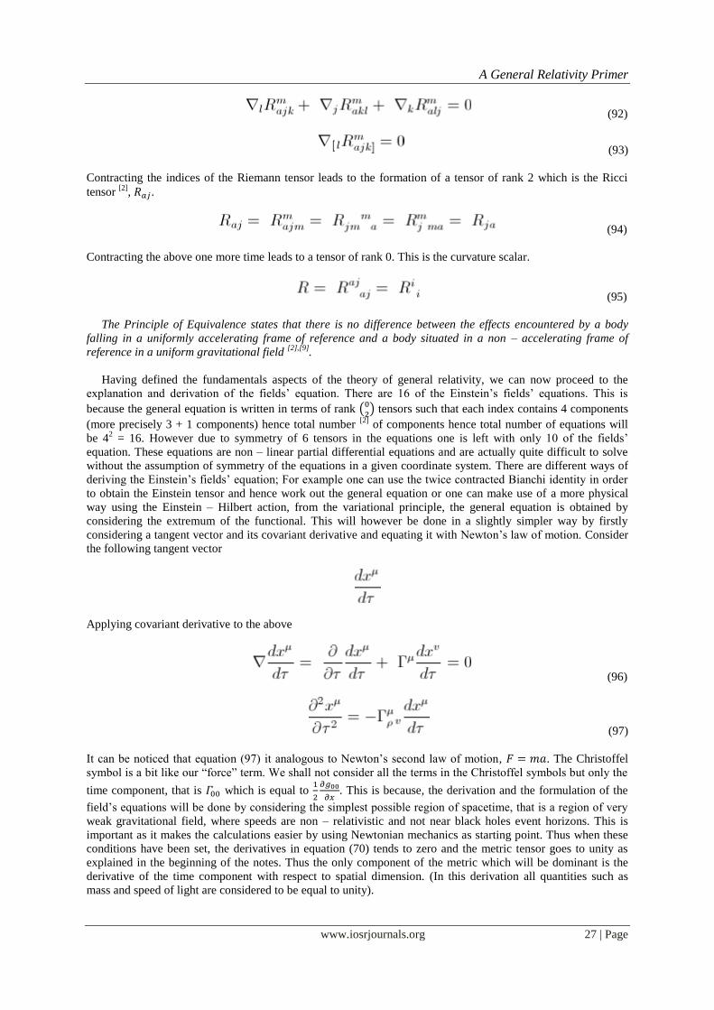
considering a tangent vector and its covariant derivative and equating it with Newton‟s law of motion. Consider

the following tangent vector

Applying covariant derivative to the above

(96)

(97)

It can be noticed that equation (97) it analogous to Newton‟s second law of motion, . The Christoffel

symbol is a bit like our “force” term. We shall not consider all the terms in the Christoffel symbols but only the

time component, that is which is equal to

. This is because, the derivation and the formulation of the

field‟s equations will be done by considering the simplest possible region of spacetime, that is a region of very

weak gravitational field, where speeds are non – relativistic and not near black holes event horizons. This is

important as it makes the calculations easier by using Newtonian mechanics as starting point. Thus when these

conditions have been set, the derivatives in equation (70) tends to zero and the metric tensor goes to unity as

explained in the beginning of the notes. Thus the only component of the metric which will be dominant is the

derivative of the time component with respect to spatial dimension. (In this derivation all quantities such as

mass and speed of light are considered to be equal to unity).



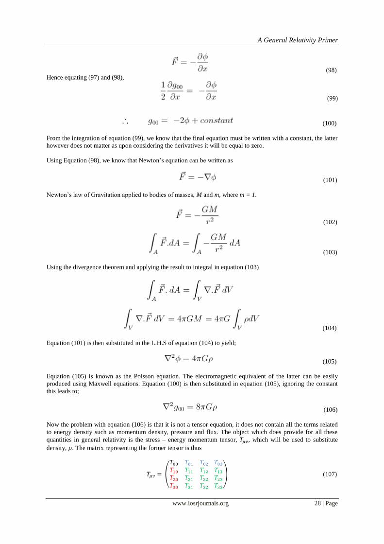
(98)

Hence equating (97) and (98),

(99)

(100)

From the integration of equation (99), we know that the final equation must be written with a constant, the latter

however does not matter as upon considering the derivatives it will be equal to zero.

Using Equation (98), we know that Newton‟s equation can be written as

(101)

Newton‟s law of Gravitation applied to bodies of masses, M and m, where m = 1.

(102)

(103)

Using the divergence theorem and applying the result to integral in equation (103)

(104)

Equation (101) is then substituted in the L.H.S of equation (104) to yield;

(105)

Equation (105) is known as the Poisson equation. The electromagnetic equivalent of the latter can be easily

produced using Maxwell equations. Equation (100) is then substituted in equation (105), ignoring the constant

this leads to;

(106)

Now the problem with equation (106) is that it is not a tensor equation, it does not contain all the terms related

to energy density such as momentum density, pressure and flux. The object which does provide for all these

quantities in general relativity is the stress – energy momentum tensor, , which will be used to substitute

density, . The matrix representing the former tensor is thus

(

) (107)



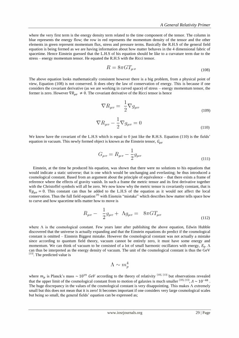
where the very first term is the energy density term related to the time component of the tensor. The column in

blue represents the energy flow; the row in red represents the momentum density of the tensor and the other

elements in green represent momentum flux, stress and pressure terms. Basically the R.H.S of the general field

equation is being formed as we are having information about how matter behaves in the 4 dimensional fabric of

spacetime. Hence Einstein guessed that the L.H.S of his equation should be like to a curvature term due to the

stress – energy momentum tensor. He equated the R.H.S with the Ricci tensor.

(108)

The above equation looks mathematically consistent however there is a big problem, from a physical point of

view, Equation (108) is not conserved. It does obey the law of conservation of energy. This is because if one

considers the covariant derivative (as we are working in curved space) of stress – energy momentum tensor, the

former is zero. However . The covariant derivative of the Ricci tensor is hence

(109)

(110)

We know have the covariant of the L.H.S which is equal to 0 just like the R.H.S. Equation (110) is the fields‟

equation in vacuum. This newly formed object is known as the Einstein tensor,

(111)

Einstein, at the time he produced his equation, was shown that there were no solutions to his equations that

would indicate a static universe; that is one which would be unchanging and everlasting; he thus introduced a

cosmological constant. Based from an argument about the principle of equivalence – that there exists a frame of

reference where the effects of gravity vanish. In such a frame the metric tensor and its first derivative together

with the Christoffel symbols will all be zero. We now know why the metric tensor is covariantly constant, that is

. This constant can thus be added to the L.H.S of the equation as it would not affect the local

conservation. Thus the full field equation [9]

with Einstein “mistake” which describes how matter tells space how

to curve and how spacetime tells matter how to move is

(112)

where Λ is the cosmological constant. Few years later after publishing the above equation, Edwin Hubble

discovered that the universe is actually expanding and that the Einstein equations do predict if the cosmological

constant is omitted – Einstein Biggest mistake. However the cosmological constant was not actually a mistake

since according to quantum field theory, vacuum cannot be entirely zero, it must have some energy and

momentum. We can think of vacuum to be consisted of a lot of small harmonic oscillators with energy, Λ

can thus be interpreted as the energy density of vacuum. The unit of the cosmological constant is thus the GeV [13]

. The predicted value is

where is Planck‟s mass according to the theory of relativity [10], [13]

but observations revealed

that the upper limit of the cosmological constant from to motion of galaxies is much smaller [10], [13]

, .

The huge discrepancy in the values of the cosmological constant is very disappointing. This makes Λ extremely

small but this does not mean that it is zero! It becomes important if one considers very large cosmological scales

but being so small, the general fields‟ equation can be expressed as;



(113)

The Einstein‟s field‟s equations are now obtained; the above derivation is a very simple and informal one.

The equations of Einstein are actually 10 (as explained why above) nonlinear partial differential equations. This

makes it very difficult to find solutions of such equation even when considering the situation in vacuum; that is

when . The Einstein field‟s equations describe the fundamental interaction between curved spacetime

and matter – energy content leading to the curved spacetime. This interaction is obviously gravity. The

equations thus determine the geometry of spacetime as a result of the presence of mass – energy and linear

momentum. That is the solutions of the former equations are metric which are related to the stress – energy

momentum tensor. I will discuss one very simple solution of these equations a bit latter. However before I

consider a slightly more rigorous way of obtaining equation (113), then the Einstein – Hilbert action is the

correct starting point.

This is an action which is written in terms of the curvature scalar and the Lagrangian density for matter fields.

I shall use the Palatini Formalism that is to treat the metric and the connections (Christoffel symbols) as

independent degrees of freedom and vary each of these with respect to them.

(114)

Considering variation of the action,

(115)

We eventually assume that at the boundary, we can define the following

(116)

The stress – energy momentum tensor is related to the Lagrangian of matter fields as

(117)

(118)

Hence rearranging equation (118), one gets back to the Einstein‟s field‟s equation which is equation (113). The

above proof has been overly simplified to make things clearer. The Einstein – Hilbert action is a very elegant

way of representing the results of this very fundamental part of theoretical physics. This is why a very simple

description of the former was introduced briefly.

IX. The Schwarzschild Metric Having now explained the Einstein fields‟ equation, I shall give the very first solution of the latter

which was produced by Karl Schwarzschild [1], [2]

in 1916, few months after Einstein published his paper. This

first solution will be the Schwarzschild metric. Let‟s firstly consider the Lorentz transformation [9}

for time and

distance in a local frame of reference relative to the initial frame of reference in a static spherically symmetric

gravitational field. These are given as;

(119)



where is defined as the proper length, this is the time measured by a clock in rest frame of reference, is the

local spatial coordinate and is the velocity that the accelerated frame of reference must have in the absence of

a gravitational in order to have the same value in the stationary frame at a given coordinate . The metric for the

line element of that spacetime is the one used in equation (46), this is

(120)

Equation (119) is then substituted in the above metric and the velocity is substituted by the escape velocity

given as per the Newton‟s equation of classical mechanics which is

, where M is the mass of the

source of the gravitational field. The resulting metric is hence

(121)

This is the famous Schwarzschild metric [1], [2]

. The latter is used to obtain information about exterior

spacetime of spherically symmetric objects such as black holes and pulsating stars (pulsars). The above

derivation, as one can note, is very simple since it does not include calculations with tensors, this is the Lenz –

Shiff derivation. The actual derivation can be found in the paper ref. [8] which is a step – by – step derivation of

each of components of the Riemann tensor, the Ricci tensor and the curvature scalar. Being a rather lengthy

calculation, I preferred not include it in this review in order to keep it simple. It will be noted in many textbooks

that the (+, -, -, -) signature is used with the metric which is not the case in the above derivation.

References [1] Misner. C.W, Thorne. S. K, & Wheeler. J. A: GRAVITATION, W. H Freeman & Co., 1973.

[2] Rindler. W: Relativity, Special, General and Cosmological, Oxford University Press Inc., New York, 2006.

[3] Hawking. S: On the Shoulders of Giants, The Great Works of Physics and Astronomy, Penguin Books, Great Britain, 2003, Pg. 1214 – 1216.

[4] Schultz. B: A First Course in General Relativity, Cambridge University Press, New York, United States of America, 2009.

[5] Larsen. S: “Lots of Calculation in General Relativity”, 2013. [6] Chow. L.T: Mathematical Methods for Physicists: A Concise Introduction, Cambridge University Press, Australia, 2000.

[7] Einstein. A: “The Foundation of General Theory of Relativity”, In: The Collected Papers of Albert Einstein, Volume 6, The Berlin

Years, Writings 1914 – 1917. Edited by Kox. J.A, Klein. J. M and Schulmann. R, Princeton University Press, 1997.

[8] Simpson. D: “A Mathematical Derivation of the General Relativistic Schwarzschild Metric”, B.Sc. Thesis, East Tennessee State

University, 2007.

[9] Carroll, M. S: “Lecture Notes on General Relativity”, 1997, arXiv: gr – qc [9719019]. [10] Poudel. P.C, Khanal, U: “Estimation of the mass, cosmological constant and Kerr parameter of different galaxies using geodesic

motion in Kerr – de Sitter spacetime”, Scientific World, Vol. 10, No. 10, July 2012.

[11] Penrose. R: The Road to Reality, A Complete Guide to the Laws of the Universe, Vintage, London, 2005. [12] K. F. Riley, M. P. Hobson, S. J. Bence: Mathematical Methods for Physics and Engineering, third edition, Cambridge University

Press, 2006

[13] Luo. M. J: “The Cosmological Problem and the Re-interpretation of Time” arXiv: [1312.2759]. gen – ph, 10 Dec 2013.

a general relativity primer - iosr...

Documents