a general purpose configurable controller for indoors and outdoors gps-denied navigation for...
TRANSCRIPT

J Intell Robot SystDOI 10.1007/s10846-013-9953-0
A General Purpose Configurable Controller for Indoorsand Outdoors GPS-Denied Navigation for MultirotorUnmanned Aerial Vehicles
Jesús Pestana · Ignacio Mellado-Bataller ·Jose Luis Sanchez-Lopez · Changhong Fu ·Iván F. Mondragón · Pascual Campoy
Received: 1 September 2013 / Accepted: 13 September 2013© Springer Science+Business Media Dordrecht 2013
Abstract This research on odometry based GPS-denied navigation on multirotor Unmanned Aer-ial Vehicles is focused among the interactionsbetween the odometry sensors and the naviga-tion controller. More precisely, we present a con-troller architecture that allows to specify a speedspecified flight envelope where the quality ofthe odometry measurements is guaranteed. Thecontroller utilizes a simple point mass kinematicmodel, described by a set of configurable para-meters, to generate a complying speed plan. Forexperimental testing, we have used down-facingcamera optical-flow as odometry measurement.This work is a continuation of prior research tooutdoors environments using an AR Drone 2.0 ve-hicle, as it provides reliable optical flow on a wide
J. Pestana (B) · I. Mellado-Bataller ·J. L. Sanchez-Lopez · C. Fu · P. CampoyCentro de Automática y Robótica,CSIC-UPM, Madrid, Spaine-mail: [email protected]: http://www.vision4uav.com
P. Campoye-mail: [email protected]
I. F. MondragónCentro Tecnológico de Automatización Industrial,Pontificia Universidad Javeriana, Carrera 7 No 40-69,110311, Bogotá DC, Colombiae-mail: [email protected]: http://www.javeriana.edu.co/blogs/imondragon
range of flying conditions and floor textures. Ourexperiments show that the architecture is realiablefor outdoors flight on altitudes lower than 9 m. Aprior version of our code was utilized to competein the International Micro Air Vehicle Confer-ence and Flight Competition IMAV 2012. Thecode will be released as an open-source ROS stackhosted on GitHub.
Keywords Aerial robotics · Autonomousnavigation · Computer vision · Controlarchitectures and programming · Controlof UAVs · Micro aerial vehicles · Multirotormodeling and state estimation · Robotics ·Unmanned aerial vehicles
1 Introduction
The motivation of this work is to study the uti-lization of odometry measurements as a meansto stabilize the multirotor vehicle and to en-able GPS-denied autonomous navigation on in-doors and outdoors environments. An importantdifference between Vertical Take-Off and Land-ing (VTOL) vehicles, such as multirotors, andground robots is that they require to be stabi-lized using odometry or position measurements.If these measurements have a degraded qualityfor a long period of time (5–30 s), there is a highrisk of crashing due to small offset errors on the

J Intell Robot Syst
Inertial Measurement Unit (IMU) estimations.For experimental testing, we have used down-facing camera optical-flow as odometry measure-ment which is available and implemented on acommercial multirotor, the AR Drone 2.0, as ex-plained in [1]. This work is a continuation of priorresearch [2, 3] to experimental testing on outdoorsenvironments using an AR Drone 2.0 vehicle, asit provides reliable optical flow on a wide rangeof flying conditions and floor textures. Optical-flow based navigation strategies are an on-goingresearch topic on other robotics laboratories, forinstance: to enable fast calculations of the optical-flow [4], for collision and obstacle avoidance [5–7],and also to enable autonomous navigation [4, 8].
The presented research is focused on multiro-tor platforms, that are capable of flying in clut-tered areas and hover if controlled properly. Inorder to obtain a semi-autonomous flying plat-form that can be commanded with high-level com-mands by an operator, the state estimation andthe control problem must be addressed. On thepresented and recent work by our group [2, 3]a controller architecture to achieve stabilizationand navigation objectives has been designed andexperimentally tested on various multirotor ve-hicles: the AR Drone, the AR Drone 2, theAsctec Pelican and the LinkQuad quadrotors.Among other related work, the presented archi-tecture was implemented to compete, see Fig. 1,
Fig. 1 The Asctec Pelican quadrotor, equipped as ex-plained in Section 3, is shown flying in autonomous modeon the IMAV 2012 competition with an implementation ofthe controller presented in this paper. An EKF performsstate estimation on the odometry measurements, and itsestimation is fused with the position estimations from aMontecarlo Localization algorithm that is processing theLaser Range Finder readings. The quadrotor also had to be
able to fly safely on areas where no obstacles were in rangeof the laser sensor. In this image sequence the quadrotorpasses through a pair of poles using the laser sensor toestimate its position with respect to the poles. This flightgained the two IMAV 2012 awards stated in the intro-duction, see http://vision4uav.com/?q=IMAV12. The fullvideo of the flight is available online on http://vision4uav.com/?q=node/323
J Intell Robot Syst
in the International Micro Air Vehicle Confer-ence and Flight Competition IMAV 2012, gainingtwo awards: the Special Award on “Best Auto-matic Performance—IMAV 2012” and the secondoverall prize in the category of “Indoor FlightDynamics—Rotary Wing MAV”. The code re-lated to the presented work, which has been devel-oped in our research group, will be made availablein the near future as an open-source ROS Stackon GitHub [9–11], refer to Section 3.2 for moreinformation.
2 Related Work
The following cited work has shown that the navi-gation control loops must be designed taking intoaccount the non-linear dynamics of the multiro-tor, so that the control actions are approximatelydecoupled. If the control laws are well designedthe multirotor can perform smooth trajectoriesin position coordinates, while orientating its yawheading in any required direction.
Several labs have used a sub-millimeter accu-rate Vicon motion tracking system [12] to separatethe control and the state estimation problems.Researchers at the GRASP lab of the Universityof Pennsylvania, and at the ETH—IDSC—FlyingMachine Arena in the ETHZ, have been able toexecute precise trajectory following [13, 14], toperform aggresive maneuvers [14, 15], and to per-form collaborative tasks that require synchroniza-tion among the flying vehicles [16, 17]. Relying onVicon motion capture systems has simplified theresearch problem, which has shown that state es-timation is the key to enabling many autonomousapplications.
On the other hand, there are research groupsthat have shown successful autonomous multiro-tor navigation capabilities using only GPS posi-tioning data. The STARMAC project [18], fromStanford University has shown several experi-mental tests on outdoors ranging from trajectorytracking tasks [19] to performing flips and stall-turn maneuvers [20, 21].
Other groups have increased the situationalawareness of the mUAVs using optical flowsensors and cooperative robots. For instance, aground vehicle can estimate the position and
attitude of the mUAV [22]. These two researchworks [5, 7] are focused on navigation in corridorsand obstacle collision avoidance strategies usingmultiple optical flow sensors. In outdoors naviga-tion, optical flow sensors were used in a fixed-wingmUAV in [6] to avoid the collision with trees andother obstacles in a GPS waypoint trajectory.
3 System Overview
The presented research is a continuation on pre-vious work by the same authors [2, 3], that wasimplemented to participate on the IMAV 2012indoors dynamics challenge [23]. Images from theflight that gained the awards of the IMAV 2012competition are shown in Fig. 1, where the As-ctec Pelican was controlled by the software archi-tecture presented in this paper. In this case thelocalization problem was engaged using an Ex-tended Kalman Filter (EKF) to fuse the odometrymeasurements, and a Particle Filter (PF) with aknown map of the environment. The PF processedthe Laser Range Finder readings providing es-timated positions with respect to the pylons ofthe challenge [23]. The quadrotor also had to beable to fly safely on areas where no obstacleswere in range of the laser sensor, where only theEKF provides the necessary feedback to the con-troller. The focus of this paper is to further researhon safe navigation based on unperfect odome-try measurements, such as on-board optical flowmeasurements, and no position measurements areavailable.
This paper presents a navigation system archi-tecture which controller can be configured de-pending on the limitations that are imposed bythe kinematic capabilities of the vehicle, by themeasurement range of the speed estimators, or byprecision requirements of the task at hand. Theresult is an architecture that was experimentallytested on GPS-denied environments, and that canbe configured depending on the requirementsof each phase of a task. This allows to have asetup for fast trajectory following, and anotherto soften the control laws and make the vehi-cle navigate more precisely and slowly whenevernecessary.

J Intell Robot Syst
3.1 Hardware Architecture
The implemented hardware architecture is in-spired on the AR Drone quadrotor, which capa-bilities are described in [1]. An Asctec Pelicanquadrotor was equipped with a camera and anon-board computer to obtain a similar setup. Theadvantages of using the Asctec Pelican are that allthe algorithms can run on the on-board computer,and that the vehicle can be equipped with moresensors such as cameras and Laser Range Finders.
The Asctec Pelican shown in Fig. 2 is equippedwith an autopilot board that stabilizes the vehi-cle using information from GPS (only when out-doors), IMU, pressure altimeter and magnetome-ter fused using a Kalman Filter. This controlleris embedded, closed, unmodifiable but gains aretunable. This quadrotor has also been equippedwith a series of complementary sensors: a HokuyoScanning Laser Range Finder for horizontal depthmapping, a sonar altitude sensor for height estima-tion improvement and two cameras, one of them adownward looking sensor for velocity estimationbased on optical flow. The optical flow is calcu-lated using the OpenCV implementation of thepyramidal Lucas-Kanade algorithm for some im-age features selected by the Shi-Tomasi method.The state estimation and control processing areexeuted onboard in an Atom Board, which has a
dual core Atom 1.6 GHz processor with 1 GB ofRAM.
3.2 Software Architecture
The AR Drone and the Asctec Pelican wereboth accomodated to be compatible with theCVG Framework for interfacing with MAVs. Thisframework, also called “MAVwork”, was devel-oped by our research group; it is an open-sourceproject hosted on GitHub that can be accessedin [9], and its technical details can be found on[24, 25]. One of the advantages of the frameworkis that it offers a common type of interface forevery multirotor, allowing other software mod-ules, such as the controller, to be compatible withmultiple multirotors. The MAVwork interface hasbeen designed to be similar to the one offered bythe AR Drone, as this quadrotor has proven to beeasy and reliable to setup for experimental tests.Among other advantages, MAVwork offers na-tive take-off, landing and hovering flying modes;along with altitude hold capability. Figure 2 sum-marizes the interface functions that the API anddrone object offer to the developer.
As explained before, the experimental testsshown on this paper have been performed usingan AR Drone 2.0, as we are testing our soft-ware on outdoors environments. The advantage
Fig. 2 Pelican on CVGFramework forinterfacing with MAVs[9], user point of view.The Pelican offers severalfeedback channels: thetelemetry package withIMU attitude, horizontalbody speed and altitudedata, and camerafeedback channels whereeach camera is identifiedwith an ID value. Thedrone modes arereplicated from thoseavailable on the ARDrone

J Intell Robot Syst
of MAVwork is the experiments allows us tocontinue improving the framework for the othermultirotors as well. We perform software testingon the AR Drone 2 for multiple reasons: it is prac-tically harmless to people and third-party objects,the high quality of its speed estiamtion, its easeof use thanks to its built-in flying modes, its lowprice, and its robustness to chrases.
The different components of the control andstate estimation modules are shown in Fig. 3. AnExtended Kalman Filter is used as data fusionalgorithm to estimate the position and speed ofthe quadrotor. These estimates are then fed tothe high-level (HL) controller that obtains theposition, speed and feedforward commands thatare given to the mid-level controller. The plan-ning process that takes place in the HL controlleruses a simple kinematic model of the multirotorthat is specified by a set of configurable para-meters. The mid-level (ML) controller calculatesand sends the commands to MAVwork, whichacts as interface between the controller and thequadrotor. The HL and ML controllers are fur-ther described in Section 4. The state estima-tion and controller algorithms are available onan open-source project called “Multirotor Con-troller for MAVwork” hosted on GitHub thatcan be accessed in [10]. Its technical details areexplained in the Msc. Thesis [2] and on the presentpaper.
The multirotor is stabilized using odometry-based position estimates and for that reason theboundaries where the quality of these estimatesis lost must be determined. For instance, theoptical flow algorithm that is calculated on thedown-facing images is affected by the texture andreflectiveness of the floor surface, and also by thelighting conditions of the environment. The size ofthe floor texture details and the computing powerof the on-board computer set a maximum speedboundary on the speed estimation.
For instance, with the Pelican which tests canbe found on [2, 3], the maximum speed that couldbe reliably measured in the indoors playgroundwhere most of the tests where carried out wasabout 0.5–0.75 m/s, and so, this boundary was usedin our indoors tests. Based on our experience,the AR Drone 2 provides speed estimation feed-back even navigating at high speeds, up to 3 m/s.The direction of the speed estimation maintainsa good accuracy at all working conditions if theyaw rotations are kept low. On the other hand,the absolute value of the speed can be affected byseveral conditions. For example, when the droneswitches from ultrasound sensor based altitudeestimation to using the pressure sensor only, thespeed estimation is degraded. Also the speed mea-surement at speed in the 2–3 m/s speed range isnot accurate, but its enough to keep our controllerarchitecture working.
Fig. 3 General software architecture of the navigationcontroller. The State Estimation is used by the High-Levelcontroller to determine optimized reachable speed com-
mands to the mid-level controller, which sends commandsto the drone through the CVG Framework [9, 24, 25]
J Intell Robot Syst
The presented software architecture has beenimplemented on the AR Drone and Astec Pelicanquadrotors, and will be applied in the future toother multirotor platforms, more specifically toa LinkQuad [26] quadrotor and an OktoKopterfrom Mikrokopter [27]. The usage of a com-mon software architecture increases code qual-ity shareability and enables for different researchlines to work in a cohesive way towards the objec-tives of our group.
4 Navigation Controller
This section introduces the navigation controllerthat uses a set of configurable parameters to adaptto different multirotors and sensor limitations.The parameters are inspired by the STARMACproject work described in [19]. First a simple mul-tirotor point mass kinematic model is described.Then the high level controller state-machine is in-troduced with the description of the configurableparameters that are derived from the model. Thefinal part of the section introduces the middle-level controller.
4.1 Multirotor Point Mass Kinematic Model
A multirotor is a flying vehicle that can exert forcein any direction and thus can be simplified as apoint mass moving in the 3D space. The vehicletilts to exert force in the horizontal plane, andchanges the average propeller speeds to controlthe force in the altitude coordinate. A maximumspeed is also set by various reasons, for instance,due to the aerodynamic friction of the movementthrough the air. It is also important to take intoaccount that the multirotor is commanded usingfeedback loop control laws that produce a re-sponse that can be characterized by a little set ofparameters. The speed planifier can take advan-tage of a simple kinematic model built upon thesefacts in order to take decisions.
The body frame, {Xm, Ym, Zm}, of the vehi-cle, shown in Fig. 4, is described as follows. The{Xm, Ym} axis are horizontal and the Zm axispoints down to the floor. The Xm axis points to thefront of the vehicle and the Ym axis points to the
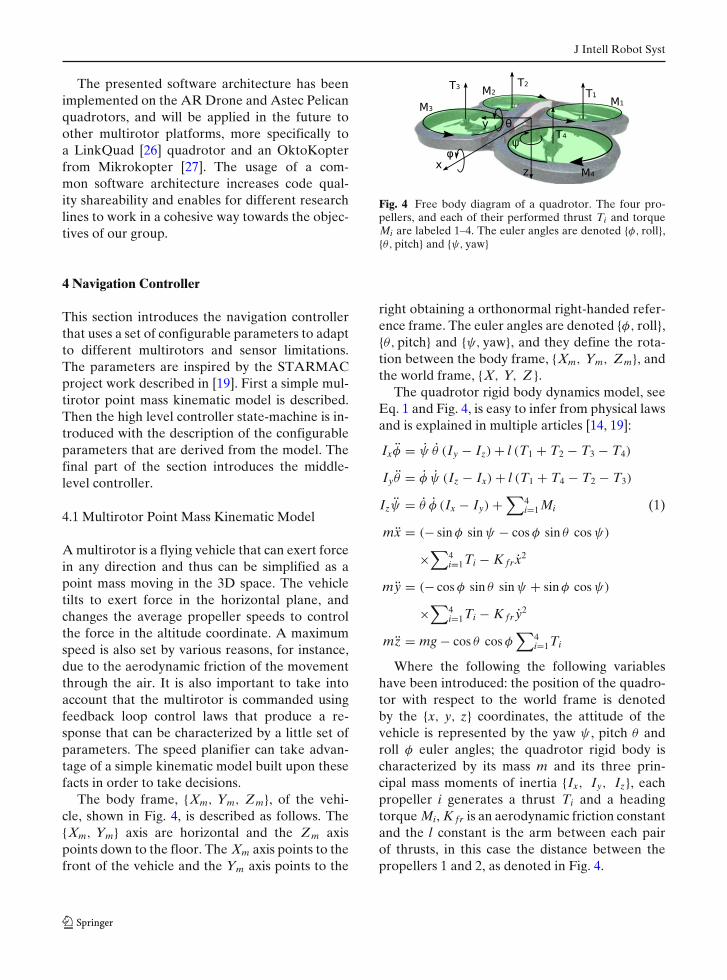
Fig. 4 Free body diagram of a quadrotor. The four pro-pellers, and each of their performed thrust Ti and torqueMi are labeled 1–4. The euler angles are denoted {φ, roll},{θ, pitch} and {ψ, yaw}
right obtaining a orthonormal right-handed refer-ence frame. The euler angles are denoted {φ, roll},{θ, pitch} and {ψ, yaw}, and they define the rota-tion between the body frame, {Xm, Ym, Zm}, andthe world frame, {X, Y, Z }.
The quadrotor rigid body dynamics model, seeEq. 1 and Fig. 4, is easy to infer from physical lawsand is explained in multiple articles [14, 19]:
Ixφ = ψ θ (Iy − Iz) + l (T1 + T2 − T3 − T4)
Iyθ = φ ψ (Iz − Ix) + l (T1 + T4 − T2 − T3)
Izψ = θ φ (Ix − Iy) +∑
4i=1 Mi (1)
mx = (− sin φ sin ψ − cos φ sin θ cos ψ)
×∑
4i=1Ti − K frx2
my = (− cos φ sin θ sin ψ + sin φ cos ψ)
×∑
4i=1Ti − K fr y2
mz = mg − cos θ cos φ∑
4i=1Ti
Where the following the following variableshave been introduced: the position of the quadro-tor with respect to the world frame is denotedby the {x, y, z} coordinates, the attitude of thevehicle is represented by the yaw ψ , pitch θ androll φ euler angles; the quadrotor rigid body ischaracterized by its mass m and its three prin-cipal mass moments of inertia {Ix, Iy, Iz}, eachpropeller i generates a thrust Ti and a headingtorque Mi, K fr is an aerodynamic friction constantand the l constant is the arm between each pairof thrusts, in this case the distance between thepropellers 1 and 2, as denoted in Fig. 4.
J Intell Robot Syst
The following control loops are usually imple-mented inside the autopilot board of the multi-rotor: the attitude (roll, φ, pitch, θ , and yaw, ψ)control loops and altitude, z, control loop. Theautopilot boards usually accept roll, pitch, yawspeed and altitude speed references. So that thesaturation bounds for these variables is set bythe autopilot board capabilities. Thus, it is onlyrequired to further develop the equations of mou-vement in the horizontal plane.
If the flight is performed at constant altitudethen,
∑4i=1 Ti ≈ mg, and taking the approximation
to low roll and pitch angles, then the equationsthat define the mouvement in the horizontal planeare derived from Eq. 1:
mx = (−θ cos ψ − φ sin ψ) mg − K frx2
my = (−θ sin ψ + φ cos ψ) mg − K fr y2 (2)
Two additional attitude variables are defined{φv, virtual roll}, {θv, virtual pitch}, which controlde position of the vehicle in the horizontal {X, Y}plane. They are related to the actual {φ, θ}through the yaw (ψ) angle as follows:
l[θv
φv
]=
[cos(ψ) sin(ψ)
− sin(ψ) cos(ψ)
] [θ
φ
](3)
The attitude controller (tr ≈ 200–300 ms) issignificantly faster than the horizontal speed loop(tr ≈ 1–2 s). This fact allows to correct the cou-pling introduced by the yaw commands in thehorizontal speed loops using the decoupling law,defined by Eq. 3. The reference frame changedefined by Eq. 3 is included in the controller, sothat the {φv, θv} can be used for the controllerdesign.
The dynamic model of the multirotor is muchsimpler when expressed using the virtual anglesand a maximum value for the quadrotor acceler-ation saturation can be infered from Eqs. 2 and 3as follows:
x ≈ −g θv − (K fr/m) x2 → |x|≤ g |θv max| − (K fr/m) x2 (4)
y ≈ g φv − (K fr/m) y2 → |y|≤ g |φv max| − (K fr/m) y2 (5)
The maximum horizontal speed of the vehicle,vxy max, is physically limited by the aerodynamicfriction. Thus, the maximum quadrotor speed isexpressed by Eq. 7 and the following model:(x2 + y2) ≤ v2
xy max (6)
The altitude acceleration can be modeled sim-ilarly, but the AR Drone only accepts altitudespeed commands; which is the reason to constrainthe altitude speed and not its acceleration:
|z| ≤ dzdt c max
(7)
The point mass model has to take into accountthat the vehicle is being commanded using feed-back control laws, and that the controller will notbe able to push the vehicle capabilities to thephysical limits stated above. Thus the following setof parameters is selected based on this fact and onthe previous considerations:
– The combination of Eqs. 7 and 6 set a maxi-mum speed on any direction.
– The speed response of the vehicle can be char-acterized by the response time of the speedcontrol loop trv max
– The maximum acceleration is physically lim-ited by Eqs. 4 and 5, and can be further de-termined by experimental tests. But the ac-tual accelerations obtained during trajectotrycontrol depend on the performances of thecontroller and on the smoothness of the speedreferences set to the speed control loop. Thus,the maximum acceleration parameters in thehorizontal plane are derived {ax max, ay max}.
– The trajectory around checkpoints can be ap-proximately modeled by a sector of circumfer-ence thus requiring a centripetal accelerationthat is limited by
ac xy ≤ g { θv max, φv max} = v2t
Rc(8)
where vt and Rc are the average speed andcurve radius during the turn.
4.2 Middle-Level Controller
The mid-level controller is shown in Fig. 5 andit is inpired on previous research from other

J Intell Robot Syst
Fig. 5 The middle-level controller architecture is a cascadecontroller, which consists of an inner speed loop and anouter position loop. The reference change block, whichimplements Eq. 3 ensures that the roll and pitch commandsare decoupled from the yaw heading. This allows for the
yaw command to be set independently from the positionand speed references. Thus, separating the left part of thediagram which is expressed in world coordinates, from theright part that is calculated in body frame coordinates
groups [13, 14, 19]. Its general architecture is acascade controller consisting of an inner speedloop and an outer position loop. But it also in-cludes control laws to take into account the overallsystem capabilities. Some characteristics of thecontrol architecture decipted in Fig. 5 are:
– The position controller loop only commandsachievable speeds to the speed controller loop,see left block in Fig. 5. The reference (feedfor-ward) speed along the trajectory is saturatedto vat max and vat z max; and the cross-track refer-ence speed is saturated to vct max and vct z max.Both speed limits are set so that vat max +vct max ≤ vxy max, vat z max + vct z max ≤ vz max.
– The planned along-track velocity {vat xc, vat yc,
vat zc} is lower than the maximum velocity,thus, giving the relative position controller aspeed margin to work on.
– The reference change block, which imple-ments Eq. 3 ensures that the roll and
pitch commands are decoupled from the yawheading.
– The aerodynamic friction is partially lin-earized, in the NLF blocks, using the inverseof the identified aerodynamic friction.
– In the PID modules the derivate action isfiltered to limit noise amplification and the in-tegral action features anti-windup saturation.
– The variables {θ f f , ψ f f } are feed-forwardcommands that are calculated by the statemachine using the planned acceleration andEqs. 4 and 5 without considering the aerody-namic friction.
4.3 High-Level Controller - State-Machine
The HL controller is implemented using a FiniteState Machine (FSM), which uses the state esti-mation from the EKF to calculate the mid-levelcontroller references. The FSM has three states

J Intell Robot Syst
corresponding to three control strategies: hover ina desired position, follow a straight segment of thetrajectory and turn to head to the next trajectorysegment. The work of the FSM is to navigate alonga waypoint trajectory, and it can be summarized asthe repetition of the following steps:
1. Follow the current straight segment, acceler-ating at first, and slowing down before reach-ing the next turn,
2. Perform the turn, controlling the speed direc-tion to achieve a soft alignment with the nextstraight segment.
Every time the controller output is calculated theFSM calculates the planned speed at the currentposition vplan(s):
1. The speed, {Vturn i}, inner turn angle at check-point, {αi}, and radius, {Rturn i}, during eachturn are precalculated each time the refer-ence trajectory is changed, either because thewhole trajectory is changed or because a way-point was added. The radius is calculated sothat the trajectory passes at a distance Rconf/2from the checkpoint, where Rconf is the maxi-mum distance at which the checkpoint is con-sidered to be reached. The planned speed foreach turn is selected either according to Eq. 8either considering that the turn requires astall-turn or turn-around maneuver, vstall turn,which corresponds to a planned speed nearzero.
2. The algorithm explained in Section 4.4 is usedto calculate the planned speed, vplan(s), at thecurrent position.
The FSM has also two additional operation modeswhere the quadrotor is controlled either only inposition control, or in speed control. These canbe used by the task scheduler to perform certaintasks.
The middle-level (ML) controller, see Fig. 3,receives position, { xc, yc, zc}, yaw heading, ψc,speed, {vat xc, vat yc, vat zc}, and tilt feed-forward,{θ f f , ψ f f }, commands from the FSM, as shownin Fig. 5. The presented controller, which is in-spired on those presented in [14, 19], allows touse single mid-level architecture for the three con-trol modes: trajectory, position and speed modes.
These references to the ML controller are calcu-lated by the FSM in such a way that the relativeposition and speed commands are orthogonal:
– The position references[xc, yc, zc
]are cal-
tulated projecting the estimated position [xest,
yest, zest] onto the reference trajectory.– The along-track speed commands, [ vat xc,
vat yc, vat zc], are parallel to the trajectoryvplan(s) utangent.
– The along-track speed commands, [ vat xc,
vat yc, vat zc], are derivated and smoothed us-ing a low-pass filter to obtain an accelerationcommand based on Eqs. 4 and 5, so that thefeed-forward attitude references,
{θ f f , φ f f
},
are calculated as follows:{θ f f , φ f f
} ={
−asin(
xm
g
), asin
(ym
g
)}
4.4 Speed Planner Algorithm
The planned speed depends on the current speedand position of the multirotor, and on the pre-vious and subsequent trajectory waypoints. Thespeed planner uses a uniform acceleration motionmodel to calculate both: the acceleration profilefrom the previous trajectory waypoints, and thedeceleration profile to perform the following turnssuccesfully. In addition to this model the speedloop response is modeled taking into account itsresponse time.
The algorithm calculates the following dis-tances for each of the neighbouring waypoints:
1. �dchk i, the distance to waypoint i from thecurrent estimated quadrotor position.
2. �dturn i = (Rturn i + Rconf2 ) sin(αi/2), the
distance to waypoint i when the turn isto be started; where Rconf is the waypointmaximum clearance distance, {Rturn i} is theplanned turn radius at waypoint i and {αi} isthe inner turn angle at waypoint i.
3. �dtrv i = trv max
√v2
x est + v2y est, the distance re-
quired by the speed loop to slow down, where{vx est, vy est} is the current estimated velocityand trv max is the speed loop response time.
Then the optimal speed for the neighbour-ing checkpoints, vplani
, is calculated depending
J Intell Robot Syst
on the sign of �d = (�dchk i − �dturn i − �dtrv i).
If �d ≥ 0 then vplani=
√V2
turn i + 2axy max �d, elseif �d < 0 then vplani
= Vturn i. Where {Vturn i} isthe planned speed at turn i. Finally the plannedspeed at the current position, vplan(s), is calcu-lated as the minimum of the precaltulated optimalspeeds vplan(s) = arg mini (vplani
). The coordinate sdenotes the position of the quadrotor along thetrajectory, and the expression vplan(s) highlightsthat the planned speed depends only on s and thefollowing set of configurable parameters.
4.5 Configurable Parameters Set
From the prior explanation the set of configurableparameters is derived:
– {vat max, vct max, vat z max, vct z max}, are the satu-ration speed limits used inside themiddle level controller that are imposed byeither the kinematic capabilities of the vehicle,or the measurement range of the onboardsensors or the precision requirements of thetask at hand.
– {Rconf, vstall turn, trv max, axy max}, are the para-meters that are used to determine the plannedspeed at each turn, {Vturn i}, and to calculatethe planned speed, vplan(s), at every controllerstep iteration.
5 Experimental Results
This section describes five separate experimentalflights that show the navigation capabilities ofthe presented system architecture. All the flightsare trajectory tracking tests in autonomous nav-igation carried out in an outdoors environment,simulating a GPS-denied situation. Thus, GPS wasunavailable and unsued during the tests. All theflights were performed with the AR Drone 2.0with the outdoors hull, but similar flights withother drones can be found in [3]. The flight tra-jectories are shown in Figs. 6, 7 and 8. The systemhas been tested following regular polygon trajec-tories on the XY plane, with varying altitude oneach waypoint, of values of 0–3 m higher thanthe first checkpoint’s altitude. A summary of the
−6−4
−20
2
02
46
8
−5−4−3
(a)
x [m]y [m]
z [m
]
position est.reference
−8−6
−4−2
02
02
46
810
−5−4−3
(b)
x [m]y [m]z
[m]
position est.referenceheading
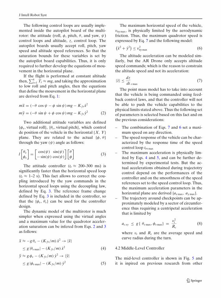
Fig. 6 Pseudo-square trajectory following experimentaltest on an outdoors environment performed using ourachitecture and an AR Drone 2.0. The a graph shows thereferece and followed trajectory in the XYZ space, andthe b graph additionally shows the vehicle heading duringthe second lap of the experiment were the yaw controllerinteraction with the trajectory following task was tested.The trajectory is a square on the XY plane with varying val-ues of altitude, on the 2.5–5.5 m range, at each checkpoint.The test consisted on three laps, where the yaw headingcontrol was tested on the second lap, which is plotted ongraph (b). Some performance parameters obtained fromthis test are shown in Table 1
controller performances in these tests is shown inTable 1.
The AR Drone 2.0 was configured with the fol-lowing parameters values. The maximum hori-zontal speed was set to 2.75 m/s, where vat max =2.0 m/s, vct max = 0.75 m/s. The FSM parameterswere set to Rconf = 0.25 m, vstall turn = 0.25 m/s,trv max = 1.20 s, and the maximum acceleration toaxy max = 0.70 m/s2. The configuration parameterswere selected to obtain high speeds on the straightsegments, with the objective of studying the con-troller performance on this configuration on out-doors environments.

J Intell Robot Syst
−10−5
0
0
5
10
−8
−6
(c)
x [m]y [m]
z [m
]position est.reference
−10−5
0
0
5
10
−8−7−6
(d)
x [m]y [m]
z [m
]
position est.referenceheading
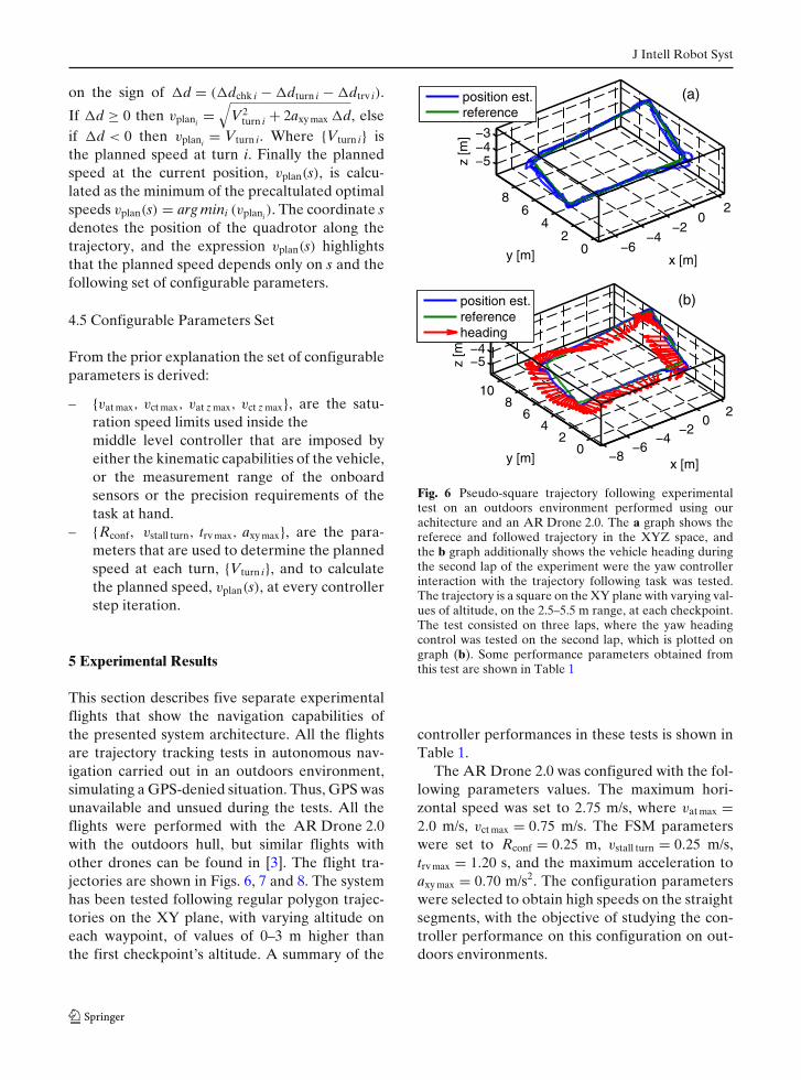
Fig. 7 Pseudo-hexagon trajectory following experimentaltest on an outdoors environment performed using ourachitecture and an AR Drone 2.0. The c graph shows thereferece and followed trajectory in the XYZ space, andthe d graph additionally shows the vehicle heading duringthe second lap of the experiment were the yaw controllerinteraction with the trajectory following task was tested.The trajectory is an hexagon on the XY plane with vary-ing values of altitude, on the 5.5–8.5 m range, at eachcheckpoint. The test consisted on three laps, where theyaw heading control was tested on the second lap, whichis plotted on graph (d). Some performance parametersobtained from this test are shown in Table 1
Each experiment is shown in one figure: thefirst experiment consisted of a pseudo-square tra-jectory shown on Fig. 6, the second one was apseudo-hexagon shown on Fig. 7, and the last onewas a pseudo octagon shown on Fig. 8. As shownthe drone follows a trajectory made out of straightsegments and circle segments around the corners.The first graphs {(a), (c) and (e)} show only thetrajectory reference and the estimated position,and the second ones {(b), (d) and (f)} show alsothe yaw heading during one of the laps. As can beappreciated from the graphs; the yaw control canbe handled separately from the position control.
−15−10
−50
0
5
10
15
−6−4
(e)
x [m]y [m]
z [m
]
position est.reference
−15−10
−50
05
1015
−6−4
(f)
x [m]y [m]
z [m
]
position est.referenceheading
Fig. 8 Pseudo-octagon trajectory following experimentaltest on an outdoors environment performed using ourachitecture and an AR Drone 2.0. The e graph shows thereferece and followed trajectory in the XYZ space, andthe f graph additionally shows the vehicle heading duringthe second lap of the experiment were the yaw controllerinteraction with the trajectory following task was tested.The trajectory is an octagon on the XY plane with varyingvalues of altitude, on the 3.0–6.0 m range, at each check-point. The test consisted on two laps, where the yaw head-ing control was tested on the second lap, which is plotted ongraph (f). The test was interrupted at the end of the secondlap due to poor WiFi performance. Some performanceparameters obtained from this test are shown in Table 1
The error to the trajectory is measured againstthe odometry based position estimation. As ex-pected this estimation is not accurate, and cum-mulates error over time. A ground truth to obtainan accurate tracking error is difficult to obtainwithout a motion capture system, which is thereason why it is not calculated. The drift dependson many circumstances that affect the quality ofthe optical flow speed estimation: texture of thefloor, size of identifiable features in floor texture,illumination, altitude of the flight, yaw rotationspeed, etc. To keep a good quality on the positionmeasurements the yaw rotation speed commands

J Intell Robot Syst
Table 1 Summary of results of the experimental testsobtained for the trajectories presented on the paper onFigs. 6, 7 and 8
Parameter dmean dmax vmean vmax �Lmean �ttest
units [m] [m] [m/s] [m/s] [m] [s]
Square 0.17 0.70 0.92 1.90 7.72 123.0Hexagon 0.31 1.71 1.09 1.95 7.75 123.0Octagon 0.32 2.90 1.17 2.10 7.75 95.0
The specified parameters are: average, dmean, and maxi-mum, dmax, tracking error; average, vmean, and maximum,vmax, speed along-trajectory; �Lmean , mean distance be-tween waypoints and �ttest, duration of the test. The testedtrajectories and poligons on the XY plane, with varyingvalues of altitude on each waypoint. The tracking erroris calculated from the odometry based position estimates.The mean and maximum speed are calculated taking intoaccount the component along the trajectory, where thenumber of laps on each test was 2–3 laps
are saturated at 50◦/s, and are usually below 30◦/s.The flights were mostly anaffected during yawheading rotation. In the flights exposed in thissection the yaw rotation speed attained valuesof about 30–50◦/s. The experimental data clarify,however, that the vehicle tends to oscillate aroundthe reference trajectory during the yaw rotation.High yaw rotation speeds do affect the positioncontrol, but 50◦/s is an acceptable value for manyapplications.
The altitude on each experiment was 2.5–5.5 m,5.5–8.5 m and 3.0–6.0 m respectively. The ARDrone 2.0 can measure altitude precisely of up to6 m [1] using the ultrasound sensor. For higheraltitudes the drone has to switch to using thepressure sensor. In practice, the drone telemetrywill show a good tracking on the altitude coordi-nate, while on reality the vehicle is correcting thealtitude internally moving upwards or downwards.This was specially appreciable during some ofthe experiments shown on this paper, but is notvisible on the plots because the sensor reading ismisleading.
The selected tests show how our architectureis able to deal with moderate winds and how ittakes into account automatically the curve innerangles of the trajectory at each waypoint. Thetrajectories have a varying number of waypointsto provide a varying inside angle of the trajec-tory at their waypoints. Since they are all regular
polygons on the XY plane, then the higher thenumber of waypoints the bigger the inner an-gles of the trajectory will be, allowing for fasterpasses through them. This is appreciated by themean speed during trajectory tracking, see vmean inTable 1. The other factor that affectes the max-imum and mean speeds, vmax and vmean respec-tively, is the distance between waypoints; but allthe trajectories where performed with similar dis-tances. Longer distances between waypoints allowthe multirotor to accelerate to and decceleratefrom higher speeds.
In some occasions, the drone drifts off coursein the curves of the trajectory. But this behaviouris not deterministic and the same error is notcommited in every corner and is not even repeatedon the next lap. However, it could be avoidedlowering the axy max and trv max to more restrictivevalues. It would al be convenient to have sepa-rate values of acceleration for the curves and thestraight lines, as the controller architecture doesnot perform equally well on straight trajectorysegments than in the curves. Then the solutionsare improving the controller, or adding parame-ters to the speed planning algorithm to take intoaccount this issue. Another occasional behaviouris that the odometry error may increase substa-nially and the drone might perform a 20–50% big-ger trajectory than commanded, due to odometryestimation errors; or subsequentelly cummulatea constant drift per lap on a certain direction.This behaviour might be triggered by the ARDrone’s altitude sensor switching solution, but wedo not have experimental evidence to ascertainthe source of this occasional problem.
6 Conclusions
In this paper, we have extended the experimen-tal work presented on a previous conference pa-per [3], to outdoors environments performing 3Dtrajectories using an additional multirotor, theAR Drone 2.0 with its outdoors hull. The testswith AR Drone 2.0 showed that this controlleris able to handle wind disturbances accumulat-ing small tracking error. However, our architec-ture requires a good odometry sensor which in

J Intell Robot Syst
the presented work is directly provided by theAR Drone 2.0’s hardware.
We presented our experimental work on thedesign of a multirotor navigation controller thatallows for safer multirotor flights. The contribu-tion of these works is two-fold: first, a discussionon various causes for multirotor navigation con-trollers malfunctioning is presented. Second, wederived a simple and robuts approach to addressthese causes natively in our middle-level con-troller architecture. As a further contributionto the research community, all the code re-lated to this paper will be available on GitHubrepositories.
This work is centered around the fact that thestate estimation algorithms and the controller caninteract in a very negative way when visual odom-etry estimations are faulty. This motivated ourwork to identify its causes and design an approachto overcome the problem. Our experimental workhas led us to identify the safety boundaries underwhich our estimation algorithms work correctly.Then, our controller was designed to nativelyallow the saturation of the vehicle velocity. Al-though the speed can be saturated on the tra-jectory planning module, introducing this featurenatively on the controller also allows to fly safelyon speed and position control modes, or wheneverthe middle-level controller is utilized. The workhas resulted in an overall increase of the safetyand repeatibility of our experimental tests, whichin turn allowed us to increase our test’s efficiencyand gain two awards on the IMAV 2012 compe-tition. The experimental tests on our multirotorplatforms have shown the robustness of our ap-proach. The small trajectory tracking errors, mea-sured against the EKF estimation, on these testsshow that our efforts should be focused on im-proving our odometry and localization algorithmsrather than the controller itself.
As an overall summary, the presented architec-ture was developed to allow a fast implementationon multiple multirotor vehicles. It permits to testthe autonomous navigation software during realflight with a low cost vehicle, such as an ARDrone, and then easily make it portable to a moreprofessional vehicle, such as an Asctec Pelican.The paper highlights the usage of a common drone
model, and the issues that had to be solved toattain portability among multiple platforms. Asfuture work, our group is interested on visuallocalization algorithms that can improve odome-try and position measurements to the EKF; andthe presented controller architecture will be testedin outdoors adding the GPS measurements forcivilian applications research.
Acknowledgements The work reported in this article isthe consecution of several research stages at the ComputerVision Group—Universidad Politécnica de Madrid. Thiswork was supported by the Spanish Science and Tech-nology Ministry under the grant CICYT DPI2010-20751-C02-01, and the following institutions by their scholarshipgrants: CSIC-JAE, CAM and the Chinese ScholarshipCouncil. All the authors are with the Computer VisionGroup, www.vision4uav.eu, which belongs to the Centrefor Automation and Robotics, joint research center fromthe Spanish National Research Council (CSIC) and thePolytechnic University of Madrid (UPM).
References
1. The Navigation and Control Technology Inside theAR.Drone Micro UAV. Milano, Italy (2011)
2. Pestana, J.: On-board control algorithms for quadro-tors and indoors navigation. Master’s thesis, Universi-dad Politécnica de Madrid, Spain (2012)
3. Pestana, J., Mellado-Bataller, I., Fu, C., Sanchez-Lopez, J.L., Mondragon, I.F., Campoy, P.: A gen-eral purpose configurable navigation controller for mi-cro aerial multirotor vehicles. In: 2013 InternationalConference on Unmanned Aircraft Systems (ICUAS),pp. 557–564 (2013)
4. Honegger, D., Meier, L., Tanskanen, P., Pollefeys, M.:An open source and open hardware embedded metricoptical flow CMOS camera for indoor and outdoorapplications. In: International Conference on Roboticsand Automation ICRA 2013 (2013)
5. Zingg, S., Scaramuzza, D., Weiss, S., Siegwart, R.:MAV navigation through indoor corridors using opti-cal flow. In: 2010 IEEE International Conference onRobotics and Automation (ICRA) (2010)
6. Zufferey, J.-C., Beyeler, A., Floreano, D.: Au-tonomous flight at low altitude with vision-based col-lision avoidance and GPS-based path following. In:Proceedings of the IEEE International Conferenceon Robotics and Automation (ICRA), IEEE. Onlineavailable: http://icra2010.grasp.upenn.edu/ (2010)
7. Lippiello, V., Loianno, G., Siciliano, B.: MAV indoornavigation based on a closed-form solution for absolutescale velocity estimation using optical flow and iner-tial data. In: 2011 50th IEEE Conference on Decision

J Intell Robot Syst
and Control and European Control Conference (CDC-ECC), pp. 3566–3571 (2011)
8. Conroy, J., Gremillion, G., Ranganathan, B., Humbert,J.S.: Implementation of wide-field integration of op-tic flow for autonomous quadrotor navigation. Auton.Robot. 27(3), 189–198 (2009)
9. Mellado Bataller, I.: A new framework for interfac-ing with MAVs. https://github.com/uavster/mavwork(2012). Accessed 7 June 2013
10. Pestana, J.: A general purpose multirotor controllercompatible with multiple multirotor vehicles andwith the mavwork open-source project. https://github.com/jespestana/MultirotorController4mavwork (2013).Accessed 24 Apr 2013
11. A ros stack open-source implementation of the gen-eral purpose multirotor controller compatible the ardrone 1 & 2, it has been tested succesfully on theasctec pelican but integration is not provided on thisversion of the code. https://github.com/jespestana/ros_multirotor_navigation_controller (2013)
12. Motion capture systems from vicon. http://www.vicon.com/ (2013). Accessed 10 Sept 2013
13. Mellinger, D., Michael, N., Kumar, V.: Trajectory gen-eration and control for precise aggressive maneuverswith quadrotors. In: Int Symposium on ExperimentalRobotics, (2010)
14. Michael, N., Mellinger, D., Lindsey, Q.: The GRASPmultiple micro UAV testbed. IEEE Robot. Autom.Mag. 17(3), 56–65 (2010)
15. Lupashin, S., Schollig, A., Sherback, M., D’Andrea,R.: A simple learning strategy for high-speed quadro-copter multi-flips. In: 2010 IEEE International Con-ference on Robotics and Automation (ICRA 2010),pp. 1642–1648 (2010)
16. Kushleyev, A., Kumar, V., Mellinger, D.: Towardsa swarm of agile micro quadrotors. In: Proceedingsof Robotics: Science and Systems. Sydney, Australia(2012)
17. Schölling, A., Augugliaro, F., Lupashin, S., D’Andrea,R.: Synchronizing the motion of a quadrocopter tomusic. In: IEEE International Conference on Roboticsand Automation ICRA, pp. 3355–3360. Onlineavailable: http://ieeexplore.ieee.org/xpls/abs_all.jsp?arnumber=5509755 (2010)
18. The Stanford/Berkeley Testbed of Autonomous Ro-torcraft for Multi-Agent Control (STARMAC) project.
http://hybrid.eecs.berkeley.edu/starmac/ (2013). Accessed10 Sept 2013
19. Hoffmann, G.M., Waslander, S.L., Tomlin, C.J.:Quadrotor helicopter trajectory tracking control. In:AIAA Guidance, Navigation and Control Confer-ence and Exhibit, Honolulu, Hawaii, USA, August2008
20. Hoffmann, G., Waslander, S., Tomlin, C.: Aerodynam-ics and control of autonomous quadrotor helicopters inaggressive maneuvering. In: 2009 IEEE InternationalConference on Robotics and Automation, pp. 3277–3282. IEEE (2009)
21. Gillula, J.H., Huang, H., Vitus, M.P., Tomlin, C.J.:Design of guaranteed safe maneuvers using reachablesets: autonomous quadrotor aerobatics in theory andpractice. In: Proc. of the IEEE Int. Conf. on Roboticsand Automation, Anchorage, AK, May 2010, pp. 1649–1654
22. Rudol, P., Wzorek, M., Conte, G., Doherty, P.: Microunmanned aerial vehicle visual servoing for coopera-tive indoor exploration. In: 2008 IEEE Conference onAerospace (2008)
23. International micro air vehicle conference and flightcompetition IMAV 2012, program informationfor flight competition brochure. http://www.dgon-imav.org/3.0.html#c214 (2013). Accessed 10 Sept 2013
24. Mellado-Bataller, I., Mejias, L., Campoy, P., Olivares-Mendez, M.A.: Rapid prototyping framework for vi-sual control of autonomous micro aerial vehicles.In: 12th International Conference on Intelligent Au-tonomous System (IAS-12), Jeju Island, Korea. Onlineavailable: http://eprints.qut.edu.au/50709/ (2012)
25. Mellado-Bataller, I., Pestana, J., Olivares-Mendez,M.A., Campoy, P., Mejias, L.: MAVwork: a frame-work for unified interfacing between micro aerialvehicles and visual controllers. Frontiers of Intelli-gent Autonomous Systems Studies in ComputationalIntelligence, vol. 466, pp. 165–179. Online available:http://link.springer.com/chapter/10.1007%2F978-3-642-35485-4_13 (2013)
26. UAS Technologies Sweden AB, LinkQuad quadrotorwebsite. http://uastech.com/platforms.htm (2013). Ac-cessed 10 Sept 2013
27. MikroKopter, OktoKopter multirotor website. http://www.mikrokopter.de/ucwiki/en/MK-Okto (2013). Ac-cessed 10 Sept 2013