a general framework for a class of first …eesser/papers/esser_zhang_chan_rerevised.pdf · a...

A GENERAL FRAMEWORK FOR A CLASS OF FIRST ORDERPRIMAL-DUAL ALGORITHMS FOR CONVEX OPTIMIZATION IN

IMAGING SCIENCE

ERNIE ESSER XIAOQUN ZHANG TONY CHAN

Abstract. We generalize the primal-dual hybrid gradient (PDHG) algorithm proposed by Zhuand Chan in [M. Zhu, and T. F. Chan, An Efficient Primal-Dual Hybrid Gradient Algorithm forTotal Variation Image Restoration, UCLA CAM Report [08-34], May 2008] to a broader class ofconvex optimization problems. In addition, we survey several closely related methods and explainthe connections to PDHG. We point out convergence results for a modified version of PDHG thathas a similarly good empirical convergence rate for total variation (TV) minimization problems. Wealso prove a convergence result for PDHG applied to TV denoising with some restrictions on thePDHG step size parameters. It is shown how to interpret this special case as a projected averagedgradient method applied to the dual functional. We discuss the range of parameters for which thesemethods can be shown to converge. We also present some numerical comparisons of these algorithmsapplied to TV denoising, TV deblurring and constrained l1 minimization problems.

Key words. convex optimization, total variation minimization, primal-dual methods, operatorsplitting, l1 basis pursuit

AMS subject classifications. 90C25, 90C06, 49K35, 49N45, 65K10

1. Introduction. Total variation minimization problems arise in many imageprocessing applications for regularizing inverse problems where one expects the re-covered image or signal to be piecewise constant or have sparse gradient. However, alack of differentiability makes minimizing TV regularized functionals computationallychallenging, and so there is considerable interest in efficient algorithms, especiallyfor large scale problems. More generally, there is interest in practical methods forsolving non-differentiable convex optimization problems, TV minimization being animportant special case.

The PDHG algorithm [58] in a general setting is a method for solving problemsof the form

minu∈Rm

J(Au) + H(u),

where J and H are closed proper convex functions and A ∈ Rn×m. Usually, J(Au)

will correspond to a regularizing term of the form ‖Au‖, in which case the PDHGmethod works by using duality to rewrite it as the saddle point problem

minu∈Rm

max‖p‖∗≤1

〈p, Au〉 + H(u)

and then alternating dual and primal steps of the form

pk+1 = arg max‖p‖∗≤1

〈p, Auk〉 − 1

2δk

‖p − pk‖22

uk+1 = arg minu∈Rm

〈pk+1, Au〉 + H(u) +1

2αk

‖u − uk‖22

for appropriate parameters αk and δk. Here, ‖ · ‖ denotes an arbitrary norm on Rn

and ‖ · ‖∗ denotes its dual norm defined by

‖x‖∗ = max‖y‖≤1

〈x, y〉,

1

2 E. Esser, X. Zhang and T.F. Chan

where 〈·, ·〉 is the standard Euclidean inner product. Formulating the saddle pointproblem used the fact that ‖ · ‖∗∗ = ‖ · ‖ [32], from which it follows that ‖Au‖ =max‖p‖∗≤1〈p, Au〉.

PDHG can also be applied to more general convex optimization problems. How-ever, its performance for problems like TV denoising is of special interest since itcompares favorably with other popular methods. An adaptive time stepping schemefor PDHG was proposed in [58] and shown to outperform other popular TV denois-ing algorithms like Chambolle’s method [10], the method of Chan, Golub and Mulet(CGM) [13], FTVd [54] and split Bregman [29] in many numerical experiments witha wide variety of stopping conditions. Aside from some special cases of the PDHG al-gorithm like gradient projection and subgradient descent, the theoretical convergenceproperties were not known.

PDHG is an example of a first order method, meaning it only requires functionaland gradient evaluations. Other examples of first order methods popular for TV min-imization include gradient descent, Chambolle’s method, FTVd and split Bregman.Second order methods like CGM and semismooth Newton approaches [30, 31, 17]work by essentially applying Newton’s method to an appropriate formulation of theoptimality conditions and therefore also require information about the Hessian. Thisusually requires some smoothing of the objective functional. These methods can besuperlinearly convergent and are therefore useful for computing benchmark solutionsof high accuracy. However, the cost per iteration is usually higher, so for large scaleproblems or when high accuracy is not required, these are often less practical thanthe first order methods that have much lower cost per iteration. Here, we will focuson a class of first order methods related to PDHG that are simple to implement andcan also be directly applied to non-differentiable functionals.

PDHG is also an example of a primal-dual method. Each iteration updates botha primal and a dual variable. It is thus able to avoid some of the difficulties that arisewhen working only on the primal or dual side. For example, for TV minimization,gradient descent applied to the primal functional has trouble where the gradient ofthe solution is zero because the functional is not differentiable there. Chambolle’smethod is a method on the dual that is very effective for TV denoising, but doesn’teasily extend to applications where the dual problem is more complicated, such asTV deblurring. Primal-dual algorithms can avoid to some extent these difficulties.Other examples include CGM, the semismooth Newton approaches mentioned above,split Bregman, and more generally other Bregman iterative algorithms [57, 55, 53]and Lagrangian-based methods.

In this paper we show that we can make a small modification to the PDHGalgorithm, which has little effect on its performance, but that allows the modifiedalgorithm to be interpreted as a special case of a split inexact Uzawa method thatis analyzed and shown to converge in [56]. After initially preparing this paper itwas brought to our attention that the specific modified PDHG algorithm appliedhere has been previously proposed by Pock, Cremers, Bischof and Chambolle [40] forminimizing the Mumford-Shah functional. In [40] they also prove convergence fora special class of saddle point problems. In recent preprints [11, 12] that appearedduring the review process, this convergence argument has been generalized and givesa stronger statement of the convergence of the modified PDHG algorithm for thesame range of fixed parameters. Chambolle and Pock also provide a convergence rateanalysis in [12]. While the modified PDHG method with fixed step sizes is nearly aseffective as fixed parameter versions of PDHG, well chosen adaptive step sizes can

Primal-Dual Algorithms for Convex Optimization in Imaging Science 3

improve the rate of convergence. It’s proven in [12] that certain adaptive step sizeschemes accelerate the convergence rate of the modified PDHG method in cases whenthe objective functional has additional regularity. With more restrictions on the stepsize parameters, we prove a convergence result for the original PDHG method appliedto TV denoising by interpreting it as a projected averaged gradient method on thedual.

We additionally show that the modified PDHG method can be applied in the sameways PDHG was extended in [58] to apply to additional problems like TV deblurring,l1 minimization and constrained minimization problems. For these applications wepoint out the range of parameters for which the convergence theory is applicable.

Another contribution of this paper is to describe a general algorithm frameworkfrom the perspective of PDHG that explains the close connections between it, modifiedPDHG, split inexact Uzawa and more classical methods including proximal forwardbackward splitting (PFBS) [34, 39, 15], alternating minimization algorithm (AMA)[49], alternating direction method of multipliers (ADMM) [25, 27, 6] and DouglasRachford splitting [18, 24, 26, 19, 20]. These connections provide some additionalinsight about where PDHG and modified PDHG fit relative to existing methods.

The organization of this paper is as follows. In Section 2, we discuss primal-dualformulations for a general problem. We define a general version of PDHG and discussin detail the framework in which it can be related to other similar algorithms. Theseconnections are diagrammed in Figure 2.1. In Section 3 we define a discretizationof the total variation seminorm and review the details about applying PDHG to TVdeblurring type problems. In Section 4 we show how to interpret PDHG applied toTV denoising as a projected averaged gradient method on the dual and present aconvergence result for a special case. Then in Section 5, we discuss the applicationof the modified PDHG algorithm to constrained TV and l1 minimization problems.Section 6 presents numerical experiments for TV denoising, constrained TV deblurringand constrained l1 minimization, comparing the performance of the modified PDHGalgorithm with other methods.

2. General Algorithm Framework . In this section we consider a generalclass of problems that PDHG can be applied to. We define equivalent primal, dualand several primal-dual formulations. We also place PDHG in a general frameworkthat connects it to other related alternating direction methods applied to saddle pointproblems.

2.1. Primal-Dual Formulations. PDHG can more generally be applied towhat we will refer to as the primal problem

minu∈Rm

FP (u), (P)

where

FP (u) = J(Au) + H(u), (2.1)

A ∈ Rn×m, J : R

n → (−∞,∞] and H : Rm → (−∞,∞] are closed proper convex

functions. Assume there exists a solution u∗ to (P). So that we can use Fenchel duality([43] 31.2.1) later, also assume there exists u ∈ ri(domH) such that Au ∈ ri(domJ),which is almost always true in practice. When J was a norm, it was shown how touse the dual norm to define a saddle point formulation of (P) as

minu∈Rm

max‖p‖∗≤1

〈Au, p〉 + H(u).


This can equivalently be written in terms of the Legendre-Fenchel transform, or convexconjugate, of J denoted by J∗ and defined by

J∗(p) = supw∈Rn

〈p, w〉 − J(w).

When J is a closed proper convex function, we have that J∗∗ = J [21]. Therefore,

J(Au) = supp∈Rn

〈p, Au〉 − J∗(p).

So an equivalent saddle point formulation of (P) is

minu∈Rm

supp∈Rn

LPD(u, p), (PD)

where

LPD = 〈p, Au〉 − J∗(p) + H(u). (2.2)

This holds even when J is not a norm, but in the case when J(w) = ‖w‖, we can thenuse the dual norm representation of ‖w‖ to write

J∗(p) = supw

〈p, w〉 − max‖y‖∗≤1

〈w, y〉

=

{

0 if ‖p‖∗ ≤ 1

∞ otherwise,

in which case we can interpret J∗ as the indicator function for the unit ball in thedual norm.

Let (u∗, p∗) be a saddle point of LPD. In particular, this means

maxp∈Rn

〈p, Au∗〉 − J∗(p) + H(u∗) = LPD(u∗, p∗) = minu∈Rm

〈p∗, Au〉 + H(u) − J∗(p∗),

from which we can deduce the equivalent optimality conditions and then use thedefinitions of the Legendre transform and subdifferential to write these conditions intwo ways

−AT p∗ ∈ ∂H(u∗) ⇔ u∗ ∈ ∂H∗(−AT p∗) (2.3)

Au∗ ∈ ∂J∗(p∗) ⇔ p∗ ∈ ∂J(Au∗), (2.4)

where ∂ denotes the subdifferential. The subdifferential ∂F (x) of a convex functionF : R

m → (−∞,∞] at the point x is defined by the set

∂F (x) = {q ∈ Rm : F (y) ≥ F (x) + 〈q, y − x〉 ∀y ∈ R

m}.

Another useful saddle point formulation that we will refer to as the split primalproblem is obtained by introducing the constraint w = Au in (P) and forming theLagrangian

LP (u, w, p) = J(w) + H(u) + 〈p, Au − w〉. (2.5)

The corresponding saddle point problem is

maxp∈Rn

infu∈Rm,w∈Rn

LP (u, w, p). (SPP)


Although p was introduced in (2.5) as a Lagrange multiplier for the constraint Au = w,it has the same interpretation as the dual variable p in (PD). It follows immediatelyfrom the optimality conditions that if (u∗, w∗, p∗) is a saddle point for (SPP), then(u∗, p∗) is a saddle point for (PD).

The dual problem is

maxp∈Rn

FD(p), (D)

where the dual functional FD(p) is a concave function defined by

FD(p) = infu∈Rm

LPD(u, p) = infu∈Rm

〈p, Au〉−J∗(p)+H(u) = −J∗(p)−H∗(−AT p). (2.6)

Note that this is equivalent to defining the dual by

FD(p) = infu∈Rm,w∈Rn

LP (u, w, p). (2.7)

Since we assumed there exists an optimal solution u∗ to the convex problem (P), itfollows from Fenchel duality ([43] 31.2.1) that there exists an optimal solution p∗ to(D) and FP (u∗) = FD(p∗). Moreover, u∗ solves (P) and p∗ solves (D) if and only if(u∗, p∗) is a saddle point of LPD(u, p) ([43] 36.2).

By introducing the constraint y = −AT p in (D) and forming the correspondingLagrangian

LD(p, y, u) = J∗(p) + H∗(y) + 〈u,−AT p − y〉, (2.8)

we obtain yet another saddle point problem,

maxu∈Rm

infp∈Rn,y∈Rm

LD(p, y, u), (SPD)

which we will refer to as the split dual problem. Although u was introduced in(SPD) as a Lagrange multiplier for the constraint y = −AT p, it actually has the sameinterpretation as the primal variable u in (P). Again, it follows from the optimalityconditions that if (p∗, y∗, u∗) is a saddle point for (SPD), then (u∗, p∗) is a saddlepoint for (PD). Note also that

FP (u) = − infp∈Rn,y∈Rm

LD(p, y, u).

2.2. Algorithm Framework and Connections to PDHG . In this sectionwe define a general version of PDHG applied to (PD) and discuss connections torelated algorithms that can be interpreted as alternating direction methods appliedto (SPP) and (SPD). These connections are summarized in Figure 2.1.

The main tool for drawing connections between the algorithms in this section isthe Moreau decomposition [35, 15].

Theorem 2.1. [15] If J is a closed proper convex function on Rm and f ∈ R

m,then

f = arg minu

J(u) +1

2α‖u − f‖2

2 + α arg minp

J∗(p) +α

2‖p − f

α‖22. (2.9)

It was shown in [58] that PDHG applied to TV denoising can be interpreted asa primal-dual proximal point method applied to a saddle point formulation of theproblem. More generally, applied to (PD) it yields


Algorithm: PDHG on (PD)

pk+1 = arg maxp∈Rn

−J∗(p) + 〈p, Auk〉 − 1

2δk

‖p − pk‖22 (2.10a)


H(u) + 〈AT pk+1, u〉 +1

2αk

‖u − uk‖22, (2.10b)

where p0, u0 are arbitrary, and αk, δk > 0.

2.2.1. Proximal Forward Backward Splitting: Special Cases of PDHG. Two notable special cases of PDHG are αk = ∞ and δk = ∞. These special casescorrespond to the proximal forward backward splitting method (PFBS) [34, 39, 15]applied to (D) and (P) respectively.

PFBS is an iterative splitting method that can be used to find a minimum ofa sum of two convex functionals by alternating a (sub)gradient descent step with aproximal step. Applied to (D) it yields

pk+1 = arg minp∈Rn

J∗(p) +1

2δk

‖p − (pk + δkAuk+1)‖22, (2.11)

where uk+1 ∈ ∂H∗(−AT pk). Since uk+1 ∈ ∂H∗(−AT pk) ⇔ −AT pk ∈ ∂H(uk+1),which is equivalent to


H(u) + 〈AT pk, u〉,

(2.11) can be written as

Algorithm: PFBS on (D)


H(u) + 〈AT pk, u〉 (2.12a)


J∗(p) + 〈p,−Auk+1〉 +1

2δk

‖p − pk‖22. (2.12b)

Even though the order of the updates is reversed relative to PDHG, since the initial-ization is arbitrary it is still a special case of (2.10) where αk = ∞.

If we assume that J(·) = ‖ · ‖, we can interpret the pk+1 step as an orthogonalprojection onto a convex set,

pk+1 = Π{p:‖p‖∗≤1}

(

pk + δkAuk+1)

.

Then PFBS applied to (D) can be interpreted as a (sub)gradient projection algorithm.As a special case of ([15] Theorem 3.4), the following convergence result applies

to (2.12).Theorem 2.2. Fix p0 ∈ R

n, u0 ∈ Rm and let (uk, pk) be defined by (2.12). If H∗

is differentiable, ∇(H∗(−AT p)) is Lipschitz continuous with Lipschitz constant equalto 1

β, and 0 < inf δk ≤ sup δk < 2β, then {pk} converges to a solution of (D) and

{uk} converges to the unique solution of (P).


Proof. Convergence of {pk} to a solution of (D) follows from ([15] 3.4). From(2.12a), uk+1 satisfies −AT pk ∈ ∂H(uk+1), which, from the definitions of the subd-ifferential and Legendre transform, implies that uk+1 = ∇H∗(−AT pk). So by con-tinuity of ∇H∗, uk → u∗ = ∇H∗(−AT p∗). From (2.12b) and the convergence of{pk}, Au∗ ∈ ∂J∗(p∗). Therefore (u∗, p∗) satisfies the optimality conditions (2.3,2.4)for (PD), which means u∗ solves (P) ([43] 31.3). Uniqueness follows from the assump-tion that H∗ is differentiable, which by ([43] 26.3) means that H(u) in the primalfunctional is strictly convex.

It will be shown later in Section 2.2.3 how to equate modified versions of thePDHG algorithm with convergent alternating direction methods, namely split inexactUzawa methods from [56] applied to the split primal (SPP) and split dual (SPD)problems. The connection there is very similar to the equivalence from [49] betweenPFBS applied to (D) and what Tseng in [49] called the alternating minimizationalgorithm (AMA) applied to (SPP). AMA applied to (SPP) is an alternating directionmethod that alternately minimizes first the Lagrangian LP (u, w, p) with respect tou and then the augmented Lagrangian LP + δk

2 ‖Au − w‖22 with respect to w before

updating the Lagrange multiplier p.

Algorithm: AMA on (SPP)


H(u) + 〈AT pk, u〉 (2.13a)

wk+1 = arg minw∈Rn

J(w) − 〈pk, w〉 +δk

2‖Auk+1 − w‖2

2 (2.13b)

pk+1 = pk + δk(Auk+1 − wk+1) (2.13c)

To see the equivalence between (2.12) and (2.13), first note that (2.13a) is identicalto (2.12a), so it suffices to show that (2.13b) and (2.13c) are together equivalent to(2.12b). Combining (2.13b) and (2.13c) yields

pk+1 = (pk + δkAuk+1) − δk arg minw

J(w) +δk

2‖w − (pk + δkAuk+1)

δk

‖22.

By the Moreau decomposition (2.9), this is equivalent to

pk+1 = arg minp

J∗(p) +1

2δk

‖p − (pk + δkAuk+1)‖22,

which is exactly (2.12b).

In [49], convergence of (uk, wk, pk) satisfying (2.13) to a saddle point of LP (u, w, p)is directly proved under the assumption that H is strongly convex, an assumption thatdirectly implies the condition on H∗ in Theorem 2.2.

The other special case of PDHG where δk = ∞ can be analyzed in a similarmanner. The corresponding algorithm is PFBS applied to (P),


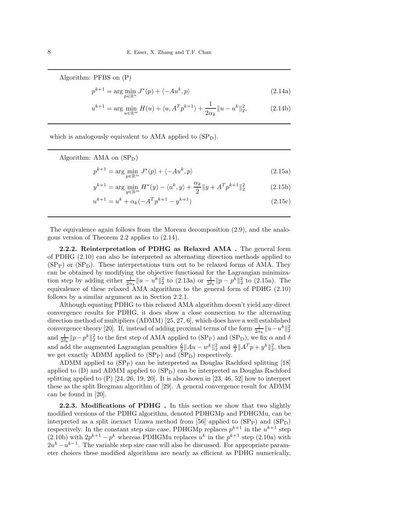
Algorithm: PFBS on (P)


J∗(p) + 〈−Auk, p〉 (2.14a)


H(u) + 〈u, AT pk+1〉 +1

2αk

‖u − uk‖22, (2.14b)

which is analogously equivalent to AMA applied to (SPD).

Algorithm: AMA on (SPD)

pk+1 = arg minp∈Rm

J∗(p) + 〈−Auk, p〉 (2.15a)

yk+1 = arg miny∈Rm

H∗(y) − 〈uk, y〉 +αk

2‖y + AT pk+1‖2

2 (2.15b)

uk+1 = uk + αk(−AT pk+1 − yk+1) (2.15c)

The equivalence again follows from the Moreau decomposition (2.9), and the analo-gous version of Theorem 2.2 applies to (2.14).

2.2.2. Reinterpretation of PDHG as Relaxed AMA . The general formof PDHG (2.10) can also be interpreted as alternating direction methods applied to(SPP) or (SPD). These interpretations turn out to be relaxed forms of AMA. Theycan be obtained by modifying the objective functional for the Lagrangian minimiza-tion step by adding either 1

2αk‖u − uk‖2

2 to (2.13a) or 12δk

‖p − pk‖22 to (2.15a). The

equivalence of these relaxed AMA algorithms to the general form of PDHG (2.10)follows by a similar argument as in Section 2.2.1.

Although equating PDHG to this relaxed AMA algorithm doesn’t yield any directconvergence results for PDHG, it does show a close connection to the alternatingdirection method of multipliers (ADMM) [25, 27, 6], which does have a well establishedconvergence theory [20]. If, instead of adding proximal terms of the form 1

2αk‖u−uk‖2

2

and 12δk

‖p−pk‖22 to the first step of AMA applied to (SPP) and (SPD), we fix α and δ

and add the augmented Lagrangian penalties δ2‖Au− wk‖2

2 and α2 ‖AT p + yk‖2

2, thenwe get exactly ADMM applied to (SPP) and (SPD) respectively.

ADMM applied to (SPP) can be interpreted as Douglas Rachford splitting [18]applied to (D) and ADMM applied to (SPD) can be interpreted as Douglas Rachfordsplitting applied to (P) [24, 26, 19, 20]. It is also shown in [23, 46, 52] how to interpretthese as the split Bregman algorithm of [29]. A general convergence result for ADMMcan be found in [20].

2.2.3. Modifications of PDHG . In this section we show that two slightlymodified versions of the PDHG algorithm, denoted PDHGMp and PDHGMu, can beinterpreted as a split inexact Uzawa method from [56] applied to (SPP) and (SPD)respectively. In the constant step size case, PDHGMp replaces pk+1 in the uk+1 step(2.10b) with 2pk+1 − pk whereas PDHGMu replaces uk in the pk+1 step (2.10a) with2uk−uk−1. The variable step size case will also be discussed. For appropriate param-eter choices these modified algorithms are nearly as efficient as PDHG numerically,


and known convergence results [56, 11, 12] can be applied. Convergence of PDHGMufor a special class of saddle point problems is also proved in [40] based on an argumentin [41].

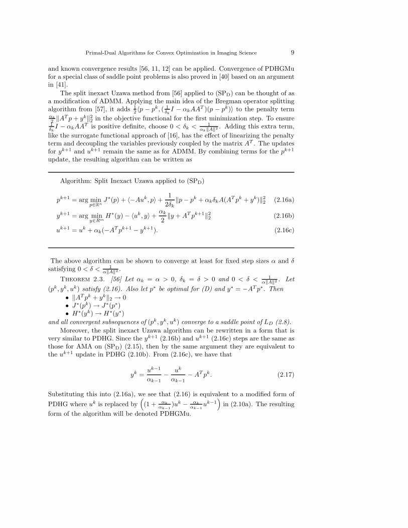
The split inexact Uzawa method from [56] applied to (SPD) can be thought of asa modification of ADMM. Applying the main idea of the Bregman operator splittingalgorithm from [57], it adds 1

2 〈p − pk, ( 1δk

I − αkAAT )(p − pk)〉 to the penalty termαk

2 ‖AT p + yk‖22 in the objective functional for the first minimization step. To ensure

1δk

I − αkAAT is positive definite, choose 0 < δk < 1αk‖A‖2 . Adding this extra term,

like the surrogate functional approach of [16], has the effect of linearizing the penaltyterm and decoupling the variables previously coupled by the matrix AT . The updatesfor yk+1 and uk+1 remain the same as for ADMM. By combining terms for the pk+1

update, the resulting algorithm can be written as

Algorithm: Split Inexact Uzawa applied to (SPD)


J∗(p) + 〈−Auk, p〉 +1

2δk

‖p − pk + αkδkA(AT pk + yk)‖22 (2.16a)

yk+1 = arg miny∈Rm

H∗(y) − 〈uk, y〉 +αk

2‖y + AT pk+1‖2

2 (2.16b)

uk+1 = uk + αk(−AT pk+1 − yk+1). (2.16c)

The above algorithm can be shown to converge at least for fixed step sizes α and δ

satisfying 0 < δ < 1α‖A‖2 .

Theorem 2.3. [56] Let αk = α > 0, δk = δ > 0 and 0 < δ < 1α‖A‖2 . Let

(pk, yk, uk) satisfy (2.16). Also let p∗ be optimal for (D) and y∗ = −AT p∗. Then

• ‖AT pk + yk‖2 → 0• J∗(pk) → J∗(p∗)• H∗(yk) → H∗(y∗)

and all convergent subsequences of (pk, yk, uk) converge to a saddle point of LD (2.8).

Moreover, the split inexact Uzawa algorithm can be rewritten in a form that isvery similar to PDHG. Since the yk+1 (2.16b) and uk+1 (2.16c) steps are the same asthose for AMA on (SPD) (2.15), then by the same argument they are equivalent tothe uk+1 update in PDHG (2.10b). From (2.16c), we have that

yk =uk−1

αk−1− uk

αk−1− AT pk. (2.17)

Substituting this into (2.16a), we see that (2.16) is equivalent to a modified form of

PDHG where uk is replaced by(

(1 + αk

αk−1)uk − αk

αk−1uk−1

)

in (2.10a). The resulting

form of the algorithm will be denoted PDHGMu.


Algorithm: PDHGMu


J∗(p) + 〈p,−A

(

(1 +αk

αk−1)uk − αk

αk−1uk−1

)

〉 +1

2δk

‖p− pk‖22

(2.18a)


H(u) + 〈AT pk+1, u〉 +1

2αk

‖u − uk‖22, (2.18b)

Note that from (2.17) and (2.18b), yk+1 ∈ ∂H(uk+1), which we could substituteinstead of (2.17) into (2.16a) to get an equivalent version of PDHGMu, whose updatesonly depend on the previous iteration instead of the previous two.

By the equivalence of PDHGMu and SIU on (SPD), Theorem 2.3 again appliesto the PDHGMu iterates with yk defined by (2.17). However, there is a strongerstatement for the convergence of PDHGMu in [11, 12].

Theorem 2.4. [11] Let αk = α > 0, δk = δ > 0 and 0 < δ < 1α‖A‖2 . Let (pk, uk)

satisfy (2.18). Then (uk, pk) converges to a saddle point of LPD (2.2).

Similarly, the corresponding split inexact Uzawa method applied to (SPP) is ob-tained by adding 1

2 〈u−uk, ( 1αk

I−δkAT A)(u−uk)〉 to the uk+1 step of ADMM applied

to (SPP). This leads to similar modification of PDHG denoted PDHGMp, where pk+1

is replaced by(

(1 +δk+1

δk)pk+1 − δk+1

δkpk

)

in (2.10b).

The modifications to uk and pk in the split inexact Uzawa methods are reminiscentof the predictor-corrector step in Chen and Teboulle’s predictor corrector proximalmethod (PCPM) [14]. Despite some close similarities, however, the algorithms arenot equivalent. The modified PDHG algorithms are more implicit than PCPM.

The connections between the algorithms discussed so far are diagrammed in Fig-ure 2.1. For simplicity, constant step sizes are assumed in the diagram. Double arrowsindicate equivalences between algorithms while single arrows show how to modify themto arrive at related methods.

3. PDHG for TV Deblurring . In this section we review from [58] the appli-cation of PDHG to the TV deblurring and denoising problems, but using the presentnotation. Both problems are of the form

minu∈Rm

‖u‖TV +λ

2‖Ku − f‖2

2, (3.1)

where ‖·‖TV denotes the discrete TV seminorm to be defined. If K is a linear blurringoperator, this corresponds to a TV regularized deblurring model. It also includes theTV denoising case when K = I. These applications are analyzed in [58], which alsomentions possible extensions such as to TV denoising with a constraint on the varianceof u and also l1 minimization.

3.1. Total Variation Discretization . We define a discretization of the totalvariation seminorm and in particular define a norm, ‖ · ‖E , and a matrix, D, suchthat ‖u‖TV = ‖Du‖E. Thus (3.1) is of the same form as the primal problem (P)with J(w) = ‖w‖E , A = D and H(u) = λ

2 ‖Ku − f‖22. The details are included for

completeness.


(P) minu FP (u)

FP (u) = J(Au) + H(u)

(D) maxp FD(p)

FD(p) = −J∗(p) − H∗(−AT p)

(PD) minu supp LPD(u, p)

LPD(u, p) = 〈p, Au〉 − J∗(p) + H(u)

(SPP) maxp infu,w LP (u, w, p)

LP (u, w, p) = J(w) + H(u) + 〈p, Au − w〉(SPD) maxu infp,y LD(p, y, u)

LD(p, y, u) = J∗(p) + H∗(y) + 〈u,−AT p − y〉

? ?

AMAon

(SPP)

-�PFBS

on(D)

PFBSon(P)

-�AMA

on(SPD)

PPPPPPPPPPq

��)+ 1

2α‖u − uk‖2

2 + 1

2δ‖p − pk‖2

2

��

��

��

��

��

AAAAAAAAAAAU

+ δ

2‖Au − w‖2

2 +α

2‖AT p + y‖2

2

Relaxed AMAon (SPP)

Relaxed AMAon (SPD)

@@@R@

@@I ��

��

ADMMon

(SPP)

-�

DouglasRachford

on(D)

DouglasRachford

on(P)

-�ADMM

on(SPD)

@@ ��

@@@R

��

+ 1

2〈u − uk, ( 1

αI − δAT A)(u − uk)〉 + 1

2〈p − pk, ( 1

δI − αAAT )(p − pk)〉

Primal-Dual Proximal Point on(PD)

=PDHG

��

��

@@

@@@R

pk+1 →

2pk+1 − pk

uk →

2uk − uk−1

SplitInexactUzawa

on (SPP)

-� PDHGMp PDHGMu -�

SplitInexactUzawa

on (SPD)

Legend: (P): Primal(D): Dual(PD): Primal-Dual(SPP): Split Primal(SPD): Split Dual

AMA: Alternating Minimization Algorithm (2.2.1)PFBS: Proximal Forward Backward Splitting (2.2.1)ADMM: Alternating Direction Method of Multipliers (2.2.2)PDHG: Primal Dual Hybrid Gradient (2.2)PDHGM: Modified PDHG (2.2.3)Bold: Well Understood Convergence Properties

Fig. 2.1. PDHG-Related Algorithm Framework


Define the discretized version of the TV seminorm by

‖u‖TV =

Mr∑

p=1

Mc∑

q=1

√

(D+1 up,q)2 + (D+

2 up,q)2 (3.2)

for u ∈ RMr×Mc . Here, D+

k represents a forward difference in the kth index andwe assume Neumann boundary conditions. It will be useful to instead work withvectorized u ∈ R

MrMc and to rewrite ‖u‖TV . The convention for vectorizing an Mr

by Mc matrix will be to associate the (p, q) element of the matrix with the (q−1)Mr+p

element of the vector. Consider a graph G(E ,V) defined by an Mr by Mc grid withV = {1, ..., MrMc} the set of m = MrMc nodes and E the set of e = 2MrMc−Mr−Mc

edges. Assume the nodes are indexed so that the node corresponding to element (p, q)is indexed by (q − 1)Mr + p. The edges, which will correspond to forward differences,can be indexed arbitrarily. Define D ∈ R

e×m to be the edge-node adjacency matrixfor this graph. So for a particular edge η ∈ E with endpoint indices i, j ∈ V and i < j,we have

Dη,ν =

−1 for ν = i,

1 for ν = j,

0 for ν 6= i, j.

(3.3)

The matrix D is a discretization of the gradient and −DT is the corresponding dis-cretization of the divergence.

Also define E ∈ Re×m such that

Eη,ν =

{

1 if Dη,ν = −1,

0 otherwise.(3.4)

The matrix E will be used to identify the edges used in each forward difference. Nowdefine a norm on R

e by

‖w‖E =

m∑

ν=1

(

√

ET (w2)

)

ν

. (3.5)

Note that in this context, the square root and w2 denote componentwise operations.Another way to interpret ‖w‖E is as the sum of the l2 norms of vectors wν , where

wν =

...we

...

for e such that Ee,ν = 1, ν = 1, ..., m. (3.6)

Typically, which is to say away from the boundary, wν is of the form wν =

[

weν1

weν2

]

,

where eν1 and eν

2 are the edges used in the forward difference at node ν. So in termsof wν , ‖w‖E =

∑mν=1 ‖wν‖2, and we take ‖wν‖2 = 0 in the case that wν is empty for

some ν. The discrete TV seminorm defined above (3.2) can be written in terms of‖ · ‖E as

‖u‖TV = ‖Du‖E.


Use of the matrix E is nonstandard, but also more general. For example, by re-defining D and adding edge weights, this notation can be easily extended to otherdiscretizations and even nonlocal TV.

By definition, the dual norm ‖ · ‖E∗ to ‖ · ‖E is

‖x‖E∗ = max‖y‖E≤1

〈x, y〉. (3.7)

This dual norm arises in the saddle point formulation of (3.1) that the PDHG algo-rithm for TV deblurring is based on. If xν is defined analogously to wν in (3.6), thenthe Cauchy Schwarz inequality can be used to show

‖x‖E∗ = maxν

‖xν‖2.

Altogether, ‖ · ‖E and ‖ · ‖E∗ are analogous to ‖ · ‖1 and ‖ · ‖∞ respectively and canbe expressed as

‖w‖E = ‖√

ET (w2)‖1 =

m∑

ν=1

‖wν‖2 and ‖x‖E∗ = ‖√

ET (x2)‖∞ = maxν

‖xν‖2.

3.2. Saddle Point Formulations. The saddle point formulation for PDHGapplied to TV minimization problems in [58] is based on the observation that

‖u‖TV = maxp∈X

〈p, Du〉, (3.8)

where

X = {p ∈ Re : ‖p‖E∗ ≤ 1} . (3.9)

The set X , which is the unit ball in the dual norm of ‖ · ‖E , can also be interpretedas a Cartesian product of unit balls in the l2 norm. For example, in order for Du

to be in X , the discretized gradient

[

up+1,q − up,q

up,q+1 − up,q

]

of u at each node (p, q) would

have to have Euclidean norm less than or equal to 1. The dual norm interpretationis another way to explain (3.8) since

max{p:‖p‖E∗≤1}

〈p, Du〉 = ‖Du‖E,

which equals ‖u‖TV by definition. Using duality to rewrite ‖u‖TV is common to manyprimal dual approaches for TV minimization including CGM [13], the second ordercone programming (SOCP) formulation used in [28] and the semismooth Newtonmethods in [30, 31, 17]. Here, analogous to the definition of (PD), it can be used toreformulate problem (3.1) as the min-max problem

minu∈Rm

maxp∈X

Φ(u, p) := 〈p, Du〉 +λ

2‖Ku − f‖2

2. (3.10)

3.3. Existence of Saddle Point . One way to ensure that there exists a saddlepoint (u∗, p∗) of the convex-concave function Φ is to restrict u and p to be in boundedsets. Existence then follows from ([43] 37.6). The dual variable p is already requiredto lie in the convex set X . Assume that

ker (D)⋂

ker (K) = {0}.


This is equivalent to assuming that ker (K) does not contain the vector of all ones,which is very reasonable for deblurring problems where K is an averaging operator.With this assumption, it follows that there exists c ∈ R such that the set

{

u : ‖Du‖E +λ

2‖Ku − f‖2

2 ≤ c

}

is nonempty and bounded. Thus we can restrict u to a bounded convex set.

3.4. Optimality Conditions. If (u∗, p∗) is a saddle point of Φ, it follows that

maxp∈X

〈p, Du∗〉 +λ

2‖Ku∗ − f‖2

2 = Φ(u∗, p∗) = minu∈Rm

〈p∗, Du〉 +λ

2‖Ku − f‖2

2,

from which we can deduce the optimality conditions

DT p∗ + λKT (Ku∗ − f) = 0 (3.11)

p∗E

√

ET (Du∗)2 = Du∗ (3.12)

p∗ ∈ X. (3.13)

The second optimality condition (3.12) with E defined by (3.4) can be understood asa discretization of p∗|∇u∗| = ∇u∗.

3.5. PDHG for Unconstrained TV Deblurring. In [58] it is shown howto interpret the PDHG algorithm applied to (3.1) as a primal-dual proximal pointmethod for solving (3.10) by iterating

pk+1 = arg maxp∈X

〈p, Duk〉 − 1

2λτk

‖p − pk‖22 (3.14a)


〈pk+1, Du〉 +λ

2‖Ku − f‖2

2 +λ(1 − θk)

2θk

‖u − uk‖22. (3.14b)

The index k denotes the current iteration. Also, τk and θk are the dual and primalstep sizes respectively. The parameters in terms of δk and αk from (2.10) are givenby

θk =λαk

1 + αkλτk =

δk

λ.

The above max and min problems can be explicitly solved, yielding

Algorithm: PDHG for TV Deblurring

pk+1 = ΠX

(

pk + τkλDuk)

(3.15a)

uk+1 =(

(1 − θk)I + θkKT K)−1

(

(1 − θk)uk + θk(KT f − 1

λDT pk+1)

)

. (3.15b)

Here, ΠX is the orthogonal projection onto X defined by

ΠX(q) = arg minp∈X

‖p − q‖22 =

q

E max(

√

ET (q2), 1) , (3.16)


where the division and max are understood in a componentwise sense. With qν definedanalogously to wν in (3.6), we could alternatively write (ΠX(q))η =

qη

max(‖qν‖2,1) ,

where ν is the node at which edge η is used in a forward difference. For example,ΠX(Du) can be thought of as a discretization of

{

∇u|∇u| if |∇u| > 1

∇u otherwise.

In the denoising case where K = I, the pk+1 update remains the same and the uk+1

simplifies to

uk+1 = (1 − θk)uk + θk(f − 1

λDT pk+1).

4. Interpretation of PDHG as Projected Averaged Gradient Methodfor TV Denoising . Even though we know of convergence results (Theorems 2.3and 2.4) for the modified PDHG algorithms PDHGMu (2.18) and PDHGMp, it wouldbe nice to show convergence of the original PDHG method (2.10) because PDHG stillhas some numerical advantages. Empirically, the stability requirements for the stepsize parameters are less restrictive for PDHG, so there is more freedom to tune theparameters to improve the rate of convergence. In this section, we restrict attentionto PDHG applied to TV denoising and prove a convergence result assuming certainconditions on the parameters.

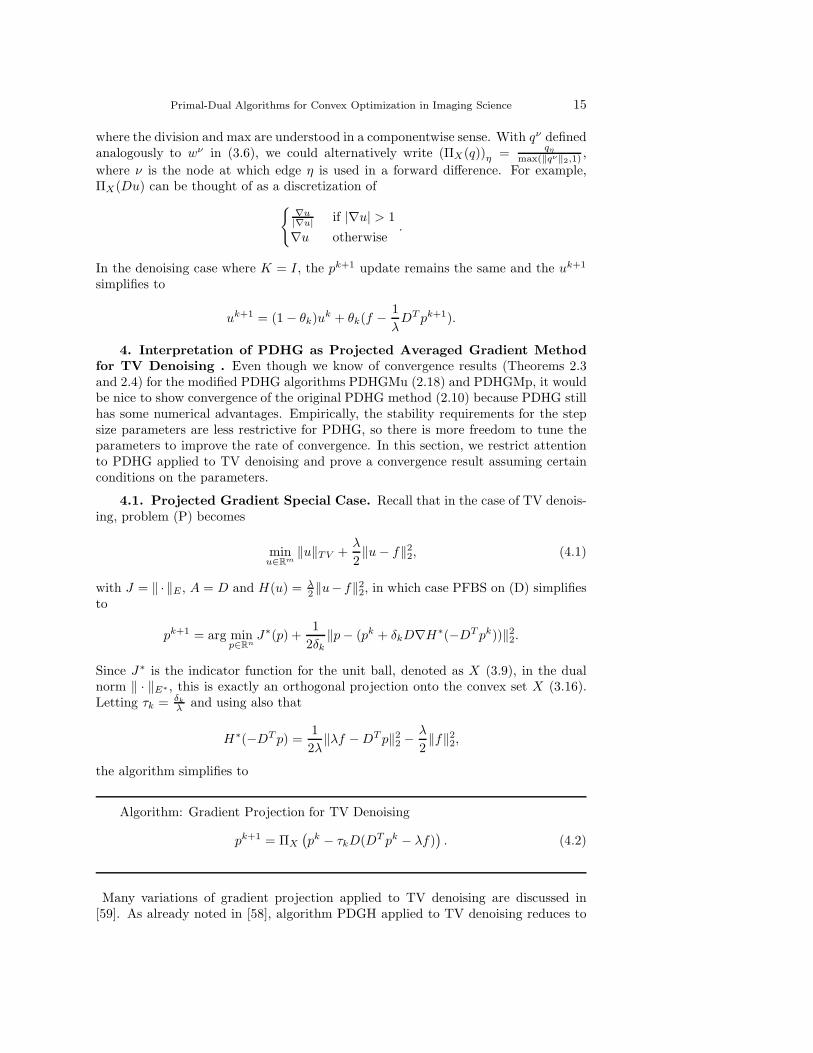
4.1. Projected Gradient Special Case. Recall that in the case of TV denois-ing, problem (P) becomes

minu∈Rm

‖u‖TV +λ

2‖u − f‖2

2, (4.1)

with J = ‖ · ‖E , A = D and H(u) = λ2 ‖u− f‖2

2, in which case PFBS on (D) simplifiesto


J∗(p) +1

2δk

‖p− (pk + δkD∇H∗(−DT pk))‖22.

Since J∗ is the indicator function for the unit ball, denoted as X (3.9), in the dualnorm ‖ · ‖E∗ , this is exactly an orthogonal projection onto the convex set X (3.16).Letting τk = δk

λand using also that

H∗(−DT p) =1

2λ‖λf − DT p‖2

2 −λ

2‖f‖2

2,

the algorithm simplifies to

Algorithm: Gradient Projection for TV Denoising

pk+1 = ΠX

(

pk − τkD(DT pk − λf))

. (4.2)

Many variations of gradient projection applied to TV denoising are discussed in[59]. As already noted in [58], algorithm PDGH applied to TV denoising reduces to


projected gradient descent when θk = 1. Equivalence to (3.15) in the θk = 1 casecan be seen by plugging uk = (f − 1

λDT pk) into the update for pk+1. This can be

interpreted as projected gradient descent applied to

minp∈X

G(p) :=1

2‖DT p − λf‖2

2, (4.3)

an equivalent form of the dual problem.Theorem 4.1. Fix p0 ∈ R

n. Let pk be defined by (4.2) with 0 < inf τk ≤ sup τk <14 , and define uk+1 = f − DT pk

λ. Then {pk} converges to a solution of (4.3), and {uk}

converges to a solution of (4.1).Proof. Since ∇G is Lipschitz continuous with Lipschitz constant ‖DDT ‖ and

uk+1 = ∇H∗(−DT pk) = f − DT pk

λ, then by Theorem 2.2 the result follows if 0 <

inf τk ≤ sup τk < 2‖DDT ‖

. The bound ‖DDT ‖ ≤ 8 follows from the Gersgorin circle

theorem.

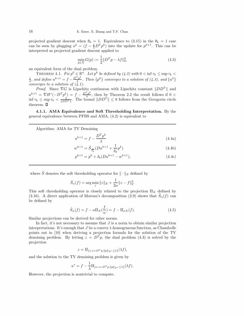
4.1.1. AMA Equivalence and Soft Thresholding Interpretation. By thegeneral equivalence between PFBS and AMA, (4.2) is equivalent to

Algorithm: AMA for TV Denoising

uk+1 = f − DT pk

λ(4.4a)

wk+1 = S 1δk

(Duk+1 +1

δk

pk) (4.4b)

pk+1 = pk + δk(Duk+1 − wk+1), (4.4c)

where S denotes the soft thresholding operator for ‖ · ‖E defined by

Sα(f) = argminz

‖z‖E +1

2α‖z − f‖2

2.

This soft thresholding operator is closely related to the projection ΠX defined by(3.16). A direct application of Moreau’s decomposition (2.9) shows that Sα(f) canbe defined by

Sα(f) = f − αΠX(f

α) = f − ΠαX(f). (4.5)

Similar projections can be derived for other norms.In fact, it’s not necessary to assume that J is a norm to obtain similar projection

interpretations. It’s enough that J be a convex 1-homogeneous function, as Chambollepoints out in [10] when deriving a projection formula for the solution of the TVdenoising problem. By letting z = DT p, the dual problem (4.3) is solved by theprojection

z = Π{z:z=DT p,‖p‖E∗≤1}(λf),

and the solution to the TV denoising problem is given by

u∗ = f − 1

λΠ{z:z=DT p,‖p‖E∗≤1}(λf).

However, the projection is nontrivial to compute.


4.2. Projected Averaged Gradient. In the θ 6= 1 case, still for TV denoising,the projected gradient descent interpretation of PDHG extends to an interpretation asa projected averaged gradient descent algorithm. Consider for simplicity parametersτ and θ that are independent of k. Then plugging uk+1 into the update for p yields

pk+1 = ΠX

(

pk − τdkθ

)

(4.6)

where

dkθ = θ

k∑

i=1

(1 − θ)k−i∇G(pi) + (1 − θ)k∇G(p0)

is a convex combination of gradients of G at the previous iterates pi. Note that dkθ is

not necessarily a descent direction.This kind of averaging of previous iterates suggests a connection to Nesterov’s

method [36]. Several recent papers study variants of his method and their applications.Weiss, Aubert and Blanc-Feraud in [51] apply a variant of Nesterov’s method [37] tosmoothed TV functionals. Beck and Teboulle in [1] and Becker, Bobin and Candesin [3] also study variants of Nesterov’s method that apply to l1 and TV minimizationproblems. Tseng gives a unified treatment of accelerated proximal gradient methodslike Nesterov’s in [50]. However, despite some tantalizing similarities to PDHG, itappears that none is equivalent.

In the following section, the connection to a projected average gradient methodon the dual is made for the more general case when the parameters are allowed todepend on k. Convergence results are presented for some special cases.

4.2.1. Convergence . For a minimizer p, the optimality condition for the dualproblem (4.3) is

p = ΠX(p − τ∇G(p)), ∀τ ≥ 0, (4.7)

or equivalently

〈∇G(p), p − p〉 ≥ 0, ∀p ∈ X.

In the following, we denote G = minp∈X G(p) and let X∗ denote the set of minimizers.As mentioned above, the PDHG algorithm (3.15) for TV denoising is related to aprojected gradient method on the dual variable p. When τ and θ are allowed todepend on k, the algorithm can be written as

pk+1 = ΠX

(

pk − τkdk)

(4.8)

where

dk =

k∑

i=0

sik∇G(pi), si

k = θi−1

k−1∏

j=i

(1 − θj).

Note that

k∑

i=0

sik = 1, si

k = (1 − θk−1)sik−1 ∀k ≥ 0, i ≤ k, and (4.9)

dk = (1 − θk−1)dk−1 + θk−1∇G(pk). (4.10)


As above, the direction dk is a linear (convex) combination of gradients of all previousiterates. We will show dk is an ǫ-gradient at pk. This means dk is an element of theǫ-differential (ǫ-subdifferential for nonsmooth functionals), ∂ǫG(p), of G at pk definedby

G(q) ≥ G(pk) + 〈dk, q − pk〉 − ǫ, ∀q ∈ X

When ǫ = 0 this is the definition of dk being a sub-gradient (in this case, the gradient)of G at pk.

For p and q, the Bregman distance based on G between p and q is defined as

D(p, q) = G(p) − G(q) − 〈∇G(q), p − q〉 ∀p, q ∈ X (4.11)

From (4.3), the Bregman distance (4.11) reduces to

D(p, q) =1

2‖DT (p − q)‖2

2 ≤ L

2‖p− q‖2,

where L is the Lipschitz constant of ∇G.Lemma 4.2. For any q ∈ X, we have

G(q) − G(pk) − 〈dk, q − pk〉 =

k∑

i=0

sik(D(q, pi) − D(pk, pi)).

Proof. For any q ∈ X ,

G(q) − G(pk) − 〈dk, q − pk〉 = G(q) − G(pk) − 〈k

∑

i=0

sik∇G(pi), q − pk〉

=

k∑

i=0

sikG(q) −

k∑

i=0

sikG(pi) −

k∑

i=0

sik〈∇G(pi), q − pi〉

+

k∑

i=0

sik(G(pi) − G(pk) − 〈∇G(pi), pi − pk〉)

=k

∑

i=0

sik(D(q, pi) − D(pk, pi))

Lemma 4.3. The direction dk is a ǫk-gradient of pk where ǫk =∑k

i=0 sikD(pk, pi).

Proof. By Lemma 4.2,

G(q) − G(pk) − 〈dk, q − pk〉 ≥ −k

∑

i=0

sikD(pk, pi) ∀q ∈ X.

By the definition of ǫ-gradient, we obtain that dk is a ǫk-gradient of G at pk, where

ǫk =

k∑

i=0

sikD(pk, pi).


Lemma 4.4. If θk → 1, then ǫk → 0.Proof. Let hk = G(pk) − G(pk−1) − 〈dk−1, pk − pk−1〉, then using the Lipschitz

continuity of ∇G and the boundedness of dk, we obtain

|hk| = |D(pk, pk−1)+〈(∇G(pk−1)−dk−1, pk−pk−1|〉| ≤ L

2‖pk−pk−1‖2

2+C1‖pk−pk−1‖2,

where L is the Lipschitz constant of ∇G, and C1 is some positive constant. Sinceǫk =

∑ki=0 si

kD(pk, pi), pk is bounded and∑

i=0 sik = 1, then ǫk is bounded for any k.

Meanwhile, by replacing q with pk and pk by pk−1 in Lemma 4.2, we obtainhk =

∑k−1i=0 si

k−1(D(pk, pi) − D(pk−1, pi)). From

sik = (1 − θk−1)s

ik−1, ∀ 1 ≤ i ≤ k − 1,

we get

ǫk = (1 − θk−1)

k−1∑

i=0

sik−1D(pk, pi)

= (1 − θk−1)ǫk−1 + (1 − θk−1)

k−1∑

i=0

sik−1(D(pk, pi) − D(pk−1, pi))

= (1 − θk−1)(ǫk−1 + hk).

By the boundness of hk and ǫk, we get immediately that if θk−1 → 1, then ǫk → 0.Since ǫk → 0, the convergence of pk follows directly from classical [47, 33] ǫ-

gradient methods. Possible choices of the step size τk are given in the followingtheorem:

Theorem 4.5. [47, 33][Convergence to the optimal set using divergent series τk]Let θk → 1 and let τk satisfy τk > 0, limk→∞ τk = 0 and

∑∞k=1 τk = ∞. Then the

sequence pk generated by (4.8) satisfies G(pk) → G and dist{pk, X∗} → 0.Since we require θk → 1, the algorithm is equivalent to projected gradient descent

in the limit. However, it is well known that a divergent step size for τk is slow andwe can expect a better convergence rate without letting τk go to 0. In the following,we prove a different convergence result that doesn’t require τk → 0 but still requiresθk → 1.

Lemma 4.6. For pk defined by (4.8), we have 〈dk, pk+1−pk〉 ≤ − 1τk‖pk+1−pk‖2

2.

Proof. Since pk+1 is the projection of pk − τkdk onto X , it follows that

〈pk − τkdk − pk+1, p − pk+1〉 ≤ 0, ∀p ∈ X.

Replacing p with pk, we thus get

〈dk, pk+1 − pk〉 ≤ − 1

τk

‖pk+1 − pk‖22. (4.12)

Lemma 4.7. Let pk be generated by the method (4.8), then

G(pk+1)−G(pk)−β2k

αk

‖pk−pk−1‖22 ≤ − (αk + βk)2

αk

‖pk−(αk

αk + βk

pk+1+βk

αk + βk

pk−1)‖22

where

αk =1

τkθk−1− L

2, βk =

1 − θk−1

2θk−1τk−1(4.13)


Proof. By using the Taylor expansion and the Lipschiz continuity of ∇G (ordirectly from the fact that G is quadratic function), we have

G(pk+1) − G(pk) ≤ 〈∇G(pk), pk+1 − pk〉 +L

2‖pk+1 − pk‖2

2,

Since by (4.10) ∇G(pk) = 1θk−1

(dk − (1 − θk−1)dk−1), using (4.12) we have

G(pk+1) − G(pk) ≤ 1

θk−1〈dk, pk+1 − pk〉 − 1 − θk−1

θk−1〈dk−1, pk+1 − pk〉 +

L

2‖pk+1 − pk‖2

2,

= (L

2− 1

τkθk−1)‖pk+1 − pk‖2

2 −1 − θk−1

θk−1〈dk−1, pk+1 − pk〉.

On the other hand, since pk is the projection of pk−1 − τk−1dk−1, we get

〈pk−1 − τk−1dk−1 − pk, p − pk〉 ≤ 0, ∀p ∈ X.

Replacing p with pk+1, we thus get

〈dk−1, pk+1 − pk〉 ≥ 1

τk−1〈pk−1 − pk, pk+1 − pk〉.

This yields

G(pk+1) − G(pk) ≤ −αk‖pk+1 − pk‖2 − 2βk〈pk−1 − pk, pk+1 − pk〉

= − (αk + βk)2

αk

‖pk − (αk

αk + βk

pk+1 +βk

αk + βk

pk−1)‖2 +β2

k

αk

‖pk − pk−1‖2.

where αk and βk are defined as (4.13).

Theorem 4.8. If αk and βk defined as (4.13) such that αk > 0, βk ≥ 0 and

∞∑

k=0

(αk + βk)2

αk

= ∞,

∞∑

k=0

β2k

αk

< ∞, limk→∞

βk

αk

= 0. (4.14)

then every limit point pair (p∞, d∞) of a subsequence of (pk, dk) is such that p∞ is aminimizer of (4.3) and d∞ = ∇G(p∞).

Proof. The proof is adapted from [5](Proposition 2.3.1,2.3.2) and Lemma 4.7.Since pk and dk are bounded, the subsequence (pk, dk) has a convergent subsequence.Let (p∞, d∞) be a limit point of the pair (pk, dk), and let (pkm , dkm) be a subsequencethat converges to (p∞, d∞). For km > n0, lemma 4.7 implies that

G(pkm)−G(pn0) ≤ −km∑

k=n0

(αk + βk)2

αk

‖pk−(αk

αk + βk

pk+1+βk

αk + βk

pk−1)‖22+

km∑

k=n0

β2k

αk

‖pk−1−pk‖22.

By the boundness of the constraint set X , the conditions (4.14) for αk and βk andthe fact that G(p) is bounded from below, we conclude that

‖pk − (αk

αk + βk

pk+1 +βk

αk + βk

pk−1)‖2 → 0.


Given ǫ > 0, we can choose m large enough such that ‖pkm − p∞‖2 ≤ ǫ3 , ‖pk −

( αk

αk+βkpk+1 + βk

αk+βkpk−1)‖2 ≤ ǫ

3 for all k ≥ km, andβkm

αkm+βkm‖(pkm−1 − p∞)‖2 ≤ ǫ

3 .

This third requirement is possible because limk→∞βk

αk= 0. Then

‖(pkm − p∞) − αkm

αkm+ βkm

(pkm+1 − p∞) − βkm

αkm+ βkm

(pkm−1 − p∞)‖2 ≤ ǫ

3

implies

‖ αkm

αkm+ βkm

(pkm+1 − p∞) +βkm

αkm+ βkm

(pkm−1 − p∞)‖2 ≤ 2

3ǫ.

Sinceβkm

αkm+βkm‖(pkm−1 − p∞)‖2 ≤ ǫ

3 , we have

‖pkm+1 − p∞‖2 ≤ αkm+ βkm

αkm

ǫ.

Note that km + 1 is not necessarily an index for the subsequence {pkm}. Sincelimk

αk+βk

αk= 1, then we have ‖pkm+1 − p∞‖2 → 0 when m → ∞. According (4.8),

the limit point p∞, d∞ is therefore such that

p∞ = ΠX(p∞ − τd∞) (4.15)

for τ > 0.It remains to show that the corresponding subsequence dkm = (1−θkm−1)d

km−1+θkm−1∇G(pkm) converges to ∇G(p∞). By the same technique, and the fact thatθk → 1, we can get ‖∇G(pkm)− d∞‖ ≤ ǫ. Thus ∇G(pkm) → d∞. On the other hand,∇G(pkm) → ∇G(p∞). Thus d∞ = ∇G(p∞). Combining with (4.15) and the optimalcondition (4.7), we conclude that p∞ is a minimizer.

In summary, the overall conditions on θk and τk are:• θk → 1, τk > 0,• 0 < τkθk < 2

L,

• ∑∞k=0

(αk+βk)2

αk= ∞,

• limk→∞βk

αk= 0,

• ∑∞k=0

β2k

αk< ∞,

where

αk =1

τkθk−1− L

2, βk =

1 − θk−1

2θk−1τk−1. (4.16)

Finally, we have θk → 1, and for τk the classical condition for the projected gra-dient descent algorithm, (0 < τk < 2

L), and divergent stepsize, (limk τk → 0,

∑

k τk →∞), are special cases of the above conditions. The algorithm converges empiricallyfor a much wider range of parameters. For example, convergence with 0 < θk ≤ c < 1and even θk → 0 is numerically demonstrated in [58], but a theoretical proof is stillan open problem.

5. Extensions to Constrained Minimization . The extension of PDHG toconstrained minimization problems is discussed in [58] and applied for example toTV denoising with a constraint of the form ‖u − f‖2 ≤ mσ2 with σ2 an estimateof the variance of the Gaussian noise. Such extensions work equally well with themodified PGHD algorithms. In the context of our general primal problem (P), if u isconstrained to be in a convex set S, then this still fits in the framework of (P) sincethe indicator function for S can be incorporated into the definition of H(u).


5.1. General Convex Constraint. Consider the case when H(u) is exactlythe indicator function gS(u) for a convex set S ⊂ R

m, which would mean

H(u) = gS(u) :=

{

0 if u ∈ S

∞ otherwise.

Applying PDHG or the modified versions results in a primal step that can be inter-preted as an orthogonal projection onto S. For example, when applying PDHGMu,the pk+1 step (2.18a) remains the same and the uk+1 step (2.18b) becomes

uk+1 = ΠS

(

uk − αkAT pk+1)

.

For this algorithm to be practical, the projection ΠS must be straightforward tocompute. Suppose the constraint on u is of the form ‖Ku− f‖2 ≤ ǫ for some matrixK and ǫ > 0. Then

ΠS(z) = (I − K†K)z + K†

{

Kz if ‖Kz − f‖2 ≤ ǫ

f + r(

Kz−KK†f‖Kz−KK†f‖2

)

otherwise,

where

r =√

ǫ2 − ‖(I − KK†)f‖22

and K† denotes the pseudoinverse of K. Note that (I −K†K) represents the orthog-onal projection onto ker (K). A special case where this projection is easily computedis when KKT = I and K† = KT . In this case, the projection onto S simplifies to

ΠS(z) = (I − KT K)z + KT

{

Kz if ‖Kz − f‖2 ≤ ǫ

f + ǫ(

Kz−f‖Kz−f‖2

)

otherwise.

5.2. Constrained TV deblurring. In the notation of problem (P), the un-constrained TV deblurring problem (3.1) corresponds to J = ‖ · ‖E, A = D andH(u) = λ

2 ‖Ku − f‖22. A constrained version of this problem,

min‖Ku−f‖2≤ǫ

‖u‖TV , (5.1)

can be rewritten as

minu

‖Du‖E + gT (Ku),

where gT is the indicator function for T = {z : ‖z − f‖2 ≤ ǫ} defined by

gT (z) =

{

0 ‖z − f‖2 ≤ ǫ

∞ otherwise.(5.2)

With the aim of eventually ending up with an explicit algorithm for this problem, weuse some operator splitting ideas, letting

H(u) = 0 and J(Au) = J1(Du) + J2(Ku),

where A =

[

D

K

]

, J1(w) = ‖w‖E and J2(z) = gT (z). Letting p =

[

p1

p2

]

, it follows that

J∗(p) = J∗1 (p1)+J∗

2 (p2). Applying PDHG (2.10) with the uk+1 step written first, weobtain


Algorithm: PDHG for Constrained TV Deblurring

uk+1 = uk − αk(DT pk1 + KT pk

2) (5.3a)

pk+11 = ΠX

(

pk1 + δkDuk+1

)

(5.3b)

pk+12 = pk

2 + δkKuk+1 − δkΠT

(

pk2

δk

+ Kuk+1

)

, (5.3c)

where ΠT is defined by

ΠT (z) = f +z − f

max(

‖z−f‖2

ǫ, 1

) . (5.4)

In the constant step size case, to get the PDHGMp version of this algorithm, we wouldreplace DT pk

1 + KT pk2 with DT (2pk

1 − pk−11 ) + KT (2pk

2 − pk−12 ).

5.3. Constrained l1-Minimization. Sparse approximation problems that seekto find a sparse solution satisfying some data constraints sometimes use the type ofconstraint described in the previous section [9]. A simple example of such a problemis

minu

‖u‖1 such that ‖Ku − f‖2 ≤ ǫ, (5.5)

where u is what we expect to be sparse, K = RΓΨT , R is a row selector, Γ isorthogonal and Ψ is a tight frame with ΨT Ψ = I. RΓ can be thought of as selectingsome coefficients in an orthonormal basis. We will compare two different applicationsof PDHGMu, one that stays on the constraint set and one that doesn’t.

Letting J = ‖ · ‖1, A = I, S = {u : ‖Ku− f‖2 ≤ ǫ} and H(u) equal the indicatorfunction gS(u) for S, application of PDHGMu yields a method such that uk satisfiesthe constraint at each iteration.

Algorithm: PDHGMu for Constrained l1-Minimization: (stays in constraint set)

pk+1 = Π{p:‖p‖∞≤1}

(

pk + δk

(

(1 +αk

αk−1)uk − αk

αk−1uk−1

))

(5.6a)

uk+1 = ΠS

(

uk − αkpk+1)

, (5.6b)

where

Π{p:‖p‖∞≤1}(p) =p

max(|p|, 1)

and

ΠS(u) = (I − KT K)u + KT

f +Ku − f

max(

‖Ku−f‖2

ǫ, 1

)

.


As before, Theorem 2.4 applies when αk = α > 0, δk = δ > 0 and δ < 1α. Also, since

A = I, the case when δ = 1α

is exactly ADMM applied to (SPD), which is equivalentto Douglas Rachford splitting on (P).

In general, ΠS may be difficult to compute. It is possible to apply PDHGMu to(5.5) in a way that simplifies this projection but no longer stays in the constraint setat each iteration. The strategy is essentially to reverse the roles of J and H in theprevious example, letting J(u) = gT (Ku) and H(u) = ‖u‖1 with gT defined by (5.2).The resulting algorithm is

Algorithm: PDHGMu for Constrained l1-Min.: (doesn’t stay in constraint set)

vk+1 = pk + δkK

(

(1 +αk

αk−1)uk − αk

αk−1uk−1

)

(5.7a)

pk+1 = vk+1 − δkΠT

(

vk+1

δk

)

(5.7b)

wk+1 = uk − αkKT pk+1 (5.7c)

uk+1 = wk+1 − αkΠ{p:‖p‖∞≤1}

(

wk+1

αk

)

. (5.7d)

Here, vk+1 and wk+1 are just place holders and ΠT is defined by (5.4).This variant of PDHGMu is still an application of the split inexact Uzawa method

(2.16). Also, since ‖K‖ ≤ 1, the conditions for convergence are the same as for (5.6).Moreover, since KKT = I, if δ = 1

α, then this method can again be interpreted as

ADMM applied to the split dual problem.Note that ΠT is much simpler to compute than ΠS . The benefit of simplifying

the projection step is important for problems where K† is not practical to deal withnumerically.

6. Numerical Experiments . We perform three numerical experiments toshow the modified and unmodified PDHG algorithms have similar performance andapplications. The first is a comparison between PDHG, PDHGMu and ADMM ap-plied to TV denoising. The second compares the application of PDHG and PDHGMpto a constrained TV deblurring problem. The third experiment applies PDHGMu intwo different ways to a constrained l1 minimization problem.

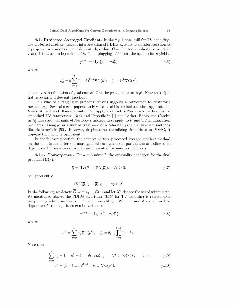
6.1. PDHGM, PDHG and ADMM for TV denoising. Here, we closelyfollow the numerical example presented in Table 4 of [58], which compared PDHG toChambolle’s method [10] and CGM [13] for TV denoising. We use the same 256×256cameraman image with intensities in [0, 255]. The image is corrupted with zero meanwhite Gaussian noise having standard deviation 20. We also use the same parameterλ = .053. Both adaptive and fixed stepsize strategies are compared. In all examples,we initialize u0 = f and p0 = 0. Figure 6.1 shows the clean and noisy images alongwith a benchmark solution for the denoised image.

Recall the PDHG algorithm for the TV denoising problem (4.1) is given by (3.15)with K = I. The adaptive strategy used for PDHG is the same one proposed in [58]where

τk = .2 + .008k θk =.5 − 5

15+k

τk

. (6.1)


Fig. 6.1. Original, noisy and benchmark denoised cameraman images

These can be related to the step sizes δk and αk in (2.10) by

δk = λτk αk =θk

λ(1 − θk).

These time steps don’t satisfy the requirements of Theorem 4.8, which requires θk → 1.However, we find that the adaptive PDHG strategy (6.1), for which θk → 0, is muchbetter numerically for TV denoising.

When applying the PDHGMu algorithm to TV denoising, the stability require-ment means using the same adaptive time steps of (6.1) can be unstable. Instead, theadaptive strategy we use for PDHGMu is

αk =1

λ(1 + .5k)δk =

1

8.01αk

(6.2)

Unfortunately, no adaptive strategy for PDHGMu can satisfy the requirements ofTheorem 2.3, which assumes fixed time steps. However, the rate of convergence ofthe adaptive PDHGMu strategy for TV denoising is empirically better than the fixedparameter strategies.

We also perform some experiments with fixed α and δ. A comparison is made togradient projection (4.2). We also compare to FISTA [1] applied to the dual of theTV denoising problem (4.3). As discussed in [2], where this application is referredto as FGP, it can be thought of as an acceleration of gradient projection. Muchlike the modification to PDHG, it replaces pk in (4.2) with a combination of the

previous iterates, namely pk+ tk−1tk+1

(pk−pk−1), where tk+1 =1+

√1+4t2

k

2 . An additional

comparison is made to ADMM as applied to (SPP). This algorithm alternates softthresholding, solving a Poisson equation and updating the Lagrange multiplier. Thisis equivalent to the split Bregman algorithm [29], which was compared to PDHGelsewhere in [58]. However, by working with the ADMM form of the algorithm, it’seasier to use the duality gap as a stopping condition since u and p have the sameinterpretations in both algorithms. As in [58] we use the relative duality gap R forthe stopping condition defined by

R(u, p) =FP (u) − FD(p)

FD(p)=

(

‖u‖TV + λ2 ‖u − f‖2

2

)

−(

λ2 ‖f‖2

2 − 12λ‖DT p − λf‖2

2

)

λ2 ‖f‖2

2 − 12λ‖DT p − λf‖2

2

,

which is the duality gap divided by the dual functional. The duality gap is definedto be the difference between the primal and dual functionals. This quantity is always


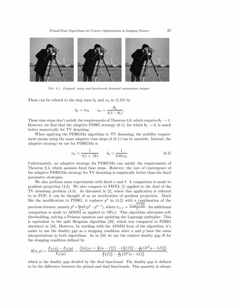
Algorithm tol = 10−2 tol = 10−4 tol = 10−6

PDHG (adaptive) 14 70 310PDHGMu (adaptive) 19 92 365

PDHG α = 5, δ = .025 31 404 8209PDHG α = 1, δ = .125 51 173 1732PDHG α = .2, δ = .624 167 383 899PDHGMu α = 5, δ = .025 21 394 8041PDHGMu α = 1, δ = .125 38 123 1768PDHGMu α = .2, δ = .624 162 355 627

PDHG α = 5, δ = .1 22 108 2121PDHG α = 1, δ = .5 39 123 430PDHG α = .2, δ = 2.5 164 363 742PDHGMu α = 5, δ = .1 unstablePDHGMu α = 1, δ = .5 unstablePDHGMu α = .2, δ = 2.5 unstable

Proj. Grad. δ = .0132 46 721 14996FGP δ = .0066 24 179 1264

ADMM δ = .025 17 388 7951ADMM δ = .125 22 100 1804ADMM δ = .624 97 270 569

Table 6.1

Iterations Required for TV Denoising

nonnegative, and is zero if and only if (u, p) is a saddle point of (3.10) with K = I.Table 6.1 shows the number of iterations required for the relative duality gap to fallbelow tolerances of 10−2, 10−4 and 10−6. Note that the complexity of the PDHGand PDHGMu iterations scale like O(m) whereas the ADMM iterations scale likeO(m log m). Results for PDHGMp were identical to those for PDHGMu and aretherefore not included in the table. All the examples are for the same 256 × 256cameraman image. As the problem size increases, more iterations would be requiredfor all the tabulated methods.

From Table 6.1, we see that PDHG and PDHGMu both benefit from adaptivestepsize schemes. The adaptive versions of these algorithms are compared in Figure6.3(a), which plots the relative l2 error to the benchmark solution versus number ofiterations. PDHG with the adaptive stepsizes outperforms all the other numericalexperiments, but for identical fixed parameters, PDHGMu performed slightly betterthan PDHG. However, for fixed α the stability requirement, δ < 1

α‖D‖2 for PDHGMu

places an upper bound on δ which is empirically about four times less than for PDHG.Table 6.1 shows that for fixed α, PDHG with larger δ outperforms PDHGMu. Thestability restriction for PDHGMu is also why the same adaptive time stepping schemeused for PDHG could not be used for PDHGMu. We also note that fixed parameterversions of PDHG and PDHGMu are competitive with FGP.

Table 6.1 also demonstrates that larger α is more effective when the relative


duality gap is large, and smaller α is better when this duality gap is small. SincePDHG for large α is similar to projected gradient descent, roughly speaking thismeans the adaptive PDHG algorithm starts out closer to PFBS on (D), but graduallybecomes more like PFBS on (P).

All the methods in Table 6.1 are at best linearly convergent, so superlinearlyconvergent methods like CGM and semismooth Newton will eventually outperformthem when high accuracy is desired.

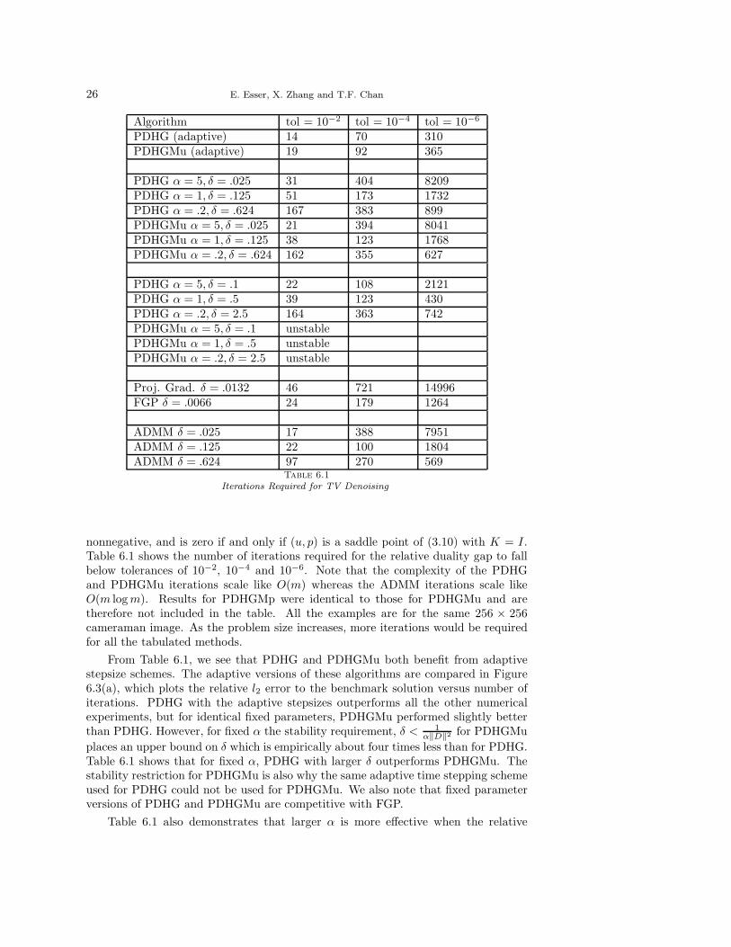
6.2. PDHGMp for Constrained TV Deblurring. PDHGMp and PDHGalso perform similarly for constrained TV deblurring (5.1). For this example we usethe same cameraman image from the previous section and let K be a convolutionoperator corresponding to a normalized Gaussian blur with a standard deviation of 3in a 17 by 17 window. Letting h denote the clean image, the given data f is takento be f = Kh + η, where η is zero mean Gaussian noise with standard deviation 1.We thus set ǫ = 256. For the numerical experiments we used the fixed parameterversions of PDHG and PDHGMp with α = .33 and δ = .33. The images h, f

and the recovered image from 300 iterations of PDHGMp are shown in Figure 6.2.Figure 6.3(b) compares the relative l2 error to the benchmark solution as a function

Fig. 6.2. Original, blurry/noisy and image recovered from 300 PDHGMp iterations

of number of iterations for PDHG and PDHGMp. Empirically, with the same fixedparameters, the performance of these two algorithms is nearly identical, and the curvesare indistinguishable in Figure 6.3(b). Although many iterations are required for ahigh accuracy solution, Figure 6.2 shows the result can be visually satisfactory afterjust a few hundred iterations.

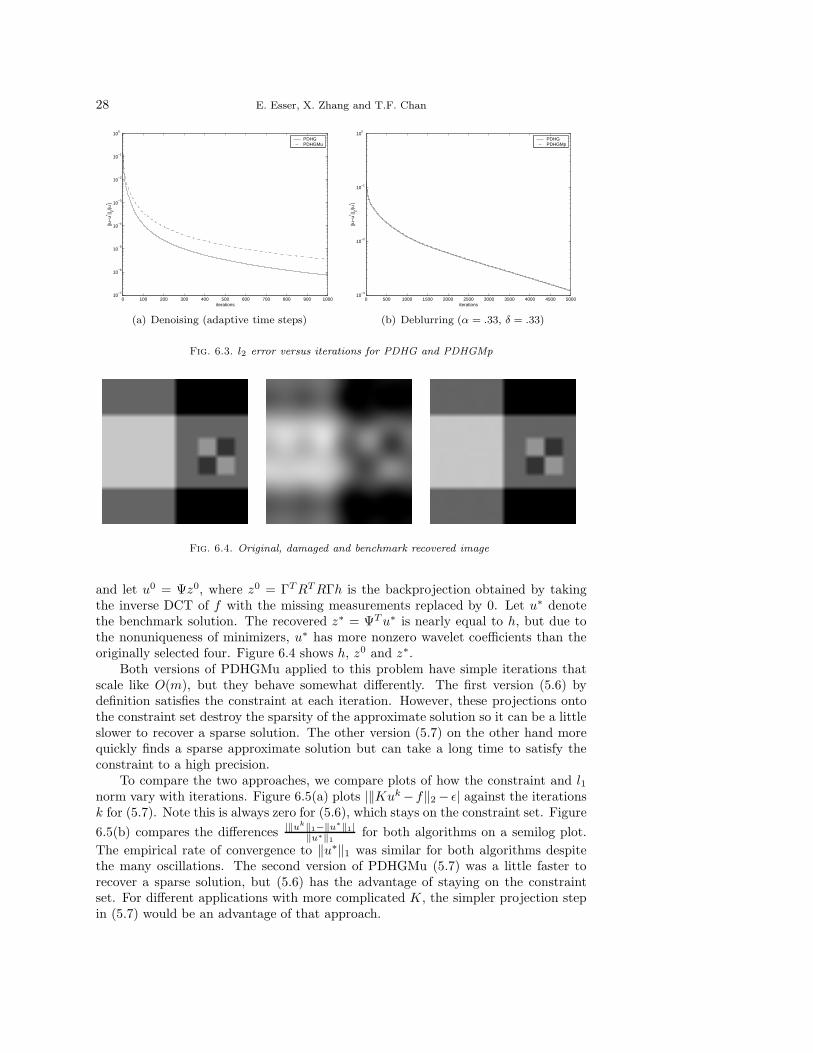
6.3. PDHGMu for Constrained l1 Minimization. Here we compare twoapplications of PDHGMu, (5.6) and (5.7), applied to (5.5) with ǫ = .01. Let K =RΓΨT , where R is a row selector, Γ is an orthogonal 2D discrete cosine transformand Ψ is a redundant translation invariant 2D Haar wavelet transform normalized sothat ΨT Ψ = I. It follows that KKT = I and K† = KT . For a simple example, leth be a 32 × 32 image, shown in Figure 6.4, that is a linear combination of just fourHaar wavelets. Let R select 64 of the lowest frequency DCT measurements and definef = RΓh. The constrained l1 minimization model aims to recover a sparse signalin the wavelet domain that is consistent with these partial DCT measurements [8].We’ve kept the example simple so as to focus on the two possible ways to handle theconstraint using PDHGMu.

For the numerical experiments, we let α = .99 and δ = .99. We also scale ‖u‖1

by µ = 10 to accelerate the rate of convergence. For the initialization, let p0 = 0


0 100 200 300 400 500 600 700 800 900 100010

−7

10−6

10−5

10−4

10−3

10−2

10−1

100

iterations

||u−

u* || 2/|u* |

PDHG PDHGMu

(a) Denoising (adaptive time steps)

0 500 1000 1500 2000 2500 3000 3500 4000 4500 500010

−3

10−2

10−1

100

iterations

||u−

u* || 2/|u* |

PDHG PDHGMp

(b) Deblurring (α = .33, δ = .33)

Fig. 6.3. l2 error versus iterations for PDHG and PDHGMp

Fig. 6.4. Original, damaged and benchmark recovered image

and let u0 = Ψz0, where z0 = ΓT RT RΓh is the backprojection obtained by takingthe inverse DCT of f with the missing measurements replaced by 0. Let u∗ denotethe benchmark solution. The recovered z∗ = ΨT u∗ is nearly equal to h, but due tothe nonuniqueness of minimizers, u∗ has more nonzero wavelet coefficients than theoriginally selected four. Figure 6.4 shows h, z0 and z∗.

Both versions of PDHGMu applied to this problem have simple iterations thatscale like O(m), but they behave somewhat differently. The first version (5.6) bydefinition satisfies the constraint at each iteration. However, these projections ontothe constraint set destroy the sparsity of the approximate solution so it can be a littleslower to recover a sparse solution. The other version (5.7) on the other hand morequickly finds a sparse approximate solution but can take a long time to satisfy theconstraint to a high precision.

To compare the two approaches, we compare plots of how the constraint and l1norm vary with iterations. Figure 6.5(a) plots |‖Kuk − f‖2 − ǫ| against the iterationsk for (5.7). Note this is always zero for (5.6), which stays on the constraint set. Figure

6.5(b) compares the differences |‖uk‖1−‖u∗‖1|‖u∗‖1

for both algorithms on a semilog plot.

The empirical rate of convergence to ‖u∗‖1 was similar for both algorithms despitethe many oscillations. The second version of PDHGMu (5.7) was a little faster torecover a sparse solution, but (5.6) has the advantage of staying on the constraintset. For different applications with more complicated K, the simpler projection stepin (5.7) would be an advantage of that approach.


0 500 1000 1500 2000 2500 3000 3500 4000 4500 500010

−2

10−1

100

101

102

103

104

iterations

| ||K

u−f||

2−ε

|

(a) Constraint versus iterations for PDHGMuversion (5.6) (α = .99, δ = .99)

0 500 1000 1500 2000 2500 3000 3500 4000 4500 500010

−10

10−9

10−8

10−7

10−6

10−5

10−4

10−3

10−2

10−1

100

| |u|

1 − |u

* | 1 |/|u

* | 1

iterations

PDHGMu: stays in constraint set PDHGMu: doesn’t stay in constraint set

(b) l1 Norm Comparison (α = .99, δ = .99)

Fig. 6.5. Comparison of two applications of PDHGMu to constrained l1 minimization

Acknowledgements. This work was supported by ONR N00014-03-1-0071, NSFDMS-0610079, NSF CCF-0528583 and NSF DMS-0312222. Thanks to Paul Tseng forpointing out some key references and for helpful discussions about PDHG and theMoreau decomposition. Thanks also to the anonymous referees, whose commentshave significantly improved the quality of this paper.

REFERENCES

[1] A. Beck, and M. Teboulle, A Fast Iterative Shrinkage-Thresholding Algorithm for LinearInverse Problems, SIAM J. Imaging Sciences, Vol. 2, 2009, pp. 183–202.

[2] A. Beck, and M. Teboulle, Fast Gradient-Based Algorithms for Con-strained Total Variation Image Denoising and Deblurring Problems,http://www.math.tau.ac.il/ teboulle/papers/tlv.pdf, 2009.

[3] S. Becker, J. Bobin, and E. J. Candes, NESTA: A Fast and Accurate First-Order Methodfor Sparse Recovery, http://www.acm.caltech.edu/ emmanuel/papers/NESTA.pdf, 2009.

[4] D. Bertsekas, Constrained Optimization and Lagrange Multiplier Methods, Athena Scientific,1996.

[5] D. Bertsekas, Nonlinear Programming, Athena Scientific, Second Edition, 1999.[6] D. Bertsekas, and J. Tsitsiklis, Parallel and Distributed Computation, Prentice Hall, 1989.[7] S. Boyd, and L. Vandenberghe, Convex Analysis, Cambridge University Press, 2006.[8] E. Candes, and J. Romberg, Practical Signal Recovery from Random Projections, IEEE

Trans. Signal Processing, 2005.[9] E. Candes, J. Romberg, and T. Tao, Stable signal recovery from incomplete and inaccurate

measurements, Comm. Pure Appl. Math., 59, 2005, pp. 1207-1223.[10] A. Chambolle, An Algorithm for Total Variation Minimization and Applications, J. Math.

Imaging Vision, Vol. 20, 2004, pp. 89-97.[11] A. Chambolle, V. Caselles, M. Novaga, D. Cremers and T. Pock, An

introduction to Total Variation for Image Analysis, http://hal.archives-ouvertes.fr/docs/00/43/75/81/PDF/preprint.pdf, 2009.

[12] A. Chambolle and T. Pock, A First-Order Primal-Dual Algorithm forConvex Problems with Applications to Imaging, http://hal.archives-ouvertes.fr/docs/00/49/08/26/PDF/pd alg final.pdf, 2010.

[13] T. F. Chan, G. H. Golub, and P. Mulet, A nonlinear primal dual method for total variationbased image restoration, SIAM J. Sci. Comput., 20, 1999.

[14] G. Chen, and M. Teboulle, A Proximal-Based Decomposition Method for Convex Minimiza-tion Problems, Math. Program. Vol., 64, 1994, pp. 81-101.

[15] P. Combettes, and W. Wajs, Signal Recovery by Proximal Forward-Backward Splitting, Mul-tiscale Model. Simul., 2006.

[16] I. Daubechies, M. Defrise, and C. De Mol, An Iterative Threshilding Algorithm for Linear


Inverse Problems with a Sparsity Constraint, Comm. Pure and Appl. Math, Vol. 57, 2004.[17] Y. Dong, M. Hintermuller and M. Neri, An Efficient Primal-Dual Method for L1TV Image

Restoration, SIAM J. Imag. Sci. Vol. 2, No. 4, 2009, pp. 1168–1189.[18] J. Douglas, and H. H. Rachford, On the Numerical Solution of Heat Conduction Problems

in Two and Three Space Variables, Trans. Amer. Math. Soc. 82, 1956, pp. 421-439.[19] J. Eckstein, Splitting Methods for Monotone Operators with Applications to Parallel Opti-

mization, Ph. D. Thesis, Massachusetts Institute of Technology, Dept. of Civil Engineering,http://hdl.handle.net/1721.1/14356, 1989.

[20] J. Eckstein, and D. Bertsekas, On the Douglas-Rachford splitting method and the proximalpoint algorithm for maximal monotone operators, Math. Program. 55, 1992, pp. 293-318.

[21] I. Ekeland, and R. Temam, Convex Analysis and Variational Problems, SIAM, Classics inApplied Mathematics, 28, 1999.

[22] A. Elmoataz, O. Lezoray, and S. Bougleux, Nonlocal Discrete Regularization on WeightedGraphs: A framework for Image and Manifold Processing, IEEE, Vol. 17, No. 7, July 2008.

[23] E. Esser, Applications of Lagrangian-Based Alternating Direction Methods and Connectionsto Split Bregman, UCLA CAM Report [09-31], April 2009.

[24] D. Gabay, Methodes numeriques pour l’optimisation non-lineaire, These de Doctorat d’Etatet Sciences Mathematiques, Universite Pierre et Marie Curie, 1979.

[25] D. Gabay, and B. Mercier, A dual algorithm for the solution of nonlinear variational prob-lems via finite-element approximations, Comp. Math. Appl., 2 1976, pp. 17-40.

[26] R. Glowinski, and P. Le Tallec, Augmented Lagrangian and Operator-splitting Methods inNonlinear Mechanics, SIAM 1989.

[27] R. Glowinski, and A. Marrocco, Sur lapproximation par elements finis dordre un, et laresolution par penalisation-dualite dune classe de problemes de Dirichlet nonlineaires, Rev.Francaise dAut. Inf. Rech. Oper., R-2, 1975, pp. 41-76.

[28] D. Goldfarb, and W. Yin, Second-order Cone Programming Methods for Total Variation-Based Image Restoration, SIAM J. Sci. Comput. Vol. 27, No. 2, 2005, pp. 622-645.

[29] T. Goldstein and S. Osher, The Split Bregman Algorithm for L1 Regularized Problems,SIAM J. Imag. Sci. Vol. 2, No. 2, 2009, pp. 323-343.

[30] M. Hintermuller and K. Kunisch, Total Bounded Variation Regularization as BilaterallyConstrained Optimization Problem, SIAM J. Appl. Math., Vol. 64, 2004, pp. 311-1333.

[31] M. Hintermuller and G. Stadler, An Infeasible Primal-Dual Algorithm for Total BoundedVariation-Based Inf-Convolution-Type Image Restoration, SIAM J. Sci. Comput. Vol. 28,No. 1, 2006, pp. 1-23.

[32] R. A. Horn, and C. R. Johnson, Matrix Analysis, Cambridge University Press, 1985.[33] F. Larsson, M. Patriksson, and A.-B. Stromberg, On the convergence of conditional ǫ-

subgradient methods for convex programs and convex-concave saddle-point problems, Eu-ropean J. Oper. Res., Vol. 151, No. 3, 2003, pp. 461-473.

[34] P. L. Lions, and B. Mercier, Algorithms for the Sum of Two Nonlinear Operators, SIAM J.Numer. Anal., Vol. 16, No. 6, Dec., 1979, pp. 964-979.

[35] J. J. Moreau, Proximite et dualite dans un espace hilbertien, Bull. Soc. Math. France, 93,1965, pp. 273-299.

[36] Y. Nesterov, Dual extrapolation and its applications to solving variational inequalities andrelated problems, Math. Program., Ser. B, Vol. 119, 2007, pp. 319-344.

[37] Y. Nesterov, Smooth Minimization of Non-Smooth Functions, Math. Program., Ser. A, No.103, 2005, pp. 127-152.

[38] J. Nocedal and S. Wright, Numerical Optimization, Springer, 1999.[39] G. B. Passty, Ergodic Convergence to a Zero of the Sum of Monotone Operators in Hilbert

Space, J. Math. Anal. Appl., 72, 1979, pp. 383-390.[40] T. Pock, D. Cremers, H. Bischof, and A. Chambolle, An Algorithm for Minimizing the

Mumford-Shah Functional, ICCV, 2009.[41] L. Popov, A Modification of the Arrow-Hurwicz Method for Search of Saddle Points, Math.

Notes, 28(5), 1980, pp. 845-848.[42] R. T. Rockafellar, Augmented Lagrangians and Applications of the Proximal Point Algo-

rithm in Convex Programming, Math. Oper. Res., Vol. 1, No. 2, 1976, pp. 97-116.[43] R. T. Rockafellar, Convex Analysis, Princeton University Press, Princeton, NJ, 1970.[44] R. T. Rockafellar, Monotone Operators and the Proximal Point Algorithm, SIAM J. Control

Optim., Vol. 14, No. 5, 1976.[45] L. Rudin, S. Osher, and E. Fatemi, Nonlinear Total Variation Based Noise Removal Algo-

rithms, Physica D, 60, 1992, pp. 259-268.[46] S. Setzer, Split Bregman Algorithm, Douglas-Rachford Splitting and Frame Shrinkage, LNCS,

Springer, Vol. 5567, 2009, pp. 464-476.


[47] N. Z. Shor, K. C. Kiwiel, and A. Ruszcynski, Minimization Methods for Non-DifferentiableFunctions, Springer-Verlag New York, Inc. 1985.

[48] P. Tseng, Alternating Projection-Proximal Methods for Convex Programming and VariationalInequalities, SIAM J. Optim., Vol. 7, No. 4, 1997, pp. 951-965.

[49] P. Tseng, Applications of a Splitting Algorithm to Decomposition in Convex Programmingand Variational Inequalities, SIAM J. Control Optim., Vol. 29, No. 1, 1991, pp. 119-138.

[50] P. Tseng, On Accelerated Proximal Gradient Methods for Convex-Concave Optimization, 2008.[51] P. Weiss, G. Aubert, and L. Blanc-Feraud, Efficient Schemes for Total Variation Mini-

mization Under Constraints in Image Processing, INRIA, No. 6260, July 2007.[52] C. Wu and X-C. Tai, Augmented Lagrangian Method, Dual Methods, and Split Bregman

Iteration for ROF, Vectorial TV, and High Order Models, UCLA CAM Report [09-76],Sep. 2009.

[53] W. Yin, Analysis and Generalizations of the Linearized Bregman Method, UCLA CAM Report[09-42], May 2009.

[54] Y. Wang, J. Yang, W. Yin, and Y. Zhang, A New Alternating Minimization Algorithmfor Total Variation Image Reconstruction, SIAM J. Imag. Sci., Vol. 1, No. 3, 2008, pp.248-272.

[55] W. Yin, S. Osher, D. Goldfarb, and J. Darbon, Bregman Iterative Algorithms for l1-Minimization with Applications to Compressed Sensing, SIAM J. Img. Sci. 1 143, 2008.

[56] X. Zhang, M. Burger, and S. Osher, A Unified Primal-Dual Algorithm Framework Basedon Bregman Iteration, J. Sci. Comput., to appear.

[57] X. Zhang, M. Burger, X. Bresson, and S. Osher, Bregmanized Nonlocal Regularization forDeconvolution and Sparse Reconstruction, SIAM J. Imag. Sci., to appear.

[58] M. Zhu, and T. F. Chan, An Efficient Primal-Dual Hybrid Gradient Algorithm for TotalVariation Image Restoration, UCLA CAM Report [08-34], May 2008.

[59] M. Zhu, S. J. Wright, and T. F. Chan, Duality-Based Algorithms for Total-Variation-Regularized Image Restoration, Comput. Optim. Appl., Springer Netherlands, 2008.

a general framework for a class of first …eesser/papers/esser_zhang_chan_rerevised.pdf · a...

Documents