a fuzzy synthetic evaluation embedded tabu search for risk programming of virtual enterprises

ARTICLE IN PRESS

Contents lists available at ScienceDirect

Int. J. Production Economics

Int. J. Production Economics 116 (2008) 104–114

0925-52

doi:10.1

� Cor

Enginee

Tel./fax:

E-m

journal homepage: www.elsevier.com/locate/ijpe

A fuzzy synthetic evaluation embedded tabu search for riskprogramming of virtual enterprises

Min Huang a,b,�, W.H. Ip c, Hongmei Yang a, Xingwei Wang a, Henry C.W. Lau c

a College of Information Science and Engineering, Northeastern University, Box 135, Shenyang 110004, Chinab Key Laboratory of Integrated Automation of Process Industry (Northeastern University), Ministry of Education, Chinac Department of Industrial and Systems Engineering, The Hong Kong Polytechnic University, Hong Kong

a r t i c l e i n f o

Article history:

Received 14 January 2005

Accepted 17 June 2008Available online 14 August 2008

Keywords:

Virtual enterprise

Risk programming

Tabu search

Fuzzy synthetic evaluation

73/$ - see front matter & 2008 Elsevier B.V. A

016/j.ijpe.2008.06.008

responding author at: College of Informa

ring, Northeastern University, Box 135, Sheny

+86 24 83688608.

ail address: [email protected] (M. Hu

a b s t r a c t

Virtual enterprises (VEs) are essential components of global manufacturing. Minimizing

risk is the key problems to overcome in order to ensure the success of a VE. The

operation of VE is always organized by project mode and there are many uncertain

factors that are fuzzy in VE. This paper focuses on these two main features of VE. It

establishes the fuzzy synthetic evaluation embedded nonlinear integer programming

model of risk programming for virtual enterprises and presents a tabu search algorithm

with an embedded fuzzy synthetic evaluation for the model. A simulation study

suggests that the method is effective.

& 2008 Elsevier B.V. All rights reserved.

1. Introduction

With the emergence of a global economy and trendtowards customer customization, manufactures have beenseeking new paradigms, such as lean production, agilemanufacturing, and virtual enterprises (VEs), to graspmarket opportunities in a competitive global environ-ment. A virtual enterprise can be considered as atemporary alliance of globally distributed independententerprises that participates in the different phases of thelife cycle of a product or service, and work to shareresources, skills, and costs, supported by Information andCommunication Technologies (ICT), in order to better takeadvantage of market opportunities and successfully carryout a responsible corporate strategy (Bernus and Nemes,1999). It can be defined as ‘‘a subset of units and processeswithin the supply chain network, consisting of a matrix oflargely co-operating manufacturing, stores, and transport

ll rights reserved.

tion Science and

ang 110004, China.

ang).

units of mixed ownership, which behave like a singlecompany through strong co-ordination and co-operationtowards mutual goals’’ (Makatsoris et al., 1996).

On the one hand, VEs can help enterprises to respondrapidly to market demand by sharing capabilities,resources, and so forth. On the other hand, enterprisesin a VE face more risks than a stand-alone enterprise.Many factors, such as delivery performance, price anddemand, etc., can cause risks. The risks under a networkmanufacturing environment have been classified by anumber of authors in order to better analyze them.Treleven and Schweikhart (1988) have classified the risksinto five categories connected with disruption, price,inventories and schedule, technology, and quality. Otherrisks, mentioned by Virolainen and Tuominen (1998) areassociated with availability, configurations and currencies.Hallikas et al. (2004) grouped the risks in four types: toolow or inappropriate demand, problems in fulfillingcustomer deliveries, cost management and pricing, andweaknesses in resources. Hence, risk management is thekey problem to overcome in a VE in order to ensure success.

Risk programming, an important stage of riskmanagement, is the process used to determine therisk management strategy and to realize concrete

www.sciencedirect.com/science/journal/proeco

www.elsevier.com/locate/ijpe

dx.doi.org/10.1016/j.ijpe.2008.06.008

mailto:[email protected]

ARTICLE IN PRESS

M. Huang et al. / Int. J. Production Economics 116 (2008) 104–114 105

measures and means. In this process, the known risk iseliminated as soon as possible (Fan et al., 2008). In thecase of risks that cannot be eliminated, their character-istics may be changed so that the probability and loss ofthem are limited. Under a certain risk investment, theglobal risk level of the enterprise project is minimized(Kliem and Ludin, 1997; Bier et al., 1999; Ayyub, 2003;Haimes, 2004). As a VE is a complex system temporarilycomposed of many stand-alone enterprises due to marketopportunities, the traditional risk model no longer worksfor a VE (Park and Favrel, 1999; Hallikas et al., 2004).Hence, much attention is being paid to risk managementin a VE. Hallikas et al. (2004) have proposed riskmanagement processes in supplier networks. Wang andTang (2002) established an optimization model for a VE toreduce its risk and increase its income. Ip et al. (2003)studied the optimization model for minimizing risk inpartner selection while ensuring the due date of a project.In these studies, the characteristics of the projectorganization mode and the stochastic features of eventsin VE are considered. However, another main characte-ristic of a VE is that, with regard to risk management,there are always no historical materials to refer to andreliance has mainly been placed on the experiences andsubjective judgments of the personnel, which are fuzzy.

In view of the fact that the model of risk programmingfor a VE is nonlinear and discrete, we have developed atabu search algorithm in which a fuzzy synthetic evalua-tion is embedded. Experiences with computation havedemonstrated that it is an efficient method of finding theoptimal solution.

In Section 2, the risk programming for a VE is proposed,with a focus on the project organization mode and thefuzzy characteristics of a VE, which are different fromthose of a conventional enterprise. Using the theoryof fuzzy mathematics, the fuzzy synthetic evaluationembedded nonlinear integer programming model isestablished. In Section 3, the tabu search algorithm withan embedded fuzzy synthetic evaluation is developed forthe model. The experimental example and computationalresults are included in Section 4. The conclusions aregiven in Section 5.

2. Problem and model description

Risk programming problem for a VE can be describedas follows. The fuzzy description of each risk factor in eachrisk, with and without risk control strategies, is assumedto be known. Being dealt with risk control strategies, therisk factor will be controlled by some way. There are somestrategies for each risk. The effect of each strategy on thecorresponding risk is different; thus, the description foreach risk factor and the cost of the different controlstrategies are different. The aim of risk programming is tominimize the level of global risk by optimally combiningthese strategies, constrained by the certain risk costinvestment. Hence, the model of the risk programmingproblem is described as follows:

M1:

minðGlobal risk levelÞ (1)

s:t:Xn

i¼1

XJi

j¼0

cijxijpS (2)

XJi

j¼0

xij ¼ 1 i ¼ 1; 2; 3; . . . ;n (3)

xij ¼ 0 or 1 i ¼ 1;2; . . . ;n j ¼ 0;1; . . . ; Ji (4)

where

xij ¼1 strategy j is selected by risk i

0 strategy j is not selected by risk i

(

where S is the total cost investment for the risk control; i

is the index of the risk; j is the index of the risk controlstrategy (strategy 0 for risk i means that no strategy isused for this risk); cij is the cost of strategy j for risk i;n is risk numbers and Ji is available strategy number forrisk i.

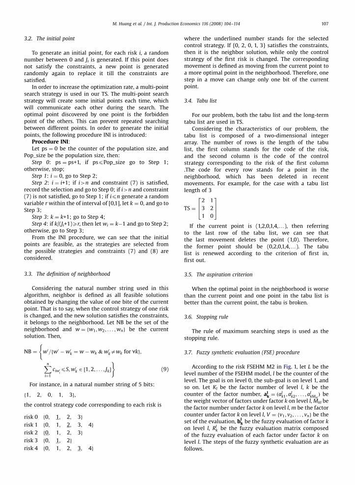
Considering the project organization mode and thefuzzy characteristics of a VE, the objective of the modelM1 is obtained by the fuzzy synthetic evaluation hier-archical model (FSEHM) M2 of risk evaluation, which isgiven in Fig. 1. In this FSEHM model, each process of the VEproject is considered, as well as the fuzzy description ofeach risk factor.

In the FSEHM model, there are 5 levels, from level 0(top) to level 4 (bottom). Level 0, which correspondsto the objective of model M1, is the goal of a VE. Level 1consists of the sub-goals pursued by the VE, whichare different for a special VE. Level 2 consists of theprocesses, which are the activities in the VE project.Level 3 is made up of the risk events, which will cause therisk in the processes for different sub-goals. Level 4 isthe risk factors of the risk event. For a VE, the fuzzydescription of these factors with different control strate-gies is assumed to be known and is described as thedegree of membership to each ranking of risk. The riskranks are given in Table 1. Also, the relative weights of thelower-level factors to the upper-level factors are assumedto be known.

It can be seen in Fig. 1, that the risk evaluation isconducted from the local system (lowest level) to theglobal system (level 0). The level of fuzzy global risk forcertain risk programming solutions can be obtained by thefuzzy synthetic evaluation (Lu et al., 1999).

The risk at the global level can then be determinedaccording to the rule of the maximum degree of member-ship according to the level of fuzzy global risk. However,using this method, many solutions may have the samelevel of global risk, as shown in Fig. 2, where d is the riskrank, and a is the membership degree.

According to the rule of the maximum degree ofmembership, the global risk level of the two solutions inFigs. 2(a) and (b) are same, at 4. However, the risk state ofFig. 2(a) is better than that of Fig. 2(b) taking intoconsideration all of the degrees of membership of thesesolutions, which cannot be shown according to the rule ofthe maximum degree of membership. Therefore, consid-ering the membership degree and risk states, the objective

ARTICLE IN PRESS

Table 1Definition of risk ranks

Risk

rank

0 1 2 3 4 5 6 7 8

Risk

level

None Smallest Smaller Small Medium More Big Bigger Biggest

α

d 0.5/4 0.1/60.4/5

α

d0.5/4 0.2/60.3/5

Fig. 2. The fuzzy synthetic evaluation value of different solutions.

Goal

Sub-goal 1 Sub-goal 2 Sub-goal 3

process a process b process c

Risk event i Risk event j Risk event k

Level 0 Goal

Sub-goal 1 Sub-goal 2 Sub-goal 3

process a process b process c

Risk event j Risk event k

Risk factor x Risk factor y

M2:

Level 1

Level 2

Level 3

Level 4

Fig. 1. The hierarchical model for evaluating risk.

M. Huang et al. / Int. J. Production Economics 116 (2008) 104–114106

is modified as follows:

minXQ

q¼1

dpqa

pqðxÞ

!(5)

where q is the risk ranking, Q is the number of rankings ofrisks, and p is an integer larger than 0.

However, if p is set to an integer larger than 1 informula (5), the global risk level of the solutions inFig. 2(a) will be larger than that in Fig. 2(b) accordingly,which is not the case. So, 1 is selected for p in our analysis.

3. Algorithm design

Eqs. (1)–(4) are a hybrid of the combination problemand integer programming. The size of the solution space(the number of feasible solutions) of problem (1)–(4)can be determined by the number of risks and controlstrategies for the risks, which is

Qni¼1C1

Jiþ1 with noconstraints. It is easy to see that the problem is NP-hard.Therefore, the heuristic algorithm of this problem isneeded for practical use.

The tabu search (TS) algorithm is an effective methodfor solving large-scale combination optimization problem

and integer programming problems. The common heur-istic algorithms only adapt to special problems and easilysink into local optimal solutions. The TS algorithm canovercome this shortcoming. It has been used on anincreasing number of practical problems and has provento be effective (Glover, 1989, 1990).

3.1. The coding scheme and model transformation

For our TS, the natural number string is selected as thecode description. Let w ¼ fw1;w2; . . . ;wng, where wi is aninteger between 0 and Ji, 8i. This stands for that thecontrol strategy wi is selected for risk event i. Thus, w ¼

fw1;w2; . . . ;wng refers to a strategy selection. For example,a natural number string of 10 bits:

f1; 3; 4; 2; 2; 2; 3; 3; 3; 0g

is a strategies selection of 10 risk events. This means thatthe control strategy 1 for risk event 1, the control strategy3 for risk event 2, and so on, are selected. It should benoted that bit 10, 0 means that no strategy of risk 10 isselected. Not all of the risks are controlled in a riskprogramming solution due to limited cost investment inrisk control.

Objective (1) and constraints (2)–(4) are then equiva-lent to the following optimization problem:

min RðwÞ ¼XQ

q¼1

dqaqðwÞ

!(6)

s:t:Xn

i¼1

ciwipS (7)

wi 2 ½0;1; . . . ; Ji�; i ¼ 1;2; . . . ;n (8)

We can see that the rewritten model (6)–(8) is muchsimpler than the original model (1)–(4), but that there aresome variables in its subscripts. It is difficult to treat thisproblem using the traditional mathematical model, buteasy using a TS.

ARTICLE IN PRESS


3.2. The initial point

To generate an initial point, for each risk i, a randomnumber between 0 and Ji is generated. If this point doesnot satisfy the constraints, a new point is generatedrandomly again to replace it till the constraints aresatisfied.

In order to increase the optimization rate, a multi-pointsearch strategy is used in our TS. The multi-point searchstrategy will create some initial points each time, whichwill communicate each other during the search. Theoptimal point discovered by one point is the forbiddenpoint of the others. This can prevent repeated searchingbetween different points. In order to generate the initialpoints, the following procedure INI is introduced:

Procedure INI:Let ps ¼ 0 be the counter of the population size, and

Pop_size be the population size, then:Step 0: ps ¼ ps+1, if pspPop_size go to Step 1;

otherwise, stop;Step 1: i ¼ 0, go to Step 2;Step 2: i ¼ i+1; if i4n and constraint (7) is satisfied,

record the selection and go to Step 0; if i4n and constraint(7) is not satisfied, go to Step 1; if ipn generate a randomvariable r within the of interval of [0,1], let k ¼ 0, and go toStep 3;

Step 3: k ¼ k+1; go to Step 4;Step 4: if k/(Ji+1)Xr, then let wi ¼ k�1 and go to Step 2;

otherwise, go to Step 3;From the INI procedure, we can see that the initial

points are feasible, as the strategies are selected fromthe possible strategies and constraints (7) and (8) areconsidered.

3.3. The definition of neighborhood

Considering the natural number string used in thisalgorithm, neighbor is defined as all feasible solutionsobtained by changing the value of one bite of the currentpoint. That is to say, when the control strategy of one riskis changed, and the new solution satisfies the constraints,it belongs to the neighborhood. Let NB be the set of theneighborhood and w ¼ fw1;w2; . . . ;wng be the currentsolution. Then,

NB ¼ w0=fw0 �w0k ¼ w�wk & w0kawk for 8kg;

(

Xn

i¼1

ciw0ipS;w0k 2 ½1;2; . . . ; Jk�

)(9)

For instance, in a natural number string of 5 bits:

f1; 2; 0; 1; 3g,

the control strategy code corresponding to each risk is

risk 0 f0; 1; 2; 3g

risk 1 f0; 1; 2; 3; 4g

risk 2 f0; 1; 2; 3g

risk 3 f0; 1; 2g

risk 4 f0; 1; 2; 3; 4g

where the underlined number stands for the selectedcontrol strategy. If {0, 2, 0, 1, 3} satisfies the constraints,then it is the neighbor solution, while only the controlstrategy of the first risk is changed. The correspondingmovement is defined as moving from the current point toa more optimal point in the neighborhood. Therefore, onestep in a move can change only one bit of the currentpoint.

3.4. Tabu list

For our problem, both the tabu list and the long-termtabu list are used in TS.

Considering the characteristics of our problem, thetabu list is composed of a two-dimensional integerarray. The number of rows is the length of the tabulist, the first column stands for the code of the risk,and the second column is the code of the controlstrategy corresponding to the risk of the first column.The code for every row stands for a point in theneighborhood, which has been deleted in recentmovements. For example, for the case with a tabu listlength of 3

TS ¼

2 1

3 2

1 0

264

375

If the current point is (1,2,0,1,4,y), then referringto the last row of the tabu list, we can see thatthe last movement deletes the point (1,0). Therefore,the former point should be (0,2,0,1,4,y). The tabulist is renewed according to the criterion of first in,first out.

3.5. The aspiration criterion

When the optimal point in the neighborhood is worsethan the current point and one point in the tabu list isbetter than the current point, the tabu is broken.

3.6. Stopping rule

The rule of maximum searching steps is used as thestopping rule.

3.7. Fuzzy synthetic evaluation (FSE) procedure

According to the risk FSEHM M2 in Fig. 1, let L be thelevel number of the FSEHM model, l be the counter of thelevel. The goal is on level 0, the sub-goal is on level 1, andso on. Let Kl be the factor number of level l, k be thecounter of the factor number, al

k ¼ ðalk1; a

lk2; . . . ; a

lkMklÞ be

the weight vector of factors under factor k on level l, Mkl bethe factor number under factor k on level l, m be the factorcounter under factor k on level l, V ¼ fv1; v2; . . . ; vng be theset of the evaluation, bl

k be the fuzzy evaluation of factor k

on level l, Rlk be the fuzzy evaluation matrix composed

of the fuzzy evaluation of each factor under factor k onlevel l. The steps of the fuzzy synthetic evaluation are asfollows.

ARTICLE IN PRESS

Table 2The weight of the sub-goals to the goal

Sub-goal Cost Coordination Time Quality

Weight 0.3 0.3 0.15 0.25


Procedure FSE:Step 1: l ¼ L�2; k is from 1 to Kl; determine Rl

k

according to V, then:

blk ¼ al

k � Rlk ¼ ðb

lk1bl

k2; . . . ; blknÞ ðk ¼ 1;2; . . . ;KlÞ (10)

The synthetic evaluation of level l is finished; and turnsto Step 2.

Step 2: If l ¼ 0, stop. Otherwise, let l ¼ l�1, and turn toStep 3.

Step 3: Let k be from 1 to Kl, according toblþ1

m ¼ ðblþ1m1 blþ1

m2 ; . . . ; blþ1mn Þðm ¼ 1;2; . . . ;MklÞ, Rl

k is givenas follows:

Rlk ¼

blþ11

blþ12

..

.

blþ1Mkl

8>>>>>><>>>>>>:

9>>>>>>=>>>>>>;¼

blþ111 blþ1

12 � � � blþ11n

blþ121 blþ1

22 � � � blþ12n

� � � � � � � � � � � � � � � � � �

blþ1Mkl1

blþ1Mkl2

� � � blþ1Mkln

8>>>>><>>>>>:

9>>>>>=>>>>>;

(11)

Then, according to Eq. (10) the synthetic evaluation oflevel l is finished. Turns to Step 2.

In Eq. (10), the weighted-mean-determining type isused as the compound calculation in the fuzzy metric asshown in Eq. (12).

blkj ¼

XMkl

i¼1

alkib

lþ1ij ; j ¼ 1;2; . . . ;n; k ¼ 1;2; � � � ;Kl (12)

3.8. The procedure for the FSE-embedded-TS (fuzzy synthetic

evaluation embedded tabu search)

The step-by-step procedure of the FSE-embedded-TS isas follows:

Procedure FSE-embedded-TS:Step 1: Specify the parameters:Pop_size is the number of initial points, Step is the

number of search steps.Step 2: Generate an initial population with Pop_size

points using Procedure INI,

wðjÞ ¼ ½w1ðjÞ;w2ðjÞ; . . . ;wnðjÞ�; j ¼ 1;2; . . . ;Pop_size.

Set the search index to k ¼ 0. For point wðjÞ; j ¼

1;2; . . . ;Pop_size, call Procedure OBJ. Then the initialoptimal solution w* ¼ wj* and the optimal objectivefunction value R* ¼ Rj*.

Step 3: Let k ¼ k+1. If k4Step, go to Step 7, otherwise,implement Steps 4–6.

Step 4: For point wðjÞ; j ¼ 1;2; . . . ;Pop_size, generateneighborhood NB according to Eq. (9). Go to Step 5.

1

3

4

2Lamp design

Cap manufacturing

Bulb manufacturing

Core manufa

Fig. 3. The network for la

Step 5: To generate the new population wðjÞ; j ¼

1;2; . . . ;Pop_size, considering the tabu list, the long-termtabu list, the aspiration criterion, and the constraint (7).Go to Step 6.

Step 6: Call Procedure OBJ. If RminoRn, let R* ¼ Rmin andw* ¼ w(j*).

Step 7: Output R* and w* is the optimal solution.Procedure OBJ:Step 1: Call Procedure FSE calculates the global risk

level and returns the value of R(j) and the total costCðjÞ ¼

Pni¼1ciwiðjÞ.

Step 2: Find Rmin ¼ minPop_sizefRðjÞ=CðjÞpSg. Then, jn ¼

argfRðjÞ ¼ Rming is the index of Rmin that was achieved andthe associated control strategy that was selected.

4. Simulation study

4.1. The example

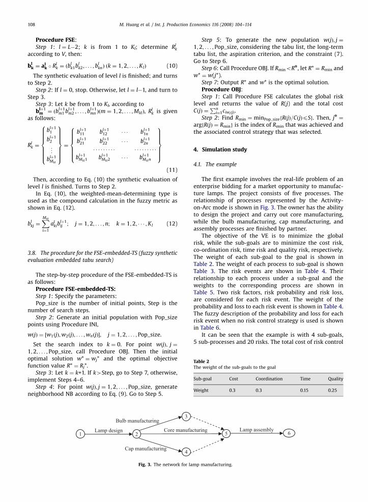
The first example involves the real-life problem of anenterprise bidding for a market opportunity to manufac-ture lamps. The project consists of five processes. Therelationship of processes represented by the Activity-on-Arc mode is shown in Fig. 3. The owner has the abilityto design the project and carry out core manufacturing,while the bulb manufacturing, cap manufacturing, andassembly processes are finished by partner.

The objective of the VE is to minimize the globalrisk, while the sub-goals are to minimize the cost risk,co-ordination risk, time risk and quality risk, respectively.The weight of each sub-goal to the goal is shown inTable 2. The weight of each process to sub-goal is shownTable 3. The risk events are shown in Table 4. Theirrelationship to each process under a sub-goal and theweights to the corresponding process are shown inTable 5. Two risk factors, risk probability and risk loss,are considered for each risk event. The weight of theprobability and loss to each risk event is shown in Table 4.The fuzzy description of the probability and loss for eachrisk event when no risk control strategy is used is shownin Table 6.

It can be seen that the example is with 4 sub-goals,5 sub-processes and 20 risks. The total cost of risk control

5 6cturing Lamp assembly

mp manufacturing.

ARTICLE IN PRESS

Table 3The weight (w) of the processes to the sub-goals

Sub-goal Process

Lamp design Bulb manufacturing Core manufacturing Cap manufacturing Lamp assembly

Cost 0.5 0.3 0.05 0.15 0

Coordination 0.2 0.5 0.1 0.1 0.1

Time 0 0.2 0.3 0.3 0.2

Quality 0 0 0.4 0.6 0

Table 4The risk events and their probability and loss weight

Risk

event no.

Risk event Risk

probability

Risk

loss

1 Design method 0.4 0.6

2 Designer’s level 0.5 0.5

3 Delay of bulb 0.4 0.6

4 Bad rate of core 0.35 0.65

5 Delay of cap 0.5 0.5

6 Communication with the partner 0.35 0.65

7 Selection of the bulb partner 0.8 0.2

8 Contract award 0.15 0.85

9 Strategy of the partner 0.25 0.75

10 Selection of the cap partner 0.3 0.7

11 Selection of the assembly partner 0.7 0.3

12 The experience of the designer 0.5 0.5

13 The complexity of the product 0.6 0.4

14 Contract management 0.8 0.2

15 The capability of the enterprise 0.3 0.7

16 The experience of the worker 0.7 0.3

17 The capability of the assembly

partner

0.5 0.5

18 The reputation of the bulb partner 0.2 0.8

19 The reputation of the cap partner 0.65 0.35

20 The reputation of the assembly

partner

0.5 0.5


is 20,000 RMB. The cost of the control strategy for eachrisk is shown in Table 7, where the highlighted recordstands for the selected strategy of optimal solution. Thenumber of the control strategy (including the no controlone) for each risk is shown in Table 8. It is clear that thereare 96,745,881,600 solutions for this problem withoutconstraints.

4.2. Parameters setting of TS

The setting of the values of various parameters in theTS algorithm is important for the efficiency of thealgorithm. Therefore, the turning of the parameters ofthe TS for the problem is presented in this section. Theparameters considered are the number of initial points(the population size) ‘‘Pop_size’’, the search steps of thealgorithm ‘‘Step’’, the length of the tabu list ‘‘Tabu_size’’,and the length of the long-term tabu list ‘‘Long’’.

In the analysis, the performance used to tune theparameters is the ‘‘Best_rate’’, where ‘‘Best’’ stand for thebest one of the objective values achieved in 100 runs.The ‘‘Best_rate’’ is the rate to reach the best value. Thealgorithm was run 100 times with different randomseeds for each parameter setting to test the random effect

on the solution. Therefore, the parameters with highest‘‘Best_rate’’ are better than others.

(1)
The effect of the length of the tabu list on the‘‘Best_rate’’.
The analysis on the effect of the length of the tabu liston the ‘‘Best_rate’’ is shown in Table 9. The ‘‘Cyc_rate’’is also used in this analysis, where ‘‘Cyc’’ stand for thedead cycle occurred in each of the 100 runs. When thedead cycle occurs, the TS algorithm will loss its‘‘climb’’ ability. The ‘‘Cyc_rate’’ means the rate thedead cycle occurred in 100 runs. It shows that‘‘Best_rate’’ and ‘‘Cyc_rate’’ vary regularly with thelength of the tabu list. As the length of the tabu listincreases, the ‘‘Cyc_rate’’ decrease, but the ‘‘Best_rate’’first increases and then decreases. This is because, thelonger the tabu list is, the more points are forbiddenand the fewer chances there are to return into the lastpoint. Therefore, the algorithm has a stronger ‘‘climb’’ability. But, a tabu list that is too long will cause the‘‘Best_rate’’ to decline. Obviously, if the algorithm isgoing to solve the combinatorial optimization pro-blem, the longer the tabu list is, the more points areforbidden, and the fewer combination alternatives canbe chosen; therefore, we have fewer chances to obtainthe optimal point. Moreover, the longer the tabu list is,the lower the ‘‘Cyc_rate’’ is. Considering the columnsof ‘‘Cyc_rate’’ and ‘‘Best_rate’’, it is easy to see that ifthe length of the tabu list is appropriate, there is lessof a chance that the search will go to the dead cycle,and the ‘‘Best_rate’’ will be higher. Hence, the deadcycle is one factor affecting the ‘‘Best_rate’’, when thetabu list is of an appropriate length. In order todecrease the ‘‘Cyc_rate’’, the long-term tabu list isused in this research. The long-term tabu list is able toremember recent moves, and is used to detectwhether there is a cycle. If there is, the current pointwill move to the sub-optimal neighbor solution. Usingthis method, the cycle can be avoided. However, it isnot necessary to detect whether there is a cycle foreach step of movement. Therefore, the length of thelong-term tabu list is the other factor affecting the‘‘Best_rate’’.Table 9 also shows that the reasonable length of thetabu size is 8.

(2)
The effect of the length of the long-term tabu liston the ‘‘Best_rate’’.The effect of the length of the long-term tabu list onthe ‘‘Best_rate’’ is shown in Table 10. It illustrates that

ARTICLE IN PRESS

Table 5The relationship and weight of the risk event to the processes under the sub-goals

Sub-goal Process

Lamp design Bulb manufacturing Core manufacturing Cap manufacturing Lamp assembly

Cost Risk 1 (0.7) Risk 3 (1.0) Risk 4 (1.0) Risk 5 (1.0) –

Risk 2 (0.3)

Coordination Risk 6 (1.0) Risk 7 (0.5) – Risk 10 (1.0) Risk 11 (1.0)

Risk 8 (0.4)

Risk 9 (0.1)

Time Risk 12 (0.2) Risk 14 (1.0) Risk 15 (0.8) – Risk 17 (1.0)

Risk 13 (0.8) Risk 16 (0.2)

Quality – Risk 18 (1.0) – Risk 19 (1.0) Risk 20 (1.0)

Table 6The fuzzy description of the probability and loss for each risk event with no risk control

Risk event Risk rank

0 1 2 3 4 5 6 7 8

1 Probability 0.0 0.0 0.0 0.3 0.5 0.2 0.0 0.0 0.0

Loss 0.0 0.0 0.0 0.0 0.2 0.8 0.0 0.0 0.0

2 Probability 0.0 0.0 0.3 0.3 0.3 0.1 0.0 0.0 0.0

Loss 0.0 0.0 0.0 0.0 0.3 0.5 0.2 0.0 0.0

3 Probability 0.0 0.0 0.1 0.2 0.4 0.3 0.0 0.0 0.0

Loss 0.0 0.3 0.4 0.3 0.0 0.0 0.0 0.0 0.0

4 Probability 0.0 0.0 0.0 0.0 0.0 0.6 0.4 0.0 0.0

Loss 0.0 0.0 0.0 0.2 0.6 0.2 0.0 0.0 0.0

5 Probability 0.0 0.0 0.1 0.2 0.4 0.3 0.0 0.0 0.0

Loss 0.0 0.3 0.4 0.3 0.0 0.0 0.0 0.0 0.0

6 Probability 0.0 0.0 0.0 0.5 0.5 0.0 0.0 0.0 0.0

Loss 0.0 0.0 0.0 0.5 0.5 0.0 0.0 0.0 0.0

7 Probability 0.0 0.0 0.0 0.3 0.4 0.3 0.0 0.0 0.0

Loss 0.0 0.0 0.1 0.2 0.3 0.3 0.1 0.0 0.0

8 Probability 0.0 0.0 0.1 0.8 0.1 0.0 0.0 0.0 0.0

Loss 0.0 0.0 0.1 0.8 0.1 0.0 0.0 0.0 0.0

9 Probability 0.0 0.5 0.5 0.0 0.0 0.0 0.0 0.0 0.0

Loss 0.0 0.5 0.5 0.0 0.0 0.0 0.0 0.0 0.0

10 Probability 0.0 0.0 0.0 0.0 0.3 0.4 0.3 0.0 0.0

Loss 0.0 0.8 0.2 0.0 0.0 0.0 0.0 0.0 0.0

11 Probability 0.0 0.1 0.3 0.5 0.1 0.0 0.0 0.0 0.0

Loss 0.0 0.0 0.0 0.4 0.4 0.2 0.0 0.0 0.0

12 Probability 0.0 0.0 0.5 0.5 0.0 0.0 0.0 0.0 0.0

Loss 0.0 0.0 0.0 0.3 0.5 0.2 0.0 0.0 0.0

13 Probability 0.0 0.0 0.4 0.3 0.3 0.0 0.0 0.0 0.0

Loss 0.0 0.0 0.6 0.2 0.2 0.0 0.0 0.0 0.0


ARTICLE IN PRESS

Table 6 (continued )

Risk event Risk rank

0 1 2 3 4 5 6 7 8

14 Probability 0.0 0.0 0.0 0.5 0.5 0.0 0.0 0.0 0.0

Loss 0.0 0.0 0.0 0.5 0.5 0.0 0.0 0.0 0.0

15 Probability 0.0 0.0 0.4 0.3 0.3 0.0 0.0 0.0 0.0

Loss 0.0 0.0 0.0 0.4 0.4 0.2 0.0 0.0 0.0

16 Probability 0.0 0.0 0.3 0.3 0.3 0.1 0.0 0.0 0.0

Loss 0.0 0.0 0.0 0.0 0.3 0.5 0.2 0.0 0.0

17 Probability 0.0 0.0 0.0 0.0 0.0 0.2 0.4 0.4 0.0

Loss 0.0 0.0 0.5 0.5 0.0 0.0 0.0 0.0 0.0

18 Probability 0.0 0.0 0.3 0.3 0.2 0.2 0.0 0.0 0.0

Loss 0.0 0.0 0.0 0.2 0.2 0.2 0.4 0.0 0.0

19 Probability 0.0 0.0 0.0 0.0 0.0 0.6 0.4 0.0. 0.0

Loss 0.0 0.0 0.00 0.2 0.6 0.2 0.0 0.0 0.0

20 Probability 0.0 0.8 0.2 0.0 0.0 0.0 0.0 0.0 0.0

Loss 0.0 0.0 0.0 0.0 0.3 0.5 0.2 0.0 0.0

Table 7Control strategy cost for each risk

Risk Strategy Cost

Risk 1 Strategy 1 1000

Strategy 2 2000


Strategy 2 5000

Strategy 3 500


Strategy 2 2000

Strategy 3 3000


Strategy 2 2000

Strategy 3 1000

Strategy 4 3000


Strategy 2 2000

Strategy 3 3000


Strategy 2 1000

Strategy 3 1000


Strategy 2 2000


Strategy 2 3000

Strategy 3 2000


Strategy 2 3000


Risk Strategy Cost

Strategy 3 2000


Strategy 2 2000


Strategy 2 5000


Strategy 2 2000


Strategy 2 3000


Strategy 2 500

Strategy 3 500


Strategy 2 5000


Strategy 2 2000

Strategy 3 3000


Strategy 2 5000


Strategy 2 3000


Strategy 2 2000


ARTICLE IN PRESS


Risk Strategy Cost

Strategy 3 500

Strategy 4 1000


Strategy 2 5000

Table 8The number of risk control strategy for each risk (problem 1)

Risk 1 2 3 4 5 6 7 8 9 10 11 12 13 14 15 16 17 18 19 20

Strategy

number 3 4 4 5 4 4 3 4 4 3 3 3 3 4 3 4 3 3 5 3

Table 9The effect of the tabu list length on the ‘‘Best_rate’’

Pop_size Step Tabu_size Long Cyc_rate (%) Best_rate (%)

1 1000 3 No 100 16

1 1000 5 No 84 17

1 1000 7 No 71 15

1 1000 8 No 29 47

1 1000 9 No 72 29

1 1000 10 No 31 41

1 1000 11 No 23 33

1 1000 12 No 7 43

1 1000 13 No 0 35

1 1000 15 No 0 22

1 1000 17 No 0 11

*‘‘No’’ stand for no long tabu list is used.

Table 10The effect of the length of a long-term list on the ‘‘Best_rate’’

Pop_size Step Tabu_size Long Best_rate (%)

1 1000 3 No 16

1 1000 3 10 16

1 1000 3 20 16

1 1000 3 30 16

1 1000 3 40 16

1 1000 7 No 15

1 1000 7 10 27

1 1000 7 20 23

1 1000 7 30 23

1 1000 7 40 24

1 1000 8 No 47

1 1000 8 10 49

1 1000 8 20 48

1 1000 8 30 48

1 1000 8 60 49

1 1000 8 80 48

1 1000 8 100 47

1 1000 9 No 29

1 1000 9 10 44

1 1000 9 20 40

1 1000 9 30 41

1 1000 9 60 37

1 1000 9 80 37

1 1000 9 100 31

TablThe

Pop_

1

5

TablThe

Risk

Strat

Risk

Strat

TablThe

Pop_

5

5

5

5


the effect of the long-term tabu list on the ‘‘Best_rate’’is closely related with the length of the tabu list.A tabu list that is too short (e.g., where the length ofthe tabu list is 3) will leads to a long-term tabu listthat is of no use. This is because even though the long-term tabu list can detect the cycle and adjust it in atimely manner, it is still not able to prevent the searchfalling to the cycle again. When the tabu list is of anappropriate length, the long-term tabu list will have abetter effect.In addition, we can see from Table 10 that, using along-term tabu list can increase the ‘‘Best_rate’’ byavoiding the cycles, although a long-term tabu list hasan auxiliary effect on the tabu list. A reasonable lengthfor a long-term tabu list is 80.

(3)
The effect of the size of the population on the‘‘Best_rate’’.The effect of the size of the population on the‘‘Best_rate’’ is shown in Table 11. The results showthat one initial point leads to an unfavorable result.This is because some initial points do not lead to theoptimal point, but to local optimal ones. Hence, theless random initial point leads to a low ‘‘Best_rate’’.The multi-point search strategy can overcome thisshortcoming. As is shown in Table 11, the datasuggests that the multi-point search strategy causesan obvious increase in the ‘‘Best_rate’’, and 5 is thesuggested population number. A larger populationsize will only require more search time, but lead to noimprovement to the solution.
e 11effect of the number of initial points on the ‘‘Best_rate’’

size Step Tabu_size Long Best_rate (%)

1000 8 80 48

1000 8 80 95

e 13number of risk control strategies for each risk (problem 2)

1 2 3 4 5 6 7 8 9 10 11 12 13 14 15

egy number 4 4 5 5 3 4 3 3 3 4 3 3 5 4 3

16 17 18 19 20 21 22 23 24 25 26 27 28 29 30

egy number 3 2 2 4 4 4 3 2 3 4 4 4 4 3 3

e 12effect of the number of search steps on the ‘‘Best_rate’’

size Step Tabu_size Long Best_rate (%)

300 8 80 86

500 8 80 90

1000 8 80 95

1500 8 80 95

ARTICLE IN PRESS

Table 14The effect of the problem scale on the Best_rate

Problem scale Pop_size Step Tabu_size Long Best_rate(%) CPU time (s)

96,745,881,600 5 1000 8 80 95 5.7

8,916,100,448,256,000 5 1000 8 80 93 6.5


(4)
The effect of the number of search steps on the‘‘Best_rate’’.The effect of the number of search steps on the‘‘Best_rate’’ is shown in Table 12. The data in the tablesuggests that 1000 is a proper number of search stepsfor the problem. Less search steps will lead to thedecrease of the ‘‘Best_rate’’, however, more searchsteps will only lead to more time consumed but withno increase of the ‘‘Best_rate’’.The above analysis has shown that the number ofinitial points ‘‘Pop_size’’ ¼ 5, the number of searchsteps ‘‘Step’’ ¼ 1000, the length of the tabu list‘‘Tabu_size’’ ¼ 8, and the length of the long-term tabulist ‘‘Long’’ ¼ 80 are a reasonable combination ofparameters for this problem. The effect of the problemscale on the algorithm is then studied.
(5)
The effect of the problem scale on the ‘‘Best_rate’’.In order to analyze the effect of the problem scale onthe ‘‘Best_rate’’, according to the former example, wereset the problem scale with 5 sub-goals, 5 sub-processes and 30 risks. The control strategy (includingthe no control one) number for each risk is shown inTable 13.
There are 8,916,100,448,256,000 solutions for thisexample without constraints, which is 92,160 times
more than the first example. Using the reasonableparameter combination, the optimal rate is given inTable 14.
As is shown in Table 14, the problem scale growsextremely rapidly with the risk number. The tabu searchalgorithm can achieve the optimal solution with a higherprobability but the computation time does not increasequickly with increase in problem size. In general, thesimulation suggests that the tabu search algorithm iseffective for this kind of problem.

5. Conclusions

Risk programming is a problem inherent in VEs.Minimizing total risk within the risk investment is thekey to ensuring the success of the VE. This paperintroduced a description of the risk programming problemof VEs. The fuzzy synthetic evaluation embedded non-linear integer programming model provides a formaldescription of the risk programming problem of VEs,where the following two features differentiating VEs fromconventional enterprises are considered:

�
The project organization mode. � The fuzzy information characteristics of VE.
An FSE-embedded-TS for this problem was proposed. Ithas better synthetic performance in terms of both
computation speed and optimality efficient. The simula-tion results suggest that it has the potential to solvepractical risk programming problems in VE.
In general, the proposed model and algorithm has thepotential to be an efficient quantitative tool for riskmanagement in the virtual global business environment.

Acknowledgments

The authors wish to thank the support of the NationalNatural Science Foundation of China (Project nos.70671020, 70721001, 70431003, 60673159), NationalHigh-Tech Research and Development Plan of China(Project no. 2006AA01Z214), the Program for New CenturyExcellent Talents in University (Project nos. NCET-05-0295, NCET-05-0289), Specialized Research Fund for theDoctoral Program of Higher Education (Project no.20070145017); the Hong Kong Polytechnic Universityfoundation (Project no. A-PA1K).

References

Ayyub, B.M., 2003. Risk Analysis in Engineering and Economics.Chapman & Hall/CRC, Boca Raton, FL.

Bernus, P., Nemes, L., 1999. Organisational design: Dynamically creatingand sustaining integrated virtual enterprises. In: Chen, H.-F., Cheng,D.-Z., Zhang, J.-F. (Eds.), Proceedings of IFAC World Congress, vol. A.Elsevier, London.

Bier, V.M., Haimes, Y.Y., Lambert, J.H., Matalas, N.C., Zimmerman, R., 1999.Survey of approaches for assessing and managing the risk ofextremes. Risk Analysis 19 (1), 83–94.

Fan, M., Lin, N.-P., Sheu, C., 2008. Choosing a project risk-handlingstrategy: An analytical model. International Journal of ProductionEconomics 112 (2), 700–713.

Glover, F., 1989. Tabu search: Part I. ORSA Journal on Computing 1 (3),190–206.

Glover, F., 1990. Tabu search: Part II. ORSA Journal on Computing 2 (1),4–32.

Haimes, Y.Y., 2004. Risk Modeling, Assessment, and Management, seconded. Wiley, New York.

Hallikas, J., Karvonen, I., Pulkkinen, U., Virolainen, V-M., Tuominen, M.,2004. Risk management processes in supplier networks. Interna-tional Journal of Production Economics 90 (1), 47–58.

Ip, W.H., Huang, M., Yung, K.L., Wang, D., 2003. Genetic algorithmsolution for a risk-based partner selection problem in a virtualenterprise. International Journal of Computers and OperationsResearch 30 (2), 213–231.

Kliem, R.L., Ludin, I.S., 1997. Reducing Project Risk. Gower PublishingLimited, England.

Lu, R.S., Lo, S.L., Hu, J.Y., 1999. Analysis of reservoir water quality usingfuzzy synthetic evaluation. Stochastic Environmental Research andRisk Assessment 13 (5), 327–336.

Makatsoris, C., Leach, N.P., Richards, H.D., Ristic, M., Besant, C.B., 1996.Addressing the planning and control gaps in semiconductor virtualenterprises. In: Proceedings of the Conference on Integration inManufacturing. Galway, Ireland, pp. 117–129.

ARTICLE IN PRESS


Park, K.H., Favrel, J., 1999. Virtual enterprise-information system andnetworking solution. Computers and Industrial Engineering 37 (1),441–444.

Treleven, M., Schweikhart, S.B., 1988. A risk/benefit analysis of sourcingstrategies: Single vs. multiple sourcing. Journal of OperationsManagement 7 (4), 93–114.

Virolainen, V.-M., Tuominen, M., 1998. Hankintatoimeen liittyvaK t riskitteollisuusyrityksessaK. In: Kuusela, H., Ollikainen, R. (Eds.), Riskit jaRiskienhallinta. University Press, Nancy, pp. 164–178.

Wang, S., Tang, X., 2002. Research on risk and income for diversifiedoperation of virtual enterprise. Operations Research and Manage-ment Science 11 (4), 1–4.

a fuzzy synthetic evaluation embedded tabu search for risk programming of virtual enterprises

Documents