a fundamental limits of cyber-physical systems … · equations that describe the semiconductor...

A

Fundamental Limits of Cyber-Physical Systems Modeling1

EDWARD A. LEE, EECS Department, UC Berkeley

This paper examines the role of modeling in the engineering of cyber-physical systems. It argues that the

role that models play in engineering is different from the role they play in science, and that this difference

should direct us to use a different class of models, where simplicity and clarity of semantics dominate overaccuracy and detail. I argue that determinism in models that are used for engineering is a valuable property

and should be preserved whenever possible, regardless of whether the system being modeled is deterministic.

I then identify three classes of fundamental limits on modeling, specifically chaotic behavior, the inabilityof computers to numerically handle a continuum, and the incompleteness of determinism. The last of these

has profound consequences.

1. MODELING

Modeling is central to every scientific and engineering enterprise. Golomb, who has writteneloquently about the use of models in science and engineering, emphasizes understandingthe distinction between a model and thing being modeled. He famously stated “you willnever strike oil by drilling through the map” [Golomb 1971].

For both scientists and engineers, the “thing being modeled” is typically an object, pro-cess, or system in the physical world. But it could also be another model. Let us call thething being modeled the target of the model. The fidelity of a model is the degree towhich it emulates the target.

When the target is a physical object, process, or system, then model fidelity is neverperfect. Box and Draper state, “essentially, all models are wrong, but some are useful” [Boxand Draper 1987]. In science, the value of a model lies in how well its properties match thoseof the target. In engineering, however, the value of the target lies in how well its propertiesmatch those of the model. A scientist constructs models in order to help understand thetarget. An engineer constructs targets to emulate the properties of a model. For an engineer,a model provides a design and the target is the implementation.

These two uses of models are complementary. An engineer will typically use models bothways. Good engineering requires doing some science. And at least for experimental science,good science requires doing some engineering.

Although model fidelity is rarely perfect, some models are astonishingly good. A syn-chronous digital circuit, which is a collection of gates and latches that are clocked, is amodel of physical system, a three-dimensional structure of doped semiconductors with anapplied voltage. The modeling paradigm of synchronous digital circuits is simple, rooted inboolean logic, and (often, but not always) deterministic; if you know the initial state of thecircuit and you know the inputs, then there is exactly one behavior specified by the model.Humans have learned to build targets that match the behavior of such models extremelywell. We can build a chip that will perform an operation specified by a synchronous digitallogic model a billion times per second, and the chip will very likely function without errorfor years. No other human-engineered artifact has ever reached this level of model fidelity.

A given target may have many useful models. For example, a microprocessor chip maybe modeled as a three-dimensional geometry of doped silicon (model A); as differential

1This paper reflects several years of work under several sponsored projects, including: the TerraSwarmResearch Center, one of six centers administered by the STARnet phase of the Focus Center ResearchProgram (FCRP) a Semiconductor Research Corporation program sponsored by MARCO and DARPA; theiCyPhy Research Center (Industrial Cyber-Physical Systems, supported by IBM and United Technologies);the National Science Foundation (NSF) awards #1446619 (Mathematical Theory of CPS), #1329759(COSMOI), #0931843 (ActionWebs), #0720882 (CSR-EHS: PRET), #1035672 (CPS: Medium: TimingCentric Software); and the Center for Hybrid and Embedded Software Systems (CHESS) at UC Berkeley,supported by the following companies: Denso, IHI, National Instruments, and Toyota.

ACM Journal Name, Vol. V, No. N, Article A, Publication date: January YYYY.

eal

Typewritten Text

To appear, ACM Tr. on Cyber-Physical Systems, 2016.

A:2 E. A. Lee

equations that describe the semiconductor physics (model B); as a synchronous digitalcircuit (model C); or as a computer program (model D) specifying embedded software forthe chip to run. These models are all abstractions of the chip, and they serve very differentpurposes. Which model to use depends on the goal.

Every model is constructed within some modeling framework that provides the syntaxby which the model is specified (how it is written down or otherwise rendered in physicalform) and the semantics (what a given rendition means). For example, model A mightbe given in a language for describing 3D shapes. Model B is given in the framework ofthe calculus of ordinary and partial differential equations. Model C is given in a hardwaredescription language, such as VHDL. Model D is given in a programming language.

The choice of modeling framework has profound consequences. For example, the languagefor describing 3D shapes (model A) is not well suited for modeling the dynamics of a circuit(how the voltages and currents change over time).

The properties of a modeling framework can also strongly affect the value of a modelin that framework. A framework intended for expressing dynamics, for example, may bedeterministic or not. In a deterministic framework, if the initial state of the model is known,and if the inputs to the model are known, then the model specifies exactly one behavior. Ina nondeterministic framework, the model specifies a family of behaviors.

Note that the role of inputs in a model overlaps with the role of nondeterminism. Modelsthat have inputs define a family of behaviors. A deterministic model defines one behaviorfor each possible input. Inputs are provided by the environment; they are not defined bythe model. Inputs can equally well be modeled as nondeterminism, but doing so reducesour ability to design a control system, which observes outputs in order to provide inputsthat drive towards some desired behavior.

Note that determinism is a property of a model, and not a property of the thing beingmodeled (unless that thing is also a model).2 Indeed, asserting determinism in the physicalworld would put us in the middle of a centuries-old debate in philosophy and physics, andit would probably require us to reject much of modern physics.

Determinism in models, however, has proved practical and extremely valuable in the past.Ordinary and partial differential equations, for example, are deterministic, and mechanical,electrical, and civil engineers rely heavily on that determinism. They use these equations todevelop controllers, to prove stability, and to analyze robustness to parameter variations.Synchronous digital circuit models are also (often) deterministic, as are single-threadedimperative programs. This determinism is hugely valuable, as it enables very complex andyet reliable designs by enabling definitive analysis. We can make absolute assertions aboutthe behavior of a deterministic model. No such assertions are possible about the physicalworld (how will the synchronous digital circuit behave while it’s being crushed?). The targetsof deterministic models, however, can only be deterministic if the target itself is a model.The lack of determinism in the physical world does not undermine the value of deterministicmodels as long as the model fidelity is high.

The determinism of a model depends on what is considered to be an output from themodel. For example, a terminating single-threaded imperative program is deterministic ifthe output is defined to be the final state of the machine. However, if we also consider thetime at which that final state is reached to be an output, then the model is nondeterministic.

Choosing to use deterministic models can have a cost. For example, by choosing to usesingle-threaded imperative programs, we forgo the ability to exploit the parallelism in amulticore machine. However, this cost is not a consequence of choosing determinism, it isa consequence of choosing this particular deterministic modeling framework. If we were tochoose instead to build our program using Kahn process networks [Kahn and MacQueen

2Here, I disagree with the position taken by Furia et al., who state “the notions of determinism andnondeterminism are attributes of the systems being modeled or analyzed” [Furia et al. 2010].


Fundamental Limits of Cyber-Physical Systems Modeling A:3

1977] or any of several other deterministic actor modeling frameworks, we would still beworking with deterministic models, and the execution of the software would have no diffi-culty exploiting multicore hardware.

Some problems may seem to require nondeterminism as a basic part of the problem state-ment. For example, if you are building a web server, requests will come in at random timesand may be very bursty. Implementing the web server as a single-threaded imperative pro-gram is probably not a good choice because every response to a request will be blocked bythe handling of all previous arrived requests. But again, we do not have to forgo determin-ism to handle these requests efficiently. We just have to forgo single-threaded imperativeprograms. All modern server-side software infrastructure includes support for simultaneousdispatch of multiple independent and mutually isolated request handlers. If the output ofthe server is defined to be the set of responses issued for a set of input requests, then it iseasy to provide a deterministic model of the server. If the output is defined instead to bea sequence of responses, then an efficient server will cannot be modeled deterministically.The order in which responses are issued is not a consequence of the inputs. If the designgoal is to issue predictable responses to requests, then a properly construed deterministicmodel is in fact valuable. For example, it can be used to specify regression tests.

1.1. Modeling Cyber-Physical Systems

A cyber-physical system (CPS) combines cyber systems (computational systems suchas microprocessors and digital communication networks) with other physical systems (elec-tromechanical, chemical, structural, and biological systems). Each of these components havebenefited from deterministic modeling frameworks, such as single-threaded imperative pro-grams and discrete-event models for the cyber side, and ordinary and partial differentialequations for the physical side. But as I have argued before in [Lee 2015], all widely usedcombinations of deterministic cyber models and deterministic physical models are nondeter-ministic. In the same paper I argued that this need not be so; deterministic models for CPSare practical. Given the evident value of determinism in modeling, deterministic frameworksshould be used.

In this paper, I reflect on lessons learned from building a deterministic modeling frame-work for cyber-physical systems called CyPhySim [Lee et al. 2015]. CyPhySim is an open-source simulator for CPS based on Ptolemy II [Ptolemaeus 2014]. CyPhySim supportsmixed continuous and discrete dynamics using a superdense model of time [Lee and Zheng2007], modal models and hybrid systems [Lee and Tripakis 2010], and an ability to importfunctional mockup units (FMUs) [Modelica Association 2014]. CyPhySim integrates fivesimulation engines:

(1) discrete event simulation (DE) [Lee 1999](2) quantized-state solvers (QSS) [Cellier and Kofman 2006](3) Runge-Kutta solvers (RK2-3, RK4-5) [Cellier and Kofman 2006](4) algebraic loop solvers [Lee et al. 2015](5) state machines [Feng et al. 2014]

This combination offers a rich set of modeling choices, and yet, some systems, even simplesystems, prove difficult to model in useful ways. This paper studies some of these difficultieswith a particular emphasis on identifying the fundamental limits of modeling. I focus onthree classes of fundamental limits:

(1) chaotic behavior,(2) the inability of computers to numerically handle a continuum, and(3) the incompleteness of determinism.

The first two of these are well known phenomena, so I focus on the implications they havefor CPS. The third, however, appears to be a relatively new observation, first made in [Lee


A:4 E. A. Lee

-20

-15

-10

-5

0

5

10

15

20

25

-15 -10 -5 0 5 10 15

Strange Attractor

x1x2

Fig. 1. Lorenz attractor executable model and a plot of x1 vs. x2 for an execution.

2014]. It implies that some classes of models have to admit nondeterminism. There is noway to avoid it.

2. CHAOS AND THE BUTTERFLY EFFECT

I have argued that determinism is a valuable property in models. A target in the physicalworld is not deterministic, but may nevertheless be usefully faithful to the model. Syn-chronous digital circuits and single-threaded imperative programs are excellent examples ofthis. Mechanical systems at scales where Newton’s laws work well are also good examples.

For a deterministic system, if the initial conditions, inputs, and parameters are knownprecisely, then the future behavior is known. This would seem to imply that deterministicsystems are predictable. But this is not really the case because of the caveat that the initialconditions, inputs and parameters need to be known precisely. If the model is chaotic, thenarbitrarily small perturbations in any of these can result in arbitrarily different behavior inthe future. This phenomenon is sometimes called the butterfly effect, invoking a metaphorthat the air movement caused by a butterfly wing may eventually cause a hurricane, in thatthe hurricane would not have occurred had the butterfly not flown.

Chaos often arises with non-linear feedback systems. A well-known example of such asystem is the Lorenz attractor, defined by the following set of differential equations:

x1(t) = σ(x2(t)− x1(t))

x2(t) = (λ− x3(t))x1(t)− x2(t) (1)

x3(t) = x1(t)x2(t)− bx3(t)

Augmented with initial conditions, these equations form a deterministic model. Anotherdeterministic model of the same system is shown in Figure 1. That model is a computationalmodel, a computer program (given with the graphical syntax of CyPhySim). It approximatesequations (1), and hence is a model whose target is another model. Despite the fact thatit approximates the other model, using Runge-Kutta or QSS numerical integration, it isnonetheless a deterministic model. How faithful is it to its target?

The answer to this question depends on how we measure the discrepancy between theidealized behavior of the differential equations and the computational model. In fact, mea-suring this discrepancy is difficult, because every computational model of the differential



equations will be “wrong” (in the Box and Draper sense). The model is faithful in the sensethat the general shape shown in the plot in Figure 1 is the expected shape. It shows two“attractors,” points around which the phase-space plot of x1 vs. x2 orbits. However, if wetry to use this model to predict which of the two attractors we will be near sometime in thefuture, the utility of the model breaks down. This model is subject to the butterfly effect.An arbitrarily small error in numerical integration, or even in the arithmetic operationsof (1), addition, subtraction, and multiplication, will make our prediction useless in thenot-too-distant future.

Does this mean that only the computational model is useless, and the symbolic equationmodel of (1) remains useful for prediction? Probably not. Suppose that (1) is a model of aphysical dynamics. Then very likely the parameters σ, λ, and b, and the initial conditionsx1(0), x2(0), and x3(0) are physical quantities. Arbitrarily small errors in those physicalquantities (which are unavoidable) undermine the predictive value of even the differentialequation model.

I know of no CPS application that is reasonably modeled by the Lorenz attractor. How-ever, chaos arises commonly in practical CPS scenarios. For example, Thiele and Kumarshow that even simple, commonly used real-time scheduling policies exhibit chaotic behavior[Thiele and Kumar 2015].

A model that is chaotic, or even a model that is not known to be not chaotic, needs to beused with caution. It may have some predictive value. For example, the Lorenz attractormodel suggests that its target system is stable. The values of the variables xi(t) remainwithin a bounded range. But their actual value at a future time cannot be usefully predictedby the model. A chaotic model may also be predictive over a reasonably short time horizon,though knowing the extent of this horizon could be difficult.

This problem with chaotic models is fundamental, and will be exhibited by every modelingframework. It weakens the value of determinism.

3. DISCRETIZING THE CONTINUUM

Most engineering problems occur at a scale where time and space are most usefully modeledas continuums. Continuums enable mathematical models using continuous functions, whichare much better behaved and more easily manipulated than discontinuous functions. Withinthese continuums, however, discrete boundaries will occur. A physical object, for example,has edges that, for most purposes, will be modeled as abrupt. If you delve deeply enoughinto physics, it is arguable that no such boundary is abrupt. Where is the edge of theoutermost electron of the outermost atom comprising an object? Every model of a physicalobject that has abrupt edges is wrong. But nearly all useful models are wrong in this way.

Cyber-physical systems intrinsically bridge the digital (cyber) world and the physicalworld. In the domain of software, continuums do not exist. In the world of software, edgesare always abrupt. Hence, even if we use continuums to model the physical parts of a CPS,the mere presence of cyber components forces us to integrate continuums with discretephenomena. An actuator, such as an electrical switch, will abruptly change from on to offand vice versa. The model of the physical side has to be able to deal with the resultingdiscontinuities.

Even some purely physical systems, with no cyber components, usefully mix discreteand continuous phenomena. Consider for example Newton’s cradle, an instance of whichis shown in Figure 2. The motion of the balls can be modeled using Newton’s second law,which relates force (e.g. gravitation) with acceleration. Let x be the position of an object,v be its velocity, and F be the force on the object. These are all functions of time, which Iassume is a continuum. These are related by

x(t) = x(0) +

∫ t

0

v(τ)dτ (2)


A:6 E. A. Lee

Fig. 2. Poor quality physical realization of Newton’s cradle.

v(t) = v(0) +1

m

∫ t

0

F (τ)dτ, (3)

where m is the mass of the object. Under mild assumptions on the force function F , thevelocity and position will both be continuous. However, for Newton’s cradle, the collisionbetween the balls may be better modeled with techniques that will yield discontinuousvelocities.

Modeling collisions between rigid objects is a surprisingly difficult thing to do. Stew-art gives an excellent overview of approaches that have been used towards solving theseproblems for collisions and friction between macroscopic physical objects [Stewart 2000]. Inthis regime, a solution that admits discrete behaviors can use generalized functions, mostcommonly the Dirac delta function, Lebesgue integration, measure theory, and differentialinclusions. Stewart argues for embracing discrete behaviors in models, and shows that awell-known paradox in the study of rigid bodies known as the Painleve paradox can beresolved by admitting impulsive forces into the model. An impulsive force produces an in-stantaneous change in momentum, or equivalently, an instantaneous change in velocity. Aninstantaneous change in momentum at time T of magnitude P can be modeled as follows,

v(t) = v(0) +1

m

∫ t

0

(F (τ) + Pδ(τ − T ))dτ (4)

where δ is the Dirac delta function. Such a model for Newton’s cradle imposes impulsiveforces at the instants of the collisions between the balls. These impulsive forces result ininstantaneous transfer of momentum from one ball to another and discontinuities in thevelocity functions.

For the Newton’s cradle example, modeling collisions as discrete gets tricky. Consider thesimplest use of Newton’s cradle, where you lift the left ball and release it. Let us numberthe balls 1 to 5 from left to right. Suppose that ball 1 collides with ball 2 at time T . Assumethat the balls have exactly the same mass and that the collisions are perfectly elastic, whereno kinetic energy is lost. Then at time T , ball 1 will instantaneously transfer its momentumto ball 2. Then, without any time elapsing, still at time T , ball 2 will collide with ball 3,and transfer its momentum. Ball 3 will then collide with ball 4, and ball 4 will collide withball 5, all at time T . Ball 5 has nothing to collide with, so its acquired momentum becomesmotion, and it lifts from the pack.



The chain of momentum transfers at an instant T creates mathematical difficulties whentime is modeled using only the real line. The reader is referred to [Lee 2014] for an expla-nation of how a superdense model of time solves these problems, at least for some models.But this topic is beyond the scope of this paper, which focuses on problems that cannot besolved.

Figure 2 is a photograph of a particularly poor quality implementation of Newton’s cradle.For this instance, the motion of the balls is sloppy, not behaving at all like predicted bythe idealized model. The model is not faithful to its target. Which is flawed, the model orthe target? To an engineer, the target is flawed. To a scientist, the model is flawed. Bothperspectives are valid, but for different purposes.

Let us consider the scientist’s perspective. To construct a more faithful model, we willneed more than just Newton’s laws of motion. Collisions between rigid objects, for example,involve localized plastic deformation, viscous damping in the material, and acoustic wavepropagation. Much experimental and theoretical work has been done to refine models of suchphenomena, leading to considerable insight into the underlying physical phenomena. Howgood is the predictive value of such models? The steel in the balls will have imperfections thatwill affect the plastic deformation, damping, and acoustic wave propagation. Imperfectionsin the spherical shape will affect the acoustic wave propagation. Elasticity and imperfectionsin the lengths of the strings will determine the points at which collisions occur. There areso many physical parameters here that there is little hope of knowing them all precisely.Moreover, the equations will likely become non-linear and exhibit chaos. Such more detailedmodels are unlikely to be any more faithful than the idealized (and much simpler) model.At the macroscopic scale, the predictive value of the simpler model is probably just as good(or bad) as that of the more complex model. And for the purposes of engineering, the simpleidealized discrete model provides a specification, a benchmark against which the quality ofa physical realization can be assessed. By itself, this is a valuable role for a model.

We could go part way towards a more complex model, and approximate the physics of thecollision using a stiff spring between the balls. With some care, this results in continuousvelocities, though it still has instantaneous discontinuities in acceleration. I will say moreabout this later, in Section 4, but for now I will just assert that over most operatingconditions, such a model exhibits very similar behavior to the simpler discrete model, andwhere the behaviors differ, the model is extremely sensitive to parameters that are difficultto measure or know.

3.1. Computational Models Mixing Discrete and Continuous Behaviors

Equation (4) provides a mathematical model that mixes discrete and continuous behaviors.How can we create computational models for such mixtures? Such models have to embracenumerical approximation of continuous systems, using for example numerical integration.But that is not the only problem. It is also challenging to properly embrace discrete events.

Numerical integration and solving techniques for differential algebraic equations (DAEs)is an old and quite sophisticated topic. Excellent languages and tools are available foranalyzing and numerically solving DAEs. One of the best is Modelica [Tiller 2001], a widelyused language with well-supported libraries of models for a large variety of physical systems.Although the technology continues to improve, even such state-of-the-art tools have haddifficulty mixing in discrete behaviors. Otter, et al. in [Otter et al. 2005] state that “atthe moment, it is not possible to implement the solution with impulses ... in a genericway in Modelica.” They offer continuous approximations as an alternative, categorizingthree approaches for collisions: impulsive, spring-damper ignoring contact area, and spring-damper including contact area. They describe a library in Modelica that uses the latter twoapproaches.

A CyPhySim model for equations (2) and (4) is shown in Figure 3. A key feature of thatmodel is that the impulsive force, given as an instantaneous change in momentum P , is


A:8 E. A. Lee

Fig. 3. Ball dynamics.

Fig. 4. CyPhySim Integrator has “impulse” input.

provided on a separate input port from the continuous force F . There are two reasons fordoing this. First, the Dirac delta functions are discrete events, absent most of the time andpresent only at the instants of collisions. The value of the force at that instant is not finite,but the weight of the delta function, which has units of momentum, is finite. The semanticsof these two inputs, F and P , are sufficiently different to justify providing them separately.

Second, and perhaps more interestingly, P is provided on a distinct input port becausethe causality relationship between P (t) and v(t) is not the same as the causality relationshipbetween F (t) and v(t). In particular, because of the fundamental properties of integration,at a time t, v(t) does not depend on F (t).3 It only depends on earlier values of F . However,v(t) does depend on P (t). The impulse immediately affects the velocity. There is directfeedthrough from the input P to v, but not from F to v. We will see below that this directfeedthrough constrains how we can construct feedback models.

Examining closely the CyPhySim integrator component shown in Figure 4, we see thatindeed the weight of an impulse is provided on a distinct input port labeled “impulse.” Thesignal provided to this port is required to be discrete in a very technical sense elaboratedin [Lee 2014], but beyond the scope of this paper. For our purposes, it is sufficient touse an intuitive description: the signal provided to the “impulse” input is absent almosteverywhere, and present with a weight at the time of a Dirac delta function.

3.2. Bouncing Ball Model

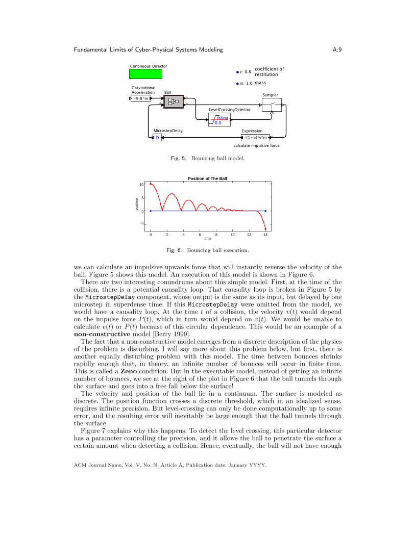
To better understand the implications of the causality relation between an impulse and theintegrated output, consider the well-studied bouncing-ball problem. Consider a ball that issubject to the constant downward force of gravity. The gravitational force is shown on theleft in Figure 5, with value −9.8m, where m is the mass. The Ball in the figure is the onein Figure 3. This force causes it to accelerate until it collides with a rigid surface.

Let’s assume a partially inelastic collision that loses some energy so that each bounce ofthe ball rises to a lesser height than the previous bounce. When it collides with the surface,

3Note that implicit numerical integration techniques introduce additional dependencies, and when usingsuch techniques, it is necessary to know (or estimate) F (t) in order to calculate v(t). This dependence, how-ever, is not present in the fundamental model from calculus nor in explicit numerical integration techniques.



Fig. 5. Bouncing ball model.

-5

0

5

10

0 2 4 6 8 10 12 14

Position of The Ball

time

posi

tion

Fig. 6. Bouncing ball execution.

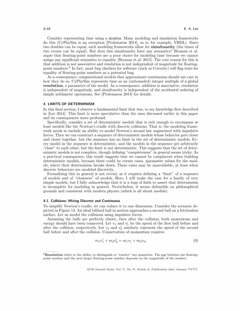
we can calculate an impulsive upwards force that will instantly reverse the velocity of theball. Figure 5 shows this model. An execution of this model is shown in Figure 6.

There are two interesting conundrums about this simple model. First, at the time of thecollision, there is a potential causality loop. That causality loop is broken in Figure 5 bythe MicrostepDelay component, whose output is the same as its input, but delayed by onemicrostep in superdense time. If this MicrostepDelay were omitted from the model, wewould have a causality loop. At the time t of a collision, the velocity v(t) would dependon the impulse force P (t), which in turn would depend on v(t). We would be unable tocalculate v(t) or P (t) because of this circular dependence. This would be an example of anon-constructive model [Berry 1999].

The fact that a non-constructive model emerges from a discrete description of the physicsof the problem is disturbing. I will say more about this problem below, but first, there isanother equally disturbing problem with this model. The time between bounces shrinksrapidly enough that, in theory, an infinite number of bounces will occur in finite time.This is called a Zeno condition. But in the executable model, instead of getting an infinitenumber of bounces, we see at the right of the plot in Figure 6 that the ball tunnels throughthe surface and goes into a free fall below the surface!

The velocity and position of the ball lie in a continuum. The surface is modeled asdiscrete. The position function crosses a discrete threshold, which in an idealized sense,requires infinite precision. But level-crossing can only be done computationally up to someerror, and the resulting error will inevitably be large enough that the ball tunnels throughthe surface.

Figure 7 explains why this happens. To detect the level crossing, this particular detectorhas a parameter controlling the precision, and it allows the ball to penetrate the surface acertain amount when detecting a collision. Hence, eventually, the ball will not have enough


A:10 E. A. Lee

-8

-6

-4

-2

0

2

4

x10-5

12.820 12.825 12.830 12.835 12.840


time

posi

tion

Fig. 7. Bouncing ball execution closeup showing tunneling.

Fig. 8. Model that is Zeno if the Collatz conjecture is false (due to Ben Lickly).

energy to rise above the surface. Any implementation that allows penetration and modelsthe surface as a discrete threshold will suffer this tunneling.

As with Newton’s cradle, we might conclude that using discrete models isn’t the rightchoice. We could construct a more detailed model of the physics, but as I’ve observed before,the resulting model may not be any more faithful, and the cost in modeling complexity canbe high. We will see below that there is an atlernative solution that further embracesdiscreteness, which is to model this system as a modal model.

Although the computational model in Figure 5 is deterministic, it is difficult to predictwhen the tunneling will occur. This will depend on the exact details of numerical compu-tation, including the precision with which real numbers are represented and the algorithmsused to perform arithmetic on them. At this point, it might be more useful to considerthe model to be nondeterministic, and not even attempt to include in the model suchcomputational details. An idealized model, one that embraces the continuum, becomes adeterministic ideal against which the nondeterministic approximations are evaluated. Thisseems to suggest a tradeoff between precision and determinism, in that higher precisioncould get us “closer” (in some sense) to the deterministic ideal. However, as I will showbelow, this line of reasoning breaks down because determinism is incomplete. Even lettingthe precision approach infinity does not solve the problem.

3.3. Detecting Zeno Behavior is Hard

The bouncing ball model above exhibits Zeno behavior, where an infinite number of eventsoccur in finite time. Any modeling framework that is sufficiently expressive to describe suchmodels will have challenges handling the models. A framework that handles all events inchronological order will either get stuck at the Zeno point or suffer from unexpected behav-ior due to quantization errors near the Zeno point (Figures 6 and 7 illustrate the latter).Techniques exist for getting past the Zeno point in practice (see for example [Zheng et al.2006]) and in theory (see [Matsikoudis and Lee 2013], which uses transfinite induction), butthese techniques are either incomplete (they fail on some models) or not (directly) computa-



Fig. 9. Modal model of the bouncing ball that does not tunnel.

tional. It would be desirable if Zeno models could be recognized and rejected to circumventsuch problems, but unfortunately, this is not possible. Figure 8 shows a model (due to BenLickly) that may or may not have Zeno behavior. Whether it has Zeno behavior depends onwhether a famous conjecture is true or false. Specifically, the Collatz conjecture states:

For any natural number n ≥ 1, if n is even, divide it by 2; if n is odd multiply itby 3 and add 1. Repeat the process indefinitely. The conjecture is that no matterwhat number you start with, you will always eventually reach 1.

This conjecture is as yet unproven true or false. If the conjecture is false, then the model inFigure 8 is a Zeno model when the input is a counterexample to the conjecture. An infinitenumber of events will circulate in the loop with spacing between them equal to 1/m2, wherem is the count of events from the input that is the counterexample. Otherwise, the modeldoes not exhibit Zeno conditions for any input. This shows definitively that detecting Zenosystems is hard.

3.4. Modal Models

One possible interpretation of the problem with the bouncing ball is that the model thatdetects a collision with the surface becomes invalid when the ball motion drops below somethreshold. Indeed, in the physical world, a ball won’t bounce an infinite number of times. Itwill stop. The model of a stopped ball is quite different from the model of a bouncing ball(and much simpler!).

Modal models (generalized hybrid systems) split models into modes, and provide a tran-sition system ensures that a mode is active only when the model in that mode is valid.A modal model for the bouncing ball is shown in Figure 9. Details of the notation in this(executable) model are given in [Ptolemaeus 2014], but for our purposes, it is enough tonotice that guarded transition moves the model from falling to sitting when the positionand velocity drop below a threshold. Interestingly, the behavior of the model is not verysensitive to the choice of this threshold, as long as the transition is taken before the balltunnels.

A plot of the new execution is shown in Figure 10. This model has more discrete elementsthan the original model, in that the guarded transitions are (semantically) instantaneous.


A:12 E. A. Lee

0

2

4

6

8

10

0 2 4 6 8 10 12 14


time

posi

tion

Fig. 10. Trajectory of the bouncing ball that does not tunnel.

Fig. 11. A model of a physical system where causality changes when modes change.

By making the model more discrete, we are also able to make it simpler. And we no longerconfront the tradeoff between determinism and precision.

3.5. Modal Causality

In this section, I study a modal model where the causality relationship between variableschanges between modes. Consider the example shown in Figure 11, which was also consid-ered in [Lee 2014; Mosterman and Biswas 1995]. This is a very practical circuit, representinga pattern that is widely used in CPS when a switch is used to turn on and off an inductiveload, such as a motor. The dashed lines abstract this circuit as two components, a controlleron the left and the load on the right. When the switch is closed, the controller supplies avoltage w and current j to the load. There are several variables in this model, currents h,j, and i, and voltages u, v, and w. To build a constructive model, we would like to identifysome of these variables as inputs and outputs of the two components.

The notion of constructive models is defined formally in [Berry 1999], but loosely a modelis constructive if its behavior can be found by a terminating procedure that changes variablesfrom unknown to known in a sequence that is based on their causal relationships; i.e., if acauses b, then a must become known before b can become known.

An inductor has memory. It has the property that current flowing through it at a time tdoes not depend on the voltage across it at time t, but rather only depends on the historyof past voltages. Specifically, for the currents and voltages in the figure,

i(t) =1

L

∫ t

0

v(τ)dτ, (5)

where L is the inductance. This assumes that the initial voltage v(0) is zero at time zero;i.e., we assume that the system starts in the off position (the switch is open) and that theinductor is storing no energy. It is a basic property of integration in calculus that i(t) in (5)does not depend on v(t) at any time t.

During normal operation of this circuit, assuming that the battery voltage u is positiveand the switch is closed, the diode will be reverse biased, meaning that no current flowsthrough it (I neglect leakage). At such times t, h(t) = 0, and consequently, j(t) = i(t).



Fig. 12. Causality relationships of the load and controller components of Figure 11. In (a) the diode isreverse biased and the switch is closed. In (b), the diode is forward biased and the switch is open.

Moreover, at all times t, v(t) = w(t). Hence, when the diode is reverse biased, the loadcomponent is defined by

j(t) =1

L

∫ t

0

w(τ)dτ, (6)

With this definition, we must consider w the input and j the output, because the environ-ment of the load component cannot arbitrarily set the current j independent of the history.Figure 12(a) shows the load component with input w and output j.

For the controller, because of the resistor, w depends on the current j that the loaddraws. Hence it is reasonable to consider j to be an input and w to be an output, as shownin Figure 12(a) The battery symbol on the far left of Figure 11 represents an ideal voltagesource producing voltage u, so the battery together with the resistor model a practicalbattery.

Notice that for the controller, the voltage w(t) depends instantaneously on the currentj(t) at time t, by Ohm’s law. There is no delay from the input j(t) to the output w(t), sothere is direct feedthrough. Put another way, we cannot know the output w(t) unless we knowthe input j(t). By contrast, for the load component, the output j(t) does not immediatelydepend on the input w(t), because of (6). Hence, that component does not have directfeedthrough. As a consequence, the feedback loop in Figure 12(a) is constructive. At anytime t, the output j(t) of the load can be determined without knowing the input w(t). Acausality loop is averted. We therefore have a constructive procedure for finding thevalues of both w(t) and j(t) at time t.

When the switch is open, the situation is very different. In this case, the current j is forcedby the switch to be identically zero. This is what a switch does. Hence, the current j is nolonger an input to the controller component. It is an output. Moreover, since the switch isopen, the controller no longer has any control over the voltage w. Therefore, that voltageis no longer an output, and can only be considered an input.4 This reversal of causality isshown in Figure 12(b).

For the load component, with the switch open, the current j has now become an input.We have already established that j cannot be an input if the diode is reverse biased. Indeed,in this circuit, when the switch is opened, the diode becomes forward biased, and currentcan flow through it. In this state, the current h through the diode is equal to i, the currentthrough the inductor. The voltage w is now determined by the diode, and hence is an outputof the load component (this voltage is a property of the diode technology, but we can assumefor our purposes an ideal diode where this voltage is zero). Figure 12(b) shows a revised

4Here, I assume that every variable must be either an input or an output. In this case, the input has noeffect, but since it cannot be an output, it must be an input.


A:14 E. A. Lee

load component, where the current j is an input (forced to zero by the controller) and thevoltage w is an output.

Figure 12(b) also averts a causality loop. For the controller, the current j, the output,does not depend on the voltage w, the input, and hence, in this mode, there is no directfeedthrough from input to output. We do not need to know w(t) at time t to determinej(t). The circuit is again constructive.

The behavior of this circuit is naturally modeled using a modal model. There are po-tentially four modes, because each of the two components has two modes. The controllercomponent has a switch that is either open or closed, and the load component has a diodethat is either forward or reverse biased. A detailed model is given in [Lee 2014]. In thatmodel, two of the four modes (switch is closed and diode is forward biased, or switch isopen and diode is reverse biased) are transient. The model spends no time in them. Suchtransitory modes are called “mythical modes” by Mosterman and Biswas [Mosterman andBiswas 1995]. In fact, in two of the four modes, the model is not constructive. It has acausality loop.

The most interesting feature of this model, however, is not the mythical modes. It is thereversal of causality when switching between modes. What is an input in one mode becomesan output in the other. Moreover, the direct feedthrough property changes. These changesin causality appear to be a direct consequence of the physics of the model.

A continuous model of this system would have to get much more detailed about thephysics, delving into the mobility of charged particles. Again, there is risk that uncertaintyabout material details of the system being modeled will undermine the fidelity of the model,resulting in a model that is no more trustworthy than the discrete model. An alternative is toreject the notion of causality altogether, something that is advocated by some philosophers.5

But rejecting the notion of causality just so that we can reject the notion of discreteness issimply too high a price to pay. This author prefers to accept discreteness.

Note that even languages that embrace acausal models, such as Modelica, go to greatlengths to convert the models to causal form, e.g. using the Pantelides algorithm [Pantelides1988]. Only when such conversion is not possible are algebraic loop solvers used, and in suchcases, considerable modeling care is required to interpret the results, since solutions maynot exist or may not be unique.

3.6. Causality Loops

In equation (6), the reader may have noticed a sleight of hand. I assumed that the initialvoltage w(0) was zero. Otherwise, the correct equation is a little bit different,

j(t) =1

L

[w(0) +

∫ τ

0

w(τ)dτ

]. (7)

Now we have a problem. At time zero, the integral is zero, so

j(0) =1

Lw(0). (8)

The current j(0) depends immediately on the voltage v(0). If the voltage is an input andthe current is an output (for the load component), then there is direct feedthrough, thoughonly at time zero. Since the controller component on the left also has direct feedthrough,the voltage w(0) depends immediately on the current i(0), we have a causality loop. If wedo not know v(0), then can’t find i(0), and if we do not know i(0), we cannot find v(0).

This problem is resolved in [Lee 2014] by ensuring that whenever we enter the mode wherethe diode is reverse biased, the voltage across the inductor gets set as an initial condition.

5See [Price and Corry 2007], which includes an essay arguing that there is no basis in physics for the notionof causality [Norton 2007]. Causality, it claims, is a human cognitive construction.



At the very start of the execution of the model, if the initial mode is such that the diodeis reverse biased, then that initial voltage is a parameter of the model. Upon subsequententries into this mode, the initial voltage is simply set equal to the voltage w in the previousmode. This setting is part of the mode transition function.

There are circuits, however, where the resolution to such transient causality loops is not soobvious (the causality loop is transient because it lasts zero time; after any infinitesimal timehas passed, there is no longer a causality loop). See [Cellier and Kofman 2006], page 582, foran example that intrinsically includes a causality loop. To support such models, CyPhySimincludes three algebraic loop solvers that can be tried [Lee et al. 2015]. However, withsuch causality loops, we have no assurance of the existence or uniqueness of a solution, soconsiderable care in modeling is required.

3.7. Representing a Continuum

Computers cannot directly deal with quantities in a continuum. Every object manipulatedby a digital computer is a member of a countable set (or strictly speaking, a finite set, sincememory is always bounded; but often the bound is so large that we can neglect the finite-ness). When modeling physical behaviors in a computer, we have to approximate the contin-uum somehow. Furia et al. state “normal numerical algorithms deal with rational numberssince they can approximate real numbers” [Furia et al. 2010]. However, rational numbersare in fact quite expensive to compute with. Representing a rational number (fully) requirestwo unbounded integers, one for the denominator, and one for the numerator. Adding tworational numbers requires finding the least common multiple of the denominators, scalingthe numerators and denominators, and then adding. If we then want to reduce each rationalnumber to a canonical form, we have to factor the numerator and denominator of the result.As a consequence, numerical algorithms that deal with rational numbers are rare indeed.

The usual approximation to real numbers in computer programs is floating-point numbersconforming to the IEEE 754 standard. The sets of float or double numbers, however, arenot dense in the reals (there are real numbers that are not limits of sequences of floating-point numbers). Moreover, these sets are in fact finite. Hence, the properties of these setsare distinctly different from the properties of real numbers, and it is not correct to simplyassume that one can arbitrarily closely approximate real numbers.

In many physical problems, it makes little sense to talk about equality of two distinctquantities in a continuum. For example, we would be on shaky ground to assert that thevoltage across two distinct capacitors is equal. Any such assertion would force our modeldown to the resolution where quantum mechanics applies, and at such scales, the assertionis prohibited.

Consider a bouncing ball model that places the position of the ball in a continuum. Ifthe position of the falling ball is continuous, then there must be instant in time (wheretime is also modeled as a continuum) when the position of the ball equals the position ofthe surface. In the idealized model using continuums, this is the instant at which the ballbounces.

Such equality is problematic in physics and even more problematic in computation. Nei-ther the position nor the time can be represented in the computer as members of a contin-uum. Hence the need for approximation. Even if the position of the falling ball is continuousin the continuum model, in any computational model, the position of the ball may progressfrom above the surface to below it without ever being equal.

But there is an even more subtle phenomenon that we cannot ignore: when we representquantities using a finite set, such as double, it is possible for two quantities to be equal. Itis essential for any modeling framework that approximates a continuum using such a finiteset to give a semantic meaning to such equality. Equality will occur sometimes. It needs tomean something. It cannot be ignored.


A:16 E. A. Lee

Consider representing time using a double. Many modeling and simulation frameworksdo this (CyPhySim is an exception [Ptolemaeus 2014], as is, for example, VHDL). Sincetwo doubles can be equal, such modeling frameworks allow for simultaneity (the times oftwo events can be equal). But does this simultaneity have any semantics? Broman et al.argue that floating-point numbers are a poor choice for modeling time because we cannotassign any significant semantics to equality [Broman et al. 2015]. The core reason for this isthat addition is not associative and resolution is not independent of magnitude for floating-point numbers.6 In fact, most bug checkers for software (such as Coverity) will flag tests forequality of floating-point numbers as a potential bug.

As a consequence, computational models that approximate continuums should use care inhow they do so. CyPhySim represents time as an (unbounded) integer multiple of a globalresolution, a parameter of the model. As a consequence, addition is associative, resolutionis independent of magnitude, and simultaneity is independent of the accidental ordering ofsimple arithmetic operations. See [Ptolemaeus 2014] for details.

4. LIMITS OF DETERMINISM

In this final section, I observe a fundamental limit that was, to my knowledge first describedin [Lee 2014]. This limit is more speculative than the ones discussed earlier in this paperand its consequences more profound.

Specifically, consider a set of deterministic models that is rich enough to encompass atleast models like the Newton’s cradle with discrete collisions. That is, the modeling frame-work needs to include an ability to model Newton’s second law augmented with impulsiveforces. Then we can construct a sequence of deterministic models whose behavior gets closerand closer together, but the sequence has no limit in the set of deterministic models. Ev-ery model in the sequence is deterministic, and the models in the sequence get arbitrarily“close” to each other, but the limit is not deterministic. This suggests that the set of deter-ministic models is not complete, though defining “completeness” in general seems tricky. Asa practical consequence, this result suggests that we cannot be complacent when buildingdeterministic models, because there could be corner cases, parameter values for the mod-els, where their determinism breaks down. These cases may be unavoidable, at least whendiscrete behaviors are modeled discretely.

Formalizing this in general is not trivial, as it requires defining a “limit” of a sequenceof models and of “closeness” of models. Here, I will make the case for a family of verysimple models, but I fully acknowledge that it is a leap of faith to assert that determinismis incomplete for modeling in general. Nevertheless, it seems defensible on philosophicalgrounds and consistent with modern physics (which is all about models).

4.1. Collisions: Mixing Discrete and Continuous

To simplify Newton’s cradle, we can reduce it to one dimension. Consider the scenario de-picted in Figure 13. An ideal billiard ball in motion approaches a second ball on a frictionlesssurface. Let us model the collisions using impulsive forces.

Assuming the balls are perfectly elastic, then after the collision, both momentum andenergy should have been conserved. Let v1 and v′1 be the speed of the first ball before andafter the collision, respectively. Let v2 and v′2 similarly represent the speed of the secondball before and after the collision. Conservation of momentum requires

m1v′1 +m2v

′2 = m1v1 +m2v2, (9)

6Resolution refers to the ability to distinguish or “resolve” two quantities. The gap between one floating-point number and the next larger floating-point number depends on the magnitude of the number.



Fig. 13. Two balls.

where m1 and m2 are the masses of the two balls, respectively. Conservation of kineticenergy requires

m1(v′1)2

2+m2(v′2)2

2=m1(v1)2

2+m2(v2)2

2. (10)

Assuming we know the starting speeds v1 and v2 and the masses, then we have two equationsand two unknowns, v′1 and v′2. This is a quadratic problem with two solutions.Solution 1: v′1 = v1, v′2 = v2 (ignore the collision).Solution 2:

v′1 =v1(m1 −m2) + 2m2v2

m1 +m2(11)

v′2 =v2(m2 −m1) + 2m1v1

m1 +m2. (12)

Note that if m1 = m2, then the two masses simply exchange velocities (as in Newton’scradle). Note further that solution 1 corresponds to tunneling, albeit for a very differentreason than in the bouncing ball example.

Now consider a more elaborate scenario, shown in Figure 14. Two (ideal) billiard ballsapproach a third stationary ball from opposite sides on a frictionless surface and collidewith the stationary ball simultaneously. How should they react?

If we consider only conservation of momentum and energy, then there is more than onepossible outcome. The conservation laws give us two equations, but there are now threeunknowns. Embracing discrete models, at the time of the collision, there are two collisions,each with two outcomes. If we reject the tunneling solutions, then it would seem that onlyone outcome remains. But it is not obvious how to combine the two non-tunneling outcomes.

A first (naive) solution, using what is known as Newton’s hypothesis, just superimposesthe resulting momentums of the two non-tunneling outcomes. If the balls all have the samemass, then the left ball will transfer its momentum to the middle ball, the right ball willalso transfer its momentum to the middle ball, and the equal and opposite momentums willcancel. All balls stop. Momentum is conserved, but not energy. This solution is shown atthe top of Figure 15. Since there is no mechanism for energy dissipation in this model, thisresolution is not satisfactory.

An alternative solution, using what is known in the literature as Poisson’s hypothesis,introduces a form of superdense time. At the time of the collision, the kinetic energy ofthe balls is instantly converted to potential energy by compressing the middle ball. Then,without time elapsing, in a second microstep, the potential energy is reconverted to kineticenergy by the middle ball expanding. But how should this ball apportion the kinetic en-ergy to the two outer balls? As it happens, if the masses of the balls are equal, there is

Fig. 14. Simultaneous collisions where one collision does not cause the other.


A:18 E. A. Lee

(a)

(b)

leftmiddle

right

02

4

6

8

10

0 1 2 3 4 5 6 7 8

Positions of Balls

time

posi

tion

leftmiddle

right

02

4

6

8

10

0 1 2 3 4 5 6 7 8

Positions of Balls

time

posi

tion

left

right

middle

middle

right

left

Fig. 15. Newton’s hypothesis vs. Poisson’s hypothesis.

only one solution, shown at the bottom of Figure 15. But if the masses are unequal, thenthere are many solutions that conserve both momentum and energy! We seem to have nobasis for picking one solution over another, so the model appears to become intrinsicallynondeterministic.

Perhaps we can resolve this conundrum by questioning the notion of simultaneity. Let’sassume that the collisions occur in some order. To embrace discreteness and leverage su-perdense time, let’s assume that no time elapses between collisions. As shown in Figure16, when the collisions occur, we arbitrarily pick one to handle, the left one in the figure,and ignore the other collision. We handle that collision, rejecting the tunneling solution.Without time elapsing, we find ourself in state (c) in the figure, where the middle and rightball are traveling towards one another and colliding. Now there is only one collision, sowe handle it in (d), leaving us in state (e). Again, without time elapsing, there is a newcollision, which we handle in (f), leaving us in state (g). After time elapses, we find ourselvesin state (h).

The balls move away at equal speed, but only if their masses are the same! If the massesare different, then the choice of which collision we handle first affects the final outcome, asdepicted in Figure 17. More than one final state conserves both momentum and energy.

Arbitrary interleaving of the collisions yields the right result (for any choice of interleav-ing), in that momentum and energy are conserved. But if the masses are not the same, evenafter excluding tunneling, there is more than one “right” result, as shown for a particularexample in Figure 17. There, three balls with masses 0.2, 1.0, and 5.0 collide simultaneously.Depending on which collision is handled first, the trajectories differ. Both shown outcomeshave the same momentum and energy after the collision as before.

Inevitably, when I present this example, someone asks me how the “real world” behaves inthis example. This is a difficult question. Recall that the Heisenberg uncertainty principlestates that we cannot simultaneously know the position and momentum of an object toarbitrary precision. But discrete modeling of these collisions depends on knowing positionand momentum precisely. Interestingly, quantum mechanics resolves this conundrum withprobabilistic models, which like our arbitrary interleaving and nondeterminism, admit morethan one behavior.



(a)

(b)

(c)

(d)

(e)

(f)

(g)

(h)

Fig. 16. One of two orderings for handling collisions.

It probably seems odd to be invoking quantum mechanics on macro-scale physics prob-lems, where Newtonian mechanics usually works just fine. But we are talking about models,and in our model, position and velocity are real numbers, and therefore have infinite pre-cision, in violation of the Heisenberg uncertainty principle. Arguably, physics tells us thatwhen the time between collisions gets small enough, our Newtonian model is no longer valid,and we need to switch to some other model.

Another way to resolve this conundrum would be to switch to a model that is moredetailed about the physics of collisions. A relatively small step in that direction, short ofmodeling localized plastic deformation, viscous damping in the material, and acoustic wavepropagation, would be to model the collisions using stiff springs at the boundaries of theballs. Such a model is deterministic, and the velocities of the balls are continuous functionsof time, but can we have confidence in the result? If we assume the stiffness of the springsis high, then the behavior exhibited by the model will be very sensitive to the time betweencollisions. Figure 18 shows multiple trajectories under this stiff-spring model where the


A:20 E. A. Lee

leftmiddle

right

-4

-2

0

2

4

0.0 0.2 0.4 0.6 0.8 1.0 1.2 1.4 1.6 1.8 2.0

Positions of Balls

time

posi

tion

leftmiddle

right

-4

-2

0

2

4

0.0 0.2 0.4 0.6 0.8 1.0 1.2 1.4 1.6 1.8 2.0

Positions of Balls

time

posi

tion

(a)

(b)

left

right

middle

middle

right

left

Fig. 17. If the masses are different, the behavior depends on which collision is handled first.

-2

-1

0

1

2

3

4

0.0 0.2 0.4 0.6 0.8 1.0 1.2 1.4 1.6 1.8 2.0

Positions of Balls

time

posi

tion

-2x10

3.990

3.995

4.000

4.005

4.010

0.0 0.5 1.0 1.5time

0.9800.985

0.990

0.995

1.000

1.005

1.010

1.00 1.01 1.02time

Fig. 18. Trajectories with a continuous, stiff-spring model where the initial position varies over a smallrange.

initial position of the right ball is varied slightly as shown in the figure. Each trajectoryis the result of a deterministic model, but the final behavior is very sensitive to the initialposition. As with chaotic models, the predictive power of this deterministic model is suspect,and may in fact be no better than the predictive power of the discrete nondeterministicmodel. Moreover, the determinism of the model could be misleading, inducing a false senseof confidence in the model.

Since the time of the collisions cannot be known precisely, we could elaborate our modelwith probabilities that quantify our uncertainty about the parameters. However, if thestiffness of the springs is high enough, these probabilistic models likely become bimodal,reflecting a temporal ordering between collisions. In this case, the probabilistic model be-comes remarkably similar to the discrete nondeterministic model, though at considerablecost in complexity.

As with all modeling exercises, we have many choices for how to model this system. Whichmodel to choose will depend on our modeling goals. Do we want a typical behavior? Theset of all possible behaviors? The set of possible behaviors weighted by probabilities? Theextreme behaviors? Any plausible behavior? This choice should be explicit. And we shouldalways choose the simplest model that meets our objectives.



Fig. 19. Non-simultaneous collisions.

4.2. Is Determinism Incomplete?

The above example has the odd property that a sequence of deterministic models “con-verges” (in some sense) to a nondeterministic one. This suggests that the set of determin-istic models is incomplete (in some sense), at least when discrete behaviors are allowed. Ageneral statement about the incompleteness of determinism is difficult to make, because theset of all models is ill defined. Also, there are many subtly different notions of completenessin mathematics. If we restrict our attention to a well-defined subset, and choose a particularnotion of completeness, then we can argue this incompleteness.

Specifically, I will study a particularly small set of well-defined models. Consider the setM of models describing one-dimensional motion of N = 3 ideal elastic balls subject toNewton’s second law, where collisions are handled with impulsive forces, and all behaviorsthat conserve momentum and energy are allowed except for tunneling. The equations ofmotion are (2) and (4). There are no external forces, so all behaviors are a consequenceof the initial conditions. We can assume that these equations are solved ideally, since theyare simple enough that given any initial condition, all eventualities can be derived in closedform. The set M includes three balls with masses m1 = 0.2, m2 = 1.0, and m3 = 5 (theseare the masses that generate the behaviors shown in Figure 17). Assume initial positionsxi(0) ∈ R, and initial velocities vi(0) ∈ R given as follows:

x1(0) = −1

v1(0) = 1

x2(0) = 0

v2(0) = 0

x3(0) = 1 + ∆

v3(0) = −1

where ∆ ∈ R is a real number. That is, there are three balls, with the two outer ones movingtowards the stationary middle one. The set M is now well defined. The only distinguishingfeature between models in M is the value of the parameter ∆. When ∆ 6= 0, the collisionswill not be simultaneous, as illustrated in Figure 19.

Following [Lee and Sangiovanni-Vincentelli 1998], we formally define a model as a set ofbehaviors. We will consider the behavior of each model over the time interval [0, 2] only,since this is sufficient for our purposes. Specifically, let B be the set of all functions of theform b: [0, 2]→ R3. For a particular model A ∈M with parameter ∆A, we say that x ∈ B isa behavior of A if for all t ∈ [0, 2], xi(t) is the position of ball i at time t, for i ∈ {1, 2, 3}.These xi are functions of time that satisfy the equations of motion and conservation laws.In words, a behavior of a model A ∈M is three functions giving the positions of the threeballs as a function of time.

A particular model A ∈M may have more than one behavior, in which case the model isnondeterministic [Lee and Sangiovanni-Vincentelli 1998]. In particular, as shown by exampleabove, there is more than one behavior that satisfies the equations of motion and conserva-tion laws when ∆A = 0. In fact, in our space of models, that is the only nondeterministicmodel.

Consider the subset D ⊂ M of deterministic models. We can define a metric on Dthat allows us to talk about models being “close.” It does not matter much which metric we


A:22 E. A. Lee

choose. To be concrete, consider two models A,A′ ∈ D. Since these models are deterministic,each has exactly one behavior. Let those behaviors be x, x′ ∈ B, respectively. We can definea distance function d as follows,

d(A,A′) =1

2

∫ 2

0

||x(t)− x′(t)||dt, (13)

where ||x|| is the L1 norm of a real vector x. It is easy to show that d is a metric.Consider a sequence of models Ai ∈ D, i ∈ {1, 2, · · ·} where

∆Ai = 1/i2.

It is easy to show that this sequence is Cauchy, which means that for any ε > 0, we canfind a positive integer N such that for all positive integers i, j > N ,

d(Ai, Aj) < ε.

However, this sequence has no limit in D, which means that the metric space D of de-terministic models is incomplete. It does not contain all its limit points. Every model inthe sequence is deterministic, and the models in the sequence get arbitrarily close to oneanother. But there is no limit that is a deterministic model.

In [Lee 2014], I show that a direct description of this scenario results in a non-constructivemodel [Berry 1999; Mendler et al. 2012] when ∆ reaches zero. To make the model construc-tive, we have to arbitrarily choose one of the possible behaviors. My formulation assumesthat this choice is handled nondeterministically. Does this assumption alone predispose theresult? For example, we could define the universe of models so that simultaneous collisionsare handled left to right, and then all models in M become deterministic. However, the aboveargument still works, because even though the above sequence of models will converge to adeterministic model, a second Cauchy sequence where

∆Ai= −1/i2

will not converge to any model in the set.Considering the collisions to be simultaneous appears to be problematic. But our set of

Newtonian models allows the left collision to occur before the right collision, and also allowsthe right collision to occur before the left. If time and space are continuums, then these twoscenarios must be able to cross one another. At the point of crossing, in this set of models,the collisions are simultaneous. To avoid this simultaneity, we need to either introduce a“hole” in the set of models (hence the incompleteness) or take more drastic measures suchas rejecting the time or space continuum. These more drastic measures amount to rejectingNewtonian physics. Hence, from principles of logic, we must either accept that determinismis incomplete or reject Newtonian physics.

An alternative is to reject discreteness. However, this does not solve the problem. Considerthe stiff-spring models illustrated in Figure 18. In this stiff-spring model, every model isdeterministic. But again, we can construct a Cauchy sequence of models of this type thatdoes not converge to a deterministic model. Just let the spring stiffness approach infinitywhile simultaneously letting the time between collisions approach zero. The same argumentsas above apply.

Generalizing this result to arbitrary sets of models and unbounded time horizons appearstreacherous. Nevertheless, the above argument shows definitively the incompleteness of de-terminism for sets of models rich enough to encompass Newton’s laws and discrete elasticcollisions. It would probably be wise to assume determinism is incomplete for any modelingframework that is rich enough to help design and understand cyber-physical systems, wherediscrete and continuous behaviors inevitably mix. As a practical matter, it means thatnondeterminism is unavoidable. I caution the reader, however, to not use this argument to



dispense with deterministic models altogether. Death is also unavoidable, but that doesn’tmean we should give up on life.

5. CONCLUSIONS

Science and engineering use models in different ways, and the differences affect the choiceof models and how they are used. For engineering, simplicity and understandability of themodels is essential for their usefulness, and the goal becomes to create physical systemsthat are faithful to the model. In science, the physical systems are given, and simplicitymay need to be sacrificed to achieve fidelity.

To achieve simplicity and understandability, clear, deterministic modeling semantics haveproven extremely valuable in the past in modeling and design of both physical systemsand cyber (computational) systems. But when these modeling frameworks are combined toengineer cyber-physical systems, determinism is usually lost. To improve this situation, weface a number of challenges. One is that widely used modeling techniques on the cyber sideabstract away time and cannot directly deal with the continuums of the physical world.Another is that widely used modeling techniques on the physical side do not deal well withdiscreteness.

Although I assert that deterministic models are useful, I am not asserting that nonde-terministic models are not useful. They are. One common use of nondeterministic modelsis to provide simpler abstractions of deterministic models. In this case, the target of thenondeterministic model is a deterministic model. If the abstraction is sound, then state-ments about the nondeterministic model are also true of the deterministic model. Sincethe nondeterministic model may be much smaller (fewer states, for example), algorithmictechniques such as model checking may be more effective.

Recognizing the differing emphasis in modeling for engineering purposes, we can make anumber of improvements in engineering practice. One is to embrace discrete behaviors, evenwhen modeling physical systems. Another is to use modal models, ensuring that a modelis used only within its regime of validity. Even with such improvements, however, there arefundamental limits that can restrict the utility of models. One is chaos, which limits theuse of models for prediction, even if the model is deterministic. Another is that discretebehaviors can introduce Zeno conditions and non-constructive models. In the latter case,models may of necessity become nondeterministic, again limiting their predictive power.And finally, we are forced to accept that any set of deterministic models rich enough tomodel Newton’s laws is incomplete, in that the set does not include all its limit points. Wewill always be faced with possible corner cases that yield nondeterministic models.

ACKNOWLEDGMENTS

I thank Eleftherios Matsikoudis for first suggesting to me that determinism might be incomplete in models

and both Matsikoudis and Gil Lederman for helpful comments on a draft of the paper. I also thank Chris

Paredis and Yaakov Bar-Shalom for suggestions that have (hopefully) improved this paper. Finally, I thankthree anonymous reviewers for very helpful comments that led to significant improvements in the paper.

Any remaining errors and opinions are entirely the responsibility of this author.

REFERENCES

Gerard Berry. 1999. The Constructive Semantics of Pure Esterel - Draft Version 3. Book Draft. http://www-sop.inria.fr/meije/esterel/doc/main-papers.html

George E. P. Box and Norman R. Draper. 1987. Empirical Model-Building and Response Surfaces. Wiley.

David Broman, Lev Greenberg, Edward A. Lee, Michael Masin, Stavros Tripakis, and Michael Wetter.2015. Requirements for Hybrid Cosimulation Standards. In Hybrid Systems: Computation and Control(HSCC).

Francois E. Cellier and Ernesto Kofman. 2006. Continuous System Simulation. Springer.


A:24 E. A. Lee

Thomas Huining Feng, Edward A. Lee, Xiaojun Liu, Christian Motika, Reinhard von Hanxleden, andHaiyang Zheng. 2014. Finite State Machines. Ptolemy.org, Berkeley, CA. http://ptolemy.org/books/Systems

Carlo A. Furia, Dino Mandrioli, Angelo Morzenti, and Matteo Rossi. 2010. Modeling Time in Computing:A Taxonomy and a Comparative Survey. Computing Surveys 42, 2 (2010), 6:1–6:59.

Solomon Wolf Golomb. 1971. Mathematical models: Uses and limitations. IEEE Transactions on ReliabilityR-20, 3 (1971), 130–131. DOI:http://dx.doi.org/10.1109/TR.1971.5216113

Gilles Kahn and D. B. MacQueen. 1977. Coroutines and Networks of Parallel Processes. In InformationProcessing, B. Gilchrist (Ed.). North-Holland Publishing Co., 993–998.

Edward A. Lee. 1999. Modeling Concurrent Real-time Processes Using Discrete Events. Annals of SoftwareEngineering 7 (1999), 25–45. DOI:http://dx.doi.org/10.1023/A:1018998524196

Edward A. Lee. 2014. Constructive Models of Discrete and Continuous Physical Phenomena. IEEE Access2, 1 (2014), 1–25. DOI:http://dx.doi.org/10.1109/ACCESS.2014.2345759

Edward A. Lee. 2015. The Past, Present, and Future of Cyber-Physical Systems: A Focus on Models. Sensors15, 3 (2015), 4837–4869. DOI:http://dx.doi.org/10.3390/s150304837

Edward A. Lee, Mehrdad Niknami, Thierry S. Nouidui, and Michael Wetter. 2015. Modeling and Simu-lating Cyber-Physical Systems using CyPhySim. In International Conference on Embedded Software(EMSOFT). ACM, Amsterdam, The Netherlands.

Edward A. Lee and Alberto Sangiovanni-Vincentelli. 1998. A Framework for Comparing Models of Computa-tion. IEEE Transactions on Computer-Aided Design of Circuits and Systems 17, 12 (1998), 1217–1229.

Edward A. Lee and Stavros Tripakis. 2010. Modal Models in Ptolemy. In 3rd International Workshop onEquation-Based Object-Oriented Modeling Languages and Tools (EOOLT), Vol. 47. Linkoping Univer-sity Electronic Press, Linkoping University, Oslo, Norway, 11–21. http://chess.eecs.berkeley.edu/pubs/700.html

Edward A. Lee and Haiyang Zheng. 2007. Leveraging Synchronous Language Principles for Heteroge-neous Modeling and Design of Embedded Systems. In EMSOFT. ACM, Salzburg, Austria, 114 – 123.DOI:http://dx.doi.org/10.1145/1289927.1289949

Eleftherios Matsikoudis and Edward A. Lee. 2013. On Fixed Points of Strictly Causal Func-tions. In International Conference on Formal Modeling and Analysis of Timed Sys-tems (FORMATS), Vol. LNCS 8053. Springer-Verlag, Buenos Aires, Argentina, 183–197.DOI:http://dx.doi.org/10.1007/978-3-642-40229-6 13

Michael Mendler, Thomas R. Shiple, and Gerard Berry. 2012. Constructive Boolean circuits and theexactness of timed ternary simulation. Formal Methods in System Design 40, 3 (2012), 283–329.DOI:http://dx.doi.org/10.1007/s10703-012-0144-6

Modelica Association. 2014. Functional Mock-up Interface for Model Exchange and Co-Simulation. ReportVersion 2.0. https://www.fmi-standard.org/downloads

Pieter J. Mosterman and Gautam Biswas. 1995. Modeling Discontinuous Behavior with Hybrid BondGraphs. In Ninth Qualitative Reasoning Workshop. Amsterdam, 139–147.

John D. Norton. 2007. Causation as Folk Science. In Causation, Physics, and the Constitution of Reality,Huw Price and Richard Corry (Eds.). Clarendon Press, Oxford, 11–44.

Martin Otter, Hilding Elmqvist, and Jose Daz Lopez. 2005. Collision Handling for the ModelicaMultiBody Library. In Modelica Conference. Hamburg, Germany, 45–53. http://elib.dlr.de/12299/1/otter2005-modelica-collision.pdf

Constantinos C. Pantelides. 1988. The Consistent Initialization of Differential-Algebraic Sys-tems. SIAM Journal of Scientific and Statistical Computing 9, 2 (1988), 213–231.DOI:http://dx.doi.org/10.1137/0909014

Huw Price and Richard Corry (Eds.). 2007. Causation, Physics, and the Constitution of Reality. ClarendonPress, Oxford.

Claudius Ptolemaeus (Ed.). 2014. System Design, Modeling, and Simulation using Ptolemy II. Ptolemy.org,Berkeley, CA. http://ptolemy.org/books/Systems

David E. Stewart. 2000. Rigid-Body Dynamics with Friction and Impact. SIAM Rev. 42, 1 (2000), 3–39.DOI:http://dx.doi.org/10.1137/S0036144599360110

Lothar Thiele and Pratyush Kumar. 2015. Can Real-Time Systems be Chaotic?. In EMSOFT. ACM, Am-sterdam, The Netherlands, 21–30.

Michael M. Tiller. 2001. Introduction to Physical Modeling with Modelica. Kluwer Academic Publishers.

Haiyang Zheng, Edward A. Lee, and Aaron D. Ames. 2006. Beyond Zeno: Get on with It!. In HybridSystems, Computation, and Control (HSCC), J Hespanha and A. Tiwari (Eds.), Vol. LNCS 3927.Springer-Verlag, 568–582. DOI:http://dx.doi.org/10.1007/11730637 42


a fundamental limits of cyber-physical systems … · equations that describe the semiconductor...

Documents