a fundamental comparison of international real estate...

Introduction

This study extends the earlier analysis of Pagliari and Webb (1992) of U.S. commercialreal estate returns to returns in Australia, Canada and the United Kingdom, as well asthe United States, for the period 1985–95. As in that earlier study, total returns areunbundled into their fundamental components: initial yield, income growth and shifts incapitalization rates. For analytical convenience, this study takes the perspective of a U.S.-based investor1 who invests internationally. Therefore, the “foreign” currencies areadjusted by the then-prevailing foreign exchange rate to the equivalent U.S. dollaramount. The path of these currency-adjusted components of return are then examinedover the relevant time period. Additionally, this study separately examines the office,retail and warehouse sectors in each country. Without this property-type disaggregation,spurious cross-country comparisons can result due to the varying mix of propertiescontained in each country’s composite index.2

JOURNAL OF REAL ESTATE RESEARCH 1

317

Joseph L. Pagliari, Jr.*James R. Webb**

Todd A. Canter***Frederich Lieblich****

A Fundamental Comparison of International Real Estate Returns

*Citadel Realty, Inc., 2700 River Road, Suite 106, Des Plaines, Illinois 60018.**Real Estate Research Center, College of Business, Cleveland State University, 1860 E. 18th Street, Cleveland,Ohio 44114.***LaSalle Partners Limited, 200 East Randolph Drive, Chicago, Illinois 60601****SSR Realty Advisors, One North Broadway, White Plains, New York 10601.Date Revised—February 1998; Accepted—February 1998.

Abstract. This study analyzes commercial real estate returns in Australia, Canada, theUnited Kingdom and the United States over the period 1985–95, from the perspective of aU.S. investor. Because national indices can consist of differing property mixes, this studyseparately analyzes the office, retail and warehouse sectors. Moreover, these analyses alsoconvert total returns into their fundamental components: initial yield, growth in income andshifts in capitalization rates. The paths of currency-adjusted income and asset values and,therefore, capitalization rates are also presented. Generally speaking, the fundamentalcomponents of retail returns across the four countries exhibit greater divergence than theoffice and warehouse sectors. It is interesting that the U.S. property sectors showed theworst performance, while the Australian retail and the British office and warehouse sectorswere the best performers (both before and after currency adjustments). Additionally, thecurrency-adjusted Australian returns were adversely effected by exchange rate movements,while the British returns were positively effected. Lastly, the correlation of the quarterlypercentage change in income was generally lower and less statistically significant than thecorrelation patterns observed among the other components of return. This might suggestthat more idiosyncratic risk can be found in the real estate space markets (as proxied byincome changes) than in the real estate capital markets (as proxied by the pricing of theincome—that is, capitalization rates), which appear to be more globally influenced.

The balance of the study is structured as follows: Section two reviews the relevantliterature. Section three describes the underlying methodology and data used to preparethe analyses described above. Section four presents the results of these analyses. Andsection five presents our conclusions and discusses future research applications.

Literature Review

Much of the previous literature on international real estate returns has examined thediversification benefits of securitized real estate returns. For example, Mull and Soenen(1997), using dollar-denominated returns, found that the inclusion of U.S. real estateinvestment trusts (REITs) in mixed-asset, foreign portfolios did not significantly increaserisk-adjusted returns over the 1985–94 time period. In contrast, Eichholtz (1996), usinglocal-currency-based returns (which, therefore, reflect a perfectly hedged currencyexposure), found significantly lower correlations between cross-country real estate returnsthan between stock or bond returns and, therefore, asserts that intentional diversificationimproves the efficiency of the real estate portfolio more so than for stocks or bonds. Morerecently, Eichholtz (1997) expands his analysis, by increasing the number of countriescovered and by reporting dollar-denominated returns, as well as local-currency returns,and finds that the correlation between real estate securities and common stock returnsvaries greatly by country. Along similar lines, Asabere, Klieman and McGowan, Jr. (1991)examined the risk/return attributes of international (securitized) real estate equities overthe 1980–88 time period. They found, using dollar-denominated returns, that inter-national real estate equities offered higher returns—but at higher risk levels—than didU.S.-based REITs and that the two series were weakly, but positively, correlated. Newelland Webb (1996) also assessed the risk of international real estate investments. However,they used unsecuritized real estate returns that required a de-smoothing adjustment (seebelow) of the appraisal-based real estate returns in order to facilitate comparisons tostock and bond returns. They found, using dollar-denominated returns, that internationalinvestors achieved improved portfolio diversification when including real estate.

The comparisons of unsecuritized real estate to securitized stock and bond investmentsis clouded by appraisal smoothing (see Geltner, 1989, 1991) as well as the lack of reliable,appraisal-based (unsecuritized) real estate data in many of the developed countries (e.g.,France and Germany). One approach to this dilemma is that of Quan and Titman (1997),who examined the relationship between (dollar-denominated) stock returns and changesin property values and in rents for seventeen countries for the period 1987–94. Usingpooled data, they found a strong statistical relationship; however, the “four countrieswith the most reliable data (the United States, Australia, Canada and Hong Kong) allshowed insignificant relations between stock and real estate prices.” Another approach isto examine the price discovery process between securitized and unsecuritized real estateequities. In the case of Barkham and Geltner (1995), they found that pricing informationin the securitized America and British property markets leads their unsecuritizedcounterparts by a year or more, when examined over the 1969–92 time period. Eichholtzand Hartzell (1996) prepared a similar study that included Canadian real estate andextended the comparison to include a common stock index for each country. They foundthat securitized real estate was closely correlated with the stock market and predicted (orled) appraisal-based indices.

318 JOURNAL OF REAL ESTATE RESEARCH

VOLUME 13, NUMBER 3, 1997

Other research has concentrated on the diversification benefits of foreign, un-securitized real estate investment. The results have been mixed. For example, Ziobrowskiand Curcio (1991) examine the potential benefits of adding U.S. real estate to theportfolios of British and Japanese investors. They suggest that exchange rate volatilityoffsets any potential diversification benefits to foreign investors for the 1973–87 timeperiod. More narrowly, Hudson-Wilson and Stimpson (1996) examined the case for theinclusion of U.S. real estate in Canadian property portfolios. While they too find currencyrisk to be substantial, their results suggest that Canadian investors would have benefitedby including U.S. real estate for the 1980–94 time period.

However, little of the previous research has focused on the fundamental factors(capitalization rates, earnings growth, etc.) of returns and how they compare acrossinternational property sectors. This is a somewhat curious development since mostportfolio optimization procedures rely on the use of historical return patterns to generatethe return and covariance estimates needed to optimize portfolio selection. And, asJorion (1992) observed, these estimates are observed with error and, therefore, introduceestimation risk into the optimization process. Given the rigid nature of the optimizationprocess, this risk can produce large errors when compared to the “true” optimal port-folio. This problem is compounded by the tension between requiring a sufficiently long-time series such that the true pattern of returns emerges and acknowledging that theunderlying distribution of returns may not be stable. The fundamental factors of returncan provide important insights into this situation.

Data and Methodology

This section describes both the data and the underlying methodology used to generatethe results of the analyses contained in this study. First, the data consists of income-producing, commercial properties in Australia, Canada, the United Kingdom, and theUnited States. To increase comparability, all four data series are treated as beginning in 1985, though in some cases the underlying data series began earlier. Exhibit 1summarizes certain important characteristics of each data series. Thereafter, each seriesis briefly described.

FUNDAMENTAL COMPARISON OF INTERNATIONAL RE RETURNS 319

Exhibit 1

Summary Characteristics for Data Series

Country Data Provider Start Date Reporting Frequency

Australia BOMA of Australia Limited* 1985 Semiannually

Canada Frank Russell Company 1985 Quarterly

United Kingdom Investment Property Databank 1987 Monthly **

United States NCREIF 1978 Quarterly

* In 1996, the name was changed to Property Counsel of Australia.** An annual return series began in 1971, while the monthly series began in 1987. For purposes

of these analyses, the annual returns for 1985 and 1986 were converted to quarterly equivalents.

AustraliaThe Building Owners and Managers Association (BOMA), in conjunction withthe Frank Russell Company, publishes performance data (income, appreciationand total returns) for institutional-grade Australian real estate. The index ispublished semiannually, available from December 1984. In addition to thecomposite index, indices for CBD-office, retail and industrial properties areavailable. As of December 31, 1995, the composite index comprised 583properties with a total market value of $(Australian) 32.7 billion3 (or, $(U.S.)24.3 billion).

CanadaThe Russell organization publishes performance data for institutional-gradeCanadian real estate. The index is published quarterly, available from 1985. Inaddition to the composite index, indices for apartments, hotel, industrial,mixed-use, office, and retail properties are available. However, this studyanalyzes only the office, retail and warehouse sectors. As of December 31, 1995,the composite index comprised 1,118 properties with a total market value of$(Canadian) 15.3 billion (or, $(U.S.) 11.2 billion).

United KingdomThe Investment Property Databank (IPD) publishes two sets of performancedata for institutional-grade real estate in the United Kingdom: 1) the Long-Term Index reports annually since 1971, and 2) the Monthly Index reportsmonthly performance since 1987. In addition to the composite index, indicesare also available for office, retail and industrial properties. As of December 31,1995, the composite index comprised 1,924 properties with a total market valueof £5.0 billion4 (or, $(U.S.)7.8 billion).

United StatesThe NCREIF organization5 publishes performance data for institutional-gradereal estate in the United States. The index is published quarterly, available from 1978. In addition to the composite index, indices for apartment, office,retail, R&D/office and warehouse properties are available. However, this studywill examine only the composite, office, retail, and warehouse indices. As ofDecember 31, 1995, the composite index comprised 2,318 properties with atotal market value of $(U.S.) 47.6 billion.

More detailed descriptions of these data can be found in Gordon (1991) and Newelland Webb (1994).

While the methodology for unbundling total returns into their fundamental com-ponents (initial yields, growth in income and shifts in capitalization rates) is more fullydescribed in Pagliari and Webb (1992) and Pagliari and Webb (1995), the essence of theprocess can be characterized as using the reported income and appreciation returns tosuccessively generate imputed income and property values, from which the fundamentalcomponents of return can be determined. Additionally, the data providers for theAustralian and British real estate returns have methodologies for calculating income andappreciation returns that differ from one another as well as from the methodology used



to create the Canadian and American real estate returns. A summary of the ways inwhich the various data sets are used to create the imputed income and property values ispresented in the Appendix.

As noted earlier, it is imperative to restate the foreign-currency-denominated returns intothe domestic currency. Accordingly, the U.S.-dollar equivalents of the Australian dollar,the British pound and the Canadian dollar over the 1985–95 time period are presented inExhibit 2. The data underlying Exhibit 2 show that only the British pound is converted tothe U.S. dollar at more than one-for-one, while the Australian and Canadian dollars areconverted at a rate of less than one U.S. dollar. Moreover the volatility of the foreignexchange rates also impacts the path of currency-adjusted income and property values.

Perhaps more interesting is that the right half of Exhibit 2 also displays the summarystatistics related to the percentage change in quarterly foreign exchange rates. Whenviewed from the perspective of their percentage change, foreign exchange rates display theclassical, near-zero mean-reverting pattern associated with a “random walk.” See Black(1995) and Kritzman (1989) for discussions of central bank-induced distortions incurrency returns.6 However, as noted subsequently, there are subperiods of persistentpositive and negative exchange rate returns which, in turn, directly impact the U.S.investor owning foreign real estate.

Results

We apply the methodology to the data described above for the three property types(office, retail and warehouse) for each of the four countries (Australia, Canada, theUnited Kingdom, and the United States).

The International Office Sector

As noted above and using the U.S. total index as a template, each of the three majorproperty types (office, retail and warehouse) will be analyzed from an internationalperspective, beginning with the office sector. The analysis will take a slightly different tactfrom above: rather than simultaneously analyzing the fundamental components of return(income, asset values and capitalization rates) for one country, each component will be


Exhibit 2

Quarterly Exchange Rates (and Their Percentage Change)

Stated in Terms of the U.S. Dollar for the Period 1985–95

Quarterly Percentage Change inExchange Rates Quarterly Exchange Rates

United UnitedAustralia Canada Kingdom Australia Canada Kingdom

Avg. 0.7347 0.7857 1.6125 -0.0014 -0.0005 0.0078

Std Dev. 0.0502 0.0566 0.1662 0.0517 0.0211 0.0586

analyzed individually, but simultaneously, for all four countries. The analysis begins withExhibit 3 displaying the quarterly, currency-adjusted net operating income generated bya $100 (U.S.) investment in each of the four countries’ office sectors.

As can be seen from Exhibit 3, U.S. office income appears to consistently declinethroughout most of the analysis period. However, for Australia, Canada and the UnitedKingdom, income continues to rise into the early 1990s, after which there is a pro-nounced decline, such that the ending (1995:4) income for Australia and Canadaapproaches that of the U.S. (i.e., ending values of $1.75 and $1.32 for the Australian andCanadian series, while the corresponding U.S. value is $1.02). The British income seriesremains at a level (i.e., an ending value of $3.18) substantially higher than the othercountries; however, as noted subsequently, much of this growth is attributable tofavorable pound/dollar exchange-rate fluctuations. Though not readily apparent from thedata presented in Exhibit 2, the peak and subsequent trough of the Australian, Canadianand the United Kingdom office income series follows the same trend observed in the U.S.series when viewed over the entire length of the 1978–95 time period.7 The relationship ofthe Canadian and U.S. data series is interesting given the geographic proximity and theinterconnectedness of their economies. None of the other potential two-countrycombinations offer the same degree of proximity and connectedness. That said, theAustralian and Canadian office time series of income levels displays a near one-to-onecorrespondence.

Exhibit 4 depicts the path of office property values over the 1985–95 time period. Whilethe path of property values is smoother8 than observed for the path of income values (seeExhibit 6), much the same trends are observed.

As can be seen from Exhibit 4, the decline in U.S. office property values appearsconsistent throughout the analysis. As above, the Canadian office property valuescontinue to rise until 1991, after which there is a pronounced decline, such that the



Exhibit 3

The Office Sector Comparison of Quarterly, Currency-Adjusted Income

5.00

4.00

3.00

2.00

1.00

0.00

Qu

arte

rly

Inco

me

for

$100

(U

.S.)

Inve

stm

ent

($)

1985 1986 1987 1988 1989 1990 1991 1992 1993 1994 1995

Australia Canada United Kingdom United States

ending (1995:4) property value approaches that of the U.S. (i.e., ending value of $69.88for the Canadian series, while the corresponding U.S. value is $44.97). As before andthough not readily apparent from the data presented in Exhibit 4, the peak andsubsequent trough of the Canadian office income series follows the same trend observedin the U.S. series when viewed over the entire length of the 1978–95 time period. For bothseries, the decline in asset value is astounding. With an initial investment of $100 (U.S.),the average U.S. office property value fell by approximately 56% over the 1985–95 timeperiod, while the Canadian series witnessed a near-identical percentage decline (i.e., 53%)from its maximum property value (of nearly $150, reached in 1990). For the Australianand British paths of property values, the rise-and-fall pattern is equally pronounced;however, the ending values are greater than the initial (1985) investment of $100. In thecase of the Australian office market, property values plummeted to an ending value of$103 from a peak value of $200—a decline of approximately 48%. Meanwhile, in the caseof the British office market, property values fell to an ending value of $149 from a peakvalue of $252—a decline of approximately 41%.

Exhibit 5 depicts the path of capitalization rates for office properties over the 1985–95time period. The capitalization rates were computed using the past four quarters oftrailing earnings. This computation was deemed better than alternative approaches forthree reasons: (a) the use of four quarters mitigates the seasonality and volatility associ-ated with quarterly earnings; (b) the use of trailing earnings allows the capitalization rateseries to be constructed with the most recent data; and (c) trailing earnings are availableand consistent to most all market participants, whereas forecasted earnings can vary byas many as the number of market participants.

While the Australian series has diverged from the other three countries in the last twoyears, there is a remarkable consistency in the capitalization rates for office propertyvalues for all four countries. We find it interesting that this might suggest greater


1985 1986 1987 1988 1989 1990 1991 1992 1993 1994 1995

Exhibit 4

The Office Sector Comparison of Quarterly, Currency-Adjusted Asset Value

300

250

200

150

100

50

0

Qua

rter

ly A

sset

Val

ues

for

$100

(U

.S.)

Inve

stm

ent

($)

1985 1986 1987 1988 1989 1990 1991 1992 1993 1994 1995


integration of international capital markets and substantially less integration of localspace-market conditions. That is, the pricing of properties (as proxied by theircapitalization rates) is globally influenced (if not determined) while space-marketconditions (as proxied by the income series) are locally influenced (if not determined).These empirical results are consistent with much of the theory surrounding theidiosyncratic behavior of real estate space markets.

Because the scale of a graph can obscure the values of the underlying data, Exhibit 6was prepared to provide summary statistics on the components of return, as well as totalreturn. As can be observed in this exhibit, the U.S. office sector displayed the lowestquarterly currency-adjusted total return along with the lowest standard deviation ofreturn (see Panel A). The United Kingdom generated the highest return, but Australiahad the most volatility. The returns of all four countries were positively and significantlycorrelated. But more fundamentally, what gives rise to these patterns of return andvolatility? The balance of Exhibit 6 and Exhibit 7 are intended to illuminate thesepatterns.

The Canadian income series had a near-zero growth rate (with the most volatilityhowever), while the U.S. office sector experienced nearly a 1% quarterly decrease inincome and the U.K. experienced nearly a 2% quarterly increase in income (see Panel B).Similarly, the American series of office values (see Panel C) experienced a quarterlydecline that was also approximately 100 basis points lower than the Canadian series (i.e.,-1.78% v. -0.72%) while the Australian and British office markets experienced substantialincrease in quarterly property values. Note that less than 30 basis points separate theaverage Canadian, British and American capitalization rates (see Panel D) over the1985–95 time period, while the Australian office sector’s average capitalization rate wasconsiderably lower than the other three countries. The U.K. and U.S. series had highervolatilities, which is interesting since the U.S. income and asset value (office) series



Exhibit 5

The Office Sector Comparison of Rolling Four-Quarter Capitalization Rates

12.0

10.0

8.0

6.0

4.0Ro

llin

g F

ou

r-Q

uar

ter

Cap

Rat

es (

%)

1985 1986 1987 1988 1989 1990 1991 1992 1993 1994 1995



Exhibit 6

Summary Statistics for the Office Sector

Quarterly Currency-Adjusted Total Returns for the Period 1985–1995

Panel A: Total Returns:

Risk Return Parameters Correlation Matrix (with Associated p-values)

Arithmetic Std Dev. United UnitedCountry Mean (%) (%) Country Australia Canada Kingdom States

Australia 1.96 7.09 Australia 100.0 53.9% 55.5% 38.0%p = .000 p = .000 p = .000

Canada 1.11 4.40 Canada 53.9% 100.0% 49.7% 42.6%p = .000 p = .001 p = .004

United Kingdom 2.96 6.93 United Kingdom 55.5% 49.7% 100.0% 26.8%p = .000 p = .001 p = .079

United States 0.01 2.23 United States 38.0% 42.6% 26.8% 100.0%p = .011 p = .004 p = .079

Panel B: Percentage Change in Quarterly Income Amounts:







Panel C: Percentage Change in Quarterly Asset Values:







generated the least volatility. Lastly, each of the fundamental “pricing” components (i.e.,the percentage change in asset values and the level of capitalization rates) showed positiveand significant9 correlations across countries (see Panels C and D), while the incomecomponents (see Panel B) are generally lower and less statistically significant. Theseempirical results may corroborate the earlier assertion regarding the pricing of propertiesas more globally influenced and the space-market conditions as more locally influenced.

The data displayed in Exhibits 3–6 can also be used to restate each country’s totalreturn from office investments in terms of their underlying fundamental components ofreturn. See Exhibit 7.

Additionally, Panels A–C also identify the currency returns10 associated with a foreigninvestment by a U.S.-based real estate investor, the most profound of which is found inrelation to the British property market (Panel C: an average currency return of 2.46% perannum).11 Conversely, the Australian property market suffered the most dramatic lossdue to currency returns (Panel A: an average currency return of 21.11% per annum).12

In a pattern to be repeated for the other two property types, the U.S. office sector (seePanel D) was the worst performing of the four countries examined here. Its poorperformance can be tied directly to the persistent negative earnings growth (whichaveraged 24.32% per annum) and, not surprisingly, a corresponding rise in capitalizationrate (the effect of which was to reduce total returns by -1.78% per annum). In this regard,Canada’s pattern of returns (see Panel B) most closely resembled that of the U.S.However, the magnitude of these problems was less dramatic for the Canadian properties.Conversely, the Australian (Panel A) and British (Panel C) office markets actuallygenerated positive earnings growth. While all countries witnessed an increase incapitalization rates, the increase was most pronounced in the British and American officemarkets.

The International Retail Sector

Like the office sector analysis above, this section individually analyzes each of the



Exhibit 6 (continued)

Panel D: Rolling Four-Quarter Capitalization Rates:








Exhibit 7

Office Index: Annualized Return Attributes from 1985:1–1995:4

1985–88 1989–92 1993–95 1985–95(4 Yrs) (4 Yrs) (3 Yrs) (11 Yrs)

(%) (%) (%) (%)

Panel A: Australia

Real Estate Return in Domestic Currency:

Initial Yield 6.62 5.79 7.19 6.62

Growth in Income 15.35 23.84 25.67 1.70

Change in Cap Rate* 2.59 24.38 2.25 20.20——— ——— ——— ———

Estimated Return 24.55 22.43 3.77 8.11

Real Estate-related Timing/Methodology Differences 0.37 21.75 1.15 0.15——— ——— ——— ———

Time-weighted Return—Domestic Currency 24.92 24.18 4.92 8.26——— ——— ——— —————— ——— ——— ———

Currency-Adjusted Real Estate Return (U.S. Investor):

Real Estate Return in Domestic Currency 24.92 24.18 4.92 8.26

Currency Returns 0.51 24.14 1.62 21.11

Currency Returns’ Related Joint Effects 20.13 20.17 20.08 0.09——— ——— ——— ———

Time-weighted Return—Currency-adjusted U.S. 25.56 28.15 6.62 7.06——— ——— ——— —————— ——— ——— ———

*Capitalization Rates:

Going-in Rate 6.57 5.97 7.31 6.57

Going-out Rate 5.97 7.31 6.79 6.79

Panel B: Canada


Initial Yield 6.52 7.12 6.96 6.52

Growth in Income 7.04 25.23 28.38 21.26











Going-in Rate 6.52 7.01 6.72 6.52

Going-out Rate 7.01 6.72 7.89 7.89

fundamental components of return (income, asset values and capitalization rates)simultaneously for all four countries. The analysis begins with Exhibit 8 displaying thequarterly, currency-adjusted income generated by a $100 (U.S.) investment in each of thefour countries’ retail sectors.

As can be seen from Exhibit 8, retail income in Australia, the U.K. and the U.S.




1985–88 1989–92 1993–95 1085–95(4 Yrs) (4 Yrs) (3 Yrs) (11 Yrs)

(%) (%) (%) (%)

Panel C: United Kingdom


Initial Yield 6.20 5.40 10.04 6.20

Growth in Income 6.58 8.26 24.81 4.29











Going-in Rate 6.08 5.15 10.01 6.08

Going-out Rate 5.15 10.01 8.56 8.56

Panel D: United States


Initial Yield 6.64 6.41 8.46 6.64

Growth in Income 23.73 24.71 24.57 24.32



Timing/Methodology Differences 20.01 20.78 20.21 20.62——— ——— ——— ———

Time-weighted Return 4.27 25.21 1.29 0.07——— ——— ——— —————— ——— ——— ———


Going-in Rate 6.71 6.30 8.38 6.71

Going-out Rate 6.30 8.38 9.09 9.09

appears fairly consistent—as compared to the office sector—throughout the analysisperiod. For Canada, on the other hand, income continues to rise until 1991, after which,there is a fairly pronounced decline. Ending (1995:4) income values for Canada and theUnited Kingdom approach that of the U.S. (i.e., ending value of approximately $2.00).Exhibit 9 depicts the path of retail property values over the 1985–95 time period.

As can be seen from Exhibit 9, U.S. retail property values continued to rise until 1991,


Exhibit 8

The Retail Sector Comparison of Quarterly, Currency-Adjusted Income

4.00

3.00

2.00

1.00

0.00

Qu

arte

rly

Inco

me

for

$100

(U

.S.)

Inve

stm

ent

($)

1985 1986 1987 1988 1989 1990 1991 1992 1993 1994 1995

Exhibit 9

The Retail Sector Comparison of Quarterly, Currency-Adjusted Asset Value

180

160

140

120

100

80

60

Qua

rter

ly A

sset

Val

ues

for

$100

(U

.S.)

Inve

stm

ent

($)

1985 1986 1987 1988 1989 1990 1991 1992 1993 1994 1995



after which, they fell below their initial 1985 levels. Canadian retail property values alsocontinue to rise until 1991, after which there is a pronounced decline—such that theending (1995:4) property values approach those of the U.S. (i.e., ending value of $113.96for the Canadian series, while the corresponding U.S. value is $96.16).13 However, thedecline in ending values was about $45–$50 less than that observed for the office sector.Unlike the office sector, there was much greater synchronicity between the rise and fall ofCanadian and U.S. retail property values. It is interesting, too, that the Australian retailsector experienced a substantial decline in the mid- to late-1980s only to emerge as thehighest ending asset value of all four countries. While the British retail sector experienceda similar initial decline, it underperformed all other countries in all but the last coupleyears.

Exhibit 10 depicts the path of capitalization rates for retail properties over the 1985–95time period. As noted earlier, the capitalization rates were computed using the past fourquarters of trailing earnings.

As can be seen from Exhibit 10, the general pattern of capitalization rates is widelydivergent through 1991. We find it interesting that this gap narrowed considerably as thetime period progressed, such that ending capitalization rates were nearly identical for allfour countries. Like the office sector (but perhaps not to the same degree), the retailcapitalization rates suggest increasingly greater integration of international capitalmarkets and substantially less integration of local space-market conditions.

Exhibit 11 provides summary statistics on the components of return, as well as totalreturns.

As with the office sector returns, the retail sector returns are positively and significantlycorrelated across all four countries. Here too in the retail sector, the U.S. shows the lowestreturn and risk over the 1985–95 time period (see Panel A). The U.S., not surprisingly,



Exhibit 10

The Retail Sector Comparison of Rolling Four-Quarter Capitalization Rates

10.0

8.0

6.0

4.0Ro

llin

g F

ou

r-Q

uar

ter

Cap

Rat

es (

%)

1985 1986 1987 1988 1989 1990 1991 1992 1993 1994 1995



Exhibit 11

Summary Statistics for the Retail Sector























also had the lowest quarterly earnings growth (0.14%), while the Australian retail marketshowed the highest (1.32%) (see Panel B). The percentage change in quarterly UnitedKingdom retail earnings is lowly to negatively correlated with the other countries.However, two of these three correlations cannot significantly reject the null hypothesis(Ho: r50). The correlation coefficients among the remaining three countries are generallypositive but statistically insignificant, which effectively implies that the four spacemarkets act independently of one another. As with earnings, the Australian retail assetvalues (see Panel C) showed the highest quarterly growth (0.96%) and the U.S., the lowest(20.08%). As for capitalization rates (see Panel D), Australia had the highest average(which helps explain why it had the highest total return) and Britain had the lowest(6.05%), while the correlation coefficients for two of the three U.S. capitalization rateseries could not reject the null hypothesis. Note that the significant spread in averagecapitalization rates over the 1985–95 time period reflects more their initial disparity thanit does their converging ending values. While the Australian, Canadian and Americanseries reflected about the same volatility (see Panel D), the British capitalization rateseries was substantially more volatile.

The data displayed in Exhibits 8–11 can also be used to restate each country’s totalreturn from retail investments in terms of their underlying fundamental components ofreturn. See Exhibit 12.

As can be seen from Exhibit 12, the Australian retail sector (Panel A) consistentlyoutperformed its counterparts in terms of total returns. This was true in each of thesmaller time periods (with one exception, the 1993–95 period vis-à-vis the UnitedKingdom), as well as the overall eleven-year time period—even though U.S. investors inAustralian real estate suffered adverse foreign currency fluctuations. The differences inreturns for the Australian retail sector can be traced to the highest initial yield (i.e.,9.68%), the second highest income growth rate (4.13%—only the U.K. performed better)and the most favorable shift in capitalization rates. The reasons for the poor U.S.performance are abundant (see Panel D): the second lowest initial yield, the lowestincome growth and an adverse shift in capitalization rates. Meanwhile, the British retail












Exhibit 12

Retail Index: Annualized Return Attributes from 1985:1–1995:4

1985–88 1989–92 1993–95 1985–95(4 Yrs) (4 Yrs) (3 Yrs) (11 Yrs)

(%) (%) (%) (%)

Panel A: Australia


Initial Yield 9.68 8.27 8.02 9.68

Growth in Income 8.06 3.32 3.55 4.13











Going-in Rate 9.55 8.75 8.16 9.55

Going-out Rate 8.75 8.16 8.01 8.01

Panel B: Canada


Initial Yield 8.66 7.99 7.63 8.66

Growth in Income 4.17 20.32 1.32 0.93











Going-in Rate 8.62 8.05 8.18 8.62

Going-out Rate 8.05 8.18 8.12 8.12

sector (Panel C) suffered the most adverse shift in capitalization rates and the lowestinitial yield, but enjoyed the highest earnings growth rate and the highest return due tocurrency fluctuations. Lastly, Canada (Panel B) was “middle of the pack” in allcategories.




1985–88 1989–92 1993–95 1985–95(4 Yrs) (4 Yrs) (3 Yrs) (11 Yrs)

(%) (%) (%) (%)



Initial Yield 5.40 4.72 7.96 5.40

Growth in Income 5.56 10.44 1.66 6.39











Going-in Rate 5.34 4.52 7.95 5.34

Going-out Rate 4.52 7.95 7.33 7.33



Initial Yield 7.83 6.64 7.24 7.83

Growth in Income 1.14 21.90 1.39 0.09






Going-in Rate 7.82 6.85 7.27 7.82

Going-out Rate 6.85 7.27 8.23 8.23

The International Warehouse Sector

This section also individually analyzes each of the fundamental components of return(income, asset values and capitalization rates) simultaneously for all four countries. Theanalysis begins with Exhibit 13 displaying the quarterly, currency-adjusted incomegenerated by a $100 (U.S.) investment in each of the four countrie’s warehouse sector.


Exhibit 13

The Warehouse Sector Comparison of Quarterly, Currency-Adjusted Income

6.00

5.00

4.00

3.00

2.00

1.00

Qu

arte

rly

Inco

me

for

$100

(U

.S.)

Inve

stm

ent

($)

1985 1986 1987 1988 1989 1990 1991 1992 1993 1994 1995

Exhibit 14

The Warehouse Sector Comparison of Quarterly, Currency-Adjusted Asset Value

250

200

150

100

50

Qua

rter

ly A

sset

Val

ues

for

$100

(U

.S.)

Inve

stm

ent

($)

1985 1986 1987 1988 1989 1990 1991 1992 1993 1994 1995



As can be seen from Exhibit 13, the warehouse income shows a fairly steady climbthroughout the analysis period, unlike the office and retail sectors (see Exhibits 3 and 8).For Australia and Canada, income shows the familiar pattern of rising until 1991 afterwhich there is a decline. As noted earlier, the British series benefits from favorableexchange rate fluctuations as well as positive earnings growth denominated in the localcurrency, which results in a much higher ending value (i.e., $4.36 for Britain, while theAustralian, Canadian and American ending values were $2.41, $2.20 and $2.85,respectively).

Exhibit 14 depicts the path of warehouse property values over the 1985–95 time period.Again, the path of property values is generally smoother than observed for the path ofincome values (see Exhibit 13). However, the trends are quite interesting.

As can be seen from Exhibit 14, the U.S. warehouse property values continue to riseconsistently throughout the analysis (as was also generally true for their path ofearnings—see Exhibit 13). This is also the first observation of steadily increasingproperty values for any of the three U.S. property types examined here. As with the officeand retail sectors, the Australian, Canadian and British warehouse property valuescontinue to rise until 1991, after which there is a pronounced decline, such that ending(1995:4) Australian and Canadian property values fall dramatically below that of the U.S.(i.e., ending values of $93.71 and $99.38 for the Australian and Canadian series, with thecorresponding U.S. value of $160.98) while the ending British value ($176.07) remainsslightly above the U.S. value.

Exhibit 15 depicts the path of capitalization rates for industrial properties over the1985–95 time period. Here too, the trends are different from earlier observations for theoffice and retail sectors.

As can be seen from Exhibit 15, there is a remarkable constancy in the capitalizationrate series for the U.S. warehouse sector. In addition, there is a remarkable consistency in



Exhibit 15

The Warehouse Sector Comparison of Rolling Four-Quarter Capitalization Rates

12.0

11.0

10.0

9.0

8.0

7.0

6.0

5.0Ro

llin

g F

ou

r-Q

uar

ter

Cap

Rat

es (

%)

1985 1986 1987 1988 1989 1990 1991 1992 1993 1994 1995



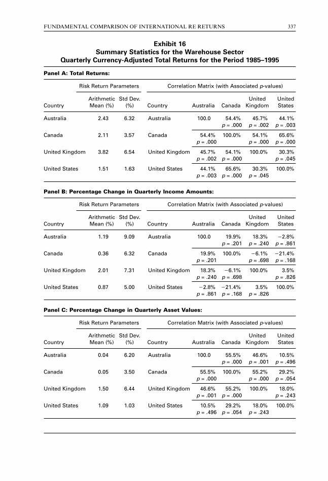
Exhibit 16

Summary Statistics for the Warehouse Sector























the capitalization rates for Canadian and U.S. warehouse property values through 1992;however there is a considerable divergence thereafter with the Canadian marketdisplaying higher values (e.g., the ending capitalization rate disparity stood at nearly 200basis points: 9.22% v. 7.29%). Meanwhile, the Australian and British warehouse sectorsdisplayed astounding volatility (with ranges of 294 and 437 basis points, respectively).Exhibit 16 provides summary statistics on the components of return as well as totalreturns.

The United Kingdom generated the highest return and volatility—and the U.S. thelowest—of the four countries examined here. This pattern was also observed in the officesector (see Exhibit 6). As with both the office and retail sectors, the concurrent cross-country returns are positively and significantly correlated (see Panel A). A ranking of thepercentage change in quarterly income amounts (see Panel B) finds the countries in thesame relative positioning as total returns, except that Canada and the U.S. have changedplaces. As before, the correlation of these changes is not as statistically significant as thecorrelation of total returns, asset values and/or capitalization rates. It is interesting thatthe percentage change in asset values (see Panel C) reveals that the Australian andCanadian warehouse sectors displayed near-zero growth, while the United Kingdom andthe United States warehouse sectors displayed growth in excess of 1% per quarter. Asnoted in Exhibit 18, the U.S. capitalization rate series for the warehouse sector hasdisplayed remarkably little variation (0.20%—see Panel D). However the U.S.capitalization rate averaged almost 200 basis points less than that realized in theAustralian market (i.e., 7.56% v. 9.45%).

The data displayed in Exhibits 13 through 16 can also be used to restate each country’stotal return from warehouse investments in terms of their underlying fundamentalcomponents of return. See Exhibit 17.

As can be seen from Panels A–D of Exhibit 17, there is remarkable consistency in therise-and-fall pattern of total returns for the warehouse sector of all four countries. Withthe exception of the U.S. warehouse sector, the initial yields cluster around 8.50%. Also,the United Kingdom clearly shows the highest growth in warehouse income. In addition,












Exhibit 17

Warehouse Index: Annualized Return Attributes from 1985:1–1995:4

1985–88 1989–92 1993–95 1985–95(4 Yrs) (4 Yrs) (3 Yrs) (11 Yrs)

(%) (%) (%) (%)

Panel A: Australia


Initial Yield 8.34 10.75 9.51 8.34

Growth in Income 9.54 27.27 3.32 2.52


Estimated Return 17.09 21.36 13.93 9.64——— ——— ——— ———

Real Estate-related Timing/Methodology Differences 0.70 3.09 22.25 0.83








Going-in Rate 8.25 8.51 10.66 8.25

Going-out Rate 8.51 10.66 10.28 10.28

Panel B: Canada


Initial Yield 8.54 7.71 8.18 8.54

Growth in Income 3.95 22.66 22.24 0.57











Going-in Rate 8.51 7.45 7.82 8.51

Going-out Rate 7.45 7.82 8.84 8.84

the United Kingdom experienced the second lowest (Canada had the lowest) adverseeffect from rising capitalization rates over the entire eleven-year period. Consequently, itshould come as no surprise that the U.K. experienced the highest returns.




1985–88 1989–92 1993–95 1985–95(4 Yrs) (4 Yrs) (3 Yrs) (11 Yrs)

(%) (%) (%) (%)



Initial Yield 8.70 7.28 10.36 8.70

Growth in Income 3.52 8.85 20.30 4.07











Going-in Rate 8.53 7.32 10.41 8.53

Going-out Rate 7.32 10.41 9.91 9.91



Initial Yield 7.47 7.24 8.46 7.47

Growth in Income 1.22 22.52 1.52 20.08






Going-in Rate 7.47 7.07 7.90 7.47

Going-out Rate 7.07 7.90 9.11 9.11

Conclusions and Recommendations

This study has analyzed the fundamental components of return (i.e., initial yield, growth inincome and shifts in capitalization rates) for the office, retail and warehouse sectors inAustralia, Canada, the United Kingdom, and the United States. These returns have beencurrency-adjusted so as to state them in terms of U.S. investors making their initial invest-ment at the beginning of 1985. It is important to examine the property sectors individuallybecause differing property mix for the total indices for these countries may obscure theextent to which the cross-country, currency-adjusted returns are similar or dissimilar.

The results of this comparison can be summarized as follows:

• Currency Returns: Though in theory currency returns should average zeropercent, dramatic swings in currency returns are observed in several subperiods.The British pound/U.S. dollar exchange rate has been particularly volatile; in theearly period, this has substantially enhanced total returns from British real estatefrom the perspective of an U.S. investor and, in the next period, has substantiallydetracted from such investments. However, on balance, currency returns havewell served the U.S. investor with holdings in the United Kingdom. Conversely,currency returns have adversely effected such holdings in Australia.

• Space Market v. Capital Market: In general, the space markets display moredivergence between countries than do the capital markets. As a measure of space-market dynamics, the path of income over the eleven-year horizon is examinedherein. As a measure of the capital markets, the path of capitalization rates isused. Compare the correlation matrices found in Panel B to those found in Cand/or D of Exhibits 6, 11 and 16. It seems appropriate to view the space markets(as proxied by earnings changes) as comprising more idiosyncratic risk as localcustoms, regulations and business practices may cause the space markets (for thesame property type) to behave differently from one country to the next.Conversely, it seems appropriate to view the capital markets as comprising lessidiosyncratic risk as the price of capital (as proxied by capitalization rates) ismore fluid and is increasingly set in international markets. As such, the path ofproperty values reflects the interaction of these two (space and capital) markets.

• Office Sector: In a pattern to be repeated for the other two property types, theU.S. office sector was the worst performing of the four countries examined here.Its poor performance can be tied directly to the persistent negative earningsgrowth and, not surprisingly, a corresponding rise in capitalization rates. In thisregard, Canada’s pattern of returns most closely resembled the U.S. However, themagnitude of these problems was less dramatic for the Canadian properties.Conversely, the Australian and British office markets actually generated positiveearnings growth. While all countries witnessed an increase in capitalization rates,the increase was most pronounced in the British and American office markets.

• Retail Sector: The Australian retail sector consistently outperformed itscounterparts in terms of total returns; this was true in all but one of the smallertime periods as well as the overall, eleven-year time period—even though U.S.investors in Australian real estate suffered adverse foreign currency fluctuations.


The differences in returns for the Australian retail sector can be traced to thehighest initial yield, the second highest earnings growth rate (only the U.K.performed better) and the most favorable shift in capitalization rates. Thereasons for the poor U.S. performance are abundant: the second lowest initialyield, the lowest earnings growth and an adverse shift in capitalization rates.Meanwhile, the British retail sector suffered the most adverse shift incapitalization rates and the lowest initial yield but enjoyed the highest earningsgrowth rate and the highest return due to currency fluctuations. Canada was“middle of the pack” in all categories.

• Warehouse Sector: The United Kingdom generated the highest return andvolatility—and the U.S. the lowest—of the four countries examined here. Thispattern was also observed in the office sector. As with both the office and retailsectors, the concurrent cross-country returns were positively and significantlycorrelated. A ranking of the percentage change in quarterly income amountsfinds the countries in the same relative positioning as total returns, except thatCanada and the U.S. have changed places. As before, the correlation of thesechanges is not as statistically significant as the correlation of total returns, assetvalues and/or capitalization rates. It is interesting that the percentage change inasset values reveals that the Australian and Canadian warehouse sectorsdisplayed near-zero growth, while the United Kingdom and the United Stateswarehouse sectors displayed growth in excess of 1% per quarter. As noted inExhibit 15, the U.S. capitalization rate series for the warehouse sector hasdisplayed remarkably little variation. However the U.S. capitalization rateaveraged almost 200 basis points less than that realized in the Australian market.

It should also be emphasized that these results are time-period specific and futurereturn patterns may materially diverge from those presented herein. Lastly, authors hopethis study stimulates future research into areas such as (1) efficient real estate portfoliodiversification in an international context, and (2) a more extensive empiricalexamination as to the degree to which the time series of international real estate returnsare co-integrated.

Appendix

As noted earlier, it is necessary to successively restate the data provider’s methodology forcomputing income and appreciation returns in terms of the imputed income and property values.The following overview of each country’s methodology (and subsequent restatement in terms ofincome and market values) uses a standardized notation, though, in practice, each country has aslightly different version.

Canada and U.S. Return Series

In order to depict this process, the Russell-NCREIF methodology for computing income andappreciation returns in Canada and the U.S. is shown below:

(1) R

NOI

MV CI PS NOIInct

t t t t− + −( )−1 5 33. ., and



(2)

where:

RInc = income return;RApp = appreciation return;NOIt = net operating income in quarter t;

CIt = capital improvements in quarter t;PSt = partial sales in quarter t; and

MVt = market value in quarter t.

In order to simplify the analytical process and to avoid the problem that the data providers do notnormally provide separate, detailed information on capital improvements and partial sales, thesecomponents are assumed to equal zero.14 Given the foregoing, the income and property valuescan be derived as follows:

(3)

(4)

Assuming any arbitrary initial investment for MV0, subsequent income and property values can becomputed by successively substituting the reported income and appreciation returns. As shownbelow, a similar “reverse engineering” process can be performed for the Australian and Britishdata series.

Australian Return Series

The BOMA of Australia methodology for computing income and appreciation returns, as shownbelow, is nearly identical to the NCREIF methodology:

(5)

(6)

As before, in order to simplify the analytical process and to avoid data disclosure problems,capital improvements and partial sales are assumed to equal zero. Given the foregoing, theincome and property values can be derived as follows:

(7)

(8) MV MV

R

Rt tApp

Inc

= ++

−1 1

1 5..

NOI

MV R

Rtt Inc

Inc

=∗

+−1

1 5., and

R

MV MV PS CI

MV CI PS NOIAppt t t t

t t t t

− + −

+ −( )−−

−

1

1 5 5. .,

R

NOI

MV CI PS NOIInct

t t t t− + −( )−1 5 5. ., and

MV MV

R

Rt tApp

Inc

= ++

−1 1

1 33..

NOI

MV R

Rtt Inc

Inc

=∗

+−1

1 33., and

R

MV MV PS CI

MV CI PS NOIAppt t t t

t t t t

− + −

+ −( )−−

−

1

1 5 33. .,


Again, by assuming any arbitrary initial investment for MV0, subsequent income and propertyvalues can be computed by successively substituting the reported income and appreciationreturns.

However, the Australian return series is only available on a semiannual basis. Therefore, inorder to assure comparability across foreign indices it was necessary to convert the semiannualreturns to quarterly returns via the following approach:

(9)

where:

∑ = semiannual return, andr = quarterly return.

It should also be noted that this multiplicative approach, while theoretically correct, produces asmall bias in the arithmetic combination of income and appreciation returns into total returns.

United Kingdom Return Series

The IPD methodology for computing income and appreciation returns, as shown below, is similarto the methodologies employed in the other countries noted above:

(10)

(11)

As before, in order to simplify the analytical process and to avoid data disclosure problems,capital improvements and partial sales are assumed to equal zero. Given the foregoing, theincome and property values can be derived as follows:

(12)

(13)

Again, by assuming any arbitrary initial investment for MV0, subsequent income and propertyvalues can be computed by successively substituting the reported income and appreciationreturns.

However, the British return series is only available on an annual basis for 1985 and 1986.Therefore, in order to assure comparability across foreign indices it was necessary to convert theannual returns (R) to quarterly returns (r) via the following approach:

(14)where:

R = annual return, andr = quarterly return.

As noted above, this multiplicative approach, while theoretically correct, produces a small bias inthe arithmetic combination of income and appreciation returns into total returns.

1 14 +( ) − =R r ,

MV MV Rt t App= +[ ]−1 1 .

NOI MV Rt t Inc= ∗−1 , and

R

MV MV CI

MV CIAppt t t

t t

− −+

−

−

1

1 5..

R

NOI

MV CIInct

t t− +1 5., and

1 1+∑( ) − = r .



Currency Returns and Currency-Adjusted Returns

The following section overviews the conversion from the domestic real estate returns into theU.S. currency-denominated returns, as identified in Exhibits 7, 12 and 17. (For a more completedescription, see Bodie, Kane and Marcus, 1992, for example.) The currency returns can becomputed quarterly in the following manner:

(15)

where:

Ôi,t = the return on the i th currency in the period t, andei,t = the spot exchange rate from the U.S. currency into the i th foreign currency at period t.

Moreover, these quarterly currency returns can be “strung together” in order to provide theannual currency return over any T periods as follows:

(16)

where:

Ei,T = the annual return on the i th currency over T periods.

The annual return of the U.S. investor who diversifies internationally (in any of the ith foreigneconomies) can be expressed as:

(17)

Accordingly, the components of the U.S. investor’s total return can also be expressed as:

Real Estate Return in Domestic Currency Ri,t

Currency Return Ei,t

Currency Returns’ Related Joint Effects Ri,t * Ei,t——————

Time-weighted Return - Currency-adjusted U.S. RU.S.,t ,————————————

as shown in Panels A–C of Exhibits 7, 12 and 17.

Notes1 The choice of the “domestic” currency is largely irrelevant. It is important, however, to recognizethat any international investor must periodically and/or eventually repatriate the foreign dollars tothe domestic currency. Otherwise, the growth of foreign net worth can be dramatically overstated:as an extreme case, consider the inflation-ridden economies of certain South American countries.2 For instance, consider the example where property mixes differ from one country to the next andthese mixes change independently over time. Such an arrangement would mask what mightotherwise represent a perfect correlation of the time series of currency-adjusted property-typereturns. 3 These semiannual returns are converted to quarterly equivalents, as described in the Appendix.4 The annual returns for 1985 and 1986 are converted to quarterly equivalents, as more fullydescribed in the Appendix.

R R EU S t i t i t. ., , , .= +[ ] +[ ]−1 1 1

Ei T

t

T

i tT

, ,/ ,+ ∏ +( ) −

=1

4 1 1ε

ε i t

i t

i t

e

e,,

,,= −−1 1


5 The NCREIF Index began as the Russell-NCREIF Index.6 However, in the absence of central bank distortions, Kritzman (1989) for example, suggests that“(a)s currencies are not productive assets, we should expect, a priori, that their returns will average0% over the long run.”7 This analysis is available from the authors.8 The authors do not necessarily suggest that this smoother path of property values (as opposed toincome values) is the result of appraisal smoothing (see Geltner, 1989, 1991; Lai and Wang, 1996).9 The p-values indicate the confidence level at which the null hypothesis can be rejected in favor ofthe alternative hypothesis: Ho: r = 0 v. Ha: r5/ 0. In the case of the office sector, the concurrentcross-country correlations are all significant at the 10% confidence level or better.10 A description of the calculation of currency returns is contained in the Appendix.11 In addition to the currency return itself, the impact of the currency returns on total currency-adjusted returns is also attributable to the cross-product of currency and real estate returns,denoted as Currency Returns’ Related Joint Effects. See the Appendix. 12 Note that the average earnings growths reported in Exhibits 9 and 10 are not directlycomparable, due to: (a) the former is restated in terms of the U.S. currency while the latter is in thedomestic currency, and (b) the former is based on the arithmetic mean while the latter is based onthe geometric mean.13 As compared to an identical investment in the respective office sectors, the Canadian and U.S.retail sectors were ravaged less (by about $45 to $50 (U.S.) per initial $100 investment).14 For the ramifications of this assumption, see Pagliari and Webb (1992).

ReferencesAsabere, P.K., R.T. Klieman and C.B. McGowan, Jr., The Risk-Return Attributes of International

Real Estate Equities, Journal of Real Estate Research, Summer 1991, 143–52.Barkham, R. and D. Geltner, Price Discovery in America and British Property Markets, Real

Estate Economics, Spring 1995, 21–44.Black, F., Exploring General Equilibrium, Cambridge, Mass.: The MIT Press, 1995.Bodie, Z., A. Kane and A.J. Marcus, Essentials of Investments, Homewood, Ill.: Irwin, 1992.Eichholtz, P.M.A., Does International Diversification Work Better for Real Estate than for Stocks

and Bonds?, Financial Analysts Journal, January–February 1996, 56–62.——— and D.J. Hartzell, Property Share, Appraisals and the Stock Market: An International

Perspective, Journal of Real Estate Finance and Economics, March 1996, 163–78.Eichholtz, P.M.A., Real Estate Securities and Common Stocks: A First International Look, Real

Estate Finance, Spring 1997, 70–74.Geltner, D., Estimating Real Estate’s Systematic Risk from Aggregate-Level Appraisal-Based

Returns, Journal of the American Real Estate and Urban Economics Association, 1989, 463–81.———, Smoothing in Appraisal-Based Returns, Journal of Real Estate Economics and Finance,

1991, 327–45.Gordon, J., Property Performance Indexes in the United Kingdom and the United States, Real

Estate Review, Summer 1991, 33–40.Hudson-Wilson, S. and J. Stimpson, Adding U.S. Real Estate to a Canadian Portfolio: Does It

Help?, Real Estate Finance, Winter 1996, 66–78.Jorion, P., Portfolio Optimization in Practice, Financial Analysts Journal, January–February 1992,

68–74.Kritzman, M., Serial Dependence in Currency Returns: Investment Implications, Journal of

Portfolio Management, Fall 1989, 96–102.Lai, T.-Y. and K. Wang, Appraisal Smoothing: The Other Side of the Story, unpublished working

paper, November 1996.



Mull, S.R. and L.A. Soenen, U.S. REITs as an Asset Class in International Investment Portfolios,Financial Analysts Journal, March–April 1997, 55–61.

Newell, G. and J. Webb, Assessing Risk for International Real Estate Investments, Journal of RealEstate Research, Spring 1996, 103–16.

———, Institutional Real Estate Performance Benchmarks, Journal of Real Estate Literature, Fall1992, 387–421.

Pagliari, J. L., Jr. and J. R. Webb, Past and Future Sources of Commercial Real Estate Returns,Journal of Real Estate Research, Fall 1992, 387–421.

———, A Fundamental Examination of Securitized and Unsecuritized Real Estate, Journal of RealEstate Research, Winter 1995, 381–426.

Quan, D.C. and S. Titman, Commercial Real Estate Prices and Stock Market Returns: AnInternational Analysis, Financial Analysts Journal, May–June 1997, 21–34.

Ziobrowski, A.J. and R.J. Curcio, Diversification Benefits of U.S. Real Estate to Foreign Investors,Journal of Real Estate Research, Summer 1991, 119–142.


a fundamental comparison of international real estate...

Documents