a free boundary problem related to singular stochastic control: the
TRANSCRIPT

COMMUN. IN PARTIAL DIFFERENTIAL EQUATIONS, 16(2&3), 373-424 (1991)
A FREE BOUNDARY PROBLEM RELATED TO SINGULAR STOCHASTIC CONTROL:
THE PARABOLIC CASE
H.M. Sonerl
S.E. Shrevez
Department of Mathematics Carnegie Mellon University
Pittsburgh, PA 15213
1. INTRODUCTION
This paper concerns the existence of classical solutions to the
nonlinear partial differential equations.
a a (1.1) max { p ( x , t ) - ~ u ( x , t ) - h(x,t), u(x,t) - f(t)} = 0, x d ' , t > 0,
n
with a forcing term h which is convex i n the xn-variable. Under
appropriate smoothness and growth conditions on the data, we prove the
existence and the uniqueness of polynomially growing, positive, classical
solutions to (1.1) for every initial condition
which is also convex i n the xn-variable. Moreover, we obtain the Lipschitz
373
Copyright @ 1991 by Marcel Dekker, Inc
Dow
nloa
ded
by [
ET
H Z
uric
h] a
t 02:
40 1
1 Ju
ne 2
012

SONER AND SHREVE
continuity of the free boundary of the region in which the parabolic equation
u - A U - h = 0 holds. t
The w ~ ' ~ regularity in the spatial variables and the boundedness of l o c
the time derivative was proved by Chow, Menaldi, Robin [6], Menaldi, Robin
[22] and Menaldi, Taksar [23]. They used control-theoretic techniques along
with the convexity assumption. Also, the stationary version of (1.1) was
recently studied by the authors [27], and part of the present analysis closely
follows 1271. As in [27] our approach to (1.1) is to first solve the obstacle
problem
with initial condition
The convexity assumption on the data enables us to show that
and we construct u by integrating the above relation. Known regularity
results for (1.3), ([3],[9],[11]), with several estimates of the free boundary,
2 1 n yield u E C ' ([R x(0,rn)) (twice continuously differentiable in the spatial
variables and once continuously differentiable in the time variable). In the
context of one-dimensional stochastic control the connection (1.5) goes back
to Bather and Chernoii [2] and has been given probabilistic explanations by
Dow
nloa
ded
by [
ET
H Z
uric
h] a
t 02:
40 1
1 Ju
ne 2
012

A FREE BOUNDARY PROBLEM 375
Karatzas and Shreve [19], El-Karoui and Karatzas [7], and analytical
derivations by Karatzas [16], Chow, Menaldi and Robin [6], Menaldi and
Robin [22]. Without the convexity assumptions, (1.5) is no longer true, and
in general (1.1) does not have classical solutions.
The related elliptic problem
(1.6) max {u(x) - AU(X) - h(x), I Vu(x) I - 1) = 0,
was studied on a bounded domain by Evans [8] and then by Ishii and Koike
[Is]. Evans obtained solutions in w21m via penalization and the maximum l o c
principle. In fact this regularity result is sharp in the absence of convexity.
However, for (1.6) in two dimensions with a convex forcing term h, the
authors recently obtained a classical solution [28]. Due to the nonlinearity
of the constraint in (1.6), the obstacle problem related to it is more
complicated than (1.3) and techniques in [28] are different from the ones
employed here and in [27].
Equation (1.1) is the dynamic programming equation related to a
singular stochastic control problem. Briefly, the problem is to optimally
control an n-dimensional Brownian motion by pushing only along the
(0,0,..,-1) direction. In this context, the solution to (1.1) and (1.2) is the
value function for the finite horizon control problem in which h is the
running cost, g is the terminal cost and, at time t , f(t) times the
displacement caused by the push is equal to its cost. This problem is
formulated and solved in Section 7. The reader may refer to Shreve [25] for
an introduction to this kind of control problems.
In singular stochastic control literature, the spatial c2 regularity of
the value function has been called the "principle of smooth fit" by Benei,
Dow
nloa
ded
by [
ET
H Z
uric
h] a
t 02:
40 1
1 Ju
ne 2
012

3 76 SONER AND SHREVE
Shepp and Witsenhausen [ I ] . It has been instrumental in the analysis of
several one-dimensional problems [ 7 ] , [12] , [13] , [14] , [17] , [18] , [19] , [26].
The paper is organized as follows: results related to (1 .3 ) are stated
in the next section and the Lipschitz continuity and the boundedness of the
free boundary are obtained in Sections 3 and 4. Section 5 is devoted to the
constr,uction of a classical solution to (1.1) and its uniqueness is proved in
Section 6. The related singular stochastic control problem is defined and
solved in Section 7 . Finally, we analyze a penalization of (1 .3 ) in the
Appendix.
2. AN OBSTACLE PROBLEM
In this section we study the solutions to equation (1 .3 ) with initial
data (1 .4) . Subscripts i and t denote the differentiation with respect to xi
and t , respectively. We assume
(2 .1) h,g, and f are three t imes differentiable, non-negative with
f(t) 2 1 for all t 2 0. Moreover, these junctions, together with
their derivatives up to order three, grow at most polynomially as
I X I and t tend to infinity;
and
there is a n a > 0 such that
Dow
nloa
ded
by [
ET
H Z
uric
h] a
t 02:
40 1
1 Ju
ne 2
012

SINGULAR STOCHASTIC CONTROL
for every x€Rn, t > 0; and
for every XER"
Theorem 2.1 There is a zcnique solution v to (1.3) and (2.4) satisfying
with suitable positive constants K,m. Henceforth we shall use v to denote
the solution of (1.3) and (1.4) satisbing (2.4).
The above regularity result of solutions to (1.3) and (1.4) is now
standard in the nonlinear partial differential equations literature. A similar
result for the one phase Stefan problem was obtained by Friedman and
Kinderlehrer [ll], and a modification of their proof yields the above result.
Also see [3], 141, [5], [lo], [29], [30]. For the sake of completeness, we give the
proof in the appendix. To establish notation, we begin the proof here.
Consider the following penalized version of (1.3)
The penalization term PC is given by PC(,) = p(r/ t) for some smooth
Dow
nloa
ded
by [
ET
H Z
uric
h] a
t 02:
40 1
1 Ju
ne 2
012

3 78
function p satisfying
SONER AND SHREVE
Let v t be the solution to (2.5)' with initial data (1.4). The following
theorem is proved in the Appendix.
Theorem 2.2. There are positive constants K,m, independent of c, such
that vE satisfies (2.4) with these constants. Moreover v' converges to v
uniformly on bounded sets.
3. LIPSCHITZ CONTINUITY OF THE FREE BOUNDARY.
In this section we study the spatial boundary of the region
We discover, in Section 4, that for fixed (xl,.. , x ~ - ~ ) and t > 0, the region
d is bounded above in the xn-coordinate. However, this upper bound may
approach infinity as t tends to zero. We show here that the boundary of $
admits a lipschitz continuous parametrization. Our method is to obtain a
uniform Lipschitz estimate for parametrizations of the boundaries of an
approximating sequence of regions
Dow
nloa
ded
by [
ET
H Z
uric
h] a
t 02:
40 1
1 Ju
ne 2
012

A FREE BOUNDARY PROBLEM 379
Lemma 3.1. For E > 0, fhere is a continuously dzffe~entiable jhction
q' :In-' x (0,m) -, I such that
Proof. Differentiate (2.5)' with respect to x n to obtain
Since @; is bounded, @; and the initial condition V:(X,O) = gnn(x) are
non-negative and hnn 2 a > 0 , the maximum principle yields that for each
t > 0 , vi(x,t) is bounded below by a positive constant, uniformly in x.
Thus qc(y,t) k inf {xnl ~ ' ( ~ , x ~ , t ) 2 f(t)) is finite. Since the boundary of
dc in Px(0,m) is the zero level curve of the function v6(x,t) - f(t), the
differentiability of q' is a direct consequence of the implicit function
theorem and the strict positivity of v i . o
We proceed to obtain a uniform Lipschitz estimate of q'. We need
several estimates of the derivatives of v'.
Lemma 3.2. There is a posative constant K, independent of E, such that
for every x€In, t > 0, i= l , ..., n-1.
Proof. Differentiate (2.5)' with respect to xi:
Dow
nloa
ded
by [
ET
H Z
uric
h] a
t 02:
40 1
1 Ju
ne 2
012

3 80 SONER AND SHREVE
€ (3.6) ~:~(x,t)+Q(v"x,t) - f(t))v:(x,t) - dvi(x,t) = hni(x,t).
1 1 Assumption (2.2) yields that I v;(x,0) I = I gni(x) I < , gnn(x) = , vn(x,O) . 1 Also, 1 hni(x,t) I < a hnn(x,t). Hence the maximum principle, together with
(3.4) and (3.6), implies (3.5) with K = l / a .
Lanma 3.3. There are positive constants K,m, independent of c, such that
t (3.7) Ivi(x,t) - f'(t)I 3 K ( l + l x ~ ~ ~ ) v:(x,t)
for every x E [in, t > 0.
Proof. Theorem 2.2 and assumption (2.1) yield the existence of a positive
constant C and an integer m > 1 such that
(3.8) ~v i (x , t ) - ~ ( t ) 1 5 et(c+ f 1 x 1 ~ ~ ) .
For xo E Rn we define an auxiliary function 4 by
t #(x,t) = t (vf(x,t) -fl( t)) - e ~ x - x ~ l ~ ~ .
It should be noted that 4 actually depends on xo but this dependence is
suppressed in the notation. We calculate directly that
I(x,t) Qt(x,t) + Pi(. . .) 4(x,t) - ~ 4 ( x , t ) =
= t [vit(x,t) - ~ v i ( x , t ) + 4 ( . .)(v;(x,~) - ft( t))] - t f
Dow
nloa
ded
by [
ET
H Z
uric
h] a
t 02:
40 1
1 Ju
ne 2
012

A FREE BOUNDARY PROBLEM 381
t + e [-I x-xo 1 2m + 2m(2m+n-2) 1 x-xo I 2(m-1) - p f ( . 6 a ) 1 x-xo 1 2 m ~
where (. - .) denotes vC(x,t) - f(t). Use (3.8), equation (2.5)' and the
positivity of p;(- - a ) to obtain
We estimate the above terms by using the assumption (2.2) and the
! inequalities t i
Dow
nloa
ded
by [
ET
H Z
uric
h] a
t 02:
40 1
1 Ju
ne 2
012

382 SONER AND SHREVE
The latter inequality is obtained by observing that its left-hand side is I -1
maximized over x by x = (1 - 2- zm-1) xo. Hence, we have
where Cm = C + 22m-1 (m-l)(m-l) ( ~ m + n - 2 ) ~ and
1 A -(2m-1) Bm = $2 m- - 1)
Since hnn(x,t) 2 a, the above inequality yields
Recall that I(x,t) = qj(x,t) + @;( . . ) $(x,t) - ~ # ( x , t ) . Hence (3.4) shows 1 that fi(x,t) b $(x,t) - [T + (C,+Bm I x0 1 2m)eT]vi(xlt) satisfies
The maximum principle now implies
Dow
nloa
ded
by [
ET
H Z
uric
h] a
t 02:
40 1
1 Ju
ne 2
012

A FREE BOUNDARY PROBLEM
Therefore
-T Set K = max {B,, max{Te + Cm : T > O}}/a.. Then the above
inequality implies that
To prove the reterse inequality we consider the auxiliary function
and proceed exactly as before. o
Lemma 3.4. There are positive constants K,m, independent of 6, such that
i n f q'(y,t) > - m € > O
for all y ~ ~ ~ n - l , t > 0.
Proof. Use two characterizations, (3.2) and (3.3) of d E to obtain the two
Dow
nloa
ded
by [
ET
H Z
uric
h] a
t 02:
40 1
1 Ju
ne 2
012

384 SONER AND SHREVE
different expressions for the unit normal vector z6(x,t) at a boundary point
(x,t) E a a€,
t z (x,t) = (vv' (x, t 1, vf(x,t) - f ' ( t))
where for any x = (xl, ... , x,),
The above identity yields that for any (x,t) E 8 dt,
and vf (x,t) - f ' ( t) = - qt( i , t ) vA(x,t). Combine these identities with (3.5) t and (3.7) to arrive at (3.11) and (3.12).
We continue by obtaining a lower bound for qE(y,t). First consider
the equation
(3.15) Vt(x,t) - ~ V ( x , t ) = hn(x,t)
Dow
nloa
ded
by [
ET
H Z
uric
h] a
t 02:
40 1
1 Ju
ne 2
012

A FREE BOUNDARY PROBLEM 385
with i f i t i d data V(x,O) = gn(x). Since vc(x,t) is a subsolution to the above
equation, the maximum principle yields that
Differentiate (3.15) with respect to xn to obtain Vnt(x,t) - AV,(X,~) =
hnn(x,t) 2 a and Vn(x,O) = gnn(x) > 0. Hence,
for all x a n , t 2 0, and consequently Q(y,t) inf {xn : V(y,xn,t) > f(t)) is
finite for every ydRn-l, t > 0. However (3.16) yields qc(y,t) 2 Q ( Y , ~ ) . o
For a positive integer m, we define qc,m by qclm(y,t) = c,m . min {qc(y,t), m}. The previous lemma shows that for each m, q IS
locally Lipschitz continuous, uniformly in c. By using a diagonal argument
we may choose a subsequence, denoted by c again, along which qc'm
converges to a Lipschitz continuous function qm for each m. Finally let
q(y,t) be the increasing limit of qm(y,t). This limit may take the value
+m, but this possibility is ruled out in the next section. Indeed, the local
boundedness of q proved in Theorem 4.2, together with the local Lipschitz
continuity of qm, implies local Lipschitz continuity of q on mn-' x (0,m).
The following "sharper" lower bound for q(y,t) shall be used in
Section 5.
Lemma 3.5. For each T > 0, there is a positive constant K ( T ) such that
Dow
nloa
ded
by [
ET
H Z
uric
h] a
t 02:
40 1
1 Ju
ne 2
012

386 SONER AND SHREVE
where K 0 is as in (3.11).
Proof. In view of (3.11) and (3.17), it suffices to show that
inf Q(0,t) > a, O<t<T
for every T > 0. Observe that Q(y,t) is the zero level curve of V - f and
Vn > 0 on IRn x ( 0 , ~ ) . Hence by the implicit function theorem, Q is
continuous on IRnx(0,w). Moreover, due to the assumption (2.3) and the fact
that V(x,O) = gn(x),
Hence, lim inf Q(y,t) > -m. t +O
Corollary 3.6. We have
In particular, q is independent of the subsequence along which the limit is
taken.
Proof. It suffices to show that bm = d m, where
Dow
nloa
ded
by [
ET
H Z
uric
h] a
t 02:
40 1
1 Ju
ne 2
012

A FREE BOUNDARY PROBLEM 387
for every m. Let ( j , i n , f ) E d be given. Since q'im converges to q m
uniformly on bounded subsets, there are to > 0 and a neighborhood J' of
(?,in,€) such that
Therefore vC(x,t) < f(t) and v;(x,t) - nvf(x,t) = hn(x,t) for all (x,t) E X
and 0 < E < rO. By letting 6 go to zero we obtain that v(x,t) < f(t) and
vt(x,t) - ~ v ( x , t ) = hn(x,t) for all (x,t) E J'. Differentiating the last
equation with respect to xn and then using the positivity of hnn and the
non-negativity of vn , we obtain that vn > 0 on 1. Hence v < f on X
and consequently ( j,Pn, t ) E dm.
To prove the reverse inclusion, let (?,in,€) be an element of gm.
Then v ( j , G , t ) < f(f) and the convergence of v' to v implies that
fn < q''m(f,t) for all sufficiently small 6. Letting E go to zero, we
conclude that (F,i,,f) s closure (d m). Since im is an open set,
dm C interior (closure ( d m)). But the right-hand side is equal to d m,
due to the Lipschitz continuity of qm. o
Remarks
1. In one space dimension, Van Moerbeke obtained the smoothness of the
free boundary under quite different structural assumptions 1291, [30]. Van
Dow
nloa
ded
by [
ET
H Z
uric
h] a
t 02:
40 1
1 Ju
ne 2
012

3 88 SONER A N D SHREVE
Moerbeke uses an integral equation satisfied by the parametrization of the
free boundary to obtain local existence, and then he obtains the global result
by deep stochastic analysis. In the multi-dimensional case it is also possible
to obtain an integral equation for the parametrization. However it seems to
be of little use because of its very complicated structure.
2. In the stationary case [27], the authors proved the smoothness of the free
boundary by applying theorems of Caffarrelli [5] and Kinderlehrer and
Nirenberg [20], after its Lipschitz continuity was established. However, the
results of Section 2 of [5] are not directly applicable to the problem under
investigation.
4. AN UPPER BOUND FOR q
We start by analyzing the zero-level curve of v(x,t) + 1. Let
(4.1) G(y,t) = inf {xn: v(y,xn,t) 2 -1)
Because l im V(y,xn,t) = - m (see (3.17)), and X -t - m n
v(x,t) = l i m vc(x,t) 5 V(x,t) €1 0
(see (3.16)), we know that G(y,t) > - m.
Lemma 4.1. For T > 0 there is a constant C(T) such that
(4.2) i ( ~ > t ) l C(T) ( l Y l + 1)
for all y ~ ~ n - l and t6 [0, T j .
Dow
nloa
ded
by [
ET
H Z
uric
h] a
t 02:
40 1
1 Ju
ne 2
012

A FREE BOUNDARY PROBLEM 389
Proof. Consider the linear equation with initial condition
where -(a)- 4 min {a,O). Since f(t) 2 1 and Y(x,t) 5 0, Y is a
subsolution to (2.5)' for each 6 > 0. Hence Lemma 8.1 of the appendix
yields that Y(x,t) 5 vC(x,t) for every c > 0 and therefore
Moreover,
Also the assumption (2.2) yields that
for every ydRn-l and t > 0. A simple application of the monotone
convergence theorem yields that 1 i m Y(y,x,,t) = 0 for every y dRn-' X + m n
and t 2 0. This together with (4.4) implies that q(y,t) < m. We claim that
there is C(T), such that
Dow
nloa
ded
by [
ET
H Z
uric
h] a
t 02:
40 1
1 Ju
ne 2
012

390 SONER AND SHREVE
Indeed, vn(y,h(y,t), t ) > 0 for ysRn-l and t > 0, becausein a
neighborhood of (y,i(y,t),t) we have vnt - AV = h n nn > 0. By the
implicit function theorem, ij is smooth, in particular continuous, on
Rn-' x (0,m). We also have the inequality at the initial point
lim sup ij(0,t) < sup {xndR: gn(O,xn) 5 -1) < m. t 10
The above inequality together with the continuity of 6 on the open domain p-1 ~(0,m) is enough to arrive at (4.5).
Proceeding exactly as in the proof of Lemma 3.4, we can show that
Now let C(T) = max {c(T), C).
Theorem 4.2. The function q(y,t) is locally bounded in (IJ,~) E Rn-I x (0,m).
Proof. Fix T > 0 and then chose a positive constant C 2 1 satisfying
Define
A k(y,t) = inf {xn : hn(y,xn,t) - f'(t) 1 0)
Dow
nloa
ded
by [
ET
H Z
uric
h] a
t 02:
40 1
1 Ju
ne 2
012

A FREE BOUNDARY PROBLEM
and note that because hnn > a > 0, k(0,t) is bou nded uniformly in
t E [O,T] and k is differentiable. From (2.2) and the argument used to
prove (3.11), we can show that for some constant C, which also satisfies
(4.6), (4.7), we have
k(y,t) < C(( y 1 + l ) V(y, t )~ [O,T].
It follows that
(4.8) hn(y,xn,t) - f '(t) 2 ff [xn - C( l Y l +l)l + hn(y, C( l Y l +I ) , t ) - f ' ( t )
> ff x - ( 1 y 1 v y d - ' , xn > C(l y 1 + l ) , t E [O,T]. -
It is elementary to construct a smooth function r] satisfying
We continue by constructing a subsolution to (1.3). First consider the
following equation with arbitrary constants K > /I' 2 0, and C as in
(4.6)-(4.10):
y i th boundary condition #(O) = 0. An explicit formula for the solution #
is
Dow
nloa
ded
by [
ET
H Z
uric
h] a
t 02:
40 1
1 Ju
ne 2
012

392 SONER AND SHREVE
where ro is the solution to the transcendental equation
The following properties of 4 rather than the explicit formula for it
will be used in the analysis:
(4.13) (i) q5,q5/ are Lipschitz continuous,
Set
(4.14) (i) a * = A 1 - f(0) + max f(t), O < t < T
(4.14) (ii) K 4 2(f(0)+2) e-T T-l,
(4.14) (iii) P K/2,
where jT = (xl,.. , x,..~) when x = (xl, ... , xn). Finally define
Dow
nloa
ded
by [
ET
H Z
uric
h] a
t 02:
40 1
1 Ju
ne 2
012

A FREE BOUNDARY PROBLEM
n 4 {(x,t) : o < t s T , R(X) > o
and define w on TI by
where 4 is as in (4.12) with K and /3 given in (4.14).
We claim that w is a subsolution of (1.3) on the region n . Indeed,
using (4.15) and (4.11), we calculate that
Using (4.13) (ii) with (4.10), then (4.11) and (4.14), we arrive at,
Also, for (x,t) E n , (4.8) and (4.9) imply that
Substitute the above inequality into (4.16) to obtain Dow
nloa
ded
by [
ET
H Z
uric
h] a
t 02:
40 1
1 Ju
ne 2
012

394 SONER AND SHREVE
This shows that w is a subsolution of (1.3) on n. We now show that w 5 v on the parabolic boundary of n. Due to
(4.71,
From the definition of R, we see that R(x) = R(f,O) + xn for all x@. In
particular, (y,-R(y,O)) E Kl for each y ~ ~ n - l . Now (4.1), (4.6), (4.9) and
the negativity of vn imply that
In the last inequality we have used the fact that
Taken together, (4.19) and (4.20) imply that w < v on the parabolic
Dow
nloa
ded
by [
ET
H Z
uric
h] a
t 02:
40 1
1 Ju
ne 2
012

A FREE BOUNDARY PROBLEM
boundary of fl. Hence the m
w(x,t) < v(x,t), V(x,t) E R.
Recall that q5(rO) = P.
(y,r0 - R(Y,O),T) gives
395
mimum principle, Lemma 8.5, yields that
Hence the above inequality used at the point
Hence v(y,ro - R(y,O),T) = f(T), and consequently q(y,T) < ro - R(y ,O)
Remark. A similar result was obtained by Karatzas [17], Section 7, in the 2
one-dimensional special case of h(x,t) = x .
5. c2J REGULARITY OF n
Let U(x,t), V(x,t) be the polynomially growing solutions of
with initial conditions
(5.3) U(x,O) = g(x), xmn.
(5.4) V(X,O) = g,(x), x a n .
Dow
nloa
ded
by [
ET
H Z
uric
h] a
t 02:
40 1
1 Ju
ne 2
012

SONER AND SHREVE
For x a n and t 0, define u(x,t) by
where as in the previous sections Z = ( x l , .., x ) and v is the solution of n-1 (1.3) and (1.4). The integrability of v-V , required by (5.5), is a part of the
following theorem.
Theorem 5.1. The finction u(x,t) is welddefined, twice continuously
differentiable in the spatial variables and once continuously differentiable in
the t-variable. Moreover, it is a solution to (1.1) and (1.2).
We need the following lemma in the proof of the above theorem. For *
positive constants K ,T, set
Lemma 5.2. Suppose that a continuous function cp, defined on all of * *
[Rnx[O,~), satisfies the following with suitable positive constants K ,C , T
and m _> 1:
Dow
nloa
ded
by [
ET
H Z
uric
h] a
t 02:
40 1
1 Ju
ne 2
012

A FREE BOUNDARY PROBLEM
(5.6) (iii) p(x,0) = 0, VXELR",
(5.6) (iv) I P ( X , ~ ) I r C * ( I X I ~ ~ +I), v(x,t) E w*,T).
Then, for every y ~ ~ n - l , te[O,T], the findion xn H p(y,xn,t) is absolutely
integrable on any interval of the form (- m, a].
Proof. Set
X [ e x ~ ( x ~ + ~ ~ E Jc{l,. . ,n-I} ~ E J
We directly calculate that
Dow
nloa
ded
by [
ET
H Z
uric
h] a
t 02:
40 1
1 Ju
ne 2
012

3 98 SONER AND SHREVE
* * where (...) = xn + K C yi - K 2: yi. Since both 1 y 1 2(m-1) and
i€J i t J
I Y I 2m-1 are bounded from above by 1 y 1 2m + 1, the definition of A yields
that the above expression is non-negative. Hence
Moreover, using the definition of II, and (5.6) (iv) we obtain
2 C* [ ( l + ( ~ * ) ~ ( n - l ) ) ~ ( l y 1 2m + l ) ]
for all y ~ ~ n - l , t E[O,T]. Also, +(x,O) ) 0 = ( dx,O) 1 . Since $ is growing *
at most polynomially on n(K ,T) and it dominates 191 on the parabolic *
boundary of 62(K ,T), the maximum principle yields that
Proof of Theorem 5.1.
Fix T > 0 and let K(T) be the constant appearing in (3.18)
Dow
nloa
ded
by [
ET
H Z
uric
h] a
t 02:
40 1
1 Ju
ne 2
012

A FREE BOUNDARY PROBLEM
Define
dy ,xn , t ) = v(y,xn - WT), t ) - V(y,xn-K(T), t).
Due to the estimate (3.18), equations (1.3) and (5.2), boundary conditions
(1.4) and (5.4), and the polynomial growth estimate (2.4), p satisfies the
hypothesis of the previous lemma. Hence u(x,t) is well-defined. Similarly
p , p, p . satisfy the hypothesis of Lemma 5.2 for each i , j = 1, . , n. Hence t 1 1J
In view of (5.1), (5.2), we have
Now using (1.3) and the fact that un = v, we conclude that u is a solution
of (1.1). Also u satisfies (1.2).
To complete the proof of the theorem, it suffices to show that the
integral terms in (5.8) and (5.9) are continuous in (x,t). For b > 0,
approximate the integral in (5.8) by
Dow
nloa
ded
by [
ET
H Z
uric
h] a
t 02:
40 1
1 Ju
ne 2
012

SONER AND SHREVE
On xn > q(?,t] , vt = f ' , and hence the second integral is continuous.
The continuity of the first integral follows from the parabolic regularity.
6 Hence F is continuous for each positive 6 and
6 Therefore, F + Ut converges to ut uniformly on bounded subsets, and ut
is a continuous function. The continuity of u.. is proved similarly. o 'J
6. UNIQUENESS
We start with a comparison result. This proof is related to the
uniqueness proof of Evans [B].
2,l n Ikmma 6.1. Suppose that U, u E C ([A x(0,m)) fl c ([Anx[O,m)) are sub and
supersolutions to ( 1 . 1 ) and (1.2). Further assume that for any T > 0 there *
are positive constants C ,m such that for all t €[O,T],
Dow
nloa
ded
by [
ET
H Z
uric
h] a
t 02:
40 1
1 Ju
ne 2
012

A FREE BOUNDARY PROBLEM
and
- * (6.2) un(x,t) < f(t) whenever xn < - C (1 + 1x1 )
Then
(6.3) u(x,t) < K(x,t) .
Proof. Fix T > 0. Consider the auxiliary function
where 6 > 0 is a small parameter,
1 2 <(I) A e l r / - / r l - T I , Vr€(-m, a),
and 7 is a smooth function satisfying
with the constant C-' appearing in the hypothesis of the lemma. Since ( is 6 exponentially growing, q5 achieves its maximum over R n x [ O , ~ ] , say at
* * * 6 * * (x ,t ). If t = 0, then I$ (x ,t ) < 0. Otherwise,
Dow
nloa
ded
by [
ET
H Z
uric
h] a
t 02:
40 1
1 Ju
ne 2
012

402 SONER AND SHREVE
* * * Since gn 5 f and ('(r) 2 0 for r 2 0, we have s ( x ,t ) < f(t ) if * * * * * *
x q * ) . But if xn < -q(x ), Gn(x ,t ) < f(t ) due to (6.2) and * *
(6.5)(i). Hence at (x ,t ), iin < f and
Then using (6.6) and the fact that u is a subsolution we obtain that
where
6 A K (x) = 6 B (" ( h i ) + 6 (1+ 1 vq(2) / 2, 1'' (6 [xn+q(i)])
i = l
Using the inequalities (6.5)(ii), [ (' I <_ 5c and (" <_ 5<, we estimate
~ ~ ( 4 by
for some suitable constant C > 0. Substitute the above estima,ts into (6.7)
Dow
nloa
ded
by [
ET
H Z
uric
h] a
t 02:
40 1
1 Ju
ne 2
012

A FREE BOUNDARY PROBLEM
to obtain
Send 6 to zero to arrive at (6.3). o
Corollary 6.2. The function u defined by (5.5) is non-negative and
polynomially growing.
Proof. The fact that u is polynomially growing follows from the
polynomial growth of U,V and v. Let u : 0, and ii = u in the previous
lemma. Since g,h 2 0, - u is a subsolution. Also, Lemma 3.5 implies that - - u = u satisfies (6.2). Hence, u = u 2 u = 0. o
Theorem 6.3. There is a unique polynomiaUy growing, non-negative,
(classical) solution of (1.1) and (1.2), and it is defined by (5.5).
Proof. In view of the previous results it suffices t o show that any
polynomially growing, non-negative solution of (1.1) and (1.2) satisfies (6.2).
Indeed let u(x,t) be such a solution and for ytP-l, t 0, define xn(y,t)
and P ( Y , ~ ) by
A where G(x,t) = ut(x,t) - bu(x,t) - h(x,t). We claim that xn(y,t) ? p(y,t)
for all y ~ l ~ n - l and t 2 0. Indeed, if this inequality does not hold for s.ome
Dow
nloa
ded
by [
ET
H Z
uric
h] a
t 02:
40 1
1 Ju
ne 2
012

4 04 SONER AND SHREVE
* * * * * * y ,t , then there is 6 > 0 such that G(y , p(y ,t ) - 6, t ) < 0. By the
* * * * continuity of G, there is a neighborhood of (y , p(y ,t ) - 6, t ) on which
G is strictly negative. Hence on this neighborhood un = f, A U ~ = 0 and
The above inequality and the argument leading to it imply that * * * * * * *
G(y ,xn,t ) < 0 and un(y ,xn,t ) = f(t ) whenever xn 5 p(y ,t ) - 6. But
this contradicts the positivity of u. Hence xn(y,t) 2 p(y,t). The
assumption (2.2) yields that p(y,t) 2 --C(T)(l y 1 +I), vy€lRn-l, t€[O,T] for a
suitable constant C(T). This shows the existence of a constant C(T) such
that ut(x,t) - ~ u ( x , t ) - h(x,t) = 0 whenever xn 5 - C(T) (1+ 1x1). But on
the set where this equality holds, unn > 0 and un f, so in fact un < f
whenever xn < - C(T)(l+ 1x1). u
7. THE SINGULAR STOCHASTIC CONTROL PROBLEM. 1 Consider the stochastic process Xs = (X8, ..., x:) EP defined by
Xs = x +p Ws - ((s) en, s 2 0,
where x d is the initial condition, Ws = (w:,. ..,w:) E lRn is an
n-dimensional standard Brownian motion , en = (0,0, ..., l)€lRn, [(s) is the
control process, which is non-decreasing, left-continuous, adapted to the
augmentation by null sets of the filtration generated by W, with ((0) = 0.
Dow
nloa
ded
by [
ET
H Z
uric
h] a
t 02:
40 1
1 Ju
ne 2
012

A FREE BOUNDARY PROBLEM 405
For a given initial condition x a n and horizon t > 0, the control
problem is to select a control process so as to minimize the cost functional
* Finally define the value function u by
* u (x,t) i n f J(x,t,t(.)).
C(*)
* THEOREM 7.1. The value finction u (x,t) is the unique, non-negative,
polynomially growing solution of ( l . l ) , (1.2). Moreover, the infimum in (7.1) *
is achieved by the left-continuous process 5 given by
where q is as in Corollary 9.6.
Proof. Let u be the solution to (1.1), (1.2), and let U be as defined in
Section 5. We develop some preparatory results. Define F(x,t) 4 U(x,t) - *
u (x,t), and note that for 6 2 0, Dow
nloa
ded
by [
ET
H Z
uric
h] a
t 02:
40 1
1 Ju
ne 2
012

SONER AND SHREVE
> inf [(U(x,t) - J(x,t,((.))) - ( ~ ( x - k n , t ) - ~(x-kn,t,((.)))] - (( -1
C
= inf E{I [ h ( x + P Ws,t-s) - h ( x + P Ws - ((s) e"Pt-1 ( ) 0
- h ( x + P W, - 6 en,t-s) + h(x+ p Ws - ((s) en - 6 en,t--s)]ds
due to the convexity of h and g. Thus, F(x,t) is nondecreasing in the xn -
variable. Note also, from It& lemma, that with ( an arbitrary control
process and rm inf {a 2 0: I Xs I > m} we have
+ E I: (u(X,,t-e)- u(xs+,t+)- un(xs,t-s)[t(s+)- ((~11) O<s<thrm
+ E u(XtAT,, t - tArm).
Using (1.1), (1.2) and the convexity of u in the xn- variable, we obtain
from (7.3)
Dow
nloa
ded
by [
ET
H Z
uric
h] a
t 02:
40 1
1 Ju
ne 2
012

A FREE BOUNDARY PROBLEM
tArm (7.4) u(x,t) 5 E{S [h(Xs,t+)ds + f(t-s)d((s)] + g(Xt)}
0
+ E {(u(Xr , t - ~ ~ ) - g (XtN xir < t}l> m m
where xA denotes the indicator of the set A. If we take ( 2 0, then
Xt = x + p Wt and (7.4) implies
t Arm (7.5) u(x,t) 5 1 i m ~ { j h(x + CZ Ws, t s )ds + g(x +P Wt)}
mTm 0
t = E {I h(x + p Ws,t-s)ds + g(x + p Wt)} = U(x,t).
0
Now let an arbitrary control process ( be given. We shall show that
and so we assume without loss of generality that J(x,t,((.)) < m. This ,
implies that
from which we have
Dow
nloa
ded
by [
ET
H Z
uric
h] a
t 02:
40 1
1 Ju
ne 2
012

t r 1 i m E l (h(Xs,t-s)ds + f(t-s)dt(s)) = 0.
m-.m thrm
From (7.4), (7.5) and the definition of J(x,t,((.)), we have
and (7.6) will follow from (7.7) provided we show
(7.10) lim SUP E [F(Xr ,t-rm) X i T < tl] 5 0. m+m m m
Recalling that F(x,t) is nondecreasing in the xn- variable, we may write
lim sup EIF(X ,t-'m)x{rm< ql m-tn 'rn
m* m
Dow
nloa
ded
by [
ET
H Z
uric
h] a
t 02:
40 1
1 Ju
ne 2
012

A FREE BOUNDARY PROBLEM
< lim sup E[U(x + W ,t-rm) q, < tl] = 0 - m-m 'm m
because U grows polynomially and 7, f t . This completes the proof of
(7.6) for arbitrary (, from which we immediately conclude that u(x,t) I *
u (x,t). *
To prove the reverse inequality, let ((.) be the control process *
defined in the statement of the theorem and let X. be the state process *
corresponding to it. The following follows from the definition of E :
* (7.11) (i) (Xs, t s ) E 9 for all s E (O,t],
* * (7.11) (ii) X . , ( (.) are continuous on (O,t],
* Using (7.11) in (7.2) we arrive at u(x,t) = J(x,t,( (.)). 0
8. APPENDIX
For c > 0, there is a smooth, polynomially growing, positive solution
v' to (2.5)' and (1.4). Such a solution is constructed as the limit of
solutions to a sequence of boundary-value problems. See Sections 5.6 and
5.8 in Ladyzenskaya et al. [21], especially Remark 8.2 on page 496. Also, the
details of such an approximation for an elliptic problem are given in the
Appendix of [28].
Dow
nloa
ded
by [
ET
H Z
uric
h] a
t 02:
40 1
1 Ju
ne 2
012

SONER AND SHREVE
The results of this section are either known or are obtained by slight
modification of the proofs of known results. The reader may refer to [3], [4],
151, [6], [a], [9], [lo], [ l l ] , [22], [23]. However, none of these references
provides the results we need under precisely the conditions of our model.
Our analysis is closely related to the one in Evans [a], especially the proofs of
Lemma 8.3 and 8.4 below. We start with a comparison result for equation
(2.5)'.
lemma 8.1 Suppose that 1, 7 c c2j1 (LRnx(O,m)) f l c ( o I ~ ~ [ o , ~ ) ) are
polynomially growing sub and supersolutions to (2.5)' , respectively. Then, for
all (x,t) an x [Op),
- (8.1) v(x,t) - v(x,t) j et sup (V(Z,O) - V(Z,O))+
ZER"
Proof. Since 1 and ii are polynomially growing, for each 6 > 0 there is
m 2 1 such that the function
* * * achieves its maximum on IRnx[O,m) at some point (x ,t ). If t = 0, then
* (8.1) holds, so we may assume that t > 0. Then
Dow
nloa
ded
by [
ET
H Z
uric
h] a
t 02:
40 1
1 Ju
ne 2
012

A FREE BOUNDARY PROBLEM 411
* 2(m-l) - 1;12ml. + 6 [2m(2m+n-2) I x I
Using the inequality (3.9) we obtain
6 * * where Km d 2(2m+n-2)m (2m-2)m-1. We claim that ) (x ,t ) 6 6Xm.
6 * * Indeed, if 4 (x ,t ) is negative this inequality follows trivially. If 6 * * * * * *
) (x , t ) is non-negative then 7(x ,t ) 6 ~ ( x ,t ) and the claimed
inequality follows from (8.2) and the monotonicity of BE. Hence, for every
( x , t ) ~ W ~ , m ) ,
Let 6 go to zero to complete the proof.
Lemma 8.2. There are positive constants K,m, independent of 6 , such that
Proof. Let V be the polynomially growing solution of (5.2) and (5.4).
Then, V is a supersolution to (2.5)' and Lemma 8.1 yields that
Dow
nloa
ded
by [
ET
H Z
uric
h] a
t 02:
40 1
1 Ju
ne 2
012

SONER AND SHREVE
vc(x,t) V(x,t), vx€iRn, t ) 0, c > 0. For the lower bound, let - V(x,t) be the
non-negative, polynomially growing solution to (4.3). Then, 1 is a
subsolution t o (2.5)' and v'(x,t) ) - V(x,t), vx€iRn, t ) 0, c 3 0.
To obtain the spatial derivative estimate, fix a unit vector v E R ~ .
Set w6(x,t) = vvc(x,t).v. Differentiate (2.5)' to obtain
with initial condition wf(x,O) = Vgn(x).v. Consider the equation
Wt(x,t) - nW(x,t) = (Vhn(x,t) I , with initial condition W(x,O) = I Vg,(x) 1 . Then W 2 0, and the nonnegativity of implies that W is a supersolution
to the linear equation (8.4)'. Hence, the maximum principle yields
w' (x,t) <_ W(x,t) for all unit vectors v and consequently I vvc(x,t) I <_
W(x,t), vx€xsln, t 2 0, r > 0. Finally, set zr(x,t) = v;(x,t) - f'(t). Then,
(2.5)' implies that '
with initial condition zc(x,O) = ngn(x) + hn(x,O) - f'(0). This equality
follows from (recall (2.3))
Let Z be the unique polynomially growing solution to Zt(x,t) - ~ Z ( x , t ) =
I hnt(x,t) - f M (t) / with initial condition Z(x,O) = I ngn(x) + hn(x,O) -
f'(0)I. Then, Z, -Z are super and subsolutions to (8.5)', respectively.
Dow
nloa
ded
by [
ET
H Z
uric
h] a
t 02:
40 1
1 Ju
ne 2
012

A FREE BOUNDARY PROBLEM
Hence the maximum principle yields that
Lemma 8.3. There are positive constants K,m, independent of c, such that
for all xdRn, t 2 0 and unit vectors v an.
Proof. Differentiate (2.5)' twice:
The initial condition is
Let W(x,t) be the unique polynomially growing solution to Wt(x,t) -
aW(x,t) = I hnuV(x,t) / with initial conditon W(x,O) = I gnVv(x) 1 . Then
W is a supersolution to
Dow
nloa
ded
by [
ET
H Z
uric
h] a
t 02:
40 1
1 Ju
ne 2
012

414 SONER AND SHREVE
Lemma 8.4 There are positive constants K,m, independent of c, such that
Proof. Let q be a smooth cut-off function satisfying
(8.10) (ii) )I E crn(fRn),
(8.10) (iii) q(x) = 1, v l x ( < 1,
(8.10) (iv) q(x) = 0, Vlxl 1 2 .
For R > 0 set
R * * Since we are trying to establish an upper bound for q5 (x ,t ), we may
R * * assume that 4 (x ,t ) > 1, which implies that
The construction of PC (see (2.6)) yields that
Dow
nloa
ded
by [
ET
H Z
uric
h] a
t 02:
40 1
1 Ju
ne 2
012
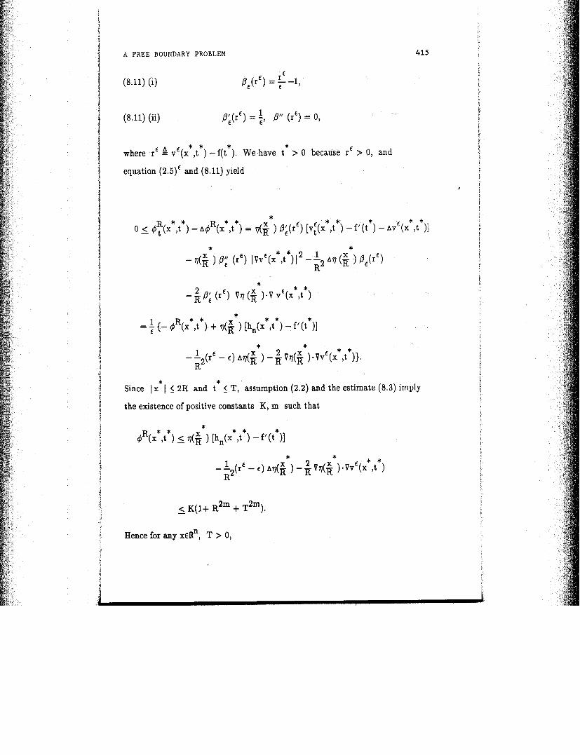
A FREE BOUNDARY PROBLEM
(8.11) (i) PC(r E 1 = 7 r' -1,
1 (8.11) (ii) p;(r') = 7' 8" (r') = 0, i
r
* * I € 4 c * * where r - v (x ,t ) - f(t ). We have t > 0 because r' > 0, and 1
equation (2.5)' and (8.11) yield
* * Since I x I 5 2R and t < T, assumption (2.2) and the estimate (8.3) imply
i the existence of positive constants K, m such that
Hence for any x€IRn, T > 0,
Dow
nloa
ded
by [
ET
H Z
uric
h] a
t 02:
40 1
1 Ju
ne 2
012

416 SONER AND SHREVE
~ ~ ( v ' ( x , T ) -f(T)) = m l x l ( x , ~ ) 5 $IXl(x*,t*) < K (1 + 1 x 1 ~ ~ + TZm).
We obtain (8.9) after observing that AV' = vr + hn + Pa(v'(x,t) - f(t)).
We conclude by proving a comparison result for equation (1.3). A
direct consequence of it, with fl = iRn, is the uniqueness of the polynomially
growing solution to (1.3) and (1.4). The following generality is needed in
Section 4.
Let n be a (possibly unbounded) nonempty domain in iRn.
Lemma 8.5 Suppose that v, 7 satisfy the estimate (2.4) andare almost - evevwhere sub and supersolutions to (1.3) and (1.4) on fl x [O,m). Moreover
cssume that 1 5 7 on Bnx[O,m). Then 1 < 7 on fl x [O,m).
Proof. We regularize v and 7, f i s t . Let t be a Cm, non-negative - function with the properties,
For r > 0, set Xr {(x,t) E x [ ~ p ) : distance (x,BR) > a) , and for
(x,t) E C E , define
Dow
nloa
ded
by [
ET
H Z
uric
h] a
t 02:
40 1
1 Ju
ne 2
012

A FREE BOUNDARY PROBLEM 41 7
hi(x,t) J hn(x-cy, t-6s) E(y,s) dy ds.
I s l + l ~ l s l
It is well known that - v' and V ' are infinitely differentiable, and converge
to 1 and V, respectively, as c tends to zero. Moreover, is a
subsolution to
and 7 ' is a supersolution to a related equation (8.15), which we now
derive.
Let G be a compact subset of 0 such that G x 16 ,m) c C'. For
T > 0, set
Now suppose that
for some (x0,t0) E G x [€,TI. Then the definitions of 7 ' and a (G,E,T)
imply that V(x,t) c f(t) whenever I x-xol + I t-to 1 < 6 , and consequently
Dow
nloa
ded
by [
ET
H Z
uric
h] a
t 02:
40 1
1 Ju
ne 2
012

418 SONER AND SHREVE
& v (x,t) - n ~ ( x , t ) 1 hn(x,t) a.e. lx-x0l + 1 t-to[ 5 6 .
Multiplying the above inequality by ( and integrating, we obtain
(8.14) a a V 6 (x0,to) - A 7 '(xo,to) 1 h i (xO,tO).
Recall that we assumed (8.13) to arrive at (8.14). Hence,
a - € (8.15) m a d a v (x,t)- AV '(x,t)- h i (x,t), 7 '(x,t) -(f(t)- E(~(G,E,T))}L 0
V (x,t) E G x[c,T].
It is not difficult to construct a Cm function q satisfying
(8.16) (i) 4 x 1
0 < d x ) 5 e V x E R",
(8.16) (ii) IVV(X)I + I A V ( X ) ~ 5 3 V(X) V X E [Rn.
In fact, a mollification of $( 1 x 1 ) will work, where
Consider the auxiliary function
Dow
nloa
ded
by [
ET
H Z
uric
h] a
t 02:
40 1
1 Ju
ne 2
012

A FREE BOUNDARY PROBLEM
Since 1 and f are polynomially growing, cp achieves its maximum over
a x [Op) at some (x0,t0). If to = 0 or xo E %I, then
from which follows 1 < f. We assume therefore that xo E fl and to > 0.
For r > 0, 6 2 0, define the smooth function
1 Set ro = minjdistance (xo, %I), to}. Then for fixed 6 > 0, there is an * *
s E (O,ro) such that V r E (0,r ), there exist (x,,t ,), depending on 6, and
satisfying Ix,-xol + I tr-to/ < to,
* Note that (xr,t r) E E c BE for all r E ( 0 , ~ ~ ) . Hence, for all r E (0,a ),
€0
where G = {x : Ix-xo/ < rO} and T = to + rO.
Continuing to hold 6 fixed, we let E 1 0 along a subsequence so that * * * *
(xr,t ,) converges to a limit (x ,t ) satisfying Ix -xO I + ( t -tO1 5 rO. But
Dow
nloa
ded
by [
ET
H Z
uric
h] a
t 02:
40 1
1 Ju
ne 2
012

420 SONER AND SHREVE
* * * 2 * 2 ID(x ,t )-6(1x -xOI t It -tOl ) = limp'16(xc,tE)
€1 0
* * SO x = xo, t = t 0' It follows that l i m (xt,tc) = (x0,t0), where the limit
* €1 0 is taken over all 6 E ( 0 , ~ ).
If Y ' ( X ~ , ~ €) 2 f(t t ) - ea(G,c,T), then (8.18) implies that
vc16(x,,t,) ra(G,r,T)q(xE) + fC(tc) -f(tE). Letting first e 1 0 and then
6 1 0, we obtain (8.17) and conclude as before that y 5 V.
It remains to examine the case
- (8.20) v '(xc,tf) < f ( t f ) - c a(G, c , T).
Because has a local maximum at (xc,t,), we have
€ Vrltx,) -2[V y (x,, t J - v v ,(x,, tc)]. } + 26(n+to - t,) 7 x c
Dow
nloa
ded
by [
ET
H Z
uric
h] a
t 02:
40 1
1 Ju
ne 2
012

A FREE BOUNDARY PROBLEM
where we have used (8.18) - (8.20) to obtain the last inequality. Also,
€ 6 (8.22) 0 = V cp ' (xc,tc) . V7(xc)
-20t = e n(x6) { [V xyr(xE, t J - v 7 '(xc, tJl V n(x,)
Substitution of (8.22) into (8.21) allows us to eliminate the V - V 7 ' term in the latter equation. We may then invoke the bound (8.16)(ii) to
obtain
Letting first 6 1 0 and then 6 1 0 again yields (8.17). n
Dow
nloa
ded
by [
ET
H Z
uric
h] a
t 02:
40 1
1 Ju
ne 2
012

4 22 SONER AND SHREVE
Proofs of Theorem 2.1 and 2.2.
Estimates (8.6) and (8.9) imply the second-derivative estimate (2.4)
for v', and this estimate is uniform in c . This, together with (8.3), gives
(2.4). Using this estimate we choose a subsequence, denoted by E again,
such that v', VV' converge uniformly on bounded subsets. Let v be the
limit; then v also satisfies (2.4). Moreover, using the weak formulation of
(2.5)', we conclude that the limit v is a solution to (1.3), and trivially to
(1.4). Suppose 7 is another point of the sequence vt as E tends to zero.
Then 7 satisfies (1.3), (1.4) and (2.4). Since there is only one function
(recall Lemma 8.5 with n = IR") satisfying (1.3), (1.4) and (2.4), v = v.
Hence v' converges to the unique solution v on the whole sequence. o
Footnotes
Work supported by the National Science Foundation under grants DMS-8742537, and DMS-9042249.
Work supported by the Air Force Office of Scientific Research under grant AFOSR-894075.
REFERENCES
V. E. Benes, L. A. Shepp and H. S. Witsenhaussen, Some solvable stochastic control problems, Stochastics, 4 (1980), 39-83.
J . A. Bather and H. Chernoff, Sequential decisions in the control of a spaceship, Proc. Fifth Berkeley Symposium on Math. Statistics and Probability 3 (1966), 181-207.
A. Bensoussan and J . L. Lions, Applications of variational inequalities in stochastic control, North-Holland, Amsterdam, New York, London, (1982).
H. BrCzis and D. Kinderlehrer, The smoothness of solutions to nonlinear variational inequalities, Indiana U. Math. J., 2319 (1974), 831-844.
L. A. Cafarelli, The regularity of free boundaries in higher dimensions, Acta Mathematzca, 13914 (1977), 155-184.
Dow
nloa
ded
by [
ET
H Z
uric
h] a
t 02:
40 1
1 Ju
ne 2
012

A FREE BOUNDARY PROBLEM 423
P. L. Chow, J . L. Menaldi, and M. Robin, Additive control of stochastic linear systems with finite horizon, SIAM J. Conti Opt., 23 (1985), 858-899.
N. El Karoui and I. Karatzas, Integration of the optiomal stopping time and a new approach to the Skorokhod problem, preprint.
L. C. Evans, A second order elliptic equation with gradient constraint, Comm. PDE, 415 (1979), 555-572.
A. Friedman, Variational principles and free boundary problems, J. Wiley & Sons, (1982).
A. Friedman and R. Jensen, A parabolic quasi-variational inequality arising in Hydraulics, Annuli Scuola Normale Sup.-Pisa, Serie IV, Vol. 11, n.3, (1975), 421-468.
A. Friedman and D. Kinderlehrer, A one-phase Stefan problem, Indiana Univ. Math. J., 24, (1975), 1005-1035.
J. M. Harrison, Brownian motion and stochastic flow systems, Wiley, New York, (1985).
J . M. Harrison and A. J . Taylor, 0 t i m d control of a Brownian storage system, Sfoch. P roc Appl., (?.978), 179-194.
J . M. Harrison and M. I. Taksar, Instantaneous control of a Brownian motion, Math. Oper. Res., 8 (1983), 439453.
H. Ishii and S. Koike, Boundary regularity and uniqueness for an elliptic equation with gradient constraint, Comm. PDE, 814 (1983), 31 7-346.
I. Karatzas, The monotone follower in stochastic decision theory, Appl. Math. Optim., 7 (1981), 175-189.
I. Karatzas, A class of singular stochastic control problems. Adv. Appl. Prob., 15 (1983), 225-254.
I. Karatzas, Probabilistic aspects of finite-fuel stochastic control, Proc. Nat'l. Acad. Sciences USA 82 (1985)
I. Karatzas and S. E. Shreve, Connections between optimal stopping and singular stochastic control I: Monotone follower p~oblems, SIAM J. Cont. Opt., 22 (1984), 856-877.
D. Kinderlehrer and L. Nirenberg, .Regularity in free boundary problems, Ann. Scuola Norm. Sup. Pisa, Ser. IV 4 (1977), 373-391.
0. A. Ladyzenskaya, V. A. Solonnikov and N. N. Ural'ceva, Linear and Quasi-Linear Equations of Parabolic Type, A.M.S. Translation, (1968), Providence, R.I.
Dow
nloa
ded
by [
ET
H Z
uric
h] a
t 02:
40 1
1 Ju
ne 2
012

SONER AND SHREVE
J. L. Menaldi and M. Robin, On some cheap control problems for diffusion process, Transactions of A. M.S., 27812, (1983), 771-802.
J. L. Menaldi and M. I. Taksar, Optimal correction problem of a multidimensional stochastic system, Autornatica, 2512 (1989), 223-232.
P. A. Mevers. Lecture Notes in Mathematics 511, Seminaire de roba abilities X, Universite de Strasbourg, springer-verlag, New York, (1976).
S. Shreve, An introduction to singular stochastic cntrol, in Stochastic Differential Systems, Stochastic Control Theory and Applications, IMA Vol. 10, W. Fleming and P. -L. Lions, ed. Springer-Verlag, New York, 1988.
S. E. Shreve, 3. P. Lehoczky and D. P. Gaver, Optimal consumption for general diffusions with absorbing and reflecting barriers, SIAM J. Cod. Opt. 22 (1984), 55-79.
S. E. Shreve and H. M. Soner, A free boundary problem related to singular stochastic control, Proceedings of Imperial College Workshop on Applied Stochastic Analysis, M. H. A. Davis, ed., (in press).
H. M. Soner and S. E. Shreve, Regularity of the value function for a two-dimensional singular stochastic control problem, SIAM J. Cont. Opt., 27 (1989), 876-907.
P. L. J. Van Moerbeke, An optimal stopping problem with linear reward, Acta Mathernatica, 1-2, 132 (1974), 539-578.
P. L. J. Van Moerbeke, On optimal stop ing and free boundary problems, Arc. R a t Mec. An., 6012 (19765, 101-148.
Received March 1990
Revised October 1990
Dow
nloa
ded
by [
ET
H Z
uric
h] a
t 02:
40 1
1 Ju
ne 2
012