www.pythian.com | White Paper 1

The purpose of this document is to provide a framework and help guide you through

the process of migrating a data warehouse to Google BigQuery. It highlights many

of the areas you should consider when planning for and implementing a migration

of this nature, and includes an example of a migration from another cloud data

warehouse to BigQuery. It also outlines some of the important differences between

BigQuery and other database solutions, and addresses the most frequently asked

questions about migrating to this powerful database.

Note: This document does not claim to provide any benchmarking or performance

comparisons between platforms, but rather highlights areas and scenarios where

BigQuery is the best option.

A FRAMEWORK FOR MIGRATING YOUR DATA WAREHOUSE TO GOOGLE BIGQUERY Vladimir StoyakPrincipal Consultant for Big Data, Certified Google Cloud Platform Qualified Developer

www.pythian.com | White Paper 2

TABLE OF CONTENTSPRE-MIGRATION 3

MAIN MOTIVATORS 3

DEFINING MEASURABLE MIGRATION GOALS 4

PERFORMANCE 4

INFRASTRUCTURE, LICENSE AND MAINTENANCE COSTS 5

USABILITY AND FUNCTIONALITY 5

DATABASE MODEL REVIEW AND ADJUSTMENTS 6

DATA TRANSFORMATION 7

CONTINUOUS DATA INGESTION 7

REPORTING, ANALYTICS AND BI TOOLSET 8

CAPACITY PLANNING 8

MIGRATION 8

STAGING REDSHIFT DATA IN S3 9

REDSHIFT CLI CLIENT INSTALL 9

TRANSFERRING DATA TO GOOGLE CLOUD STORAGE 9

DATA LOAD 10

ORIGINAL STAR SCHEMA MODEL 11

BIG FAT TABLE 13

DATE PARTITIONED FACT TABLE 15

DIMENSION TABLES 17

SLOWLY CHANGING DIMENSIONS (SCD) 17

FAST CHANGING DIMENSIONS (FCD) 18

POST-MIGRATION 18

MONITORING 18

STACKDRIVER 18

AUDIT LOGS 19

QUERY EXPLAIN PLAN 20

www.pythian.com | White Paper 3

PRE-MIGRATION MAIN MOTIVATORSHaving a clear understanding of main motivators for the migration will help

structure the project, set priorities and migration goals, and provide a basis for

assessing the success of the project at the end.

Google BigQuery is a lightning-fast analytics database. Customers find BigQuery’s

performance liberating, allowing them to experiment with enormous datasets

without compromise and to build complex analytics applications such as reporting

and data warehousing.

Here are some of the main reasons that users find migrating to BigQuery an

attractive option:

• BigQuery is a fully managed, no-operations data warehouse. The concept of

hardware is completely abstracted away from the user.

• BigQuery enables extremely fast analytics on a petabyte scale through its

unique architecture and capabilities.

• BigQuery eliminates the need to forecast and provision storage and

compute resources in advance. All the resources are allocated dynamically

based on usage.

• BigQuery provides a unique ‘pay as you go’ model for your data warehouse

and allows you to move away from a CAPEX-based model.

• BigQuery charges separately for data storage and query processing

enabling an optimal cost model, unlike solutions where processing capacity

is allocated (and charged) as a function of allocated storage.

• BigQuery employs a columnar data store, which enables the highest data

compression and minimizes data scanning in common data warehouse

deployments.

• BigQuery provides support for streaming data ingestions directly through an

API or by using Google Cloud Dataflow.

• BigQuery has native integrations with many third-party reporting and BI

providers such as Tableau, MicroStrategy, Looker, and so on.

And some scenarios where BigQuery might not be a good fit:

• BigQuery is not an OLTP database. It performs full column scans for all columns

in the context of the query. It can be very expensive to perform a single row read

similar to primary key access in relational databases with BigQuery.

• BigQuery was not built to be a transactional store. If you are looking to implement

locking, multi-row/table transactions, BigQuery may not be the right platform.

www.pythian.com | White Paper 4

• BigQuery does not support primary keys and referential integrity. During the

migration the data model should be flattened out and denormalized before

storing it in BigQuery to take full advantage of the engine.

• BigQuery is a massively scalable distributed analytics engine where querying

smaller datasets is overkill because in these cases, you cannot take full

advantage of its highly distributed computational and I/O resources.

DEFINING MEASURABLE MIGRATION GOALSBefore an actual migration to BigQuery most companies will identify a “lighthouse

project” and build a proof of concept (PoC) around BigQuery to demonstrate its

value. Explicit success criteria and clearly measurable goals have to be defined

at the very beginning, even if it’s only a PoC of a full-blown production system

implementation. It’s easy to formulate such goals generically for a production

migration as something like: “to have a new system that is equal to or exceeds

performance and scale of the current system and costs less”. But it’s better to

be more specific. PoC projects are smaller in scope so they require very specific

success criteria.

As a guideline, measurable metrics in at least the following three categories have

to be established and observed throughout the migration process: performance,

infrastructure/license/maintenance costs, and usability/functionality.

PERFORMANCE

In an analytical context, performance has a direct effect on productivity, because

running a query for hours means days of iterations between business questions.

It is important to build a solution that scales well not only in terms of data volume

but, in the quantity and complexity of the queries performed.

For queries, BigQuery uses the notion of ‘slots’ to allocate query resources during

query execution. A ‘slot’ is simply a unit of analytical computation (i.e. a chunk of

infrastructure) pertaining to a certain amount of CPU and RAM. All projects, by

default, are allocated 2,000 slots on a best effort basis. As the use of BigQuery

and the consumption of the service goes up, the allocation limit is dynamically

raised. This method serves most customers very well, but in rare cases where a

higher number of slots is required, or/and reserved slots are needed due to strict

SLAs, a new flat-rate billing model might be a better option as it allows you to

choose the specific slot allocation required.

To monitor slot usage per project, use BigQuery integration with Stackdriver. This

captures slot availability and allocations over time for each project. However, there

is no easy way to look at resource usage on a per query basis. To measure per

query usage and identify problematic loads, you might need to cross-reference

slot usage metrics with the query history and query execution.

www.pythian.com | White Paper 5

INFRASTRUCTURE, LICENSE AND MAINTENANCE COSTS

In the case of BigQuery, Google provides a fully managed serverless platform that

eliminates hardware, software and maintenance costs as well as efforts spent on

detailed capacity planning thanks to embedded scalability and a utility billing model -

services are billed based on the volume of data stored and amount of data processed.

It is important to pay attention to the following specifics of BigQuery billing:

• Storage is billed separately from processing so working with large amounts

of “cold” data (rarely accessed) is very affordable.

• Automatic pricing tiers for storage (short term and long term) eliminate the need

of commitment to and planning for volume discounts – they are automatic.

• Processing cost is ONLY for data scanned, so selecting the minimum amount

of columns required to produce results will minimize the processing costs

thanks to columnar storage. This is why explicitly selecting required columns

instead of “*” can make a big processing cost (and performance) difference.

• Likewise, implementing appropriate partitioning techniques in BigQuery will

result in less data scanned and lower processing costs (in addition to better

performance). This is especially important since BigQuery doesn’t utilize the

concept of indexes that’s common to relational databases.

• There is an extra charge if a streaming API is used to ingest data into

BigQuery in real time.

• Cost control tools such as “Billing Alerts” and “Custom Quotas” and alerting

or limiting resource usage per project or user might come in handy (https://

cloud.google.com/bigquery/cost-controls)

Learning from early adoption, in addition to usage-based billing, Google is

introducing a new pricing model where customers can choose a fixed billing

model for data processing. And, although it seems like usage-based billing

might still be a better option for most of the use cases and clients, receiving a

predictable bill at the end of the month is attractive to some organizations.

USABILITY AND FUNCTIONALITY

There may be some functional differences when migrating to a different platform,

however in many cases there are workarounds and specific design considerations

that can be adopted to address these.

BigQuery launched support for standard SQL, which is compliant with the SQL 2011

standard and has extensions that support querying nested and repeated data.

www.pythian.com | White Paper 6

It is worth exploring some additional SQL language/engine specifics and some

additional functions:

• Analytic/window functions

• JSON parsing

• Working with arrays

• Correlated subqueries

• Temporary SQL/Javascript user defined functions

• Inequality predicates in joins

• Table name wildcards and table suffixes

In addition, BigQuery support for querying data directly from Google Cloud

Storage and Google Drive. It supports AVRO, JSON NL, CSV files as well as

Google Cloud Datastore backup, Google Sheets (first tab only). Federated

datasources should be considered in the following cases:

• Loading and cleaning your data in one pass by querying the data from a

federated data source (a location external to BigQuery) and writing the

cleaned result into BigQuery storage.

• Having a small amount of frequently changing data that you join with other

tables. As a federated data source, the frequently changing data does not

need to be reloaded every time it is updated.

DATABASE MODEL REVIEW AND ADJUSTMENTSIt’s important to remember that a “lift and shift” approach prioritizes ease and speed

of migration over long-term performance and maintainability benefits. This can be

a valid approach if it’s an organization’s priority and incremental improvements can

be applied over time. However, it might not be optimal from a performance and cost

standpoint. ROI on optimization efforts can be almost immediate. In many cases data

model adjustments have to be made to some degree.

While migrating to BigQuery the following are worthwhile considering:

• Limiting the number of columns in the context of the query and specifically

avoid things like “select * from table”.

• Limiting complexity of joins, especially with high cardinality join keys. Some

extra denormalization might come in handy and greatly improve query

performance with minimal impact on storage cost and changes required to

implement them.

• Making use of structured data types.

• Introducing table decorators, table name filters in queries and structuring

data around manual or automated date partitioning.

www.pythian.com | White Paper 7

• Making use of retention policies on Dataset level or set partition expiration

date -time_partitioning_expiration flag.

• Batching DML statements like insert,update and delete.

• Limiting data scanned through use of partitioning (there is only date partition

supported at the moment but multiple tables and table name selectors can

somewhat overcome this limitation).

DATA TRANSFORMATIONExporting data from the source system into a flat file and then loading it into

BigQuery might not always work. In some cases the transformation process

should take place before loading data into BigQuery due to some data type

constraints, changes in data model, etc. For example, WebUI does not allow any

parsing (i.e. date string format), type casting, etc. and source data should be fully

compatible with target schema.

If any transformation is required, the data can potentially be loaded into a

temporary staging table in BigQuery with subsequent processing steps that

would take staged data, and transform/parse it using built-in functions or custom

JavaScript UDFs and loaded it into target schema.

If more complex transformations are required, Google Cloud Dataflow (https://

cloud.google.com/dataflow/) or Google Dataproc (https://cloud.google.com/

dataproc/) can be used as an alternative to custom coding. Here is a good tutorial

demonstrating how to use Google Cloud Dataflow to analyze logs collected and

exported by Google Cloud Logging.

CONTINUOUS DATA INGESTIONInitial data migration is not the only process. And once the migration is completed,

changes will have to be made in the data ingestion process for new data to flow

into the new system. Having a clear understanding of how the data ingestion

process is currently implemented and how to make it work in a new environment is

one of the important planning aspects.

When considering loading data to BigQuery, there are a few options available:

• Bulk loading from AVRO/JSON/CSV on GCS. There are some difference of

what format is best for what, more information available from (https://cloud.

google.com/bigquery/loading-data)

• Using the BigQuery API (https://cloud.google.com/bigquery/loading-data-

post-request)

• Streaming Data into BigQuery using one of the API Client Libraries or

Google Cloud Dataflow

www.pythian.com | White Paper 8

• Using BigQuery to load uncompressed files. This is significantly faster

than compressed files due to parallel load operations, but because

uncompressed files are larger in size, using them can lead to bandwidth

limitations and higher storage costs.

• Loading Avro file, which does not require you to manually define schemas.

The schema will be inherited from the datafile itself.

REPORTING, ANALYTICS AND BI TOOLSETReporting, visualization and BI platform investments in general are significant.

Although some improvements might be needed to avoid bringing additional

dependencies and risks into the migration project (BI/ETL tools replacement),

keeping existing end user tools is a common preference.

There is a growing list of vendors that provide native connection to BigQuery

(https://cloud.google.com/bigquery/partners/). However if native support is not

yet available for for the BI layer in use, then some third-party connectors (such as

Simba https://cloud.google.com/bigquery/partners/simba-beta-drivers in Beta)

might be required as there is no native ODBC/JDBC support yet.

CAPACITY PLANNING

Identifying queries, concurrent users, data volumes processed, and usage pattern

is important to understand. Normally migrations start from identifying and building

a PoC from the most demanding area where the impact will be well visible.

As access to big data is being democratized with better user interfaces, standard

SQL support and faster queries, it makes the reporting/data mining self-serviced

and variability of analysis much wider. This shifts the attention from boring

administrative and maintenance tasks to what really matters to the business:

generating insights and intelligence from the data. As a result, the focus for

organizations is in expanding capacity in business analysis, developing expertise

in data modeling, data science, machine learning and statistics, etc.

BigQuery removes the need for capacity planning in most cases. Storage is

virtually infinitely scalable and data processing compute capacity allocation is

done automatically by the platform as data volumes and usage grow.

MIGRATIONTo test a simple “Star Schema” to BigQuery migration scenario we will be loading

a SSB sample schema into Redshift and then performing ETL into BigQuery.

This schema was generated based on the TPC-H benchmark with some data

warehouse specific adjustments.

www.pythian.com | White Paper 9

REDSHIFT CLI CLIENT INSTALL

In order not to depend on a connection with a local workstation while loading

data, an EC2 micro instance was launched so we could perform data load steps

described in http://snowplowanalytics.com/blog/2013/02/20/transferring-data-

from-s3-to-redshift-at-the-command-line/

We also needed to download the client from http://www.xigole.com/software/jisql/

build/jisql-2.0.11.zip

The client requires the following environment variables to store AWS access

credentials

• export ACCESS-KEY=

• export SECRET-ACCESS-KEY=

• export USERNAME=

• export PASSWORD=

Once RedShift CLI client is installed and access credentials are specified, we need to

• create source schema in RedShift

• load SSB data into RedShift

• Export data to S3

Here are some of the files and scripts needed

https://gist.github.com/anonymous/657b5175b978cdc7dd0cba2b0d44ef77

After executing the scripts in the above link, you will have an export of your

Redshift tables in S3.

TRANSFERRING DATA TO GOOGLE CLOUD STORAGEOnce the export is created you can use GCP Storage Transfer utility to move files

from S3 to Cloud Storage (https://cloud.google.com/storage/transfer/). In addition

to WebUI you can create and initiate transfer using Google API Client library for

the language of your choice or REST API. If you are transferring less than 1TB of

data then the gsutil command-line tool can also be used to transfer data between

Cloud Storage and other locations.

Cloud Storage Transfer Service has options that make data transfers and

synchronization between data sources and data sinks easier.

For example, you can:

• Schedule one-time transfers or recurring transfers.

• Schedule periodic synchronization from data source to data sink with

STAGING REDSHIFT DATA IN S3

www.pythian.com | White Paper 10

advanced filters based on file creation dates, file-name filters, and the times

of day you prefer to import data.

• Delete source objects after transferring them.

For subsequent data synchronizations, data should ideally be pushed directly from

the source into GCP. If for legacy reasons data must be staged in AWS S3 the

following approaches can be used to load data into BigQuery on an ongoing basis

assuming:

• Policy on S3 bucket is set to create a SQS message on object creation.

In GCP we can use Dataflow and create custom unbounded source to

subscribe to SQS messages and read and stream newly created objects into

BigQuery

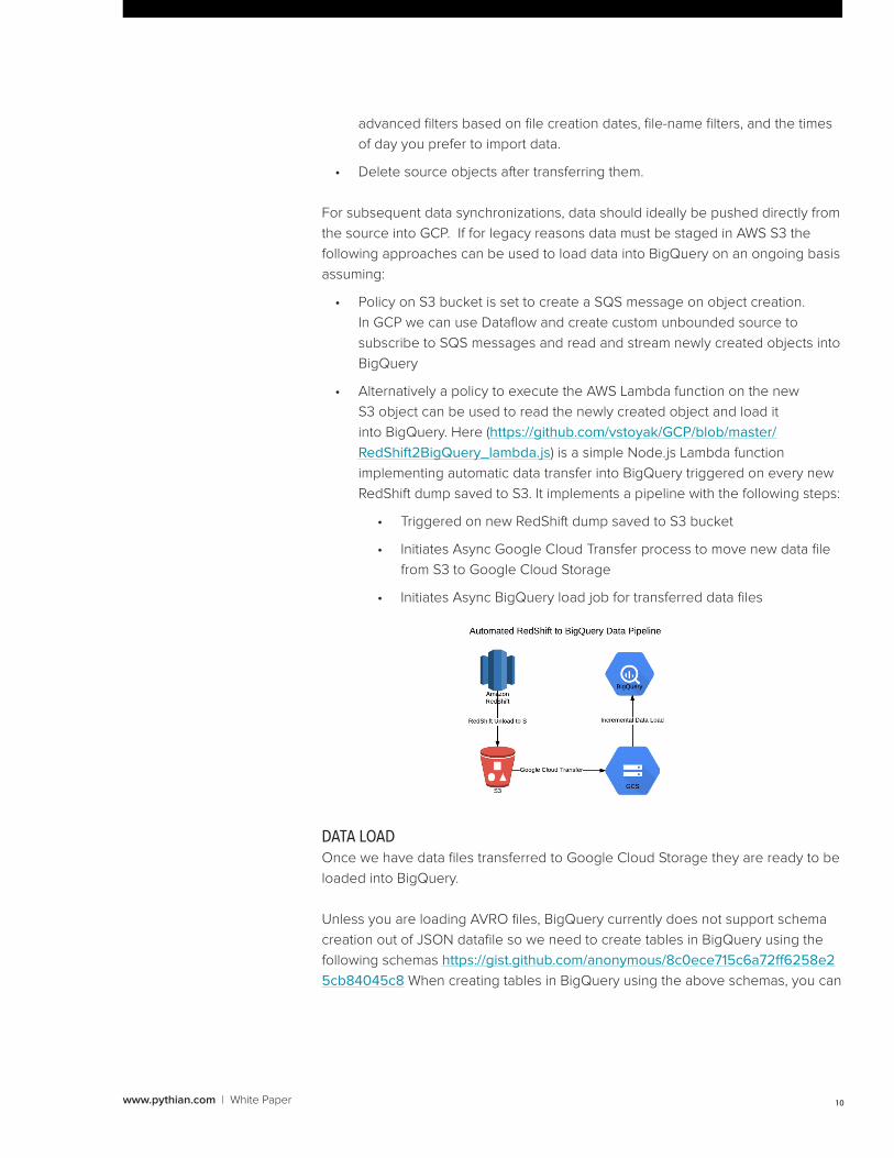
• Alternatively a policy to execute the AWS Lambda function on the new

S3 object can be used to read the newly created object and load it

into BigQuery. Here (https://github.com/vstoyak/GCP/blob/master/

RedShift2BigQuery_lambda.js) is a simple Node.js Lambda function

implementing automatic data transfer into BigQuery triggered on every new

RedShift dump saved to S3. It implements a pipeline with the following steps:

• Triggered on new RedShift dump saved to S3 bucket

• Initiates Async Google Cloud Transfer process to move new data file

from S3 to Google Cloud Storage

• Initiates Async BigQuery load job for transferred data files

DATA LOADOnce we have data files transferred to Google Cloud Storage they are ready to be

loaded into BigQuery.

Unless you are loading AVRO files, BigQuery currently does not support schema

creation out of JSON datafile so we need to create tables in BigQuery using the

following schemas https://gist.github.com/anonymous/8c0ece715c6a72ff6258e2

5cb84045c8 When creating tables in BigQuery using the above schemas, you can

www.pythian.com | White Paper 11

load data at the same time. To do so you need to point the BigQuery import tool

to the location of datafiles on Cloud Storage. Please note that since there will be

multiple files created for each table when exporting from RedShift, you will need to

specify wildcards when pointing to the location of corresponding datafiles.

One caveat here is that BigQuery data load interfaces are rather strict in what

formats they accept and unless all types are fully compatible, properly quoted

and formatted, the load job will fail with very little indication as to where the

problematic row/column is in the source file.

There is always an option to load all fields as STRING and then do the

transformation into target tables using default or user defined functions. Another

approach would be to rely on Google Cloud Dataflow (https://cloud.google.com/

dataflow/) for the transformation or ETL tools such as Talend or Informatica.

For help with automation of data migration from RedShift to BigQuery you can

also look at BigShift utility (https://github.com/iconara/bigshift). BigShift follows the

same steps dumping RedShift tables into S3, moving them over to Google Cloud

Storage and then loading them into BigQuery. In addition, it implements automatic

schema creation on the BigQuery side and implements type conversion, cleansing

in case the source data does not fit perfectly into formats required by BigQuery

(data type translation, timestamp reformatting, quotes are escaped, and so on). You

should review and evaluate the limitations of BigShift before using the software

and make sure it fits what you need.

ORIGINAL STAR SCHEMA MODELWe have now loaded data from RedShift using a simple “lift & shift” approach. No

changes are really required and you can start querying and joining tables “as-is” using

Standard SQL. Query optimizer will insure that the query is executed in most optimal

stages, but you have to ensure that “Legacy SQL” is unchecked in Query Options.

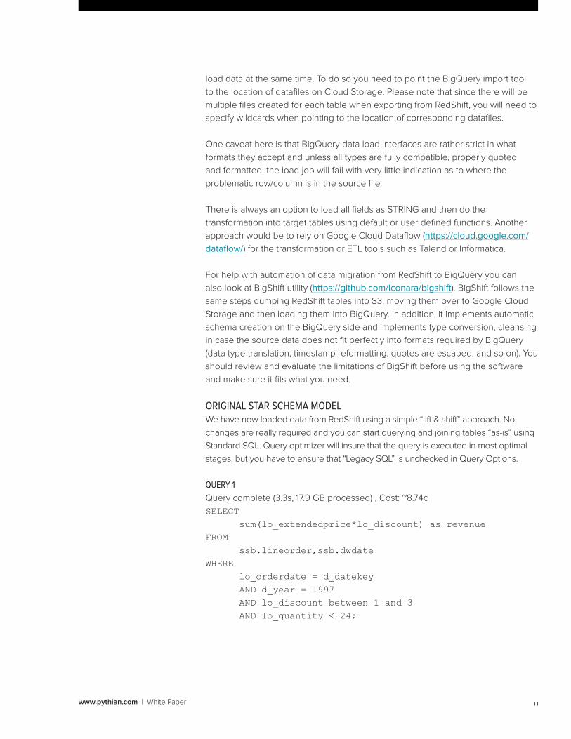
QUERY 1

Query complete (3.3s, 17.9 GB processed) , Cost: ~8.74¢

SELECT sum(lo_extendedprice*lo_discount) as revenue

FROMssb.lineorder,ssb.dwdate

WHERE lo_orderdate = d_datekeyAND d_year = 1997 AND lo_discount between 1 and 3 AND lo_quantity < 24;

www.pythian.com | White Paper 12

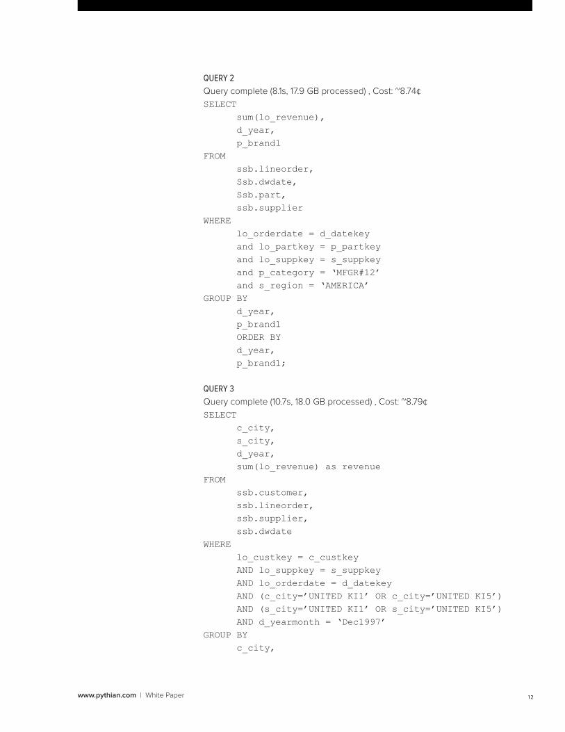
QUERY 2

Query complete (8.1s, 17.9 GB processed) , Cost: ~8.74¢

SELECT sum(lo_revenue), d_year, p_brand1

FROMssb.lineorder,Ssb.dwdate,Ssb.part,ssb.supplier

WHERE lo_orderdate = d_datekeyand lo_partkey = p_partkeyand lo_suppkey = s_suppkeyand p_category = ‘MFGR#12’and s_region = ‘AMERICA’

GROUP BYd_year,p_brand1ORDER BY d_year,p_brand1;

QUERY 3

Query complete (10.7s, 18.0 GB processed) , Cost: ~8.79¢

SELECT c_city, s_city, d_year, sum(lo_revenue) as revenue

FROMssb.customer,ssb.lineorder,ssb.supplier,ssb.dwdate

WHERElo_custkey = c_custkeyAND lo_suppkey = s_suppkeyAND lo_orderdate = d_datekeyAND (c_city=’UNITED KI1’ OR c_city=’UNITED KI5’)AND (s_city=’UNITED KI1’ OR s_city=’UNITED KI5’)AND d_yearmonth = ‘Dec1997’

GROUP BYc_city,

www.pythian.com | White Paper 13

S_city,d_year

ORDER BY d_year ASCrevenue DESC;

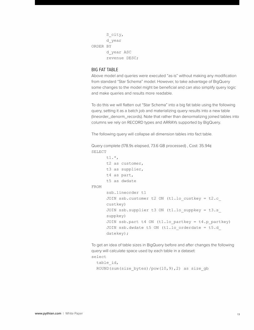
BIG FAT TABLEAbove model and queries were executed “as-is” without making any modification

from standard “Star Schema” model. However, to take advantage of BigQuery

some changes to the model might be beneficial and can also simplify query logic

and make queries and results more readable.

To do this we will flatten out “Star Schema” into a big fat table using the following

query, setting it as a batch job and materializing query results into a new table

(lineorder_denorm_records). Note that rather than denormalizing joined tables into

columns we rely on RECORD types and ARRAYs supported by BigQuery.

The following query will collapse all dimension tables into fact table.

Query complete (178.9s elapsed, 73.6 GB processed) , Cost: 35.94¢

SELECTt1.*, t2 as customer, t3 as supplier, t4 as part, t5 as dwdate

FROM ssb.lineorder t1 JOIN ssb.customer t2 ON (t1.lo_custkey = t2.c_custkey)JOIN ssb.supplier t3 ON (t1.lo_suppkey = t3.s_suppkey)JOIN ssb.part t4 ON (t1.lo_partkey = t4.p_partkey)JOIN ssb.dwdate t5 ON (t1.lo_orderdate = t5.d_datekey);

To get an idea of table sizes in BigQuery before and after changes the following

query will calculate space used by each table in a dataset:

select table_id, ROUND(sum(size_bytes)/pow(10,9),2) as size_gb

www.pythian.com | White Paper 14

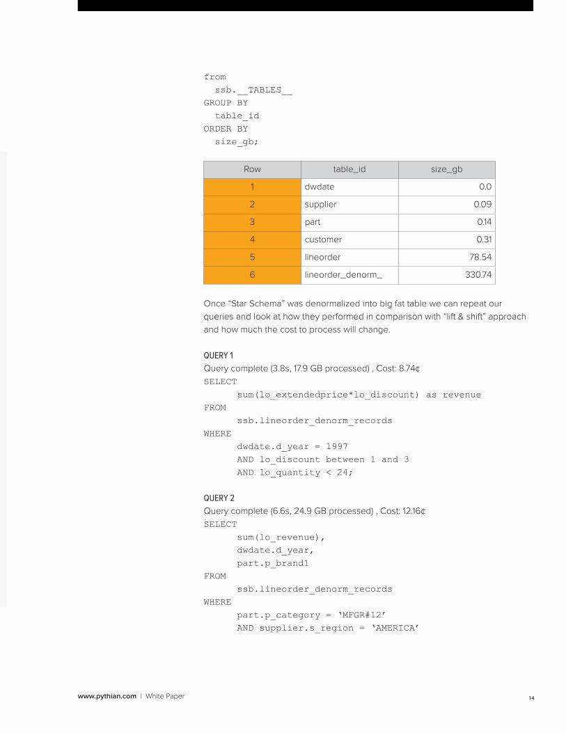
from ssb.__TABLES__GROUP BY table_idORDER BY size_gb;

Row table_id size_gb

1 dwdate 0.0

2 supplier 0.09

3 part 0.14

4 customer 0.31

5 lineorder 78.54

6 lineorder_denorm_ 330.74

Once “Star Schema” was denormalized into big fat table we can repeat our

queries and look at how they performed in comparison with “lift & shift” approach

and how much the cost to process will change.

QUERY 1

Query complete (3.8s, 17.9 GB processed) , Cost: 8.74¢

SELECTsum(lo_extendedprice*lo_discount) as revenue

FROMssb.lineorder_denorm_records

WHERE dwdate.d_year = 1997AND lo_discount between 1 and 3AND lo_quantity < 24;

QUERY 2

Query complete (6.6s, 24.9 GB processed) , Cost: 12.16¢

SELECTsum(lo_revenue),dwdate.d_year, part.p_brand1

FROMssb.lineorder_denorm_records

WHEREpart.p_category = ‘MFGR#12’AND supplier.s_region = ‘AMERICA’

www.pythian.com | White Paper 15

GROUP BYdwdate.d_year, part.p_brand1

ORDER BYdwdate.d_year,part.p_brand1;

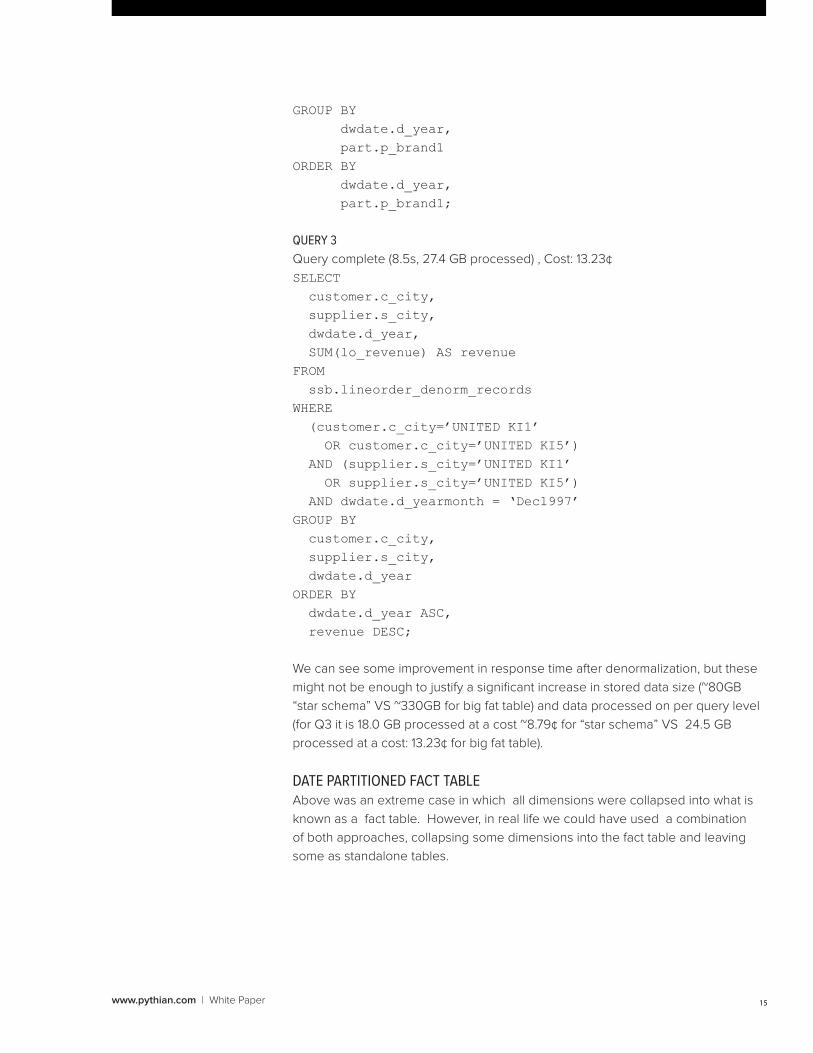
QUERY 3

Query complete (8.5s, 27.4 GB processed) , Cost: 13.23¢

SELECT customer.c_city, supplier.s_city, dwdate.d_year, SUM(lo_revenue) AS revenueFROM ssb.lineorder_denorm_recordsWHERE (customer.c_city=’UNITED KI1’ OR customer.c_city=’UNITED KI5’) AND (supplier.s_city=’UNITED KI1’ OR supplier.s_city=’UNITED KI5’) AND dwdate.d_yearmonth = ‘Dec1997’GROUP BY customer.c_city, supplier.s_city, dwdate.d_yearORDER BY dwdate.d_year ASC, revenue DESC;

We can see some improvement in response time after denormalization, but these

might not be enough to justify a significant increase in stored data size (~80GB

“star schema” VS ~330GB for big fat table) and data processed on per query level

(for Q3 it is 18.0 GB processed at a cost ~8.79¢ for “star schema” VS 24.5 GB

processed at a cost: 13.23¢ for big fat table).

DATE PARTITIONED FACT TABLEAbove was an extreme case in which all dimensions were collapsed into what is

known as a fact table. However, in real life we could have used a combination

of both approaches, collapsing some dimensions into the fact table and leaving

some as standalone tables.

www.pythian.com | White Paper 16

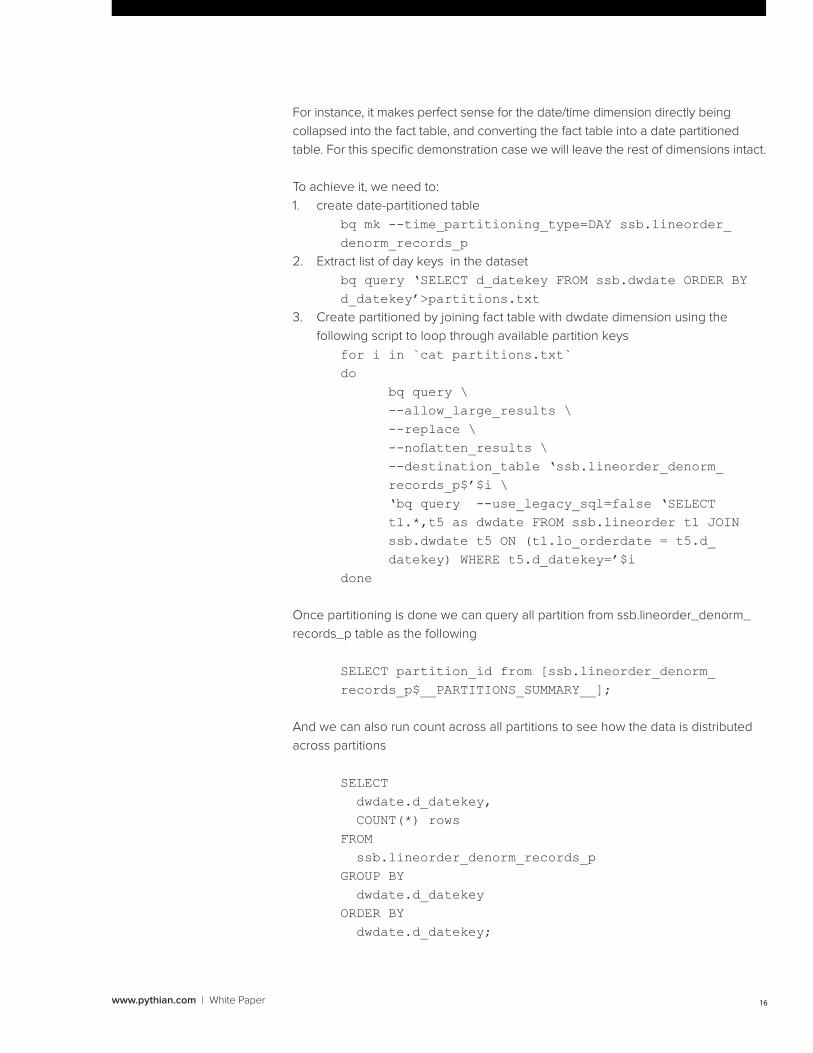
For instance, it makes perfect sense for the date/time dimension directly being

collapsed into the fact table, and converting the fact table into a date partitioned

table. For this specific demonstration case we will leave the rest of dimensions intact.

To achieve it, we need to:

1. create date-partitioned table

bq mk --time_partitioning_type=DAY ssb.lineorder_denorm_records_p

2. Extract list of day keys in the dataset

bq query ‘SELECT d_datekey FROM ssb.dwdate ORDER BY d_datekey’>partitions.txt

3. Create partitioned by joining fact table with dwdate dimension using the

following script to loop through available partition keys

for i in `cat partitions.txt`do bq query \

--allow_large_results \--replace \--noflatten_results \--destination_table ‘ssb.lineorder_denorm_records_p$’$i \‘bq query --use_legacy_sql=false ‘SELECT t1.*,t5 as dwdate FROM ssb.lineorder t1 JOIN ssb.dwdate t5 ON (t1.lo_orderdate = t5.d_datekey) WHERE t5.d_datekey=’$i

done

Once partitioning is done we can query all partition from ssb.lineorder_denorm_

records_p table as the following

SELECT partition_id from [ssb.lineorder_denorm_records_p$__PARTITIONS_SUMMARY__];

And we can also run count across all partitions to see how the data is distributed

across partitions

SELECT dwdate.d_datekey, COUNT(*) rowsFROM ssb.lineorder_denorm_records_pGROUP BY dwdate.d_datekeyORDER BY dwdate.d_datekey;

www.pythian.com | White Paper 17

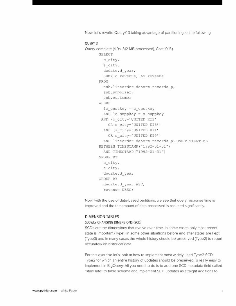
Now, let’s rewrite Query# 3 taking advantage of partitioning as the following

QUERY 3

Query complete (4.9s, 312 MB processed), Cost: 0.15¢

SELECT c_city, s_city, dwdate.d_year, SUM(lo_revenue) AS revenueFROM ssb.lineorder_denorm_records_p, ssb.supplier, ssb.customerWHERE lo_custkey = c_custkey AND lo_suppkey = s_suppkey AND (c_city=’UNITED KI1’ OR c_city=’UNITED KI5’) AND (s_city=’UNITED KI1’ OR s_city=’UNITED KI5’) AND lineorder_denorm_records_p._PARTITIONTIME BETWEEN TIMESTAMP(“1992-01-01”) AND TIMESTAMP(“1992-01-31”)GROUP BY c_city, s_city, dwdate.d_yearORDER BY dwdate.d_year ASC, revenue DESC;

Now, with the use of date-based partitions, we see that query response time is

improved and the the amount of data processed is reduced significantly.

DIMENSION TABLESSLOWLY CHANGING DIMENSIONS (SCD)

SCDs are the dimensions that evolve over time. In some cases only most recent

state is important (Type1) in some other situations before and after states are kept

(Type3) and in many cases the whole history should be preserved (Type2) to report

accurately on historical data.

For this exercise let’s look at how to implement most widely used Type2 SCD.

Type2 for which an entire history of updates should be preserved, is really easy to

implement in BigQuery. All you need to do is to add one SCD metadata field called

“startDate” to table schema and implement SCD updates as straight additions to

www.pythian.com | White Paper 18

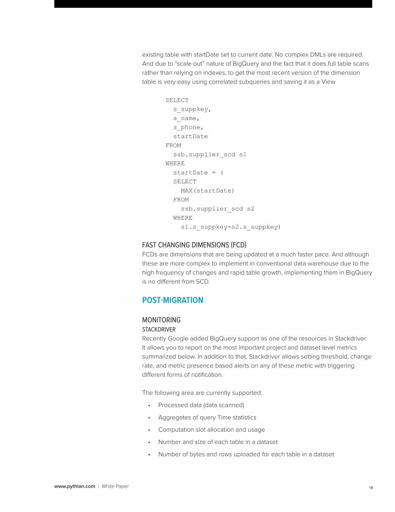
existing table with startDate set to current date. No complex DMLs are required.

And due to “scale out” nature of BigQuery and the fact that it does full table scans

rather than relying on indexes, to get the most recent version of the dimension

table is very easy using correlated subqueries and saving it as a View

SELECT s_suppkey, s_name, s_phone, startDateFROM ssb.supplier_scd s1WHERE startDate = ( SELECT MAX(startDate) FROM ssb.supplier_scd s2 WHERE s1.s_suppkey=s2.s_suppkey)

FAST CHANGING DIMENSIONS (FCD)FCDs are dimensions that are being updated at a much faster pace. And although

these are more complex to implement in conventional data warehouse due to the

high frequency of changes and rapid table growth, implementing them in BigQuery

is no different from SCD.

POST-MIGRATION

MONITORINGSTACKDRIVER

Recently Google added BigQuery support as one of the resources in Stackdriver.

It allows you to report on the most important project and dataset level metrics

summarized below. In addition to that, Stackdriver allows setting threshold, change

rate, and metric presence based alerts on any of these metric with triggering

different forms of notification.

The following area are currently supported:

• Processed data (data scanned)

• Aggregates of query Time statistics

• Computation slot allocation and usage

• Number and size of each table in a dataset

• Number of bytes and rows uploaded for each table in a dataset

www.pythian.com | White Paper 19

And here are some of the current limitations of Stackdriver integration:

• BigQuery resources are not yet supported by Stackdriver Grouping making it hard

to set threshold based alerts based on custom groupings of BigQuery resources.

• Long Running Query report or similar resources used per query views are

not available from Stackdriver making it harder to troubleshoot, identify

problematic queries and automatically react to them.

• There are Webhooks notifications for BigQuery Alerts in Stackdriver, “Custom

Quotas” and “Billing Alerts” in GCP console, but I have not found an easy

way to implement per-query actions.

• On the Alert side I think it might be useful to be able to send messages to Cloud

Function (although general Webhooks are supported already) and PubSub.

• Streamed data is a billable usage and seeing this stat would be useful.

AUDIT LOGS

Stackdriver integration is extremely valuable to get understanding on per project

BigQuery usage, but many times we need to dig deeper and understand platform

usage on a more granular level such as individual department or user levels.

BigQuery Audit (https://cloud.google.com/bigquery/audit-logs) log is a valuable

source for such information and can answer many questions such as:

• who are the users running the queries

• how much data is being processed per query or by an individual user in a

day or a month.

• what is the cost per department processing data

• what are the long running queries or queries processing too much data

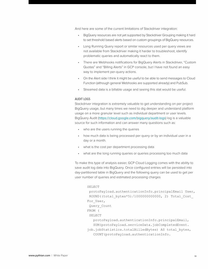
To make this type of analysis easier, GCP Cloud Logging comes with the ability to

save audit log data into BigQuery. Once configured entries will be persisted into

day-partitioned table in BigQuery and the following query can be used to get per

user number of queries and estimated processing charges

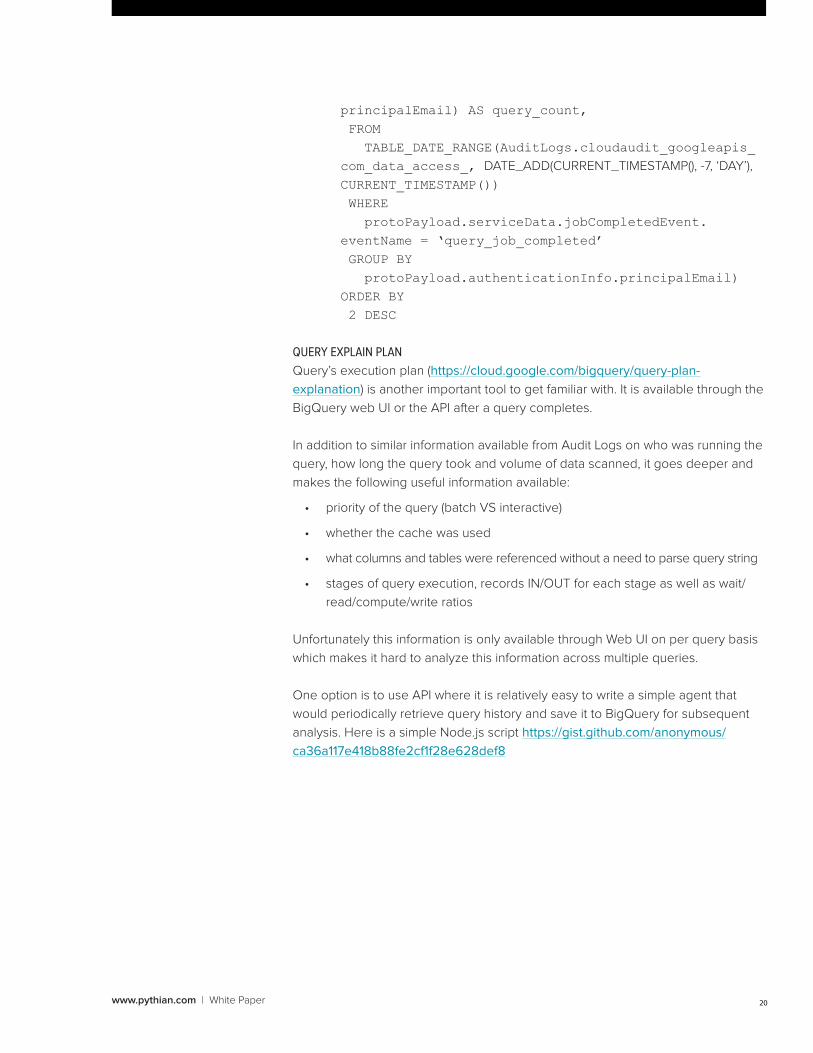
SELECT protoPayload.authenticationInfo.principalEmail User, ROUND((total_bytes*5)/1000000000000, 2) Total_Cost_For_User, Query_CountFROM ( SELECT protoPayload.authenticationInfo.principalEmail, SUM(protoPayload.serviceData.jobCompletedEvent.job.jobStatistics.totalBilledBytes) AS total_bytes, COUNT(protoPayload.authenticationInfo.

www.pythian.com | White Paper 20

principalEmail) AS query_count, FROM TABLE_DATE_RANGE(AuditLogs.cloudaudit_googleapis_com_data_access_, DATE_ADD(CURRENT_TIMESTAMP(), -7, ‘DAY’),

CURRENT_TIMESTAMP()) WHERE protoPayload.serviceData.jobCompletedEvent.eventName = ‘query_job_completed’ GROUP BY protoPayload.authenticationInfo.principalEmail)ORDER BY 2 DESC

QUERY EXPLAIN PLAN

Query’s execution plan (https://cloud.google.com/bigquery/query-plan-

explanation) is another important tool to get familiar with. It is available through the

BigQuery web UI or the API after a query completes.

In addition to similar information available from Audit Logs on who was running the

query, how long the query took and volume of data scanned, it goes deeper and

makes the following useful information available:

• priority of the query (batch VS interactive)

• whether the cache was used

• what columns and tables were referenced without a need to parse query string

• stages of query execution, records IN/OUT for each stage as well as wait/

read/compute/write ratios

Unfortunately this information is only available through Web UI on per query basis

which makes it hard to analyze this information across multiple queries.

One option is to use API where it is relatively easy to write a simple agent that

would periodically retrieve query history and save it to BigQuery for subsequent

analysis. Here is a simple Node.js script https://gist.github.com/anonymous/

ca36a117e418b88fe2cf1f28e628def8

www.pythian.com | White Paper 21

Vladimir Stoyak

Principal Consultant for Big Data, Certified Google Cloud Platform Qualified Developer

Vladimir Stoyak is a principal consultant for big data. Vladimir is a certified Google Cloud Platform

Qualified Developer, and Principal Consultant for Pythian’s Big Data team. He has more than 20 years

of expertise working in Big Data and machine learning technologies including Hadoop, Kafka, Spark,

Flink, Hbase, and Cassandra. Throughout his career in IT, Vladimir has been involved in a number

of startups. He was Director of Application Services for Fusepoint, which was recently acquired by

CenturyLink. He also founded AlmaLOGIC Solutions Incorporated, an e-Learning analytics company.

ABOUT THE AUTHOR

ABOUT PYTHIAN

Pythian is a global IT services company that helps businesses become more competitive by using technology to reach their business goals.

We design, implement, and manage systems that directly contribute to revenue and business success. Our services deliver increased agility

and business velocity through IT transformation, and high system availability and performance through operational excellence. Our highly

skilled technical teams work as an integrated extension of our clients’ organizations to deliver continuous transformation and uninterrupted

operational excellence using our expertise in databases, cloud, DevOps, big data, advanced analytics, and infrastructure management.

V01-092016-NA

Pythian, The Pythian Group, “love your data”, pythian.com, and Adminiscope are trademarks of The Pythian Group Inc. Other product and company names mentioned herein may be trademarks or registered trademarks of their respective owners. The information presented is subject to change without notice. Copyright © <year> The Pythian Group Inc. All rights reserved.

OTHER USEFUL TOOLS

• Streak BigQuery Developer Tools provides graphing, timestamp conversions,

queries across datasets, etc. - https://chrome.google.com/webstore/detail/

streak-bigquery-developer/lfmljmpmipdibdhbmmaadmhpaldcihgd?utm_

source=gmail

• BigQuery Mate provides improvements for BQ WebUI such as cost

estimates, styling, parametarized queries, etc.- https://chrome.google.com/

webstore/detail/bigquery-mate/nepgdloeceldecnoaaegljlichnfognh?u

tm_source=gmail

• Save BigQuery to GitHub - https://chrome.google.com/webstore/detail/save-

bigquery-to-github/heeofgmoliomldhglhlgeikfklacpnad?utm_source=gmail