a framework for life cycle assessment (lca) of emerging

Clemson University Clemson University

TigerPrints TigerPrints

All Dissertations Dissertations

May 2020

A Framework for Life Cycle Assessment (LCA) of Emerging A Framework for Life Cycle Assessment (LCA) of Emerging

Technologies at Low Technology Readiness Levels Technologies at Low Technology Readiness Levels

Sheikh Moniruzzaman Moni Clemson University, [email protected]

Follow this and additional works at: https://tigerprints.clemson.edu/all_dissertations

Recommended Citation Recommended Citation Moni, Sheikh Moniruzzaman, "A Framework for Life Cycle Assessment (LCA) of Emerging Technologies at Low Technology Readiness Levels" (2020). All Dissertations. 2641. https://tigerprints.clemson.edu/all_dissertations/2641

This Dissertation is brought to you for free and open access by the Dissertations at TigerPrints. It has been accepted for inclusion in All Dissertations by an authorized administrator of TigerPrints. For more information, please contact [email protected].

https://tigerprints.clemson.edu/

https://tigerprints.clemson.edu/all_dissertations

https://tigerprints.clemson.edu/dissertations

https://tigerprints.clemson.edu/all_dissertations?utm_source=tigerprints.clemson.edu%2Fall_dissertations%2F2641&utm_medium=PDF&utm_campaign=PDFCoverPages

https://tigerprints.clemson.edu/all_dissertations/2641?utm_source=tigerprints.clemson.edu%2Fall_dissertations%2F2641&utm_medium=PDF&utm_campaign=PDFCoverPages

mailto:[email protected]

A FRAMEWORK FOR LIFE CYCLE ASSESSMENT (LCA) OF EMERGING

TECHNOLOGIES AT LOW TECHNOLOGY READINESS LEVELS

A Dissertation

Presented to

the Graduate School of

Clemson University

In Partial Fulfillment

of the Requirements for the Degree

Doctor of Philosophy

Environmental Engineering and Earth Sciences

by

Sheikh Moniruzzaman Moni

May 2020

Accepted by

Dr. Michael Carbajales-Dale, Committee Co-Chair

Dr. Karen High, Committee Co-Chair

Dr. Terry Walker

Dr. Sudeep Popat

ii

ABSTRACT

In recent literature, prospective application of life cycle assessment (LCA) at low

technology readiness levels (TRL) has gained immense interest for its potential to enable

development of emerging technologies with improved environmental performances.

However, limited data, uncertain functionality, scale-up issues and uncertainties make it

very challenging for the standard LCA guidelines to evaluate emerging technologies and

requires methodological advances in the current LCA framework. In this work, we

describe major methodological challenges and analyzed key research efforts to resolve

these issues with a focus on recent developments in five major areas: cross-study

comparability, data availability and quality, scale-up issues, uncertainty and uncertainty

communication, and assessment time. We develop a novel prospective LCA framework

(LCA-ET) to evaluate emerging technologies at low technology readiness level. We

demonstrate the application of this LCA-ET framework to evaluate two emerging

technologies: (1) perovskite solar photovoltaic module and (2) anaerobic membrane

bioreactor for domestic wastewater treatment. We also provide a number of

recommendations for future research to support the evaluation of emerging technologies

at low technology readiness level: (1) the development of a consistent framework and

reporting methods for LCA of emerging technologies; (2) the integration of other tools

with LCA, such as multicriteria decision analysis, risk analysis, techno-economic

analysis; and (3) the development of a data repository for emerging materials, processes,

and technologies.

iii

DEDICATION

To my family.

iv

ACKNOWLEDGMENTS

I would like to express my sincere gratitude to my both advisors Dr. Michael

Carbajales-Dale and Dr. Karen High for their invaluable guidance, inspiration,

professionalism and patience throughout my PhD program. Despite their busy schedule,

they always managed time to support me with their immense knowledge and endless

encouragement. My sincere appreciation extends to my committee members Dr. Terry

Walker and Dr. Sudeep Popat for their helpful suggestions and technical insights.

Suggestions from Dr. Popat helped me a lot to complete AnMBR case study. Insightful

comments from Dr. Walker on the manuscript was so helpful. I also want to thank Dr.

Amy Landis for her support at the beginning of my PhD study at Clemson University.

Special thanks to Dr. Mizanur Rahman for his encouragement and generous support.

Heartiest gratitude and appreciation to my wife, Roksana Mahmud for her

encouragement, understanding and sacrifice. Without her incredible support, it would not

be possible to complete this work. I would like to thank my parents Sheikh Aftab Uddin

and Nasrin Jahan for their endless inspirations. Love to my daughter Inaaya for making

my life challenging, but wonderful. I also want to thank John, Harish, Kien, Cole and

other colleagues for their help and suggestions throughout the study. My deep gratitude to

Clemson University for providing the fund for my PhD study. My sincere thanks to all

members of Bangladesh Association Clemson (BAC) for their love and kindness. Finally,

I would like to thank all my family members and friends for their help and inspirations in

the successful completion of my dissertation.

v

TABLE OF CONTENTS

ABSTRACT ......................................................................................................................... ii

DEDICATION ................................................................................................................... iii

ACKNOWLEDGMENTS .................................................................................................. iv

TABLE OF CONTENTS .....................................................................................................v

LIST OF TABLES ........................................................................................................... viii

LIST OF FIGURES ........................................................................................................... ix

I. INTRODUCTION .................................................................................................. 1

1.1 Motivation ............................................................................................... 2

1.2 Objectives ............................................................................................... 5

1.3 Overview of following chapters.............................................................. 6

II. BACKGROUND AND LITERATURE REVIEW ................................................ 8

2.1 Life cycle assessment (LCA) framework ............................................... 8

2.2 Background of this study ...................................................................... 13

2.3 Technology development and TRL ...................................................... 14

2.4 Literature review ................................................................................... 21

III. LCA FRAMEWORK OF EMERGING TECHNOLOGIES

(LCA-ET) .............................................................................................................. 39

TITLE PAGE........................................................................................................................ i

vi

3.1 LCA-ET framework .............................................................................. 39

3.2 Scale-up Framework ............................................................................. 43

3.3 Case study: Perovskite PV module (PSM) ........................................... 53

3.4 Results and discussion .......................................................................... 63

3.5 Conclusion ............................................................................................ 65

IV. APPLICATION OF LCA-ET FRAMEWORK: A CASE

STUDY OF PEROVSKITE PV TECHNOLOGY ............................................... 67

4.1 Introduction ........................................................................................... 67

4.2 Perovskite case study: Goal, Scope and Scenario definition ................ 74

4.3 Life cycle inventory and impact assessment ......................................... 80

4.4 Life cycle results and discussions ......................................................... 85

4.5 Uncertainty analysis .............................................................................. 88

V. APPLICATION OF LCA-ET FRAMEWORK: A CASE

STUDY OF ANAEROBIC MEMBRANE

BIOREACTORS FOR WASTEWATER TREATMENT .................................... 91

5.1 Introduction ........................................................................................... 91

5.2 Configuration of AnMBRs ................................................................... 93

5.3 System boundary and functional unit ................................................... 95

5.4 Life cycle inventory data ...................................................................... 97

5.5 Life cycle impact assessment ................................................................ 99

5.6 LCA results and discussion ................................................................... 99

vii

5.7 Conclusion .......................................................................................... 103

VI. CONCLUSIONS AND FUTURE WORK ......................................................... 104

APPENDICES ................................................................................................................ 107

A. Supporting information: LCA of perovskite solar PV module ............... 108

B. Supporting information: Case study of LCA of AnMBR for domestic

wastewater treatment .................................................................................................. 134

REFERENCES ............................................................................................................... 149

viii

LIST OF TABLES

Table I-1 Summary of following chapters .......................................................................... 7

Table II-1 A condense summary of advantages of LCA at different

TRL and key methodological challenges to perform LCA of

emerging technologies at each TRL.......................................................................... 16

Table II-2 Summary of challenges to perform LCA of emerging

technologies at early development stages (TRL 2-5) and

different approaches to overcome these challenges. ................................................. 38

Table III-1: Comparison of device architecture, fabrication process

and other parameters between lab-scale process and two

scale-up scenarios ..................................................................................................... 62

Table IV-1 Different cell architectures of PSCs ............................................................... 69

Table IV-2 Comparison of fabrication material and deposition

methods between spray coating and screen printing scenario. ................................. 76

Table IV-3 Summary of uncertain parameters.................................................................. 89

ix

LIST OF FIGURES

Figure I-1 Early decisions withing technology development can

have larger impacts on the future environmental performances

of the technology. [adapted from Graedel & Allenby, 2011] ..................................... 4

Figure II-1 Phases of LCA (ISO, 1997) .............................................................................. 9

Figure II-2 An example of system boundary to perform LCA of

paper bag ................................................................................................................... 11

Figure II-3 An example of system boundary to perform LCA of

plastic bag ................................................................................................................. 11

Figure II-4 Life cycle of technology indicating the technology

development process. The TRL bar represents different stages

of technology development. Commercial scale or mass

production start at TRL 9. Our focus in this study is on LCA

of emerging technologies at TRL 2-5 at which stage product

life cycle doesn’t begin. This figure also represents that “LCA

of technology” precedes “LCA of product” and product

design and product lifecycle start when technology is fully

developed. ................................................................................................................. 21

Figure III-1 Ex-ante LCA framework of emerging technologies

(LCA-ET) .................................................................................................................. 40

https://clemson-my.sharepoint.com/personal/smoni_clemson_edu/Documents/Work_SMM/Research/Dissertation_SMM/Sent%20to%20committee%20members/Edited%20version/Dissertation_Sheikh%20Moni_4_23_2020.docx#_Toc38537194







x

Figure III-2 Scale-up framework for LCA at TRL (2-5) .................................................. 42

Figure III-3 Development of potential process flow diagram at

industrial scale. ......................................................................................................... 50

Figure III-4 A typical structure of PSC............................................................................. 55

Figure III-5: System boundary for LCA of manufacturing of

perovskite PV module ............................................................................................... 56

Figure III-6 Example of relevance analysis a) relative contribution

of different layers of perovskite PV module fabrications in all

TRACI categories and CED; b) contribution analysis of GWP

impacts; c) contribution analysis of CED impacts; and d)

relative contribution of different layers excluding cathode

evaporation and TCO layer. ADP: acidification potential,

ECO: ecotoxicity, EU: eutrophication, GWP: global warming

potential, HHC: human health- carcinogenic, HHNC: human

health-non-carcinogenic, ODP: ozone depletion potential,

PHOTO: photochemical ozone formation, RD-FOSSIL:

resource depletion-fossil fuels, RE: respiratory effects, CED:

cumulative energy demand ....................................................................................... 59

Figure III-7 Comparison of potential environmental impact

between lab-scale process and scaled-up scenarios. ADP:

acidification potential, ECO: ecotoxicity, EU: eutrophication,

GWP: global warming potential, HHC: human health-



xi

carcinogenic, HHNC: human health-non-carcinogenic, ODP:

ozone depletion potential, PHOTO: photochemical ozone

formation, RD-FOSSIL: resource depletion-fossil fuels, RE:

respiratory effects, CED: cumulative energy demand .............................................. 65

Figure IV-1 A typical structure of perovskite PV cell ...................................................... 69

Figure IV-2 A general system boundary all scenarios of PSM

manufacturing ........................................................................................................... 79

Figure IV-3 Relative contribution of different layers of perovskite

PV module using spray coating fabrication process. Data are

normalized to represent percent contribution of each

contributor. ADP: acidification potential, ECO: ecotoxicity,

EU: eutrophication, GWP: global warming potential, HHC:

human health- carcinogenic, HHNC: human health-non-

carcinogenic, ODP: ozone depletion potential, PHOTO:

photochemical ozone formation, RD-FOSSIL: resource

depletion-fossil fuels, RE: respiratory effects, CED:

cumulative energy demand. ...................................................................................... 83

Figure IV-4 Relative contribution of different layers of perovskite

PV module using screen printing. Data are normalized to

represent percent contribution of each contributor. .................................................. 83

Figure IV-5 Comparison of environmental impacts between

different scenarios. Data are normalized based on maximum

xii

environmental impact in each impact assessment category.

ADP: acidification potential, ECO: ecotoxicity, EU:

eutrophication, GWP: global warming potential, HHC: human

health- carcinogenic, HHNC: human health-non-carcinogenic,

ODP: ozone depletion potential, PHOTO: photochemical

ozone formation, RD-FOSSIL: resource depletion-fossil fuels,

RE: respiratory effects, CED: cumulative energy demand ....................................... 87

Figure IV-6 Comparison of EPBT between two scaled-up

scenarios. The error bars represent 95% confident region. ....................................... 88

Figure IV-7 Probability distribution for modified screen printing

perovskite module for EPBT (YEARS) .................................................................... 89

Figure V-1 Schematic diagram of three types of AnMBRs: biogas

sparging, particle sparging and rotating membrane [adapted

from Shin and Bae (2017)] ....................................................................................... 94

Figure V-2 Process configuration of Gas Sparged AnMBR ............................................. 97

Figure V-3 Process configuration of GAC fluidized AnMBR ......................................... 97

Figure V-4 Comparison of environmental impacts between all

scenarios. ADP: acidification potential, ECO: ecotoxicity,

EU: eutrophication, GWP: global warming potential, HHC:

human health- carcinogenic, HHNC: human health-non-

carcinogenic, ODP: ozone depletion potential, PHOTO:

photochemical ozone formation, RD-FOSSIL: resource

xiii

depletion-fossil fuels, RE: respiratory effects, CED:

cumulative energy demand ..................................................................................... 101

Figure V-5 Comparison between all scenarios including relative

contribution of unit processes. ADP: acidification potential,

ECO: ecotoxicity, EU: eutrophication, GWP: global warming

potential, HHC: human health- carcinogenic, HHNC: human

health-non-carcinogenic, ODP: ozone depletion potential,

PHOTO: photochemical ozone formation, RD-FOSSIL:

resource depletion-fossil fuels, RE: respiratory effects, CED:

cumulative energy demand ..................................................................................... 102

1

CHAPTER ONE

I. INTRODUCTION

Environmental performance has become a key issue in the development of new

products, processes, and technologies. As environmental awareness increases, society has

become more concerned about environmental degradation and depletion of natural

resources. Life cycle assessment (LCA) has been used widely in both research

communities and industries as an environmental assessment tool. LCA is a “cradle-to-

grave” approach that evaluates all the phases of the product’s lifecycle beginning with

raw material extraction and the production of the product through use and final disposal

of the product. (Curran, 2006). This unique characteristic of LCA allows decision makers

to study the entire product system and avoid shifting environmental burdens from one

area to another (e.g. eliminating air emissions but creating wastewater flow) or from one

life cycle phase to another (from use phase to raw material phase) (Curran, 2006).

Historically, LCA has been used to assess environmental impacts of existing

product systems and improve the process to minimize environmental burdens (Azapagic

& Clift, 1999; Hillman & Sanden, 2008; Jungbluth, Bauer, Dones, & Frischknecht, 2005;

Raluy, Serra, & Uche, 2005; Tangsubkul, Beavis, Moore, Lundie, & Waite, 2005).

Companies are using LCA to find environmental hotspots i.e. the products within their

entire product portfolio or process units of manufacturing process which have significant

environmental impacts, to develop improvement strategies (Finkbeiner, Hoffmann,

Ruhland, Liebhart, & Stark, 2006; Kunnari, Valkama, Keskinen, & Mansikkama, 2009).

2

Traditionally, LCA has been used retrospectively using inventory data from existing

industrial scale technologies. However, LCA has great potential to guide development of

novel products, processes and technologies when used at early development stages

(Hetherington, Borrion, Griffiths, & McManus, 2014).

1.1 Motivation

Decisions made at early development stages have far-reaching influences on the

future functionality, cost, and environmental consequences of the technology (Villares,

Işıldar, van der Giesen, & Guinée, 2017). Technology appraisal at early development

stages can facilitate technology developers to understand the implications of design

choices on future consequences. This can prevent regrettable investments, reduce costs,

avoid environmental consequences and provide support to make important decisions

without major disruptions (Stefano Cucurachi, Giesen, & Guinée, 2018). Application of

LCA has great potential to drive the development of emerging technologies with

improved environmental performance by identifying environmental hotspots and

comparing with existing alternatives

Technology developers and process engineers make choices throughout the

technology-development process which can impact the economic and environmental

performances of the final commercial technology. Choices made at early development

stages have a larger potential to impact the final technology since they are passed onto

subsequent stages. As such, a potentially large proportion of the economic,

environmental, and social impacts can be embedded during the very earliest stages of the

technology’s concept and development (B. Hicks, Larsson, Culley, & Larsson, 2009). It

3

has been estimated that as much as 80% of all environmental effects associated with a

product or process are locked in during the design phase (Tischner, Masselter, & Hirschl,

2000).

Therefore, there is a clear benefit to undertake some form of the technology

evaluation at early stages. For example, LCA results of emerging photovoltaic (PV) cells

show that use-phase toxicity of copper and lead can be higher than toxicity impacts

during the extraction phase. Now precautionary steps can be developed to prevent use-

phase leaching before the technology reaches commercial scale (Celik, Song, Phillips,

Heben, & Apul, 2018). Figure I-1 represents how decisions at different stages of

technology development and product design can change the environmental burden of

final product. The largest benefits can be achieved if environmental issues are considered

during the technology development stage rather than product design or operation stages.

In this study, we focus on early-stage (lab-scale or bench-scale) assessment of

emerging technologies, i.e. the technology under study is still in the development phase

and has an experimental proof of concept or lab- or bench-scale validation. Since, we are

considering early stage assessment of emerging technologies in this study, rather than ex-

post LCA (established application of LCA for mature technologies), we will focus on ex-

ante or prospective application of LCA which explores the future environmental

performances by considering a range of possible scenarios.

4

Traditionally, LCA has been used to evaluate commercially mature technologies

and is retrospective in nature, e.g. (Hawkins, Singh, Majeau-Bettez, & Strømman, 2013;

Jungbluth et al., 2005). Existing LCA guidelines, ISO 14040 and ISO 14044, are well

suited to evaluate established technologies (ISO 1998 and ISO 2006). However, there are

several methodological challenges to perform LCA of emerging technologies at research

and development stages (Gavankar, Suh, & Keller, 2015; Tufvesson, Tufvesson,

Woodley, & Borjesson, 2013). Currently, there are no internationally accepted standards

to assess the level of technology development in LCA. Gavankar and colleagues used the

concept of technology readiness level (TRL) and manufacturing readiness level (MRL) to

describe the maturity of technology in their LCA study (Gavankar, Suh, et al., 2015). The

TRL concept was first introduced by the National Aeronautics and Space Administration

(NASA) during the 1960s. TRL (details in Chapter II) is a systematic qualitative scaling

method to evaluate the maturity of technology from TRL1: scientific breakthrough, to

TRL9: technology commercialization and to compare maturity between different

Figure I-1 Early decisions withing technology development can have larger impacts on the future

environmental performances of the technology. [adapted from Graedel & Allenby, 2011]

5

technologies as well (Gavankar, Suh, et al., 2015; B. J. Hicks, Culley, Larsson, &

Larsson, 2009; Upadhyayula, Gadhamshetty, Shanmugam, Souihi, & Tysklind, 2018).

Recent developments in the literature show trends of proposing new

methodologies for the application of LCA to assess emerging technologies (Cooper &

Gutowski, 2018; Hung, Ellingsen, & Majeau-Bettez, 2018; Prado & Heijungs, 2018;

Ravikumar, Seager, Cucurachi, Prado, & Mutel, 2018). Prospective application of life

cycle assessment (LCA) at low technology readiness levels (TRL) has gained immense

interest in recent literature for its potential to enable development of emerging

technologies with improved environmental performances. However, limited data,

uncertain functionality, scale up issues and uncertainties make it very challenging for the

standard LCA guidelines to evaluate emerging technologies and requires methodological

advances in the current LCA framework.

1.2 Objectives

The objectives of this study are to develop an LCA framework of emerging

technologies (LCA-ET) at low technology readiness levels (TRL 2-5). This framework

focuses methodological challenges considering four major areas: (1) cross-study

comparability, (2) data availability and quality, (3) scale-up issues and (4) uncertainty

and uncertainty communication and proposes methodologies to overcome these

challenges. This study also discusses application of the LCA-ET framework to evaluate

two emerging technologies to support decision-making in the development process. We

have used two emerging technologies 1) perovskite PV cells and 2) anerobic membrane

6

bioreactors (AnMBR) to demonstrate the application of the proposed LCA-ET

framework.

1.3 Overview of following chapters

Chapter II includes the background of this study and related literature review. In

the background section, we elaborate specific topics related to LCA and TRL. In this

study, we also reviewed published literature to identify major methodological challenges

and key research efforts to resolve these issues with a focus on recent developments in

five major areas: cross-study comparability, data availability and quality, scale-up issues,

uncertainty and uncertainty communication, and assessment time. Chapter II also

includes the findings from literature review.

In chapter III, we discuss details of LCA-ET framework that includes descriptions

of each component of the framework and how to utilize this framework to perform

prospective LCA of emerging technologies at low TRLs.

In chapter IV, we demonstrate the application of LCA-ET framework to support

decision making at low TRL of emerging perovskite PV technology. The goal of the case

study is to compare potential environmental impacts of two solution-processed perovskite

solar modules by applying LCA-ET framework. This chapter includes background and

rationale of this case study, demonstration of application of LCA-ET framework and

results and recommendations to guide further development of perovskite solar modules.

Chapter V describes the application of LCA-ET framework to evaluate potential

environmental impacts of different configuration of anaerobic membrane bioreactor

(AnMBR) based on fouling control method while applying to treat domestic wastewater.

7

Finally, chapter VI includes conclusion of this study. We also provide a number

of recommendations for future research to support the evaluation of emerging

technologies at low TRL: (a) the development of a consistent framework and reporting

methods for LCA of emerging technologies; (b) the integration of other tools with LCA,

such as multicriteria decision analysis, risk analysis, techno-economic analysis; and (c)

the development of a data repository for emerging materials, processes, and technologies.

In Error! Reference source not found., we provide a list of content of the

following chapters of this dissertation.

Table I-1 Summary of following chapters

Chapter Content

II BACKGROUND AND LITERATURE REVIEW

III LCA FRAMEWORK OF EMERGING TECHNOLOGIES (LCA-ET)

IV APPLICATION OF LCA-ET FRAMEWORK: A CASE STUDY OF PEROVSKITE PV

CELLS (PSC)

V APPLICATION OF LCA-ET FRAMEWORK: A CASE STUDY OF ANAEROBIC

MEMBRANE BIOREACTOR (AnMBR) FOR WASTEWATER TREATMENT

VI CONCLUSION AND FUTURE WORK

8

CHAPTER TWO

II. BACKGROUND AND LITERATURE REVIEW

LCA provides a comprehensive analysis of potential environmental impacts of the

product or process by including mass and energy flows and environmental releases

throughout the product life cycle. In this chapter, the LCA framework and relevant

terminologies are discussed. The background of this study and associated literature

review are also included in this chapter.

2.1 Life cycle assessment (LCA) framework

LCA is a systematic technique to assess potential environmental impacts by

compiling an inventory of relevant material and energy flows and environmental releases,

evaluating impacts associated with identified inputs and releases, and finally interpreting

the results in order to support decision making (Curran, 2006). The formal structure of

LCA has been defined by the International Standards Organization (ISO, 1997). LCA

consists of four phases: goal and scope definition, inventory analysis, impact assessment

and interpretation as presented in Figure II-1. The arrows indicate the basic flow of

information. At each phase, the results are interpreted, thus providing the possibility of

modifying the environmental aspects of the product system or service under study (which

may provide feedback to influence other three phases, thus making the LCA an iterative

process) (T.E. Graedel & Allenby, 2011).

9

Figure II-1 Phases of LCA (ISO, 1997)

2.1.1 Goal definition and scoping:

In this phase, the initial choices (e.g. objectives of the LCA study, method) are

made which determine the working plan of the entire LCA process. The goal of the study

is defined in terms of exact questions or objectives, target audiences and intended

applications. The scope of the study determines the temporal, geographical and technical

coverage, and the overall level of sophistication based on its goal (Curran, 2006; J.

Guinée, Gorrée, & Heijungs, 2002). The choices made throughout goal and scope

definition phase influence either the methodology of the LCA study or the relevance of

the final LCA results (Curran, 2006).

Functional unit

The functional unit describe the primary function(s) of a product system or

technology and indicates how much of this function is considered in the LCA study as

basis of comparison between alternatives that might provide these function(s). The

functional unit enables alternative systems to be treated as functionally equivalent and

10

determine a reference flow for each system to which all other inventory data i.e. material

and energy flows and environmental releases are scaled (J. Guinée et al., 2002). For

example, the functional unit of a comparative LCA between paper bag and plastic bag

can be number of bags required to carry one year’s worth of groceries. If number of

required paper bags is1000 and number of plastic bags required is 1500, then reference

flow will be 1000 paper bags and 1500 plastic bags.

System boundary

The system boundary is needed to separate the product system under study from

the rest of the world. It incorporates all relevant stages of the product system. In the goal

and scope definition phase, the system boundaries are initially determined. Unit processes

inside the system boundary connect to form complete life cycle picture of life cycle

inventory of the system. For example, the following Figure II-2 and Figure II-3

represents unit processes included in system boundary of paper bag and plastic bag

respectively.

11

In defining system boundaries, it is important to include all steps that could affect

the overall LCA results. It is also important to ensure that system boundaries are defined

consistently with the goal and scope of the study and remain consistent throughout the

LCA study (J. Guinée et al., 2002)

Foreground data and background data

The foreground system refers to the system of primary concern whereas the

background systems are considered those systems that deliver energy and materials to the

foreground system. The determination of foreground system and background system

defines the type of data (e.g. marginal or average) to be used.

Figure II-2 An example of system

boundary to perform LCA of paper bag

Figure II-3 An example of system

boundary to perform LCA of plastic bag

12

2.1.2 Inventory analysis or life cycle inventory (LCI):

In LCI phase, the material and energy inputs and environmental releases (e.g. air

emissions, solid waste disposal, wastewater discharge) are identified and quantified based

on defined functional unit and system boundary. The results can be separated by life

cycle phases (e.g. pre-manufacture, manufacture, use) or specific processes or any

combination to support decision making. Life cycle inventory data can be utilized in

various ways such as to assist organization to compare products or processes or policy

makers to develop regulations regarding resource depletion and environmental emissions

(Curran, 2006; J. Guinée et al., 2002).

2.1.3 Life cycle impact assessment (LCIA):

In life LCIA phase, the results from inventory analysis (i.e. energy and material

flows and environmental releases) is further analyzed and interpreted in terms of

environmental and societal impacts (J. Guinée et al., 2002). LCIA should address effects

on ecological and human health and resource depletion. In this phase, a list of impact

categories is defined, LCI results are assigned to the impact categories and models to

calculate impacts within impact categories are selected (Curran, 2006; J. Guinée et al.,

2002). Although LCI provides significant information about a process or product system,

LCIA provides more meaningful basis to compare process alternatives. For example,

1000 tons of carbon dioxide and 500 tons of methane released in atmosphere are both

harmful, LCIA can evaluate which could have more potential environmental impacts

(Curran, 2006).

13

2.1.4 Interpretation:

This last phase of LCA is a systematic technique to identify, quantify, and

evaluate results from inventory analysis and impact assessment phase. The main elements

of interpretation phase are: (1) evaluation of the results in terms of consistency,

completeness and robustness and (2) formulation of a set of conclusions and

recommendations for the LCA study (Curran, 2006; J. Guinée et al., 2002).

2.2 Background of this study

The need for proactive (ex-ante) assessment of emerging technologies has been

acknowledged widely (Curran, 2006; DOE, 2015; Hetherington et al., 2014). Life cycle

assessment (LCA) is recognized as a potential tool to evaluate environmental impacts of

emerging technologies from “cradle to grave” and to facilitate decision-making in the

policy and research communities (Wender, Foley, Prado-Lopez, et al., 2014). Moreover,

funding agencies, e.g. the U.S. Department of Energy (DOE), are asking for LCA along

with techno-economic analysis (TEA) for newly proposed projects, even for research at

very early stages of technology development. For example, the Joint Center for Artificial

Photosynthesis (JCAP) was required to perform a TEA-LCA study of a potential utility-

scale solar-to-hydrogen-gas system (Walczak, Hutchins, & Dornfeld, 2014). Both the

DOE MEGA-BIO 2016 (DOE, 2016) and Integrated Biorefinery Optimization 2017

(DOE, 2017) funding programs require calculation and reporting of expected life cycle

greenhouse gas (GHG) emissions and minimum fuel selling price of the proposed system

operating at commercial scale. The DOE Targeted Algal Biofuels and Bioproducts

(TABB) program requires GHG and Energy Return on Investment (EROI) for proposed

14

technology (DOE, 2014). As discussed in the previous chapter, if environmental issues

are considered during the technology development stage, greater benefit can be achieved.

2.3 Technology development and TRL

The maturity of technology or scale of production can make significant

differences in LCA results of emerging technologies. For example, increased technology

maturity level or larger production may reduce environmental impact per unit output

through improved material and energy efficiency of the equipment or process (Gavankar,

Suh, et al., 2015; Shibasaki, Fischer, & Barthel, 2007). TRLs can be used as a tool to

assist technology developers to track emerging technologies and their transition into

production. However, TRLs only imply functional readiness, but not manufacturing

readiness. The manufacturing readiness level is captured by MRLs and this concept is

used along with TRLs by some U.S. government agencies such as the Department of

Defense (DOD) and the National Renewable Energy Laboratory to assess not only the

technology readiness level, but also components and subsystems of the technology from a

manufacturing perspective (DOE (U.S. Department of Energy)), 2010; Gavankar, Suh, et

al., 2015)

The manufacturing readiness level requires certain maturity in technology, and it

is important to understand MRLs in relation to corresponding TRLs to perform LCA of

emerging technologies. For example, to evaluate environmental impacts at mass

production scenario (i.e. MRL 9 or 10), the TRL needs to be at minimum 9. However, in

many cases especially for LCA of emerging technologies (e.g. Harris, Eranki, & Landis,

2019), the available data are from lab scale (TRL 2-5). The inventory data needs to be

15

supplemented with scale-up assumptions to better represent the environmental

performances. So, consideration of technology and manufacturing readiness level is very

important for comparing LCA results of emerging technologies with existing alternatives.

In Table II-1, we provide a condensed summary of questions to determine the maturity of

the technology, focusing on technical aspects, technological advancement at each

readiness level, corresponding MRL, available data, and how LCA can support decision

making and related methodological challenges at each (DOD (U.S. Department of

Defense), 2017; DOE (U.S. Department of Energy), 2010; Gavankar, Suh, et al., 2015).

Discussion on methodological challenges are included in next section.

16

Table II-1 A condense summary of advantages of LCA at different TRL and key methodological challenges to perform LCA of emerging technologies

at each TRL

TRL Question to determine

TRL

Technological

advancement

Corresponding

MRL

Available Data

for LCA

Decision support

from LCA

Methodological

challenges of

LCA of

emerging

technologies

TRL1: Basic

principle

observed and

reported

Have basic principles of

new technology been

observed and reported

and methodologies been

developed for applied

R&D?

Identification of

scientific principles

underlying potential

useful technology

MRL 1:

Identification of

basic

manufacturing

implications Published

research articles

or other

references

Major screening

(e.g. raw materials,

energy mix);

environmental

impacts based on

thermodynamic

principles

Uncertain

functions and

system

boundaries, very

limited

inventory data.

TRL 2:

Technology

concept and/or

application

formulated

Have paper studies

confirmed the feasibility

of system or component

application?

Identification of

potential practical

applications of the

technology

MRL 2:

Identification of

new

manufacturing

concepts

17

TRL 3: Proof of

concept

Have analytical and

experimental proof-of-

concept of components of

technology been

demonstrated in a

laboratory environment?

Laboratory validation of

different technology

components

MRL 3: Proof of

manufacturing

concepts through

analytical or

laboratory

experiments

Laboratory-scale

data of

technology

components

Environmental

impacts of

technology

components;

selection from

component

alternatives

Systems not

integrated;

overall material

and energy

balance data is

not available

TRL 4:

Component

and/or system

validation in

laboratory

environment

Has performance of

components and

interfaces between

components been

demonstrated in lab

environment?

Laboratory validation

that all components

work together

MRL 4:

Production of

laboratory

prototype

Laboratory-scale

data of

integrated

system

Comparison

between process

alternatives based

on mass and energy

balance Comparability,

scale up issues,

data and model

uncertainties TRL 5:

Laboratory scale

system validation

in relevant

environment

Have laboratory to

engineering scale scale-

up issues been identified

and resolved?

Validation of the

capability of integrated

systems in simulated

environment

MRL 5:

Production of

prototype in

simulated

environment

Simulation data Selection of

promising

alternatives for

further research

and comparison

18

TRL 6:

Engineering/pilot-

scale system

validation in

relevant

environment

Have engineering scale to

full-scale scale-up issues

been identified and

resolved?

Scale up from laboratory

scale to engineering

scale

MRL 6:

Production of

prototype system

in simulated

environment

Pilot scale data. with existing

technologies

TRL 7: Full-scale,

similar system

demonstrated in

relevant

environment

Has the actual technology

been tested in relevant

operational environment?

Demonstration of actual

system prototype in

relevant environment

MRL 7:

Production of

prototype in

production

environment

Full Scale

prototype testing

data. Full scale LCA

results which will

provide updated

environmental

assessment as

technology

maturity increases

and process

parameters are

optimized.

Scale up issues

due to change in

material and

energy

efficiency; data

and model

uncertainty

TRL 8: Actual

system completed

and qualified

through test and

demonstration


successfully operated in a

limited operational

environment?

Final form of the

technology and proof of

applicability under

expected condition

MRL 8: Ready to

begin low rate

initial production

Small scale

production data

TRL 9: Actual

system operated

over full range of


successfully operated in

the full operational

environment?

Fully developed

technology operated

under full range of

operating conditions

MRL 9: Capable

to begin full rate

production

Full scale

production data

19

expected

conditions

Mass production TRL 10 doesn’t exist. MRL 10: Lean

mass production

Mass scale

production data

20

Technology development starts with a new scientific concept at TRL 1 and the

final step is commercialized technology at TRL 9. The progress in technology

development is often iterative and there may be overlap between technology readiness

levels. The first four TRLs involve observing and formulating the concept, stepping up

from basic to applied research (from TRL 2 to TRL3), validation of concepts through

laboratory experiments (at TRL 3) and system validation in laboratory environment (TRL

4). The technology “valley of death” occurs during TRL 5 to 6 when a validated

laboratory concept is yet to demonstrate its feasibility for mass production on an

industrial scale. The “valley of death” is a metaphor that often used in technology transfer

to describe the gap between technology inventions at research lab and their commercial

application in the market. Figure II-4 represents the relation between TRL, technology

life cycle, product design and product lifecycle. In this study, our focus is on LCA at

early technology development stages (TRL 2-5). LCA of an emerging technology at low

TRLs (TRL 2-5) is distinct from traditional LCA since the evaluation precedes the

product lifecycle. For product LCA, data valid for specific place, situation, or state can

generate useful results. Whereas, LCA of technology evaluates general technology where

potential impacts under many different and more general circumstances will generate

results of greater utility, but also entailing greater uncertainty (Sanden, Jonasson,

Karlstrom, & Tillman, 2005). Existing guidelines of LCA (ISO, 2006) are suitable to

determine environmental burdens of technologies at TRL 7-9 (Gavankar, Suh, et al.,

2015; Grubb & Bakshi, 2011; Khanna, Bakshi, & Lee, 2008). If the same methodology is

applied to evaluate emerging technologies at TRL (2-5), it may be misleading because of

21

changes in scale and maturity of technology. Therefore, LCA of emerging technologies

requires methodological advances in the current LCA framework.

Figure II-4 Life cycle of technology indicating the technology development process. The TRL bar

represents different stages of technology development. Commercial scale or mass production start at TRL

9. Our focus in this study is on LCA of emerging technologies at TRL 2-5 at which stage product life cycle

doesn’t begin. This figure also represents that “LCA of technology” precedes “LCA of product” and

product design and product lifecycle start when technology is fully developed.

2.4 Literature review

In this study, we review articles to analyze the methodological challenges to

perform LCA of emerging technologies and discuss different approaches to resolve these

challenges. The following sections includes discussion of the major methodological

issues and key approaches proposed in published literature to perform LCA of emerging

technologies.

22

2.4.1 Challenges to perform LCA of emerging technologies

There are a number of challenges to perform LCA of emerging technologies

Some of the challenges to perform LCA of emerging technologies are common with

traditional LCAs (e.g. incomparable functional units, data limitation); however, these

problems are intensified when applied to emerging technologies specially at low TRLs.

Miller and Keoleian (2015) identified ten factors that significantly influence LCA results

of emerging technologies. They categorized the ten factors into three broad categories:

intrinsic factors (efficiency and functionality change, spatial effects, infrastructure

change, and resource criticality) which are directly associated with the technology;

indirect factors (technology displacement, behavior change, rebound effects, supply chain

effects) which change life cycle inventory based on interaction between the technology

and existing system ; and external factors (exogenous effects, policy and regulatory

effects) which occurs independently but influences the deployment of the technology.

Thus, factors included in foreground system such as functionality, mass and energy

consumption efficiency have direct influences on the technology development, whereas

factors such as change in energy mix, policy and regulations, supply chain can have

indirect effects. Several studies have previously highlighted issues to apply LCA for

emerging technologies (Stefano Cucurachi et al., 2018; Hospido, Davis, Berlin, &

Sonesson, 2010; Kunnari, Valkama, Keskinen, & Mansikkamäki, 2009; Kushnir &

Sanden, 2011; McManus et al., 2015; Villares et al., 2017). discussed three case studies

from diverse sectors—nanotechnology, lignocellulosic ethanol (biofuel), and novel food

processing—highlighting four specific challenges (comparability, scale, data, and

23

uncertainty) when studying laboratory stage or very early stages of industrial pilot

schemes. Although diverse in nature, these case studies represent similar challenges

while conducting analysis at early stage, which are common across a broad variety of

technologies. In the next section, we highlight several issues that are common for

applying LCA to assess emerging technologies across different sectors. These issues are

not exclusively distinct, rather interconnected i.e. one issue can create other challenges

such as data limitation can create uncertainty and make comparison with existing

technologies difficult. Analogous to previous published literatures, we discuss different

challenges of LCA of emerging technologies under four main categories: comparability,

data, scale up issues, and uncertainty and uncertainty communication. LCA framework

for emerging technologies should consider these issues to assess the potential

environmental impacts and make comparison with existing commercial technologies.

Comparability

The concept of functional unit is the basis of comparison between technologies in

LCA. The function of emerging technology may not be comprehensively defined at low

TRLs and may change with increased maturity. For example, the functionality of single-

walled carbon nanotubes (SWCNT) can result in important changes as technology

progresses since, the characteristics of SWCNT depend on the synthesis, purification and

separation techniques and may not be proper to express in terms of mass (or volume) of

nanotube material (Linkov & Seager, 2011; Wender & Seager, 2011). Moreover, an

emerging technology would not likely be a one-to-one replacement of existing one. It

24

could have unique functionality that make the comparison with existing technologies

difficult.

The choice of system boundary and co-products may lead to different conclusions

and have an influences on rankings of alternative processes and thus on decision making

at development stages (Stefano Cucurachi et al., 2018; McManus et al., 2015; Wardenaar

et al., 2012). The processing stages can be different between lab scale and commercial

scale and the end-of life may be unknown, all of which influence the system boundary

and make comparative LCA very challenging (Hetherington et al., 2014). To resolve this

issue, Hospido et al. (2010) suggested comparing only that part of the production chain

affected by the technological change within the system boundary. However, a new

technology is not always a direct replacement of an existing technology (e.g., smart

phone vs. desktop phone). As such, simplification in the manner suggested by Hospido et

al. is not always possible. The co-product usage may not be specified at low TRLs for

emerging technologies and may influence future impacts. For example, potential

greenhouse gas reduction of fast pyrolysis-derived transportation fuel is highly sensitive

to co-product scenarios and allocation methods which can change LCA results from

meeting to exceeding policy requirements such as renewable fuel standard emission

reduction threshold for cellulosic biofuels (Zaimes, Soratana, Harden, Landis, & Khanna,

2015).

Data

Access to sufficient inventory data at low TRLs is very challenging and even

more difficult for emerging technologies due to lack of historic data, confidential

25

industrial processes, use of novel materials and so on. Primary data may not be available

or might take too long to gather and use of secondary data is often the only practical

solution to provide information to technology developers in a timely manner for making

decisions (Hetherington et al., 2014). Novel processes can often involve new materials

which are not common in existing processes and existing databases may provide data for

only a part of raw materials. For example, missing datasets is a large barrier for

conducting LCA of nanomaterials manufacturing processes. As the number of different

synthesis processes are growing and often a specific nanomaterial has a unique

manufacturing process, a generic LCA covering all nanomaterials cannot be produced

(Hetherington et al., 2014). To address the issue of missing data, secondary or proxy data

is often used. However, using proxy data has challenges too. For example, in the case of

LCA of the nanomaterial manufacturing process, inventory information for bulk

materials data is often used in place of actual nanomaterial data. However, using bulk

materials data alone can omit downstream LCA stages which can influence LCA results.

For emerging technologies, impact assessment methodologies often lag the

formation of new materials and determining the characterization factors for

environmental impact assessment become very difficult. Data quality, where lack of

transparency and data variations exist are common problems, can also affect the

reliability of LCA results. Variation of data due to inconsistent functional units and

system boundaries can also provide conflicting LCA results (Hetherington et al., 2014).

26

Scale-up issues

For a typical LCA, industrial data from established processes is used. However,

for emerging technologies, data from lab-scale processes must often be used. LCA results

using lab scale data do not necessarily represent environmental impacts after scaling up

to a typical commercial scale although direct and accurate process data is used in LCA

(Shibasaki et al., 2007). For example, an LCA study on carbon nanotube manufacturing

indicates 84% to 94% reduction in cradle-to-gate environmental impacts when

manufacturing process moved from small scale (TRL and MRL around 7 to 8) to large

scale (MRL 9 to 10) (Gavankar, Suh, et al., 2015). This is due to various efficiency

measures such as reuse and recycle of materials in carbon nanotube synthesis process

becoming only feasible beyond a certain production volume.

Very often lab-scale processes do not reflect the same level of complexity (or

even the same processing method) as industrial-scale processes. For example, at the

laboratory scale, spin coating is the most convenient technique for active layer deposition

in solar photovoltaic cell manufacturing. However, spin coating is characterized by very

high waste ink and is not scalable to industrial scale and other scalable technique such as

slot-die coating or flexographic printing are used instead (Celik, Song, Cimaroli, Yan, &

Heben, 2016; Po et al., 2014). In the laboratory, various steps are normally not directly

linked to each other and the type of vessels and equipment used are not equivalent to the

reactors and machineries used for industrial scale (Piccinno, Hischier, Seeger, & Som,

2016). Various efficiency measures (e.g. reuse and recycling of raw materials; use of

waste heat; continuous process instead of energy intensive batch process) become only

27

feasible beyond a certain production volume. LCA based on lab scale data may represent

over-estimated environmental impacts since process yield and efficiency gains are not

realized beyond certain production level (Khanna et al., 2008). Therefore, there is

necessity to use scale-up framework and make assumptions for larger scale production

when comparing an emerging technology with an industrial scale technology.

Uncertainty and uncertainty communication

The use of LCA to evaluate emerging technology at low TRLs and support

decision making can be hampered by numerous uncertainties embedded into the LCA

methodology. Failing to capture the variability and uncertainty inherent in LCA reduces

the integrity and effectiveness of the study and results can mislead technology

development (Heijungs & Huijbregts, 2004; Hetherington et al., 2014; Lloyd & Ries,

2008; McManus et al., 2015). Prospective analysis like the LCA of emerging

technologies where future technologies are evaluated will have more and basically

different uncertainty than traditional retrospective LCA of mature technologies. In

traditional LCA, typical approach is to conduct sensitivity analysis to test the influences

of uncertain parameters and prioritize further research. However, for comparative

assessment of emerging technologies, typical sensitivity analysis may identify irrelevant

uncertainties in specific decision context and mislead further technology development, as

priority should be given to identify uncertain parameters which influence most to the

performance difference between technology alternatives (Ravikumar et al., 2018). Some

LCA practitioners apply external normalization to guide selection of preferable

alternatives. However, these results can be dominated entirely by normalization reference

28

and insensitive to data uncertainty (Prado & Heijungs, 2018; Prado, Wender, & Seager,

2017).

Decision makers need to understand the uncertainties inherent in LCA and the

implications of these uncertainties in LCA results to make proper decisions. Without

proper communication on uncertainty, LCA’s ability to support environmental decisions

is limited. Since LCA results are now used widely (e.g. policy makers, marketing

departments, funding agencies, general public), the uncertainty communication becomes

more critical to ensure transparency and credibility of LCA studies and to avoid biased

interpretation from non-expert stakeholders (Gavankar, Anderson, & Keller, 2015; Igos,

Benetto, Meyer, Baustert, & Othoniel, 2018).

2.4.2 Toward a framework for LCA of emerging technologies

The objective of ex-ante LCA is not to predict the future of the emerging

technology under study. In fact, it evaluates a range of possible scenarios to allow

technology developers to choose from design alternatives and make decisions to guide

further development of the emerging technologies (e.g. Celik et al. (2017), Villares et al.

(2016)). Different modes of LCA are proposed to estimate life cycle environmental

impacts of future systems such as prospective LCA, anticipatory LCA, consequential

LCA and few others which can be considered as ex-ante LCAs. Prospective LCA studies

future technological systems and their potential impacts using scenarios as opposed to

traditional retrospective LCA (J. B. Guinée, Cucurachi, Henriksson, & Heijungs, 2018).

Anticipatory LCA is a non-predictive tool which allow explicit inclusion of the values of

decision-makers in the analysis and by incorporating prospective modeling tools,

29

decision theory, and multiple social perspective guides the technology trajectory toward

more advantageous outcome. (J. B. Guinée et al., 2018; Wender, Foley, Prado-Lopez, et

al., 2014). Consequential LCA models the impacts determined by changes in the

technology landscape e.g. consequence of change in policies or introduction of new

technology in the market (Stefano Cucurachi et al., 2018; Earles & Halog, 2011). For

more discussion on specific features of ex-ante LCA and different modes of conducting

ex-ante LCA, we refer Villares et al. (2017) and Cucurachi et al. (2018).

At low TRLs the function of emerging technology may not be comprehensively

defined and may change with scale-up. Therefore, multiple functional units may be

chosen at earlier stages to aid decision making (Stefano Cucurachi et al., 2018;

Hetherington et al., 2014). While comparing, appropriate existing technologies should be

selected in order to ensure functional equivalence (Hischier, Salieri, & Pini, 2017).

Arvidsson and colleagues suggested two non-exhaustive approaches to select functional

unit for emerging technologies: 1) focusing on a specific function and explore a broad

range of available technologies with similar function, and 2) conducting cradle-to-gate

analysis of emerging technologies with many potential functions, which can be used as

building blocks of future studies (Arvidsson et al., 2017). Technology developers usually

need several iterations before finally specifying one or more functions for the developing

technology. Therefore, LCA analysis requires reconsideration of the comparable existing

technologies to ensure appropriate functional equivalence (Stefano Cucurachi et al.,

2018).

30

Regarding selection of system boundaries, development of different scenarios

including co-products and allocation methods can provide more support to technology

developers in decision making. The different scenarios are generally based on different

sets of assumptions and the detailed assumptions should be explicitly described in the

goal and scope section of LCA of emerging technologies to enable decision makers to

make appropriate interpretation of LCA results.

Within LCA, processes can be divided into foreground system and a background

system. The foreground system consists of processes which are directly affected by

decisions made in the study and the background system includes all other processes

which are only indirectly affected by measures taken in the foreground system (Hospido

et al., 2010; Sanden et al., 2005). In traditional LCA, the foreground system and product

scale modeled is based on present data (at same time of the study), but in prospective

LCA, the foreground system is modeled at a future time considering scaled up production

of the emerging technology (Arvidsson et al., 2017). Therefore, time and scale of the

technology is very important for LCA of emerging technologies. Generally, the

information of the technology maturity and production scale is not readily available in

LCA results. Since maturity and scale of production has significant influence on potential

environmental results, making such information available will significantly help LCA

practitioners to properly interpret an LCA result (Gavankar, Suh, et al., 2015). The

technology and manufacturing readiness level of the emerging technology must be

carefully analyzed and maturity level of available data (TRLs and MRLs) should be

31

communicated properly. Inventory data should be supplemented with scale up

assumptions where necessary to simulate scenarios at commercial scale.

For emerging technologies, primary data is very limited and the lab-scale or pilot-

scale conditions hardly represent industrial scale or mass production (Stefano Cucurachi

et al., 2018). Very often secondary data or proxy data is used to fill the missing data.

Simulation data generated by simulation tool such as Aspen Plus, Sima Pro can be used

where applicable. Nielsen & Wenzel (2002) developed stepwise quantitative LCA

approach where a reference product which can serve as a proxy of the novel product is

defined in the initial phase of product development and LCA of proxy product can be

used to guide further product development.

Arvidsson and colleagues mentioned two main strategies to model the foreground

system 1) predictive scenarios which represent potential impact considering some likely

future development (e.g. utilizing technology learning curve), including status quo, and

2) a range of scenarios including extreme conditions (Arvidsson et al., 2017). Wender et

al. (2014) discussed anticipatory LCA which explored both reasonable and extreme-case

situations of potential environmental impacts associated with emerging technologies.

This LCA approach includes parameter uncertainty in the technology model and allow

feedback to technology developers (Wender, Foley, Prado-Lopez, et al., 2014; Wender &

Seager, 2011). Besides primary experimental results (lab-scale or pilot scale) and

simulation data, scientific articles, patents, expert opinion can be utilized as data sources

for both predictive scenarios and scenario ranges (Arvidsson, Kushnir, Sanden, &

Molander, 2014; Arvidsson et al., 2017). Use of artificial neural networks is also

32

proposed to develop life cycle inventory data, e.g. information pertinent to molecular

structure can be used to develop information for new synthetic chemical (Upadhyayula et

al., 2018). Whether it is primary data or secondary or proxy data, for all data used in LCA

care should be taken to ensure details of uncertainties reported and communicated to all

stakeholders involved in decision making.

For LCA of emerging technology, the background system should be relevant to

the time at which the foreground system is modeled. One of the major challenges is to

avoid a temporal mismatch between the foreground and background systems since

background systems may change with time (Arvidsson et al., 2017). Changes in

background systems could be divided into two types 1) related to time, e.g. use of new

technology to produce heat and electricity in the case of assessment of transport fuel, and

2) related to the scale of adoption of the studied technology e.g. solar photovoltaics cells

where large scale of penetration of solar cells can affect the electricity mix (Hospido et

al., 2010; Sanden et al., 2005). Hospido and colleagues suggested to use average data

representing the future time relevant to foreground system to overcome changes related to

time. For the second type of changes, the background system will depend on the

particular technology under study and each case study will actually define the potential

change in background system at relevant state (Hospido et al., 2010). The scenario

approach recommended for foreground system can also be used to model background

system (Arvidsson et al., 2017; Sanden et al., 2005).

A scale-up framework will significantly improve the environmental evaluation

when an emerging technology is compared with existing commercial scale technologies.

33

Several studies explored different methods (e.g. thermodynamics and scientific

principles, engineering perspective, use of power law etc.) to scale-up LCA data (Caduff,

Huijbregts, Althaus, Koehler, & Hellweg, 2012; Piccinno et al., 2016; Piccinno, Hischier,

Seeger, & Som, 2018; Shibasaki et al., 2007; Simon, Bachtin, Kiliç, Amor, & Weil,

2016). Walczak et al. (2014) considered the technology readiness levels and the potential

uncertainty and described a 6-step procedure to scale up in LCA studies. Typically,

different scales of technology can be described as lab scale, pilot or engineering scale,

and full scale operation (i.e. commercial or industrial scale). Shibasaki et al. (2007)

proposed a methodology to scale up chemical processes from pilot scale to industrial

scale based on LCA results obtained from pilot scale. He proposed to perform a

systematic target-oriented relevance analysis as first step to identify production systems

or life cycle phases of the developing technology which will likely to have the largest

influence on LCA results and exclude those which will have least impacts. This approach

will allow technology developers to focus more on the relevant processes and life cycle

phases. However, this process requires LCA of pilot plant and very often emerging

technologies only have lab scale data. Simon et al. (2016) proposed a theoretical

framework for process scale-up by combining analysis of functions, dimensions, and

similarities to obtain a new process life cycle inventory of theoretical industrial scale

based on laboratory information (Simon et al., 2016).

Piccinno et al. (2016) proposed an engineering-based framework to scale up

chemical production processes for LCA studies where only lab scale data are available.

This framework provides estimate of the future impacts considering industrial scale and

34

support comparison with existing technologies. It follows engineering based theoretical

approach and does not include empirical data; therefore, it can be only used if a similar

process is already used at an industrial scale. Based on empirical data, Caduff and

colleagues examined different energy equipment and established scaling laws (power law

relationships) and demonstrated that scaling factors can be applied to estimate key

properties and corresponding life cycle impacts (Caduff, Huijbregts, Althaus, &

Hendriks, 2011; Caduff et al., 2012; Caduff, Huijbregts, Koehler, Althaus, & Hellweg,

2014). With a wind turbine case study, they differentiated between technological learning

and scaling effect and represented how scaling relationships and environmental

experience curves can be used for LCA purposes (Caduff et al., 2012). However, the

relative contributions of the single equipment or step may change considerably after

scale-up which cannot be evaluated by scale-up procedure using a scaling factor

(Piccinno et al., 2018). Using economies of scale for single equipment often disregards

synergies achievable by integrating different equipment in the production line. To

overcome this limitation, Valsasina et al. (2016) used extreme scenario analysis as

alternative scale-up approach along with power laws to predict the potential impacts of

future industrial scale compared to current pilot scale plant. Consideration of different

foreground and background scenarios to ensure temporal robustness is also suggested by

Arvidsson and Molander (2017). They argued that dominance of one factor in

background systems may not lead to notable reductions in environmental impacts after

scale up from lab scale to industrial scale as suggested by Gavankar et al. (2015b). In

their prospective LCA study of epitaxial graphene production, Arvidsson and Molander

35

found that, electricity production had dominating contributions in overall environmental

impacts which made reduction in environmental impacts due to scale up insignificant.

Consideration of different background scenarios in the scale up framework is important

to assess emerging technologies since both foreground and background may change with

time.

Several studies analyzed different aspects of uncertainty treatment in LCA (Igos

et al., 2018; Lloyd & Ries, 2008; Pérez-lópez, Montazeri, Feijoo, Teresa, & Eckelman,

2018; Prado & Heijungs, 2018; Ravikumar et al., 2018). Several common indicators are

used: intervals (lower and upper bond), variance, probability distribution and possibility

distribution or fuzzy intervals to characterize quantitative uncertainty and multiple

scenarios are useful to characterize model structure and context uncertainties (Igos et al.,

2018). Monte Carlo analysis can be utilized to propagate quantity uncertainty and

estimate distribution of results (Igos et al., 2018; Pérez-lópez et al., 2018). Traditional

sensitivity approach is well suited to improve environmental performances of single

specific technology by identifying and addressing hotspots. For comparative assessment

of emerging technologies, Ravikumar and colleagues proposed an anticipatory decision-

driven sensitivity analysis approach which identifies issues that have most influence on

relative performance of technology alternatives and can support to choose most

promising option for further research and development (Ravikumar et al., 2018). This

anticipatory approach utilized internal normalization analogous to stochastic

multiattributes analysis (SMAA) approach proposed by Prado et al.(Prado-Lopez et al.,

2014; Prado & Heijungs, 2018) to avoid bias introduced by external normalization and

36

benchmark technology under study with competing alternatives and thus can improve

understanding of comparative LCA results. Global sensitivity analysis (GSA) are gaining

attraction to evaluate the sensitivity of the LCA outputs to the entire input space. For

more details about global sensitivity analysis, we refer Lacirignola et al. (2016),

Cucurachi et al. (2016) and Pérez-lópez et al. (2017).

A proper LCA study should communicate explicitly all the different components

of uncertainty analysis. Gavankar et al. (2015a) derived five criteria: i) uncertainty

reporting, ii) providing context, iii) developing scenarios when quantitative methods

cannot be used, iv) using common language for subjective definition of probabilities, and

v) providing access to uncertainty information and proposed graphical presentation to

support proper interpretation of the LCA results to non-expert audiences. Proper

communication of uncertainty will increase the transparency and improve the credibility

of LCA results to support decision making.

Simplified LCA can be effective and efficient for emerging technology

assessment for industry users to provide support in timely fashion. Graedel et al. (1995)

developed an abridged LCA matrix to simplify life cycle assessment and this streamlined

LCA approach was used to improve environmental performances of different

manufacturing processes (Arena, Azzone, & Conte, 2013; Thomas E Graedel & Saxton,

2002; Hur, Lee, Ryu, & Kwon, 2005). Using screening and streamlined LCA concepts,

Hung et al. (2018) developed a framework, the Lifecycle Screening of Emerging

Technologies (LiSET) for an efficient environmental evaluation of emerging

technologies at low TRLs (lab scale or design phase). They proposed an adaptable

37

screening-to-streamlined-to-full LCA method which can be useful to evaluate feasibility

of new technologies and identify candidates to pursue further in the development process.

Based on different methodology discussed in published literature, in Table II-2 we

provide a non-exhaustive summary of research efforts required to address different issues

of applying LCA for emerging technologies.

38

Table II-2 Summary of challenges to perform LCA of emerging technologies at early development stages (TRL 2-5) and different approaches

to overcome these challenges.

Challenges Description Approaches to overcome the challenges

Comparability • Functions of emerging technology may not be comprehensively

defined and may change with increased maturity

• An emerging technology is not always functionally equivalent

to existing alternatives

• Choice of system boundary, unclear co-product usages and

disposal strategy can influence LCA results and make direct

comparison with existing alternatives difficult.

• Define multiple functional units if necessary: i) explore a broad range of

available technologies with specific function, or ii) conduct cradle-to-gate

analysis with many potential functions, which can be used as building

blocks of future studies

• Communicate assumptions in detail regarding functional unit(s) and

system boundaries

• Select appropriate existing technologies for comparison to ensure

functional equivalence and reconsider along with increased maturity of

emerging technology

• Use multiple scenarios in terms of co-products usage and allocation

methods

Data • Lack of inventory data (e.g. novel materials and processes;

confidential data)

• Quality of data (e.g. spatial, temporal variation)

• Dependence of data quality on TRL

• Lack of impact assessment methods for novel materials

• Analyze TRL and supplement data with scale up assumptions where

necessary

• Utilize primary data for foreground system and average data from

database for background system or representative proxy data where

necessary

• Use of probability distribution rather than point value for input parameters

Scale up issues • Difference between lab scale and commercial scale processes

and equipment

• Various efficiency measures become only feasible beyond

certain TRL level and LCA results based on low TRL data may

over-estimate environmental impacts

• Perform relevance analysis to identify environmental “hotspots” which

will allow technology developers to focus on more relevant process or

phase

• Engineering based framework or scaling laws based on empirical data or

combination of different methods such as scaling laws with scenario

analysis can be used to scale up LCA data

Uncertainty and

uncertainty

communication

• Typical sensitivity analysis or normalization based on external

references may identify irrelevant uncertainties in comparative

LCA studies of emerging technologies

• Communication of LCA results with uncertainty implications to

broad range of stakeholders

• Sensitivity analysis proposed by Ravikumar et al. (2018), SMAA method

or global sensitivity analysis can be utilized to rank technology

alternatives

• Multiple scenarios are useful for model structure and context

uncertainties.

• Ensure proper communication of uncertainty to improve transparency and

credibility of LCA results

Time of assessment • LCA is time intensive and assessment time is critical to support

technology development

• Tradeoff between detail analysis and time for analysis

• Streamlined LCA concept can be used to facilitate screening assessment

at low TRLs and improve potential environmental performance of

emerging technologies

39

CHAPTER THREE

III. LCA FRAMEWORK OF EMERGING TECHNOLOGIES (LCA-ET)

We have developed a general framework to perform ex-ante LCA of emerging

technologies at low TRL (TRL 2-5) as depicted in Figure III-1. This LCA-ET framework

integrates different approaches to resolve the methodological challenges associated with LCA of

emerging technologies as discussed in Chapter II and represent how LCA results can be utilized

to support decision making in the technology development process. The following section

describes each component of the framework and finally how the framework can be utilized to

advance emerging technology development:

3.1 LCA-ET framework

3.1.1 Goal and scope definition of emerging technology evaluation

In Figure III-1, Step 1 requires defining the functional unit(s) and system boundary of

emerging technology under study. Multiple functions can be defined if the function of

emerging technology is not specified at this TRL level. For comparing with existing

technologies, proper existing technology should be chosen to ensure functional

equivalence and reconsider along with increased maturity. This step also includes inputs

from different stakeholders regarding impact categories, weight factors, co-product

scenarios, allocation methods and disposal strategy.

3.1.2 Technology maturity evaluation (TRL, MRL)

The maturity of technology (TRL, MRL) is evaluated in Step 2 (Figure III-1). The

TRL of the technology provide insights about the type of available data and data quality.

40

Figure III-1 Ex-ante LCA framework of emerging technologies (LCA-ET)

Based on TRL level, decision can be made whether the scale up assumptions is required to

supplement the available data or not.

41

3.1.3 Life cycle inventory and impact assessment

Data

This step describes the methodologies to overcome challenges regarding data limitation.

This step includes:

• Check for simplification of LCA. The element of LCA which can be omitted or where

generic data can be used without significant effect on the accuracy of the LCA result should

be identified. For example, if the final product of an emerging technology or existing

technology is same, the use phase impact evaluation can be omitted.

• Use primary data for foreground and utilize average data from database for background

system

• Use of probability distribution rather than point value for different input parameters.

Scale up model

LCA can be carried at different level of technology readiness, however, LCA results using

laboratory of pilot scale data do not always represent the environmental burdens as mass-scale

production level. We propose a five-steps scale-up model as presented in Figure III-2

42

Figure III-2 Scale-up framework for LCA at TRL (2-5)

This scale-up method is utilized in the LCA-ET framework to up-scale the LCA results at industrial scale.

The detail description of the scale-up framework is given in section 3.2. Demonstration of this scale-up

framework using a case study of perovskite photovoltaic (PV) module is given in section 3.2.

Uncertainty analysis

While performing LCA of emerging technology, global sensitivity analysis and SMAA method can be

utilized to rank different technology options. Different scenarios should be considered based on goal and

scope of the study. Input from stakeholders should be considered to define different scenarios. The

assumptions related to the LCA study should be communicated properly to the decision maker for proper

interpretation of LCA results.

43

Output

For emerging technology LCA, the framework will provide range of data or outcomes of different

scenario analysis with proper uncertainty communication.

3.1.4 Result interpretation

Based on the goal and scope of the study, the results from LCA-ET framework can be utilized for

the following decision cases:

• Hotspots analysis

• Choose from alternatives

• Comparison with existing technologies

The feedback form LCA-ET framework at low TRLs will allow to identify environmental hotspots or

choose the most promising alternatives and thereby guide further progress in technology development. As

maturity increases, the LCA results should be upgraded with updated data and ultimately a full LCA

results can be achieved.

3.2 Scale-up Framework

One of the major objectives of performing LCA of emerging technology is to compare

environmental performances with existing alternative technologies at very early development stage. At

low TRLs (TRL 2-5) data from lab scale processes are used. LCA results based on lab scale data do not

necessarily represent the potential environmental impacts at industrial scale and very often results in a

higher impact when comparing with existing commercial technologies (Piccinno et al., 2016). Lab scale

processes very often do not reflect similar complexity as industrial scale processes. The type of vessels or

equipment used at lab scale are not equivalent to the reactors or machines used for commercial scale

production, even the processing methods may change. At lab scale, various processing steps are typically

not directly linked together and scale up to industrial scale requires additional processing elements (e.g.

44

material and heat transfer equipment) (Hetherington et al., 2014). Yield from lab-scale processes may be

far lower compared to a facility at commercial scale. Different efficiency procedures (e.g. reuse and

recycle or raw materials, use of waste heat, etc.) may become feasible only beyond a certain production

level. LCA results based on only lab-scale data may overestimate the environmental impacts if changes in

process yield or efficiency gains due to increased production levels are not considered. Therefore, it is

crucial to use a scale-up framework when comparing an emerging technology with existing commercial-

scale alternative technologies.

In this section, we analyze key methods from literature aimed at resolving scale-up issues

associated with LCA to identify strengths and limitations. Then, we synthesize these findings into a scale-

up framework for prospective LCA of emerging technologies at early development stages (TRL 2-5). We

then perform a prospective LCA of a perovskite photovoltaic (PV) cells to demonstrate the application of

the proposed scale-up framework.

3.2.1 Background

Several studies have proposed different methods to scale up LCA results based on data from early

development stage utilizing either (1) theoretical formula, (2) empirical co-relations, or (3) estimates

based on expert opinion (Caduff et al., 2011, 2012, 2014; Piccinno et al., 2016, 2018; Shibasaki et al.,

2007; Simon et al., 2016). Shibasaki et al. (2007) proposed a scale-up method for LCA of chemical

processes from pilot scale to industrial scale. The first step of this proposed method was to perform a

systematic target-oriented relevance analysis to identify apparatus or production units of the pilot-scale

technology which will likely to have the largest influence on LCA results for a specific environmental

impact category. The relevance analysis also identified relevant life cycle phases (for example to see if

product use phase could be excluded assuming function of the product will not change due to increase in

technology maturity). This approach allows technology developers to focus more on the relevant

processes and life cycle phases and exclude those which will have least impacts. However, very often

emerging technologies only have lab-scale data. Since, one of the essential requirements of this method is

45

the availability of LCA results of pilot plant in modular form, application of this method is difficult at low

TRLs (TRL 2-5).

Simon and colleagues (Simon et al., 2016) described scale-up issues as two distinct problems

based on maturity of the technology : 1) process-scaling – a procedure to obtain life cycle inventory data

considering potential large-scale process ( typically applied at TRL 2-7) and 2) system-scaling – a

procedure to evaluate changes in environmental impacts when scaled-up process or product is introduced

into the market (typically applied at TRL 6-9). Process-scaling corelates with the concept of attributional

LCA, whereas system-scaling relates with the definition of consequential LCA. Attributional LCA

provides information on what fraction of global burden is associated with a particular product life cycle in

a chosen temporal window, whereas, consequential LCA provides information on environmental impacts

that occur as a direct or indirect consequence of a decision (generally represented by change in product

demand) (J. B. Guinée et al., 2018). In their study, Simon et al. (2016) proposed a 3-step framework for

process-scaling by combining analysis of (1) functions, (2) dimensions and (3) similarities. In analysis of

function step, existing industrial processes with equivalent functions as lab-scale process are selected. The

analysis of dimensions step generates information on essential precursors, reactions and reaction kinetics

for theoretical industrial scale. In the analysis of similarities step, the potential working characteristics

(e.g. product yield, power requirement) are estimated for theoretical large scale.

Piccinno et al. (2016) contributed an engineering-based framework to scale up LCA results of

chemical production processes from lab-scale to industrial scale. This framework describes a theoretical

procedure to estimate inventory data (e.g. reactants, solvents, catalysts, energy use, environmental

releases) of potential scaled-up processes. This framework provides a first estimate of the potential

environmental impacts at industrial scale which facilitate comparability with existing industry. However,

the application of this framework is limited to heated liquid phase batch reactions and subsequent specific

isolation, purification and processing steps. Moreover, this application is limited to existing technologies

i.e. this framework can only be applied if a similar process is already in use at an industrial scale.

46

Caduff and colleagues analyzed different energy equipment and developed scaling laws (most

often power law relationships) based on empirical data to estimate key properties (e.g. raw materials and

energy consumptions, cost etc.) and corresponding potential environmental impacts (Caduff et al., 2011,

2012, 2014). With a wind turbine case study, they demonstrate how scaling relationships can be used to

scale up a system and estimate data for LCA purposes (Caduff et al., 2012). They also differentiated

between the learning and scaling effects comparing empirical data to theoretical value based on

engineering methods. However, the application of scaling law to estimate parameters and key properties

are specific to the system under study and it requires empirical data to generate power law relationship.

Using scaling factor to scale up single equipment often disregards synergies achievable through

integration of different equipment in the production system. Also, the relative contribution of single

equipment or step may change significantly after scale-up, which cannot not be evaluated using scale-up

method utilizing scaling factor (Piccinno et al., 2018).

Several other studies also discussed the scale-up issues while performing LCA at low TRLs

(Arvidsson & Molander, 2017; Arvidsson et al., 2017; Parvatker et al., 2019; Thonemann & Schulte,

2019; Thonemann, Schulte, & Maga, 2020; Walczak et al., 2014). Walczak et al. (2014) emphasizes

consideration of uncertainty at different TRLs in their proposed 6-step procedure that considers

uncertainty in process scale-up. Arvidsson and colleagues recommended to consider different foreground

and background scenarios to ensure temporal robustness (Arvidsson & Molander, 2017; Arvidsson et al.,

2017). Thonemann and Schulte (2019) considered different scale-up scenarios in their prospective LCA

modeling approach. Thonemann et al., (2020) also argued to consider temporal development in the scale-

up model while performing prospective LCA of emerging technologies. Maranghi et al. (2020)

highlighted advantages and drawbacks of several scale-up approaches while discussing the application of

LCA to industrial scale-up in chemical sector.

This brief review highlights the strength and limitations of several methods to scale-up LCA

results based on lab-scale or pilot-scale data. Most of the previous studies discussed scale-up issues

47

associated with LCA based on chemical processes. The practical scale-up of chemical processes requires

detail knowledge of chemical engineering and the scale-up procedure is complex and case specific. A

general and robust scale-up procedure will be more applicable to scale-up LCA results of emerging

technologies. The efforts to translate learnings from chemical process scale-up into scale-up of LCA

results (e.g. Piccinno et al., 2016; Shibasaki et al., 2007; Simon et al., 2016) lays the foundation of scale-

up procedure for LCA of emerging technologies. However, it is difficult for an individual scale-up model

to overcome the challenges associated with scale-up of LCA results of emerging technologies. Based on

the goal and scope of the LCA study, integrated scale-up method can be more effective to handle scale-up

issues while performing LCA of emerging technologies. In this section, we propose a general and

comprehensive scale-up method for LCA of emerging technologies. We demonstrate the application of

scale-up procedure using a case study of LCA of perovskite solar cells (PSCs) in section 3.3.

3.2.2 Scale up method

Assumptions

A lab-scale process description of the emerging technology under study must be

available. The lab-scale process can be obtained from direct lab experiment, patent document or

published literature. Lab-scale process should include description of all process units or

production steps and lab-scale data for material and energy consumptions and environmental

releases. The quality of the product(s) is assumed to remain unchanged in the scale-up process

i.e. there will be no change in “functional unit” for the purpose of analysis. Obviously, the

functions of emerging technology may change along with increasing maturity, however, for

LCA, a specific functional unit is defined which may be updated for LCA at higher TRL. It is

also assumed that the apparatus or process unit that is required to be scaled up is known at this

stage of technology development.

48

The scale-up procedure includes five steps. Error! Reference source not found.

represents the steps of the scale-up method.

Step 1: LCA of lab-scale process

In step 1, an LCA is performed based on primary data obtained from lab-scale process.

This LCA results will lay the foundation for the scale-up procedure and relevance analysis. At

earlier stage, it is not feasible to track change in LCA results due to each small change occurred

in an apparatus or process unit. The LCA results based on lab-scale data support to identify life

cycle phases or process units that have significant potential environmental burdens i.e.

“environmental hotspots” for further detail analysis.

Step 2: Relevance analysis

In step 2, a relevance analysis is carried out to identify the relevant life cycle phases and

process units. The relevance analysis may include qualitative or quantitative analysis or a

combination of both. Qualitative analysis can be used to choose relevant life cycle phases for

further analysis. For example, assuming the final product stays the same, the impact from use

phase can be excluded from analysis. The transport phase from manufacturing facilities to user

can be excluded if the goal for the analysis is to compare between two alternative manufacturing

processes. The contribution of each unit process can differ based on impact category. Thus,

relevance analysis should be carried out based on selection of impact categories. Stakeholders

input should be included to choose the impact categories and relevance analysis is conducted

accordingly.

Quantitative analysis can be used to evaluate processes according to their contribution to

the total environmental impact for each environmental category in the considered life cycle. The

49

processes are selected for scale-up analysis based on their contribution to potential

environmental burden. Those processes which contribute a certain percentage of total impacts

should be considered for scale-up. The threshold should be determined by LCA expert.

Stakeholder input should also be incorporated while selecting the threshold value. Shibasaki et

al. (2007) have suggested to consider all processes which together cover 80 percent impacts of

total environmental impact and neglect other processes for scale-up consideration for each

impact category. However, care should be taken regarding significantly dominating factors. In

case of dominance of one factor, the environmental impacts of other factors can be analyzed

separately to identify relevant process units for scale-up consideration.

Step 3: Develop plant flow diagram

In step 3, a simple process flow diagram of the potential industrial scale system is

developed. This process flow diagram should include all the process steps, the scale of different

apparatus, the mass and energy balance data for each process. In Figure III-3, we depict a two-

step process to develop a potential industrial scale plant flow diagram and capture synergy

effects utilizing a simple schematic diagram.

50

LCA results from lab scale data and relevance analysis are utilized to identify major units

for scale up. In step A, each unit process or apparatus of lab-scale process considered for scale-

up is evaluated and if necessary, replaced by an appropriate process unit for large scale

production. For example, batch reactor which are commonly used at lab scale would be replaced

with a continuous reactor, mixing by magnetic stirrer is replaced by in-tank stirring, etc. Any

necessary additional units (e.g. pump for fluid transport) are also considered in the scale-up

process. In Figure III-3, process unit 3 at lab scale is substituted by process unit 3a, and

additional process units, unit 4 and unit 5 are added during scale-up. For chemical process

industries after step A, the scaled-up process system may be described as pilot-scale plant. A few

articles have discussed how to identify large-scale apparatus based on a lab-scale process

description. Piccinno et al. (2016) provided guidance on how to translate lab-scale processes to

Figure III-3 Development of potential process flow diagram at industrial scale.

51

large-scale processes for typical chemical process with emphasis on liquid-phase, batch

reactions. Simon et al. (2016) described identification of mature industrial procedures analogous

to the laboratory synthesis steps with similar function in “Analysis of functions” step (as

discussed above in Section 3.2.1). The goal of this step is to establish connection between lab-

scale procedure and a well-known industrial process and then outline a potential industrial

process for the emerging technology under study. Most published articles considered functional

and technical similarities while choosing large-scale apparatus or raw materials for mass

production. Some other factors also need to be considered to sketch up larger-scale process.

Cost, resource scarcity, resource utilization efficiency should also be considered while

developing process flow diagram of large-scale process plant. For example, in case of perovskite

photovoltaic (PV) cell fabrication, gold and silver provide better performance as anode contacts

because of their higher work function and better energy band alignment. However, both gold and

silver are relatively expensive. Therefore for scale-up production aluminum with MoOx can be

considered, although efficiency of the device may be affected (Celik, Song, Cimaroli, Yan, &

Heben, 2016). Resource scarcity is another important factor. Several materials, such as In, Au

are only available from a few repositories in nature. These materials may also only be extracted

as by-products of parent materials and lack an efficient recycling process (T.E. Graedel &

Allenby, 2011). When there is doubt about availability of a resource, it should be regarded as

critical. Unless absolutely required for performance, designers should avoid using any of this

critical material (T.E. Graedel & Allenby, 2011). For example, to fabricate the top contact layer

of a perovskite PV cell, fluorine-doped tin oxide (FTO) and indium tin oxide (ITO) are two

alternatives. Indium has been designated as a “critical metal” due to challenges with global

52

availability and high supply risk. Therefore, FTO should be preferred for large-scale production

(Celik, Song, Cimaroli, Yan, & Heben, 2016).

Resource utilization efficiency of a process unit is another important factor. For example,

spin-coating is the most widely used solution-based process for uniform fabrication of perovskite

PV cell at lab scale. However, due to extensive material loss (around 90%), spin coating would

not be feasible for industrial-scale fabrication (Celik, Song, Cimaroli, Yan, & Heben, 2016).

Step 4: Scale-up of each process step and linkage of process steps for synergy effects

The engineering-based scale up model described by Piccinno et al. (2016) or empirical

method described by (Caduff et al., 2014) can be utilized to scale up individual unit processes.

Vendor data, expert opinion, or proxy data (equivalent industrial scale unit) can also be used.

Additionally, the potential utilization of process heat (i.e. waste heat recovery) or recycle of

materials should be evaluated to capture the impact of plant synergy within the LCA model. In

Figure III-3, Step B represents scale-up of individual steps and linkage of difference process

steps. In Figure III-3, material from process 5 is recycled back in process 2 and process heat

form process 2 is utilized in process 4.

The engineering-based theoretical approach and the empirical data-based power laws

method both have limitations. The engineering-based theoretical approach can only be used if a

similar process already exists at industrial scale. Scaling up utilizing power laws often disregards

system synergy effects gained by integrating different process units in the production system

(Moni, Mahmud, High, & Carbajales-Dale, 2019). To scale up individual unit processes and to

capture synergy effects, a combination of multiple methods along with scenario analysis can be

utilized. For example, if empirical data is available, the power law can be used to scale-up

individual process unit. In case of a lack of empirical data, engineering-based theoretical

53

approach can be used. Regardless of the scale-up method, scenario analysis is one of the main

important aspects of scale-up procedure to ensure robustness and credibility of the scale-up

method. Valsasina et al. (2016) combined extreme scenario analysis with power laws to

overcome this limitation as an alternative scale-up approach. In their study, best case scenario

corresponded to 90% energy recovery, while worst case considers no change in current

efficiency. Different scenario based on material and energy efficiency (e.g. process yield, best-

case and worst-case scenario) should be developed to understand the implications of different

assumptions considered in the study.

Step 5: Perform LCA of defined scenarios and provide feedback

Once the scale-up procedure has been carried out, LCA can be conducted as ex-ante, as if

the data had been collected from existing processes. We need to be careful about uncertainly

associated with process parameters. LCA results of different scenarios can provide detail

recommendations to guide further development process of the emerging technology under study.

3.3 Case study: Perovskite PV module (PSM)

To demonstrate application of the scale-up method, we conduct an LCA of a PSM as a case

study. Hybrid organic-inorganic PSCs have gained enormous interest as a promising solar

technology within the last decade due to rapidly increasing energy conversion efficiency and

lower production cost (Green, Ho-Baillie, & Snaith, 2014; Li et al., 2018; Park, Grätzel,

Miyasaka, Zhu, & Emery, 2016). After only a few years of active research, the power conversion

efficiency (PCE) of PSCs in the lab has rapidly increased to over 22% making PSCs competitive

with market-leading silicon and other PV technologies (Y. Galagan, Coenen, Verhees, &

Andriessen, 2016; Yulia Galagan, 2018; Li et al., 2018). Use of simple solution based fabrication

procedure and low-cost raw materials also make perovskite solar cells attractive (Rong et al.,

54

2018; Schmidt, Larsen-Olsen, Carlé, Angmo, & Krebs, 2015). We consider PSC as an emerging

technology since this technology is not yet available at commercial scale. Unique properties such

as strong solar absorption, long charge carrier diffusion length, flexible bandgap tuning make

PSC very promising in terms of efficiency. There has been incredible progress towards

development of device configurations, deposition techniques and fabrication materials (Li et al.,

2018; Rong et al., 2018). However, stability and scalability are the two major issues that must be

overcome for large scale production of PSM (Celik, Song, Cimaroli, Yan, Heben, et al., 2016; Li

et al., 2018; Rong et al., 2018)

3.3.1 LCA of lab-scale process

The typical structure of PSCs includes: i) substrate, ii) top contact layer or transparent

conductive oxide (TCO) iii) electron transport layer, ETL iv) perovskite absorber layer, v) hole

transport layer, HTL and vi) back contact layer as presented in Figure III-4. There are three main

category of device architecture: i) mesoporous n-i-p, ii) planar n-i-p and iii) planar p-i-n (Li et

al., 2018).

55

Figure III-4 A typical structure of PSC

For lab-scale configuration, we have selected a module structure with FTO glass as

substrate, mesoporous TiO2 scaffold as electron transport layer, spiro-OMeTAD as hole

transport layer and a gold cathode. The lab-scale inventory data are from study conducted by

Gong, Darling, and You (2015). Table III-1 provides the summary of the module architectures,

fabrication processes and important parameters for all scenarios. Detailed description of the lab-

scale process and inventory data are given in Supporting information: LCA of perovskite solar

PV module. We have chosen one of the most common device architectures and extensively used

deposition process for perovskite module production at lab scale. Our functional unit is

manufacture of 1 m2 of perovskite solar module. However, while comparing environmental

impacts between different scenarios, 1 kWh electricity generated for entire life cycle of the

module is considered as a unit of comparison. The system boundary is considered from cradle to

grave. Similar to previous LCA studies of perovskite PV, the transportation is not considered. In

end of life phase, the module is disposed to landfill. The end-of-life of perovskite PV module is

not explored enough to obtain reliable impact assessment data. We consider landfill as end-of-

56

life disposal method in this study. When the modules are landfilled, the lead is released to

environment through leaching effect. The impact of lead leaching from landfill area is only

considered as impact from final disposal. No recycle of material is considered in this study.

Serrano-Lujan et al. (2015) considered up to 70% of lead will be leached from the cells to the

soil during first year in their study. However, we have considered 100% of lead will be leached

from the module to the soil to account maximum environmental impact in this case study. The

balance of system is also not considered to facilitate comparison with other PV technologies.

Figure III-5 represents the system boundary of LCA study.

Figure III-5: System boundary for LCA of manufacturing of perovskite PV module

We have used description of lab-scale fabrication methods from literature for foreground

modeling and ecoinvent 3.5 for background data (e.g. raw material extraction, solvent

production, energy mix etc.). OpenLCA software is used to create model of manufacturing

process. TRACI 2.1 is used as impact assessment method and all TRACI impact categories are

selected for impact assessment. For energy use calculation cumulative energy demand (CED)

impact assessment method is used.

57

3.3.2 Step 2: Relevance analysis

Figure III-6a represents the LCA results of lab-scale process. The cathode layer

deposition is the key contributor in all TRACI categories followed by top contact layer (TCO)

deposition. It is also reflected in the pareto chart for global warming potential (GWP) (Figure

III-6b) and cumulative energy demand (CED) (Figure III-6c) impact categories. The cathode

layer deposition and TCO are the dominant factors in this case. Further analysis excluding

cathode layer deposition and TCO layer can represent relative contributions of other layers

(Figure III-6d). We exclude encapsulation for further analysis as the relative impact is not

significant and this process is considered to be unchanged during scale-up.

58

a.

b. c.

0%

10%

20%

30%

40%

50%

60%

70%

80%

90%

100%

Lab Scale

Final disposal

Encapsulation

Cathode (energy)

Cathode (gold)

HTL

Perovskite

ETL

TCO

59

d.

Figure III-6 Example of relevance analysis a) relative contribution of different layers of perovskite PV

module fabrications in all TRACI categories and CED; b) contribution analysis of GWP impacts; c) contribution

analysis of CED impacts; and d) relative contribution of different layers excluding cathode evaporation and TCO

layer. ADP: acidification potential, ECO: ecotoxicity, EU: eutrophication, GWP: global warming potential, HHC:

human health- carcinogenic, HHNC: human health-non-carcinogenic, ODP: ozone depletion potential, PHOTO:

photochemical ozone formation, RD-FOSSIL: resource depletion-fossil fuels, RE: respiratory effects, CED:

cumulative energy demand

0%

1%

2%

3%

4%

5%

6%

7%

Lab Scale

Final disposal

Encapsulation

HTL

Perovskite

ETL

60

3.3.3 Step 3: Develop process flow diagram

In this step, the apparatus and raw materials suitable for large-scale production are

selected. At lab-scale, the most efficient PSCs are fabricated by a spin coating deposition

method. However, approximately 90% material is lost during this process and thus we

consider this unsuitable for large-scale production (Celik, Song, Cimaroli, Yan, Heben, et

al., 2016). Scalable solution deposition methods for PSCs include, but are not limited to

blade coating, slot-die coating, spray coating, screen printing, meniscus coating, inkjet

printing and electrodeposition. For this case study, we have selected screen printing as

scalable method.

Though, FTO based top contact layer is a major contributor, it is selected for large

scale fabrication as the other alternative is indium tin oxide coated glass and indium is

considered a critical material. Gold in the cathode is the “environmental hotspot” based

on lab-scale LCA. Instead of gold mesoporous carbon is assumed to be used for large

scale production. For large scale production, printable mesoscopic perovskite module

based on a study conducted by Hu et al. (2017) is selected. The detail of device

architecture and fabrication method is included in Table 1 as “Screen printing”.

3.3.4 Step 4: Scale-up of each process step and linkage of process steps for synergy

effects

We have defined two scenarios for industrial-scale fabrication. In the first, screen

printing, the efficiency of material consumption and power conversion is kept same as

found in scalable lab-scale data. In the second scenario, modified screen printing, we

consider changes in material and energy consumption efficiency due to upscaling the

61

process. The potential module power conversion efficiency is considered as 15% and the

active area is considered as 90% for this commercial scale production. FTO sputtering

and laser substrate etching method is used for TCO layer deposition for reduced material

utilization. The inventory data for industrial scale scenario is obtained from Alberola-

Borràs, Baker, et al. (2018) which describe fabrication of a pre-industrial module of

perovskite PV. The input and output data for different scenarios are given in Table III-1.

3.3.5 Step 5: Perform LCA of defined scenarios and provide feedback

In this step, LCA is performed based on defined scale-up scenarios. The LCA

results can support decision makers to guide further development of the emerging

technology under study.

62

Table III-1: Comparison of device architecture, fabrication process and other parameters between

lab-scale process and two scale-up scenarios

Scenario Lab scale

Screen

printing

Modified-

screen printing

Module

Power conversion

efficiency (PCE)

9.1% 10.4% 15%

Performance

ratio

75% 75% 75%

Active area 70% 49% 90%

Material

structure

FTO/TiO2/CH3NH3PbI3/S-

OMeTAD/Au

FTO

TiO2

m-TiO2

+ m-ZrO2 + m-C

(5-

AVA)x(MA)1-

xPbI3

FTO

TiO2

m-TiO2 +

m-ZrO2+m-C

(5-

AVA)x(MA)1-xPbI3

Fabrication

method

Screen printing, sintering,

spray pyrolysis, spin coating

Screen

printing, spray

pyrolysis, screen

printing,

perovskite

infiltration,

annealing,

FTO

Sputtering, laser

substrate etching,

spray pyrolysis,

screen printing,

perovskite

infiltration,

annealing,

63

3.4 Results and discussion

The potential environmental impacts are evaluated considering the two defined

scale-up scenarios and compared with the LCA results of lab-scale process. Figure III-7

represents the comparison of potential environmental impacts in selected impact

categories. The scale-up scenario, screen printing includes process units that have

potential to be scaled up to industrial scale. However, no material or energy efficiency

improvements due to industrial scale-up are considered in the process and data from lab-

scale is used. The modified-screen printing scenario includes consideration of reduction

of material and energy consumption and increase in active area of the module as a best-

case scenario. The results presented in Figure III-7 also reflect the change in potential

environmental impacts of modified-screen printing scenario due to increase in mass and

energy efficiency.

In cumulative energy demand category, the energy consumption for back contact

layer or cathode layer (sintering process) is the major contributor, however considering

efficiency change in energy consumption, the cumulative energy demand decreases for

modified screen-printing scenario and is less than energy required for lab-scale process.

The change is top contact layer deposition method from screen printing to laser substrate

etching also decrease the energy demand.

Use of gold as cathode is the dominant factor for ecotoxicity and global warming

potential. Change of cathode material from gold to carbon decrease the ecotoxicity and

global warming impacts in the industrial scale scenario. Now, for screen printing

scenario, perovskite layer causes human health impact in both carcinogenic and non-

64

carcinogenic category. Efficiency in material consumption and energy use reduce the

resource consumption and the potential health impact reduces for modified-screen

printing scenario. Now several recommendations can be made from the analysis:

• Use of gold as cathode should be avoided for industrial-scale process

• The process of substrate pattering can be changed to laser itching process to reduce

energy and material consumption

• The perovskite layer requires further analysis to reduce health impacts

The results can be updated by including other process unit and considering other

impact categories and can be used to compare with existing commercial scale technology.

65

Figure III-7 Comparison of potential environmental impact between lab-scale process and scaled-

up scenarios. ADP: acidification potential, ECO: ecotoxicity, EU: eutrophication, GWP: global warming

potential, HHC: human health- carcinogenic, HHNC: human health-non-carcinogenic, ODP: ozone

depletion potential, PHOTO: photochemical ozone formation, RD-FOSSIL: resource depletion-fossil fuels,

RE: respiratory effects, CED: cumulative energy demand

3.5 Conclusion

It is important to use scale-up framework while performing LCA of emerging

technology at low TRLs. The presented framework is a useful method to perform LCA of

potential industrial-scale emerging technology that only has lab-scale or bench-scale data

(TRLs 2-5). The LCA results obtained from scale-up framework provide estimates of

potential environmental burdens at industrial scale which supports decision makers to

guide further development steps and optimize process parameters. The scaled-up LCA

results also allow more appropriate comparison of an emerging technology with existing

commercial alternatives.

66

This scale up framework is simple and comprehensive to be applicable to scale up

LCA results of processes from diverse industries. Factors with significant influence on

future large-scale production such as cost, resource scarcity, resource utilization is

considered while selecting process unit with equivalent function as lab-scale procedure

for commercial scale technology. This framework also incorporates stakeholders’ inputs

in the relevance analysis step. To obtain life cycle inventory data for potential large-scale

production, this framework considers multiple scale-up approaches and utilization of

proxy data (vendors data, expert opinion, similar industrial scale process). Scenario

analysis is also included in the scale-up framework to increase robustness and reflect the

implications of assumptions considered in the study. The application of this scale-up

framework can be useful to justify further research of any emerging technology or new

material or process and to guide development of sustainable technologies

.

67

CHAPTER FOUR

IV. APPLICATION OF LCA-ET FRAMEWORK: A CASE STUDY OF PEROVSKITE

PV TECHNOLOGY

In this chapter, we have demonstrated the application of LCA-ET framework to

compare two alternative fabrication processes of perovskite PV module.

4.1 Introduction

Photovoltaic (PV) technologies are gaining remarkable attention as a potential

technology for large-scale renewable energy production and reduction of consumption of

fossil fuel and associated greenhouse gas emission. Although current contribution of PV

to global electricity generation is small (2.1%), the percentage of PV have rapidly

increased over the past decade.(Celik et al., 2016; Gong, Darling, & You, 2015)

However, high electricity production cost compared to fossil fuel is one of the major

issues that impedes the expansion of PV technologies. One emerging PV technology

based on hybrid organic-inorganic perovskite solar cells (PSCs) have gained immense

attraction in last few years as a potential PV technology due to higher energy conversion

efficiency and lower manufacturing cost.(Green, Ho-Baillie, & Snaith, 2014; Li et al.,

2018; N. G. Park, Grätzel, Miyasaka, Zhu, & Emery, 2016). The power conversion

efficiency (PCE) of PSCs has rapidly increased to more than 22% over the past few years

making PSCs competitive with market-dominant silicon and other PV technologies (Y.

Galagan, Coenen, Verhees, & Andriessen, 2016; Yulia Galagan, 2018; Li et al., 2018).

Use of low-cost and earth-abundant materials and simple solution-based fabrication

68

process makes PSCs a potential candidate for future cost-effective solar cells (Rong et al.,

2018; Schmidt, Larsen-Olsen, Carlé, Angmo, & Krebs, 2015). Combination of unique

optical and electronic features such as strong solar absorption, long charge carrier

diffusion length, flexible bandgap tuning, defect tolerance and low non-radiative carrier

recombination makes PSCs a promising PV technology. (Li et al., 2018; Rong et al.,

2018)

During the last few years, there has been remarkable progress towards future

manufacturing of large scale PSCs along with the development of device configurations,

depositions techniques and fabrication materials.(Li et al., 2018; Rong et al., 2018)

Innovations in solution chemistry and fabrication process improved the performance of

small-area resulting in an increase in efficiency; however, the efficiencies of PSC

modules notably lag behind compared to single-cell devices.(Li et al., 2018) Although,

small area metal halide PSCs show PCE up to 24.2%, there is still large efficiency gap

between small and large-area devices(Qiu, He, Ono, Liu, & Qi, 2019) When the solar cell

or module area increases, a loss in efficiency is unavoidable because of non-uniform

coating over a large area, inactive area of bus bars and interconnection, higher series

resistance and lower shunt resistance. The loss in efficiency with increasing cell or

module area is greater compared with other types of solar cells (Li et al., 2018)

Stability is another major challenge towards industrial production of PSC

modules. However, as a result of continuous research efforts and better understanding of

the degradation process, there has been significant progress to improve the stability of

PSCs over the last few years. (Li et al., 2018). Recent improvement in contact materials,

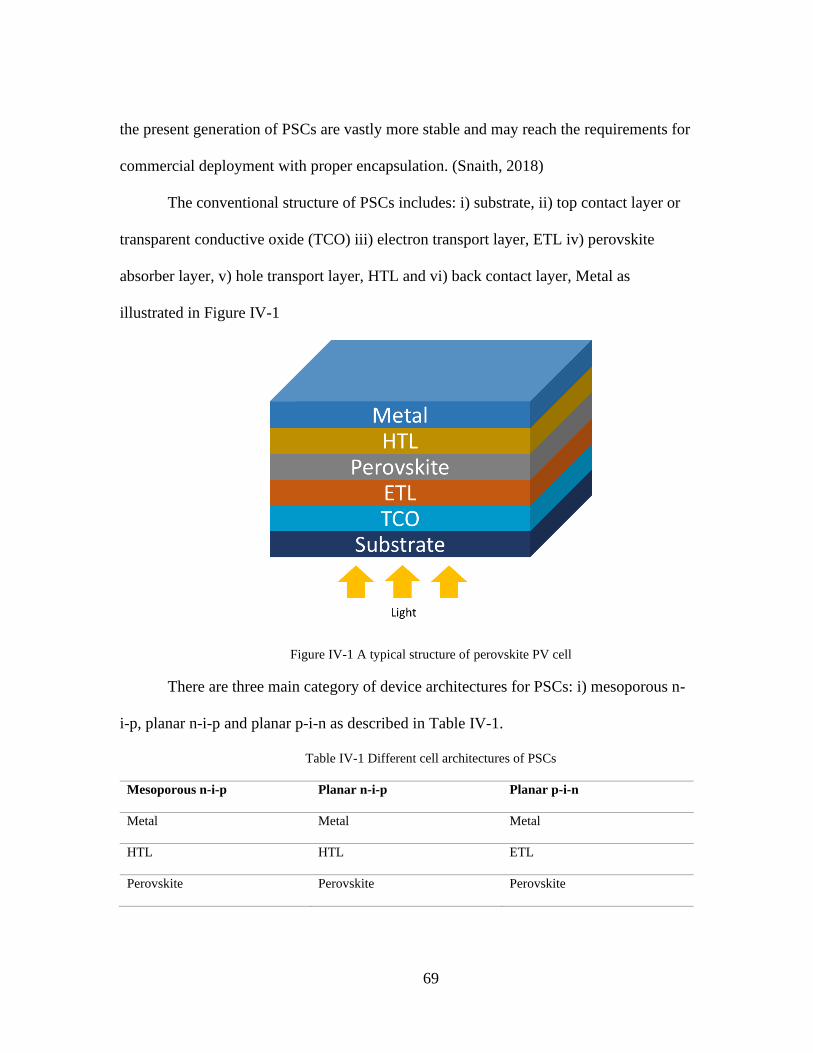
69

the present generation of PSCs are vastly more stable and may reach the requirements for

commercial deployment with proper encapsulation. (Snaith, 2018)

The conventional structure of PSCs includes: i) substrate, ii) top contact layer or

transparent conductive oxide (TCO) iii) electron transport layer, ETL iv) perovskite

absorber layer, v) hole transport layer, HTL and vi) back contact layer, Metal as

illustrated in Figure IV-1

Figure IV-1 A typical structure of perovskite PV cell

There are three main category of device architectures for PSCs: i) mesoporous n-

i-p, planar n-i-p and planar p-i-n as described in Table IV-1.

Table IV-1 Different cell architectures of PSCs

Mesoporous n-i-p Planar n-i-p Planar p-i-n

Metal Metal Metal

HTL HTL ETL

Perovskite Perovskite Perovskite

70

Mesoporous-ETL ETL HTL

TCO TCO TCO

Substrate Substrate Substrate

The mesoporous n-i-p structure was the first device architecture to be developed

based on dye-sensitized solar cells and has evolved significantly from the beginning of

PSC research (Li et al., 2018; Snaith, 2018). The mesoporous PSC device consists of a

nano porous ETL scaffold. The perovskite solution penetrates the scaffold and creates an

intermixed layer. The HTL and TCO are then sequentially deposited on the perovskite

layer to complete the cell structure. On the other hand, in planar architecture, a few

hundred nanometer thick compact perovskite film is sandwiched between ETL and HTL.

The simplicity of planar PSCs would suggest more potential for future industrial scale

configuration. However, at present, the mesoporous device architecture with a certified

PCE of 22% hold significant lead over the planar device architecture of which highest

certified configuration is 15% (Li et al., 2018; Snaith, 2018). With recent progress, the

HTL can be eliminated by using carbon or gold electrodes for certain n-i-p device

architecture. The planar p-i-n architecture is generally considered as inverted structure

compared to n-i-p structure (Li et al., 2018).

Typically, thin film PV modules (e.g. CdTe, CIGS) are fabricated by first

depositing the thin-film materials on single substrate and separating individual cells by

laser or mechanical scribing process. Perovskite module can be fabricated using similar

method (Li et al., 2018). Depending on the layout, interconnections occupy

approximately 3-10% of the module area which is inactive for power generation and a

71

significant source of power loss. The ratio of photoactive area and the total area is

defined as geometric fill factor (GFF) of the module and module with higher GFF can

generate more power for a given module size (Li et al., 2018). The GFF is highly

dependent on the configuration of the module and corresponding fabrication methods and

affects largely the performance of PV module. How to increase the GFF will play an

essential roll while up-scaling module fabrication towards commercial scale production

(Rong et al., 2018).

The National Renewable Energy Laboratory (NREL) released the “Champion

Photovoltaic Module Efficiency Chart” in March of 2019 devoting specifically to the

development of solar modules. In the NREL chart, the module sizes are divided into 4

categories:

• Mini or submodule: 200-800 cm2

• Small module: 800-6500 cm2

• Standard module: 6500 14000cm2

• Large module: 14000 cm2

Although, fabrication of perovskite module from 703 cm2 to 802 cm2 with PCE of

11.6% has been achieved, several issues are needed to be overcome for commercial scale

production of larger PSC module (Qiu et al., 2019).

The quality of the perovskite layer is of critical importance to obtain high

efficiency regardless of device architecture (N. Park, 2015). Until now, the most efficient

PSCs were fabricated using spin coating deposition method (Rong et al., 2018). However,

the material utilization efficiency of spin coating is extremely low as around 90%

72

material is lost during the process (Celik et al., 2016). In spin coating, thinning and

smoothing of the wet-solution films depends on the continuous centrifugal force which is

difficult to replicate in industrial scale deposition. Thus, the spin coating method cannot

be easily considered for scale up deposition (Li et al., 2018). Current research efforts

have been directed to develop scalable deposition methods for industrial scale fabrication

of PSC module. Different previous studies discussed different deposition method based

on both solution-based and vapor-based scalable techniques and analyzed the feasibility

of those techniques (Li et al., 2018; Qiu et al., 2019; Rong et al., 2018; Ye, Hong, Zhang,

& Liu, 2016). Scalable solution deposition methods for PSCs include, but not limited to,

blade coating, slot-die coating, spray coating, screen printing, meniscus coating, inkjet

printing and electrodeposition. Fabrication of solar module based on vapor deposition

methods such as physical vapor deposition (PVD), chemical vapor deposition (CVD),

hybrid CVD (HCVD) could also be promising. For more details about different

depositing method we refer (Yulia Galagan, 2018; Li et al., 2018; Qiu et al., 2019; Rong

et al., 2018).

In addition to scale up, efficiency and cost issues, the potential environmental

impacts of future PSC devices also gained interests in research communities. The impacts

due to energy consumption in manufacturing process and use of rare and toxic materials

may cause unintended environmental impacts. Therefore, a thorough environmental

evaluation is utmost necessity to identify environmental hotspots and guide further

development of perovskite PV technologies. We applied LCA-ET framework to compare

73

potential environmental performances of two emerging manufacturing processes of

perovskite PV module.

A number of LCA studies has been performed to evaluate the environmental

performances of different PSC configurations, raw materials and deposition methods

(Alberola-Borràs, Baker, et al., 2018; Alberola-Borràs, Vidal, Juárez-Pérez, et al., 2018;

Alberola-Borràs, Vidal, & Mora-Seró, 2018; Celik et al., 2017, 2016; García-Valverde,

Cherni, & Urbina, 2010; Gong et al., 2015; Uličná et al., 2018; Zhang, Gao, Deng, Zha,

& Yuan, 2017a; Zhang, Gao, Deng, Li, & Yuan, 2015; Zhang, Gao, Deng, Zha, & Yuan,

2017b) to support decision making towards commercialization of PSCs. Espinosa and

colleagues first utilized LCA to compare environmental impacts of two deposition

methods: spin coating and evaporation (Espinosa, Serrano-luján, Urbina, & Krebs, 2015).

Several other LCA studies performed LCA on lab scale process to provide

recommendations for further development (Alberola-Borràs, Vidal, Juárez-Pérez, et al.,

2018; Celik et al., 2016; Gong et al., 2015; Serrano-Lujan et al., 2015). LCA has been

also utilized to optimize composition of perovskite layer (Alberola-Borràs, Vidal, Juárez-

Pérez, et al., 2018; Alberola-Borràs, Vidal, & Mora-Seró, 2018). Some studies also

developed concepts of potential scalable device architecture and deposition methods and

perform LCA to evaluate potential environmental performances (Alberola-Borràs, Baker,

et al., 2018; Celik et al., 2016). Only a few LCA studies considered tandem

configurations, however we have not considered tandem configuration in this work.

There was also research effort to harmonize LCA studies to compare the findings from

different LCA studies of PSCs (Maranghi, Parisi, Basosi, & Sinicropi, 2019).

74

In this work, we demonstrate the application of the LCA-ET framework to

compare environmental performances of two novel potential large-scale manufacturing

processes of perovskite PV module (PSM): spray coating and screen printing. The LCA-

ET framework is utilized to provide information to compare between alternative

processes and to evaluate future environmental aspects of a potential scalable perovskite

module.

4.2 Perovskite case study: Goal, Scope and Scenario definition

The goal of this case study is to evaluate and compare future environmental

impacts of two potential scalable solution-processed perovskite solar modules by

applying LCA-ET framework. We have selected the following two manufacturing

processes for this case study:

4.2.1 Manufacturing process 1: Spray coating

Spray deposition is a low-cost, roll-to-roll compatible technique and this process

could potentially replace spin coating to produce perovskite with high power conversion

efficiency. Spray-coating is low-cost atmospheric deposition technique with high material

utilization and viable technique from a manufacturing perspective (Uličná et al., 2018)

We have selected spray-coating fabrication method for perovskite PV manufacturing

conducted by Uličná et al. (2018) as one of the fabrication processes to evaluate in this

study.

Uličná et al. (2018) demonstrated application of chlorine (Cl)-containing

methylamine lead iodide (MAPbI3) ink for spray-coating PSCs in ambient conditions.

FTO glass substrates is used as top contact layer. SnO2 is then spin coated for ETL

75

followed by deposition of perovskite layer via spray-coating method. Spiro-OMeTAD is

spin-coated as HTL and MoOx and Al are thermally evaporated as back contact layer to

complete the devices.

4.2.2 Manufacturing Process 2: Screen printing

Hu et al. (2017) fabricated a stable (10 X 10 cm2) printable mesoscopic perovskite

module which can be a potential fabrication process for stable large-scale perovskite

module production. We have selected this device architecture and manufacturing process

as fabrication process 2. FTO glass substrate is used as top contact layer. A patterned

TiO2 compact layer is deposited via spray deposition as blocking layer. A nanocrystalline

mesoporous TiO2 is screen printed followed by mesoporous ZrO2 layer and a

graphite/carbon layer. The mesoporous films are filled with perovskite solution. All

fabrication steps are performed in ambient temperature.

The summary of device architecture and fabrication method is included in Table

IV-2 and the detail inventory data is described in Appendix A.

76

Table IV-2 Comparison of fabrication material and deposition methods between spray coating and screen printing scenario.

Manufacturing Process Spray coating Screen printing

Device architecture and (deposition method)

Material structure FTO/SnO2/CH3NH3PbI3/S-OMeTAD/MoOx-

Al

FTO/TiO2/m-TiO2 + m-ZrO2+m-C/(5-AVA)x(MA)1-

xPbI3

Top contact layer FTO glass

(Screen printing)

FTO Glass with compact TiO2 as blocking layer

(Screen printing, Spray pyrolysis)

Electron transport layer SnO2

(Spin coating)

Mesoporous TiO2 scaffold

(Screen printing)

Perovskite absorber layer CH3NH3PbI3

(Spray coating)

(5-AVA)x(MA)1-xPbI3

(Screen printing)

Hole transport layer S-OMeTAD

(Spin coating)

Mesoporous ZrO2

(Screen printing)

Back contact layer MoOx-Al

(Thermal Evaporation)

Mesoporous carbon/graphite

(Screen printing)

Performance parameters

Module Power conversion efficiency

(PCE)

17.3% 10.4%

77

Performance ratio 75% 75%

Active area 70% 49%

78

According to NREL chart, the size of the standard module is between 6500 – 14000 cm2.

We defined the functional unit of this LCA study as fabrication of 1 m2 of the perovskite solar

module which is in the size range of standard module. All inventory data are generated by

aligning with this functional unit. However, while comparing environmental impacts with

existing commercial PV technologies, 1 kWh electricity generated for the entire life cycle is

considered as functional unit as the power conversion efficiency and active area varies

significantly between perovskite devices manufactured by different fabrication method.

This case study is a cradle to grave LCA study. We exclude module transportation from

the system boundary; this assumption was also used in previous studies (Celik et al., 2016; Gong

et al., 2015). We consider landfill as end-of-life disposal method in this study. When the modules

are landfilled, the lead is released to environment through leaching effect. The impact of lead

leaching from landfill area is only considered as impact from final disposal. No recycle of

material is considered in this study. Serrano-Lujan et al. (2015) considered up to 70% of lead

will be leached from the cells to the soil during first year in their study. We have considered

100% of lead will be leached from the module to the soil to account maximum environmental

impact in this case study. The balance of the system is not included in the system boundary so

that the LCA results can be compared with other PV technologies. Figure IV-2 represents the

general system boundary for all scenarios.

79

Figure IV-2 A general system boundary all scenarios of PSM manufacturing

PSCs are not commercially available technologies. Currently, the maximum reported

sizes of the perovskite modules are between 703 cm2 to 802 cm2 (Qiu et al., 2019) In this study,

the description of first fabrication process is obtained from Uličná et al. (2018) which describes

lab-scale fabrication process. Hu et al. (2017) reported fabrication of 10 by 10 cm2 perovskite

module and reported local outdoor stability of 1 month. They have also fabricated a 7 m2

perovskite solar panel utilizing screen printing. This fabrication method provides promising

prospect for large-scale production; however, further research and improvements are required for

industrial scale production. We can consider, perovskite PV module is between TRL 5-6. Thus,

the LCA results should be scaled-up to evaluate potential environmental impacts at industrial

scale.

In order to evaluate the potential environmental impacts at future industrial scale and to

allow comparison with existing commercial PV technologies, the LCA data should be scaled up.

We consider the following scenarios in this study.

Scenario 1: Spray coating

The fabrication process mentioned in Uličná et al. (2018) is considered as Scenario 1

without considering any scale-up assumptions.

80

Scenario 2: Screen printing

The fabrication process mentioned in Hu et al. (2017) is considered as Scenario 2 without

considering any scale-up assumptions.

Scenario 3: Modified spray coating

Modified spray deposition scenario is developed based on Scenario 1 utilizing scale-up

procedure of LCA-ET framework.

Scenario 4: Modified screen printing

Modified screen-printing scenario is developed based on Scenario 2 considering scale-up

assumption to allow comparison with commercial scale alternatives.

The detail of scale-up method is described section 3.2.2

4.3 Life cycle inventory and impact assessment

4.3.1 Data

Life cycle inventory data

We have utilized primary data (from description of lab scale fabrication methods) for

foreground modeling. If material utilized in the process is not given directly, the material

consumption is calculated using area and thickness of the substrate and density of the material

and material efficiency of the process. The lab scale data are linearly modified to calculate

inventory and impact assessment based on functional unit of 1 m2. In case of missing data, proxy

data of similar process from literature is used. Scale-up assumptions are made to perform LCA of

future industrial-scale process. For background data (e.g. inventory data for raw material

productions, solvent, component production, energy mix), we have utilized ecoinvent 3.5

database. If the data is not available in ecoinvent 3.5 database, we have created model in

openLCA software using synthesis process from literature to obtain characteristic data for impact

81

assessment. It is assumed that all PV module scenario use encapsulation to prevent module

degradation. The encapsulation data is obtained from previous LCA studies (Espinosa et al.,

2015; Gong et al., 2015). The performance ratio is considered as 75% recommended for roof-top

utility installation by methodology guidelines on LCA of PV electricity (Fthenakis et al., 2011).

The value of insolation is selected as (1.70 X 103 kW h m-2 per year) as typically selected in

assessment of PV technologies. Energy consumption data are obtained from fabrication

description of model or similar process from literature. The energy mix data used is US

electricity mix. The detail description of life cycle inventory of each scenario is given in

Appendix A.

Life cycle impact assessment

Tool for Reduction and Assessment of Chemicals and Other Environmental Impacts

(TRACI) is the most common impact assessment method in U.S. We have selected 10 TRACI

categories: i) acidification (kg SO2 eq), ii) ecotoxicity (CTUe), iii) eutrophication (kg N eq), iv)

global warming (kg CO2 eq), v) human health-carcinogenics, vi) human health-non-

carcinogenics, vii) ozone depletion (kg CFC-11 eq), viii) photochemical ozone formation (kg O3

eq), ix) resource depletion – fossil fuels and x) respiratory effects (kg PM 2.5 eq) for impact

assessment. We have used cumulative energy demand (CED) impact assessment method to

obtain primary energy demand associated with perovskite PV module. We sum up the energy

demand entries in CED impact assessment method i.e. fossil fuels, nuclear energy, solar energy,

wind energy, geothermal energy, and biomass to calculate primary energy demand. We have also

evaluated energy payback time (EPBT) for each scenario.

82

4.3.2 Scale-up

Step 1: LCA of lab-scale process

We performed the LCA of Scenario 1 and Scenario 2 in step 1. The primary data is

obtained from description of lab-scale procedure. This LCA results is utilized for relevance

analysis and to set-up scale-up strategy. Figure IV-3 and Figure IV-4 represent the LCA results

of Scenario 1 and Scenario 2 respectively.

From Figure IV-3, for spray coating manufacturing process, perovskite layer is the major

contributor to the potential environmental impacts in all impact categories: 94% in ADP, 82% in

HHC, 66% in ECO, 80% in EU, 94% in fossil fuel depletion, 88% in GWP, 66% in HHNC, 97%

in ODP, 79% in RE, 90% in smog formation, and 90% in CED. Back contact layer contributes in

ecotoxicity and respiratory effects. Lead emission from landfill contributes contribute 28% in

non-carcinogenic human health impact category, 5% in ecotoxicity and only 1% in carcinogenic

health impact. However, the health impact from lead leaching is significantly less compared to

the impact of perovskite absorber layer fabrication. The deposition of perovskite layer is the

main contributor to the environmental impacts which aligned with findings from literature.

(Celik et al., 2016)

Figure IV-4 represents relative contribution of environmental burdens from different

layer of screen-printing fabrication process. Similar to spray deposition process, the major

contributor is the perovskite layer except ecotoxicity. The top contact layer contributes 52% in

ecotoxicity while perovskite layer contributes 37%. In human health-noncarcinogenic category

perovskite layer contributes 38% while the contributions of top contact layer and lead emission

from landfill are 38% and 23%, respectively.

83

Figure IV-3 Relative contribution of different layers of perovskite PV module using spray coating

fabrication process. Data are normalized to represent percent contribution of each contributor. ADP: acidification

potential, ECO: ecotoxicity, EU: eutrophication, GWP: global warming potential, HHC: human health-

carcinogenic, HHNC: human health-non-carcinogenic, ODP: ozone depletion potential, PHOTO: photochemical

ozone formation, RD-FOSSIL: resource depletion-fossil fuels, RE: respiratory effects, CED: cumulative energy

demand.

Figure IV-4 Relative contribution of different layers of perovskite PV module using screen printing. Data

are normalized to represent percent contribution of each contributor.

0%10%20%30%40%50%60%70%80%90%

100%

Spray coating

Final disposal

Encapsulation

Cathode/back contact

HTL

Perovskite

ETL

TCO

0%

10%

20%

30%

40%

50%

60%

70%

80%

90%

100%

Screen printing

Final disposal

Encapsulation

Cathode/back contact

HTL

Perovskite

ETL

TCO

84

Step 2: Relevance analysis

From lab-scale LCA results, it is visible that, the perovskite absorber layer is the main

contributor in almost all impact categories for both fabrication process. We exclude the impact

from encapsulation layer for further analysis since the relative impact is not significant and we

assume that encapsulation process will not change due to scale-up procedure.

Step 3: Develop potential industrial-scale process

To develop future large-scale process, we replace relevant lab-scale equipment or process

by equipment or process suitable for large-scale manufacturing. At lab-scale, spin coating is the

most widely used deposition process for efficient PSCs. However, approximately 90% material

is lost during this process and thus we consider this unsuitable for large scale production (Celik,

Song, Cimaroli, Yan, Heben, et al., 2016). So, the spin coating process used for ETL and HTL in

spray-coating lab-scale manufacturing process are replaced by spray deposition method. In the

HTL layer, spiro-OMeTAD is used in the lab-scale process. However, this material is very

expensive, and its instability may represent potential challenge in the large-scale production. So,

to select potential industrial scale process, CuSCN is selected as HTL which shows high energy

conversion efficiency (15.6%) as inorganic HTL.(Celik, Song, Cimaroli, Yan, Heben, et al.,

2016) We consider this modified fabrication method as “Scenario 3: Modified spray coating”

For screen printing, the only change is the top contact layer deposition method. FTO

sputtering and laser substrate etching method is used for TCO layer deposition for reduced

material utilization. We define this modified fabrication method as “Scenario 3: Modified screen

printing”.

Step 4: Scale-up of each process step and linkage of process steps for synergy effects

85

The modified spray coating and modified screen printing consider changes in material

and energy consumption efficiency due to upscaling the process. The potential module power

conversion efficiency for modified screen printing is considered as 15% aligned with other LCA

study (Celik, Song, Cimaroli, Yan, Heben, et al., 2016) However, the module power conversion

efficiency for modified spray coating process remain same as lab scale process (17.3%) . The

active area is considered as 90% for this commercial scale production. The detail inventory data

for all scenarios are given in Appendix A.

Step 5: Perform LCA of defined scenarios and provide feedback

In this step, LCA of Scenario 3 and Scenario 4 is performed which consider scale-up

assumption. The LCA results can be used to guide further development of the perovskite module.

4.4 Life cycle results and discussions

We compare the life cycle impact assessment results between all four scenarios in Figure

IV-5. We normalized the data using the maximum impact value in each environmental category.

The increase of active area, use of carbon cathode, increase in energy efficiency, reduction of

solvent use are the key reasons for the lower environmental impacts. Based on the LCA results,

modified-screen printing module has better potential environmental performance i.e. the least

environmental impacts among four scenarios at future industrial scale. For all scenarios,

perovskite absorber layer is the main contributor of environmental burden. Modified spray

coating scenario reduces potential environmental impacts compared to spray coating considering

improved active area at large scale. However, compared to screen printing scenarios, the

environmental burdens are higher, even compared to screen printing scenario which doesn’t

consider scale-up assumptions.

86

Figure IV-5 also represents the relative contribution of different layer of PSM

manufactured by modified spray coating fabrication process. The perovskite layer is the major

contributor to the potential environmental impacts in all impact categories. However, there is

minor decrease in relative impacts compared to spray coating fabrication process. This is due to

the change of raw materials for HTL deposition that causes minor increase in relative

environmental impacts of HTL

For screen printing fabrication process, there is significant change in relative

environmental impacts of different layer of perovskite module. The perovskite layer is still the

major contributor of environmental impacts in all impact categories except acidification and

smog. However, the relative contribution decreases compared to screen printing process. This is

due to increase in relative environmental impacts of TCO and back contact layer.

87

Figure IV-5 Comparison of environmental impacts between different scenarios. Data are

normalized based on maximum environmental impact in each impact assessment category. ADP:

acidification potential, ECO: ecotoxicity, EU: eutrophication, GWP: global warming potential, HHC:

human health- carcinogenic, HHNC: human health-non-carcinogenic, ODP: ozone depletion potential,

PHOTO: photochemical ozone formation, RD-FOSSIL: resource depletion-fossil fuels, RE: respiratory

effects, CED: cumulative energy demand

Calculation of Energy Pay Back Time (EPBT)

We have calculated EPBT of the two scaled-up PSM scenarios using the following

equation (Celik, Song, Cimaroli, Yan, Heben, et al., 2016):

𝐸𝑃𝐵𝑇 = 𝑃𝐸𝐷 × 𝜀

𝐼 × 𝜇 × 𝑃𝑅 × 𝐶𝐹

Where,

EPBT= energy payback time (years)

PED = primary energy demand (MJprimary/m2)

ε = electrical to primary energy conversion factor (%), 35 %,

PR = performance ratio (%)

88

µ = efficiency (%)

I = insolation constant (kWh/m2-yr)

CF = conversion factor, 3.6 MJ/kWh

Figure IV-6 Comparison of EPBT between two scaled-up scenarios. The error bars represent 95%

confident region.

4.5 Uncertainty analysis

For prospective LCA of emerging technologies such as perovskite PV modules,

the LCA results depends on the data quality of input parameters. So, we assume that the

reliable results of the EPBT and environmental impacts can vary based on the uncertainty

involved with input variables. At early TRLs, several parameters such as power

conversion efficiencies, insolation, and lifetime, can exhibit inherent uncertainties. In this

case study, we have applied probability distributions to insolation and lifetime

0.00

1.00

2.00

3.00

4.00

5.00

6.00

Modified spray coating Modified screen printing

EPB

T (y

ears

)

89

parameters. We have used normal distribution for insolation and triangular distribution

for lifetime inputs. We have used 10000 Monte Carlo analysis using @Risk software tool

for uncertainty analysis. The summary of uncertain parameters considered in the study is

give in Table IV-3.

Table IV-3 Summary of uncertain parameters

Parameter Distribution Mean Standard deviation

Insolation (kW h m-2

per year)

Normal 1700 170

Lifetime (year) Triangular Min 1, Most likely 2, Max 5

The probability distributions for modified-screen printing perovskite module is

given in Figure IV-7 for EPBT Both distributions demonstrate range of results with

highest probabilities.

Figure IV-7 Probability distribution for modified screen printing perovskite module for EPBT

(YEARS)

0.1911 0.28432.5% 2.5%95.0%

0

2

4

6

8

10

12

14

16

18

0.1

5

0.2

0

0.2

5

0.3

0

0.3

5

0.4

0

EPBT (years)

EPBT (years)

90

Conclusion

The goal of this case study was to demonstrate the application on LCA-ET

framework for prospective evaluation of emerging perovskite solar module. We have

applied LCA-ET framework to compare among four perovskite module scenarios.

Among the four scenarios the modified-screen printing scenario shows superior

performance in terms of EPBT and minimizing environmental impacts. Considering

scaled up data, the potential environmental impact reduces for modified spray coating

scenario, however the environmental aspect is still lower compared to lab-scale of screen-

printing scenario. The perovskite absorber layer is the main contributor for environmental

impacts of PSMs. This finding also aligns with finding from previous literature (Celik,

Song, Cimaroli, Yan, Heben, et al., 2016). Further research should focus on reducing

environmental impacts of perovskite absorber layer.

.

91

CHAPTER FIVE

V. APPLICATION OF LCA-ET FRAMEWORK: A CASE STUDY OF ANAEROBIC

MEMBRANE BIOREACTORS FOR WASTEWATER TREATMENT

There is a growing interest in anaerobic treatment of domestic wastewater due to

the potential advantages of the anaerobic processes compared with aerobic alternatives.

No energy requirement for aeration, low biosolids production and conversion of organic

wastes into methane-rich biogas have made anaerobic processes a potential technology to

reduce wastewater treatment cost. However, a much longer solids retention time (SRT) is

required to gain enough microbial activity to meet the target organic removals. By

combining physical membrane separation with anaerobic biological processes, anaerobic

membrane bioreactors (AnMBR) has the potential to achieve required longer SRT and to

be a more sustainable wastewater treatment compared to aerobic alternatives. However,

the applications of AnMBR for domestic wastewater treatment are mostly at pilot-scale.

In this case study, we apply LCA-ET framework to evaluate and compare potential

environmental impacts of different AnMBR systems for treatment of domestic

wastewater under ambient conditions.

5.1 Introduction

Wastewater treatment plants (WWTPs) account for approximately 3% of the

electrical energy load in the United States, resulting about 45 million tons of greenhouse

gas annually (McCarty, Bae, & Kim, 2011). Due to population growth and more stringent

environmental requirements, the demand for electricity for WWTPs is expected to rise

92

significantly. Increasing energy cost and associated climate change concerns along with

worldwide shortage of energy, food and water have highlighted the demand for

sustainable wastewater treatment process. Domestic wastewater is now being considered

as a resource than as a waste, since wastewater can be a source of water, energy and

nutrients such as nitrogen (N) and phosphorus (P) for plants (McCarty et al., 2011).

Treated wastewater is now widely used for irrigation and domestic purposes to

reduce water consumption and utilize its nutrient contents (McCarty et al., 2011)

Similarly, domestic wastewater has also been used as an energy source, particularly

through anaerobic conversion of wastewater’s organic contents into useful methane

(CH4) gas. However, conventional methods of aerobic wastewater treatment combined

with anaerobic sludge digestion captures only a portion of the potential energy content of

wastewater. Moreover, aerobic treatment processes require aeration to oxidize organic

contents in the wastewater, which have high energy demand. Aerobic treatment processes

also generate large amount of sludge, which is also a growing concern due to high energy

consumption for treatment and disposal (P. J. Evans et al., 2019; Shin & Bae, 2017).

Anaerobic membrane bioreactor (AnMBR) systems are gaining interest as a

promising technology to treat domestic wastewater and recover energy in the form of

biogas (McCarty et al., 2011; Smith et al., 2014). AnMBR processes do not require

energy for aeration and can generate energy by converting organic wastes into methane-

rich biogas. AnMBR can generate a high-quality effluent while operating at reasonable

hydraulic retention times (HRT < 8 h) and generate far less sludge compared to aerobic

93

treatment processes (Cookney et al., 2016; McCarty et al., 2011; Shin & Bae, 2017;

Smith et al., 2014).

5.2 Configuration of AnMBRs

AnMBR is the integration of anaerobic biological process with physical

membrane separation process. There are different configurations of AnMBR system

based on location of membranes and methods to maintain membrane flux (P. J. Evans et

al., 2019; P. Evans, Vila, & Mccarty, 2018; Shin & Bae, 2017). Typically, the AnMBR

system consists of a primary anaerobic bioreactor and a secondary membrane bioreactor.

The primary bioreactor contains microorganisms that convert organic contents in

wastewater into methane reached biogas and carbon dioxide. The biogas from bioreactor

can be used to generate electricity, heat or transport fuel. The membrane can be in either

primary bioreactor or in secondary bioreactor. The secondary membrane bioreactor

contains ultrafiltration (UF) membrane which filter microorganisms and other suspended

solids from treated effluent (permeate). The purpose of the membrane is twofold: 1) to

produce a suspended solids-free permeate and 2) to maintain a high mixed liquor of

volatile suspended solids (VSS). Hollow fiber type membrane is used mostly, however

flat sheet type of membrane can also be applied (Shin & Bae, 2017). Similarly,

ultrafiltration membranes are generally used, however, use of microfiltration membrane

is also reported in literature (Shin & Bae, 2017).

Although AnMBR has several advantages compared to aerobic treatment

processes, issues such as membrane fouling and dissolved methane recovery hampered

widespread use of AnMBR process (Maaz et al., 2019; Smith et al., 2014). Fouling

94

control requires significant energy demand and operation cost while dissolved methane in

effluent represents loss of energy source and release of greenhouse gas (Smith et al.,

2014).

The AnMBR process can be different based on fouling control methods and type

of membrane used in the reactor. Three types of membrane scouring methods has been

used in pilot-scale systems: biogas sparging (GS), particle sparging (PS) and rotating

membrane (RM) (Shin & Bae, 2017). Hollow fiber and flat sheet are two membrane

types that are typically used. Figure V-1 presents schematic diagram of three membrane

scouring methods used in AnMBR.

Figure V-1 Schematic diagram of three types of AnMBRs: biogas sparging, particle sparging and

rotating membrane [adapted from Shin and Bae (2017)]

The most common membrane fouling control method in AnMBRs is biogas

sparging (Shin & Bae, 2017). In biogas sparging systems, uprising gas bubbles

95

introduced at the downside of membrane module to create turbulence in the liquid which

increases back transport of foulants from the membrane surface and thus scours

membrane. The intensity of biogas sparging is generally expressed as specific gas

demand per unit membrane demand area (SGDm) or superficial gas velocity in the

membrane tank. Sludge recirculation velocity is one of the important parameters to

control fouling in side stream AnMBRs (Lin et al., 2013; Shin & Bae, 2017).

In particle sparging AnMBR granular activated carbons (GAC) not only serve as

the support media for microorganism, but also act as a media for scouring membrane

surface. Particle sparging AnMBR is reported as less energy intensive compared to gas-

sparging AnMBRs. The rotating membrane AnMBR is another fouling control method

that used the rotation of membrane module with an axial rotation motor to create

turbulence. Though this method was suggested several decades ago, it has recently gained

attraction as an energy efficient fouling control method (Shin & Bae, 2017).

In this study, we apply LCA-ET framework to compare the potential environmental

impacts of gas-sparging AnMBR and GAC particle-sparging AnMBR to treat domestic

wastewater.

5.3 System boundary and functional unit

We consider medium domestic wastewater strengths (430 mg/L chemical oxygen

demand (COD)) and two wastewater temperatures (15 and 30 degrees C) in this study.

Typical composition of untreated domestic wastewater is used as influent water

composition. Sludge after thickening-dewatering and stabilization process sent to Landfill

for final disposal. We consider an average value of 100 km as distance between

96

wastewater treatment facilities and landfill area. Any environmental impact due to release

from sludge in landfill is not considered in the system boundary. Smith et al. (2014)

showed that construction phase environmental impacts are negligible compared to life

cycle impacts in their LCA study (Smith et al., 2014). The environmental impacts from

construction of wastewater facility is not considered in this LCA study. The operation or

use phase impacts are only included.

The functional unit of this LCA study is treatment of 5 million gallons per day

(MGD, 18,950 m3d-1) of domestic wastewater to achieve minimum U.S. EPA secondary

treatment effluent standards. Combustion of biogas in combined heat and power (CHP) is

considered as energy recovery process. Since, influent flow rates greater than 5 MGD are

required to produce biogas via anerobic digestion to be economically feasible for CHP,

treatment capacity is selected as 5 MGD per day.

In this case study, we have considered 4 AnMBR process scenarios. Scenarios 1

and 2 represents gas-sparged AnMBR configuration including vacuum operated hollow-

fiber gas-liquid contactor for dissolved methane removal operating at 30o C and 15o C,

respectively for treatment of medium strength wastewater treatment (abbreviated as

GS_30 and GS_15). Scenarios 3 and 4 represents GAC-fluidized AnMBR demonstration

configuration including similar hollow-fiber gas-liquid contactor for dissolved methane

removal (abbreviated as GAC_30 and GAC_15) operating a 30o C and 15o C,

respectively. Figure V-2 and Figure V-3 represents the system boundary of each scenario.

97

Figure V-2 Process configuration of Gas Sparged AnMBR

Figure V-3 Process configuration of GAC fluidized AnMBR

5.4 Life cycle inventory data

The membrane properties used for AnMBR are based on hollow fiber membrane.

The inventory information for membrane material is obtained from literature (P. J. Evans

et al., 2019; P. Evans et al., 2018; Smith et al., 2014). AnMBR methane production is

calculated assuming 350 L of methane is produced per kilogram of COD removed at

standard temperature and pressure. The value was adjusted for the different wastewater

temperatures. Presence of sulfate in wastewater reduces the amount of COD available for

methane conversion. Reduction of sulfate is considered when calculating methane

98

production. The dissolved methane concentration is in AnMBR effluent was calculated

using Henry’s Law assuming 1.5 times oversaturation following practice in other studies

(Smith et al., 2014). The recovery of dissolved methane is assumed to be 90 percent. Rest

dissolved methane in effluent is assumed to eventually release to the atmosphere. The

nutrients (nitrogen and phosphorus) recovery is not considered in this LCA study.

The AnMBR performance was based on results obtained from published literature

on lab and pilot scale studies (Shin & Bae, 2017; Smith et al., 2014). AnMBR COD

removal was assumed to be 90% at 30o C and 85% at 15o C for medium strength

domestic wastewater (Smith et al., 2014).

We assume waste activated sludge is thickened using a gravity belt-filter press.

Polymer and lime are added with the activated sludge and we assume sludge will be

disposed in landfill. For all raw material collection and sludge disposal to landfill,

transport impact is considered.

For the energy calculation, data obtained from the pilot-scale operation creates

best-case and worst-case scenarios (Shin & Bae, 2017). A combined heat and power

(CHP) unit is considered to calculate energy obtained from methane obtained from biogas

and dissolved methane recovery. The electricity and heat obtained from CHP unit are

considered as avoided burden. The grit removal and disinfection data are obtained from

literature (P. Evans et al., 2018) and are assumed equal for all AnMBR scenarios. Detail

inventory data are given in Appendix B. For background data (e.g. inventory data for raw

material productions, solvent, component production, energy mix), we have utilized

ecoinvent 3.5 database.

99

5.5 Life cycle impact assessment

Tool for Reduction and Assessment of Chemicals and Other Environmental

Impacts (TRACI) is the most common impact assessment method in U.S. We have

selected 10 TRACI categories: i) acidification (kg SO2 eq), ii) ecotoxicity (CTUe), iii)

eutrophication (kg N eq), iv) global warming (kg CO2 eq), v) human health-

carcinogenics, vi) human health-non-carcinogenics, vii) ozone depletion (kg CFC-11 eq),

viii) photochemical ozone formation (kg O3 eq), ix) resource depletion – fossil fuels and

x) respiratory effects (kg PM 2.5 eq) for impact assessment.

5.6 LCA results and discussion

Figure V-4 represents the comparison of potential environmental impacts between

all scenarios. Data are internally normalized based on maximum values in each impact

category. Gas-sparged AnMBRs have significantly more environmental impact compared

GAC particle-sparged AnMBRs. The difference in energy consumption is the main

reason behind this difference in environmental burden. Gas-sparged AnMBR at 15 degree

C (GS_15) has the highest environmental impacts in all impact categories. The energy

required for membrane bioreactor is the main contributor. Also due to lower temperature,

there is more dissolved methane in effluent and thus increases energy requirement to

recover the methane. GWP also increases due to increase in methane release into

environment.

The both GAC based AnMBRs shows better environmental impacts in all impact

categories. The average value energy consumption in bioreactor system is utilized for

GAC-fluidized AnMBR scenarios. The energy data range from 0.04 – 0.13 kWh/m3,

100

which is far below compared to energy consumption of gas sparged bioreactors that

ranges from 0.1- 0.65 kWh/m3. The lower energy consumption value is the reason for

these lower environmental impacts. Among all scenarios, only GAC_30 scenario shows

potential of net energy positive wastewater treatment process.

101

Figure V-4 Comparison of environmental impacts between all scenarios. ADP: acidification

potential, ECO: ecotoxicity, EU: eutrophication, GWP: global warming potential, HHC: human health-

carcinogenic, HHNC: human health-non-carcinogenic, ODP: ozone depletion potential, PHOTO:

photochemical ozone formation, RD-FOSSIL: resource depletion-fossil fuels, RE: respiratory effects, CED:

cumulative energy demand

-20%

0%

20%

40%

60%

80%

100%

Comparison of potential environmental impacts between scenarios

GS_30

GS_15

GAC_30

GAC_15

102

Figure V-5 Comparison between all scenarios including relative contribution of unit processes.

ADP: acidification potential, ECO: ecotoxicity, EU: eutrophication, GWP: global warming potential, HHC:

human health- carcinogenic, HHNC: human health-non-carcinogenic, ODP: ozone depletion potential,

PHOTO: photochemical ozone formation, RD-FOSSIL: resource depletion-fossil fuels, RE: respiratory

effects, CED: cumulative energy demand

103

Figure V-5 represents relative comparison of environmental impacts between different

scenarios including relative contribution of different process units. Apart from energy

consumption in bioreactor, the dissolved methane release are the major contributors. The

methane collected from bioreactor and dissolved methane are considered as avoided

burden and that reflects the negative GWP potential.

5.7 Conclusion

In this case study, we applied LCA-ET framework to compare environmental

impacts of gas sparging and particle sparging AnMBR bioreactors. The application of

LCA-ET framework can provide information to identify environmental hotspots and

enable to make change in process parameters at low technology level. It is also to be

noted that, extra care should be taken to address uncertainty associated with available

data and process model. Scenario analysis is utilized here to explore different bioreactor

configurations and effluent conditions (e.g. temperature). Other configurations (such as

rotary membrane bioreactor) or different process conditions can be used to develop new

scenarios and potential environmental impacts can be analyzed using LCA-ET

framework.

.

104

CHAPTER SIX

VI. CONCLUSIONS AND FUTURE WORK

In this study, we discussed the major methodological issues to perform LCA of

emerging technologies. We developed an ex-ante LCA framework including LCA scale-

up method to evaluate emerging technologies at low technology readiness level. We

demonstrated the application of LCA-ET framework using two emerging technologies as

case studies.

There are several research areas that should be explored further to extend the

utility of LCA to evaluate emerging technologies. In order to provide multiple

perspectives in the impact assessment and facilitate exploring trade-offs between

different impacts, several efforts have been taken to couple LCA with a multi-criteria

decision analytic approach (MCDA) (Linkov & Seager, 2011; Seager & Linkov, 2008;

Tsang, Bates, Madison, & Linkov, 2014; Zanghelini, Cherubini, & Soares, 2018). MCDA

refers to a group of methods used to expand understanding of a complex or uncertain

decision-making process such as assessing best options among emerging technologies

(e.g. nanomaterials). Integration of LCA and risk analysis (RA) is also proposed for

proactive assessment of emerging technologies to utilize advantage of the strengths of

each method (Linkov et al., 2017). RA quantifies potential exposure and hazard

associated with a specific material in a specific release scenario. Linkov et al. (2017)

argued that, because of contrast between two methods (e.g. differences between

boundaries, purpose, emphases), methodological integration is only possible at later

105

stages of analysis with complete datasets. They proposed that integration of results (not

methods) from LCA and RA in the context of MCDA is more promising approach to

provide better guidance to decision makers. Integration of diffusion of innovation

modeling techniques with LCA is also proposed which can assist to estimate the extent of

market penetration, displacement of existing technologies and rate of adoption and thus

allow the LCA community to develop future scenarios (Sharp & Miller, 2016).

Integration of additional tools with LCA should be explored further. However, more

discussion on this context is beyond the scope of this review. Another important area for

further research is to characterize life cycle impacts of novel environmental problems

created by emerging technologies (e.g. nanomaterials) that we have not discussed in this

contribution. Additional recommendations for future work are listed below:

• Sincere efforts should be undertaken to develop a data repository of life cycle

inventory data for various emerging materials, processes, and technologies so that

the data can be utilized for LCA of other similar technology concepts. This data

should include uncertainty distributions, technology or manufacturing readiness

level and other specific features such as data collection methods, assumptions,

and information regarding temporal and spatial variation.

• Results from LCA studies exploring scale up effects on life cycle inventory data

(e.g. scaling factors derived from empirical scaling relationship, change in LCA

data as technology development progress) should be placed in the public domain

wherever possible to aid future LCA studies of emerging technologies to handle

scale up issues.

106

• LCA results and associated uncertainties should be translated into language that

policy or decision makers can clearly understand and realize the proper

implications. A simple but robust standard reporting methods should be

developed to reduce inconsistencies in LCA results.

• LCA can be integrated with TEA tool for simultaneous evaluation of

economic and environmental performances of emerging technologies. Integrated

TEA-LCA tools help to reduce inconsistency between functional units, system

boundaries and assumptions considered while performing TEA and LCA

independently.

.

107

APPENDICES

108

Appendix A

A. Supporting information: LCA of perovskite solar PV module

Table A-1 Material and energy inventory of manufacturing of 1 kg PbI2 (Gong et al., 2015)

Process input Value Unit

Iodine (I2) 0.670 kg

Potassium hydroxide (KOH) 0.291 kg

Lead (Pb) 0.449 kg

Nitric acid (HNO3) 0.729 kg

Cumulative heat consumption 13.5 MJ

Cumulative Electricity

consumption

0.133 kWh

Process Outputs

Lead iodide (PbI2) 1.00 kg

Potassium nitrate (KNO3) 0.438 kg

Potassium iodate (KIO3) 0.135 kg

Nitric oxide (NO) 0.0434 kg

Waste 0.160 kg

Table A-2 Material and energy inventory of manufacturing of 1 kg CH3NH3I (Gong et al., 2015)


Hydrogen sulfide (H2S) 0.139 kg

Iodine (I2) 1.04 kg

Methylamine (CH3NH2) 0.581 kg

Ethanol (C2H6O) 7.31 kg

Diethyl ether (C4H10O) 20.8 kg

109

Cumulative heat consumption 8.30 MJ

Cumulative electricity

consumption

9.24 kWh

Process outputs kg

Methylammonium iodide

(CH3NH3I)

1.00 kg

Sulfur (S) 0.118 kg

Waste 29.9 kg

Table A-3 Material and energy inventory of manufacturing of 1 kg spiro-OMeTAD (Gong et al.,

2015)


Phenol (C6H6O) 0.724 kg

Sodium hydroxide (NaOH) 1.63 kg

Dimethyl sulfate (C2H6O4S) 0.485 kg

Potassium iodide (KI) 0.837 kg

Potassium iodate (KIO3) 0.412 kg

Methanol (CH4O) 2.47 kg

Hydrogen chloride (HCl) 5.04 kg

Hydrogen (H2) 0.0295 kg

Sodium methoxide (CH3ONa) 0.279 kg

Chlorobenzene (C6H5Cl) 0.966 kg

Nitric acid (HNO3) 1.08 kg

Sulfuric acid (H2SO4) 1.62 kg

110

Bromine (Br2) 0.604 kg

Coal tar 0.295 kg

Ethylene glycol (C2H6O) 1.06 kg

Aniline (C6H5NH2) 0.944 kg

Sodium nitrite (NaNO2) 0.221 kg

Sulfur dioxide (SO2) 0.407 kg

Magnesium (Mg) 0.0267 kg

Cumulative heat consumption 272 MJ

Cumulative electricity consumption 24.3 kWh

Process outputs kg

Spiro-OMeTAD (C81H88N4O8) 1.00 kg

Hydrogen bromide (HBr) 0.567 kg

2-Chloronitrobenzene (C6H4ClNO2) 0.428 kg

Waste 81.9 kg

Table A-4 Material and energy inventory of manufacturing of 1 kg FTO glass (Gong et al., 2015)


Silica sand 7.88E-01 kg

Soda ash 2.86E-01 kg

Limestone 1.41E-01 kg

Dolomite 9.10E-02 kg

Alumina 4.30E-02 kg

Cullet 1.10E-02 kg

Tin 5.01E-03 kg

111

Chloride 5.99E-03 kg

Heat consumption 7.88E-01 MJ

Air emissions

Carbon dioxide 1.28E-01 kg

Nitrogen oxide 3.00E-03 kg

Sulphur oxide 2.30E-03 kg

Methane 8.15E-04 kg

Particulates 1.00E-04 kg

Hydrogen fluoride 2.65E-05 kg

Lead 2.22E-05 kg

Arsenic 5.00E-06 kg

Nickel 5.56E-07 kg

Water emission

Chloride 8.20E-02 kg

COD 2.31E-04 kg

Sulfate 1.80E-04 kg

Suspended Solids 5.33E-05 kg

Fluoride 4.44E-05 kg

Mineral oil 3.56E-05 kg

Ammonia 1.78E-05 kg

Boric acid 7.11E-06 kg

Barium 5.33E-06 kg

Phenol 1.78E-06 kg

Chromium, Copper, tin, lead,

nickel, zinc

8.89E-07 kg

Arsenic, antimony 5.33E-07 kg

112

Cadmium 5.00E-07 kg

Solid waste 6.82E-02 kg

Table A-5 Material and energy inventory of manufacturing of 1 kg BL-TiO2 ink (Gong et al.,

2015)

Process parameter Value Unit

Titanium tetrachloride (TiCl4) 4.81E-02 kg

Isopropanol (C3H8O) 6.08E-02 kg

Acetone (C3H6O) 2.94E-02 kg

Acetic anhydride (C4H6O3) 5.18E-02 kg

Ethanol (C2H6O) 9.08E-01 kg

Heat consumption 1.54E-03 MJ

Electricity consumption 7.04E-05 kWh

Table A-6 Material and energy inventory of manufacturing of 1 kg nc-TiO2 ink (Gong et al., 2015)


Titanium dioxide (TiO2) 0.153 kg

Terpineol (C10H18O) 0.847 kg

113

Table A-7 Material and energy inventory of manufacturing of 1 kg silver paste (Gong et al., 2015)


Silver solid 7.00E-01 kg

Nitric acid (HNO3) 2.02E+00 kg

Reducing agent (C7H14) 8.82E-01 kg

Butyl acetate (C6H12O2) 3.00E-01 kg

Emissions

Nitrogen dioxide (NO2) 2.99E-01 kg

Table A-8 Material and energy inventory of manufacturing of 1 ethyl cellulose (Alberola-Borràs et

al., 2018)


Cellulose fiber 356.735 g

Ethanol 101.359 g

Hydrochloric acid 80.202 g

Electricity 1.35E-6 kWh

Emissions to water

Hydrogen chloride 80.202 g

Water 39.603 g

Table A-9 Material and energy inventory of manufacturing of 1 kg α-terpineol (Alberola-Borràs et

al., 2018)


Deionized water 116.692 g

114

Dichloromethane 550.611 g

Hydrogen, liquid 25.935 g

Acetone, liquid 753.053 g

Acetylene 337.602 g

Electricity 0.420 kWh

Emissions to water


Water 116.692 g

Organic chlorine compounds 431.03 g

Table A-10 Material and energy inventory of manufacturing of 1 kg titanium di-isopropoxide

bis(acetylacetonate) (Alberola-Borràs et al., 2018)


Acetone 637.786 g

Titanium tetrachloride 520.724 g

Isopropanol 659.968 g

electricity 1.35E-6 kWh

Emission to water

2-Propanol 329.984 g

Methane 87.849 g


115

Table A-11 Material and energy inventory of manufacturing of 1 kg 5-ammonium valeric acid

iodide (Alberola-Borràs et al., 2018)


Formic acid 187.828 g

Butane-1, 4-diol 367.49 g

Ammonia, liquid 69.541 g

Hydrogen, liquid 4.083 g

Iodine 518.18 g


Emissions to water

Water 146.996 g

Table A-12 Material and energy inventory of manufacturing of 1 kg 2-(2-butoxyethoxy) ethyl

acetate (Alberola-Borràs et al., 2018)


Acetic acid 293.992 g

Diethylene glycol 519.528 g

1-butanol 362.874 g


Emissions to air

Oxygen 78.329 g

Hydrogen 9.791 g

Emissions to water

Water 88.12 g

116

Table A-13 Material and energy inventory of manufacturing of 1 kg nitrocellulose (Alberola-

Borràs et al., 2018)


Cellulose fiber 162.237 g

Nitric acid 378.302 g


Emissions to water

Water 243.183 g

Table A-14 Life cycle inventory of 1 m2 perovskite module: lab-scale scenario

Source Parameter Value Unit

TCO layer: substrate

patterning

Material and energy inputs

FTO GLASS 5.04E+00 kg/m2

Ethanol 2.58E-02 kg/m2

Hydrogen chloride solution 6.95E-03 kg/m2

Deionized water 3.27E-02 kg/m2

Silver paste 8.81E-03 kg/m2

Ultrasonic cleaning 1.74E+00 MJ/m2

Screen printing 3.85E-02 MJ/m2

Sintering 5.50E+00 MJ/m2

Emissions



117

Silver 6.17E-03 kg/m2

Butyl acetate 2.64E-03 kg/m2

TCO layer: blocking layer

deposition


Compact TiO2 1.83E-02 kg/m2



Spray pyrolysis 3.44E-03 MJ/m2

Emissions

Acetic anhydride 9.46E-04 kg/m2

Acetone 5.38E-04 kg/m2

Isopropanol 1.23E-02 kg/m2

Titanium tetrachloride 1.76E-04 kg/m2

Electron-transport layer

deposition


nc-TiO2 layer 4.94E-03 kg/m2



Emissions

Terpineol 4.18E-03 kg/m2

Perovskite layer deposition Material and energy inputs

PbI2 1.38E-03 kg/m2

Dimethylformamide (DMF) 2.83E-03 kg/m2

CH3NH3I (MAI) 1.43E-04 kg/m2


PbI2 spin coating 8.08E-01 MJ/m2


Emissions

118

PbI2 9.66E-04 kg/m2

Dimethylformamide (DMF) 2.83E-03 kg/m2

Hole-transport layer deposition Material and energy inputs

Spiro-OMeTAD 8.50E-04 kg/m2

Chlorobenzene 1.18E-02 kg/m2

spiro-OMeTAD spin coating 8.08E-01 MJ/m2

Emissions



Cathode/back contact layer

deposition


Au 1.65E-03 kg/m2

Cathode evaporation 1.19E+01 MJ/m2

Emission

Au 2.97E-04 kg/m2

Encapsulation Material and energy inputs

Adhesive 2.02E-02 kg/m2

PET 6.17E-02 kg/m2

Encapsulation 1.48E-02 MJ/m2

End of life Pb Emission 1.86E-04 kg/m2

Table A-15 Life cycle inventory of 1 m2 perovskite module: spray-coating scenario


TCO layer deposition Material and energy inputs



119







Emissions





Electron-transport layer deposition


SnO2 2.08E-04 kg/m2


Pretreatment 1.94E+01 MJ/m2

Spray deposition 7.70E+01 MJ/m2

Post treatment 4.54E+01 MJ/m2

Emissions

Waste heat 2.84E+01 MJ/m2

Tin (to industrial soil) 3.28E-05 kg/m2


MACl 1.29E-01 kg/m2

NMP (N-methyl -2- pyrrolidinone) 4.47E+00 kg/m2

MAI 1.60E+00 kg/m2

PbI2 4.95E+00 kg/m2

N,N - dimethylformamide (DMF) 3.67E+00 kg/m2

120




Emissions

Methyl ammonium 3.45E-01 kg/m2

Pb 6.14E-01 kg/m2

Methyl formamide 8.93E-01 kg/m2





spiro-OMeTAD spin coating 8.08E-01 MJ/m2

Emissions



Cathode deposition Material and energy inputs

Al 4.05E-04 kg/m2

MoOx 7.04E-04 kg/m2

Evaporation 3.46E+01 MJ/m2

Vacuum 1.32E+02 MJ/m2

Emission

Al 2.03E-04 kg/m2




PET 6.17E-02 kg/m2

121


End of life Pb Emission 1.61E+00 kg/m2

Table A-16 Life cycle inventory of 1 m2 perovskite module: modified spray-coating scenario


TCO layer Material and energy inputs Unit









Electron-transport layer deposition Material and energy inputs

SnO2 2.08E-04 kg/m2





Emissions


Tin (to industrial soil) 3.28E-05 kg/m2


MACl 1.29E-01 kg/m2

122

NMP (N-methyl -2- pyrrolidinone) 4.47E+00 kg/m2

MAI 1.60E+00 kg/m2

PbI2 4.95E+00 kg/m2

N,N - dimethylformamide (DMF) 3.67E+00 kg/m2




Emissions

Methyl ammonium 3.45E-01 kg/m2

Pb 6.14E-01 kg/m2

Methyl formamide 8.93E-01 kg/m2



CuSCN 2.40E-03 kg/m2


Chemical Rxn 5.56E-08 MJ/m2


Deposition 3.17E+01 MJ/m2

Post-treatment 1.13E+01 MJ/m2

Emissions

Copper 5.95E-04 kg/m2

HCl 2.97E-04 kg/m2


Cathode deposition Material and energy inputs

Al 4.05E-04 kg/m2

MoOx 7.04E-04 kg/m2

123

Evaporation 3.46E+01 MJ/m2

Vacuum 1.32E+02 MJ/m2

Emission

Al 2.03E-04 kg/m2




PET 6.17E-02 kg/m2


End of life Pb Emission 1.61E+00 kg/m2

Table A-17 Life cycle inventory of 1 m2 perovskite module: screen-printing scenario



patterning










Emission


124





deposition






Emissions





m-TiO2 layer deposition Material and energy inputs

m-TiO2 layer 5.64E-03 kg/m2


Ethylcellulose 2.82E-03 kg/m2

2-(2-butoxyethoxy) ethyl acetate 5.64E-03 kg/m2

Process


Sintered at 500 deg. C for 30 min 1.80E+00 MJ/m2


Emissions




125


CO2 2.81E-03 kg/m2

Water vapor 1.01E-03 kg/m2

m-ZrO2 layer deposition Material and energy inputs

m-ZrO2 1.51E-02 kg/m2



Screen Printing 3.85E-02 MJ/m2



Emissions

m-ZrO2 3.79E-03 kg/m2



CO2 3.79E-03 kg/m2


Carbon back contact layer

deposition


Carbon/graphite 2.71E-02 kg/m2


Nitrocellolose 4.53E-03 kg/m2



Emissions




126

CO2 3.02E-03 kg/m2


Nitrogen dioxide 1.58E-03 kg/m2


AVAI 7.00E-03 kg/m2

GBL 1.19E+00 kg/m2

MAI 1.59E-01 kg/m2

PbI2 4.61E-01 kg/m2

Perovskite infiltration

(Annealing at 50 deg C for 60

min)

8.69E+01 MJ/m2

Emission

GBL 1.19E+00 kg/m2



PET 6.17E-02 kg/m2



Table A-18 Life cycle inventory of 1 m2 perovskite module: modified screen-printing scenario



patterning



FTO Sputtering 2.41E-03 MJ/m2

Laser substrate etching 9.50E+00 MJ/m2

127


deposition






Emissions





m-TiO2 layer deposition Material and energy inputs







m-ZrO2 layer deposition Material and energy inputs

m-ZrO2 8.18E-03 kg/m2





Carbon back contact layer

deposition




128





AVAI 1.63E-04 kg/m2

GBL 2.75E-02 kg/m2

MAI 3.69E-03 kg/m2

PbI2 1.07E-02 kg/m2

Process

Perovskite infiltration (Annealing

at 50 deg C for 60 min)

8.69E+01 MJ/m2



PET 6.17E-02 kg/m2



129

Table A-19 Life cycle impact of 1 m2 perovskite module: lab-scale scenario

Impact category ADP HHC ECO EU RD-FOSSIL GWP HHNC ODP RE SMOG CED

Reference unit kg SO2 eq CTUh CTUe kg N eq MJ surplus kg CO2 eq CTUh kg CFC-11 eq kg PM2.5 eq kg O3 eq MJ

TCO 6.56E-02 1.45E-06 1.10E+03 1.06E-01 8.03E+00 7.53E+00 2.18E-05 8.44E-07 1.34E-02 1.19E+00 1.11E+02

ETL 2.14E-03 7.88E-08 2.01E+01 6.74E-03 8.30E-01 8.73E-01 2.91E-07 2.22E-07 2.43E-03 3.08E-02 1.60E+01

Perovskite 1.06E-03 3.08E-08 7.88E+00 2.61E-03 4.69E-01 3.66E-01 2.00E-07 3.70E-08 9.10E-04 1.39E-02 7.15E+00

HTL 6.79E-04 1.85E-08 4.72E+00 1.75E-03 2.94E-01 2.19E-01 7.30E-08 2.60E-08 5.23E-04 9.06E-03 4.38E+00

Cathode/back contact 2.97E-01 4.87E-05 3.32E+04 6.08E+00 3.48E+01 2.76E+01 1.38E-03 3.89E-06 4.27E-02 6.49E+00 4.35E+02

Encapsulation 1.37E-03 1.71E-08 2.31E+00 1.19E-03 8.38E-01 3.77E-01 8.27E-08 4.47E-08 2.98E-04 2.31E-02 8.12E+00

Final disposal 0.00E+00 3.76E-11 4.11E-02 0.00E+00 0.00E+00 0.00E+00 1.32E-08 0.00E+00 0.00E+00 0.00E+00 0.00E+00

Table A-20 Life cycle impact of 1 kWh electricity production from perovskite module: lab-scale scenario



TCO 4.04E-04 8.95E-09 6.77E+00 6.50E-04 4.94E-02 4.64E-02 1.34E-07 5.19E-09 8.28E-05 7.35E-03 6.84E-01

ETL 1.32E-05 4.85E-10 1.24E-01 4.15E-05 5.11E-03 5.38E-03 1.79E-09 1.36E-09 1.50E-05 1.89E-04 9.86E-02

Perovskite 6.53E-06 1.90E-10 4.85E-02 1.61E-05 2.89E-03 2.25E-03 1.23E-09 2.28E-10 5.60E-06 8.55E-05 4.40E-02

HTL 4.18E-06 1.14E-10 2.91E-02 1.08E-05 1.81E-03 1.35E-03 4.49E-10 1.60E-10 3.22E-06 5.58E-05 2.70E-02

Cathode/back contact 1.83E-03 3.00E-07 2.04E+02 3.74E-02 2.14E-01 1.70E-01 8.51E-06 2.39E-08 2.63E-04 4.00E-02 2.68E+00

Encapsulation 8.45E-06 1.05E-10 1.42E-02 7.35E-06 5.16E-03 2.32E-03 5.09E-10 2.75E-10 1.84E-06 1.42E-04 5.00E-02


130

Table A-21 Life cycle impact of 1 m2 perovskite module: spray-coating scenario



TCO 6.54E-02 1.45E-06 1.10E+03 1.05E-01 7.79E+00 7.48E+00 2.18E-05 8.41E-07 1.34E-02 1.19E+00 1.09E+02

ETL 4.76E-02 1.84E-06 4.78E+02 1.60E-01 1.87E+01 2.02E+01 6.84E-06 1.59E-06 5.75E-02 6.89E-01 3.72E+02

Perovskite 2.66E+00 2.70E-05 5.11E+03 1.89E+00 8.30E+02 3.96E+02 2.56E-04 1.22E-04 5.35E-01 2.42E+01 8.59E+03

HTL 6.79E-04 1.85E-08 4.72E+00 1.75E-03 2.94E-01 2.19E-01 7.30E-08 2.60E-08 5.23E-04 9.06E-03 4.38E+00

Cathode/back contact 5.67E-02 2.28E-06 6.42E+02 2.03E-01 2.20E+01 2.38E+01 1.13E-05 1.87E-06 6.82E-02 8.25E-01 4.38E+02


Final disposal 0.00E+00 1.05E-09 1.15E+00 0.00E+00 0.00E+00 0.00E+00 3.70E-07 0.00E+00 0.00E+00 0.00E+00 0.00E+00

Table A-22 Life cycle impact of 1 kWh electricity production from perovskite module: spray-coating scenario



TCO 2.12E-04 4.70E-09 3.56E+00 3.41E-04 2.52E-02 2.42E-02 7.07E-08 2.73E-09 4.35E-05 3.86E-03 3.54E-01

ETL 1.54E-04 5.95E-09 1.55E+00 5.18E-04 6.06E-02 6.56E-02 2.22E-08 5.14E-09 1.86E-04 2.23E-03 1.20E+00

Perovskite 8.63E-03 8.75E-08 1.66E+01 6.13E-03 2.69E+00 1.28E+00 8.29E-07 3.94E-07 1.73E-03 7.83E-02 2.78E+01

HTL 2.20E-06 5.98E-11 1.53E-02 5.67E-06 9.52E-04 7.09E-04 2.36E-10 8.43E-11 1.69E-06 2.94E-05 1.42E-02




131

Table A-23 Life cycle impact of 1 m2 perovskite module: modified spray-coating scenario



TCO 6.54E-02 1.45E-06 1.10E+03 1.05E-01 7.79E+00 7.48E+00 2.18E-05 8.41E-07 1.34E-02 1.19E+00 1.09E+02

ETL 4.76E-02 1.84E-06 4.78E+02 1.60E-01 1.87E+01 2.02E+01 6.84E-06 1.59E-06 5.75E-02 6.89E-01 3.72E+02

Perovskite 2.66E+00 2.70E-05 5.11E+03 1.89E+00 8.30E+02 3.96E+02 2.56E-04 1.22E-04 5.35E-01 2.42E+01 8.59E+03

HTL 3.66E-02 1.40E-06 3.82E+02 1.22E-01 1.43E+01 1.54E+01 5.40E-06 1.21E-06 4.38E-02 5.26E-01 2.83E+02




Table A-24 Life cycle impact of 1 kWh electricity production from perovskite module: modified spray-coating scenario



TCO 1.65E-04 3.66E-09 2.77E+00 2.66E-04 1.96E-02 1.89E-02 5.50E-08 2.12E-09 3.38E-05 3.00E-03 2.75E-01

ETL 1.20E-04 4.63E-09 1.21E+00 4.03E-04 4.72E-02 5.10E-02 1.72E-08 4.00E-09 1.45E-04 1.74E-03 9.37E-01

Perovskite 6.71E-03 6.81E-08 1.29E+01 4.77E-03 2.09E+00 9.97E-01 6.45E-07 3.06E-07 1.35E-03 6.09E-02 2.16E+01

HTL 9.23E-05 3.54E-09 9.63E-01 3.08E-04 3.60E-02 3.88E-02 1.36E-08 3.05E-09 1.10E-04 1.33E-03 7.13E-01




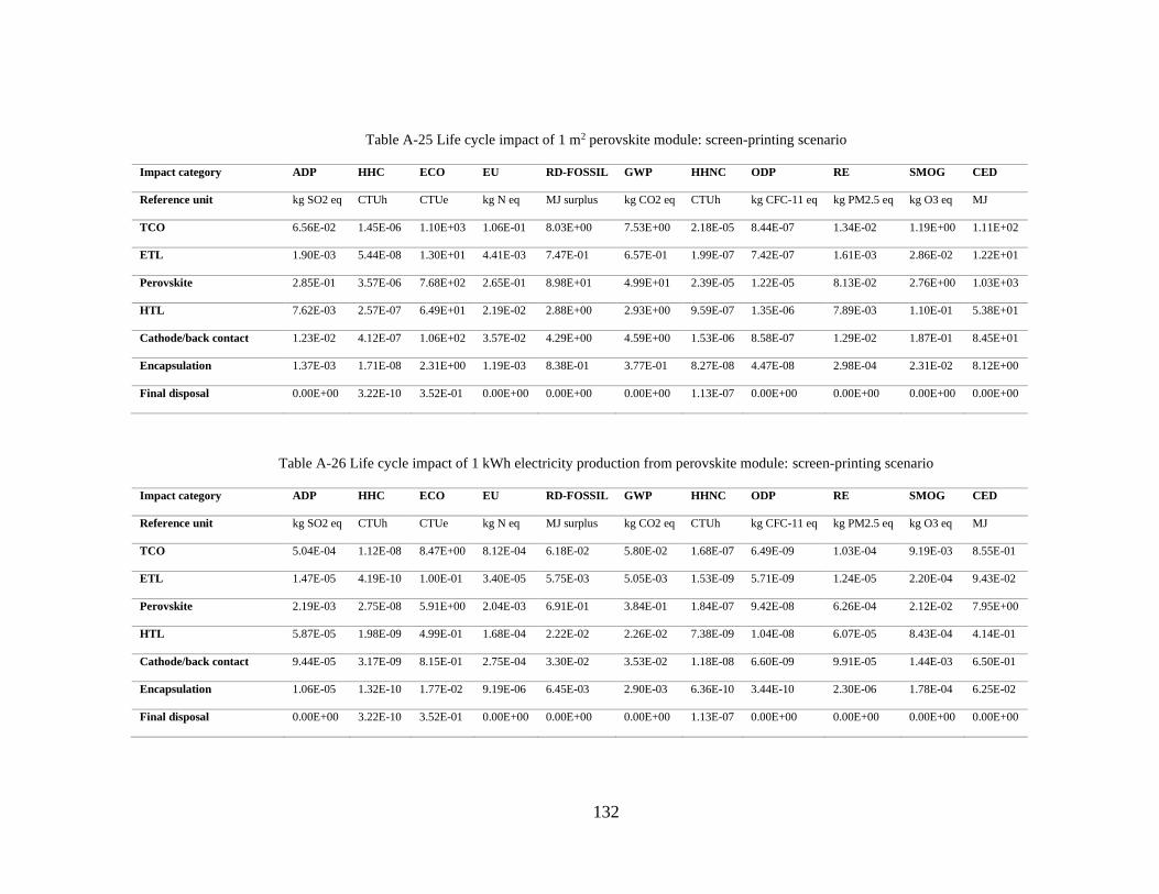
132

Table A-25 Life cycle impact of 1 m2 perovskite module: screen-printing scenario



TCO 6.56E-02 1.45E-06 1.10E+03 1.06E-01 8.03E+00 7.53E+00 2.18E-05 8.44E-07 1.34E-02 1.19E+00 1.11E+02

ETL 1.90E-03 5.44E-08 1.30E+01 4.41E-03 7.47E-01 6.57E-01 1.99E-07 7.42E-07 1.61E-03 2.86E-02 1.22E+01

Perovskite 2.85E-01 3.57E-06 7.68E+02 2.65E-01 8.98E+01 4.99E+01 2.39E-05 1.22E-05 8.13E-02 2.76E+00 1.03E+03

HTL 7.62E-03 2.57E-07 6.49E+01 2.19E-02 2.88E+00 2.93E+00 9.59E-07 1.35E-06 7.89E-03 1.10E-01 5.38E+01




Table A-26 Life cycle impact of 1 kWh electricity production from perovskite module: screen-printing scenario



TCO 5.04E-04 1.12E-08 8.47E+00 8.12E-04 6.18E-02 5.80E-02 1.68E-07 6.49E-09 1.03E-04 9.19E-03 8.55E-01

ETL 1.47E-05 4.19E-10 1.00E-01 3.40E-05 5.75E-03 5.05E-03 1.53E-09 5.71E-09 1.24E-05 2.20E-04 9.43E-02

Perovskite 2.19E-03 2.75E-08 5.91E+00 2.04E-03 6.91E-01 3.84E-01 1.84E-07 9.42E-08 6.26E-04 2.12E-02 7.95E+00

HTL 5.87E-05 1.98E-09 4.99E-01 1.68E-04 2.22E-02 2.26E-02 7.38E-09 1.04E-08 6.07E-05 8.43E-04 4.14E-01

Cathode/back contact 9.44E-05 3.17E-09 8.15E-01 2.75E-04 3.30E-02 3.53E-02 1.18E-08 6.60E-09 9.91E-05 1.44E-03 6.50E-01



133

Table A-27 Life cycle impact of 1 m2 perovskite module: modified screen-printing scenario



TCO 3.87E-02 7.65E-07 8.18E+01 2.96E-02 5.40E+00 5.32E+00 3.33E-06 4.58E-07 1.01E-02 6.90E-01 7.70E+01

ETL 1.15E-03 2.92E-08 6.70E+00 2.29E-03 4.51E-01 3.66E-01 1.06E-07 5.90E-07 8.45E-04 1.60E-02 6.89E+00

Perovskite 3.50E-02 1.18E-06 3.03E+02 1.02E-01 1.33E+01 1.33E+01 4.64E-06 1.23E-06 3.63E-02 4.76E-01 2.46E+02

HTL 3.86E-03 1.29E-07 3.25E+01 1.10E-02 1.46E+00 1.47E+00 4.81E-07 7.24E-07 3.95E-03 5.55E-02 2.71E+01




Table A-28 Life cycle impact of 1 kWh electricity production from perovskite module: modified screen-printing scenario



TCO 1.12E-04 2.22E-09 2.38E-01 8.59E-05 1.57E-02 1.55E-02 9.68E-09 1.33E-09 2.95E-05 2.00E-03 2.24E-01

ETL 3.35E-06 8.48E-11 1.95E-02 6.65E-06 1.31E-03 1.06E-03 3.07E-10 1.71E-09 2.45E-06 4.65E-05 2.00E-02

Perovskite 1.02E-04 3.43E-09 8.79E-01 2.95E-04 3.85E-02 3.85E-02 1.35E-08 3.58E-09 1.05E-04 1.38E-03 7.15E-01

HTL 1.12E-05 3.74E-10 9.43E-02 3.18E-05 4.23E-03 4.28E-03 1.40E-09 2.10E-09 1.15E-05 1.61E-04 7.86E-02

Cathode/back contact 3.24E-05 1.20E-09 3.08E-01 1.03E-04 1.25E-02 1.33E-02 4.45E-09 2.49E-09 3.74E-05 4.67E-04 2.45E-01



134

Appendix B

B. Supporting information: Case study of LCA of AnMBR for domestic wastewater

treatment

Table B-1 Typical composition of domestic wastewater influent

Contaminants Unit Medium strength

Solids, total (TS) mg/L 720

Dissolved, total (TDS) mg/L 500

Fixed mg/L 300

Volatile mg/L 200

Suspended solids, total (TSS) mg/L 210

Fixed mg/L 50

Volatile mg/L 160

Settleable solids mg/L 10

Biochemical oxygen demand, 5-d mg/L 190

Total organic carbon mg/L 140

Chemical oxygen demand (COD) mg/L 430

Nitrogen (Total as N) mg/L 40

Organic mg/L 15

Free ammonia mg/L 25

Nitrites mg/L 0

Nitrates mg/L 0

Phosphorus (total as P) mg/L 7

Organic mg/L 2

Inorganic mg/L 5

135

Chlorides mg/L 50

Sulfate mg/L 30

Table B-2 Life cycle inventory of GS_30 scenario

Source Value Unit

Primary treatment (screening and grit removal)

Screening and grit removal 630 kWh/day

Equalization 35 kWh/day

Waste produced 850 kg/day

Transport to Landfill 4.459 km/day

Secondary treatment (AnMBR_gas sparged)

Biological treatment energy consumption 7163.1 kWh/day

NaOCl (100%) 40 kg/day

H2O 226 kg/day

Transport 0.696 km/day

PVC (UF membrane) 19.9 kg/day


Polyester (UF membrane) 2.2 kg/day


Sludge management

Sludge Thickening and Dewatering-Biosolids energy consumption 143 kWh/day

Polyacrylamide 6.5188 kg/day

Hydrotreated Light Petroleum Distillates 6.5188 kg/day

H2O 6.5188 kg/day


136

Quicklime 110.8196 kg/day


Biosolids (for land fill) 651.88 kg/day

Transport 100 km/day

Biogas Handling, Treatment and Use

Biogas treatment and storage energy consumption 351 kWh/day

Bioreactor-Methane (energy co-products) 3238.681 kWh/day

Dissolved-Methane (energy co-products) 2147.757 kWh/day

Excess heat (energy co-product) 17064.24 MJ/day

CO2 (biogas + CHP unit) 2334.367 kg/day

Dissolved methane removal energy consumption 2471 kWh/day

PVC-Methane contactor 0.66 kg/day


Polypropylene-Methane contactor 0.17 kg/day


CH4 emission 66.15098 kg/day

Disinfection

NaOCL 341 kg/day

H2O 1932 kg/day

Transport 6 km/day

137

Table B-3 Life cycle inventory of GS_15 scenario

Source Value Unit






Secondary treatment (AnMBR_gas sparged)



H2O 226 kg/day






Sludge management

Sludge Thickening and Dewatering-of Biosolids energy consumption 143 kWh/day



H2O 6.5188 kg/day






138













Disinfection

NaOCL 341 kg/day

H2O 1932 kg/day

Transport 6 km/day

Table B-4 Life cycle inventory of GAC_30 scenario

Source Value Unit





Secondary treatment (AnMBR_GAC)


139


H2O 226 kg/day






GAC 109 kg/day

Transport 0.286 kg/day

Sludge management




H2O 6.5188 kg/day












Dissolved methane removal 2471 kWh/day

140






Disinfection

NaOCL 341 kg/day

H2O 1932 kg/day

Transport 6 km/day

Table B-5 Life cycle inventory of GAC_15 scenario

Source Value Unit






Secondary treatment (AnMBR_GAC)



H2O 226 kg/day




141



GAC 109 kg/day

Transport 0.286 kg/day

Sludge management




H2O 6.5188 kg/day


















142

Disinfection

NaOCL 341 kg/day

H2O 1932 kg/day

Transport 6 km/day

143

Table B-6 Life cycle impact of GS_30 scenario

Impact category ADP HHC ECO EU RD-FOSSIL GWP HHNC ODP RE SMOG

Reference unit kg SO2 eq CTUh CTUe kg N eq MJ surplus kg CO2 eq CTUh kg CFC-11 eq kg PM2.5 eq kg O3 eq

Primary treatment

Screen and grit removal 6.72E-01 2.51E-05 2.38E+03 2.36E+00 2.83E+02 3.04E+02 8.30E-05 2.36E-05 8.75E-01 1.03E+01

Equalization 3.73E-02 1.40E-06 1.32E+02 1.31E-01 1.57E+01 1.69E+01 4.61E-06 1.31E-06 4.86E-02 5.70E-01

Waste transport 5.22E-03 9.73E-08 1.37E+01 2.58E-03 4.44E+00 2.14E+00 5.64E-07 4.89E-07 1.06E-03 6.74E-02

Secondary treatment

NaOCl 5.34E-01 8.13E-06 1.15E+03 4.97E-01 8.48E+01 1.07E+02 4.60E-05 5.99E-05 1.60E-01 6.65E+00

PVC (UF membrane) 1.32E-01 2.73E-06 1.81E+02 2.89E-02 1.34E+02 4.27E+01 6.23E-06 7.40E-07 1.05E-02 2.43E+00

Polyester (UF membrane) 3.83E-02 4.45E-07 6.14E+01 3.55E-02 2.29E+01 1.10E+01 2.23E-06 1.42E-06 8.76E-03 6.93E-01

AnMBR_ENERGY 7.64E+00 2.86E-04 2.71E+04 2.68E+01 3.22E+03 3.46E+03 9.43E-04 2.69E-04 9.94E+00 1.17E+02

Sludge management

Polyacrylamide 1.24E-01 7.13E-07 9.78E+01 1.11E-01 1.11E+02 2.15E+01 3.93E-06 7.31E-06 1.40E-02 9.81E-01

Quicklime 1.79E-01 7.96E-07 1.15E+02 7.30E-02 9.39E+01 1.35E+02 4.89E-06 1.05E-05 2.75E-02 2.54E+00

Sludge_management_energy 1.53E-01 5.71E-06 5.41E+02 5.35E-01 6.42E+01 6.90E+01 1.88E-05 5.36E-06 1.99E-01 2.33E+00

Transport 8.98E-02 1.67E-06 2.35E+02 4.43E-02 7.64E+01 3.69E+01 9.71E-06 8.41E-06 1.82E-02 1.16E+00

Biogas management

Biogas Handling_energy 3.75E-01 1.40E-05 1.33E+03 1.31E+00 1.58E+02 1.69E+02 4.62E-05 1.32E-05 4.87E-01 5.72E+00

CO2 0.00E+00 0.00E+00 0.00E+00 0.00E+00 0.00E+00 2.33E+03 0.00E+00 0.00E+00 0.00E+00 0.00E+00

Bioreactor methane -3.46E+00 -1.29E-04 -1.23E+04 -1.21E+01 -1.46E+03 -1.56E+03 -4.27E-04 -1.21E-04 -4.50E+00 -5.28E+01

Dissolved methane -2.29E+00 -8.57E-05 -8.13E+03 -8.04E+00 -9.65E+02 -1.04E+03 -2.83E-04 -8.05E-05 -2.98E+00 -3.50E+01

144

Excess heat -8.25E-01 -4.66E-06 -4.36E+02 -1.20E-01 -1.62E+03 -6.15E+02 -1.69E-05 -6.67E-05 -5.67E-02 -1.39E+01

PVC-Methane contactor 4.39E-03 9.05E-08 6.01E+00 9.59E-04 4.44E+00 1.42E+00 2.06E-07 2.45E-08 3.47E-04 8.06E-02

PP-Methane contactor 1.14E-03 9.44E-09 6.01E-01 1.55E-04 1.74E+00 3.49E-01 7.96E-09 3.22E-09 9.11E-05 1.61E-02

CH4 emission 0.00E+00 0.00E+00 0.00E+00 0.00E+00 0.00E+00 1.65E+03 0.00E+00 0.00E+00 0.00E+00 0.00E+00

Dissolved Methane Removal_energy 2.64E+00 9.86E-05 9.35E+03 9.25E+00 1.11E+03 1.19E+03 3.25E-04 9.27E-05 3.43E+00 4.02E+01

Disinfection

Disinfection_NaOCL 4.56E+00 6.94E-05 9.78E+03 4.24E+00 7.25E+02 9.11E+02 3.92E-04 5.11E-04 1.36E+00 5.67E+01

Table B-7 Life cycle impact of GS_15 scenario



Primary treatment




Secondary treatment


Citric acid 0.00E+00 0.00E+00 0.00E+00 0.00E+00 0.00E+00 0.00E+00 0.00E+00 0.00E+00 0.00E+00 0.00E+00




Sludge management

145





Biogas management

Biogas Handling energy 3.75E-01 1.40E-05 1.33E+03 1.31E+00 1.58E+02 1.69E+02 4.62E-05 1.32E-05 4.87E-01 5.72E+00

CO2 0.00E+00 0.00E+00 0.00E+00 0.00E+00 0.00E+00 2.18E+03 0.00E+00 0.00E+00 0.00E+00 0.00E+00








Disinfection


Table B-8 Life cycle impact of GAC_30 scenario



Primary treatment


146



Secondary treatment





GAC 2.33E+00 2.00E-05 2.07E+03 1.33E+00 3.21E+02 4.16E+02 9.04E-05 2.69E-05 3.17E-01 2.29E+01

Sludge management





Biogas management

Biogas Hand_energy 3.75E-01 1.40E-05 1.33E+03 1.31E+00 1.58E+02 1.69E+02 4.62E-05 1.32E-05 4.87E-01 5.72E+00

CO2 0.00E+00 0.00E+00 0.00E+00 0.00E+00 0.00E+00 2.33E+03 0.00E+00 0.00E+00 0.00E+00 0.00E+00







147


Disinfection


Table B-9 Life cycle impact of GAC_15 scenario



Primary treatment




Secondary treatment





GAC 2.33E+00 2.00E-05 2.07E+03 1.33E+00 3.21E+02 4.16E+02 9.04E-05 2.69E-05 3.17E-01 2.29E+01

Sludge management





148

Biogas management

Biogas Hand_energy 3.75E-01 1.40E-05 1.33E+03 1.31E+00 1.58E+02 1.69E+02 4.62E-05 1.32E-05 4.87E-01 5.72E+00

CO2 0.00E+00 0.00E+00 0.00E+00 0.00E+00 0.00E+00 2.18E+03 0.00E+00 0.00E+00 0.00E+00 0.00E+00








Disinfection


149

REFERENCES

Alberola-Borràs, J. A., Baker, J. A., De Rossi, F., Vidal, R., Beynon, D., Hooper, K. E.

A., … Mora-Seró, I. (2018). Perovskite Photovoltaic Modules: Life Cycle

Assessment of Pre-industrial Production Process. IScience, 9, 542–551.

https://doi.org/10.1016/j.isci.2018.10.020

Arena, M., Azzone, G., & Conte, A. (2013). A streamlined LCA framework to support

early decision making in vehicle development. Journal of Cleaner Production, 41,

105–113. https://doi.org/10.1016/j.jclepro.2012.09.031

Arvidsson, R., Kushnir, D., Sanden, B. A., & Molander, S. (2014). Prospective life cycle

assessment of graphene production by ultrasonication and chemical reduction.

Environmental Science and Technology, 48(8), 4529–4536.

https://doi.org/10.1021/es405338k

Arvidsson, R., & Molander, S. (2017). Prospective Life Cycle Assessment of Epitaxial

Graphene Production at Different Manufacturing Scales and Maturity. Journal of

Industrial Ecology, 21(5), 1153–1164. https://doi.org/10.1111/jiec.12526

Arvidsson, R., Tillman, A.-M., Sandén, B. A., Janssen, M., Nordelöf, A., Kushnir, D., &

Molander, S. (2017). Environmental Assessment of Emerging Technologies:

Recommendations for Prospective LCA. Journal of Industrial Ecology, 00(0), 1–9.

https://doi.org/10.1111/jiec.12690

Azapagic, A., & Clift, R. (1999). The application of life cycle assessment to process

optimisation. Computers & Chemical Engineering, 23(10), 1509–1526.

https://doi.org/10.1016/S0098-1354(99)00308-7

150

Caduff, M., Huijbregts, M. A. J., Althaus, H., & Hendriks, A. J. (2011). Power-Law

Relationships for Estimating Mass, Fuel Consumption and Costs of Energy

Conversion Equipments. Environ. Sci. Technol, 45, 751–754.

https://doi.org/10.1021/es103095k

Caduff, M., Huijbregts, M. A. J., Althaus, H. J., Koehler, A., & Hellweg, S. (2012). Wind

power electricity: The bigger the turbine, the greener the electricity? Environmental

Science and Technology, 46(9), 4725–4733. https://doi.org/10.1021/es204108n

Caduff, M., Huijbregts, M. A. J., Koehler, A., Althaus, H. J., & Hellweg, S. (2014).

Scaling Relationships in Life Cycle Assessment: The Case of Heat Production from

Biomass and Heat Pumps. Journal of Industrial Ecology, 18(3), 393–406.


Celik, I., Mason, B. E., Phillips, A. B., Heben, M. J., & Apul, D. (2017). Environmental

Impacts from Photovoltaic Solar Cells Made with Single Walled Carbon Nanotubes.

Environmental Science and Technology, 51(8), 4722–4732.

https://doi.org/10.1021/acs.est.6b06272

Celik, I., Song, Z., Cimaroli, A. J., Yan, Y., & Heben, M. J. (2016). Solar Energy

Materials & Solar Cells Life Cycle Assessment ( LCA ) of perovskite PV cells

projected from lab to fab. Solar Energy Materials and Solar Cells, 156, 157–169.

https://doi.org/10.1016/j.solmat.2016.04.037

Celik, I., Song, Z., Cimaroli, A. J., Yan, Y., Heben, M. J., & Apul, D. (2016). Life Cycle

Assessment ( LCA ) of perovskite PV cells projected from lab to fab. Solar Energy

Materials and Solar Cells, 156, 157–169.

151

https://doi.org/10.1016/j.solmat.2016.04.037

Celik, I., Song, Z., Phillips, A. B., Heben, M. J., & Apul, D. (2018). Life cycle analysis of

metals in emerging photovoltaic (PV) technologies: A modeling approach to

estimate use phase leaching. Journal of Cleaner Production, 186, 632–639.

https://doi.org/10.1016/j.jclepro.2018.03.063

Cookney, J., Mcleod, A., Mathioudakis, V., Ncube, P., Soares, A., Jefferson, B., &

Mcadam, E. J. (2016). Dissolved methane recovery from anaerobic effluents using

hollow fibre membrane contactors. Journal of Membrane Science, 502, 141–150.

https://doi.org/10.1016/j.memsci.2015.12.037

Cooper, D. R., & Gutowski, T. G. (2018). Prospective Environmental Analyses of

Emerging Technology: A Critique, a Proposed Methodology, and a Case Study on

Incremental Sheet Forming. Journal of Industrial Ecology, 0(0), 1–14.


Cucurachi, S., Borgonovo, E., & Heijungs, R. (2016). A Protocol for the Global

Sensitivity Analysis of Impact Assessment Models in Life Cycle Assessment. Risk

Analysis, 36(2), 357–377. https://doi.org/10.1111/risa.12443

Cucurachi, Stefano, Giesen, C. Van Der, & Guinée, J. (2018). Ex-ante LCA of emerging

technologies. Procedia CIRP, 69(May), 463–468.

https://doi.org/10.1016/j.procir.2017.11.005

Curran, M. A. (2006). Life cycle assessment: principles and practice. Cincinnati, Ohio:

US Environmental Protection Agency, EPA/600/R-06/060.

DOD (U.S. Department of Defense). (2017). Manufacturing Readiness Level ( MRL )

152

Deskbook: Version 2017. Prepared by the OSD Manufacturing Technology

Program in collaboration with The Joint Service/Industry MRL Working Group.

Washington, DC.

DOE. (2014). Targeted Algal Biofuels and Bioproducts (TABB). Retrieved from

https://energy.gov/eere/bioenergy/bioenergy-technologies-office-closed-funding-

opportunities#Targeted Algal Biofuels and Bioproducts (TABB)

DOE. (2015). Quadrennial Technology review An assessment of energy technologies and

research Chapter 6 : Innovating Clean Energy Technologies in Advanced

Manufacturing.

DOE. (2016). DOE: MEGA-BIO: Bioproducts to Enable Biofuels. Retrieved from


opportunities#MEGA BIO Bioproducts to Enable Biofuels

DOE. (2017). Integrated Biorefinery Optimization. Retrieved from


opportunities#Integrated Biorefinery Optimization

DOE (U.S. Department of Energy). (2010). Standard Review Plan (SRP): Technology

Readiness Assessment Report. March 2008. Office of Environmental Management,

US DOE, Washington D.C.

Earles, J. M., & Halog, A. (2011). Consequential life cycle assessment: A review.

International Journal of Life Cycle Assessment, 16(5), 445–453.

https://doi.org/10.1007/s11367-011-0275-9

Evans, P. J., Parameswaran, P., Lim, K., Bae, J., Shin, C., Ho, J., & McCarty, P. L.

153

(2019). A comparative pilot-scale evaluation of gas-sparged and granular activated

carbon-fluidized anaerobic membrane bioreactors for domestic wastewater

treatment. Bioresource Technology, 288(November 2018), 120949.

https://doi.org/10.1016/j.biortech.2019.01.072

Evans, P., Vila, P., & Mccarty, P. (2018). Anaerobic Membrane Bioreactor ( AnMBR )

for Sustainable Wastewater Treatment.

Finkbeiner, M., Hoffmann, R., Ruhland, K., Liebhart, D., & Stark, B. (2006). Application

of Life Cycle Assessment for the Environmental Certificate of the Mercedes-Benz

S-Class, 11(4), 240–246.

Galagan, Y., Coenen, E. W. C., Verhees, W. J. H., & Andriessen, R. (2016). Towards the

scaling up of perovskite solar cells and modules. Journal of Materials Chemistry A,

4(15), 5700–5705. https://doi.org/10.1039/c6ta01134a

Galagan, Yulia. (2018). Perovskite Solar Cells: Toward Industrial-Scale Methods. The

Journal of Physical Chemistry Letters, 9, 4326–4335. review-article.

https://doi.org/10.1021/acs.jpclett.8b01356

Gavankar, S., Anderson, S., & Keller, A. A. (2015). Critical Components of Uncertainty

Communication in Life Cycle Assessments of Emerging Technologies:

Nanotechnology as a Case Study. Journal of Industrial Ecology, 19(3), 468–479.


Gavankar, S., Suh, S., & Keller, A. A. (2015). The Role of Scale and Technology

Maturity in Life Cycle Assessment of Emerging Technologies: A Case Study on

Carbon Nanotubes. Journal of Industrial Ecology, 19(1), 51–60.

154


Gong, J., Darling, S. B., & You, F. (2015). Perovskite photovoltaics: Life-cycle

assessment of energy and environmental impacts. Energy and Environmental

Science, 8(7), 1953–1968. https://doi.org/10.1039/c5ee00615e

Graedel, T.E., & Allenby, B. R. (2011). Industrial Ecology and Sustainable Engineering.

Graedel, Thomas E, Allenby, B. R., & Comrie, P. R. (1995). Matrix Approaches to

Abrigdged Life Cycle Assessment, 29(3), 134A-139A.

Graedel, Thomas E, & Saxton, E. (2002). Improving the Overall Environmental

Performance of Existing Telecommunications Facilities, 7(4), 219–224.

Green, M. A., Ho-Baillie, A., & Snaith, H. J. (2014). The emergence of perovskite solar

cells. Nature Photonics, 8(7), 506–514. https://doi.org/10.1038/nphoton.2014.134

Grubb, G. F., & Bakshi, B. R. (2011). Life Cycle of Titanium Dioxide Nanoparticle

Production. Journal of Industrial Ecology, 15(1), 81–95.

https://doi.org/10.1111/j.1530-9290.2010.00292.x

Guinée, J. B., Cucurachi, S., Henriksson, P. J. G., & Heijungs, R. (2018). Digesting the

alphabet soup of LCA Digesting the alphabet soup of LCA. The International

Journal of Life Cycle Assessment, (May), 6. https://doi.org/10.1007/s11367-018-

1478-0

Guinée, J., Gorrée, M., & Heijungs, R. (2002). Handbook on life cycle assessment.

Operational Guide to the ISO Standards. https://doi.org/10.1007/0-306-48055-7

Harris, T. M., Eranki, P. L., & Landis, A. E. (2019). Life cycle assessment of proposed

space elevator designs. Acta Astronautica, 161(July 2018), 465–474.

155

https://doi.org/10.1016/j.actaastro.2019.02.028

Hawkins, T. R., Singh, B., Majeau-Bettez, G., & Strømman, A. H. (2013). Comparative

Environmental Life Cycle Assessment of Conventional and Electric Vehicles.

Journal of Industrial Ecology, 17(1), 53–64. https://doi.org/10.1111/j.1530-

9290.2012.00532.x

Heijungs, R., & Huijbregts, M. A. J. (2004). A review of approaches to treat uncertainty

in LCA. In International Congress on Environmental Modeling and Software (p. 8).

https://doi.org/http://www.iemss.org/iemss2004/pdf/lca/heijarev.pdf

Hetherington, A. C., Borrion, A. L., Griffiths, O. G., & McManus, M. C. (2014). Use of

LCA as a development tool within early research: Challenges and issues across

different sectors. International Journal of Life Cycle Assessment, 19(1), 130–143.

https://doi.org/10.1007/s11367-013-0627-8

Hicks, B. J., Culley, S., Larsson, A., & Larsson, T. (2009). A methodology for evaluating

technology readiness during product development. In Proceedings of ICED 09, the

17th Internantional Conference on Engineering Design. Design Organization and

Management, Palo Alto, CA, USA.

Hicks, B., Larsson, A., Culley, S., & Larsson, T. (2009). A METHODOLOGY FOR

EVALUATING TECHNOLOGY REDINESS DURING PRODUCT

DEVELOPMENT. In INTERNATIONAL CONFERENCE ON ENGINEERING

DESIGN, ICED (pp. 157–168).

Hillman, K. M., & Sanden, B. A. (2008). Exploring technology paths: The development

of alternative transport fuels in Sweden 2007-2020. Technological Forecasting and

156

Social Change, 75(8), 1279–1302. https://doi.org/10.1016/j.techfore.2008.01.003

Hischier, R., Salieri, B., & Pini, M. (2017). Most important factors of variability and

uncertainty in an LCA study of nanomaterials – Findings from a case study with

nano titanium dioxide. NanoImpact, 7(May), 17–26.

https://doi.org/10.1016/j.impact.2017.05.001

Hospido, A., Davis, J., Berlin, J., & Sonesson, U. (2010). A review of methodological

issues affecting LCA of novel food products. International Journal Life Cycle

Assessment, 15, 44–52. https://doi.org/10.1007/s11367-009-0130-4

Hu, Y., Si, S., Mei, A., Rong, Y., Liu, H., Li, X., & Han, H. (2017). Stable Large-Area

(10 × 10 cm 2 ) Printable Mesoscopic Perovskite Module Exceeding 10%

Efficiency. Solar RRL, 1(2), 1600019. https://doi.org/10.1002/solr.201600019

Hung, C. R., Ellingsen, L. A. W., & Majeau-Bettez, G. (2018). LiSET: A Framework for

Early-Stage Life Cycle Screening of Emerging Technologies. Journal of Industrial

Ecology, 00(0), 1–12. https://doi.org/10.1111/jiec.12807

Hur, T., Lee, J., Ryu, J., & Kwon, E. (2005). Simplified LCA and matrix methods in

identifying the environmental aspects of a product system, 75, 229–237.

https://doi.org/10.1016/j.jenvman.2004.11.014

Igos, E., Benetto, E., Meyer, R., Baustert, P., & Othoniel, B. (2018). How to treat

uncertainties in life cycle assessment studies? International Journal of Life Cycle

Assessment, 1–14. https://doi.org/10.1007/s11367-018-1477-1

International Organisation for Standardization. (1998). Environmental management - life

cycle assessment - principles and framework. ISO, Geneva, Switzerland: ISO 14040.

157

ISO. (2006). Environmental management - Life Cycle Assessment - Principles and

Framework. International Organization for Standardization, 3, 20.

https://doi.org/10.1016/j.ecolind.2011.01.007

Jungbluth, N., Bauer, C., Dones, R., & Frischknecht, R. (2005). Life cycle assessment for

emerging technologies: Case studies for photovoltaic and wind power. International

Journal of Life Cycle Assessment, 10(1), 24–34.

https://doi.org/10.1065/lca2004.11.181.3

Khanna, V., Bakshi, B. R., & Lee, L. J. (2008). Carbon nanofiber production: Life cycle

energy consumption and environmental impact. Journal of Industrial Ecology,

12(3), 394–410. https://doi.org/10.1111/j.1530-9290.2008.00052.x

Kunnari, E., Valkama, J., Keskinen, M., & Mansikkama, P. (2009). Environmental

evaluation of new technology : printed electronics case study. Journal of Cleaner

Production, 17, 791–799. https://doi.org/10.1016/j.jclepro.2008.11.020

Kunnari, E., Valkama, J., Keskinen, M., & Mansikkamäki, P. (2009). Environmental

evaluation of new technology: printed electronics case study. Journal of Cleaner

Production, 17(9), 791–799. https://doi.org/10.1016/j.jclepro.2008.11.020

Kushnir, D., & Sanden, B. A. (2011). Multi-level energy analysis of emerging

technologies: A case study in new materials for lithium ion batteries. Journal of

Cleaner Production, 19(13), 1405–1416.


Lacirignola, M., Blanc, P., Girard, R., Pérez-López, P., & Blanc, I. (2016). LCA of

emerging technologies: addressing high uncertainty on inputs’ variability when

158

performing global sensitivity analysis. Science of The Total Environment, 578, 268–

280. https://doi.org/10.1016/j.scitotenv.2016.10.066

Li, Z., Klein, T. R., Kim, D. H., Yang, M., Berry, J. J., Van Hest, M. F. A. M., & Zhu, K.

(2018). Scalable fabrication of perovskite solar cells. Nature Reviews Materials,

3(4), 18017. https://doi.org/10.1038/natrevmats.2018.17

Lin, H., Peng, W., Zhang, M., Chen, J., Hong, H., & Zhang, Y. (2013). A review on

anaerobic membrane bioreactors: Applications, membrane fouling and future

perspectives. Desalination, 314, 169–188.

https://doi.org/10.1016/j.desal.2013.01.019

Linkov, I., & Seager, T. P. (2011). Coupling Multi-Criteria Decision Analysis, Life-

Cycle Assessment, and Risk Assessment for Emerging Threats. Environ. Sci.

Technol, 45(1), 5068–5074. https://doi.org/10.1021/es100959q

Linkov, I., Trump, B. D., Wender, B. A., Seager, T. P., Kennedy, A. J., & Keisler, J. M.

(2017). Integrate life-cycle assessment and risk analysis results, not methods. Nature

Nanotechnology, 12(8), 740–743. https://doi.org/10.1038/nnano.2017.152

Lloyd, S. M., & Ries, R. (2008). Characterizing, Propagating, and Analyzing Uncertainty

in Life-Cycle Assessment: A Survey of Quantitative Approaches. Journal of

Industrial Ecology, 11(1), 161–179. https://doi.org/10.1162/jiec.2007.1136

Maaz, M., Yasin, M., Aslam, M., Kumar, G., Atabani, A. E., Idrees, M., … Kim, J.

(2019). Anaerobic membrane bioreactors for wastewater treatment: Novel

configurations, fouling control and energy considerations. Bioresource Technology,

283(December 2018), 358–372. https://doi.org/10.1016/j.biortech.2019.03.061

159

Maranghi, S., Parisi, M. L., Basosi, R., & Sinicropi, A. (2020). LCA as a Support Tool

for the Evaluation of Industrial Scale-UP. In S. Maranghi & C. Brondi (Eds.), Life

Cycle Assessment in the Chemical Product Chain (pp. 125–141). Springer.

McCarty, P. L., Bae, J., & Kim, J. (2011). Domestic wastewater treatment as a net energy

producer-can this be achieved? Environmental Science and Technology, 45(17),

7100–7106. https://doi.org/10.1021/es2014264

McManus, M. C., Taylor, C. M., Mohr, A., Whittaker, C., Scown, C. D., Borrion, A. L.,

… Yin, Y. (2015). Challenge clusters facing LCA in environmental decision-

making—what we can learn from biofuels. International Journal of Life Cycle

Assessment, 20(10), 1399–1414. https://doi.org/10.1007/s11367-015-0930-7

Miller, S. A., & Keoleian, G. A. (2015). Framework for Analyzing Transformative

Technologies in Life Cycle Assessment. https://doi.org/10.1021/es505217a

Moni, S. M., Mahmud, R., High, K., & Carbajales-Dale, M. (2019). Life cycle

assessment of emerging technologies: A review. Journal of Industrial Ecology,

24(1), 52–63. https://doi.org/10.1111/jiec.12965

Nielsen, P. ., & Wenzel, H. (2002). Integration of environmental aspects in product

development: a stepwise procedure based on quantitative life cycle assessment.

Journal of Cleaner Production, 10(3), 247–257. https://doi.org/10.1016/S0959-

6526(01)00038-5

Park, N. G., Grätzel, M., Miyasaka, T., Zhu, K., & Emery, K. (2016). Towards stable and

commercially available perovskite solar cells. Nature Energy, 1(11).

https://doi.org/10.1038/nenergy.2016.152

160

Parvatker, A. G., Tunceroglu, H., Sherman, J. D., Coish, P., Anastas, P., Zimmerman, J.

B., & Eckelman, M. J. (2019). Cradle-to-Gate Greenhouse Gas Emissions for

Twenty Anesthetic Active Pharmaceutical Ingredients Based on Process Scale-Up

and Process Design Calculations. ACS Sustainable Chemistry & Engineering, 7,

6580–6591. research-article. https://doi.org/10.1021/acssuschemeng.8b05473

Pérez-lópez, P., Lacirignola, M., Girard, R., Blanc, P., & Blanc, I. (2017). Global

sensitivity analysis in LCA of emerging technologies : Accounting for inputs ’

variability. In SETAC Europe 2017 - 27th Annual Meeting (pp. 4–5). Brussels,

Belgium.

Pérez-lópez, P., Montazeri, M., Feijoo, G., Teresa, M., & Eckelman, M. J. (2018).

Science of the Total Environment Integrating uncertainties to the combined

environmental and economic assessment of algal biore fi neries : A Monte Carlo

approach. Science of the Total Environment, 626, 762–775.

https://doi.org/10.1016/j.scitotenv.2017.12.339

Piccinno, F., Hischier, R., Seeger, S., & Som, C. (2016). From laboratory to industrial

scale: a scale-up framework for chemical processes in life cycle assessment studies.

Journal of Cleaner Production, 135, 1085–1097.


Piccinno, F., Hischier, R., Seeger, S., & Som, C. (2018). Predicting the environmental

impact of a future nanocellulose production at industrial scale: Application of the

life cycle assessment scale-up framework. Journal of Cleaner Production, 174, 283–

295. https://doi.org/10.1016/j.jclepro.2017.10.226

161

Po, R., Bernardi, A., Calabrese, A., Carbonera, C., Corso, G., & Pellegrino, A. (2014).

From lab to fab: how must the polymer solar cell materials design change? – an

industrial perspective. Energy & Environmental Science, 7(3), 925.

https://doi.org/10.1039/c3ee43460e

Prado-Lopez, V., Seager, T. P., Chester, M., Laurin, L., Bernardo, M., & Tylock, S.

(2014). Stochastic multi-attribute analysis (SMAA) as an interpretation method for

comparative life-cycle assessment (LCA). International Journal of Life Cycle

Assessment, 19(2), 405–416. https://doi.org/10.1007/s11367-013-0641-x

Prado, V., & Heijungs, R. (2018). Implementation of stochastic multi attribute analysis

(SMAA) in comparative environmental assessments. Environmental Modelling and

Software, 109(August), 223–231. https://doi.org/10.1016/j.envsoft.2018.08.021

Prado, V., Wender, B. A., & Seager, T. P. (2017). Interpretation of comparative LCAs:

external normalization and a method of mutual differences. International Journal of

Life Cycle Assessment, 22(12), 2018–2029. https://doi.org/10.1007/s11367-017-

1281-3

Raluy, R. G., Serra, L., & Uche, J. (2005). LCA Case Studies Life Cycle Assessment of

Water Production Technologies Part 1 : Life Cycle Assessment of Different

Commercial Desalination Technologies ( MSF , MED , RO ), 10(4), 285–293.

Ravikumar, D., Seager, T. P., Cucurachi, S., Prado, V., & Mutel, C. (2018). Novel

Method of Sensitivity Analysis Improves the Prioritization of Research in

Anticipatory Life Cycle Assessment of Emerging Technologies. Environmental

Science and Technology, 52(11), 6534–6543. research-article.

162


Rong, Y., Ming, Y., Ji, W., Mei, A., Hu, Y., & Han, H. (2018). Toward Industrial-Scale

Production of Perovskite Solar Cells: Screen Printing, Slot-Die Coating, and

Emerging Techniques. The Journal of Physical Chemistry Letters, 9, 2707–2713.

https://doi.org/10.1021/acs.jpclett.8b00912

Sanden, B. A., Jonasson, K. M., Karlstrom, M., & Tillman, A. (2005). LCA of emerging

technologies: a methodological framework. In LCM2005 (pp. 5–8). Barcelona.

Schmidt, T. M., Larsen-Olsen, T. T., Carlé, J. E., Angmo, D., & Krebs, F. C. (2015).

Upscaling of Perovskite Solar Cells: Fully Ambient Roll Processing of Flexible

Perovskite Solar Cells with Printed Back Electrodes. Advanced Energy Materials,

5(15), 1–9. https://doi.org/10.1002/aenm.201500569

Seager, T. P., & Linkov, I. (2008). Coupling multicriteria decision analysis and life cycle

assessment for nanomaterials. Journal of Industrial Ecology, 12(3), 282–285.

https://doi.org/10.1111/j.1530-9290.2008.00048.x

Serrano-Lujan, L., Espinosa, N., Larsen-Olsen, T. T., Abad, J., Urbina, A., & Krebs, F.

C. (2015). Tin- and lead-based perovskite solar cells under scrutiny: An

environmental perspective. Advanced Energy Materials, 5(20), 1–5.

https://doi.org/10.1002/aenm.201501119

Sharp, B. E., & Miller, S. A. (2016). Potential for Integrating Diffusion of Innovation

Principles into Life Cycle Assessment of Emerging Technologies. Environmental

Science and Technology, 50(6), 2771–2781. https://doi.org/10.1021/acs.est.5b03239

Shibasaki, M., Fischer, M., & Barthel, L. (2007). Effects on Life Cycle Assessment —

163

Scale Up of Processes. In Advances in Life Cycle Engineering for Sustainable

Manufacturing Businesses (pp. 377–381). https://doi.org/10.1007/978-1-84628-935-

4_65

Shin, C., & Bae, J. (2017). Current status of the pilot-scale anaerobic membrane

bioreactor treatments of domestic wastewaters: A critical review. Bioresource

Technology. Elsevier. https://doi.org/10.1016/j.biortech.2017.09.002

Simon, B., Bachtin, K., Kiliç, A., Amor, B., & Weil, M. (2016). Proposal of a framework

for scale-up life cycle inventory: A case of nanofibers for lithium iron phosphate

cathode applications. Integrated Environmental Assessment and Management, 12(3),

465–477. https://doi.org/10.1002/ieam.1788

Smith, A. L., Stadler, L. B., Cao, L., Love, N. G., Raskin, L., & Skerlos, S. J. (2014).

Navigating wastewater energy recovery strategies: A life cycle comparison of

anaerobic membrane bioreactor and conventional treatment systems with anaerobic

digestion. Environmental Science and Technology, 48(10), 5972–5981.

https://doi.org/10.1021/es5006169

Tangsubkul, N., Beavis, P., Moore, S. J., Lundie, S., & Waite, T. D. (2005). Life Cycle

Assessment of Water Recycling Technology, 521–537.

https://doi.org/10.1007/s11269-005-5602-0

Thonemann, N., & Schulte, A. (2019). From Laboratory to Industrial Scale : A

Prospective LCA for Electrochemical Reduction of CO 2 to Formic Acid.

Environmental Science & Technology, 53, 12320–12329. research-article.


164

Thonemann, N., Schulte, A., & Maga, D. (2020). How to Conduct Prospective Life Cycle

Assessment for Emerging Technologies ? A Systematic Review and Methodological

Guidance. Sustainability, (Lcc), 1–23.

Tischner, U., Masselter, S., & Hirschl, B. (2000). How to do EcoDesign?: a guide for

envrionmentally and economically sound design. Verlag Form: Frankfurt Am Main.

Tsang, M. P., Bates, M. E., Madison, M., & Linkov, I. (2014). Benefits and risks of

emerging technologies: integrating life cycle assessment and decision analysis to

assess lumber treatment alternatives. Environmental Science & Technology, 48(19),

11543–11550. https://doi.org/10.1021/es501996s

Tufvesson, L. M., Tufvesson, P., Woodley, J. M., & Borjesson, P. (2013). Life cycle

assessment in green chemistry: overview of key parameters and methodological

concerns. International Journal of Life Cycle Assessment, 18(2), 431–444.

https://doi.org/10.1007/s11367-012-0500-1

Upadhyayula, V. K. K., Gadhamshetty, V., Shanmugam, K., Souihi, N., & Tysklind, M.

(2018). Advancing game changing academic research concepts to

commercialization: A Life Cycle Assessment (LCA) based sustainability framework

for making informed decisions in Technology Valley of Death (TVD). Resources,

Conservation and Recycling, 133(December 2017), 404–416.

https://doi.org/10.1016/j.resconrec.2017.12.029

Valsasina, L., Pizzol, M., Smetana, S., Georget, E., Mathys, A., & Heinz, V. (2016). Life

cycle assessment of emerging technologies: The case of milk ultra-high pressure

homogenisation. Journal of Cleaner Production, 142, 2209–2217.

165


Villares, M., Işildar, A., Mendoza Beltran, A., & Guinee, J. (2016). Applying an ex-ante

life cycle perspective to metal recovery from e-waste using bioleaching. Journal of

Cleaner Production, 129, 315–328. https://doi.org/10.1016/j.jclepro.2016.04.066

Villares, M., Işıldar, A., van der Giesen, C., & Guinée, J. (2017). Does ex ante

application enhance the usefulness of LCA? A case study on an emerging

technology for metal recovery from e-waste. International Journal of Life Cycle

Assessment, 22(10), 1618–1633. https://doi.org/10.1007/s11367-017-1270-6

Walczak, K. A., Hutchins, M. J., & Dornfeld, D. (2014). Energy system design to

maximize net energy production considering uncertainty in scale-up: A case study in

artificial photosynthesis. Procedia CIRP, 15, 306–312.

https://doi.org/10.1016/j.procir.2014.06.032

Wardenaar, T., Van Ruijven, T., Beltran, A. M., Vad, K., Guinée, J., & Heijungs, R.

(2012). Differences between LCA for analysis and LCA for policy: A case study on

the consequences of allocation choices in bio-energy policies. International Journal

of Life Cycle Assessment, 17(8), 1059–1067. https://doi.org/10.1007/s11367-012-

0431-x

Wender, B. A., Foley, R. W., Hottle, T. A., Sadowski, J., Prado-Lopez, V., Eisenberg, D.

A., … Seager, T. P. (2014). Anticipatory life-cycle assessment for responsible

research and innovation. Journal of Responsible Innovation, 1(2), 200–207.

https://doi.org/10.1080/23299460.2014.920121

Wender, B. A., Foley, R. W., Prado-Lopez, V., Ravikumar, D., Eisenberg, D. A., Hottle,

166

T. A., … Guston, D. H. (2014). Illustrating anticipatory life cycle assessment for

emerging photovoltaic technologies. Environmental Science and Technology,

48(18), 10531–10538. https://doi.org/10.1021/es5016923

Wender, B. A., & Seager, T. P. (2011). Towards prospective life cycle assessment: Single

wall carbon nanotubes for lithium-ion batteries. Proceedings of the 2011 IEEE

International Symposium on Sustainable Systems and Technology, 1–4.

https://doi.org/10.1109/ISSST.2011.5936889

Zaimes, G. G., Soratana, K., Harden, C. L., Landis, A. E., & Khanna, V. (2015). Biofuels

via Fast Pyrolysis of Perennial Grasses: A Life Cycle Evaluation of Energy

Consumption and Greenhouse Gas Emissions. Environmental Science and

Technology, 49(16), 10007–10018. https://doi.org/10.1021/acs.est.5b00129

Zanghelini, G. M., Cherubini, E., & Soares, S. R. (2018). How Multi-Criteria Decision

Analysis (MCDA) is aiding Life Cycle Assessment (LCA) in results interpretation.

Journal of Cleaner Production, 172, 609–622.
