a four-parameter iwan model for lap-type...

SAND REPORTSAND2002-3828Unlimited ReleasePrinted November 2002

A Four-Parameter Iwan Model forLap-Type Joints

Daniel J. Segalman

Prepared bySandia National LaboratoriesAlbuquerque, New Mexico 87185 and Livermore, California 94550

Sandia is a multiprogram laboratory operated by Sandia Corporation,a Lockheed Martin Company, for the United States Department ofEnergy under Contract DE-AC04-94AL85000.

Approved for public release; further dissemination unlimited.

Issued by Sandia National Laboratories, operated for the United States Department ofEnergy by Sandia Corporation.

NOTICE: This report was prepared as an account of work sponsored by an agency ofthe United States Government. Neither the United States Government, nor any agencythereof, nor any of their employees, nor any of their contractors, subcontractors, or theiremployees, make any warranty, express or implied, or assume any legal liability or re-sponsibility for the accuracy, completeness, or usefulness of any information, appara-tus, product, or process disclosed, or represent that its use would not infringe privatelyowned rights. Reference herein to any specific commercial product, process, or serviceby trade name, trademark, manufacturer, or otherwise, does not necessarily constituteor imply its endorsement, recommendation, or favoring by the United States Govern-ment, any agency thereof, or any of their contractors or subcontractors. The views andopinions expressed herein do not necessarily state or reflect those of the United StatesGovernment, any agency thereof, or any of their contractors.

Printed in the United States of America. This report has been reproduced directly fromthe best available copy.

Available to DOE and DOE contractors fromU.S. Department of EnergyOffice of Scientific and Technical InformationP.O. Box 62Oak Ridge, TN 37831

Telephone: (865) 576-8401Facsimile: (865) 576-5728E-Mail: [email protected] ordering: http://www.doe.gov/bridge

Available to the public fromU.S. Department of CommerceNational Technical Information Service5285 Port Royal RdSpringfield, VA 22161

Telephone: (800) 553-6847Facsimile: (703) 605-6900E-Mail: [email protected] ordering: http://www.ntis.gov/ordering.htm

DEP

ARTMENT OF ENERGY

• • UN

ITED

STATES OF AM

ERIC

A

SAND2002-3828Unlimited Release

Printed November 2002

A Four-Parameter Iwan Model for

Lap-Type Joints

Daniel J. SegalmanStructural Dynamics Research Department

Sandia National LaboratoriesP.O. Box 5800

Albuquerque, NM [email protected]

Abstract

The constitutive behavior of mechanical joints is largely responsible for theenergy dissipation and vibration damping in weapons systems. For reasonsarising from the dramatically different length scales associated with those dis-sipative mechanisms and the length scales characteristic of the overall structure,this physics cannot be captured through direct numerical simulation(DNS) ofthe contact mechanics within a structural dynamics analysis. The difficultiesof DNS manifest themselves either in terms of Courant times that are ordersof magnitude smaller than that necessary for structural dynamics analysis oras intractable conditioning problems.

The only practical method for accommodating the nonlinear nature of jointmechanisms within structural dynamic analysis is through constitutive modelsemploying degrees of freedom natural to the scale of structural dynamics. Inthis way, development of constitutive models for joint response is a prerequisitefor a predictive structural dynamics capability.

A four-parameter model, built on a framework developed by Iwan, is usedto reproduce the qualitative and quantitative properties of lap-type joints. Inthe development presented here, the parameters are deduced by matching ex-perimental values of energy dissipation in harmonic loading and values of the

3

force necessary to initiate macro-slip. (These experiments can be performedon real hardware or virtually via fine-resolution, nonlinear quasi-static finiteelements.) The resulting constitutive model can then be used to predict theforce/displacement results from arbitrary load histories.

Acknowledgment

The author thanks the whole joints research team for providing insight, conjecture,and experimental data that has lead to the developments presented here. The au-thor especially appreciates the collegial and supportive environment provided by hisfriends. In particular the author thanks his colleague Danny Gregory for providing allthe experimental data shown here and his colleague Todd Simmermacher for leadinghim by the had through the mysteries of elementary Matlab optimization. Dr. Sim-mermacher also deserves appreciation for reading multiple drafts of this document,making helpful suggestions each time.

4

Contents

Introduction . . . . . . . . . . . . . . . . . . . . . . . . . . . . . . . . . . . . . . . . . . . . . . . . . . . . . . . . . . . . . . . . . . 7Response to Small and Large Force . . . . . . . . . . . . . . . . . . . . . . . . . . . . . . . . . . . . . . . . . . . 10

Small Amplitude Oscillatory Loads . . . . . . . . . . . . . . . . . . . . . . . . . . . . . . . . . . 10

Large Monotonic Loads . . . . . . . . . . . . . . . . . . . . . . . . . . . . . . . . . . . . . . . . . . . 14Truncated Power-Law Spectra . . . . . . . . . . . . . . . . . . . . . . . . . . . . . . . . . . . . . . . . . . . . . . . . 17

Oscillatory Response . . . . . . . . . . . . . . . . . . . . . . . . . . . . . . . . . . . . . . . . . . . . . . 18Identifying Parameters . . . . . . . . . . . . . . . . . . . . . . . . . . . . . . . . . . . . . . . . . . . . . . . . . . . . . . . . 21

Manual Method . . . . . . . . . . . . . . . . . . . . . . . . . . . . . . . . . . . . . . . . . . . . . . . . . . 21

Automated Method . . . . . . . . . . . . . . . . . . . . . . . . . . . . . . . . . . . . . . . . . . . . . . . 26

Continuity of the Inverse Map . . . . . . . . . . . . . . . . . . . . . . . . . . . . . . . . . . . . . . 26

Power-Law Behavior . . . . . . . . . . . . . . . . . . . . . . . . . . . . . . . . . . . . . . . . . . . . . . 34Discretization. . . . . . . . . . . . . . . . . . . . . . . . . . . . . . . . . . . . . . . . . . . . . . . . . . . . . . . . . . . . . . . . . 37Conclusion . . . . . . . . . . . . . . . . . . . . . . . . . . . . . . . . . . . . . . . . . . . . . . . . . . . . . . . . . . . . . . . . . . . 39References . . . . . . . . . . . . . . . . . . . . . . . . . . . . . . . . . . . . . . . . . . . . . . . . . . . . . . . . . . . . . . . . . . . . 41

Appendix

Example Matlab Files for Deducing Model Parameters . . . . . . . . . . . . . . . . . . . . . . . . 43

Figures

1 A parallel-series Iwan system . . . . . . . . . . . . . . . . . . . . . . . . . . . . . . . . . . . 8

2 The joint parameter KT is the slope of the hysteresis curve immediatelyafter a force reversal. . . . . . . . . . . . . . . . . . . . . . . . . . . . . . . . . . . . . . . . . . 11

3 The dissipation resulting from small amplitude harmonic loading tendsto behave as a power of the force amplitude. . . . . . . . . . . . . . . . . . . . . . . . 13

4 The monotonic pull of a simple lap joint shows the force saturates atFS as the displacement passes a critical value. . . . . . . . . . . . . . . . . . . . . . 15

5 The numerical predictions of a finely meshed system containing a singlelap joint illustrate how interface force and displacements are obscuredby the large compliance of the elastic response of the attached members. 16

6 A spectrum that is the sum of a truncated power law distribution anda Dirac delta function can be selected to satisfy asymptotic behavior atsmall and large force amplitudes. . . . . . . . . . . . . . . . . . . . . . . . . . . . . . . . . 18

5

7 Fit to dissipation data from a mock W76 AFF leg using the more man-ual method. The colored points are experimental data, the open circlesare centered on the average of the experimental data, and the curve isobtained from a spectrum as described in this report. . . . . . . . . . . . . . . . 22

8 The leg section of the AFF mock-up. To the left is a finite-elementmesh of the full leg section, in the middle is the actual leg section inthe test apparatus, and to the right is a sketch indicating the interfacebeing modeled by the 4-parameter model. . . . . . . . . . . . . . . . . . . . . . . . . . 23

9 Fit to dissipation data from a stepped specimen. The open circles areexperimental data, and the curve is obtained from a spectrum as de-scribed in this report. . . . . . . . . . . . . . . . . . . . . . . . . . . . . . . . . . . . . . . . . 24

10 A stepped specimen shows qualitatively different dissipation than a sim-ple half-lap joint. The difference may be do to the near singular tractionthat develop at the edges of the contact patch. . . . . . . . . . . . . . . . . . . . . . 25

11 Fit to dissipation data from a mock W76 AFF leg using the methodexploiting Matlab. . . . . . . . . . . . . . . . . . . . . . . . . . . . . . . . . . . . . . . . . . . . 27

12 Fit to dissipation data from a stepped specimen using the method thatemploys Matlab. . . . . . . . . . . . . . . . . . . . . . . . . . . . . . . . . . . . . . . . . . . . . 28

13 Experimental dissipation curves measured for a single mock AFF legthat was disassembled and reassembled between tests. . . . . . . . . . . . . . . . 29

14 Parameters for the 4-parameter model determined using Matlab codeto fit the above experimental data. To show all parameters on onecurve, each parameter was normalized by the average of the parametersdeduced from all data sets. . . . . . . . . . . . . . . . . . . . . . . . . . . . . . . . . . . . . . 30

15 Variance (calculated using relative error) between the 9 experimentaldata sets and the experimental mean. . . . . . . . . . . . . . . . . . . . . . . . . . . . . 31

16 Variability (calculated using relative error) within the 8 clustering ex-perimental data sets, between the experimental data and that of thenominal model, and between each data set and a model deduced usingall the other data sets. . . . . . . . . . . . . . . . . . . . . . . . . . . . . . . . . . . . . . . . . 33

17 Idealized joint orthogonal to the line of action of the applied forces: alljoint forces and displacements are in the direction of the loads appliedon the specimen. . . . . . . . . . . . . . . . . . . . . . . . . . . . . . . . . . . . . . . . . . . . . 35

18 Model fit for an idealized joint orthogonal to the line of action of theapplied forces. A constraint on joint stiffness is imposed in the calcu-lations indicated on the right and no such constraint is imposed in thecalculations indicated on the left. . . . . . . . . . . . . . . . . . . . . . . . . . . . . . . . 36

19 Comparison of dissipation prediction of Equation 31 with the quadra-ture of Equations 51 through 53. . . . . . . . . . . . . . . . . . . . . . . . . . . . . . . . 38

6

A Four-Parameter Iwan Model

for Lap-Type Joints

Introduction

The constitutive behavior of mechanical joints is largely responsible for the energydissipation and vibration damping in weapons systems. For reasons arising fromthe dramatically different length scales associated with those dissipative mechanismsand the length scales characteristic of the overall structure, this physics cannot becaptured through direct numerical simulation(DNS) of the contact mechanics withina structural dynamics analysis. The difficulties of DNS manifest themselves either interms of Courant times orders of magnitude smaller than that necessary for structuraldynamics analysis or as intractable conditioning problems.

The only practical method for accommodating the nonlinear nature of joint mech-anisms within structural dynamic analysis is through constitutive models employingdegrees of freedom natural to the scale of structural dynamics. In this way, devel-opment of constitutive models for joint response is a prerequisite for a predictivestructural dynamics capability.

To be useful, such constitutive models have the following properties:

• They must be capable of reproducing the important features of joint response.

• There must be a systematic method to deduce model parameters from joint-level experimental data or from very fine scale finite element modeling of thejoint region.

• Model integration into a structural-level finite element code must be practical.

A framework that has potential for providing that balance is that due to Iwan(1967,1968), and the work reported here addresses how that model-form can be ex-ploited to capture the important responses of mechanical joints.

Iwan introduced constitutive models for metal elasto-plasticity that have sincebeen used to model joints. Of his models, the most prominent has been the parallelsystem of Jenkins elements, sometimes called the parallel-series Iwan model. As thename implies, such models consist of spring-slider units arranged in a parallel systemas indicated in Figure 1.

7

x(t, )

x(t, )

x(t, )

x(t, )

x(t, )

u

φ1

F

φ

φ

φ

φ

2

3

4

5

k

k

k

k

k

Figure 1. A parallel-series Iwan system

8

Mathematically, the constitutive form of the model is (Segalman, 2001)

F (t) =∫

∞

0ρ(φ)k[u(t) − x(t, φ)] dφ (1)

where u is the imposed displacement,F (t) is the applied force

ρ(φ) is the population density of Jenkins elements of strength φk is the stiffness common to all of the Jenkins elements

and x(t, φ) is the current displacement of sliders of strength φ.

The slider displacements, x(t, φ) evolves from the imposed system displacement,u(t):

˙x(t, φ) =

{

u if ‖u − x(t, φ)‖ = φ/k and u (u − x(t, φ)) > 00 otherwise

(2)

It is assumed x(t, φ) = 0 initially for all φ. Note that Equation 2 guarantees that‖u − x(t, φ)‖ ≤ φ/k.

The parameter k can be removed from the above equations through the followingchanges of variable:

φ = φ/k (3)

ρ(φ) = k2ρ(kφ) (4)

x(t, φ) = x(t, kφ) (5)

Equations 1 and 2 now become

F (t) =∫

∞

0ρ(φ)[u(t) − x(t, φ)] dφ (6)

and

x(t, φ) =

{

u if ‖u − x(t, φ)‖ = φ and u (u − x(t, φ)) > 00 otherwise

(7)

We are now guaranteed that ‖u − x(t, φ)‖ ≤ φ.

The new quantities have different dimensions than the originals. Though φ hasdimensions of force, φ has dimensions of length. Similarly, ρ has dimensions of 1/Forcebut ρ has dimensions of Force/Length2.

Two overall parameters for the interface can be expressed in terms of the aboveintegral system. The force necessary to cause macro-slip (slipping of the whole in-terface) is denoted FS and the stiffness of the joint under small applied load (where

9

slip is infinitesimal) is denoted KT . For the parallel-series Iwan system, macro-slip ischaracterized by every element sliding:

u(t) − x(t, φ) = φ (8)

for all φ, so Equation 6 yields

FS =∫

∞

0φρ(φ) dφ (9)

Similarly for the parallel-series Iwan system, no elements have slid at the inceptionof loading,

x(t, φ) = 0 (10)

at t = 0, so Equation 6 yields

KT =∫

∞

0ρ(φ) dφ (11)

If the joint is subject to cyclic oscillatory deformation, the slope of the hysteresiscurve just after reversal has the value KT , as shown in Figure 2.

Response to Small and Large Force

It is very difficult to obtain meaningful force-displacement information in experimentsinvolving small force amplitudes, but resonance experiments do enable the measure-ment of dissipation per cycle with reasonable precision. Experiments involving large,monotonically applied forces can provide little detail about joint kinematics, but canindicate the force necessary to initiate macro-slip. It is shown below how each sort ofexperimental data can be used to determine the parameters of a parallel-series Iwanmodel that can capture both asymptotic behaviors.

Small Amplitude Oscillatory Loads

When a joint is subject to small amplitude oscillatory lateral loads, the dissipationappears to behave as a power of the amplitude of the applied load. Generally, theexponent of that relationship is a number lying between 2.0 and 3.0. (Goodmanpointed out that the Mindlin solution for the energy dissipation resulting from oscil-latory lateral loads imposed on two spheres pushed together yields a power-law slopeof 3.0 in the regime of small lateral loads.)

10

Displacement

Forc

e

Figure 2. The joint parameter KT is the slope of the hys-teresis curve immediately after a force reversal.

11

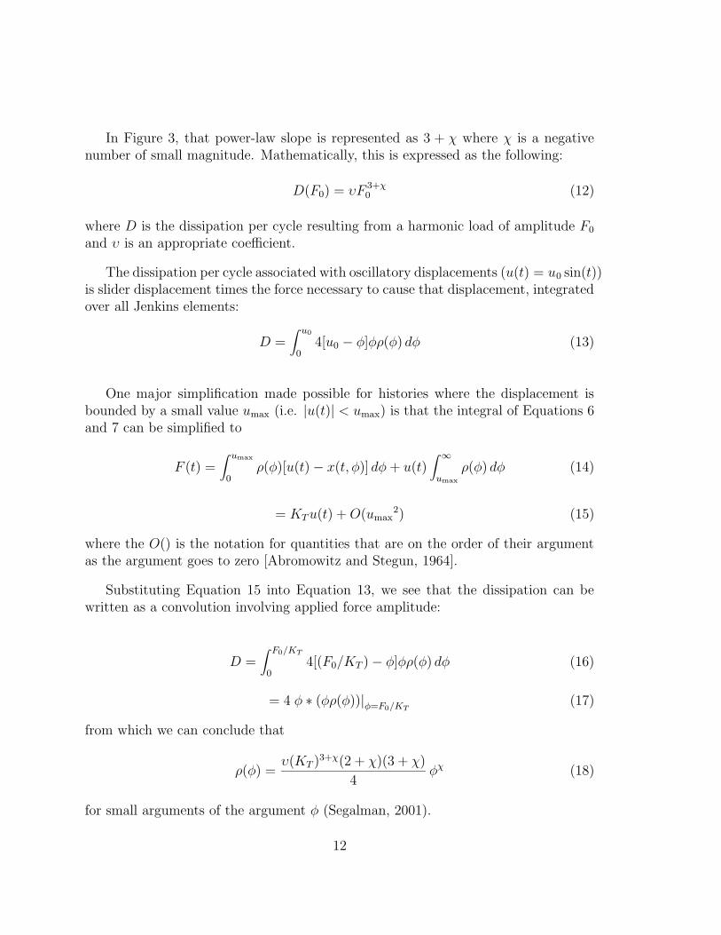
In Figure 3, that power-law slope is represented as 3 + χ where χ is a negativenumber of small magnitude. Mathematically, this is expressed as the following:

D(F0) = υF 3+χ0 (12)

where D is the dissipation per cycle resulting from a harmonic load of amplitude F0

and υ is an appropriate coefficient.

The dissipation per cycle associated with oscillatory displacements (u(t) = u0 sin(t))is slider displacement times the force necessary to cause that displacement, integratedover all Jenkins elements:

D =∫ u0

04[u0 − φ]φρ(φ) dφ (13)

One major simplification made possible for histories where the displacement isbounded by a small value umax (i.e. |u(t)| < umax) is that the integral of Equations 6and 7 can be simplified to

F (t) =∫ umax

0ρ(φ)[u(t) − x(t, φ)] dφ + u(t)

∫

∞

umax

ρ(φ) dφ (14)

= KT u(t) + O(umax2) (15)

where the O() is the notation for quantities that are on the order of their argumentas the argument goes to zero [Abromowitz and Stegun, 1964].

Substituting Equation 15 into Equation 13, we see that the dissipation can bewritten as a convolution involving applied force amplitude:

D =∫ F0/KT

04[(F0/KT ) − φ]φρ(φ) dφ (16)

= 4 φ ∗ (φρ(φ))|φ=F0/KT(17)

from which we can conclude that

ρ(φ) =υ(KT )3+χ(2 + χ)(3 + χ)

4φχ (18)

for small arguments of the argument φ (Segalman, 2001).

12

Log10(Force)

Log

10(D

issi

patio

n/C

ycle

)

slope=3

slope=

Figure 3. The dissipation resulting from small amplitudeharmonic loading tends to behave as a power of the force am-plitude.

13

Large Monotonic Loads

Let’s consider large monotonic pulls (0 < u). Equations 6 and 7 show that

F (t) =∫ u(t)

0φρ(φ)dφ + u(t)

∫

∞

u(t)ρ(φ)dφ (19)

from which Iwan derived∂2F (u)

∂u2= −ρ(u) (20)

Because the second derivative of force cannot be measured with any resolutionfor most joints at small displacements, the above is at best only useful for a large-displacement experiment.

Figure 4 sketches the monotonic force-displacement curve for a canonical lap joint.We anticipate that the force saturates fairly suddenly at FS and interface displacementuS. We envision the slope to be nearly discontinuous. Referring to Equation 20 weare inclined to expect that the density ρ(φ) has finite support and the character of aDirac delta at the positive end of that support.

Some comment should be made about why we have to guess at the force displace-ment curves for joints in structures such as we usually encounter. The key observationis that the interface mechanics cannot be viewed directly. The interface region is actedon by external loads through a large elastic region. Additionally, kinematic measure-ments are of the net displacements of that composite system. Particularly vexing isthat the elastic subsystem is generally much more compliant than the interface untilthe interface has been forced into the vicinity of macro-slip.

This insight is illustrated in Figure 5 showing the monotonic force-displacementcurves for a lap joint simulated with an extremely fine mesh. We see that the forceis almost linear in displacement until macro-slip suddenly occurs. The nearly linearregion is dominated by the compliance of the elastic part of the system; the responseof the interface is almost entirely obscured. Once the force is sufficient to causemacro-slip, it is the (near infinite) compliance of the interface which dominates. Theconclusion is that for our class of structures, it is very hard to achieve resolution onthe force-displacement response of the interface itself through measurements of elasticsystems of which the joint is only a small part.

It should be said that for some structures for which the joints represent a majorsource of stiffness degradation of the structure, Levine and White (2001) were ableto deduce Iwan parameters by examining distortion of nominal frequency response

14

Beginning of Macroslip

Pinning by Shank of Bolt

Microslip Regime

Forc

e

Displacement

(u ,F )S S

Figure 4. The monotonic pull of a simple lap joint showsthe force saturates at FS as the displacement passes a criticalvalue.

15

Figure 5. The numerical predictions of a finely meshedsystem containing a single lap joint illustrate how interfaceforce and displacements are obscured by the large complianceof the elastic response of the attached members.

16

curves as excitation frequency increased. This is an illustration of deducing jointproperties indirectly through observation of the integrated behavior of the full struc-tural dynamic response. It is through a similarly indirect approach that parameterestimation is pursued in the following.

Truncated Power-Law Spectra

Given the above observations, we are lead to consider parallel Iwan systems having apower-law population distribution terminated by a Dirac delta:

ρ(φ) = Rφχ[H(φ) − H(φ − φmax)] + Sδ(φ − φmax) (21)

where H() is the Heaviside step function and φmax is numerically equal to uS. Thecoefficient S has a value to bring the slope of the monotonic pull curve down to zeroat (us, Fs). This form of population distribution is shown graphically in Figure 6.

Substitution of Equation 21 into Equation 6 yields

F (t) =∫ φmax

0[u(t) − x(t, φ)]Rφχ dφ + S[u(t) − x(t, φmax)] (22)

Equation 7 remains unaltered.

The macro-slip force for the system becomes

FS =∫ φmax

0φρ(φ)dφ (23)

=Rφχ+2

max

(χ + 2)+ Sφmax (24)

= φmax

(

Rφχ+1max

χ + 1

)

[χ + 1

χ + 2+ β] (25)

where

β = S/

(

Rφmaxχ+1

χ + 1

)

(26)

Because χ and β are dimensionless and because FS can be measured or computedfairly directly, a preferred set of model parameters are {χ, β, FS, φmax}. For thisreason, one inverts Equation 25 to solve for R and employs Equation 26 to express Sappropriately:

17

��

��

��

��

��

��

φ

ρ(φ)

Figure 6. A spectrum that is the sum of a truncated powerlaw distribution and a Dirac delta function can be selectedto satisfy asymptotic behavior at small and large force ampli-tudes.

R =FS(χ + 1)

φχ+2max (β + χ+1

χ+2)

(27)

and

S =

(

FS

φmax

)

β

β +(

χ+1χ+2

)

(28)

The interface stiffness could be computed as

KT =∫ φmax

0ρ(φ)dφ =

Rφχ+1max

(χ + 1)+ S =

Rφχ+1max

(χ + 1)(1 + β) =

FS(1 + β)

φmax(β + χ+1χ+2

)(29)

Oscillatory Response

Because of signal-to-noise problems, there is little data available in the regime of smallimposed loads. We are left having to do parameter identification and comparisons

18

with data from experiments involving large-forces. In particular, we examine large-force oscillatory experiments.

Direct solution of Equations 22 and 7 for a problem specified by F = F0 sin(t)would involve solution of a difficult nonlinear integral equation. An alternative ap-proach is to specify u(t) = u0 sin(t) and then to solve for the resulting dissipation andpeak force.

Noting that the maximum displacement of Jenkins elements of strength φ isx(t, φ) = u0 − φ, we observe that for u0 ≤ φmax the dissipation per cycle of suchelements is 4(u0 − φ)φ. The net dissipation per cycle is

D =∫ u0

04[(u0 − x(t, φ))]φρ(φ)dφ (30)

This is similar to Equation 16, but no assumption of small displacement is made.For the density function of Equation 22 and for u0 ≤ φmax, the dissipation per cycleis

4Ru0χ+3

(χ + 3)(χ + 2)= rχ+3 4Rφmax

χ+3

(χ + 3)(χ + 2)= rχ+3 4FS φmax (χ + 1)

(β + χ+1χ+2

)(χ + 2)(χ + 3)(31)

where r = u0/φmax.

Next, we presume that the maximum force seen in each cycle is that force currentduring the maximum displacement in the cycle.

F0 =∫ u0

0φρ(φ)dφ + u0

∫ φmax

u0

ρ(φ)dφ (32)

= u0(S + Rφmax

χ+1

χ + 1) − Ru0

χ+2

(χ + 1)(χ + 2)(33)

Though the above is not a rigorously derived relationship, numerical calculations haveshown it to be correct to within numerical precision.

Equation 33 is made non-dimensional by dividing by FS

F0/FS = r(β + 1) − rχ+1/(χ + 2)

β + (χ + 1)/(χ + 2)(34)

The experimental quantity most easily measured is dissipation (D) as a functionof applied lateral load amplitude (F0). Though these are dimensioned quantities, we

19

see that all the dimensions drop out when we plot ∂ log(D)/∂ log(F0/FS)

∂ log(D)/∂ log(F0/FS) =∂D/∂u0

D/∂F0/∂u0

F0

(35)

= (χ + 3)(S + Rφmax

χ+1

χ+1) − R u0

χ+1

(χ+1)(χ+2)

(S + Rφmaxχ+1

χ+1) − Ru0

(χ+1)χ+1

(36)

= (χ + 3)(β + 1) − rχ+1/(χ + 2)

(β + 1 − rχ+1)(37)

Note that as u0 → 0,

• F0 → u0(β + 1)Rφmaxχ+1

χ+1= u0KT ,

• and ∂ log(D)/∂ log(F0) → χ + 3.

Also, u0 → φmax,

• F0 → FS,

• and ∂ log(D)/∂ log(F0) → (χ + 3)(β + χ+1χ+2

)/β.

In a similar manner, we use the chain rule to calculate the second derivative ofthe log-log plot:

∂2 log D

∂log(F0/FS)2=

∂∂r

∂ log D∂ log(F0/FS)

∂∂r

log(F0/FS)(38)

=r(χ+1) (β + 1) (χ + 1)2 (χ + 3)

[

(β + 1)(χ + 2) − r(χ+1)]

[β + 1 − r(χ+1)]3(χ + 2)2

(39)

Note that as β → ∞, the curvature goes to zero everywhere, but if β = 0, thenthe curvature goes to ∞ as r → 1. If β is nonzero, then the curvature is at leastbounded.

One last quantity that involves only measurable components on the left hand side,but does retain one dimensioned element on the right hand side is

20

D/FS = 4φmaxrχ+3

(χ + 3)

(χ + 1)/(χ + 2)

[β + (χ + 1)/(χ + 2)](40)

While Equations 37 and 39 have to do with the shape of the log(D) vs log(F0)curve, Equation 40 is useful in choosing model parameters to match actual values ofdissipation.

Identifying Parameters

Discussed next are two similar strategies for determining the parameters for the Iwansystem discussed above so as to reproduce available experimental data. The firstmethod is more intuitive, and should give some sense of the meaning of each modelparameter. The second is automated and more suited to processing multiple sets ofexperimental data.

One quantity that is assumed known is FS, through either experiment or finiteelement analysis. Additionally, it is assumed that dissipation D as a function ofapplied lateral load amplitude is known over a range of those load amplitudes.

Manual Method

The following strategy for estimating the remaining parameters involves a lot of op-erator interaction and ’eyeballing’, but it appears to be robust. The computationalparts are easily implemented in Excel.

1. Plot the experimental values for log(D) vs. log(F0/FS), and adjust χ and βso that plot of log(D) vs. log(F0/FS) from Equations 31 and 34 has the sameslope and curvature as the experimental curve.

This is facilitated by generating a column of values of r and correspondingcolumns of F0/FS (Eq. 33) and D/(Rφ3+χ

max) (Eq. 31) and normalizing thatcurve so that it lies near the experimental data. The user then adjusts χ and βuntil the curves appear to overlie. If the curvature appears to be approximatelyzero, choose β to be a number on the order of 10.

2. Employ Equation 34 to deduce the dimensionless displacement amplitude r =u0/φmax corresponding to some data point near the center of the experimentaldata.

21

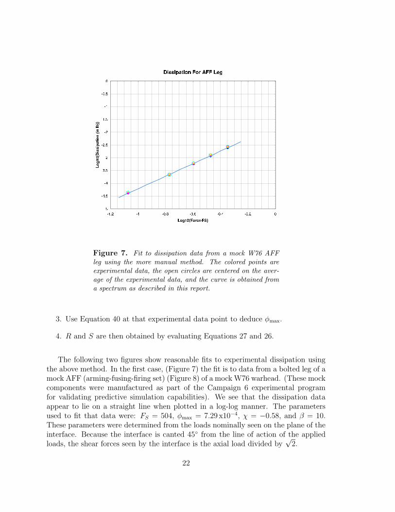
Figure 7. Fit to dissipation data from a mock W76 AFFleg using the more manual method. The colored points areexperimental data, the open circles are centered on the aver-age of the experimental data, and the curve is obtained froma spectrum as described in this report.

3. Use Equation 40 at that experimental data point to deduce φmax.

4. R and S are then obtained by evaluating Equations 27 and 26.

The following two figures show reasonable fits to experimental dissipation usingthe above method. In the first case, (Figure 7) the fit is to data from a bolted leg of amock AFF (arming-fusing-firing set) (Figure 8) of a mock W76 warhead. (These mockcomponents were manufactured as part of the Campaign 6 experimental programfor validating predictive simulation capabilities). We see that the dissipation dataappear to lie on a straight line when plotted in a log-log manner. The parametersused to fit that data were: FS = 504, φmax = 7.29 x10−4, χ = −0.58, and β = 10.These parameters were determined from the loads nominally seen on the plane of theinterface. Because the interface is canted 45◦ from the line of action of the appliedloads, the shear forces seen by the interface is the axial load divided by

√2.

22

��

��

Figure 8. The leg section of the AFF mock-up. To the leftis a finite-element mesh of the full leg section, in the middleis the actual leg section in the test apparatus, and to the rightis a sketch indicating the interface being modeled by the 4-parameter model.

23

Figure 9. Fit to dissipation data from a stepped specimen.The open circles are experimental data, and the curve is ob-tained from a spectrum as described in this report.

Though the AFF leg problem may appear simple (it is not) because the log-log plotof dissipation vs lateral force is nearly linear, the case of the stepped sample shownin Figure 9 shows substantially more curvature. This result is from a geometricallysimple test specimen (Figure 10). The qualitatively different response might be dueto the near singular normal tractions at the edges of the contact patch. Reasonablygood fit of the 4-parameter model presented above is obtained by setting FS = 400,φmax = 4.92 x10−5, χ = −0.6, and β = 0.1.

24

Figure 10. A stepped specimen shows qualitatively differentdissipation than a simple half-lap joint. The difference maybe do to the near singular traction that develop at the edgesof the contact patch.

25

Automated Method

Though the above algorithm might yield to automation, the following algorithm isdesigned especially to employ Matlab’s optimization tools. Matlab’s fminsearch toolis used to determine χ, β, and Rφχ+3

max so as to fit the experimental data points as wellas possible. One subtlety is that each comparison of the 4-parameter model with theexperimental data requires solution for r(χ, β, F0/FS). Once those three parametersare found, the rest of the steps are much as indicated in the previous method. Thenecessary code is illustrated in the Appendix .

Figures 11 and 12 illustrate the results of this method for the cases consideredabove. The parameters obtained by the method are indicated in those figures. We seethat in each case the more automated method (using Matlab) obtained parametersvery similar to those which were obtained in the more manual method, though theautomated method does reproduce the experimental data more closely.

Continuity of the Inverse Map

We have seen above that parameters can be found to make the 4-parameter modelreproduce experimental dissipation data reasonably well. A further measure of meritof a constitutive model is whether model parameters deduced to fit similar data setsare themselves similar. This issue is addressed here.

We consider dissipation data collected from an AFF leg nominally identical tothe one discussed above. The leg was repeatedly disassembled and reassembled andtested between disassembly/reassembly cycles. Nine resulting data sets are shown inFigure 13. We see that eight of those nine data sets lie reasonably close to each other.The data set labeled AFF 4 generates consistently less dissipation.

The Matlab code discussed above maps each data set to a set of four correspondingmodel parameters. Normalized model parameters deduced using the Matlab tool areshown in Figure 14. The value of FS is specified at the same value among all datasets, and the Matlab code tends to set β = 10 when there is little curvature inthe log(dissipation)/log(force) curve, so there is variation only in the χ and φmax

parameters. We see that the values of χ and φmax deduced from all the data setsseem to cluster with the exception of the valve of φmax deduced from data set AFF 4.

The anomalous nature of the fourth data set is illustrated more strongly by Figure15, where variability among the experimental data are considered. A variability metric

26

−1.4 −1.2 −1 −0.8 −0.6 −0.4 −0.2 0−5

−4.5

−4

−3.5

−3

−2.5

−2AFF Leg Number1, Sample Set 1: Dissipation Data

log10(F0/F

s)

log1

0(di

ssip

atio

n/cy

cle)

χ = −0.57505

β = 10φ

max = 0.00075856

Fs = 504

R = 580250.4699

S = 644820.1269

Resid = 0.0027019

Exit Flag = 0

Figure 11. Fit to dissipation data from a mock W76 AFFleg using the method exploiting Matlab.

27

Figure 12. Fit to dissipation data from a stepped specimenusing the method that employs Matlab.

28

Figure 13. Experimental dissipation curves measured for asingle mock AFF leg that was disassembled and reassembledbetween tests.

29

Figure 14. Parameters for the 4-parameter model deter-mined using Matlab code to fit the above experimental data.To show all parameters on one curve, each parameter wasnormalized by the average of the parameters deduced from alldata sets.

30

Figure 15. Variance (calculated using relative error) be-tween the 9 experimental data sets and the experimentalmean.

is defined here in a manner that captures the relative error:

V IE =

1

Ndata values

Ndata values∑

k=1

[

log(DIk/Dk)

]2(41)

where Dk is the kth data value averaged over all the data sets:

Dk =1

Ndata sets

Ndata sets∑

I=1

DIk (42)

and DIk is the kth data value in the Ith data set. We see that the variability of the

fourth data set stands out as being approximately ten times the next largest variabil-ity. From this point on, we discard that data set and consider only the remainingeight.

The model parameters obtained by averaging the corresponding parameters de-duced from each of the remaining eight data sets are reasonably close to those deduced

31

earlier for an AFF leg. They are χ = −0.57245, β = 10, φmax = 0.000761268, andFS = 504.

Figure 16 shows several measures of variability among the remaining eight datasets:

• The variability among the experimental data is shown on the left of the figure.In this case the largest variability is that of case AFF 7 and has a value ofapproximately 0.0025, corresponding to a disagreement between this data setand the average of the others of approximately 5%.

• The variability of the experimental data from the predictions made by themodel when each of the four model parameters is obtained by averaging thecorresponding parameters deduced from the eight experimental data sets:

V IM =

1

Ndata values

Ndata values∑

k=1

[

log(DIk/Dk)

]2(43)

where Dk is the kth data value predicted by the four-parameter model. We seethat the variability between the model predictions and the experimental data ison the same order as that found among the experimental data sets themselves.

• A more stringent test of the model’s ability to capture the experimental data isto measure the variability between each of the data sets and model predictionsmade using parameters deduced from all the other experimental data sets:

V IC =

1

Ndata values

Ndata values∑

k=1

[

log(DIk/D

Ik)]2

(44)

where DIk is the k data value predicted by the four-parameter model using model

parameters averaged from quantities deduced from all data sets except the Ith.We see that the variability between the model predictions and the experimentaldata is about 25% larger than that found among the experimental data setsthemselves. This is very good consistency.

We conclude from the above that the four-parameter model is capable both of repro-ducing the data provided to it and of doing so in a consistent manner with system-atically deducible parameters.

32

Figure 16. Variability (calculated using relative error)within the 8 clustering experimental data sets, between theexperimental data and that of the nominal model, and be-tween each data set and a model deduced using all the otherdata sets.

33

Power-Law Behavior

Some comment is appropriate about the determination of β (and φmax) for the casewhere the curvature of the log-log plot of dissipation versus force amplitude appearsto be zero. There is just not enough information in such cleanly power-law behaviorto determine the model parameters χ, β, and φmax. (FS should be known a pri-ori.) The following is done by both the manual and automated methods under thosecircumstances:

• β is automatically set to 10;

• χ is uniquely determined by the slope of the log-log dissipation curve;

• FS is known a priori;

• φmax is determined so that - consistent with the above values of χ, β, and FS -the predicted and measured dissipation are consistent.

If there are experimental or computational values for the stiffness of the systemcontaining that joint, the additional condition can be used to make the determina-tion of the model parameters better posed. In application, that last condition isimplemented by asking the Matlab optimization code to make the model stiffness KT

achieve the desired values.

For illustration we consider the AFF leg specimen again. In this instance wedevise an equivalent joint model for which all the forces and displacements occur indirection of the line of action of the applied force (Figure 17). Such a joint modelmight be used in a two degree-of-freedom approximation to a system consisting ofthe elastic portions of the specimen, the joint, and the reaction mass.

Resonance experiments indicate that the stiffness of the jointed leg is approx-imately 1.56x106 lbf/in. The stiffness of a similar monolithic (non-jointed) leg isapproximately 2.67x106 lbf/in. It would be desirable to be able to adjust β andφmax so that KT in Equation 29 could account for the difference. Alternatively onecould set the stiffness of the elastic component of the jointed structure to the full1.56x106 lbf/in and select β and φmax so that KT is substantially larger. In eithercase, we have guidance as to desirable ranges for KT . The first approach is demon-strated below.

34

��

��

��

Equivalent Joint

��

��

Figure 17. Idealized joint orthogonal to the line of actionof the applied forces: all joint forces and displacements arein the direction of the loads applied on the specimen.

35

If we choose to account for the softness of the jointed leg through the complianceof the joint, we find the joint stiffness to be

KT =1

(1/KJ) − (1/KM)=

1

(1/2.67x106) − (1/1.56x106)= 3.73x106 lbf/in (45)

Consideration of equilibrium shows the longitudinal force necessary to initiatemacro-slip in the joint is

FS = 504/ cos(45 deg) = 712 (46)

Similarly, the the log-log dissipation versus force amplitude curves used to find theremaining parameters employs longitudinal force amplitudes that are

√2 times the

force amplitudes seen on the actual interface surface. Application of the Matlab codewith and without reference to desired joint stiffness yields the parameters and fitshown in figure 18.

−1.4 −1.2 −1 −0.8 −0.6 −0.4 −0.2 0−5

−4.5

−4

−3.5

−3

−2.5

−2

AFF Leg Number1, Equiv. Longitudinal Model: KT Free

log10(F0/F

s)

log1

0(di

ssip

atio

n/cy

cle)

χ = −0.57566

β = 9.9712φ

max = 0.00053403

Fs = 712

R = 1347699.7151

S = 1294170.8531K

T = 1423961.2555

Resid = 0.0027023Exit Flag = 0

−1.4 −1.2 −1 −0.8 −0.6 −0.4 −0.2 0−5

−4.5

−4

−3.5

−3

−2.5

−2

AFF Leg Number1, Equiv. Longitudinal Model: KT Specified

log10(F0/F

s)

log1

0(di

ssip

atio

n/cy

cle)

χ = −0.62317

β = 3.659φ

max = 0.00022629

Fs = 712

R = 7123066.2368

S = 2925711.7917K

T = 3725311.9521

Resid = 0.0028176Exit Flag = 1

Figure 18. Model fit for an idealized joint orthogonal to theline of action of the applied forces. A constraint on joint stiff-ness is imposed in the calculations indicated on the right andno such constraint is imposed in the calculations indicated onthe left.

As expected, we see that the additional constraint does result in the desired jointstiffness but does not significantly change the quality of fit of the model predictionsto the experimental data points. Also as expected, though model parameters change,it is only β that changes significantly.

36

Discretization

Equations 6 and 7 are sufficient to solve for response of the above Iwan system onceone has all system parameters (R, χ, β, and φmax). It is useful to discretize theintegral in Equation 6 in the following manner. One breaks up the interval (0, φmax)into N intervals whose lengths form a geometric series:

∆φm+1 = α∆φm for all m + 1 < N (47)

where α is a number slightly greater than one (1 < α). That the sum of the intervalsmust be the whole interval:

N∑

m=1

∆φm = φmax (48)

permits us to solve∆φm = αm−1∆φ1 (49)

where

∆φ1 =[

φmaxα − 1

αN − 1

]

(50)

We consider one sample point, characterized by slide strength φm, at the mid-point of each interval ∆φm. At that sample point, the evolution of xm(t) is computedper Equation 7. For quadrature purposes, we refer to the coordinates of the left andright hand of each sub-interval as φl,m and φr,m respectively.

The force is evaluated by a discrete version of Equation 6.

F (t) =N∑

m=1

Fm(t) + Fδ(t) (51)

where

Fm(t) =

Rφ2+χ

r,m −φ2+χ

l,m

2+χsgn[u(t) − xm(t)] if ‖u(t) − xm(t)‖ = φm

Rφ1+χ

r,m −φ1+χ

l,m

1+χ[u(t) − xm(t)] if ‖u(t) − xm(t)‖ < φm

(52)

xm(t) evolves per Equation 2 where φ = φm,

Fδ = Sφmax[u(t) − xδ(t)], (53)

and xδ(t) evolves per Equation 2 where φ = φmax,

Note that the above quadrature reproduces the values for FS in Equation 24exactly.

37

The discretization discussed here is illustrated by the results of a C++ code thatimposes cyclic deformation on a four-parameter Iwan system and calculates the en-ergy dissipation once steady state is achieved (always on the second cycle). Thosenumerical calculations are compared with the analytic expressions of Equation 31. InFigure 19 we see that for the amplitude range 0.05FS < F0 < FS integration overthe responses of as few as ten Jenkins elements appears to be sufficient. We haveachieved satisfactory simulations in all exercises using values of α = 1.2 and N = 50.This is certainly overly conservative.

Figure 19. Comparison of dissipation prediction of Equa-tion 31 with the quadrature of Equations 51 through 53.

The question arises as to over how many Jenkins elements we really must integrate.The simplest criteria are

• in a monotonic pull, the stiffness degradation from KT down to zero at macro-slip should occur without too much discontinuity in the stiffness slope:

maxm

{ρ(φm)∆φm} ¿ KT (54)

where KT is evaluated from Equation 29. The maximum term in the above

38

sequence is that associated with the last increment, so the condition is

R

[

αN−1(1+α2

) − 1

αN − 1

]χαN−1(α − 1)

αN − 1φ1+χ

max ¿ KT (55)

For large N , the product on the left behaves as a constant times α − 1. Valuesof α on the order of 1.1 or 1.2 appear to cause Equation 55 to be satisfiedadequately.

• the sliding forces associated with the weakest element should slide at a forcewell below the smallest increment of force ∆Fmin between reversals that onewants to capture:

Rφ2+χ

r,1 − φ2+χl,1

2 + χ¿ ∆Fmin (56)

This becomes a condition that

R(

φmaxα − 1

αN − 1

)χ+2

/(χ + 2) ¿ ∆Fmin (57)

The quantity on the left goes as α−(χ+2)N , explaining why Equation 57 appearsto be satisfied with fairly modest values of N .

Conclusion

The four-parameter model presented here appears to be capable of capturing thedissipation behavior found from harmonically loaded experiments on lap-type jointsconducted so far. Further, the tools have been demonstrated to deduce the necessarymodel parameters with only modest effort.

Though the results presented here provide some reason for optimism, compari-son with more sophisticated experiments should be made. Among those experimentscould be multi-frequency experiments such as discussed by Segalman (2001) or ran-dom vibration experiments as performed by Smallwood for his hysteretic model. Eachof these classes of experiment has been explored by Smallwood(2001) in connectionwith his power-law hysteresis model.

Finally, one should note that constitutive equations of the sort developed hereare “whole-joint” models. Such models may capture the response of the joint forthe class of loads from which model parameters were deduced, but they give littleinsight into the micro-physics taking place. Over that longer term, more sophisticated

39

approaches must be developed that better incorporate the tractions and displacementsthat develop dynamically around the joint and that do not presume a specific natureto the joint loading. An effort into that new direction has been initiated.

40

References

[1] M. Abromowitz and I. A. Stegun, Handbook of Mathematical Functions, withFormulas, Graphs, and Mathematical Tables, p. 1045, 1964

[2] W. D. Iwan, A Distributed-Element Model for Hysteresis and Its Steady-StateDynamic Response, ASME Journal of Applied Mechanics, 33, pp. 893-900, 1966

[3] W. D. Iwan, On a Class of Models for the Yielding Behavior of Continuous andComposite Systems, ASME Journal of Applied Mechanics, 34, pp. 612-617, 1967.

[4] M. B. Levine and C. White, Microdynamic Analysis for Establishing NanometricStability Requirements of Jointed Precision Space Structures, Paper No. 325,Proceedings of the International Modal Analysis Conference Kissimmee Fl., Feb.2001.

[5] D. J. Segalman, An Initial Overview of Iwan Modeling for Mechanical Joints,SAND2001-0811, Sandia National Laboratories, Albuquerque, NM, March 2001.

[6] D. O. Smallwood, D. L. Gregory, and R. G. Coleman, A Three Parameter Con-stitutive Model for a Joint which Exhibits a Power Law Relationship BetweenEnergy Loss and Relative Displacement, 72nd Shock and Vibration Symposium,Destin FL, Nov. 2001. (Available from SAVIAC)

41

Example Matlab Files for Deducing Model Param-

eters

The following listings illustrate the automated approach to calculating model param-eters. The code is invoked by first entering the Matlab environment and then readingin a file containing the experimental data:

AFF1_1

and reading in the fitting code

find_param

where the data code AFF1.m would have the following form:

%fitting AFF leg

verbage = ’AFF Leg Number1, Sample Set 1: Dissipation Data’;

name = ’AFF1_1’;

disp(verbage);

D=[42.42640687 4.25E-05

84.85281374 2.13E-04

127.2792206 5.84E-04

169.7056275 1.23E-03

226.27417 2.56E-03];

Fs= 504;

and the Matlab code find param.m and the routines it calls are listed below.

43

find param.m

%This routine should be invoked only after the experimental data is ...

% read in. This version permits consideration of a desired

% stiffness K_T

force = D(:,1)/Fs;

Diss = D(:,2);

N = length(force);

% If K_T is not an input parameter, signal that it should be ignored

% in determining model parameters.

if(exist(’K_T’) <1),

K_T = -1;

end

% use optimizer to determine model parameters: \chi, \beta,

% \phi_max. R is output as well for convenience.

%

[chi,R,phi_max,beta,resid,flag]=fit3(D,Fs,K_T);

% Joint stiffness and S are calculated from the above parameters.

K_Tr = R*(phi_max^(chi+1))*(1+beta)/(chi+1);

S = beta*(R*phi_max^(chi+1))/(chi+1);

chi_name = ’\chi ’;

beta_name = ’\beta ’;

R_name = ’R ’;

S_name = ’S ’;

phi_max_name = ’\phi_{max}’;

Fs_name = ’F_s ’;

K_T_name = ’K_T’;

resid_name = ’Resid ’;

flag_name = ’Exit Flag’;;

chi_val = num2str(chi);

beta_val = num2str(beta);

R_val = num2str(R);

S_val = num2str(S);

phi_max_val = num2str(phi_max);

44

Fs_val = num2str(Fs);

K_T_val = num2str(K_Tr);

resid_val = num2str(resid);

flag_val = num2str(flag);

chi_val_Eq = [chi_name, ’ = ’, chi_val];

beta_val_Eq = [beta_name, ’ = ’, beta_val];

R_val_Eq = [R_name, ’ = ’, R_val];

S_val_Eq = [S_name, ’ = ’, S_val];

phi_max_val_Eq = [phi_max_name, ’ = ’, phi_max_val];

Fs_val_Eq = [Fs_name, ’ = ’, Fs_val];

K_T_val_Eq = [K_T_name, ’ = ’, K_T_val];

resid_val_Eq = [resid_name, ’ = ’, resid_val];

flag_val_Eq = [flag_name, ’ = ’, flag_val];

disp(chi_val_Eq);

disp(beta_val_Eq);

disp(R_val_Eq);

disp(S_val_Eq);

disp(phi_max_val_Eq);

disp(Fs_val_Eq);

disp(K_T_val_Eq);

disp(resid_val_Eq);

disp(flag_val_Eq);

% Plot these results

rmin = 0.8*find_r(force(1),chi,beta);

rmax= (find_r(force(N),chi,beta)+1)/2;

Points = 51;

for i=1:Points,

eps = (i-1)/(Points-1);

r(i) = rmin + eps*(rmax-rmin);

Fr(i) = r(i)*( (beta+1)-(r(i)^(chi+1))/(chi+2) )/ ...

( beta+(chi+1)/(chi+2) );

Dr(i) = 4*R*((r(i)*phi_max)^(chi+3))/( (chi+2)*(chi+3) );

end

%save these comparision data

comp_file_name = [name, ’.mat’];

45

eval([’save ’,comp_file_name,’ chi beta phi_max Fs force Diss Fr Dr ’]);

plot(log10(force),log10(Diss),’x’,log10(Fr), log10(Dr));

% axis( [log10(force(1)), log10(force(length(force))), ...

% log10(Diss(1)), log10(Diss(length(force)))])

title(verbage);

xlabel(’log10(F_0/F_s)’);

ylabel(’log10(dissipation/cycle)’);

text(0.7,0.5, chi_val_Eq, ’sc’);

text(0.7,0.45, beta_val_Eq, ’sc’);

text(0.7,0.40, phi_max_val_Eq,’sc’);

text(0.7,0.35, Fs_val_Eq, ’sc’);

text(0.7,0.25, R_val_Eq, ’sc’);

text(0.7,0.20, S_val_Eq, ’sc’);

text(0.7,0.15, K_T_val_Eq,’sc’);

text(0.7,0.05, resid_val_Eq,’sc’);

text(0.4,0.05, flag_val_Eq, ’sc’);

printname = [name,’.ps’];

eval([’print -dpsc ’,printname]);

outname = [name,’.out’];

fout = fopen(outname, ’w’);

%First Identify data set, then put out fitted values

fprintf(fout, ’\t%s\n’, name);

fprintf(fout, ’%s \t %s\n’, chi_name, chi_val);

fprintf(fout, ’%s \t %s\n’, beta_name, beta_val);

fprintf(fout, ’%s \t %s\n’, phi_max_name,phi_max_val);

fprintf(fout, ’%s \t %s\n’, Fs_name, Fs_val);

fprintf(fout, ’%s \t %s\n’, R_name, R_val);

fprintf(fout, ’%s \t %s\n’, S_name, S_val);

fprintf(fout, ’%s \t %s\n’, resid_name, resid_val);

fprintf(fout, ’%s \t %s\n’, flag_name, flag_val);

fprintf(fout, ’\n’);

fclose(fout);

46

fit3.m

%

% [chi,R,phi_max,beta,resid,flag]=fit3(Din,Fs,K_T);

%

% where Din = [force dissipation] (n x 2) matrix

% Fs = breakfree force

%

function [chi,R,phi_max,beta,resid,flag]=fit3(Din,Fs,K_T)

N = length(Din);

force = Din(:,1)/Fs;

Diss = Din(:,2);

% first guesses for parameters

chi = 0.0;

R = median(Diss);

phi_max = 1.0e-5;

beta =5;

if size(Din,1)<2,

disp(’pls provide at least 2 points’);

else

p=zeros(2*N+2,1);

% why is this dimensioned to N instead of 3

x=zeros(3,1);

for i=1:N,

p(i) = force(i);

p(i+N) = Diss(i);

end

p(2*N+1) = Fs;

p(2*N+2) = K_T;

x(1) = chi; % first guess for chi

x(2) = beta; % first guess for beta

x(3) = R; % first guess for R_p3c

options = optimset(’TolX’,1e-5,’Display’,’final’);

[x,resid,flag]=fminsearch(’para_fit3’,x,options,p);

chi = x(1);

47

beta = x(2);

R_p3c = x(3); %this should be R*phi_max^(chi+3)

r = zeros(N,1);

% estimate phi_max from each experimental data pair

pm = zeros(N,1);

for i=1:N,

r(i) = find_r(force(i), chi, beta);

pm(i) = (Diss(i)/Fs)*( (chi+3)*(beta+(chi+1)/(chi+2)) )/ ...

(4*(r(i)^(chi+3))*(chi+1)/(chi+2));

end

% average these to get a nominal phi_max

phi_max = sum(pm)/N;

R = R_p3c/phi_max^(chi+3);

end

48

para fit3.m

function [err]=para_fit3(x,p)

% there are N data points

N = floor(length(p)/2)-1;

F = zeros(N,1); % dimensionless force

D = zeros(N,1); % dissipation at each data point

r = zeros(N,1); % estimate for r corresponding to each F

for i=1:N,

F(i)=p(i);

D(i)=p(i+N);

end

Fs = p(2*N+1);

K_T = p(2*N+2);

chi = x(1);

beta = x(2);

R_p3c = x(3);

% for each data point force F and current values for chi & beta

% calculate the corresponding r

for i=1:N,

r(i) = find_r(F(i), chi, beta);

end

%calculate the corresponding dissipation

y=zeros(N,1);

for i=1:N,

y(i) = 4*R_p3c*(r(i)^(chi+3))/( (chi+2)*(chi+3) );

end

res = zeros(N,1);

for i=1:N,

% res(i) = (y(i)-D(i))/D(i);

res(i) = log10(y(i)/D(i));

end

49

%net residual

err = res’*res ;

% calculate stiffness

phi_max = (R_p3c/Fs)*(beta + (chi+1)/(chi+2))/(chi+1);

R = R_p3c/phi_max^(chi+3);

K_Tr = R*(phi_max^(chi+1))*(1+beta)/(chi+1);

if((1.0e-5< K_T) & (1<beta))

err = err + ((K_T - K_Tr)/K_T)^2;

end

%TEST TEST

%weight toward smaller magnitude chi

err = err + (5.0e-3)*chi*chi;

%Try to bound beta & chi

if(10<beta),

err = err + 1.0e3*(beta-10)^2;

end

if(beta<0.001),

err = err + 1.0e6*(beta-0.001)^2;

end

if(chi<-0.999),

err = err + 1.0e6*(chi+0.999)^2;

end

50

find r.m

%

% r = find_r(Ft,chi,beta);

%

% routine to find the r that results in a target value of Ft

%

function r = find_r(Ft, chi, beta)

%

%

% first estimate:

r = Ft;

%

% iteration parameters

i = 1; max_i = 100;

tol = 1.0e-4;

res = Ft;

while (i<max_i & Ft*tol<abs(res))

F = r*( (beta+1)-(r^(chi+1))/(chi+2) )/ ...

( beta+(chi+1)/(chi+2) );

res = F-Ft;

slope = ( (beta+1) - r^(chi+1) )/(beta + (chi+1)/(chi+2));

r = r - res/slope;

r = max(r, -1);

r = min(r, 1);

i = i+1;

end

51

DISTRIBUTION:

5 Prof. Lawrence A. BergmanUniversity of Illinois306 Talbot Lab104 S. Wright St.Urbana, IL 61801

1 Dr. Scott DoeblingLos Alamos National Labora-tory, MS P946Los Alamos, NM 87545

1 Dr. Steve GriffinBoeing SVS4411 The25 Way NESuite 350Albuquerque, NM 87109

1 Dr. Jason HinkleAerospace Engineering Sci-encesCampus Box 429University of ColoradoBoulder, CO 80309-0429

1 Prof. Raouf A. IbrahimCollege of Engineering2119 Engineering Bldg.Mechanical Engineering De-partmentWayne State UniversityDetroit, MI 48202

1 Dr. Marie Levine-WestJet Propulsion LaboratoryScience and Technology De-velopment Section4800 Oak Grove DrivePasadena, CA 91109-8099

1 Professor K. C. ParkCollege of Engineering andApplied ScienceUniversity of ColoradoBoulder, CO 80309-0429

1 Prof. Lee PetersonAerospace Engineering Sci-encesCampus Box 429University of ColoradoBoulder, CO 80309-0429

1 Dr. Chris PettitAFRL/VASD,Bldg. 146, 2210 Eighth St.,Wright Patterson AFBOH 45433

1 Prof. D. Dane QuinnDepartment of MechanicalEngineeringCollege of EngineeringThe University of Akron107b Auburn Science and En-gineering CenterAkron, OH 44325-3903

1 Dr. Y.C. YiuLockheed Martin Missiles &SpaceOrganization E4-20 Bldg 1541111 Lockheed Martin WaySunnyvale, CA 94089

1 MS 191Epp, David S , 9125

1 MS 191Ozdoganlar, O Burak ,9124

1 MS 553Bateman, Vesta I , 9126

52

1 MS 553Smallwood, David O , 9124

1 MS 555Garrett, Mark S , 9122

1 MS 555Gregory, Danny L , 9122

1 MS 555Hansche, Bruce D , 9122

1 MS 555Nelson, Curtis F , 9124

1 MS 555Nusser, Michael A , 9122

1 MS 557Baca, Thomas J , 9125

1 MS 557Carne, Thomas G , 9124

1 MS 557Larkin, Paul A , 9125

1 MS 557Mayes, Randall L , 9125

1 MS 557O’Gorman, Christian C ,9125

1 MS 557Paez, Thomas L , 9133

1 MS 557Simmermacher, Todd W ,9124

1 MS 557Urbina, Angel , 9133

1 MS 821Gritzo, Louis A , 9132

1 MS 824Moya, Jaime L , 9130

1 MS 824Ratzel, Arthur C , 9110

1 MS 828Pilch, Martin , 9133

1 MS 834Johannes, Justine E , 9114

1 MS 835McGlaun, J Michael , 9140

1 MS 835Naething, Richard M ,9142

1 MS 835Pierson, Kendall Hugh ,9142

1 MS 835Walsh, Timothy Francis ,9142

1 MS 841Bickel, Thomas C , 9100

1 MS 841Peterson, Carl W , 9100

1 MS 847Alvin, Kenneth F , 9124

1 MS 847Attaway, Stephen W , 9134

1 MS 847Bhardwaj, Manoj K , 9142

1 MS 847Bitsie, Fernando , 9124

53

1 MS 847Blanford, Mark L , 9142

1 MS 847Burchett, Steven N , 9126

1 MS 847Dohrmann, Clark R , 9124

1 MS 847Duong, Henry , 9126

1 MS 847Fulcher, Clay W G , 9125

1 MS 847Gwinn, Kenneth W , 9126

1 MS 847Heinstein, Martin W , 9142

1 MS 847Hinnerichs, Terry , 9126

1 MS 847Hopkins, Ronald N , 9125

1 MS 847Jung, Joseph , 9126

1 MS 847Lash, Joel , 9126

1 MS 847May, Rodney A , 9126

1 MS 847Mitchell, John A , 9142

1 MS 847Morgan, Harold S , 9120

1 MS 847Red-Horse, John R , 9133

1 MS 847Redmond, James M , 9124

1 MS 847Reese, Garth M , 9142

10 MS 847Segalman, Daniel J , 9124

1 MS 847Sumali, Hartono , 9124

1 MS 847Walther, Howard P , 9125

1 MS 847Wojtkiewicz, Steven F Jr ,9124

1 MS 893Brannon, Rebecca M ,9123

1 MS 893Lo, Chi , 9123

1 MS 893Reedy, Dave , 9123

1 MS 1110Day, David M. , 9214

1 MS 1023Stasiunas, Eric Carl , 9124

1 MS 1080Dohner, Jeffrey L, 1769

1 MS 1135Coleman, Ronald G , 9122

1 MS 1360Resor, Brian R , 9122

1 MS 1393Chu, Tze Yao , 9100

54

1 MS 9018Central Technical Files,8945-1

2 MS 0899Technical Library, 9616

1 MS 0612Review & Approval Desk,9612

55

a four-parameter iwan model for lap-type...

Documents