a fluorescent oil detection device - lsu digital commons

Louisiana State UniversityLSU Digital Commons

LSU Doctoral Dissertations Graduate School

2013

A fluorescent oil detection deviceYuxuan ZhouLouisiana State University and Agricultural and Mechanical College, [email protected]

Follow this and additional works at: https://digitalcommons.lsu.edu/gradschool_dissertations

Part of the Mechanical Engineering Commons

This Dissertation is brought to you for free and open access by the Graduate School at LSU Digital Commons. It has been accepted for inclusion inLSU Doctoral Dissertations by an authorized graduate school editor of LSU Digital Commons. For more information, please [email protected].

Recommended CitationZhou, Yuxuan, "A fluorescent oil detection device" (2013). LSU Doctoral Dissertations. 1895.https://digitalcommons.lsu.edu/gradschool_dissertations/1895

https://digitalcommons.lsu.edu?utm_source=digitalcommons.lsu.edu%2Fgradschool_dissertations%2F1895&utm_medium=PDF&utm_campaign=PDFCoverPages

https://digitalcommons.lsu.edu/gradschool_dissertations?utm_source=digitalcommons.lsu.edu%2Fgradschool_dissertations%2F1895&utm_medium=PDF&utm_campaign=PDFCoverPages

https://digitalcommons.lsu.edu/gradschool?utm_source=digitalcommons.lsu.edu%2Fgradschool_dissertations%2F1895&utm_medium=PDF&utm_campaign=PDFCoverPages

https://digitalcommons.lsu.edu/gradschool_dissertations?utm_source=digitalcommons.lsu.edu%2Fgradschool_dissertations%2F1895&utm_medium=PDF&utm_campaign=PDFCoverPages

http://network.bepress.com/hgg/discipline/293?utm_source=digitalcommons.lsu.edu%2Fgradschool_dissertations%2F1895&utm_medium=PDF&utm_campaign=PDFCoverPages

https://digitalcommons.lsu.edu/gradschool_dissertations/1895?utm_source=digitalcommons.lsu.edu%2Fgradschool_dissertations%2F1895&utm_medium=PDF&utm_campaign=PDFCoverPages

mailto:[email protected]

A FLUORESCENT OIL DETECTION DEVICE

A Dissertation

Submitted to the Graduate Faculty of theLouisiana State University and

Agricultural and Mechanical Collegein partial fulfillment of the

requirements for the degree ofDoctor of Philosophy

in

The Department of Mechanical Engineering

byYuxuan Zhou

B.S., Tsinghua University, P. R. China, 2006M.S., Louisiana State University, 2010

May 2013

ii

ACKNOWLEDGEMENTS

Several people have been instrumental in the completion of this project. First, I would

like to specially thank Dr. Wanjun Wang, my major professor, for providing me with his

extensive knowledge in microelectromechanical systems (MEMS) and microfabrication

technologies. His infinite guidance, patience, and encouragement made this thesis possible.

Furthermore, his academic manner and approach to problems will continue to influence me in

my future studies.

I would also like to thank my fellow graduate students. Their intelligent discussions and

valuable suggestions have helped me significantly throughout this project. Their friendship has

also made working in the laboratory a lifetime experience for me.

Finally, I am extremely grateful to my dearest parents for helping me believe in myself

and for encouraging me to pursue my doctoral degree in Mechanical Engineering. Their

guidance, blessings, and love have brought me a long way in my life.

iii

TABLE OF CONTENTS

ACKNOWLEDGEMENTS............................................................................................................ ii

TABLE OF CONTENTS............................................................................................................... iii

LIST OF TABLES.......................................................................................................................... v

LIST OF FIGURES ....................................................................................................................... vi

ABSTRACT................................................................................................................................. viii

CHAPTER 1. INTRODUCTION ................................................................................................... 11.1 A historical environmental disaster in the Gulf of Mexico.................................................. 11.2 Effect of the disaster............................................................................................................. 3

1.2.1 Short term effects.......................................................................................................... 31.2.2 Long-term effects ......................................................................................................... 4

1.3 Monitoring after spill is important ....................................................................................... 71.4 Oil components and detection technologies......................................................................... 91.5 The theory of fluorescence generation ............................................................................... 101.6 Oil fluorescence.................................................................................................................. 121.7 Current issues of fluorescence oil detection Instruments................................................... 131.8 MEMS application examples ............................................................................................. 141.9 The research goal and my contributions ............................................................................ 15

CHAPTER 2. DESIGN OF THE MICROCHIP AND FABRICATION TECHNOLOGY......... 182.1 General design of the micro-fluidic-optic chip .................................................................. 192.2 Fabrication technology....................................................................................................... 22

2.2.1 UV Lithography of SU-8............................................................................................ 222.2.2 PDMS molding process .............................................................................................. 252.2.3 Micro cast with the PDMS intermediate mold ........................................................... 272.2.4 PDMS to PDMS bonding ........................................................................................... 27

2.3 Summary ............................................................................................................................ 28

CHAPTER 3. MICRO OPTICAL DETECTION SYSTEM ........................................................ 303.1 Background Introduction ................................................................................................... 303.2 Introduction of fluorescent properties ................................................................................ 31

3.2.1 Fluorescence effect and molecular structures............................................................. 313.2.2 Background factors on the fluorescence..................................................................... 333.2.3 Fluorescence parameters............................................................................................. 35

a. The average life of the fluorescent molecules............................................................. 35b. Fluorescence efficiency .............................................................................................. 36c. Fluorescence intensity and spectral shape, bandwidth, peak position ........................ 37

3.2.4 A model of oil fluorescence in water.......................................................................... 383.3 Select supporting parts of the optical detection system ..................................................... 40

iv

3.4 Design and fabrication of micro-optical detection system in the microchip...................... 443.4.1 General design of micro-optical detection system in the microchip .......................... 443.4.2 General fabrication process of the vertical microlens ................................................ 453.4.3 Simulation of lens surface profile............................................................................... 493.4.4 Experimental results ................................................................................................... 52

a. Calibrate the relation between pressure and focal length of lens by experiments ...... 52b. Experimental results of the microlenses ..................................................................... 54c. Feasibility test of the optical detection unit ................................................................ 57

3.5 Conclusions ........................................................................................................................ 58

CHAPTER 4. THE PERISTALTIC MICROPUMP .................................................................... 594.1 Background and introduction ............................................................................................. 594.2 Design and fabrication of the peristaltic pump ................................................................. 63

4.2.1 General principle and design of the peristaltic pump ................................................. 634.2.2 Design of the flow channel ......................................................................................... 664.2.3 Fabrication of electromagnetically actuated valve ..................................................... 684.2.4 Experimental results of the electromagnetically actuated valve ................................ 71

4.3 Experimental results of the prototype peristaltic pump and discussions ........................... 734.4 Summary ............................................................................................................................ 75

CHAPTER 5. LIQUID-LIQUID EXTRATCTION SYSTEM AND EXPERTIMENTSRESULTS OF FINAL INTEGRATED DEVICE ................................................. 77

5.1 Background ........................................................................................................................ 775.2 Design and fabrication of L-L extraction system............................................................... 79

5.2.1 Principle and general design of the L-L extraction system ........................................ 795.2.2 Counter-current and co-current flow configuration of the L-L extraction layer and

interface stability........................................................................................................ 825.2.3 Material selection for L-L extraction layer: SU-8 or PDMS...................................... 87

a. Comparison of SU-8 and PDMS surface modification............................................... 87b. Comparison of SU-8 and PDMS fabrication .............................................................. 89c. Summary of comparison ............................................................................................. 90

5.2.4 Surface modification of the PDMS L-L extraction layer ........................................... 915.2.5 Fabrication of L-L extraction layer ............................................................................ 935.2.6 Simulation of L-L extraction layer extraction efficiency ........................................... 96

5.3 Experimental results of the integrated system and comparison of different fence sizedesigns................................................................................................................................ 98

5.4 Conclusions ...................................................................................................................... 103

CHAPTER 6. CONCLUSIONS ................................................................................................. 105

REFERENCES ........................................................................................................................... 107

VITA........................................................................................................................................... 114

v

LIST OF TABLES

Table 1.1 NOAA estimations of the percentage cleaned by using different strategies .................. 2

Table 2.1 Temperature steps of prebake ....................................................................................... 24

Table 2.2 Temperature steps of post bake .................................................................................... 25

Table 3.1 Experiment result of micro lens (diameter d =100μm, membrane thickness t= 10μm) 53

Table 3.2 Experiment result of micro lens (diameter d =600μm, membrane thickness t= 120μm)....................................................................................................................................................... 54

Table 4.1 The valve leakage with different length SU-8 cuboid under different pressure ........... 73

Table 4.2 The valve leakage with different length NOA73 cuboid under different pressure....... 73

vi

LIST OF FIGURES

Fig.1.1 Schematic diagram of electron energy level translation................................................... 11

Fig.1.2 MEMS market in 2005 [15].............................................................................................. 14

Fig.2.1 System schematic of the oil concentration detection device ............................................ 19

Fig.3.1 Schematic diagram of a microfluidic device integrated with fluorescence opticaldetection system............................................................................................................................ 40

Fig.3.2 Cured out-of-plane microlens filled with NOA 73........................................................... 46

Fig.3.3 Schematic diagram of no lens, one-membrane lens and two-membrane lens integratedwith the fiber at position 1 and 2 .................................................................................................. 46

Fig.3.4 Light beam focused by one-membrane lens (a) and two-membrane lens (b) .................. 48

Fig.3.5 Schematic diagram of micro lens fabrication process ...................................................... 48

Fig.3.6 Schematic diagram of the experimental set-up used to apply pressure to the PDMSchamber to create the microlenses ................................................................................................ 49

Fig.3.7 Schematic diagram of PDMS membrane deformation..................................................... 50

Fig.3.8 Simulation result of a 600μm rectangular PDMS film deformed under 250kPa ............. 51

Fig.3.9 Simulation result of a 600 m rectangular PDMS film deformed under 500kPa............ 52

Fig.3.10 Experimental results of the micro-optical detection system for different oil densities. a)1000 ppm; b) 500ppm; c) 100ppm; d) 50ppm; e) 10ppm; f) 1 ppm; g) measured response vs. oildensity ........................................................................................................................................... 57

Fig.4.1 (a) Schematic diagram of the peristaltic pump working principle; (b) Schematic diagramof the valve design ........................................................................................................................ 65

Fig.4.2 600μmx600μm cross-section channel design and just closing the channel pressuresimulation...................................................................................................................................... 67

Fig.4.3 600μmx1000μm cross-section channel design and just closing the channel pressuresimulation...................................................................................................................................... 67

Fig.4.4 Schematic diagram of the micro valve fabrication process .............................................. 69

vii

Fig.4.5 Flow chart of the controlling program............................................................................. 74

Fig.5.1 Schematic Diagram showing the multi-layer structure for L-L extraction and fluidiccontrol for in-situ detection........................................................................................................... 80

Fig.5.2 Schematic design diagrams of the top-view for the L-L extraction unit in counter-flowoperation ....................................................................................................................................... 81

Fig.5.3 Schematic diagrams of the liquid-liquid extractor in counter-current (a) and co-current (b)flows with physical separation...................................................................................................... 83

Fig.5.4 Comparison of mass flux and concentration distribution of the solute in the extractor inco-current and counter-current flows............................................................................................ 84

Fig.5.5 Pressure profile of the two-phase flow along the channel.............................................. 85

Fig.5.6 (a) the shape of the interface when the organic phase moves to the hydrophilic surface;(b) the shape of the interface when the aqueous phase moves to the hydrophobic surface.......... 86

Fig.5.7 Schematic diagram of the PDMS surface modification ................................................... 92

Fig.5.8 Schematic diagram of the fabrication process for the L-L extraction layer .................... 95

Fig.5.9 The relation between C/C0 and time in the first (a) and second (b) flow circle .............. 97

Fig.5.10 Oil concentration distribution of both organic and aqueous phase in the first and secondflow circle ..................................................................................................................................... 97

Fig.5.11 Experimental results of the integrated system a) 1ppm sample without L-L extraction; b)1ppm sample with fence wall of 200μm by 200μm micro-posts and gaps and counter flow L-Lextraction; c) 1ppm sample with fence wall of 200μm by 200μm micro-posts and gaps and co-current flow L-L extraction; d) 1ppm sample with fence wall with 150μm by 150μm micro-postsand 150μm gaps in counter flow extraction................................................................................ 101

Fig.5.12 Experimental results of the integrated micro-fluidic-optic chip: a) experimental resultsof sample with 50ppm oil concentration without extraction; b) experimental results of samplewith 50ppm oil concentration and counter flow extraction using fence wall formed with micro-posts with cross-sectional area of 200μm by 200μm and gaps of 200μm; c) experimental resultsof sample with 50ppm oil concentration using fence wall formed with micro-posts with cross-sectional area of 200μm by 200μm and gaps of 200μm and co-current flow extraction; d)experimental results of sample with 50ppm oil concentration, fence wall formed of micro-postswith cross-sectional area of 150μm by 150μm and gaps of 150μm, counter-current flowextraction..................................................................................................................................... 102

viii

ABSTRACT

On April 20th 2010, the largest offshore oil spill in U.S. history happened in the Gulf of

Mexico. It is estimated total more than 4 million barrels oil spilled to Gulf of Mexico. More than

two million gallons had been used. This had made the threat to coastal and sea ecosystem even

greater and long term. Real-time monitoring is also a critical topic for oil spill response. In-situ

monitoring devices are needed for rapid collection of real-time data.

A new generation of instruments for spilled oil detection is reported in this paper. The

main hypothesis in this research is that the sensitivity of the new instrument based on a micro-

fluidic-optic chip can be higher than its conventional sized counterparts. The adoption of the

micro-fluidic-optic chip helped to miniaturize the sample extraction unit and also to integrate the

optical detection on the same chip substrate. Only the monitoring and displaying unit and the

power supply were external to the micro-fluidic-optic chip. In this way, the micro-fluidic-optic

chip is replaceable and can be disposable. This also helps to eliminate the need for cleaning the

fluidic components, which may be very difficult in micro-scales because of surface tension and

flow resistances.

Liquid-Liquid extraction unit for sample pre-concentration and micro-optic components

for fluorescence detection are the key microfluidic components and have been designed and

fabricated on a single disposable chip.

In the Liquid-Liquid extraction system, different designs are compared and

electromagnetically actuated micro-valves and peristaltic pumps have been designed and

fabricated to control the aqueous sample fluid and the organic phase solution. In the micro-optic

detection system, different designs are compared and an out-of-plane lens was designed,

fabricated, and integrated to enhance the measurement sensitivity.

ix

The experimental results of the integrated system have proved that the liquid-liquid

extraction functioned very well and the overall measurement sensitivity of the system has been

increased more than six hundred percent. An overall oil detection sensitivity blow 1ppm has

been achieved. The research work presented in this dissertation has proved the feasibility of this

novel oil detection instrument based on micro-fluidic-optic chip. This detection system may also

be used for detection of other samples that can be measured based on fluoresce principles.

1

CHAPTER 1 INTRODUCTION

1.1 A historical environmental disaster in the Gulf of Mexico

In April 20th 2010, the largest offshore oil spill in U.S. history happened in the Gulf of

Mexico because of the offshore oil-drilling rig explosion. Before it was capped on July 15th, oil

leaked at a rate estimated between 35,000 and 60,000 barrels per day. Till the well was officially

sealed in September 10, 2010 using cement, the total amount of oil spilled into the Gulf of

Mexico was estimated to be about 4.9 million gallons, resulting in the largest accidental marine

oil spill in world history.

The enormous amount of spilled oil spread over a large area of the Gulf, and formed

large underwater plumes. Many strategies were used to help contain the leaked oil, which include

removing the oil from the surface by skimmer ships, burning oil slicks at water surface, placing

sand barriers at shorelines setting up containment booms to corral the spilled oil, and etc..

Among them, the primary strategy was to use dispersants to dissolve the floating oil on the

surface and large underwater plumes under water.

Dispersants are chemicals used to break patches of oil into small droplets. With the help

of ocean waves, these oil droplets can subsequently spread to larger area instead of concentrating

in a small area. The hope was that larger area would have greater environmental self-healing

capacity to expedite the recovery.

The dispersants used are of the Corexit family which is banned in the United Kingdom

because of its toxicity. Though the federal government has ordered BP to limit the dispersant

usage, it is estimated that more than two million gallons, a record amount of dispersants, had

been used [1].

2

Table 1.1 presents the NOAA estimation of the percentage of spilled oil cleaned by using

each of these strategies. There are three possible alternative estimations. However, there is plus

or minus 10% uncertainty in the total volume. [2]

Table 1.1 NOAA estimations of the percentage cleaned by using different strategies

Category Estimate Alternative 1 Alternative 2

Direct recovery from wellhead 17% 17% 17%

Burned at the surface 5% 5% 5%

Skimmed from the surface 3% 3% 3%

Chemically dispersed 8% 10% 6%

Naturally dispersed 16% 20% 12%

Evaporated or dissolved 25% 32% 18%

Residual remaining 26% 13% 39%

From Table 1.1, it can be seen that there is still about 10%-40% oil still remaining in

ocean.

3

During the two years after the April 20, 2010, the damage to the ecosystem in the Gulf of

Mexico and surrounding coastal regions has been dramatic. While the ultimate impact on people

and wildlife is beyond accurate account, the severity can be glimpsed from the numbers of killed

wild animals reported by government agencies, which represents only a small fraction of total

ecosystem damage. The ultimate toll on people and wildlife is still not fully understood.

1.2 Effect of the disaster

The accidental spilling of such large amount of oil as in the Gulf of Mexico is rare. But

small spills happen frequently. The total volume annually is nevertheless quite large, and

becomes a critical pollution issue. Canada and the United State have a system collecting the data

of spill events. Statistically, most oil spills events reported are more than 4000L. In Canada,

there are about on average 12 spills reports every day, and 100 spills reported in the US. There is

800 million tons of oil pollution worldwide each year. There are about 3 to 5 million

underground chemicals and petroleum storage depots in the United States, and an annual average

of about 1% of the warehouse will leak. Every year at least 500 to 10 million tons of oil get into

water system through various means across the world. Oil spill offshore oil platforms operating

sewage oil is estimated 50,000 tons at least a year; maritime accident oil spill volume is about

410,000 tons per year, total an estimated 100 per year to 2.6 million tons of oil into the sea of

maritime transport operations and accidents [3].

1.2.1 Short term effects

This disastrous event has both short-term and long-term effects on the environment.

Short-term effects became obvious quickly following the spill. Because the high concentration

oil floating and underwater plume, the wildlife are directly poisoned to death, and the great

number of deaths break the ecosystem chain. And it will require long time to rebuild. As reported

4

by the government, over 8200 birds, 1200 sea turtles, 150 marine mammals were collected. The

number of dead fishes was uncountable. Experience of the similar disasters in the past indicates

that mortality can be assumed to be four to 11 times higher than the number of dead bodies

collected.

1.2.2 Long-term effects

The degradation of oil follows certain steps. First, when the oil initially leaked out, it

would spread over the water and form a few millimeters thick layer of slick on the water surface.

UV radiation in sunlight may oxidize some of the components in oil, a phenomenon called

photolysis. The volatile components which were original in oil or created after the photolysis

would evaporate quickly.

Some components will dissolve into seawater, known as dissolution. Most of them are

low molecular weight compounds which are relatively toxic. This dissolution is small,

representing less than 1% of the spilled oil. It will quickly dilute and degrade.

Most part of the oil is still dispersed into water as mentioned before, either broken up by

waves or with the help of the dispersants. Normally, the waves break the oil into droplets of

0.01–1mm in diameters. With help of the dispersants, the droplets can be smaller. In such small

sizes, they can be spread to large area and exist in water for a long period of time until being

degraded by bacteria. The duration is affected by many factors in the environment and almost

unpredictable.

Sinking is another phenomenon that usually happens. Because of the waves and ocean

flow, there is large amount of clay or sand flowing in the seawater. They will carry the oil,

accumulate to tar balls, and finally sink to the seabed.

5

Degradation of the dispersed oil depends on its concentration. It was hoped that

dispersants can help the emulsion of oil spreading to larger area, and reducing the average

concentration. Lower concentration means less hazard and faster degradation. But under certain

sea conditions special emulsion may be formed. The droplets are incorporated into floating oil

and a viscous substance called mousse will be formed. It is high concentration oil gathering with

20–80% seawater content. Mousse formation and stability normally depends on the specific type

of oil. The high concentration oil of this substance means it will take a long time to degrade it

and the affected area will suffer long-term ecosystem damage [4].

Only two years after the spill in the Gulf of Mexico, the long-term effect is yet to be well

understood. But study of other similar spills may provide some clue, for example Exxon Valdez

oil spill in 1992. Some studies still show the track of the oil remaining in the seawater after the

disaster. Of course, the high temperature and sufficient sunshine in Gulf of Mexico may help the

oil degradation.

The degrading rate of the oil in the water is not linear. Some studies show that only the

early phases of transportation and transformation of the oil followed expectations [5]. After the

accident in 1989, about 40 to 45% of the oil left on 787 km of PWS beaches; after 3-5 years,

only about 2% remained in the same place [5]. It means the decaying rate of the oil was about –

0.87 /year (loss of 58% over a year), which fitted the expectation perfectly. And according to the

expectation, the oil concentration on the oil spill spot will reduce to harmless level in 2-10 years.

Of course, rebuilding the damaged ecosystem will take a much longer time. The evaluation of

the recovery of the ecosystem is still controversial.

The rates of dispersion and degradation change with time. In 1992, it was estimated that

806,000 kg oil was left on PWS beaches. A 2001 survey showed that 55,600 kg still remained on

6

the PWS beaches. It meant that from 1992 to 2001, the decaying rate was only about 0.22 to –

0.30 per year (20-26% loss over a year). Perfect degradation process requires proper disturbance,

oxygenation, and photolysis. They are all affected by many factors. Under severe conditions such

as in this case, the degradation rate can be unexpectedly low.

Under normal condition in seawater, the oil usually can persist for half a year. If with

favorable condition, it can be degraded to background levels much quicker. The highest

concentration levels of oil are usually found in the spill center area, immediately under slicks or

mussel where the oil is mixed into the water by waves or dispersants. For example, in Amoco

Cadiz spill, immediately after the disaster happened, the concentration was about 3-20μg/L

offshore, 2-200μg/L near shore, and up to 500μg/L in the estuaries. The spill happened on March

16th, 1978. The concentration on offshore decreased to background levels (2μg/L) by April, on

near shore was about mid-May, and in the estuaries was no later than September. All were

degraded under half a year. In the Argo Merchant case, the highest concentration could be as

high as 250μg/L when the spill just happened. In February, two months later, samples were

widely collected over Georges Bank at all depths, and the result by measuring concentration of

these samples showed that the level of oil had decrease to 10-100μg/L. Measurement five months

later showed continued decrease in concentration to 1-50μg/L. By winter, about a year after the

spill, the concentration had fallen to generally less than 1μg/L, with occasional higher value up to

1-8μg/L in some places.

Some grained gravel shores have natural protection from the disturbances by waves with

geomorphologic armoring by boulders and cobbles [6]. These places can be good sedimentary

refuges for oil suppressing degradation and persisting. Some of oil was trapped in these places

with mussel form. And these places happen to be where some wildlife feeding or laying eggs. By

7

this way, oil enters food chain with high concentration [7]. It was reported pink salmon embryos

were exposed and killed through at least 1993 by the high concentration oil protected by the

boulders and cobbles [8]. And other habitats including fish eggs and invertebrate predators (sea

otters, sea ducks, and shorebirds) are weathered [9].

Because there are few continuing long period investigations on persistence in sediments

after those critical spills, the data of the oil degradation track is scare. But there are still some

data which can be taken as a small fraction of the persistence. In the Florida spill, oil was

measured in sediments 12 years after the spill. In the Arrow spill, a study aimed to find out the

remaining effect of the spill 6 years after spill found that the oil concentration in sediments was

still as high as 10-25,000μg/g. While death clams are average 650μg/g of oil, living species were

found to have 150-350μg/g of oil in these sediments. For different species, the contamination of

oil is different; the long-term effect by the oil is different. In the same case, Periwinkles were

also found average only 12-18μg/g. Spartina alterniftora, one kind of marsh grass, showed the

surprisingly high contamination of about 15,000μg/g from six oiled sites. Its contamination is

near 70μg/g even in well-controlled regime. In the case of Metula oil spilled in the Strait of

Magellan in 1974, some researchers estimate the persistence of oil in sand and gravel beaches

could be 15-30 years, and over 100 years for sheltered tidal flats and marshes. As oil last a long

time in sediments and marsh, the impacts it brings to local ecosystems require to be further

studied. [10]

1.3 Monitoring after spill is important

Real-time monitoring of the efficiency of dispersant application is a critical topic for oil

spill response. According to the Special Monitoring Applied Response Technologies (SMART)

protocol developed by U.S. Coast Guard, NOAA, U.S. Environmental Protection Agency, etc.,

8

when dispersants are used during spill response, the Unified Command needs to know whether

the operation is effective in dispersing the oil. In-situ monitoring devices are needed for rapid

collection of real-time data to assist the Unified Command with decision-making during

dispersant applications. According to the SMART protocol, the monitoring technique may need

to provide the concentration of spilled oil at multiple depths.

Another important issue of great concern is the long-term effects of the spilled oil to the

coastal water system. After applying the chemical dispersants, not all crude oil will be dispersed;

some oil slicks not dispersed may enter the costal water and inland water system due to tides,

winds and waves. These oil slicks tend to form ‘oil in water’ emulsion. The spilled oil tends to

dissolve slower in sediments and marsh than in seawater, because it has good protection for oil

from disturbance, oxygenation, and photolysis as mentioned before. Along the north coast of the

Gulf of Mexico, there are vast areas of marshes and wetlands with low salinity. This makes it

more difficult for any oil in it to dissipate and dissolve. It is therefore very important to keep

monitoring the leaked oil in the coastal water system, especially wetlands, and gather valuable

information not only for the evaluation of the impact of this oil spill disaster, but also for

building up a database for future studies of the long term effect of spilled oil on the wetland

ecosystem. The oil concentration monitoring in the wetlands has certain specific requirements

compared with the commonly-used in-ocean detection. First, since the oil in the wetland water

system is expected to be only a small portion of the dispersed oil and oil concentration can be

further lowered due to ecosystem restoration effects such as bio-degradation, oil detector with

ultra-low detection limit and sensitivity are required. Secondly, wetland has a more complicated

topography and is less accessible for large equipment, a low cost; in-situ, portable, system is

therefore keenly needed for monitoring oil concentration in wetland water system.

9

1.4 Oil components and detection technologies

The hydrocarbons in crude oil are mostly paraffin, alkanes, cycloalkanes and, various

aromatic hydrocarbons; while the other organic compounds contain nitrogen, oxygen and sulfur,

and trace amounts of metals such as iron, nickel, copper and vanadium. The detail of each

component is introduced as follows.

General formula of paraffin is CnH2n+2, a straight- or branched-chain molecule that can be

gasses or liquids at room temperature, depending upon the molecules, for examples: methane,

ethane, propane, butane, isobutane, pentane, and hexane.

General formula of Aromatics is C6H5-Y (Y is a longer, straight molecule that connects to

the benzene ring), which is ringed structures with one or more rings containing six carbon atoms,

and alternating double and single bonds between the carbons. Typical examples are benzene,

naphthalene.

General formula of napthenes or cycloalkanes is CnH2n, it is ringed structures with one or

more rings containing only single bonds between the carbon atoms typically liquids at room

temperature. Typical examples include cyclohexane, and methyl cyclopentane.

General formula of other hydrocarbons alkenes is CnH2n. It is linear or branched chain

molecules containing one carbon-carbon double-bond, for examples: ethylene, butene. General

formula of isobutene diene and Alkynes is CnH2n-2, which is linear or branched chain molecules

containing two carbon-carbon double-bonds, such as acetylene and butadienes.

A wide variety of instrumental and non-instrumental techniques is currently used in the

analysis of oil hydrocarbons, which includes gas chromatography (GC), gas chromatography

mass spectrometry (GC– MS), high-performance liquid chromatography (HPLC), size-exclusion

HPLC, infrared spectroscopy (IR), supercritical fluid chromatography (SFC), thin-layer

10

chromatography (TLC), ultraviolet (UV) and fluorescence spectroscopy, isotope ratio mass

spectrometry, and gravimetric methods [11]. Fluorescence spectroscopy is one of the important

techniques for on-site detection.

1.5 The theory of fluorescence generation

Certain chemical substances absorb and store energy from the outside, then get into the

excited state. When they get back from the excited state to the ground state, the excessive

energy will radiate in the form of electromagnetic radiation, i.e., emitting light. This is so called

fluorescence. Fluorescence generation consists of three main processes, the molecular absorption

of light energy, stimulation, and inactivation.

Absorption: When light travels through the material, certain frequencies of light will be

absorbed and weakened. Because of the limited numbers and discontinuous energy levels of

atoms, molecules or ions can only absorb two-level difference between the same or its integer

multiple of the energy. For the absorption of light, it can only absorb photons of certain

frequencies:

1 0 /E E hv hc , (1-1)

where E1 is absorbance substances in the ground state energy level, E0 is higher energy level for

the absorbance material, h is Planck (Plank) constant, v is the frequency of the light, λ is the

wavelength of light, and c is the speed of light in vacuum.

Excitation: When the material absorbs the radiation of a certain frequency, the electron

jumps from the ground state to the different vibrational levels of excited states, this process is

known as excitation.

11

Fig.1.1 Schematic diagram of electron energy level translation

Deactivation of the excited state molecule: Molecule in the excited state is unstable. It

will lose excessive energy and return to the ground state by the irradiative transition or non-

irradiative transition deactivation process. Molecular level transition diagram is shown in Figure

1.1. When the appropriate wavelength of the excitation light is irradiated at a molecule, the

irradiated molecule can absorb light and be excited to either level S1 or level S2. If the molecule

does not undergo chemical decomposition, it usually returns quickly to the first excited states of

the lowest energy level (Figure 1.1 S1 V0 level), this process does not contain the radiation of

light. The molecules on energy levels of the S1 (V0) are still unstable and will lose energy back

to the ground state of the S0 [12].

Therefore, the occurrence of the fluorescence has two necessary conditions: the first one

is the molecule of the substance must have the same characteristic frequencies with those of the

12

irradiation light. Molecule’s characteristic frequencies are closely related to their structures. The

occurrence of fluorescence must have an absorption structure. The second necessary condition is

that the molecules must have high fluorescence efficiency. Absorbance material does not

necessarily generate fluorescence if fluorescence efficiency may be too low, which is resulted

from the absorbed energy consumption by collisions between the solvent molecules or solute

molecules.

Excitation spectra: When an excitation monochromator is used, a fixed emission

wavelength is scanned and radiated on the fluorescent material, light with different wavelengths

are then excited. The fluorescence light generated by the fixed wavelength of the emission light

is collected and passed to the detector to detect the corresponding fluorescence intensity. The

curve of fluorescence intensity of the excitation wavelength can be recorded. Excitation spectra

can be taken as identification of fluorescent material or record of appropriate choice of excitation

wavelength during the fluorescence.

Emitting spectra: With the excitation light emission from the monochromator is scanned

across a given range, the fluorescence intensity of each wavelength from the testing substance

material corresponding to each excitation wavelength is measured and recorded. The recorded

relation between fluorescence intensity and emitting wavelength is plotted and named as “the

curve of the fluorescence spectra”. This property can be taken as the identification of fluorescent

material.

1.6 Oil fluorescence

Almost all kinds of substances can absorb UV or visible light, but only a few compounds

are fluorescent. Most of the fluorescent organic compounds contain aromatic rings, but not all of

the aromatic compounds are fluorescence. Crude oil mainly contains alkanes, cycloalkanes and

13

aromatic hydrocarbons. Aromatics and their derivatives are oil fluorescence sources on which

fluorescence spectrometry for measurement and identification is relied. Aromatic hydrocarbon is

25% to 70% of the total hydrocarbons of the oil, in which aromatic compounds containing

conjugated double bond compounds are dominant. These compounds include benzene,

naphthalene, anthracene, phenanthrene, fluoranthene, benzopyrene and other polycyclic aromatic

hydrocarbons and their derivatives, and porphyrin compounds containing heavy metals. They all

have unsaturated and π- electron conjugated structure and are the material bases of fluorescence

detection for oil and its derivatives.

1.7 Current issues of fluorescence oil detection Instruments

Operators from the US Coast Guard Strike Teams have found problems during the

operation of the Turner-10AU field portable Fluorometer (T-10AU) [13], which has been widely

used in oil detection [14]. The device is bulky (13.39 in. 21.65 in., weight – 34.5 lbs) and

requires various accessories such as pump cables, power supply etc. The current standardization

procedure for the Turner requires a standard fluoresce dye solution with large volumes.

Replacement and repair of the instrument can be very expensive. The system is quite complex to

operate and has poor sensitivity at lower density of oil. Because the instrument does not have an

integrated sample extraction unit, sample has to be pre-processed manually using an external

extraction kit (with a pipette, syringe, and additional volumetric glassware) to increase the oil

density of the sample first, and then measured based on fluorescence detection principle. This

increases the operation time and makes it difficult to operate, less portable, and therefore cannot

be used as an in-situ detection tool. According to SMART Protocol [14], a new generation

device is required.

14

1.8 MEMS application examples

Miniaturization and integration is the developing direction of the new generation device.

Miniaturization in electrical and sensor applications brings smaller devices with stronger

performance. Miniaturization and integration has become the feature of modern life. Many

modern devices are the application examples of the miniaturization and integration technology.

Silicon-based micro-electro-mechanical systems (MEMS) are one of the most promising

technologies in recent years. Fig.1.2 shows the major MEMS market in 2005 [15]. There are two

major applications for MEMS devices, one is the actuation devices (actuators) such as Ink Jet

Printer head or micro mirror device for projector, the other type includes all kinds of sensors.

The market for microfabricated sensors has been growing exponentially. However each sensor

application has its own specialties. Appropriate requirements, total performances of the system

and the combination of other components have to be well considered depending on each

application.

Fig.1.2 MEMS market in 2005 [15]

For current sensor applications, high precision and stability are limitations as the devices

become ever smaller [16]. When sensor package sizes become smaller, noise density level

becomes proportionally higher. Take the accelerometer as an example [15]:

2 2TNEA BNEA CNEA , (1-2)

15

where TNEA is total noise density equivalent acceleration, BNEA is Brownian noise equivalent

acceleration, CNEA is Circuit noise equivalent acceleration from IC circuit.

4 Bk TDBNEA

M

, (1-3)

and

CCNEA

S

, (1-4)

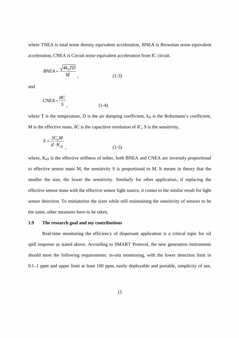
where T is the temperature, D is the air damping coefficient, kB is the Boltzmann’s coefficient,

M is the effective mass, δC is the capacitive resolution of IC, S is the sensitivity,

02

eff

C MS

d K , (1-5)

where, Keff is the effective stiffness of tether, both BNEA and CNEA are inversely proportional

to effective sensor mass M, the sensitivity S is proportional to M. It means in theory that the

smaller the size, the lower the sensitivity. Similarly for other application, if replacing the

effective sensor mass with the effective sensor light source, it comes to the similar result for light

sensor detection. To miniaturize the sizes while still maintaining the sensitivity of sensors to be

the same, other measures have to be taken.

1.9 The research goal and my contributions

Real-time monitoring the efficiency of dispersant application is a critical topic for oil

spill response as stated above. According to SMART Protocol, the new generation instruments

should meet the following requirements: in-situ monitoring, with the lower detection limit in

0.1–1 ppm and upper limit at least 100 ppm, easily deployable and portable, simplicity of use,

16

high reliability and easier logistics, less maintenance and lower maintenance costs, and capable

of being integrated with Windows operating systems and GPS.

A new technology for improved detection associated with oil spills is developed and a

novel MEMS detection device is presented in this dissertation. The goal is to develop a highly

sensitive and handheld instrument that can be used for in-situ detection of spilled oil. The device

needs to have much higher sensitivity, lower cost, easier to operate and maintain, and with

smaller size compared with the existing technologies. The applications of the instrument are not

limited to oil detection and may also be used to measure any organic samples that can be

measured in fluoresce detection principle.

The instrument is designed to have a built-in sample extraction/pre-concentration

function to eliminate external sample preparation kit. The oil detection is based on fluoresce

detection principle. In its heart is a disposable micro-sized detection cartridge with a built-in oil

pre-concentration unit. It will also contain a micro-sized optic detection unit consisting of

microlenses, micro-chamber for detection, and holders for optical fibers. The optic detection unit

will be integrated on the same substrate as the sample pre-concentration to form an integrated

micro-fluidic-optic detection cartridge. All the components on the cartridge will be passive with

no power supply requirement. This micro-cartridge can be replaced easily and can be disposable.

All the active components such as UV light source, photodetector, power supplies, etc., are

outside the cartridge and thus, do not require replacement for each test. The micro-cartridge can

be easily interfaced to these active elements. The micro-cartridge can be inexpensively fabricated

through mass production using micro-replication method. It can potentially be disposable and

eliminates the problem of cleaning and contamination as in permanently assembled fluidic

devices. The components and test the device first on a small dimension bench top model to

17

demonstrate feasibility and then in the next step, assemble and design a hand held device from

the tested bench top components for the implementation of a beta model.

18

CHAPTER 2 DESIGN OF THE MICROCHIP AND FABRICATIONTECHNOLOGY

In this chapter, the general design of the proposed instrument based on fluidic microchip

will be presented. The micro-fluidic-optic chip can be divided into three parts: an optical

detection system, a peristaltic micropump and a liquid-to-liquid (L-L) extraction microfluidic

system. All related fabrication technologies are introduced in detail in the following chapters.

From the discussion in Chapter 1, a new generation of instruments for spilled oil

detection is needed. The new generation instrument should meet the following requirements:

1) With the in-situ sensing capability;

2) Satisfactory detection limits. The lower detection limit should be within 0.1 – 1 ppm

and upper detection limit is at least 100 ppm;

3) Easily deployable and portable;

4) Simplicity of use. It should be simpler to operate than Turner, i.e., be easier to set up

and standardize;

5) High reliability –New instrument must be robust since turner setup may vary from day

to day and is sensitive to rough handling;

6) Easier Logistics – New instrument must have fewer components and must be lighter

and require less logistics than the current system that requires two large boxes weighing 75-100

lbs each;

7) Requiring less maintenance and lower maintenance costs;

8) Capable of being integrated with Windows operating systems and GPS.

The key point in miniaturizing the physical sizes while still maintaining the sensitivity of

sensors is to miniaturize the extraction processing and also to integrate the extraction and

19

detection on the same chip substrate. Only the monitoring and displaying unit, the power supply,

and other parts need to be external. In this way, the sample handling and sensing units will be

integrated on the chip itself and can be used as an independent and replaceable detecting head.

There will only be a cable between the detection chip and the supporting unit (power supply and

displaying). Another advantage is that one supporting unit can be used for several chips at the

same time.

2.1 General design of the micro-fluidic-optic chip

The schematic design diagram of the in-situ oil detection instrument is shown in Fig.2.1.

It includes two parts: microchip part (shown as yellow color) and supporting part (shown as grey

color). The microchip is designed as a replaceable cartridge to avoid cleaning after use. The

microchip can be replicated using micro-molding technology to save fabrication cost. It mainly

includes three key microfluidic components, which are the liquid-liquid (L-L) extraction system,

the micro optical detection system and the passive part of the peristaltic micropumps. The

peristaltic micropump is specially designed and fabricated. The actuators of the peristaltic pump

are designed to be right above the surface of the microchip, but not physically connected to the

remaining part of the fluidic microchip. The actuators of the micro pump will have long working

life. The rest microfluidic part of the pump is integrated in the microchip.

Fig.2.1 System schematic of the oil concentration detection device

20

The operational principle of microchip is as follows. First the sample aqueous solution is

imported into the microchip and pre-concentrated. The sample extraction/pre-concentration is

based on a liquid-to-liquid (L-L) extraction principle, also named solvent extraction and

partitioning. It is a technology commonly used in chemical engineering and other industries. The

technology can be used to separate compounds, such as oil, based on their relative solubility in

two different immiscible liquids, usually water and an organic solvent. It is therefore the most

natural option for the system for extraction of the oil from the aqueous sample solution into an

organic solvent, and then measured. In our design, the imported aqueous phase is extracted by an

organic phase. Many researchers have proposed sandwich-structured microfluidic devices for L-

L extraction applications [17-19]. In these designs, a porous hydrophobic membrane often used

to separate the two flow phases. But in our application, the oil is not dispersed as solution, but

emulsion. The droplet size of the oil is in the range 5m-150m. While the capillaries on the

porous membrane are much smaller than that, it is about 1m diameter. Therefore, a vertical

fence wall is used in our design. To keep the stability of interface of the two flows, the fence

wall will be selective surface modified.

The aqueous phase passed through one side of the L-L extraction continuously driven by

an external pump. To increase the concentration of oil in the organic phase, it is designed

flowing circularly on the other side of the L-L extraction system, so that the oil content in the

organic phase can accumulate as the aqueous phase solution passes by. The peristaltic pump is

almost the only option for both circular flow and separated actuators from the microfluidic

system requirements. Many different designs for peristaltic micropumps have been reported [20-

22]. But in these reports, the power of the actuators used is so weak that they can only drive flow

in very shallow channels (5m-10m). In our applications, the channels are as deep as 600m

21

and more powerful electromagnetic actuators are therefore needed. On the other hand, most

researchers designed the micropumps on the same substrate as the microfluidic chip. The micro

pumps and the microfluidic systems are therefore not separated. In this dissertation, a new design

of peristaltic micro pump is presented, in which the actuators are isolated from the microfluidic

system. In this design approach, the micropumps can be designed to have long working life but

the microfluidic chip is designed to be disposable

The pre-concentrated sample is then supplied to the fluorescence detection unit on the

same substrate for measurement. The micro-optical detection system has an integrated microlens

to boast the signal strength for improved sensitivity. Because of fabrication difficulty, most of

the reported microlenses are the in-plane ones [23-25]. Fabrication of the out-of-plane

microlenses is a critical problem because in most optical platforms, light transits in parallel with

the substrates of the systems. A new fabrication process for the out-of-plane microlenses with

controllable focal length is presented in Chapter 3. Components in grey color are supporting

parts outside the microchip. The supporting components can be divided to three parts by their

functions as shown in Fig.2.1. These supporting components, such as the monitoring and

displaying unit, the power supply, and other parts, will be assembled using commercial products.

Our goal was to develop a portable, easy to operate instrument with high sensitivity. Because the

size of the microchip is much smaller than those of the supporting components, the size of the

final instrument is primarily determined by the sizes of the supporting components. Sample

acquisition and filtration was done in an off-chip manner. Syringe with filter was used to obtain

sample from the testing point and deliver it into the on-chip sample reservoir. Other than this

sample acquisition, other fluid handling procedures are finished by on-chip micro-fluidic

components controlled by the peripheral electronic user interface. In the final instrument, there

22

will only be a cable between the detection chip and the supporting unit. The microchip and

supporting parts are only connected with a pair of cable connectors. Therefore, the microchip can

be independent and disposable but the supporting parts are the permanent parts of the instrument.

2.2 Fabrication technology

The fabrication of the micro-fluidic-optic oil detection chip was achieved using the

combination of some of the common micro fabrication technologies, such as UV lithography of

SU-8, PDMS molding process, micro cast with the PDMS intermediate mold, and PDMS to

PDMS bonding. The detailed fabrication procedure is presented in the next several chapters. In

this section, only the fundamental concepts will be introduced.

2.2.1 UV Lithography of SU-8

SU-8 is a negative resist commonly used in fabrication of high aspect ratio

microstructures and devices. As a negative photoresist, when it is exposed to ultraviolet light,

the exposed regions get cured and will remain after development while the unexposed regions

are removed. It is also known for its excellent UV lithography properties and widely used in the

fabrication of high aspect ratio microstructures and devices [26-28]. In addition, the exposed

(and cured) SU-8 polymer has excellent physical and chemical properties, and is highly resistant

to most chemicals and very stable in high temperature. Because of these advantages, UV

lithography of SU-8 is one of the key technologies used in fabricating the spilled oil detection

system presented in this dissertation. To explain how the technology is used, we will use the

fabrication of high aspect ratio micro-columns as the example here. The basic fabrication

process is as follows:

1. Wafer Cleaning. Clean up the wafer with water and acetone. After cleaning, the wafer is

then heated up to 80 degree centigrade for more than 1 hour to evaporate water.

23

2. Resist coating. SU-8 resist, especially the SU-8 50 and 100 as used in our work, has high

viscosity, therefore flows very slowly once poured on the wafer. Un-exposed SU-8 resist

can be easily removed with solvents such as acetone or SU-8 developer (provided by

MicroChem Corp.). The thickness of SU-8 resist depends on factors such as the viscosity

of SU-8, spinning time and speed. The relationship curves between the resist thickness and

these factors are readily found from the data sheets provided by the vendor of the resist,

Microchem Corporation

3. Prebake. The purpose of prebake is to evaporate the solvent from SU-8 resist. The

backside of wafer needs to be carefully cleaned with acetone to prevent the wafer from to

be stuck on the hot-plate during baking process. Big bubbles also need to be removed

before pre-bake, otherwise air will be trapped in the resist and remain inside the resist after

bake. Smaller bubbles can normally be removed during the pre-baking process. After

prebaking, SU-8 becomes a solid layer on the wafer. The prebaking temperature has to be

carefully controlled to prevent any residual stress in the resist and to achieve satisfactory

lithography results. The relationship of temperature-time is shown in table 2.1. The only

variable parameter is the dwelling time at 110℃. Generally, it is proportional to the

thickness of the SU-8. For example it takes 6 hours for a resist of 600μm and take 4 hours

for resist with thickness of 400μm. The ramping and dwelling times before and after the

maximum temperature are chosen to slow down the temperature rising up and dropping

down to reduce internal stress.

4. Preparation of lithography masks. The mask used in lithography is a piece of glass with

desired patterns, which are normally made of a thin layer of chrome. The commonly used

method of making mask is as follows: On one side of the glass, a thin layer of chrome is

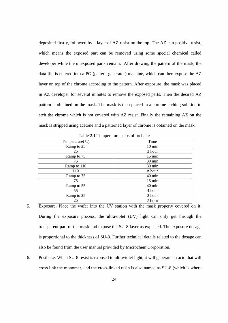
24

deposited firstly, followed by a layer of AZ resist on the top. The AZ is a positive resist,

which means the exposed part can be removed using some special chemical called

developer while the unexposed parts remain. After drawing the pattern of the mask, the

data file is entered into a PG (pattern generator) machine, which can then expose the AZ

layer on top of the chrome according to the pattern. After exposure, the mask was placed

in AZ developer for several minutes to remove the exposed parts. Then the desired AZ

pattern is obtained on the mask. The mask is then placed in a chrome-etching solution to

etch the chrome which is not covered with AZ resist. Finally the remaining AZ on the

mask is stripped using acetone and a patterned layer of chrome is obtained on the mask.

Table 2.1 Temperature steps of prebakeTemperature( C̊) Time

Ramp to 25 10 min25 2 hour

Ramp to 75 15 min75 30 min

Ramp to 110 30 min110 n hour



Ramp to 25 3 hour25 2 hour

5. Exposure. Place the wafer into the UV station with the mask properly covered on it.

During the exposure process, the ultraviolet (UV) light can only get through the

transparent part of the mask and expose the SU-8 layer as expected. The exposure dosage

is proportional to the thickness of SU-8. Further technical details related to the dosage can

also be found from the user manual provided by Microchem Corporation.

6. Postbake. When SU-8 resist is exposed to ultraviolet light, it will generate an acid that will

cross link the monomer, and the cross-linked resin is also named as SU-8 (which is where

25

the SU-8 got its name). After the UV exposure, the exposed wafer coated with SU-8

needs to be post-baked to improve the cross-link process, enhance the lithography quality,

and minimize possible residual stress. The temperature set is show in table 2.2.

Table 2.2 Temperature steps of post bakeTemperature ( ̊C) Time






Ramp to 25 30 min25 10 in

7. Development. After the post bake, the cross-link in SU-8 is almost completed, which

means the SU-8 developer now can only remove the unexposed parts but not exposed

parts. The development may take a longer time if the exposed wafer is placed in facing up

position in developer. When the wafer is placed in the “facing-down” position (with the

SU-8 side facing down vertically), the gravity helps to enhance the development process

by allowing the developed chemicals to drop off and improve the circulation. The

developed wafer needs to be carefully and slowly taken out from the developer to prevent

them from mechanical damages caused by the developer fluid.

2.2.2 PDMS molding process

PDMS (Sylgard 184 Dow Corning) can be used in a molding process to make an

intermediate negative pattern, which comes from a SU-8 master mold. The SU-8 master mold

can be prepared by using SU-8 lithography process as introduced in section 2.2.1

The detailed steps of PDMS molding process are as follow:

26

1. Preparation of the PDMS mixture. The vendor of the PDMS pre-polymers offers two pre-

polymer fluids, the base and the curing agent. They are usually mixed in a ratio of 10:1. If

the base in the mixture ratio is increased, the final PDMS polymer would be softer. On

the other hand, increasing the percentage of the curing agent would make the solidified

PDMS harder. Therefore the exact ratio of the base and curing agent can be adjusted as

needed to obtain the desired physical properties of the final PDMS polymers for different

applications.

2. Stirring. The mixture of the base and curing agent needs to be stirred for several minutes

to ensure complete mixing. The mixture can then be poured on the SU-8 master mold to

form a certain thickness of PDMS layer. The thickness can be controlled by manipulating

the weight of PDMS.

3. Eliminate the air bubbles. The wafer is then placed in a vacuum chamber for 20 minutes

to eliminate air bubbles. And it also allows enough time for the PDMS mixture to flow

flat and completely cover all the SU-8 microstructures on the wafer.

4. Cure the PDMS. The curing process is normally done by heating the PDMS mixture to 85℃

for 3 hours or 100℃ for 1 hour. The higher temperature and longer curing time are, the

harder the PDMS becomes after curing.

5. Demolding Process. Peeling the PDMS off the master mold needs to be done carefully

because of the vulnerable microstructures on it. Fortunately, the excellent flexibility of

PDMS makes it very rare to have these structures damaged. This flexibility also makes it

possible to replicate some very complicated structures and provides us opportunity to be

more creative in our design.

27

2.2.3 Micro cast with the PDMS intermediate mold

The molded PDMS microstructures can either be used directly as functional devices, or

for many times, as an intermediate mold to cast replica for batch production of microstructures or

devices at a much lower cost and fast production cycle. Due to its excellent inadhesion property

of the cured PDMS, almost any curable agent can be casting material. But the viscosity before

curing should be low enough; otherwise it is difficult to eliminate the bubble. NOA 73 (Norland

Products Inc., (Cranbury, NJ) or SU-8 are typical examples of the curable polymers. They are

both low viscosity members in each of its family. The basic steps of micro-cast using PDMS

intermediate mold are as follow:

1. Pour a calculated amount of UV curable resin onto the PDMS negative mold.

2. Place the sample in a vacuum chamber for 20 minutes to eliminate air bubbles.

3. Scrap off excessive resin with a clean razor blade.

4. Expose under a mercury lamp (Newport Cooperation, 9 mw at 365nm). The dosage can

be checked on the menu provided by the vendor. SU-8 2 requires prebake and postbake as

discussed in section 2.2.1, NOA 73 can be exposed directly.

5. Peel off PDMS negative mold to release the replicas.

Because the PDMS mold is reusable, multiple replications can be done using the samenegative mold.

2.2.4 PDMS to PDMS bonding

In general, it is difficult to achieve good bonding between PDMS and PDMS. However,

strong bonding is desired for some special applications. Bonding strength between PDMS and

PDMS or PDMS and glass can be increased using oxygen plasma assisted method. The detailed

steps are as follows:

28

1. First, prepare two pieces of PDMS to be bonded together. It is always best to do the

bonding as soon as the PDMS structures are just peeled off from the master mold, so that the

PDMS surfaces are clean. If it is hours or days after peeling off, the surfaces may become dirty.

It can be compensatory cleaned by sticking plastic tape on and then striping it off several times.

2. Put the PDMS bonding side up into the Bransen Plasma Asher. Set on 600W for 30s.

3. Put two pieces face to face together, carefully aligned if required. The pressure needs to

be maintained for a while to squeeze out possible bubbles. With this process, certain bonding

force is achieved between them. However, they can still be separated if necessary by physically

pulling them apart.

4. If a better internal bonding is needed, the sample can be heated up to 100℃ for 1 hour to

enhance the bonding strength.

2.3 Summary

In this chapter, the general design of the instrument is introduced and the fabrication

technologies used in this research work are also discussed. The whole microchip can be divided

to three parts: an optical detection system, a peristaltic micropump and a liquid-to-liquid (L-L)

extraction microfluidic system. The detection function of the device all depends on the optical

detection system. The peristaltic micropump drives the fluid flowing in the microfluidics system.

And the liquid-to-liquid extraction part is used to pre-concentrates the sample and improves the

sensitivity of instrument. The extraction and detection units are integrated on the same chip

substrate. Only the monitoring and displaying unit, the power supply, and other parts need to be

external. In this way, the sample handling and sensing units will be integrated on the chip itself

and can be used as an independent and replaceable detecting cartridge. In addition, three parts

are all made of PDMS structures and integrated in multilayers. Each layer is simple structure

29

fabricated by reversing SU-8 mold. All three parts of the microchip are then bonded together

with PDMS bonding technology. The detailed design and fabrication process will be presented in

the following chapters.

30

CHAPTER 3 MICRO OPTICAL DETECTION SYSTEM

In this chapter, the design and fabrication of the optic detection unit is presented. The

optical detection unit is an important part of the in-situ oil detection system. The feasibility of the

optical detection unit needs to be proved and the sensitivity of the optical detection unit needs to

be high enough for it to be used in the proposed oil detection system.

The background knowledge of fluorescence spectroscopy will be introduced. Then the

detailed design of the optical detection unit, its mathematical modeling, and experiments will be

provided in detail.

3.1 Background Introduction

The technology of microfluidic systems has been developing very fast in the past decade.

It is widely used in engineering, physics, chemistry, biology and other fields because it has many

unique advantages, such as small size, low energy and low materiel consumption, micro scale

effects. With the help of this technology, researchers not only can miniaturize the sizes of the

systems, but also achieve higher sensitivities, faster response times, and multiplex functions for

the microfluidic systems. The common method is to integrate all analytical process steps into a

single micro-fluidic chip, including steps such as sample acquisition, sample pretreatment,

detection, signal acquisition and processing etc. The commonly used detection technologies in

micro-fluidic chips include optical, electrochemical, mass spectrometric (MS) and nuclear

magnetic resonance (NMR).

Optical detection is widely used because of its good compatibility with microfluidic

technologies. In particular, the optical detection technology provides a non-contact detection

option in which light passes through the microfluidic system and the optic detection unit such as

photodiode does not have to have physical contact with the fluids in the microfluidic system. In

31

addition, optic signals can be easily transferred by optical fibers, which provides unique design

flexibility. Conventional optical devices can incorporate well with the microfluidic systems

through an optic fiber. It greatly simplifies the interaction of the microfluidics detection chip and

outside supporting devices, and widely extends the useful fields of each single chip. However,

the optical detection also has a critical drawback. The signal of optical detection in microfluidics

is relatively weak and sensitivity is low due to the small amount of sample detected at a small

area in the micro channels. Many pre-treatments such as pre-concentration and pre-reaction and

proper supporting devices are required to enhance the signal quality.

The optical detection can be divided into absorbance detection [29-30], fluorescence

detection [31-32], chemiluminescence, and bioluminescence detection according their operation

principles [33-34]. Absorbance, chemiluminescence, and bioluminescence detection have many

limitations respectively. The absorbance detection usually has large error and easily affected by

background factors. Chemiluminescence and bioluminescence detection can only be used for

special fluid solutions that can emit light themselves. Fluorescence detection is the dominant

optical detection technique used in microfluidics due to its high sensitivity and easy

incorporation into microfluidic devices. [35-36].

3.2 Introduction of fluorescent properties

3.2.1 Fluorescence effect and molecular structures

Fluorescent molecules usually have π-electron conjugated systems, most of which are

aromatic organic compounds or complexes with metal ions. A large conjugated π bond, rigid

planar structure, and the electronic substituent are beneficial for fluorescence. Molecules with at

least one aromatic ring or multiple conjugated double bonds can emit fluorescence. Molecules

with saturated or only isolated double bonds compounds do not have significant fluorescence

32

properties. There are four types of relationships between fluorescence and molecular structure:

transition effects, conjugate effect, structural rigidity effects, and substituent effects.

The most fluorescence are caused byπ→π* or n→π* transition, and then the excited

state deactivation,π*→π orπ*→n transition. The transitions ofπ*→π has higher quantum

yield than that of the transition of π→π*. The molecular absorption coefficient ofπ→π*

transition is more than 100 to 1000 times of that for the n→π* transition. The fluorescent

substance molecules contain conjugated double bonds (π) system. When the conjugated system

is larger, then fluorescence becomes stronger. Most of fluorescent substances have aromatic

rings or heterocyclic aromatic rings, the greater the rings are, and the stronger the fluorescence

will be. For structural rigidity effect, molecule with rigid structure tends to be fluorescence.

Fluorescent dye is attached on solid surface, due to additional rigidity provided by solid surface

enhancing fluorescence. Additional the molecular plane rigid structure affects the fluorescence of

many metal complexes. Fluorescence spectra and fluorescence efficiency often change with the

substituent for the aromatic hydrocarbons and heterocyclic compounds. Substituent on the

benzene ring causes the displacement of the maximum absorption wavelength and the

corresponding change of the fluorescence peaks. Typically, -NH2,-OH,-OCH3, and similar

electron donating groups enhance fluorescence; carbonyl, nitro electron withdrawing groups and

-NHCOCH3 heavy atoms (generally refers to halogens Cl, Br, I), decrease the fluorescence, and

enhance phosphorescence. Ortho-substituents, para-orientating groups enhances fluorescence,

while meta-substituents inhibit the fluorescence.

33

3.2.2 Background factors on the fluorescence

Background factors on fluorescence include influence of solvents, temperature,

fluorescence quenching, pH, hydrogen bonds, scattering and Raman light.

Influences of solvents can be divided into general solvent effect and special solvent effect.

General solvent effect is immanent, referring to the influence of solvent refractive index and

dielectric constant; special solvent effect depends on the chemical structure of the solvent and the

fluorescent substance. It refers to the special chemical reaction of the fluorescent substance and

solvent molecules, such as solvents and fluorescent substances reacting to compounds or

solvents changing the ionization state of the fluorescent substance. Fluorescence spectral shift

value caused by special solvent effect is often greater than the value of general solvent effects.

When temperature increases, fluorescence quantum yield decreases because the

probability of external transition increases due to the collision frequency increasing as

temperature rises. Therefore, fluorescence detection in low temperature conditions improves the

sensitivity of the analysis and reduces the thermal noise of the detection system.

Interaction between fluorescent molecules and solvent or other solute molecules

decreases fluorescence intensity a phenomenon called fluorescence quenching. Excitation of

fluorescent molecules and quencher fluorescent molecules collide, transitioning back to the

ground state without radiation and is called fluorescence dynamic quenching (oxygen is a

common collision quenching agent). When fluorescence molecules and quencher form a non-

fluorescent complex, it is called fluorescence static quenching. In fluorescence measurements,

the concentration of fluorescent material should not be too high.

When fluorescent material is weak acid or weak alkaline, the changing of pH of the

solution will have a dramatic influence on fluorescence spectra and fluorescence intensity. Weak

34

acid or weak base molecules are different from their ions in the electronic configuration. For

fluorescence properties they can be regarded as a different type, and they will have totally

different fluorescence quantum yield, fluorescence spectra, and fluorescence intensity. For

fluorescent complexes of metal ions and organic reagents, the pH value changing will affect the

stability and composition of the light-emitting complex, thus affecting their fluorescence.

There are two types of hydrogen bonds exiting between fluorescent material and solvent

or other solute: one is fluorescent substance bond with solvent or other solutes in the ground state

of the molecules before excitation to be the hydrogen bond complexes. In this case, absorption

and fluorescence spectra are all influenced by hydrogen bonding; The other type is the

fluorescent substance molecules bond with the solvent or other solute molecules in the excited

state after excitation to be hydrogen bonding complexes; in this case, only the fluorescence

spectra is affected by hydrogen bonds.

When molecules absorb lower energy photons, the energy of these electrons is no longer

enough to transit the electrons in the molecules to the excited state, and can only transit them to

other higher vibration levels in the ground state. If the electron energy does not drop after being

excited and returned to the original level immediately, it will emit light with the same

wavelength as excitation light in all directions; this radiation is called Rayleigh scattering light.

The Rayleigh scattering of light intensity is inversely proportional to the biquadratic of its

wavelength. Molecules in excited states in a solution are of a small number, but molecules

excited to higher vibrational level of the ground state and scattering Rayleigh light are much

more; and other solvent and solute molecules are also scattering.

When electrons excited to higher vibrational levels of the ground state electronically

return to the slightly higher or slightly lower than original vibrational levels, they will emit light

35

with wavelength slightly longer or slightly shorter than that of the excitation light. This is known

as the Raman scattered light. The intensity of the Raman scattered light are much less than

fluorescence intensity and Rayleigh scattering light, almost less than one-thousandth of the

fluorescence intensity. Fluorescence spectra have a certain peak, and the wavelength of the

Raman band changes with the wavelength of the excitation light. But there is a certain frequency

difference between the excitation light, and this frequency difference is not related to the

frequency of the excitation light, but only to the different features of molecular structure.

Scattering of light and Raman scattered light affect fluorescence analysis, and often become the

main limitation of fluorescence analysis sensitivity. Its effect can be reduced by selecting the

appropriate measurement wavelength, using lower excitation intensity, and other measures.

3.2.3 Fluorescence parameters

a. The average life of the fluorescent molecules

The lifetime of the excited state is defined as the average time the number of molecules in

the excited state decay to the original 1/e. When a molecule is in S1 (As mentioned in section 1.5,

S1 is the excitation state, S0 is the ground state.) states, its average lifetime () can be

1

fk K

, (3-1)

Where kf is the rate constant for fluorescence emission, K is the sum of the rate constant

of a variety of single-molecule non-irradiative deactivation process.

The fluorescence emission is a random process, only a small number of excited

molecules emit photons at the time of t=. The fluorescence decay is usually a single exponential

decay process, 63% of the excited molecules have decayed before t=, the rest 37% of the

36

excited molecules decay when t>. The relationship between the average life of the fluorescent

molecules and a certain transition is as follows,

5max10 / , (3-2)

where max is the molar absorption coefficient of maximum absorption wavelength. If S0→S1 is

the certain transition, generally, the value of max is approximately 103m2/mol, thus the average

life of the fluorescent molecules is about 10-8s.

If non-irradiative deactivation process does not exists, the life of the fluorescent

molecules is called as the inner life, represented by 0,

0

1

fk

. (3-3)

Attenuation of the fluorescence intensity follows the equation:

0ln ln /tI I t , (3-4)

where I0 is the fluorescence intensity at t = 0 and It is the fluorescence intensity at time t.

Measure It values corresponding to different time t, the relationship curve of lnIt vs. t can

be obtained. The resulting relationship will be a straight line; the value of the fluorescence

lifetime can be obtained as the slope of the line.

b. Fluorescence efficiency

The fluorescence efficiency can be represented by the fluorescence quantum yield. The

molecular fluorescence efficiency is not high for some materials that can absorb light. The

absorbed energy is consumed on colliding with solvent molecules or other solute molecules, and

it may not present fluorescence. Fluorescence efficiency is generally the fluorescence quantum

yield (YF).

37

The deactivation processes of excitation molecules include irradiative transition and non-

irradiative transition. The fluorescence quantum yield can be calculated as,

fF

f

kY

k K . (3-5)

If the non-irradiative transition rate is much smaller than the irradiative transition rate,∑K << k , the fluorescence quantum yield values will be close to 1, usually under the YF value

and less than 1. The greater the value of the fluorescence quantum yield is, the stronger the

fluorescence of the compounds is. For non-fluoresce material, its fluorescence quantum yield

value is zero or close to zero.

c. Fluorescence intensity and spectral shape, bandwidth, peak position

According to the Beer–Lambert law, the relative fluorescence intensity of the fluorescent

substance in a certain concentration range solution can be expressed as,

0 (1 )clf FI KY I e

, (3-6)

in which fluorescence intensity, K is instrument constant, YF is fluorescence quantum yield, I0 is

the excitation light intensity, is the fluorescent molecules molar absorptive efficient, C is

concentration of fluorescent material in the solution, and l is thickness of the fluorescent pool.

When the concentration is very low (εcl≤0.05), for instance 1cle cl , the equation

can be simplified as,

0f FI KY I cl . (3-7)

For dilute solution of a fluorescent substance exposed in a certain frequency and a certain

intensity of light, the fluorescence intensity produced by the solution is proportional to the

38

concentration of the fluorescent substance. This is the theory basis of quantitative analysis of

concentration by fluorescence.

3.2.4 A model of oil fluorescence in water

The mathematical model of oil in water needs to be developed and studied for better

design of the fluorescence oil detection system in this research. Fluorescence is the S1→S0 state

irradiative transition and associated with light. A fluorescence spectrum is directly related to only

two energy levels, which simplifies the electron model of molecular to a two-level model. It is

assumed that during light pulses only two energy levels of particles change: level 2 representing

the excited state energy, and levels 1 representing the ground state. The changing rate equation

of the excited state particle density M2 can be expressed as:

21 12 12 2 21 21 21( )( ) ( )( )

dMM t S M t S A

dt

. (3-8)

In the equation 3-8, 12, 21 are molecule absorption and emission rates when stimulated,

M1(t) is ground state particle density, S12 and S21 are respectively the excitation rate and

eliminate excitation rate by molecular collision, and A21 is the spontaneous emission probability.

Set two-level statistical equal weight:

12 21 .

Generally, 12 12S .

Then the equation can be simplified to:

20 2 21 21(2 )

dMM M S A

dt

, (3-9)

where 0 1 2M M M is the overall quantity of particles.

39

When it is stable,

02

21 212

MM

S A

. (3-10)

Photon number of the total fluorescence emitted by the fluorescent substance in unit time:

0 212 21

21 212f

M A Vm M A V

S A

, (3-11)

where V is the volume of the fluorescence substance.

Assuming the angle of the condenser system received from the fluorescent substance is ,

the number of fluorescent photons a detector receives per unit time is then calculated as

4f

d

mm

. (3-12)

Assuming the detector’s quantum efficiency is d, the fluorescence signal intensity

detected by the detector is Id:

4f d

d d d

mI m

. (3-13)

This equation shows all factors affecting the signal received by a detector. This is the

theoretical basis of the fluorescence oil detention method. It shows the optical signal is

proportional to the density of oil in water. Fluorometry is the standard and most effective oil

detection method used in the field [14][37-38]. The techniques to increase the signal sensitivity

are to increase the fluorescence source volume, increase the receiving angle of the fiber, and

increase the size of the fiber.

40

3.3 Select supporting parts of the optical detection system

In this dissertation, the fluorescence oil detection system integrated on the micro-fluidic-

optic chip as stated in Chapter 2. It is connected with the supporting parts outside the microchip

by a cable. The supporting parts include fibers, an optical source and an optical detector.

Fig.3.1 Schematic diagram of a microfluidic device integrated with fluorescence opticaldetection system

Fig.3.1 shows the schematic design of the optical detection unit. It is connected with the

supporting parts though fibers. Optical supporting components, such as excitation light sources,

detectors, and filters are external to the chip, will be off-shelf commercial products. This makes

it easy to change them. It is especially important because the microchip may be used to detect

other types of oil solution, which may requires different excitation lights and detectors with

different spectrum responses. Since the fluorescence characteristics of crude oil may vary

depending on the different geographic locations it is from, different types of excitation light

sources, detectors and filters can be chosen for the specific measurement requirements. The oil

sample used in our research was provided by BP Company. Crude oil typically absorbs light of

41

wavelength between 300 nm and 400nm, and emits light in the range from 450 nm to 650 nm

[13][39].

In theory, the thicker the fiber is, the better the performances are. With thicker optic fiber,

both excitation and emitting light can be increased. For example, in theory both excitation and

emitting light signal for 600m fiber are 36 times greater than that of a 100m fiber. Consider

both excitation and emitting light amplification together, the total amplification of system is

1296 times. Experiments have been done to compare the performances of 100m and 600m

fibers. With all other experimental conditions maintained to be the same, the experimental results

showed that 100m fiber had no measurable signal but 600m fiber produced well measurable

signal. Thicker fiber (600m) was therefore preferred and used. Design effort has also been

made to make sure the transmit distance is short for the optical fiber to reduce signal loss. A

greater NA (numerical aperture) value of fiber means a greater angle to receive signal. Greater

NA value is therefore preferred. Consider suitable wavelength range of the fiber. Optical fiber

BFH48-600 (Thorlab) was therefore chosen in our experiment. Its NA value is 0.48.

The two optical fibers must be arranged perpendicularly as shown in Fig.3.1. The

wavelengths of excitation light source and emitting light are different. The intensities of

excitation and emitting light would be shown on one graph. There would be two different peeks

on the result diagram by using a spectrometer as the detector and the selecting light source and

filter properly if the two fibers are arranged in the same line. However, the intensity of excitation

light is much stronger than that of the emitting light. No matter how properly to select the light

source, the relation between the intensity and wavelength is a Gaussian distribution. It means that

there still exists light in emitting light wavelength in excitation light, although its intensity is

much less than the peak intensity, it is still strong enough to affect the output result. The

42

excitation light would disturb the emitting light signal significant. To minimize this effect, we

must reduce the possibility of the excitation light entering emitting fiber. The arrangement of two

fibers is therefore selected to be perpendicular to each other.

There are three optional selections for the light source: laser, LED (light-emitting

diode), or broadband spectrum light source. We target to develop a new device that is highly

portable with a physical size much smaller than these on the market. The light source must be

physically small and energy efficient. Thanks to the micro-scale of our design, the excitation

fiber and emitting fiber can be arranged very close to each other. The Gaussian beams can be

considered as parallel lights. The laser is not necessary as in other applications. Broad spectrum

light source can be as small as LED, such as small xenon lamp. Through proper filter, the broad

spectrum light source can be used similarly as the narrow bandwidth wavelength LED. It can

easily provide several wavelength excitation lights through several switchable filters, and give

several emitting spectrum diagrams on different excitation lights. It can provide more

information for oil components identification. One of the disadvantages is that it consumes more

energy. For simply oil concentration detection purposes, it is not necessary. Particular

wavelength LED is the best option for this particular design.

The fluorescent efficiency is different for the excitation light with different wavelengths.

In theory, the wavelength of the light source with the highest fluorescent efficiency should be

chosen, which is about 300μm. However, LEDs with shorter wavelengths tend to become more

expensive. Another more important factor is that the output power of commercial LED drops

dramatically as the wavelength decreases. Even if the fluorescent efficiency is high, much low

excitation output power brings much low emitting power, and this would eventually limit the

sensitivity of the entire detection system.

43

Comparison has been done between 290nm LED (Spectra Ecology) and 360nm LED

(Thorlab). The power of 290nm LED is 20mw, for 360nm LED, the power drops to 3 mw. The

set of experiments is shown in Fig.3.1. Optical fiber used is 600 m, the detector used is a

spectrometer (Ocean Optics) with the Integra Time of spectrometer adjusted to be 100ms.

Sample is 1000ppm oil sample. The result is that 290μm LED has no signal but 360nm LED

produced clearly measurable signal. LED with light wavelength of 360nm was therefore selected.

Two types of detectors can be used, one is to use a spectrometer, and another option is to

use a photo-multiplier tube (PMT) as reported in many literatures. Spectrometer can provide the

fluorescence spectra of the sample; it can therefor provide more information about oil

components while PMT only can provide a voltage value that is dependent on the light signal

intensity. Spectrometer already has an integrated circuit with it and ready for use, but PMT

requires a signal analysis circuit designed built by ourselves and no commercially available

circuit for this purpose. The drawback of spectrometer is its physical size; it is much bigger and

more expensive. However, the research work reported in this dissertation targets to prove the

feasibility of the proposed instrument. A commercial spectrometer is therefore chose. At later

stage for commercial product development, special integrated circuit with the basic function of a

spectrometer can always be developed with less cost and smaller sizes. PMT is potentially

available when signal analysis circuit is solved.

Therefore, Optical fiber (Thorlab BFH48-600), 360nm LED (Thorlab M365f1) and a

spectrometer (Ocean Optics USB4000-UV-VIS) were chosen as the supporting parts for the

optical detection system in the microchip.

44

3.4 Design and fabrication of micro-optical detection system in the microchip

Design and fabrication of micro-optical detection unit in the microchip is presented in

this section. The most critical part is the out-of-plane microlens. The relationship between

pressure applied during the fabrication and surface profile of the microlens is well studied both

numerically and experimentally. There are two options to fabricate an out-of-plane microlens in

this system, one-membrane lens and two-membrane lens. Experimental results have shown that

the first one is better for our system.

3.4.1 General design of micro-optical detection system in the microchip

The micro optical detection unit includes the optical fiber holders, a microfluidic channel

and a vertical microlens. As shown in Fig.3.1, after L-L extraction, pre-concentrated oil is

dissolved in organic solvent and passing through a micro channel. Optical components such as

micro lenses and optical fibers are integrated onto the micro channel.

Two optical fibers perpendicular to each other are inserted into the PDMS chip through

pre-aligned optical fiber holder. One optical fiber is used to deliver excitation light from a LED

light source (360 nm) to the fluid sample and the other one is used to output fluorescence signal

(470nm) to a detector. An optical filter is placed between the output optical fiber and the detector

to separate the collected fluorescent light from the scattered light. To enhance the light collection

of the fluorescence signal, a three-dimensional (3D) out-of-plane microlenses is directly

integrated onto the microfluidic device at the end of the optical fiber. There are two potential

positions for the microlens as shown in Fig.3.1.

The microlens, optical fiber holder and the microfluidic channel are fabricated with the

same process. The microfluidic system for sample pre-concentration and manipulation can be

fabricated entirely on a PDMS chip using molding technique. The pattern of the microlens, the

45

optical fiber holder and the microfluidic channel are fabricated in SU-8. It is then used as the

master mold for the subsequent PDMS molding step. In this step, the PDMS pre-polymer is

directly poured onto the mold and then peeled off after complete curing. Both the microlens and

optical fiber holders can be fabricated with the fluidic channels in a single platform and molded

using PDMS. This molding technique provides an integrated solution, reduces the final cost, and

makes it possible to have a disposable microfluidic-optical cartridge.

3.4.2 General fabrication process of the vertical microlens

In the integrated optical detection system, the most critical part is the fabrication of the

3D microlenses. The general fabrication process of the microlens is presented in this section.

Some detailed processing parameters will be discussed in the next sections. For the on-chip

optical detection, the microlenses need to be in the out-of-plane orientation, i.e., with their

optical axes parallel to the substrate. A fabrication of a controllable out-of-plane microlens has

been developed for it. It is completely compatible with soft-lithography technique, which makes

it possible to integrate microlens into various microfluidic chips with minimum conflict with the

fluidic chip design and fabrication process. Fig. 3.2 shows a close-up image of the microlenses

and fiber holders with optical fibers inserted. There are two options to fabricate an out-of-plane

microlens for this system. We call them “one-membrane microlens” and “two-membrane

microlens” respectively. Schematic diagrams of one membrane lens and two-membrane lens

integrated with the coupling optical fibers are shown in Fig.3.3. Fig.3.4 shows the focusing

images of the one-membrane lens and two-membrane lenses respectively. Both of them meet our

requirements for the focusing purposes.

46

Fig.3.2 Cured out-of-plane microlens filled with NOA 73

Fig.3.3 Schematic diagram of no lens, one-membrane lens and two-membrane lens integratedwith the fiber at position 1 and 2

The general steps to fabricate the two-membrane lens and one-membrane lenses are

schematically shown in Fig.3.5. First, the fabrication process of two-membrane lens is presented

as follows (Fig.3.5a):

1. Make SU-8 master mold

2. Soft lithography. Pour and cast PDMS to make the basic structures to be used for lens

47

fabrication. The two vertical membranes and a small channel between them were fabricated.

3. Seal the top of the microfluidic channels with a PDMS membrane. Then the small chamber

between two vertical membranes was made, with only a small channel connecting them.

4. NOA73 fluid was injected through the micro channel into the chamber while the pressure

was maintained. Because the PDMS membrane is not gas proof, the air trapped inside the

chamber after injection would leak out under pressure. The pressure was maintained until all

air leaks out. The chamber was therefore completely filled with NOA73 fluid and the

membrane deformed to be a lens shape under the pressure.

5. Flood expose with UV light while the pressure was maintained stable. The NOA73 would be

solidified to hold the lens shape. This completed the in-situ fabrication of the microlens with

the desired focal length

The process to fabricate the one-membrane lens is similar as shown in Fig. 3.5b, is as follows:

1. Make SU-8 master mold;

2. Soft lithography;

3. Seal the top of the microfluidic channels with a layer of PDMS membrane. The right side of

the vertical membrane is wide open;

4. Insert the fiber carefully to a proper position;

5. NOA73 was injected through the micro channel. NOA 73 filled up the entire gap between the

fiber and the channel wall. The channel can be fabricated a little smaller than the diameter of

the fiber. When the fiber is inserted, the channel is sealed and it can support the pressure

following applying;

6. Apply pressure and flood expose. The one member lens is fabrication. The disadvantage of

the one member lens is that the fiber was fixed.

48

The precise position of the micro lens can be defined during mask design stage and no

alignment or post-fabrication assembly is required.

Fig.3.4 Light beam focused by one-membrane lens (a) and two-membrane lens (b)

Fig.3.5 Schematic diagram of micro lens fabrication process

49

The pressure used during the fabrication process is applied through a small channel as

shown in Fig. 3.3 and Fig. 3.5. Fig. 3.6 shows the schematic diagram of the set-up used to apply

the pressure to the PDMS chamber to create the lenses. This set-up was connected at the other

end of the pressure channel. The syringe’s (BD 3ml syringe) shoulder was fixed on the frame. A

flat thin plate, which is only free to move vertically, is put on the top of putter. The tube connects

the needle and inlet of the micro channel on the fluidic chip. When the system becomes static,

the fluid pressure is uniform and determinate by the standard iron weight on the plate. The

diameter of BD 3ml syringe is 8.66 mm.

The pressure is P = 4mg /pd 2

. (3-14)

Each pound of weight corresponds to about 75kpa.

Fig.3.6 Schematic diagram of the experimental set-up used to apply pressure to the PDMSchamber to create the microlenses

3.4.3 Simulation of lens surface profile

From the fabrication process, it is obvious that the applied pressure is the primary factor

determining surface profile of the fabricated lenses. Numerical simulations with finite element

50

analysis (FEA) were conducted to study the relationship. The numerical analysis was used as a

guide to fabrication and design of microlenses.

In general, the deformation of the PDMS membrane can be simulated using a simplified

model. Assume the PDMS membrane is thin enough so that thin membrane model can be used.

The four sides of the square membrane are fixed as shown in Fig.3.7. The pressure is assumed to

be applied uniformly on one side of the membrane.

The deformation can then be analyzed using the following equation, [40]

2 2 1/2( )z d R R r (3-15)

2 2

2

a dR

d

, (3-16)

where z is the deflected height at (x,y), a is half of the edge length, d is the center deflection, r is

the distance from the center, R is the radius of curvature of the deflected membrane, t is the

thickness of the membrane, and P is the pressure applied.

Fig.3.7 Schematic diagram of PDMS membrane deformation

The Young’s modulus and Poisson ratio of PDMS are referred from publication [41] and

set as 30MPa and 0.50 respectively.

The dimension of the presented rectangular membrane is 600μm wide, 600μm long and

120μm thick.

51

To study the elastomer membrane deformation under pneumatic pressure and visualize

the potential surface profile of our proposed micro lens, a finite element analysis (FEM) software

package (Stress analysis and grid deformation modules in CFD-ACE+, ESI Groups, France) was

used.

The results are shown in Fig.3.8 and Fig.3.9. When the pressure is low, the profile of the

PDMS membrane is approximately sphere. The lens can be approximately considered as a sphere

lens, especially the central part of the membrane. However, if the pressure is too high, the

deformation can no longer be approximated as a sphere any more. Two different size lenses are

simulated, which are 600μm diameter and 100μm diameter lens. The pressure range for 100μm is

about 0-1400kPa and for 600μm is about 0-400kPa.

Fig.3.8 Simulation result of a 600μm rectangular PDMS film deformed under 250kPa

52

Fig.3.9 Simulation result of a 600μm rectangular PDMS film deformed under 500kPa

3.4.4 Experimental results

a. Calibrate the relation between pressure and focal length of lens byexperiments

The relation between pressures of lens’ surface profile was also experimentally studied.

The pressure P is the main factor which determines the deflection d and the focus length of the

lens L.

As shown in Fig.3.4, the optical fiber is held on one side of the lens. Another side is filled

with fluorescence fluid. The microlens was placed under fluorescence microscope. The optic

fiber was connected to excitation light source with proper wavelength. A filter was used to allow

emitting light pass through and get into the microscope but block all other excitations. The

emitting light shows the deflection of light beams through the lens. The focal length L can be

estimated from the picture. However, the light beam was not perfectly focused to a point during

the experiment. The focal length was only approximately measured.

53

Microlenses with both 100μm and 600μm diameters had been fabricated and tested. As

stated in lens fabrication process, vertical membranes of the microlens were bonded with a

horizontal membrane on the top. The adhesion at top is not as good as at the bottom. Because the

adhesion was not very good, when the pressure was applied, the bonding broke off occasionally

and caused fluid leakage. The lens fabrication failed sometimes.

If the vertical membranes are thicker, the adhesion can be better. But thicker membranes

would absorb more optical signal in the detection process. Therefore, the membranes are

intended to be as thin as possible as far as they are thick enough to satisfy the adhesion

requirement. A series of experiments were conducted and the results had demonstrated that for

100μm diameter lenses, the minimum membrane thickness is 10μm; for 600μm diameter lenses,

the minimum membrane thickness is 120μm.

From the results of the numerical simulations, it had been found that if the applied

pressure is too high, the deformation cannot be approximately considered as spherical. In the

experiments, the deformation can be observed through microscope as in Fig.3.2. The maximum

pressure for lens fabrication can be estimated. The maximum pressure for a 100μm diameter lens

was found to be about 1.1 MPa, and for 600μm diameter lens was found to be about 0.4 MPa.

Every connecter requires sealing enhancement with super glue. And it is almost the maximum

limit for the syringe pump.

Table 3.1 Experiment result of micro lens (diameter d =100μm, membrane thickness t= 10μm)Pressure (kpa) Deformation d (m) Focal length L (two

members, m)Focal length L (one

members, m)375 40 200 350750 65 130 2001125 105 70 150

54

Table 3.2 Experiment result of micro lens (diameter d =600μm, membrane thickness t= 120μm)Pressure (kpa) Deformation d (m) Focal length L (two

members, m)Focal length L (one

member, m)150 165 1200 --225 215 750 1300375 325 450 800

Table 3.1 and table 3.2 show the relationship between the pressure and lens shape for

100μm and 600μm lens respectively. This experiment can also be treated as a calibration

process of the lens fabricated for a desired focal length. A vertical microlens with controllable

focal length is very useful in other micro optical systems.

When the deformation is too small, the light scatters and cannot focus to one point. The

focal length cannot be measured when the deformation is too small. As show in the table, the

deformation and focal length increase with the pressure with some nonlinearity. The

experimental results match the predictions of simulations quite accurately.

b. Experimental results of the microlenses

Some experiments were also conducted to find out the best focal length of the

microlenses at position 1 and position 2, and compare one membrane lens and two-membrane

lens using in the optical detection system.

In our application, the diameter of the lens is designed as 600μm. Firstly, the microlens

was tested at position 1. The two membranes lens was tested. From the calibration results in

3.54a, the focal length range is 450μm-1200μm.

The set of experiments are shown in Fig.3.3. We used an optic fiber of 600μm diameter

and a spectrometer (Ocean Optics) as detector, the Integra time of spectrometer was adjusted to

be 100ms. The oil sample was mixed at 1000ppm. The best focal length is found, which is the

membrane had no deformation. The signal intensities with and without the lens were measured

55

and compared. The results had demonstrated that the signal intensity received with the lens was

only about 50% of the signal without the lens. It means the lens reduced the intensity of the

signal to about 50%.

The reason is that the light beams transmit through too many interfaces, and there is

reflection attenuation on each interface. The more important factor is that the fiber was cut and

polished by hand. The interface was not perfectly flat, and increased scattering attenuation when

light beams transit the air gap between fiber and lens.

We tested the single-membrane microlens with the same experimental conditions as for

the two-membrane lens. The optic fiber of 600μm was used and the same spectrometer (Ocean

Optics) as the detector. The Integra time of spectrometer was again adjusted to be 100ms. The

same 1000ppm oil sample was used. The best focal length is found, which is again when the

membrane had no deformation. The result obtained was that the intensity of signal received after

the fluid is injected and the lens is fabricated was about 140% of the signal in comparison with

the one with no lens. This means that the improvement efficiency of the lens is about 140%.

One-membrane lens is better compared with two-membrane one. It reduces the total

number of surfaces the light beam has to pass. The advantage of the lens fabricated using one

membrane is that it only has two interfaces, less than those made with two-membranes. This

helps to reduce the reflection attenuation when the light beams pass through. What is more

important is that the deflection index of NOA73 is much closer to the core material. Comparing

with the air gap in two-membrane lens situation, the scattering caused by the non-flat of the fiber

head is much less as shown in Fig.3.3.

Another set of experiments was conducted to test the effectiveness of the microlens in

position 2. For two-membrane lenses, the best focal length was found to be about 1200μm. The

56

signal intensities with and without using the lens were measured and compared. The results had

demonstrated that the signal intensity received with the lens was only about 80% of the signal

without the lens. For one-membrane lens, the best focal length was found to be about 1200μm.

After the fluid was injected with the lens integrated, the experimental results showed that the

intensity of received signal almost doubled in comparison with the one with no lens. This means

that the improvement efficiency of the lens is about 200%. The reason is that our light resource is

the LED has a glass spherical cover that would scatter the light. The microlens can focus the

scattering light, increase the intensity of light passing through the excitation fiber, and increase

the intensity of final signal. This result has proved that using one-membrane lens can help to

improve the sensitivity of the detection.

From theoretical and experimental study, we can conclude: 1) the deformation of the

membrane, in other word, the focusing of the microlens didn’t enhance the signal; 2) one-

membrane lens is better than the two-membrane one. Because in one-membrane lens, the air gap

between the fiber and membrane is filled by NOA73. The reflection index of NOA73 is much

closer to the core material of the fiber. This would reduce the scattering of the signal in the small

gap significantly. Therefore, the design in position 1 was selected. The gap was filled with

NOA73, similar to the case of fabricating one-membrane lens, but the membrane remained flat

without deformation. The following conclusions can be made based on the experimental results

with the lens in position 2: 1) the best focal length of the microlens is about 1200m; 2) one-

membrane lens is better than two-membrane one. Therefore, the design in position 2 was

selected with the one-membrane lens with the focal length of 1200m as the preferred one.

57

c. Feasibility test of the optical detection unit

Fig.3.10 Experimental results of the micro-optical detection system for different oil densities. a)1000 ppm; b) 500ppm; c) 100ppm; d) 50ppm; e) 10ppm; f) 1 ppm; g) measured response vs. oil

density

We have conducted some experiments to test the optical detection system and calibrate

the signal by using standard oil samples. Crude oil sample was provided by BP Company. The

samples were prepared using nonane as solvent with oil densities at 0ppm, 1ppm, 10ppm, 50ppm,

100ppm, 500ppm, and 1000ppm respectively. The integration time of the signal (amplitude) has

been adjusted correspondingly. As stated in section 3.4.4a, the optimal focal length of the

microlens was selected to be about 800m, and with the one-membrane lens used in our system.

The wavelength of the excitation light supplied through optical fiber is around 365nm.

The fluorescence signal was received using a spectrometer (USB 4000 Spectrometer, Ocean

Optics Inc.). The response spectrum of the fluorescent signal has two peak wavelengths. One

peak is around 420nm and the other one is around 480nm. Fig. 3.10 shows the results with filter.

Filter used is a 400nm long pass filter (Thorlabs). Because of the absorption of the filter, the

integrated time with filter is 4 times as much as integrated time without filter. As can be

observed, at a density of 10ppm, the signal was still easily measurable without pre-concentration.

58

The experimental results have therefore proved the feasibility of the fluorescence detection idea.

The intensity of the signal is approximately proportional to the concentration of the oil. The

lower range is below 10ppm.

3.5 Conclusions

In this chapter, a fluorescence detection system for microfluidic system is presented as a

part of the in situ oil detection system. The theory of the fluorescence and fluorescence oil

detection is introduced. The optic detection system is well designed and its fabrication process is

presented.

An out-of-plane microlens was used to improve the signal of the system. The microlens

was fabricated due to the pressure applying in the fabrication process. The relation between the

pressure and lens surface shape was studied using numerical simulations. The experimental

results matched the predictions of simulations quite closely.

The key hypothesis of the optic detection unit is that fluorometry detection principle can

still be effectively used when the measurement system is dramatically reduced in its physical size.

As the device size is scaled down in micro-size, both the sample volume and light intensity are

significantly reduced in comparison with their conventional sized counterparts. To validate this

hypothesis and prove the feasibility, we have conducted some experiments to test the optical

detection system and calibrate the signal by using standard oil samples. The experimental results

show that the optic detection system can measure the concentration of crude oil very well. The

intensity of the signal is approximate proportional to the concentration of the oil. The lower

range is below 10ppm. The experimental results have proved the feasibility of the system.

59

CHAPTER 4 THE PERISTALTIC MICROPUMP

As stated in Chapter 2, the peristaltic miciopump is one of important components in the

microfluidic system. It provides the energy and drives the fluid flowing in the system.

In this chapter, the design and fabrication of a peristaltic micropump are presented. The

actuators used in the pump are isolated from the fluidic parts. The peristaltic pump consists of

three electromagnetic valves and the synchronized operation of the valves is achieved by

electronic control. The flow-handling part of the pump is integrated on the micro-fluidic-optic

chip and can be used in biological/medical/chemical analyses. The pump can be used for relevant

large size in microfluidic system, where in this dissertation it works for 600μm600μm channels.

The flow rate of the pump was found to be about 3μl/min with the step time set at 0.1 s and the

most appropriate operational frequency of the valves was set at 10Hz.

4.1 Background and introduction

The microfluidic systems develop very fast and are widely used in biology, chemistry and

other areas. The microfluidic systems have many unique advantages compared with their

conventional sized counterparts: much less quantities of samples consumption, shorter reaction

times, and lower cost. Microfluidic systems using channels with dimensions of tens to hundreds

micrometers have been developed for a wide variety of applications in the last decades. Typical

examples of such systems are the so-called Micro Total Analysis Systems (TAS) [42-43]. Other

common applications for microfluidics technologies include implantable drug delivery systems

[44], portable fuel cells [45], and controlling blood flow in biomedical detection systems [46].

The fluid flows in the micro channels in general require a suitable power source and one or

several micro pumps with appropriate output and a suitable size for integration in the

microfluidic system.

60

In many applications, the fluids travel through a series of mixing and reactions. One

problem with these micropumps is that they are difficult to clean up once used. As the

microfluidic chips with no active components such as pumps are often made using replication

methods, many microfluidic chips are designed to be disposable. Because fabrications of most

micropumps are normally complicated, they are designed for long working life. Therefore, it is

preferable that the microfluidic system is designed in such way that the actuators for valves and

micropumps are separated from remaining parts of the disposable microfluidic system. In such

designs, the microfluidic chips are replaceable and the actuators for valves and micropumps or

any other active components are separated from the microfluidic chip and are the permanent

parts of the instrument.

One option is to design the micropump as completely external one and with inlet and

outlet connectors to fit with the disposable part of the micro-fluidic chip. The other option is to

integrate all the passive components of the micropumps on the microfluidic chip and only have

the actuators with all other active components of the system, such electrical signal processing

and display. In our application, the pump is required to drive the fluid flowing circularly inside

the microchip. Therefore, only the second option can meet the requirement.

Many different types of micro pumps have been developed. Generally, these pumps can

be divided into two categories: mechanical and non-mechanical [47], based on whether the

energy of the fluid flowing comes from the mechanical energy or non-mechanical energy. Non-

mechanical micro pumps usually do not have a mechanical actuation part. The actuation is

instead based on the properties of the pumping fluids. Typical examples include flexural planar

wave pumps [48], capillary-force driven [49], electrochemical micro pumps [50], and osmotic

type [51]. The design and fabrication of non-mechanical pumps in general are simpler compared

61

with the mechanical ones because no moving mechanical components are needed. Because the

energy is transduced from either electric or magnetic field and in most cases it can be achieved in

non-contact fashions, the energy source can be easily separated from the micro fluidic part.

These pumps are ideal ones for disposable microfluidic system. However, there are two

limitations for the non-mechanical micro-pumps. First, the types of fluids that can be delivered

are limited by their energy transferring mechanism. For example, EHD (Electro hydrodynamic)

pumps require the fluids with appropriate electrical properties solution (permittivity and

conductivity), and electro-osmotic pumps require solutions with certain pH level. Secondly, most

non-mechanical micro pumps can deliver very small volume flow rates and very low driving

pressures, and they tend to have very slow response times.

Mechanical pumps can be further divided into dynamic pumps and positive displacement

pumps. For the hydrodynamic pumps, the force is applied directly onto the fluid continuously.

The hydrodynamic pumps are usually centrifugal pumps [52], and rotary pumps [53], and

normally have to be imbedded inside the fluid channels so that their actuators can continuous

pushing the fluid. It is almost impossible to design these pumps separated from the disposable

micro fluid chips.

The majority of reported micropumps are displacement ones. Various kinds actuation

methods have been used for the displacement pumps, such as electrostatic [54], electromagnetic

[55], piezoelectric [56] and pneumatic [57] forces. In displacement type of micro pumps, energy

is periodically supplied by applying a force to one or more movable boundaries of fluid-

containing volumes. Volume changes resulting from this action produce a direct pressure

increase to overcome flow resistance of the channel and valves. By controlling various valves,

the fluid is pressed by the pressure and flow to the designed direction. Some researchers use

62

passive one-way valves that open when a certain level of pressure is applied on it. The valves

have to be imbedded in the micro fluid channels. They usually require multiple layers

fabrications. The other choice is to use active valves that are controlled with external power. The

micropump functions as these valves were open and close in synchronized fashion. This type of

micropump is called the peristaltic micropump. For the active valves of the peristaltic

micropump, their actuators are separated from fluid by the membrane while the external

actuation force is applied on the “dry side” of the membrane. This design option for valves is

therefore suitable for the application that it requires separating the active and passive

components of the fluidic system and making the microchip with all passive fluidic components

on it disposable.

Peristaltic pump was first invented in 1881 and has the unique advantages of pumping

biological or chemical fluids that need to be isolated from the mechanical components of the

pump. It can be classified as either linear or rotational, depending on the actuation mechanisms

used. The conventional or miniature sized peristaltic pumps have been widely used for many

biological, medical, and industrial applications. In microfluidic systems for biological, chemical,

or medical analyses, biological/medical samples are often needed to be isolated from the

environment or the mechanical components of the pumps to avoid cross-contaminations. From

fabrication point of view, using a peristaltic pump in a microfluidic chip may help to avoid

complicated structures as commonly seen in using other type of positive displacement

micropumps. Without the complicated structures of valves and pumps, the remaining parts of the

microfluidic chips only have micro channels, chambers, etc. This means that the fluidic part of

the pump can be easily integrated on micro-fluidic chips and feasible to replicate the entire

micro-fluidic chips to reduce the fabrication cost of the entire MEMS chips.

63

Many peristaltic micropumps are also reported [20-22]. But in the current publications,

the power of these actuators is small, so that they can only drive very shallow channels (5m-

10m). In addition, most researchers still take the microfluidic chips as substrate to fabricate the

micro pump for fabrication convenience. The active valves were imbedded on the micro fluid

channels as those positive valves, and the actuators and the microfluidic systems are not

separated.

In this chapter, we report a new design and fabrication of a peristaltic micropump. In our

applications, the pump can be integrated on micro-fluidic chips for biological/medical/chemical

analyses. More powerful electromagnetic actuators are used and designed to be isolated from the

fluidic part. In this case, the fluid channel can be as deep as 600m.

4.2 Design and fabrication of the peristaltic pump

The fabrication process of the valve will be presented first. The fabrication of the

peristaltic pump is similar to the valve fabrication process, other than that three valves were

fabricated at the same time. Some experiments were conducted to test the valves. An optimal

size of the flow channel and cuboid was studied to maximize the flow rate of the pump by both

simulation and experiments.

4.2.1 General principle and design of the peristaltic pump

As we mentioned before, the peristaltic pump is constructed by using three same

electromagnetic valves synchronized electronically. Each valve has two separated parts, the

actuator part and the flow channel part. The actuator part is designed to have a long working life

while the flow channel part is replaceable and disposable. A powerful electromagnetic solenoid

is chosen as the actuator. The size of the flow channel is studied by simulation. When these three

valves were open and close in synchronized fashion, the fluid in the flow channel would be

64

driven forward, therefore pump the fluid to flow in the micro-channel. The direction of the flow

can also be reversed easily by electronically control the order of the valve operations.

The requirements for a peristaltic micro pump include enough achievable pumping rate,

low flow rate fluctuation, and low power consumption. The peristaltic micro pump in our design

is basically a linear one. As shown in Figure 4.1, it consists of a horizontal flow channel covered

with a flexible membrane and three electromagnetic micro-actuators (marked as A, B, and C).

The electromagnetic microactuator is separated from the underneath flow channel by the flexible

membrane. Each actuator and the flow channel beneath it form one valve. When a pressure is

applied on the membrane, a mechanical deflection is generated to close the fluidic channel. A

peristaltic pump can be built with three such valves working in a synchronized fashion. The

operation principle of the peristaltic pump is schematically shown in Figure 4.1. In step (1),

valve A is closed and valves B and C are open with the fluid filled up the micro-chamber. With

valve A closed, valve B is closed down in Step (2) the fluid in the microchamber is forced to

flow to the right side. In Step (3), after valve B closed down, the downward motion of valve C

forces the fluid in the microchamber to flow to the right side as in the step (2). When the valve A

opened up, the elasticity of the PDMS membrane helps it to move up and the fluid is sucked to

fill the left channel of valve B. In step (4), both valve A and valve B are open, the elasticity of

the PDMS membrane helps it to restore to the original flat position. With the valve C closed, as

the membrane restores to its equilibrium position, a pressure difference is generated to suck the

fluid into the microchamber to fill it up again. A new cycle starts after the previous one is

complete. This process is repeated as the operations of valves A, B, and C are controlled in

synchronized fashion to pump the fluid from the left side to the right side continuously.

65

Fig.4.1 (a) Schematic diagram of the peristaltic pump working principle; (b) Schematic diagramof the valve design

To conduct a simple analysis of this peristaltic micropump, we can assume the total time

of completing one cycle of pumping operations is T, the fluid displacement of the peristaltic

pump in one cycle is V. In theory, V is the total volume displacement of fluid driven forward by

the downward motions of valve B and valve C when they were closed. Then the flow rate F of

the peristaltic pump can be known as F=Vf/2, where f is the operation frequency of the valves.

The displacement V is determined by the size of the cuboid fixed at the tip of the actuator

as shown in Figure 4.1. As physical size of the actuator limited in our design, the actuator force

is small and design compromise must be made. The fluidic pressure force is consistent and it is

very small compare with the elastic force, therefore it can be negligible here. The cuboid pad

cannot be too big; otherwise the elastic force of the membrane may be too large to overcome in

closing the valve. However, the cuboid pad cannot be too small either; otherwise the flow rate of

the micropump may become too low.

The flow rate of the micropump is limited by the driving power. A powerful actuator is

needed. The electromagnetic actuator is a good choice because of its power capacity.

66

The electromagnetic actuators from Tubular Company were selected for our design. A

similar valve was reported [58]. The solenoid coil (Tubular, Push Type) is a hollow cylinder with

a pole inside. The cylinder has a diameter of 0.38"(9.7 mm) and a length of 0.69"(17.5 mm).

There are different duty cycle types of solenoid coil for selection, where duty Cycle is defined as

the ratio of on-time to the sum of on-time and off-time in each cycle of the operation. For

different duty cycle type, the internal wire gauge for winding is different. If the on-time in one

cycle is shorter; the electromagnetic force provided by the solenoid coil is generally greater.

The duty cycle for the valve in our design is 50%. The solenoids with 50% duty cycle

were therefore chosen. The force capacity for the solenoids is 7.9 Oz (2.20 N) at stroke of 0.01"

(0.3 mm), 2.1 Oz (0.58 N) at a stroke of 0.05" (1.3 mm), and 0.4 Oz (0.12 N) at a stroke of 0.09"

(2.3 mm). Therefore the available electromagnetic force is over 2.2N when the solenoid has the

stroke of 0.01" and the valve is completely closed.

4.2.2 Design of the flow channel

The flow channel and the size of the cuboid pad are studied by using numerical

simulations. The maximum electromagnetic force delivered by the solenoid coil is over 2.2N.

Considering the fact the normal operation of the valves is always within this limit, a normal

operation force of 2N is assumed in our design. The cross-sectional area of the flow channel is

chosen to be rectangular. The numerical simulation results for different channel sizes and

corresponding pressure required to close the channels are shown in Figures 4.2 and 4.3. The

cuboid pad was designed to be 400μm wider than the flow channel, because if the width of

cuboid pad is the same or smaller than that of the channel width, the cuboid pad may not

completely close the flow channel because the deformation of the channel may make it wider in

operation.

67

Fig.4.2 600μmx600μm cross-section channel design and just closing the channel pressuresimulation

Fig.4.3 600μmx1000μm cross-section channel design and just closing the channel pressuresimulation

The cross-section of the channel was designed to be 600μm600μm as shown in Figure

4.2. The electromagnetic force was assumed to be 2N. The pressure required to just close the

flow channel was calculated to be about 4105 Pa. The length of the cuboid was calculated to be

about 4mm. By maintaining the height of the channel at the same size while increasing its width

to 1000μm as shown in Figure 4.3, the pressure required to close the flow channel was 3.8105

Pa. The length of the cuboid pad was calculated to be about 4.2mm. From the simulation, the

pressure of just closing the channel is almost not related with the width of the channel. Therefore,

increasing the width of the channel is a good method to increase the volume of the valve once

closing driving, and increase the flow rate of the pump.

68

But in many cases, the channel size is determined by other parts connected to the pump.

In this dissertation, the channel and the L-L extraction system, which will be introduced in the

next chapter, are fabricated in the same process. The channel in L-L extraction system is

600μm600μm. To simplify the fabrication process and avoid dead volume, the cross-section of

the channel was designed to be 600μm600μm and the length of the cuboid was chosen to be

4mm long. This pump is a good option in other applications. In other applications, wider channel

may be a good design.

4.2.3 Fabrication of electromagnetically actuated valve

Figure 4.4 shows the fabrication process of the magnetically actuated micro-valves.

Figure 4.4a shows the fabrication process for micro-channel. The master mold of the flow

channel was first fabricated using ultra violet (UV) lithography of SU-8. A soft lithography was

done to create a negative PDMS pattern. When the PDMS is solidified, it was then peeled off

from the SU-8 master mold. A thin layer of PDMS membrane was then sealed onto of it to seal

the channel.

Figure 4.4b shows the fabrication of cuboid holder. Similar to the fabrication of the micro

channel, the master mold for the cuboid was fabricated using UV lithography of SU-8. A

negative pattern of the SU-8 master mold was then produced using soft lithography technology

with PDMS. SU-8 cuboid was fabricated in such way that its cross-section is slightly bigger than

that of the micro-channel.

69

Fig.4.4 Schematic diagram of the micro valve fabrication process

A negative PDMS pattern was then generated using a PDMS soft lithograph process.

Finally the molded structure was peeled off and the bottom was sealed with a thin layer of

PDMS. After the channel and cuboid holder were fabricated, they were bonded together. Since

the channel is designed disposable. The bonding is temporary, which required the channel part to

be easily removed after used. The plasma treatment meets this requirement. Before bonding

plasma treatment was applied on two bonding faces that can provide appropriate adhesion,

without difficulty for potential separation. Only after being heated up to 100C for one hour, the

70

bonding would be permanent. Because the sizes of both parts are not too small, the alignment

can be done by hand. The bonding process was helped significantly by making a few alignment

marks on both parts in mask design.

Figure 4.4c shows the fabrication process for the frame of the solenoid coil. The solenoid

coil is a hollow cylinder with internal diameter of 5.3mm and external diameter of 9.7mm. In

Step 1, a SU-8 cylinder with a diameter of 5.3 mm was fabricated lithographically. In Step 2, the

solenoid coil was occluded on the SU-8 cylinder. Because the internal diameter of the solenoid

coil and the diameter of SU-8 cylinder were designed to have the same sizes, this can be done

easily. Because the position of the SU-8 cylinder was accurately controlled in the lithography

fabrication, the positions of the solenoid coils were also accurately controlled. Because the

solenoid coils were occluded on the SU-8 cylinders, they are therefore resistant to possible

physical disturbances in the following assembly process. In Step 3, a PDMS to PDMS soft

lithography process was used to produce a negative pattern with enough thickness to be

physically strong to serve as the frame for coil. In our experiment, the thickness was chosen to be

2 cm and the baking temperature in PDMS soft lithograph process was over 100C to increase its

rigidness. The solenoid coil was removed from the frame in Step 4. The solenoid coil has screw

thread on its external shell. A negative screw thread was therefore created in the PDMS frame

structure. The solenoid coil therefore had to be screwed off from the PDMS frame. Finally the

PDMS frame was peeled off from the wafer.

Process shown in Figure 4.4d was used to fabricate the elastic cuboid pad. The cuboid

pad was designed to be slightly wider than the flow channel. The SU-8 mold was made in Step 1

by UV lithography of SU-8. A negative PDMS pattern was made with a soft lithograph process

in Steps 2 and 3. In Step 4, a UV curable resin was then poured onto the PDMS negative mold to

71

obtain the cuboids. In our experiment, both NOA 73 and SU-8 were tested. Finally, the UV

curable resin was exposed, and then removed from the PDMS mold after solidification. Due to

the low adhesion and flexibility of the PDMS, the casted replicas of cuboids were easily removed.

With the flow channel, the solenoid frame, and the cuboids fabricated separately, they

were then assembled to form the magnetic valve as shown at the bottom of Figure 4.4. Because

there is screw thread on the frame, the solenoid coil was carefully screwed onto the frame. When

the voltage is applied on the solenoid coil, the magnetic force would pull the meter pole down to

push against the cuboid. The PDMS membrane was then forced to deflect and block the flow

channel as shown schematically in Figure 4.1, the valve is therefore “closed”. When the control

voltage is turned off, the electromagnetic force disappears, the elasticity of the membrane helps

to restore it to the horizontal position to permit fluid to flow through the channel. The valve

therefore returns to the “open” state

4.2.4 Experimental results of the electromagnetically actuated valve

Experiments were conducted to study the leakage of the valve under different flow

pressures and with different materials for the cuboid pads. In the experiments, different pressures

were applied on the inlet side of the valve while the valve was closed. The flow rate on the other

side of the valve was continuously measured. Because the flow rate was very low and difficult to

measure, a simple scheme was designed to measure the flow rate. The outlet of the valve was

connected to a precision syringe whose minimum measurement range is 0.02ml. By operating

the valve for long period and measuring the time it took to fill up 0.1ml in the syringe, the flow

rate can then be calculated based on the time and the fluid volume. The flow rate of leakage

measured using this technique is therefore an averaged value. In general, the lower the flow rate

of the leakage, the better the valve is.

72

The cross-section of the channel was designed to be 600μm600μm while the cross-

section of the cuboids were designed to be 1mm1mm. Different lengths of the cuboids were

used in our study to find the optimal length. Two different materials, NOA73 and SU-8, were

used and compared. It was found that as the length of the cuboid becomes longer, the pressure

produced by the electromagnetic force of the actuator on the cuboid is reduced, and therefore the

leakage of the valve becomes higher. However, as the length of the cuboid increases, the fluid

volume displaced by the valve in each downward operation is higher, and so does the flow rate

of the micropump. A design compromise therefore needs be made in designing the cuboid length.

The simulation results show that 4mm is an optimal length for the cuboid.

The experiment results using different cuboid designs and materials are shown in Table

4.1 and Table 4.2.

From the experiment results, it can be observed that the cuboid pads made of NOA73

performed better than the SU-8 ones under any conditions. The main reason for this performance

difference is that NOA73 polymer is much softer than the SU-8 and permits the needed

deformation to close the rectangular flow channel completely. The softer material can

compensate the error and fit the dead area and small gaps caused by the deformation of the flow

channel made of PDMS. NOA73 was therefore selected as the cuboid material. The length of the

cuboid was chosen to be 3mm. The length is shorter than the simulation. The reason is first

because of fabrication error; the magnetic force cannot be perfectly applied on the center.

Secondly, the armature size is made a little longer than the idea design to make sure the valve

can be completely closed, it would reduce the force it apply. The final design for the cuboid was

therefore chosen as 1mm1mm3mm cuboid made of NOA73.

73

Table 4.1 The valve leakage with different length SU-8 cuboid under different pressure

2mm 3mm 4mm

150kpa 0l/min 20l/min 40l/min



Table 4.2 The valve leakage with different length NOA73 cuboid under different pressure

2mm 3mm 4mm




4.3 Experimental results of the prototype peristaltic pump and discussions

A peristaltic pump consists of three electromagnetic valves as schematically shown in

Figure 4.1. In operation of the micropump, the three electromagnetic valves need to be turned on

and off in a synchronized fashion to suck in the fluid from one side of the flow channel and

pumped out from the other side. This synchronized operation of the valves is achieved by

electronic control.

One of our design targets was to be capable of being controlled in Windows environment.

The commercial software package, LabVIEW (National Instruments, Austin, TX), was used in

the experiment. There is no text-based code as such, but a diagrammatic view of how the data

flows through the program. The National Instruments USB-6008 was used in the experiment.

UDB-6008 is a low-cost, multifunction data acquisition device (DAQ). It has eight analog inputs,

74

two analog outputs, and twelve digital input/outputs. In our application, three outputs are needed

to control the three valves in the pump. Figure 4.5 shows the flow chart of the program: 1) First,

set the step time t, the step time can be entered when the program was running; 2) Set a counter

which counts number n from 1 to infinite; 3) After each step time t, the counter was reset to

n=n+1; 4) When n is changed each time, some logical judgment would be done. If n+3 divide by

4, the remainder is 0, then valve 1 is closed and valves 2 and 3 are open. Otherwise if the

remainder of (n+2) divided by 4 is 0, then valve 1 and valve 2 are closed while valve 3 is open.

Otherwise if the remainder of (n+1) divide by 4 is 0, then valve 1 is open while valve 2 and valve

3 are close. Otherwise valve 1 and valve 2 are open while valve 3 is close. By this logic, the

pump function can be achieved.

Fig.4.5 Flow chart of the controlling program

The data acquisition board Ni 6008 only has two analog outputs but there are three valves.

Three digital I/O outputs were therefore used to control the valves. The maximum output voltage

of the digital I/O is 5V with the maximum current at 0.6mA. The operational voltage of the

75

valves is 12V and the current is 40mA. An amplifying circuit was therefore designed and built to

boast the outputs of the I/O board to the operation voltage and current of the valves.

If the step time is set too long, the flow rate of the pump may become too low. If the step

time is set too short, it may cause the temperature of the solenoid to increase significantly and

potentially damage the devices. Though PDMS is stable at the over 100C, the sample fluid

inside the flow channel may be negatively affected. After many experiments, the optimal step

time was found to be 0.1 s.

The peristaltic pump was tested with free load. The input side was connected to a water

pool; the other side was connected to a precision syringe with resolution of 0.02ml. The

prototype peristaltic micropump was tested and the flow rate was obtained by measuring the

fluid volume accumulated in the syringe and the total operation time. The flow rate of the pump

was found to be about 3μl/min with the step time set at 0.1 s and the operational frequency of the

valves was set at 10Hz.

4.4 Summary

A peristaltic micro pump with three electromagnetically actuated valves was designed,

fabricated, and tested. The major advantage of the prototype peristaltic micropumps reported in

this chapter is that the flow channels are separated from the electromagnetic actuators. In this

design, it can dramatically reduce the complexity of the microfluidic chips by removing the

active components from them. The microfluidic chips therefore include only passive components

with simple structures and can be molding replicated and disposable. In this design approach, the

overall cost of the microfluidic chips can also be significantly reduced.

The pump in this chapter can be used to handle the micro channel with cross-sectional

size of 600μm600μm. From the simulation results, it was found that to increase the width of the

76

flow channel significantly increases the flow rate of the pump. The sizes and material of the

closing cuboid pads of the valves are both important to avoid leakage of the valves. Numerical

simulations and experiments have proved that cuboid pads made of NOA73, which have

dimensions of 1mm1mm3mm, provide the best results. The operations of these three valves

were synchronized using a control program written in Labview. It was found that the optimal

operation frequency of the valves was 10Hz; the flow rate of the pump was measured to be about

3μl/min.

77

CHAPTER 5 LIQUID-LIQUID EXTRATCTION SYSTEM ANDEXPERTIMENTS RESULTS OF FINAL INTEGRATED DEVICE

In this chapter, the fabrication process of the Liquid-to-Liquid extraction part is presented.

As stated in chapter 2, the Liquid-to-Liquid extraction part is the key point to miniaturize the

physical sizes while still maintaining the sensitivity of the oil detection instrument.

Experiments were conducted on the integrated micro-fluidic-chip consisting of the

extraction and optical detection unit. Different sizes of the fence-wall designs were compared.

The experimental results have showed that the best design of the micro-fluidic chip achieved as

high as 7 times concentration after 15 mins extraction. The experimental results show that the

liquid-to-liquid extraction unit functioned as expected.

5.1 Background

Although liquid-liquid extraction has been a sample pre-concentration technique widely

used in chemical and other industries, conventional set up is often laborious and requires

multiple-equipment, it is therefore not suitable for in-field applications. Similar to the

conventional liquid-liquid extraction systems, micro-chip for liquid-liquid extraction also utilizes

the difference of analyte solubility in sample solution and the extraction solution to extract

analyte from sample solution to the extraction solution. Because the extraction solution is

generally selected as having higher solubility for the analyte, higher concentration of the analyte

can therefore be achieved in the extraction solution. With microfluidic technology, not only the

liquid-to-liquid extraction unit can be integrated into the same microchip with the detection unit,

the liquid-liquid process can be accomplished automatically on chip, thus faster and higher

efficiency extraction can be achieved due to the higher surface-volume ratio and shorter

diffusion length. In addition, the oil droplets, which are of our particular interest in this research

78

work, are very likely dispersed (droplet size 20m-150m), emulsified (5m-20m) and

dissolved oil droplets (<5m) [59]. Therefore the droplet sizes are in the same scale as the

feature size of microchannels in the microfluidic chip, which gives microfluidic chip the intrinsic

advantages in the manipulation and separation of oil droplets.

In the past decade, many efforts have been made in field of microfluidics for design of

liquid-liquid extraction devices. Many researchers have proposed sandwich-structured

microfluidic devices for L-L extraction applications [60-62]. In these designs, a porous

hydrophobic membrane is often used to separate the two flow phases and mass transportation can

only be accomplished through micro-pores in the membrane. Capillary pressure and interfacial

tension prevent both flows from leaking into each other, but solute in the aqueous phase can

easily pass through these pores by wetting the membrane surface. Although these designs are

generally more robust due to the extra pressure balance force resulting from the capillary

pressure, alignment of top and bottom fluidic layer and the bonding among three layers make

fabrication process much more complicated. And most importantly, the size of the capillaries in

the membranes commonly used in these designs is much smaller than oil droplets. Therefore,

these designs are good options for solution extraction, but not for dispersed oil in water

application, emulsion extraction. Some other designs did not use membranes, and instead,

utilized the laminar flow interface between two immiscible solvents. In these designs, the

pressure difference between two flow phases is balanced by interfacial tension [63-64]. Because

no physical separation was used, the L-L interface can only be stabilized in certain flow

conditions and selective channel modification is often required [65-66].

We use a design similar to the one mentioned by Ryan et al. [67]. In our design, the

aqueous solvent and organic solvent flows are separated by micro-sized intermitted walls formed

79

by array of micro-posts. The small gaps between the micro-posts have the function similar to the

pores in the porous membrane previously mentioned, and can be fabricated together with the

fluidic channels and other components.

5.2 Design and fabrication of L-L extraction system

5.2.1 Principle and general design of the L-L extraction system

The design of the L-L extraction system for sample pre-concentration is schematically

shown in Fig.5.1 and Fig.5.2. The L-L extraction system consists of three functional layers: the

electromagnetic control layer, the fluid handling layer and the L-L extraction layer. The sample

enters the system from aqueous sample reservoir to the L-L extractor (made of PDMS) through

the vertical hole 2. The wastewater then flows through the vertical hole 3 and peristaltic pump,

and then flows out of the system. With valve B open and valve A closed, the organic solvent

enters the circulating system through valve B, flows through vertical hole 1 into the L-L

extractor, and then splits into two channels, one in the left side of the sample channel, and the

other in its right side. The solvent flows (with oil in it) in both channels and then recombines. In

the pre-concentration stage, the valves A and B are closed; the solvent flow keeps circulating in

the L-L system. After the pre-concentration is done, valve A is open; the solvent flow with oil is

then supplied to optical detection unit for measurement. With the control signal from peripheral

electronic system, the pneumatic stop valves and peristaltic pumps in the pneumatic control layer

work in a synchronized fashion to deliver sample and also control the circulation and output of

the organic solvent. The fluid handling layer provides microfluidic channels for the sample

aspiration and delivery to the L-L extraction layer. The SU-8 layer consists of three fluid

channels, two organic solvent channels are at both sides of the aqueous sample channel and are

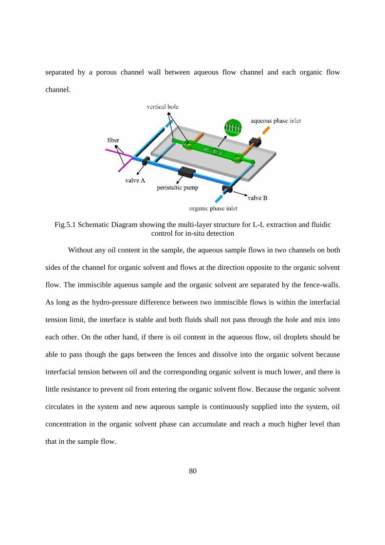
80

separated by a porous channel wall between aqueous flow channel and each organic flow

channel.

Fig.5.1 Schematic Diagram showing the multi-layer structure for L-L extraction and fluidiccontrol for in-situ detection

Without any oil content in the sample, the aqueous sample flows in two channels on both

sides of the channel for organic solvent and flows at the direction opposite to the organic solvent

flow. The immiscible aqueous sample and the organic solvent are separated by the fence-walls.

As long as the hydro-pressure difference between two immiscible flows is within the interfacial

tension limit, the interface is stable and both fluids shall not pass through the hole and mix into

each other. On the other hand, if there is oil content in the aqueous flow, oil droplets should be

able to pass though the gaps between the fences and dissolve into the organic solvent because

interfacial tension between oil and the corresponding organic solvent is much lower, and there is

little resistance to prevent oil from entering the organic solvent flow. Because the organic solvent

circulates in the system and new aqueous sample is continuously supplied into the system, oil

concentration in the organic solvent phase can accumulate and reach a much higher level than

that in the sample flow.

81

Fig.5.2 Schematic design diagrams of the top-view for the L-L extraction unit in counter-flowoperation

In comparison with the conventional static balance procedure, the organic solvent in this

design continuously circulates in the system and fresh aqueous sample is continuously supplied

to the system. The oil concentration of aqueous sample exiting is far from exacting balance, but

oil concentration in the organic solvent phase can accumulate, for any controlled time period,

until the maximum concentration is achieved, i.e., the equilibrium of the concentrations of oils in

the aqueous sample solution and organic phase is reached. For a portable device as targeted in

our design, the operation time shall be controlled in an acceptable period. The best approach is to

calibrate the relation between oil concentration of fresh aqueous sample and oil concentration of

organic solvent when the system operated for a given time period. Because the fenced walls

provide much higher diffusion efficiency in comparison with porous membrane and counter-

current flow (higher efficiency than that of the co-current design), the required operation time for

L-L extraction unit can be much shorter.

Organic flow Aqueous flowOil or organic solvent with oil

Peristalticpump

Valve AValve BPeristaltic pump

Aqueous sample reservoir

Organic solvent

To detection unit

82

After L-L extraction, the organic solvent with the extracted oil is then controlled by pump

and valves to flow through a microfluidic channel and enter the optical detection unit. The

detailed design and operation principle for the optical detection unit are shown in Chapter 3 and

Chapter 4. The optical measurement unit is integrated on the same chip as the microfluidic L-L

extraction unit, as well as microvalves and micropumps for flow control to form an integrated

micro-fluidic-optic cartridge. Optical fibers are used to supply and receive light from the

measurement chamber. Other optical components including light emitting diodes (LEDs) as

excitation light sources, spectrometer as detectors, and filters, are external components of the

instrument and not integrated with the micro-fluidic-optical cartridge. Because the fluorescence

characteristics of crude oil may vary depending on where the crude oil was from geographically,

this design allows different types of LEDs, detectors and filters to be chosen for the specific oil

sources and independently of the microfluidic chip.

For the L-L extraction layer, the depth of all channels is 600m. The aqueous phase

channel in the middle is 600μm wide. The organic phase channels on the two sides are 300m

wide each. The diameter of the vertical hole is 1mm. The length between two vertical holes is

3cm. The size of the fence wall will be discussed in later sections. The cross-sections of channels

in the electromagnetic control layer and the fluid handling layer are all 600m600m.

5.2.2 Counter-current and co-current flow configuration of the L-L extraction layer andinterface stability

There are two design options for L-L extractors. The first one is the so-called co-current

design in which the aqueous and the organic phases flow in the same direction. The second

design is the counter-current one in which the aqueous and organic phases flow in the opposite

83

directions as shown in Fig.5.3. Numerical simulations and experiments were used to compare the

extraction efficiencies of two designs.

For co-current flow design, the flow interface stability has been extensively studied,

especially for the conventional sized ones widely used in chemical industry. In micro-flow L-L

extractor, interfacial stability can be easily maintained with co-current design because the flow is

generally laminar. The main disadvantage of the co-current design is its lower extraction

efficiency because as the organic solvent flows out the system, the difference of the sample

concentration between the two flows drops significantly. As the result, there may be significant

amount of sample still left in the aqueous solution. In the counter-current flow design, a high

concentration gradient can be maintained as the organic phase flow from the downstream of the

aqueous phase and it is expected to obtain high solvent extraction.

Fig.5.3 Schematic diagrams of the liquid-liquid extractor in counter-current (a) and co-current (b)flows with physical separation

In theory, co-current fluids in micro flow channels are laminar. They will not mix into

each other even if no physical separation is used if the pressure differences in the flow channels

are carefully controlled. In reality however, some separation wall and surface modification are

obligatory for both designs. Numerical simulations were performed to study the extraction

efficiencies of both counter-current and co-current flows with a two-dimensional model. Fig.5.4

illustrates the distribution of concentration and mass flux of the solutes in both cases. As the

84

aqueous phase flows through the channel, the solute penetrates the fence wall and reaches the

organic phase because of the concentration difference. The result confirms that the concentration

decreases faster in the counter-current flow than that in the co-current flow along the channel. In

the co-current extractor, uniform concentration is immediately established so that the solute is

prevented from transferring between the two phases. On the contrary, a high concentration

difference is maintained during the extraction in the counter-current flow extractor, which drives

solute to move from the aqueous phase to the organic phase. Thus, higher extraction efficiency

can be eventually achieved.

Fig.5.4 Comparison of mass flux and concentration distribution of the solute in the extractor inco-current and counter-current flows

Fig.5.4 shows that comparison of mass flux and concentration distribution of the solute

in the extractor in counter-current flow and co-current flow. The extractor is 1.2mm in width and

2mm in height. The thickness of the porous wall is 0.2mm. The velocity of the organic phase and

aqueous phase is 0.6mm/s. Inlet concentration of solute is 1mol/m3. The diffusion coefficient is

1e-8 m2/s. The parameters of the model have been adjusted to show the difference between co-

current and counter-current flow more significant. These parameters used in numerical

simulations are in the same order of magnitude but not exactly the same sizes as used in our

85

design. The numerical simulation results show that the extraction efficiency of the counter-

current flow is always higher than co-current flow as expected.

The counter-current design is chosen for its high efficiency and because the fabrication

technology to be used provides us with the design flexibility. Two pressure values are

considered in the flow interface stability analysis. One is the pressure difference, Pflow between

two phases with different viscosity and velocity. The other is the Laplace pressure PLaplace

caused by the interfacial tension between the two phases. At very low Reynolds number (as in

microchannels), the pressure drop can be considered linear (Fig.5.5). The maximum Pflow is

located at the tips of the transfer region. When Pflow exceeds PLaplace, the interface cannot

sustain the pressure drop and break down.

Fig.5.5 Pressure profile of the two-phase flow along the channel

According to Young's law, the relationship between the contact angle and surface tension

is expressed as:

, (5-1)

where denotes contact angle. A is aqueous phase; O is the organic phase and S is the substrate

surface. , and are the surface tensions between the corresponding interfaces,

respectively. Additionally, the Laplace pressure across the interface in a pore can be evaluated as:

AO AS OS cos

AO

AS

OS

86

, (5-2)

where R is the curvature radius of the interface and d is the size of the pore. The major goal here

is to achieve higher PLaplace. Eq.5-1 indicates that the contact angle is submitted to the

characteristic of the substrate surface (i.e. and ), meanwhile PLaplace relies entirely on the

contact angle at a given flow condition. Ideally PLaplace reaches maximum at =0 or 180°. This

relationship implies that selective surface modification is a valid method to control the extraction

process. Much work has been devoted to this technique [68-70]. Arata etc [63] detailed a

theoretical model to analyze the pressure balance. A typical process is to form a hydrophilic-

hydrophobic pattern modification. The surface of the aqueous phase side is hydrophilic, while

that of the organic phase is hydrophobic (Fig.5.4). The range of the contact angle is between the

peak contact angle of organic phase org/philic and the hydrophilic surface and that of the aqueous

phase and the hydrophobic surface aq/phobic. On the basis of Eq.5-2, it can be written as:

. (5-3)

The selective surface modification provides wider range of PLaplace. It allows the

extractor operates at larger velocity difference between the two-phase flows. Consequently, the

extraction efficiency is improved.

Fig.5.6 (a) the shape of the interface when the organic phase moves to the hydrophilic surface;(b) the shape of the interface when the aqueous phase moves to the hydrophobic surface

PLaplace 2 AO R 4 AO Sin ( 90 0 ) d

OS

AS

4AOSin(org / philic 900) d PLaplace 4AOSin(aq / pholic 900) d

87

5.2.3 Material selection for L-L extraction layer: SU-8 or PDMS

The structure of L-L extraction layer is shown as green part in Fig.5.1 and dash part in

Fig.5.2. It is the most important layer in three layers of the L-L extraction system. Both the

electromagnetic control layer and the fluid-handling layer are fabricated with PDMS for ease of

fabrication. The L-L extraction system material can be selected between PDMS and SU-8. The

advantages and disadvantages of PDMS and SU-8 are compared.

a. Comparison of SU-8 and PDMS surface modification

In order to obtain high liquid-to-liquid extraction efficiency and two-phase counter flow

stability, large wettability difference on two opposite sides of the fence wall is highly desired.

The wall on the aqueous phase channel side is highly hydrophilic while the one on the organic

phase channel side is highly hydrophobic. To reach this goal, two different surface modification

techniques (hydrophilic on aqueous side and hydrophobic on organic side) on the same fence

wall are implemented.

Generally, Surface modification on SU-8 is easier than PDMS. Because of low adhesion

property of PDMS, it is always a problem to do surface modification on PDMS. For PDMS,

hydrophobic treatment is rare. But there are plenty of well-studied hydrophilic methods [71-74].

For a SU-8 substrate surface, both hydrophilic and hydrophobic surface treatments in

microfluidic channels are well known techniques.

The PDMS is hydrophobic naturally. Its contact angle of water is about 108. There are

some methods to improve its hydrophobic property. But they are either not significantly enough

or lasting very short. In fact, PDMS is naturally hydrophobic enough for our requirement. On the

other hand, some treatments can improve hydrophilic property of PDMS surface significantly.

Many techniques for hydrophilic treatments are reported, such as plasma treatment, UV

88

treatment, CVD, coating with metals and metal oxides, and many other wet chemical methods

[75]. The effective period is still a problem. Most of these treatments can only last several days

or several weeks. Our target is to make a commercial device. The shell life of the device should

last as long as possible. Therefore, a treatment of long life is chosen. It is reported that it can last

about two months. The details of the treatment are introduced in later section. Many types of

monomer can be deposited on the surface of PDMS, AA (anionic acrylic acid) is used in this

dissertation. Our experimental results show that the water contact angle can approach 40 after

using AA surface modification. ZW (zwitterionic [2-(methacryloyloxy)-ethyl] dimethyl (3-

sulfopropyl) ammonium) may be better and can be used in the future. Some research shows that

the water contact angle can be as low as 15 after using surface modified by ZW.

Cured SU-8 itself is relatively hydrophobic, with a water contact angle of 70-80 [76-

77]. To date, many hydrophilic surface modification techniques have been reported, including

oxygen plasma treatment, reaction with ethanolamine, or UV-initiated graft polymerization etc.

[71-72][74]. If only the surface of selected area (fence on the aqueous channel side only) needs

to be modified, UV initiated graft polymerization is proven to be more effective due to its ability

of micro-patterning surface with the aid of a mask [74]. UV-initiated graft polymerization of SU-

8 relies on the residual photoacid generator within the SU-8 matrix after being cured. With the

presence of a monomer solution and UV light, the remaining photoacid generator initiates the

polymerization of the monomer onto the SU-8 surface [78]. A wide range of water-soluble

monomers, such as poly(acrylic acid), poly(ethylene glycol) methyl ether acrylate and 2-

(dimethylamino) ethyl methacrylate, could be successfully photografted onto the surface of the

SU-8 photoresist surface. Two monomers candidates have been tested in our research: the first

89

one is poly(ethylene glycol) methyl ether acrylate with water contact angle 45°, and the other one

is 2-(dimethylamino) ethyl methacrylate with water contact angle 13°.

SU-8 can be made hydrophobic by coating with octadecyltrichlorosilane (OTS) [79-81].

After aqueous channel side of the fence have been hydrophilic modified, silanization (coated by

a covalent binding of octadecyltrichlorosilane (OTS) was then carried out on the organic phase

channel side. After the treatment, fence on the organic channel half (not covered by grafted

polymers) and the organic channels are silanized. A water contact angle of 110 can be achieved.

b. Comparison of SU-8 and PDMS fabrication

There are two design options for the fenced wall structures for L-L extraction separation,

one is the array of micro-posts, and the other is the porous fence. The fabrication of SU-8 porous

fence can be accomplished with multiple steps of normal lithography and tilting lithography

technique. The fabrication process of the wall with micro-pores to separate the input sample fluid

with the organic solvent is illustrated as following. The SU-8 layer is exposed twice, one at 45,

another at -45. An aligned normal exposure is then conducted to define the fluid channels

[27][82]. The size of the pores can be well controlled. Smaller these pores are, greater the surface

tension is. The flow rates of both phases are allowed to rise up. Since SU-8 is harder, the frame

can be thin and the total contact area between two phases can be larger. The extraction efficiency

would increase. The porous wall structure can only be achieved by SU-8.

However, the fabrication process of the porous wall is more complicated than that for the

fenced wall formed with array of the micro-posts.

The L-L extraction system consists of three functional layers: the electromagnetic control

layer, the fluid handling layer and the L-L extraction layer. The electromagnetic control layer

and the fluid handling layer were fabricated by PDMS. If the L-L extraction layer was fabricated

90

by SU-8, the rest two layers are bonded to the Su-8 layer in the top and bottom sides. If the L-L

extraction layer is fabricated with PDMS, the L-L extraction layer and the fluid handling layer

can be combined to be one layer. Both of them are fabricated in the same layer and then bond

with the electromagnetic control layer. As stated in section 5.2.3a, if it is made of PDMS, there is

only once surface modification needed. But if it is made of SU-8, it requires surface

modifications on both sides.

Bonding is another issue for SU-8. Bonding strength between PDMS and PDMS can be

achieved with oxygen plasma assisted method. Bonding strength between PDMS and SU-8

structures is a challenge. Direct oxygen plasma treatment has only resulted in a weak bonding

between PDMS and SU-8. Chueh et al., [83] proposed a leakage-free PDMS to polymer bonding

technique that used a thin layer of PDMS pre-polymer as a glue layer for the PDMS bonding to

various polymer surfaces. However the bonding strength is still weaker and the bonding process

is more complicated.

c. Summary of comparison

PDMS and SU-8 have their own advantages for the L-L extraction layer material. Firstly,

the surface modification of SU-8 can be easier than PDMS. For SU-8, the water contact angel

after hydrophilic treatment is 13 and hydrophobic is 110. For PDMS, the water contact angel

after hydrophilic treatment is 40 and hydrophobic is 108. The surface tension of the SU-8 is

greater, which means higher flow rate in the channel and more stability of the flow. The

hydrophilic on the PDMS can only last about two months; the hydrophilic and hydrophobic

treatment on SU-8 can last longer.

Secondly, with micro-molding process of, the separation wall between the aqueous phase

and organic phase can only be the fenced wall formed with array of micro-posts because the

91

walls with microholes cannot be molded. If SU-8 is used as the structural material for the device,

not the molded PDMS, then both the fenced wall formed with array of microposts and the wall

with micro porous can be used. The micro porous wall may improve extraction efficiency

significantly.

However, the molding fabrication process of PDMS is simpler and may reduce the

overall cost of the device significantly. The L-L extraction layer and the fluid handling layer can

be combined as one layer. On the other hand, bonding strength between PDMS and PDMS is

better than PDMS and SU-8.

Both of PDMS and SU-8 have their advantages and disadvantages respectively for L-L

extraction layer material. PDMS is chosen in this dissertation, but SU-8 is still a potential option

for future work.

5.2.4 Surface modification of the PDMS L-L extraction layer

The following procedure was used for surface modification of the PDMS samples: 1) to

immerse PDMS sample in acetone solution containing 10wt% benzophenone (Sigma Aldrich)

for 40s, and then blow it dry with nitrogen. Benzophenone can be excited photochemically with

UV irradiation. The purpose of immersing PDMS in it is to diffuse some benzophenone into the

PDMS surface and to use it as a photoinitiator in the UV-induced reaction later; 2) Prepare a

solution with 5 wt% in water monomer, 0.5 mM NaIO4 (Sigma Aldrich), and 0.5 wt% benzyl

alcohol (Sigma Aldrich); 3) Coat the solution on the PDMS; 4) Prepare a UV-transparent glass

slide and clean it up in a 5: 1 mixture of Milli-Q water and 35wt% hydrogen peroxide for 10 min

at 80C; 5) Load the glass slide carefully onto the PDMS to contact the solution coated on the

PDMS sample. After completely contact with the solution, the PDMS is adhered below the glass

because of the surface tension as shown in Fig.5.7; 6) UV exposure.

92

The temperature needs be controlled in this process. If the temperature rose up because of

the UV exposure in later processing step, a phase transition may happen and polymer chain may

aggregate. To control the temperature, a frame is made to support the PDMS so that the lower

surface of the substrate is maintained to contact ice water in the dish. Finally the sample was

placed under the UV lamp for exposure. The UV intensity was about 8 mW /cm2. The Exposure

took about 40 min. After the exposure, the PDMS sample was removed from the glass slide and

washed with deionized water and ethanol for 15mins, then incubated in deionized water

overnight to eliminate the loosely deposited but not covalently attached monomer and polymer

from the PDMS surface.

There are a few options for the monomer, such as cationic dimethylacrylamide (DMAA),

anionic acrylic acid (AA), and zwitterionic [2-(methacryloyloxy)-ethyl] dimethyl (3-sulfopropyl)

ammonium (ZW). AA is used in this dissertation. Some studies show that the water contact angle

can approach 40 after using AA surface modification. Some research shows that the water

contact angle can be as low as 15 after using surface modified by ZW [84]. ZW may be better

and can be used in future work.

Fig.5.7 Schematic diagram of the PDMS surface modification

93

5.2.5 Fabrication of L-L extraction layer

The design of L-L extraction layer is shown in Fig.5.1, and its operation principle has

been introduced. The schematic diagram of fabrication procedure for the L-L extraction layer is

shown in Fig.5.8. Step 1 was to fabricate the SU-8 mold. The thickness of the SU-8 was 600μm.

The side length of the vertical rectangle holes was variable and can be well controlled. In Step 2,

a negative PDMS pattern was created using a soft lithograph process. In Step 3, the cast-molded

PDMS structure was carefully peeled off the SU-8 master mold. Because the micro-posts were

thin and fragile, the peeling process needs to be carried out carefully and from one side to the

other. The micro-posts need to be peeled off the master mold one by one. After peeling off, the

sample was placed on a clean wafer. In step 4, SU-8 photoresist was poured onto the PDMS and

excessive SU-8 was scraped off with a clean razor blade and then placed in a vacuum chamber

for 20 minutes to eliminate air bubbles. Low viscosity SU-8 was better for filling in to the

microstructures and quickly eliminating air bubbles. SU-8 50 was used in this research. After

Step 4, the following was standard SU-8 lithography process, prebake, exposing, post bake and

developing. It is worth noting that the photomask was aligned onto the PDMS substrate and SU-

8 after prebake by using Quintel UL7000-OBS Aligner and DUV Exposure Station. The SU-8

was exposed on selected area as shown in Step 5. After development, only selected area

remained as in Step 6. Step 7 was used to carry out the surface modification for the PMDS

sample. Because the coated SU-8 layer protected the selected regions, only the unprotected

regions were surface modified. The detail surface modification process was introduced in section

5.2.4. After the surface modification, the SU-8 protective layer was removed. Thanks to the low

adhesion property of PDMS, SU-8 protective layer could be easily removed mechanically with

94

the help of a needle. In Step 8 the top of the L-L extraction channel was sealed with a layer of

PMDS membrane. This completed the fabrication of the L-L extraction channel.

Limited by the molding process, the sizes of the rectangle micro-posts of the fence wall

cannot be too small. In Step 1, the rectangle holes were not through holes. Thus, it was difficult

to completely clean the bottoms of the holes by developer if the sizes of these holes are too small,

and would negatively affect the following processing steps. Especially after PMDS molding, the

PDMS micro-posts might become shorter than the sidewalls, and therefore could not be bonded

to the top membrane when the entire micro-fluidic-optic chip was integrated in bonding process.

Even if they were bonded together, there would be gaps between micro-posts and the top

membrane, and if the gaps were big enough, the aqueous and organic phase solutions might

easily flow through them with little pressure. If the size of the micro-holes made on SU-8 was

too small in Step 1, the molding process with PDMS might become impossible because the

molded PDMS micro-posts might be too small and fragile, and could be easily broken during the

peeling off process in Step3. After many experiments, it was proved the size of the rectangle

poles must be bigger than 150μm150μm.

95

Fig.5.8 Schematic diagram of the fabrication process for the L-L extraction layer

Sealing the top

96

5.2.6 Simulation of L-L extraction layer extraction efficiency

A numerical simulation was performed to study the extraction efficiency of the L-L

extraction layer in counter flow with a 2-dimensional model. Similar simulations were reported

by other researchers [85]. The only difference in our mold is the fence wall structure. The model

was built and the fluid in the fence wall was considered as static layer of fluid. For the entire

organic phase channel that forms a loop, cross-section area is 600μm600μm. The flow rate of

the peristaltic pump is 3l/min. The total length of the looped channel for the organic phase is

about 8cm. Therefore, the total time for organic phase flowing one circle is therefore calculated

to be 9.6 mins.

The L-L extraction layer is symmetric, thus we can simulate half of it. As shown in

Fig.5.3a, we can assume the oil concentration of aqueous phase on the entrance is C0 and the oil

concentration of organic phase on the exit is C. In theory, if the thickness of the fence wall is

smaller, the extraction efficiency is better, because the traveling distance for oil is shorter as it

diffuses from the aqueous phase to organic phase. Limited by the fabrication process, the

achievable minimum size of the poles’ cross-section was found to be 150m150m. The cross-

section of the micro-posts was set to be 150m150m in simulation and the gaps between the

poles were also set to be 150m. The flow rate of the aqueous phase was set as 150μl/min.

Fig.5.9 shows the simulated results of C/C0 as a function of time. For the first circle, C/C0

has an equilibrium state as shown in Fig.5.9a. After 3 minutes, C/C0 reached over 90% value of

the equilibrium state. To simplify the simulation of the system, assume that there is no diffusion

after the organic fluid leaving the L-L extraction layer. It means when it leaves the exit of the L-

L extraction layer, the oil concentration distribution of the organic phase is the same as it enters

the entrance in the next round of circular flow. From this assumption, the relation between C/C0

97

and time of the second circle is shown in Fig.5.9b. C/C0 also has an equilibrium state. After

about 14 minutes of virtual operation, C/C0 has reached over 90% valve of the equilibrium state.

Fig.5.9 The relation between C/C0 and time in the first (a) and second (b) flow circle

Fig.5.10 Oil concentration distribution of both organic and aqueous phase in the first and secondflow circle

Fig.5.10 illustrates the equilibrium state distribution of concentration and mass flux of the

solute in the first and second circle. As the length of both phases is 3cm while the width is only

300m, the length is 20 times smaller in the figure to give a better view. Figs. 5.10a and b are the

oil concentration distribution of the organic phase and aqueous phase in the first circle; Fig.

5.10c and 5.10d are the oil concentration distribution of the organic phase and aqueous phase in

98

the second circle respectively. The simulation results show that the oil concentration magnitude

of the organic phase after 15mins extraction operation can be as high as 7 times of concentration

in aqueous sample without extraction.

5.3 Experimental results of the integrated system and comparison of different fence sizedesigns

The design of the integrated micro-fluidic-optic chip was shown in Section 5.1. The

optical detection unit was designed and presented in Chapter 3. The peristaltic pump was

designed and discussed in Chapter 4. The size of the micro-posts forming the fence wall as the

physical separation between the organic phase and aqueous sample solutions in the L-L

extraction layer and the gaps between the poles need to be studied. In theory, the smaller the size

of the micro-posts is, the higher the extraction efficiency can be because the thickness of the

fence wall is thinner and it is easier for oil passing through. Several different sizes of microposts

were tried to prove this theory. As discussed in Section 5.2.5, limited by the fabrication process,

the minimum cross-section of the micro-posts’ is 150m150m. In this dissertation

150m150m600m, 200m200m600m and 250m250m 600m poles were tried.

To keep the contact area between organic and aqueous phases the same for different designs of

the micro-posts, the gaps between the poles were set to be 150m, 200m and 250m

respectively.

The organic phase was driven to circulate in the micro-channel by a specially constructed

peristaltic pump. As mentioned in Chapter 4, with a step time of 0.1s, the flow rate of the

peristaltic pump was found to be about 3μl/min under free load condition. When the integrated

micro-fluidic-optic chip operates, the flow resistance of the organic phase must be greater than

free load. Thus, the flow rate of the peristaltic pump may be slightly lower than 3μl/min. The

99

aqueous phase was designed to be driven with an external pump. In our experiments, it was

driven by the syringe pump (NE-4002X Syringe pump), which can control the flow rate

accurately.

The surface tension is an inherent physical property of a fluid. For the aqueous, and the

organic phase fluid, how hard for these two fluids to flow across the fenced wall formed by the

array of micro-posts depends heavily on the gaps between the neighboring micro-posts. When

the gaps are smaller, higher pressure difference is required to drive the fluids to flow to the

opposite sides of the fence wall. This means that the flow rate of the organic phase can be higher

with no concern for leakage to the opposite side of the fence wall.

In our experiment, while the peristaltic pump continues to operate, the aqueous phase

sample was supplied into the system with an external syringe pump. The aqueous and the organic

phase solutions flow in counter-directions. The flow rate of the aqueous phase was gradually

increased to find the maximum flow rate while the stable interfacial surface still maintained. The

maximum flow rate of the aqueous phase flow rate was measured for different sizes of micro-

posts in the fence wall. If the flow rate of the input aqueous solution was higher than the

maximum rate permitted, the interface between the two phases would be broken through and two

phases would mix together.

The maximum aqueous phase flow rate was measured for three different designs of fence

wall formed with the micro-posts and gaps. The result was that the maximum of the aqueous

phase flow rate of for the fence wall of 150m150m600m micro-posts and 150m gaps

design was about 150l/min. The maximum of the flow rate for the fence wall of

200m200m600m micro-posts and 200m gaps was about 50l/min. And for fence wall

100

with 250m250m600m micro-posts and 250m gaps, the interface was not stable at any

aqueous phase flow rate.

We have conducted some experiments to test the integrated system using fence walls

with the two different designs of the micro-post and gap sizes using standard oil samples. Crude

oil was provided by BP Company. The samples with 1ppm, 50ppm concentrations were prepared

with nonane as solution. A commercial spectrometer was used to measure the output spectrum of

the photodiode signal. The integration time of the signal (amplitude) in the spectrometer was

adjusted correspondingly. The extraction time was set to be 15 minutes. The flow rate of the

aqueous phase was set to be close to maximum. Fig.5.11 shows the experimental results.

Fig.5.11a shows the output signal obtained by the spectrometer for the 1ppm concentration

sample without using the L-L extraction unit. Without extraction, the sample with 1ppm oil

concentration was undetectable. The same sample of 1ppm oil concentration was also used

experiments shown in Figs.5.11b, c, and d respectively. In Fig.5.11b and c, fence wall in the L-L

extractor was formed by array of micro-posts with cross-sectional area of 200μm200μm with

height of 600μm and 200μm gaps. In the experimental results shown in Fig. 5.11b, counter flow

scheme was used, i.e., the aqueous and organic phase solutions were flowing in opposite

directions. Fig.5.11c shows the results obtained with the aqueous and organic phase solutions in

co-current flow. The result shows that the sample with 1ppm oil concentration is detectable after

L-L extraction unit was used. However, the difference between counter flow and current flow is

not significant. This observation is different from the results obtained in numerical simulations

and analysis. In experiment shown in Fig.5.11d, the fence wall consists of array of micro-posts

with sizes of 150μm150μm and height of 600μm and gaps of 150μm was used in counter-flow

scheme. The resulting signal is greater than in Figs.5.11c and d.

101

Fig.5.11 Experimental results of the integrated system a) 1ppm sample without L-L extraction; b)1ppm sample with fence wall of 200μm by 200μm micro-posts and gaps and counter flow L-Lextraction; c) 1ppm sample with fence wall of 200μm by 200μm micro-posts and gaps and co-

current flow L-L extraction; d) 1ppm sample with fence wall with 150μm by 150μm micro-postsand 150μm gaps in counter flow extraction

Fig.5.12 shows another group of experimental results. Fig.5.12a shows the experimental

results of the standard sample of 50ppm oil concentration with no L-L extraction. Samples with

oil concentration of 50ppm were also used in experiments shown in Figs.5.12b, c and d. In

Fig.5.12b and c, fence wall formed with micro-posts of 200μm200μm cross-section and height

of 600μm and gaps of 200μm was used in the L-L extraction unit. In Fig.5.12b, counter-current

flow scheme was used in experiments shown in Fig.5.12b, and co-current flow scheme was used

in the experiments shown in Fig.5.12c. The difference in results between counter-current flow

and co-current flow was still not significant. In the experiment shown in Fig.5.12d, fence wall

formed with array of micro-posts of 150μm150μm cross-section, height of 600μm and gaps of

150μm was used in the L-L extraction unit. The aqueous and organic phase flows were

controlled in counter-current flows. The two significant fluorescent peaks of the oil are clearly

observed in Figs.5.12b c and d. The peak of 480nm is far away from the excitation light

wavelength and in theory least affected by it. The value of 480nm peak is taken to count the

magnification of extraction comparing with the results obtained without using L-L extraction. In

102

Fig.5.12b and c, the magnification ratios are close to 2 times, and in Fig.5.12d it is about 7 times.

The experimental results agree well with the predictions from numerical simulations.

Fig.5.12 Experimental results of the integrated micro-fluidic-optic chip: a) experimental resultsof sample with 50ppm oil concentration without extraction; b) experimental results of sample

with 50ppm oil concentration and counter flow extraction using fence wall formed with micro-posts with cross-sectional area of 200μm by 200μm and gaps of 200μm; c) experimental resultsof sample with 50ppm oil concentration using fence wall formed with micro-posts with cross-

sectional area of 200μm by 200μm and gaps of 200μm and co-current flow extraction; d)experimental results of sample with 50ppm oil concentration, fence wall formed of micro-posts

with cross-sectional area of 150μm by 150μm and gaps of 150μm, counter-current flowextraction

These experimental results have proved that the L-L extraction is useful and the

sensitivity of the device is significantly increased. The measurement sensitivity of the instrument

was improved to be better than 1ppm. It was also found that the optimal design for the separation

fence wall is the design with a cross-sectional area of 150μm150μm, the height of 600μm, and

gaps of 150μm between the neighboring posts. The reason is that the static fluid in the gaps is

shorter for the oil passing through, the extraction between two flowing phase should be faster.

And the aqueous phase flow rate is faster in the design with the array of micro-posts of

150μm150μm with height of 600μm and gaps of 150μm, the quantity of emulsified oil passed

through the channel is much more, therefore the accumulation of oil in organic phase is faster.

No significant difference is observed between the results for the counter-current and co-current

flows. The main reason may be that the flow rate of the peristaltic pump is very low, only at

3μl/min under free load. The flow rate might have become even lower in our experiments with

103

load while the flow rate of the aqueous phase is much greater. Thus, the flow rate of the organic

phase is so low that there is not much difference between the counter flow and co-current flow.

5.4 Conclusions

In this chapter, design and principle of the Liquid-to-Liquid extraction unit has been

introduced. The liquid-to-liquid extraction consists of three layers. Both cured SU-8 polymer and

PDMS are used in fabrication of the L-L unit. Both materials have their own advantages and

disadvantage. The L-L extraction unit presented in this dissertation has been built using PDMS

as the main material. SU-8 can be taken as another option in future depends on the specific

applications. The separation fence wall surface of the L-L extraction unit was selectively

modified to stabilize the two liquid phases in the microfluidics system. The detail technology and

processes of the surface modification process have also been presented. The experimental results

show that the hydrophobic and hydrophilic properties of the selected surfaces of the fence walls

have been significantly improved.

The numerical simulation results of the extraction efficiencies of two fluid phases have

proved that the counter-current flow scheme is better than that of the co-current flow one.

Prototypes of the micro-fluidic-optic chips have been fabricated. The optical detection system,

the peristaltic micropump and the liquid-to-liquid (L-L) extraction microfluidic system were

integrated together. Experiments were conducted to test the prototypes of the microchips. The

experimental results have shown that the L-L extraction layer function very well and the

sensitivity of the entire system have been enhanced in comparison with those without L-L

extraction as shown in Chapter 3. The resolution of the entire system has been improved to blow

1ppm. The study has also found that the optimal design for the fence wall is to use array of

micro-posts with cross-sectional area of 150μm150μm and height of 600μm, with the gaps

104

between the neighboring posts to be 150μm. The experimental results have shown that the

sensitivity has been improved as high as 7 times after 15mins extraction. The experimental

results agree well with the predictions of numerical simulations. The experimental results have

also shown that no significant difference was observed between the results by using co-current

flow and the counter-current flow schemes, in contrary to what has been expected based on

theoretical analysis. The main reason for is may be that the flow rate of the organic phase is too

low, which made the difference of the flow velocities of the organic phase and the aqueous phase

flows are negligible. To overcome this problem, better micro-pumps should be designed and

built to increase the flow rate, and therefore to increase the flow velocity of the organic phase

solution. Therefore, to improve the flow rate of the micropump is one of future research tasks.

In conclusion, our study has proved the feasibility of the design and fabrication of an

integrated micro-fluidic chip based instrument for in-situ detection of spilled oil in water. Further

work is still needed to improve the sensitivity of the system.

105

CHAPTER 6 CONCLUSIONS

A new generation of instruments for spilled oil detection is highly desired for

applications for in-situ measurements. Specifically, the new generation of instruments should

meet the following requirements: 1) In-situ sensors should be the priority; 2) with the lower

detection limit in 0.1 – 1 ppm and upper detection limit at least 100 ppm; 3) easily deployable

and portable; 4) simplicity of use, be simpler to use than Turner, that is, be easier to set up and

standardize; 5) Reliability – Turner setup may vary from day to day and is sensitive to rough

handling. New instrument must be robust; 6) Easier Logistics – New system must have fewer

components and must be lighter and require less logistics than the current system that requires

two large boxes weighing 75-100 lbs each; 7) require less maintenance and lower maintenance

costs; 8) Must be capable of being integrated with Windows operating systems and GPS. From

the experiment results of the integrated system, these requirements are meted.

The research work presented in this dissertation targeted to develop a new generation of

spilled oil detection instruments to meet these requirements. The key point in miniaturizing the

physical sizes while still maintaining the sensitivity of sensors is to miniaturize the extraction

processing and also to integrate the extraction and detection on the same chip substrate. Only the

monitoring and displaying unit, the power supply, and other parts need to be external. All the

external parts are well selected. Multiple designs of the micro-optic detection systems were

tested and compared, and an optimal design was then selected. The output signal without

extraction was calibrated by standard density samples. The detection limit without extraction was

found to be between 1ppm and 10ppm.

An out-of-plane lens was designed and fabricated to enhance the sensitivity of the optical

detection unit. The fabrication process and the property of the lens were studied both

106

theoretically and experimentally, and eventually a lens design with one-membrane was and

selected and constructed to integrate with the optical fiber.

Both the co-current and counter-current designs of the liquid-liquid extraction system

were studied and compared. A peristaltic pump was designed, built, and used to deliver the flow

for the micro-fluidic chip. The pump was controlled using a Labview program. The controlling

program can be integrated with any operating systems. Different designs of the pumps were also

tested and compared. The maximum flow rate of the prototype micropump was found to be about

3μl/min. The experimental results showed that the best design of the L-L extraction unit can

increase the oil density in the organic phase solution by as much as 7 times of the oil density in

the aqueous phase. Therefore the detection limit is improved by 7 times. The final oil detection

resolution was found to be lower than 1ppm. Besides the computer and the monitor, the rest part

of the device can be controlled under 10cm10cm10cm cubic and the weight can be less than 5

lbs.

107

REFERENCES

1. Lisa P. Jackson (May 24, 2010), Statement by EPA Administrator Lisa P. Jackson from PressConference on Dispersant Use in the Gulf of Mexico with U.S. Coast Guard Rear AdmiralLandry, Environmental Protection Agency.

2. Richard A. Kerr (13 August 2010). "A Lot of Oil on the Loose, Not So Much to BeFound". Science 329 (5993): 734–5. DOI:10.1126/science.329.5993.734.PMID 20705818

3. Fingas, Merv. The basics of oil spill cleanup. CRC, 2000.

4. Kingston, P. F. (2002). Long-term Environmental Impact of Oil Spills. Spill Science &Technology Bulletin, 7(1-2), 53-61. doi:10.1016/S1353-2561(02)00051-8

5. Wolfe, D. A. "eleven coauthors. 1994. The fate of the oil spilled from the ExxonValdez." Environmental Science and Technology 28: 561.

6. Short, Jeffrey W., et al. "JJ &. Rice, SD (2004). Estimate of oil persisting on the beaches ofPrince William Sound 12 years after the Exxon Valdez oil spill."Environmental Science andTechnology: 19-25.

7. Murphy, Michael L., et al. "Recovery of pink salmon spawning areas after the Exxon Valdezoil spill." Transactions of the American Fisheries Society 128.5 (1999): 909-918.

8. Bue, Brian G., Samuel Sharr, and James E. Seeb. "Evidence of damage to pink salmonpopulations inhabiting Prince William Sound, Alaska, two generations after the Exxon Valdezoil spill." Transactions of the American Fisheries Society 127.1 (1998): 35-43.

9. Peterson, C. H., Rice, S. D., Short, J. W., Esler, D., Bodkin, J. L., Ballachey, B. E., & Irons, D.B. (2003). Long-term ecosystem response to the Exxon Valdez oil spill. Science (New York,N.Y.), 302(5653), 2082-6. doi:10.1126/science.1084282

10. Teal, J. M., & Howarth, R. W. (1984). Oil spill studies: A review of ecological effects.Environmental Management, 8(1), 27-43. doi:10.1007/BF01867871

11. Wang, Z., Fingas, M., & Page, D. S. (1999). Oil spill identification. Journal of ChromatographyA, 843(1-2), 369-411. doi:10.1016/S0021-9673(99)00120-X

12. Kasap, S. O. "Photovoltaic devices." Optoelectronics and photonics: Principles andpractices (2001): 254-272.

13. Joint Analysis Group (May 2010), Review of R/V Brooks McCall Data to Examine Surface Oil.

14. SL Ross Environmental Research “Updating the Smart Dispersant Monitoring Protocol:Review of Commercial-Off-The-Shelf Instruments Final Report”, Ottawa, ON, August, 2008.

108

15. Tanaka, M. (2007). An industrial and applied review of new MEMS devices features.Microelectronic Engineering, 84(5-8), 1341-1344. doi:10.1016/j.mee.2007.01.232

16. C.T.-C. Nguyen, IEEE Transactions on Microwave Theory and Techniques 47 (August) (1999)1486–1503.

17. Zengxuan Cai, Qun Fang, et al. (2006), A Microfluidic Chip Based Liquid-Liquid ExtractionSystem With Microporous Membrane, Anal. Chem. Acta., p 151-156.

18. Xiaoyan Wang, Chutarat Saridara and Somenath Mitra (2005), Microfluidic Supported LiquidMembrane Extraction, Anal. Chem. Acta. , p 92-98.

19. Jason G. Kralj, Hemantkumar R. Sahoo and Klavs F. Jensen (2007), Integrated ContinuousMicrofluidic Liquid-Liquid Extraction, Lab chip, p 256-263.

20. Jeong, Ok Chan, et al. "Fabrication of a peristaltic PDMS micropump." Sensors and ActuatorsA: Physical 123 (2005): 453-458.

21. Husband, Ben, et al. "Investigation for the operation of an integrated peristalticmicropump." Journal of Micromechanics and Microengineering 14.9 (2004): S64.

22. Jang, Ling-Sheng, et al. "A stand-alone peristaltic micropump based on piezoelectricactuation." Biomedical microdevices 9.2 (2007): 185-194.

23. Nussbaum, Ph, et al. "Design, fabrication and testing of microlens arrays for sensors andmicrosystems." Pure and Applied Optics: Journal of the European Optical Society Part A 6.6(1999): 617.

24. Chen, Jackie, et al. "Variable-focusing microlens with microfluidic chip." Journal ofMicromechanics and Microengineering 14.5 (2004): 675.

25. Chan, Edwin P., and Alfred J. Crosby. "Fabricating microlens arrays by surfacewrinkling." Advanced Materials 18.24 (2006): 3238-3242.

26. R. Yang and W. Wang, "A numerical and experimental study on gap compensation andwavelength selection in UV-lithography of ultra-high aspect ratio SU-8 microstructures,"Sensors and Actuators B: Chemical 110(2), 279-288 (2005)

27. R. Yang and W. Wang, "Out-of-plane polymer refractive microlens fabricated based on directlithography of SU-8," Sensors and Actuators A: Physical 113(1), 71-77 (2004)

28. W. Dai, K. Lian, and W. Wang, "Design and fabrication of a SU-8 based electrostaticmicroactuator," Microsystem Technologies 13(3), 271-277 (2007)

109

29. Schulz, Craig M., and Jaromir Ruzicka. "Real-time determination of glucose consumption bylive cells using a lab-on-valve system with an integrated microbioreactor." Analyst 127.10(2002): 1293-1298.

30. Erxleben, Holger A., et al. "A novel approach for monitoring extracellular acidification rates:based on bead injection spectrophotometry and the lab-on-valve system." Analyst 129.3 (2004):205-212.

31. Shackman, Jonathan G., et al. "Perfusion and chemical monitoring of living cells on amicrofluidic chip." Lab on a Chip 5.1 (2005): 56-63.

32. Roman, Gregory T., et al. "Single-cell manipulation and analysis using microfluidicdevices." Analytical and bioanalytical chemistry 387.1 (2007): 9-12.

33. Davidsson, Richard, et al. "Microfluidic biosensing systems." Lab Chip 4.5 (2004): 488-494.

34. Tani, Hirofumi, Koji Maehana, and Tamio Kamidate. "Chip-based bioassay using bacterialsensor strains immobilized in three-dimensional microfluidic network." Analyticalchemistry 76.22 (2004): 6693-6697.

35. Jing-Lin Fu, Qun Fang et al. (2006), Laser-Induced Fluorescence Detection System forMicrofluidic Chips Based on an Orthogonal Optical Arrangement, Anal. Chem. 78, p 3827-3834.

36. Gwo-Bin Lee, Che-Hsin Lin and Shen-Chie Chang (2005), Micromachine-based Multi-channelFlow Cytometer for Cell/Particle Counting and Sorting, J. Micromech and Microeng., 15, p447-454

37. Rajinder Pal (1994), Techniques for Measuring the Composition (Oil and Water Content) ofEmulsions-a State of the Art Review, Colloids and Surfaces A, 84, p 141-193.

38. Lawrence R. Morrow, Wilson K. and Martir, Hossein Aghazeynali (1995), FluorescenceMethod of Quantifying Hydrocarbons, Including Crude Oil, Dispersed in Water. US Patent5,381,002.

39. Woias, Peter. "Micropumps—past, progress and future prospects." Sensors and Actuators B:Chemical 105.1 (2005): 28-38.

40. Jeffrey Y. Pan,Pinyen Lin, Fariborz Maseeh and Stephen D. Senturia(1990), Verification ofFEM analysis of load-deflection methods for measuring mechanical properties of thin films,Solid-State Sensor and Actuator Workshop, 1990. 4th Technical Digest., IEEE

41. N. Chronis, G. Liu, K.-H. Jeong, and L. Lee, "Tunable liquid-filled microlens array integratedwith microfluidic network," Opt. Express 11(19), 2370-2378 (2003)

110

42. Reyes, Darwin R., et al. "Micro total analysis systems. 1. Introduction, theory, andtechnology." ANALYTICAL CHEMISTRY-WASHINGTON DC- 74.12 (2002): 2623-2636.

43. Auroux, Pierre-Alain, et al. "Micro total analysis systems. 2.Analytical standard operations andapplications." ANALYTICAL CHEMISTRY-WASHINGTON DC- 74.12 (2002): 2637-2652.

44. Maillefer, Disier, et al. "A high-performance silicon micropump for an implantable drugdelivery system." Micro Electro Mechanical Systems, 1999. MEMS'99. Twelfth IEEEInternational Conference on. IEEE, 1999.

45. Zhang, Tao, and Qing-Ming Wang. "Valveless piezoelectric micropump for fuel delivery indirect methanol fuel cell (DMFC) devices." Journal of Power Sources140.1 (2005): 72-80.

46. Diaz J, Lopera JM, Pernia AM (2007) A micropump for pulmonary blood flow regulation. IndElectron Mag IEEE 1:39–44.

47. Amirouche, F., Zhou, Y., & Johnson, T. (2009). Current micropump technologies and theirbiomedical applications. Microsystem Technologies, 15(5), 647–666.

48. Nguyen, Nam-Trung, et al. "Integrated flow sensor for in situ measurement and control ofacoustic streaming in flexural plate wave micropumps." Sensors and Actuators A: Physical 79.2(2000): 115-121.

49. Wallman, Lars, et al. "Autonomous protein sample processing on‐ chip using solid‐ phasemicroextraction, capillary force pumping, and microdispensing."Electrophoresis 25.21‐ 22(2004): 3778-3787.

50. Suzuki, Hiroaki, and Rei Yoneyama. "Integrated microfluidic system with electrochemicallyactuated on-chip pumps and valves." Sensors and Actuators B: Chemical 96.1 (2003): 38-45.

51. Ehwald, Rudolf, et al. "Method for control of the volume flux of a liquid in an osmoticmicropump and osmotic micropump." U.S. Patent No. 7,976,535. 12 Jul. 2011.

52. Kilani, Mohammad I., et al. "Design and analysis of a surface micromachined spiral-channelviscous pump." Journal of fluids engineering 125.2 (2003): 339-344.

53. Terray, Alex, John Oakey, and David WM Marr. "Microfluidic control using colloidaldevices." Science 296.5574 (2002): 1841-1844.

54. Xie, Jun, Jason Shih, and Yu-Chong Tai. "Integrated parylene electrostatic peristalticpump." Proceedings of Micro TAS (2003): 865-868.

55. Kim, Ki Hoon, et al. "Fabrication and test of a micro electromagnetic actuator."Sensors andActuators A: Physical 117.1 (2005): 8-16.

111

56. Goldschmidtböing, F., et al. "A generic analytical model for micro-diaphragm pumps withactive valves." Journal of Micromechanics and Microengineering15.4 (2005): 673.

57. Jeong, Ok Chan, and Satoshi Konishi. "Fabrication of a peristaltic micro pump with novelcascaded actuators." Journal of Micromechanics and Microengineering 18.2 (2008): 025022.

58. Hulme, S. Elizabeth, Sergey S. Shevkoplyas, and George M. Whitesides. "Incorporation ofprefabricated screw, pneumatic, and solenoid valves into microfluidic devices." Lab Chip 9.1(2008): 79-86.

59. Manual on Disposal of Refining Wastes. American Petroleum Institute (1969), p 5-15.

60. Zengxuan Cai, Qun Fang, et al. (2006), A Microfluidic Chip Based Liquid-Liquid ExtractionSystem With Microporous Membrane, Anal. Chem. Acta., p 151-156.

61. Xiaoyan Wang, Chutarat Saridara and Somenath Mitra (2005), Microfluidic Supported LiquidMembrane Extraction, Anal. Chem. Acta. , p 92-98.

62. Jason G. Kralj, Hemantkumar R. Sahoo and Klavs F. Jensen (2007), Integrated ContinuousMicrofluidic Liquid-Liquid Extraction, Lab chip, p 256-263.

63. Arata Aota, Masaki Nonoka, et al. (2007), Countercurrent Laminar Microflow for HighlyEfficient Solvent Extract, Angew. Chem. Int. Ed., 46, p 878-880.

64. Manabu Tokeshi, Tomoko Minagawa, et al. (2002), Continuous-Flow Chemical Processing ona Microchip by Combining Microunit Operations and a Multiphase Flow Network, Anal.Chem., 74, p 1565-1571.

65. Akihide Hibara, Masaki Nonaka, et al. (2002), Stabilization of Liquid Interface and Control ofTwo-Phase Confluence and Separation in Glass Microchips by Utilizing OcatadecylsilaneModification of Microchannels, Anal. Chem., 74, p 1724-1728.

66. Arata Aota, Akihide Hibara and Takehiko Kitamori (2007), Pressure Balance at the Liquid-Liquid Interface of Micro Countercurrent Flows in Microchips, Anal. Chem., 79, p 3919-3924.

67. Ryan T. Kelly, Jason S. Page, et al. (2009), Dilution-free Analysis from Picoliter Droplets byNano-Electrospray Ionization Mass Spectrometry, Angew. Chem. Int. Ed., 48, p 6832-6835.

68. B. Zhao, J. S. Moore, D. J. Beebe (2001), Surface-Directed Liquid Flow inside Microchannels,Science, 291, 1023-1026.

69. A. Hibara, S. Iwayama, S. Matsuoka, et al. (2005), Surface Modification Method ofMicrochannels for Gas−Liquid Two-Phase Flow in Microchips, Anal. Chem. 77, 943-947.

112

70. A. Hibara, M. Nonaka, et al. (2003), Spectroscopic Analysis of Liquid/Liquid Interfaces inMultiphase Microflow, J. Am. Chem. Soc.,125, 14954-14955.

71. Tseng, Fan-Gang, et al. "A surface-tension-driven fluidic network for precise enzyme batch-dispensing and glucose detection." Sensors and Actuators A: Physical 111.1 (2004): 107-117.

72. Nordström, Maria, et al. "Rendering SU-8 hydrophilic to facilitate use in micro channelfabrication." Journal of Micromechanics and Microengineering 14.12 (2004): 1614.

73. Dai, Wen, and Wanjun Wang. "Selective metallization of cured SU-8 microstructures usingelectroless plating method." Sensors and Actuators A: Physical 135.1 (2007): 300-307.

74. Wang, Yanting, and Gregory A. Voth. "Unique spatial heterogeneity in ionic liquids." Journalof the American Chemical Society 127.35 (2005): 12192-12193.

75. Zhou, J., Ellis, A. V., & Voelcker, N. H. (2010). Recent developments in PDMS surfacemodification for microfluidic devices. Electrophoresis, 31(1), 2–16.doi:10.1002/elps.200900475

76. Yuli Wang et al. (2006), Simple Photografting Method to Chemically Modify and Micropatternthe Surface of SU-8 Photoresist, Langmuir, 22, 2719-2725.

77. Gao, Zhan, David B. Henthorn, and Chang-Soo Kim. "Enhanced wettability of an SU-8photoresist through a photografting procedure for bioanalytical device applications." Journal ofMicromechanics and Microengineering 18.4 (2008): 045013.

78. Shi, Q., Ye, S., Spanninga, S. a., Su, Y., Jiang, Z., & Chen, Z. (2010). The molecular surfaceconformation of surface-tethered polyelectrolytes on PDMS surfaces. Soft Matter, 3487–3494.doi:10.1039/b823045e

79. Schumacher, J. T., et al. "Hydrophobic coating of microfluidic chips structured by SU-8polymer for segmented flow operation." Journal of Micromechanics and Microengineering 18.5(2008): 055019.

80. Henkel, T., et al. "Chip modules for generation and manipulation of fluid segments for microserial flow processes." Chemical Engineering Journal 101.1 (2004): 439-445.

81. Adzima, Brian J., and Sachin S. Velankar. "Pressure drops for droplet flows in microfluidicchannels." Journal of Micromechanics and Microengineering 16.8 (2006): 1504.

82. Ren Yang, Steven Soper and Wanjun Wang (2006), Microfabrication of pre-aligned fiberbundle couplers using ultraviolet lithography of SU-8, Sens. Actuators A, 127, 123-130.

83. Bor-han Chueh, Dongeun Huh, et al., Leakage-free bonding of porous membranes into layeredmicrofluidic array systems, Anal. Chem., 79, 3504-3508, 2007.

113

84. Wong, I., & Ho, C.-M. (2009). Surface molecular property modifications forpoly(dimethylsiloxane) (PDMS) based microfluidic devices. Microfluidics and nanofluidics,7(3), 291–306. doi:10.1007/s10404-009-0443-4

85. Fadaei, Farzad, Saeed Shirazian, and Seyed Nezameddin Ashrafizadeh. "Mass transfersimulation of solvent extraction in hollow-fiber membrane contactors."Desalination 275.1(2011): 126-132.

114

VITA

Yuxuan Zhou was born in Jingdezhen, Jiangxi, P. R. China, in 1986. He received hisbachelor degree in mechanical engineering from Tsinghua University, P. R. China in July 2006.He entered the Louisiana State University in fall 2006. He is expected to receive the PhD degreein mechanical engineering in May 2013.

a fluorescent oil detection device - lsu digital commons

Documents