a first course on twistors, integrability and gluon ... · twistors, integrability and gluon...
TRANSCRIPT

arX
iv:1
001.
3871
v2 [
hep-
th]
26
Aug
201
0
DAMTP 2010–05
A First Course on
Twistors, Integrability and Gluon Scattering
Amplitudes
Martin Wolf∗ †
Department of Applied Mathematics and Theoretical Physics
University of Cambridge
Wilberforce Road, Cambridge CB3 0WA, United Kingdom
Abstract
These notes accompany an introductory lecture course on the twistor approach to
supersymmetric gauge theories aimed at early-stage PhD students. It was held by
the author at the University of Cambridge during the Michaelmas term in 2009.
The lectures assume a working knowledge of differential geometry and quantum field
theory. No prior knowledge of twistor theory is required.
21st January 2010
∗Also at the Wolfson College, Barton Road, Cambridge CB3 9BB, United Kingdom.†E-mail address: [email protected]
Preface
The course is divided into two main parts: I) The re-formulation of gauge theory on twistor space
and II) the construction of tree-level gauge theory scattering amplitudes. More specifically, the
first few lectures deal with the basics of twistor geometry and its application to free field theories.
We then move on and discuss the non-linear field equations of self-dual Yang–Mills theory. The
subsequent lectures deal with supersymmetric self-dual Yang–Mills theories and the extension to
the full non-self-dual supersymmetric Yang–Mills theory in the case of maximal N = 4 supersym-
metry. Whilst studying the field equations of these theories, we shall also discuss the associated
action functionals on twistor space. Having re-interpreted N = 4 supersymmetric Yang–Mills
theory on twistor space, we discuss the construction of tree-level scattering amplitudes. We first
transform, to twistor space, the so-called maximally-helicity-violating amplitudes. Afterwards we
discuss the construction of general tree-level amplitudes by means of the Cachazo–Svrcek–Witten
rules and the Britto–Cachazo–Feng–Witten recursion relations. Some mathematical concepts un-
derlying twistor geometry are summarised in several appendices. The computation of scattering
amplitudes beyond tree-level is not covered here.
My main motivation for writing these lecture notes was to provide an opportunity for stu-
dents and researchers in mathematical physics to get a grip of twistor geometry and its ap-
plication to perturbative gauge theory without having to go through the wealth of text books
and research papers but at the same time providing as detailed derivations as possible. Since
the present article should be understood as notes accompanying an introductory lecture course
rather than as an exhaustive review article of the field, I emphasise that even though I tried to
refer to the original literature as accurately as possible, I had to make certain choices for the
clarity of presentation. As a result, the list of references is by no means complete. Moreover,
to keep the notes rather short in length, I had to omit various interesting topics and recent de-
velopments. Therefore, the reader is urged to consult Spires HEP and arXiv.org for the latest
advancements and especially the citations of Witten’s paper on twistor string theory, published
in Commun. Math. Phys. 252, 189 (2004), arXiv:hep-th/0312171.
Should you find any typos or mistakes in the text, please let me know by sending an email to
[email protected]. For the most recent version of these lecture notes, please also check
http://www.damtp.cam.ac.uk/user/wolf
Acknowledgements. I am very grateful to J. Bedford, N. Bouatta, D. Correa, N. Dorey,
M. Dunajski, L. Mason, R. Ricci and C. Samann for many helpful discussions and suggestions.
Special thanks go to J. Bedford for various discussions and comments on the manuscript. I would
also like to thank those who attended the lectures for asking various interesting questions. This
work was supported by an STFC Postdoctoral Fellowship and by a Senior Research Fellowship
at the Wolfson College, Cambridge, U.K.
Cambridge, 21st January 2010
Martin Wolf
1
Literature
Amongst many others (see bibliography at the end of this article), the following lecture notes
and books have been used when compiling this article and are recommended as references and
for additional reading (chronologically ordered).
Complex geometry:
(i) P. Griffiths & J. Harris, Principles of algebraic geometry, John Wiley & Sons, New York,
1978
(ii) R. O. Wells, Differential analysis on complex manifolds, Springer Verlag, New York, 1980
(iii) M. Nakahara, Geometry, topology and physics, The Institute of Physics, Bristol–Philadel-
phia, 2002
(iv) V. Bouchard, Lectures on complex geometry, Calabi–Yau manifolds and toric geometry,
arXiv:hep-th/0702063
Supermanifolds and supersymmetry:
(i) Yu. I. Manin, Gauge field theory and complex geometry, Springer Verlag, New York, 1988
(ii) C. Bartocci, U. Bruzzo & D. Hernandez-Ruiperez, The geometry of supermanifolds, Kluwer,
Dordrecht, 1991
(iii) J. Wess & J. Bagger, Supersymmetry and supergravity, Princeton University Press, Prin-
ceton, 1992
(iv) C. Samann, Introduction to supersymmetry, Lecture Notes, Trinity College Dublin, 2009
Twistor geometry:
(i) R. S. Ward & R. O. Wells, Twistor geometry and field theory, Cambridge University Press,
Cambridge, 1989
(ii) S. A. Huggett & K. P. Tod, An introduction to twistor theory, Cambridge University Press,
Cambridge, 1994
(iii) L. J. Mason & N. M. J. Woodhouse, Integrability, self-duality, and twistor theory, Clarendon
Press, Oxford, 1996
(iv) M. Dunajski, Solitons, instantons and twistors, Oxford University Press, Oxford, 2009
Tree-level gauge theory scattering amplitudes and twistor theory:
(i) F. Cachazo & P. Svrcek, Lectures on twistor strings and perturbative Yang–Mills theory,
PoS RTN2005 (2005) 004, arXiv:hep-th/0504194
(ii) J. A. P. Bedford, On perturbative field theory and twistor string theory, arXiv:0709.3478,
PhD thesis, Queen Mary, University of London (2007)
(iii) C. Vergu, Twistors, strings and supersymmetric gauge theories , arXiv:0809.1807, PhD
thesis, Universite Paris IV–Pierre et Marie Curie (2008)
2
Contents
Part I: Twistor re-formulation of gauge theory
1. Twistor space . . . . . . . . . . . . . . . . . . . . . . . . . . . . . . . . . . . . . . . . . . 6
1.1. Motivation . . . . . . . . . . . . . . . . . . . . . . . . . . . . . . . . . . . . . . . . 6
1.2. Preliminaries . . . . . . . . . . . . . . . . . . . . . . . . . . . . . . . . . . . . . . . 6
1.3. Twistor space . . . . . . . . . . . . . . . . . . . . . . . . . . . . . . . . . . . . . . . 8
2. Massless fields and the Penrose transform . . . . . . . . . . . . . . . . . . . . . . . . . . 11
2.1. Integral formulæ for massless fields . . . . . . . . . . . . . . . . . . . . . . . . . . . 11
2.2. Cech cohomology groups and Penrose’s theorem – a sketch . . . . . . . . . . . . . 12
3. Self-dual Yang–Mills theory and the Penrose–Ward transform . . . . . . . . . . . . . . . 17
3.1. Motivation . . . . . . . . . . . . . . . . . . . . . . . . . . . . . . . . . . . . . . . . 17
3.2. Penrose–Ward transform . . . . . . . . . . . . . . . . . . . . . . . . . . . . . . . . . 19
3.3. Example: Belavin–Polyakov–Schwarz–Tyupkin instanton . . . . . . . . . . . . . . . 23
4. Supertwistor space . . . . . . . . . . . . . . . . . . . . . . . . . . . . . . . . . . . . . . . 24
4.1. A brief introduction to supermanifolds . . . . . . . . . . . . . . . . . . . . . . . . . 24
4.2. Supertwistor space . . . . . . . . . . . . . . . . . . . . . . . . . . . . . . . . . . . . 27
4.3. Superconformal algebra . . . . . . . . . . . . . . . . . . . . . . . . . . . . . . . . . 28
5. Supersymmetric self-dual Yang–Mills theory and the Penrose–Ward transform . . . . . . 32
5.1. Penrose–Ward transform . . . . . . . . . . . . . . . . . . . . . . . . . . . . . . . . . 32
5.2. Holomorphic Chern–Simons theory . . . . . . . . . . . . . . . . . . . . . . . . . . . 36
6. N = 4 supersymmetric Yang–Mills theory from supertwistor space . . . . . . . . . . . . 48
6.1. Motivation . . . . . . . . . . . . . . . . . . . . . . . . . . . . . . . . . . . . . . . . 48
6.2. N = 4 supersymmetric Yang–Mills theory from supertwistor space . . . . . . . . . 49
Part II: Tree-level gauge theory scattering amplitudes
7. Scattering amplitudes in Yang–Mills theories . . . . . . . . . . . . . . . . . . . . . . . . 55
7.1. Motivation and preliminaries . . . . . . . . . . . . . . . . . . . . . . . . . . . . . . 55
7.2. Colour ordering . . . . . . . . . . . . . . . . . . . . . . . . . . . . . . . . . . . . . . 57
7.3. Spinor-helicity formalism re-visited . . . . . . . . . . . . . . . . . . . . . . . . . . . 59
8. MHV amplitudes and twistor theory . . . . . . . . . . . . . . . . . . . . . . . . . . . . . 61
8.1. Tree-level MHV amplitudes . . . . . . . . . . . . . . . . . . . . . . . . . . . . . . . 61
8.2. Tree-level MHV superamplitudes . . . . . . . . . . . . . . . . . . . . . . . . . . . . 64
8.3. Witten’s half Fourier transform . . . . . . . . . . . . . . . . . . . . . . . . . . . . . 68
8.4. MHV superamplitudes on supertwistor space . . . . . . . . . . . . . . . . . . . . . 72
9. MHV formalism . . . . . . . . . . . . . . . . . . . . . . . . . . . . . . . . . . . . . . . . 74
9.1. Cachazo–Svrcek–Witten rules . . . . . . . . . . . . . . . . . . . . . . . . . . . . . . 74
9.2. Examples . . . . . . . . . . . . . . . . . . . . . . . . . . . . . . . . . . . . . . . . . 76
9.3. MHV diagrams from twistor space . . . . . . . . . . . . . . . . . . . . . . . . . . . 78
9.4. Superamplitudes in the MHV formalism . . . . . . . . . . . . . . . . . . . . . . . . 85
9.5. Localisation properties . . . . . . . . . . . . . . . . . . . . . . . . . . . . . . . . . . 89
10. Britto–Cachazo–Feng–Witten recursion relations . . . . . . . . . . . . . . . . . . . . . . 91
10.1. Recursion relations in pure Yang–Mills theory . . . . . . . . . . . . . . . . . . . . . 91
10.2. Recursion relations in maximally supersymmetric Yang–Mills theory . . . . . . . . 94
3
Appendices
A. Vector bundles . . . . . . . . . . . . . . . . . . . . . . . . . . . . . . . . . . . . . . . . . 98
B. Characteristic classes . . . . . . . . . . . . . . . . . . . . . . . . . . . . . . . . . . . . . . 101
C. Categories . . . . . . . . . . . . . . . . . . . . . . . . . . . . . . . . . . . . . . . . . . . . 103
D. Sheaves . . . . . . . . . . . . . . . . . . . . . . . . . . . . . . . . . . . . . . . . . . . . . 104
4
Part I
Twistor re-formulation of gauge theory

1. Twistor space
1.1. Motivation
Usually, the equations of motion of physically interesting theories are complicated systems of
coupled non-linear partial differential equations. This thus makes it extremely hard to find explicit
solutions. However, among the theories of interest are some which are completely solvable in the
sense of allowing for the construction (in principle) of all solutions to the corresponding equations
of motion. We shall refer to these systems as integrable systems. It should be noted at this point
that there are various distinct notions of integrability in the literature and here we shall use the
word ‘integrability’ in the loose sense of ‘complete solvability’ without any concrete assumptions.
The prime examples of integrable theories are the self-dual Yang–Mills and gravity theories in
four dimensions including their various reductions to lower space-time dimensions. See e.g. [1, 2]
for details.
Twistor theory has turned out to be a very powerful tool in analysing integrable systems. The
key ingredient of twistor theory is the substitution of space-time as a background for physical
processes by an auxiliary space called twistor space. The term ‘twistor space’ is used collectively
and refers to different spaces being associated with different physical theories under consideration.
All these twistor spaces have one thing in common in that they are (partially) complex manifolds,
and moreover, solutions to the field equations on space-time of the theory in question are encoded
in terms of differentially unconstrained (partially) complex analytic data on twistor space. This
way one may sometimes even classify all solutions to a problem. The goal of the first part of
these lecture notes is the twistor re-formulation of N = 4 supersymmetric Yang–Mills theory on
four-dimensional flat space-time.
1.2. Preliminaries
Let us consider M4 ∼= Rp,q for p+ q = 4, where Rp,q is Rp+q equipped with a metric g = (gµν) =
diag(−1p,1q) of signature (p, q). Here and in the following, µ, ν, . . . run from 0 to 3. In particular,
for (p, q) = (0, 4) we shall speak of Euclidean (E) space, for (p, q) = (1, 3) of Minkowski (M) space
and for (p, q) = (2, 2) of Kleinian (K) space. The rotation group is then given by SO(p, q). Below
we shall only be interested in the connected component of the identity of the rotation group
SO(p, q) which is is commonly denoted by SO0(p, q).
If we let α, β, . . . = 1, 2 and α, β, . . . = 1, 2, then we may represent any real four-vector
x = (xµ) ∈ M4 as a 2 × 2-matrix x = (xαβ) ∈ Mat(2,C) ∼= C4 subject to the following reality
conditions:1 E : x = −σ2 xσt2 ,M : x = −xt ,K : x = x ,
(1.1)
1Note that for the Kleinian case one may alternatively impose x = σ1 xσt1.
6

where bar denotes complex conjugation, ‘t’ transposition and σi, for i, j, . . . = 1, 2, 3, are the
Pauli matrices
σ1 =
(
0 1
1 0
)
, σ2 =
(
0 −ii 0
)
and σ3 =
(
1 0
0 −1
)
. (1.2)
Recall that they obey
σiσj = δij + i∑
k
εijkσk , (1.3)
where δij is the Kronecker symbol and εijk is totally anti-symmetric in its indices with ε123 = 1.
To be more concrete, the isomorphism σ : x 7→ x = σ(x) can be written as
xαβ = σαβµ xµ ⇐⇒ xµ = 12εαβεαβσ
ααµ xββ , (1.4a)
where εαβ = ε[αβ] with ε12 = −1 and εαγεγβ = δβα (and similar relations for εαβ)
2E : (σαβµ ) := (12, iσ3,−iσ2,−iσ1) ,M : (σαβµ ) := (−i12,−iσ1,−iσ2,−iσ3) ,K : (σαβµ ) := (σ3, σ1,−iσ2,12) . (1.4b)
The line element ds2 = gµνdxµdxν on M4 ∼= Rp,q is then given by
ds2 = det dx = 12εαβεαβdx
ααdxββ (1.5)
Rotations (respectively, Lorentz transformations) act on xµ according to xµ 7→ x′µ = Λµνxν with
Λ = (Λµν) ∈ SO0(p, q). The induced action on x reads as
x 7→ x′ = g1 x g2 for g1,2 ∈ GL(2,C) . (1.6)
The g1,2 are not arbitrary for several reasons. Firstly, any two pairs (g1, g2) and (g′1, g′2) with
(g′1, g′2) = (tg1, t
−1g2) for t ∈ C\0 induce the same transformation on x, hence we may regard the
equivalence classes [(g1, g2)] = (g′1, g′2)|(g′1, g′2) = (tg1, t−1g2). Furthermore, rotations preserve
the line element and from det dx = det dx′ we conclude that det g1 det g2 = 1. Altogether, we
may take g1,2 ∈ SL(2,C) without loss of generality. In addition, the g1,2 have to preserve the
reality conditions (1.1). For instance, on E we find that g1,2 = −σ1 g1,2 σt1. Explicitly, we have
g1,2 =
(
a1,2 b1,2
c1,2 d1,2
)
=
(
a1,2 b1,2
−b1,2 a1,2
)
. (1.7)
Since det g1,2 = 1 = |a1,2|2 + |b1,2|2 (which topologically describes a three-sphere) we conclude
that g1,2 ∈ SU(2), i.e. g−11,2 = g†1,2. In addition, if g1,2 ∈ SU(2) then also ±g1,2 ∈ SU(2) and since
g1,2 and ±g1,2 induce the same transformation on x, we have therefore established
SO(4) ∼= (SU(2)× SU(2))/Z2 . (1.8)
2We have chosen particle physics literature conventions which are somewhat different from the twistor literature.
7
One may proceed similarly for M and K but we leave this as an exercise. Eventually, we
arrive atE : SO(4) ∼= (SU(2)× SU(2))/Z2 , with x 7→ g1 x g2 and g1,2 ∈ SU(2) ,M : SO0(1, 3) ∼= SL(2,C)/Z2 , with x 7→ g x g† and g ∈ SL(2,C) ,K : SO0(2, 2) ∼= (SL(2,R) × SL(2,R))/Z2 , with x 7→ g1 x g2 and g1,2 ∈ SL(2,R) .
(1.9)
Notice that in general one may write
SO0(p, q) ∼= Spin(p, q)/Z2 , (1.10)
where Spin(p, q) is known as the spin group of Rp,q. In a more mathematical terminology,
Spin(p, q) is the double cover of SO0(p, q) (for the sum p + q not necessarily restricted to 4).
For p = 0, 1 and q > 2, the spin group is simply connected and thus coincides with the univer-
sal cover. Since the fundamental group (or first homotopy group) of Spin(2, 2) is non-vanishing,
π1(Spin(2, 2)) ∼= Z×Z, the spin group Spin(2, 2) is not simply connected. See, e.g. [3,4] for more
details on the spin groups.
In summary, we may either work with xµ or with xαβ and making this identification amounts
to identifying gµν with 12εαβεαβ. Different signatures are encoded in different reality conditions
(1.1) on xαβ. Hence, in the following we shall work with the complexification M4 ⊗C ∼= C4 and
x = (xαβ) ∈ Mat(2,C) and impose the reality conditions whenever appropriate. Therefore, the
different cases of (1.9) can be understood as different real forms of the complex version
SO(4,C) ∼= (SL(2,C) × SL(2,C))/Z2 . (1.11)
For brevity, we denote x by x and M4 ⊗C by M4.
Exercise 1.1. Prove that the rotation groups on M and K are given by (1.9).
1.3. Twistor space
In this section, we shall introduce Penrose’s twistor space [5] by starting from complex space-time
M4 ∼= C4 and the identification xµ ↔ xαβ . According to the discussion of the previous section,
we view the tangent bundle TM4 of M4 according to
TM4 ∼= S ⊗ S ,
∂µ :=∂
∂xµσ∗←→ ∂αβ :=
∂
∂xαβ,
(1.12)
where S and S are the two complex rank-2 vector bundles called the bundles of dotted and
undotted spinors. See Appendix A. for the definition of a vector bundle. The two copies of
SL(2,C) in (1.11) act independently on S and S. Let us denote undotted spinors by µα and
dotted ones by λα.3 On S and S we have the symplectic forms εαβ and εαβ from before which
3Notice that it is also common to denote undotted spinors by λα and dotted spinors by λα. However, we shall
stick to our above conventions.
8

can be used to raise and lower spinor indices:
µα = εαβµβ and λα = εαβλ
β . (1.13)
Remark 1.1. Let us comment on conformal structures since the identification (1.12)
amounts to choosing a (holomorphic) conformal structure. This can be seen as follows:
The standard definition of a conformal structure on a four-dimensional complex manifold
X states that a conformal structure is an equivalence class [g], the conformal class, of holo-
morphic metrics g on X, where two given metrics g and g′ are called equivalent if g′ = γ2g
for some nowhere vanishing holomorphic function γ. Put differently, a conformal structure
is a line subbundle L in T ∗X ⊙ T ∗X. Another, maybe less familiar definition assumes a
factorisation of the holomorphic tangent bundle TX of X as a tensor product of two rank-2
holomorphic vector bundles S and S, that is, TX ∼= S⊗ S. This isomorphism in turn gives
(canonically) the line subbundle Λ2S∗⊗Λ2S∗ in T ∗X⊙T ∗X which, in fact, can be identified
with L. The metric g is then given by the tensor product of the two symplectic forms on S
and S (as done above) which are sections of Λ2S∗ and Λ2S∗.
Let us now consider the projectivisation of the dual spin bundle S∗. Since S is of rank two,
the projectivisation P(S∗) → M4 is a CP 1-bundle over M4. Hence, P(S∗) is a five-dimensional
complex manifold bi-holomorphic to C4 ×CP 1. In what follows, we shall denote it by F 5 and
call it correspondence space. The reason for this name becomes transparent momentarily. We
take (xαβ , λα) as coordinates on F5, where λα are homogeneous coordinates on CP 1.
Remark 1.2. Remember that CP 1 can be covered by two coordinate patches, U±, withCP 1 = U+ ∪ U−. If we let λα = (λ1, λ2)t be homogeneous coordinates on CP 1 with
λα ∼ tλα for t ∈ C \ 0, U± and the corresponding affine coordinates λ± can be defined as
follows:
U+ : λ1 6= 0 and λ+ :=λ2λ1
,
U− : λ2 6= 0 and λ− :=λ1λ2
.
On U+ ∩ U− ∼= C \ 0 we have λ+ = λ−1− .
On F 5 we may consider the following vector fields:
Vα = λβ∂αβ = λβ∂
∂xαβ. (1.14)
They define an integrable rank-2 distribution on F 5 (i.e. a rank-2 subbundle in TF 5) which is
called the twistor distribution. Therefore, we have a foliation of F 5 by two-dimensional complex
manifolds. The resulting quotient will be twistor space, a three-dimensional complex manifold
9

denoted by P 3. We have thus established the following double fibration:
P 3 M4
F 5
π1 π2
@@R
(1.15)
The projection π2 is the trivial projection and π1 : (xαβ , λα) 7→ (zα, λα) = (xαβλβ, λα), where
(zα, λα) are homogeneous coordinates on P 3. The relation
zα = xαβλβ (1.16)
is known as the incidence relation. Notice that (1.15) makes clear why F 5 is called correspondence
space: It is the space that ‘links’ space-time with twistor space.
Also P 3 can be covered by two coordinate patches, which we (again) denote by U± (see also
Remark 1.2.):
U+ : λ1 6= 0 and zα+ :=zα
λ1and λ+ :=
λ2λ1
,
U− : λ2 6= 0 and zα− :=zα
λ2and λ− :=
λ1λ2
.
(1.17)
On U+ ∩ U− we have zα+ = λ+zα− and λ+ = λ−1
− . This shows that twistor space P 3 can be
identified with the total space of the holomorphic fibration
O(1)⊕O(1) → CP 1 , (1.18)
where O(1) is the dual of the tautological line bundle O(−1) over CP 1,
O(−1) := (λα, ρα) ∈ CP 1 ×C2 | ρα ∝ λα , (1.19)
i.e. O(1) = O(−1)∗. The bundle O(1) is also referred to as the hyperplane bundle. Other line
bundles, which we will frequently encounter below, are:
O(−m) = O(−1)⊗m and O(m) = O(−m)∗ for m ∈ N . (1.20)
The incidence relation zα = xαβλβ identifies x ∈ M4 with holomorphic sections of (1.18). Note
that P 3 can also be identified with CP 3 \ CP 1, where the deleted projective line is given by
zα 6= 0 and λα = 0.
Exercise 1.2. Let λα be homogeneous coordinates on CP 1 and z be the fibre coordinates
of O(m) → CP 1 for m ∈ Z. Furthermore, let U± be the canonical cover as in Remark
1.2. Show that the transition function of O(m) is given by λm+ = λ−m− . Show further that
while O(1) has global holomorphic sections, O(−1) does not.
Having established the double fibration (1.15), we may ask about the geometric correspond-
ence, also known as the Klein correspondence, between space-time M4 and twistor space P 3. In
fact, for any point x ∈M4, the corresponding manifold Lx := π1(π−12 (x)) → P 3 is a curve which
10

is bi-holomorphic to CP 1. Conversely, any point p ∈ P 3 corresponds to a totally null-plane in
M4, which can be seen as follows. For some fixed p = (z, λ) ∈ P 3, the incidence relation (1.16)
tells us that xαβ = xαβ0 + µαλβ since λαλα = εαβλαλβ = 0. Here, x0 is a particular solution to
(1.16). Hence, this describes a two-plane inM4 which is totally null since any null-vector xαβ is of
the form xαβ = µαλβ. In addition, (1.16) implies that the removed line CP 1 of P 3 ∼= CP 3 \CP 1
corresponds to the point ‘infinity’ of space-time. Thus, CP 3 can be understood as the twistor
space of conformally compactified complexified space-time.
Remark 1.3. Recall that a four-vector xµ in M4 is said to be null if it has zero norm, i.e.
gµνxµxν = 0. This is equivalent to saying that detx = 0. Hence, the two columns/rows of
x must be linearly dependent. Thus, xαβ = µαλβ.
2. Massless fields and the Penrose transform
The subject of this section is to sketch how twistor space can be used to derive all solutions to
zero-rest-mass field equations.
2.1. Integral formulæ for massless fields
To begin with, let P 3 be twistor space (as before) and consider a function f that is holomorphic
on the intersection U+ ∩ U− ⊂ P 3. Furthermore, let us pull back f to the correspondence space
F 5. The pull-back of f(zα, λα) is f(xαβλβ , λα), since the tangent spaces of the leaves of the
fibration π1 : F 5 → P 3 are spanned by (1.14) and so the pull-backs have to be annihilated by
the vector fields (1.14). Then we may consider following contour integral:
φ(x) = − 1
2πi
∮
C
dλαλα f(xαβλβ , λα) , (2.1)
where C is a closed curve in U+∩U− ⊂ CP 1.4 Since the measure dλαλα is of homogeneity 2, the
function f should be of homogeneity −2 as only then is the integral well-defined. Put differently,
only if f is of homogeneity −2, φ is a function defined on M4.
Furthermore, one readily computes
φ = 0 , with := 12∂αβ∂
αβ (2.2)
by differentiating under the integral. Hence, the function φ satisfies the Klein–Gordon equation.
Therefore, any f with the above properties will yield a solution to the Klein–Gordon equation via
the contour integral (2.1). This is the essence of twistor theory: Differentially constrained data
on space-time (in the present situation the function φ) is encoded in differentially unconstrained
complex analytic data on twistor space (in the present situtation the function f).
4As before, we shall not make any notational distinction between the coordinate patches covering CP 1 and the
ones covering twistor space.
11

Exercise 2.1. Consider the following function f = 1/(z1z2) which is holomorphic on U+∩U− ⊂ P 3. Clearly, it is of homogeneity −2. Show that the integral (2.1) gives rise to
φ = 1/det x. Hence, this f yields the elementary solution to the Klein–Gordon equation
based at the origin x = 0.
What about the other zero-rest-mass field equations? Can we say something similar about
them? Consider a zero-rest-mass field φα1···α2hof positive helicity h (with h > 0). Then
φα1···α2h(x) = − 1
2πi
∮
C
dλαλα λα1 · · · λα2h
f(xαβλβ, λα) (2.3)
solves the equation
∂αα1φα1···α2h= 0 . (2.4)
Again, in order to have a well-defined integral, the integrand should have total homogeneity zero,
which is equivalent to requiring f to be of homogeneity −2h− 2. Likewise, we may also consider
a zero-rest-mass field φα1···α2hof negative helicity −h (with h > 0) for which we take
φα1···α2h(x) = − 1
2πi
∮
C
dλαλα ∂
∂zα1· · · ∂
∂zα2hf(xαβλβ, λα) (2.5)
such that f is of homogeneity 2h− 2. Hence,
∂α1αφα1···α2h= 0 . (2.6)
These contour integral formulæ provide the advertised Penrose transform [6, 7]. Sometimes, one
refers to this transform as the Radon–Penrose transform to emphasise that it is a generalisation
of the Radon transform.5
In summary, any function on twistor space, provided it is of appropriate homogeneity m ∈ Z,can be used to construct solutions to zero-rest-mass field equations. However, there are a lot of
different functions leading to the same solution. For instance, we could simply change f by adding
a function which has singularities on one side of the contour but is holomorphic on the other,
since the contour integral does not feel such functions. How can we understand what is going
on? Furthermore, are the integral formulæ invertible? In addition, we made use of particular
coverings, so do the results depend on these choices? The tool which helps clarify all these issues
is sheaf cohomology.6 For a detailed discussion about sheaf theory, see e.g. [4, 9].
2.2. Cech cohomology groups and Penrose’s theorem – a sketch
Consider some Abelian sheaf S over some manifold X, that is, for any open subset U ⊂ X one
has an Abelian group S(U) subject to certain ‘locality conditions’; Appendix D. collects useful
5 The Radon transform, named after Johann Radon [8], is an integral transform in two dimensions consisting
of the integral of a function over straight lines. It plays an important role in computer assisted tomography. The
higher dimensional analog of the Radon transform is the X-ray transform; see footnote 26.6In Section 8.3. we present a discussion for Kleinian signature which by-passes sheaf cohomology.
12
definitions regarding sheaves including some examples. Furthermore, let U = Ui be an open
cover of X. A q-cochain of the covering U with values in S is a collection f = fi0···iq of sectionsof the sheaf S over non-empty intersections Ui0 ∩ · · · ∩ Uiq .
The set of all q-cochains has an Abelian group structure (with respect to addition) and is
denoted by Cq(U,S). Then we define the coboundary map by
δq : Cq(U,S) → Cq+1(U,S) ,
(δqf)i0···iq+1 :=
q+1∑
k=0
(−)iri0···ik···iq+1
i0···iq+1fi0···ik ···iq+1
,(2.7a)
where
ri0···ik···iq+1
i0···iq+1: S(Ui0 ∩ · · · ∩ Uik ∩ · · · ∩ Uiq+1) → S(Ui0 ∩ · · · ∩ Uiq+1) (2.7b)
is the sheaf restriction morphism and ik means omitting ik. It is clear that δq is a morphism of
groups, and one may check that δq δq−1 = 0.
Exercise 2.2. Show that δq δq−1 = 0 for δq as defined above.
Furthermore, we see straight away that ker δ0 = S(X). Next we define
Zq(U,S) := ker δq and Bq(U,S) := im δq−1 . (2.8)
We call elements of Zq(U,S) q-cocycles and elements of Bq(U,S) q-coboundaries, respectively.Cocycles are anti-symmetric in their indices. Both Zq(U,S) and Bq(U,S) are Abelian groups and
since the coboundary map is nil-quadratic, Bq(U,S) is a (normal) subgroup of Zq(U,S). The
q-th Cech cohomology group is the quotient
Hq(U,S) := Zq(U,S)/Bq(U,S) . (2.9)
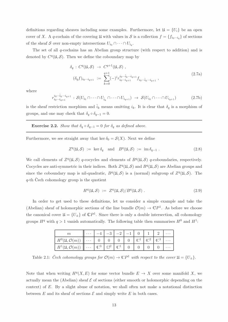
In order to get used to these definitions, let us consider a simple example and take the
(Abelian) sheaf of holomorphic sections of the line bundle O(m) → CP 1. As before we choose
the canonical cover U = U± of CP 1. Since there is only a double intersection, all cohomology
groups Hq with q > 1 vanish automatically. The following table then summarises H0 and H1:
m · · · −4 −3 −2 −1 0 1 2 · · ·H0(U,O(m)) · · · 0 0 0 0 C1 C2 C3 · · ·H1(U,O(m)) · · · C3 C2 C1 0 0 0 0 · · ·
Table 2.1: Cech cohomology groups for O(m)→ CP 1 with respect to the cover U = U±.
Note that when writing Hq(X,E) for some vector bundle E → X over some manifold X, we
actually mean the (Abelian) sheaf E of sections (either smooth or holomorphic depending on the
context) of E. By a slight abuse of notation, we shall often not make a notational distinction
between E and its sheaf of sections E and simply write E in both cases.
13
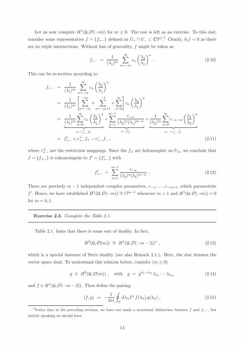
Let us now compute H1(U,O(−m)) for m ≥ 0. The rest is left as an exercise. To this end,
consider some representative f = f+− defined on U+ ∩ U− ⊂ CP 1.7 Clearly, δ1f = 0 as there
are no triple intersections. Without loss of generality, f might be taken as
f+− =1
(λ1)m
∞∑
n=−∞cn
(λ2λ1
)n
. (2.10)
This can be re-written according to
f+− =1
(λ1)m
∞∑
n=−∞cn
(λ2λ1
)n
=1
(λ1)m
[ −m∑
n=−∞+
−1∑
n=−m+1
+∞∑
n=0
]
cn
(λ2λ1
)n
=1
(λ1)m
∞∑
n=0
cn
(λ2λ1
)n
︸ ︷︷ ︸
=: r++−f+
+m−1∑
n=1
c−n(λ2)
n(λ1)m−n
︸ ︷︷ ︸
=: f ′+−
+1
(λ2)m
∞∑
n=0
c−n−m
(λ1λ2
)n
︸ ︷︷ ︸
=: −r−+−f−
= f ′+− + r++−f+ − r−+−f− , (2.11)
where r±+− are the restriction mappings. Since the f± are holomorphic on U±, we conclude that
f = f+− is cohomologous to f ′ = f ′+− with
f ′+− =
m−1∑
n=1
c−n(λ2)
n(λ1)m−n . (2.12)
There are precisely m − 1 independent complex parameters, c−1, . . . , c−m+1, which parametrise
f ′. Hence, we have established H1(U,O(−m)) ∼= Cm−1 whenever m > 1 and H1(U,O(−m)) = 0
for m = 0, 1.
Exercise 2.3. Complete the Table 2.1.
Table 2.1. hints that there is some sort of duality. In fact,
H0(U,O(m)) ∼= H1(U,O(−m− 2))∗ , (2.13)
which is a special instance of Serre duality (see also Remark 2.1.). Here, the star denotes the
vector space dual. To understand this relation better, consider (m ≥ 0)
g ∈ H0(U,O(m)) , with g = gα1···αmλα1 · · ·λαm (2.14)
and f ∈ H1(U,O(−m− 2)). Then define the pairing
(f, g) := − 1
2πi
∮
C
dλαλα f(λα) g(λα) , (2.15)
7Notice that in the preceding sections, we have not made a notational distinction between f and f+−, but
strictly speaking we should have.
14
where the contour is chosen as before. This expression is complex linear and non-degenerate and
depends only on the cohomology class of f . Hence, it gives the duality (2.13).
A nice way of writing (2.15) is as (f, g) = fα1···αmgα1···αm , where
fα1···αm := − 1
2πi
∮
C
dλαλα λα1 · · ·λαm f(λα) , (2.16)
such that Penrose’s contour integral formula (2.1) can be recognised as an instance of Serre duality
(the coordinate x being interpreted as some parameter).
Remark 2.1. If S is some Abelian sheaf over some compact complex manifold X with
covering U and K the sheaf of sections of the canonical line bundle K := detT ∗X, then
there is the following isomorphism which is referred to as Serre duality (or sometimes to as
Kodaira–Serre duality):
Hq(U,S) ∼= Hd−q(U,S∗ ⊗K)∗ .
Here, d = dimCX. See e.g. [9] for more details. In our present case, X = CP 1 and so
d = 1 and K = detT ∗CP 1 = T ∗CP 1 ∼= O(−2) and furthermore S = O(m).
One technical issue remains to be clarified. Apparently all of our above calculations seem to
depend on the chosen cover. But is this really the case?
Consider again some manifold X with cover U together with some Abelian sheaf S. If anothercover V is the refinement of U, that is, for U = Uii∈I and V = Vjj∈J there is a map ρ : J → I
of index sets, such that for any j ∈ J , Vj ⊆ Uρ(j), then there is a natural group homomorphism
(induced by the restriction mappings of the sheaf S)
hUV : Hq(U,S) → Hq(V,S) . (2.17)
We can then define the inductive limit of these cohomology groups with respect to the partially
ordered set of all coverings (see also Remark 2.2.),
Hq(X,S) := lim indU
Hq(U,S) (2.18)
which we call the q-th Cech cohomology group of X with coefficients in S.
Remark 2.2. Let us recall the definition of the inductive limit. If we let I be a partially
ordered set (with respect to ‘≥’) and Si a family of modules indexed by I with homomorph-
isms f ij : Si → Sj with i ≥ j and f ii = id, f ij f jk = f ik for i ≥ j ≥ k, then the inductive
limit,
lim indi∈I
Si ,
is defined by quotienting the disjoint union ˙⋃i∈ISi =
⋃
i∈I(i, Si) by the following equival-
ence relation: Two elements xi and xj of ˙⋃i∈ISi are said to be equivalent if there exists a
k ∈ I such that f ik(xi) = f jk(xj).
15

By the properties of inductive limits, we have a homomorphism Hq(U,S)→ Hq(X,S). Now the
question is: When does this becomes an isomorphism? The following theorem tells us when this
is going to happen.
Theorem 2.1. (Leray) Let U = Ui be a covering of X with the property that for all tuples
(Ui0 , . . . , Uip) of the cover, Hq(Ui0 ∩ · · · ∩ Uip ,S) = 0 for all q ≥ 1. Then
Hq(U,S) ∼= Hq(X,S) .
For a proof, see e.g. [10, 9].
Such covers are called Leray or acyclic covers and in fact our two-set cover U = U± of CP 1
is of this form. Therefore, Table 2.1. translates into Table 2.2.
m · · · −4 −3 −2 −1 0 1 2 · · ·H0(CP 1,O(m)) · · · 0 0 0 0 C1 C2 C3 · · ·H1(CP 1,O(m)) · · · C3 C2 C1 0 0 0 0 · · ·
Table 2.2: Cech cohomology groups for O(m)→ CP 1.
Remark 2.3. We have seen that twistor space P 3 ∼= CP 3 \CP 1 ∼= O(1)⊕O(1); see (1.17)
and (1.18). There is yet another interpretation. The Riemann sphere CP 1 can be embedded
into CP 3. The normal bundle NCP 1|CP 3 of CP 1 inside CP 3 is O(1)⊗O(1) as follows fromthe short exact sequence:
0ϕ1−→ TCP 1 ϕ2−→ TCP 3|CP 1
ϕ3−→ NCP 1|CP 3ϕ4−→ 0 .
Exactness of this sequence means that imϕi = kerϕi+1. If we take (zα, λα) as homogeneous
coordinates on CP 3 with the embedded CP 1 corresponding to zα = 0 and λα 6= 0, then
the non-trivial mappings ϕ2,3 are given by ϕ2 : ∂/∂λα 7→ ℓα∂/∂λα while ϕ3 : ℓα∂/∂zα +
ℓα∂/∂λα 7→ ℓα, where ℓα, ℓα are linear in zα, λα and the restriction to CP 1 is understood.
This shows that indeed NCP 1|CP 3∼= O(1) ⊗ O(1), i.e. twistor space P 3 can be identified
with the normal bundle of CP 1 → CP 3. Kodaira’s theorem on relative deformation states
that if Y is a compact complex submanifold of a not necessarily compact complex manifold
X, and if H1(Y,NY |X) = 0, where NY |X is the normal bundle of Y in X, then there exists
a d-dimensional family of deformations of Y inside X, where d := dimCH0(Y,NY |X). See
e.g. [11, 12] for more details. In our example, Y = CP 1, X = CP 3 and NCP 1|CP 3∼=
O(1) ⊗ O(1). Using Table 2.2., we conclude that H1(CP 1,O(1) ⊕ O(1)) = 0 and d = 4.
In fact, complex space-time M4 ∼= C4 is precisely this family of deformations. To be more
concrete, any Lx ∼= CP 1 has O(1)⊗C2 as normal bundle, and the tangent space TxM4 at
x ∈ M4 arises as TxM4 ∼= H0(Lx,O(1) ⊗ C2) ∼= H0(Lx,C2) ⊗ H0(Lx,O(1)) ∼= Sx ⊗ Sx,
where Sx := H0(Lx,C2) and Sx := H0(Lx,O(1)) which is the factorisation (1.12).
16

In summary, the functions f on twistor space from Section 2.1. leading to solutions of zero-
rest-mass field equations should be thought of as representatives of sheaf cohomology classes in
H1(P 3,O(∓2h− 2)). Then we can state the following theorem:
Theorem 2.2. (Penrose [7]) If we let Z±h be the sheaf of (sufficiently well-behaved) solutions to
the helicity ±h (with h ≥ 0) zero-rest-mass field equations on M4, then
H1(P 3,O(∓2h− 2)) ∼= H0(M4,Z±h) .
The proof of this theorem requires more work including a weightier mathematical machinery. It
therefore lies somewhat far afield from the main thread of development and we refer the interested
reader to e.g. [4] for details.
3. Self-dual Yang–Mills theory and the Penrose–Ward transform
So far, we have discussed free field equations. The subject of this section is a generalisation
of our above discussion to the non-linear field equations of self-dual Yang–Mills theory on four-
dimensional space-time. Self–dual Yang–Mills theory can be regarded as a subsector of Yang–
Mills theory and in fact, the self–dual Yang–Mills equations are the Bogomolnyi equations of
Yang–Mills theory. Solutions to the self-dual Yang–Mills equations are always solutions to the
Yang–Mills equations, while the converse may not be true.
3.1. Motivation
To begin with, let M4 be E and E → M4 a (complex) vector bundle over M4 with structure
group G. For the moment, we shall assume that G is semi-simple and compact. This allows us
to normalise the generators ta of G according to tr(t†atb) = −tr(tatb) = C(r)δab with C(r) > 0.
Furthermore, let ∇ : Ωp(M4, E)→ Ωp+1(M4, E) be a connection on E with curvature F = ∇2 ∈H0(M4,Ω2(M4,EndE)). Here, Ωp(M4) are the p-forms on M4 and Ωp(M4, E) := Ωp(M4)⊗ E.
Then ∇ = d + A and F = dA+ A ∧ A, where A is the EndE-valued connection one-form. The
reader unfamiliar with these quantities may wish to consult Appendix A. for their definitions. In
the coordinates xµ on M4 we have
A = dxµAµ and ∇ = dxµ∇µ , with ∇µ = ∂µ +Aµ (3.1a)
and therefore
F = 12dx
µ ∧ dxνFµν , with Fµν = [∇µ,∇ν ] = ∂µAν − ∂νAµ + [Aµ, Aν ] . (3.1b)
The Yang–Mills action functional is defined by
S = − 1
g2YM
∫
M4
tr(F ∧ ∗F ) , (3.2)
where gYM is the Yang–Mills coupling constant and ‘∗’ denotes the Hodge star on M4. The
corresponding field equations read as
∇∗F = 0 ⇐⇒ ∇µFµν = 0 . (3.3)
17
Exercise 3.1. Derive (3.3) by varying (3.2).
Solutions to the Yang–Mills equations are critical points of the Yang–Mills action. The critical
points may be local maxima of the action, local minima, or saddle points. To find the field
configurations that truly minimise (3.2), we consider the following inequality:
∓∫
M4
tr[(F ± ∗F ) ∧ (F ± ∗F )
]≥ 0 . (3.4)
A short calculation then shows that
−∫
M4
tr(F ∧ ∗F ) ≥ ±∫
M4
tr(F ∧ F ) (3.5)
and therefore
S ≥ ± 1
g2YM
∫
M4
tr(F ∧ F ) =⇒ S ≥ 8π2
g2YM
|Q| , (3.6)
where Q ∈ Z is called topological charge or instanton number,
Q = − 1
8π2
∫
M4
tr(F ∧ F ) = −c2(E) . (3.7)
Here, c2(E) denotes the second Chern class of E; see Appendix A. for the definition.
Equality is achieved for configurations that obey
F = ±∗F ⇐⇒ Fµν = ±12εµνλσF
λσ (3.8)
with εµνλσ = ε[µνλσ] and ε0123 = 1. These equations are called the self-dual and anti-self-
dual Yang–Mills equations. Solutions to these equations with finite charge Q are referred to as
instantons and anti-instantons. The sign of Q has been chosen such that Q > 0 for instantons
while Q < 0 for anti-instantons. Furthermore, by virtue of the Bianchi identity, ∇F = 0 ⇐⇒∇[µFνλ] = 0, solutions to (3.8) automatically satisfy the second-order Yang–Mills equations (3.3).
Remember from our discussion in Section 1.2. that the rotation group SO(4) is given by
SO(4) ∼= (SU(2)× SU(2))/Z2 . (3.9)
Therefore, the anti-symmetric tensor product of two vector representations 4 ∧ 4 decomposes
under this isomorphism as 4 ∧ 4 ∼= 3 ⊕ 3. More concretely, by taking the explicit isomorphism
(1.4), we can write
Fααββ := 14σ
µαασ
νββFµν = εαβfαβ + εαβfαβ , (3.10)
with fαβ = fβα and fαβ = fβα. Since each of these symmetric rank-2 tensors has three inde-
pendent components, we have made the decomposition 4 ∧ 4 ∼= 3 ⊕ 3 explicit. Furthermore, if
we write F = F+ + F− with F± := 12(F ± ∗F ), i.e. F± = ±∗F±, then
F+ ⇐⇒ fαβ and F− ⇐⇒ fαβ . (3.11)
Therefore, the self-dual Yang–Mills equations correspond to
F = ∗F ⇐⇒ F− = 0 ⇐⇒ fαβ = 0 (3.12)
and similarly for the anti-self-dual Yang–Mills equations.
18
Exercise 3.2. Verify (3.10) and (3.11) explicitly. Show further that F ∧ ∗F corresponds
to fαβfαβ + fαβf
αβ while F ∧ F to fαβfαβ − fαβf αβ.
Most surprisingly, even though they are non-linear, the (anti-)self-dual Yang–Mills equations
are integrable in the sense that one can give, at least in principle, all solutions. We shall establish
this by means of twistor geometry shortly, but again we will not be too rigorous in our discussion.
Furthermore, fαβ = 0 or fαβ = 0 make perfect sense in the complex setting. For convenience,
we shall therefore work in the complex setting from now on and impose reality conditions later
on when necessary. Notice that contrary to the Euclidean and Kleinian cases, the (anti-)self-dual
Yang–Mills equations on Minkowski space only make sense for complex Lie groups G. This is so
because ∗2 = −1 on two-forms in Minkowski space.
3.2. Penrose–Ward transform
The starting point is the double fibration (1.15), which we state again for the reader’s convenience,
P 3 M4
F 5
π1 π2
@@R
(3.13)
Consider now a rank-r holomorphic vector bundle E → P 3 together with its pull-back π∗1E → F 5.
Their structure groups are thus GL(r,C). We may impose the additional condition of having a
trivial determinant line bundle, detE, which reduces GL(r,C) to SL(r,C). Furthermore, we
again choose the two-patch covering U = U± of P 3. Similarly, F 5 may be covered by two
coordinate patches which we denote by U = U±. Therefore, E and π∗1E are characterised by
the transition functions f = f+− and π∗1f = π∗1f+−. As before, the pull-back of f+−(zα, λα)
is f+−(xαβλβ, λα), i.e. it is annihilated by the vector fields (1.14) and therefore constant along
π1 : F 5 → P 3. In the following, we shall not make a notational distinction between f and π∗1f
and simply write f for both bundles. Letting ∂P and ∂F be the anti-holomorphic parts of the
exterior derivatives on P 3 and F 5, respectively, we have π∗1 ∂P = ∂F π∗1 . Hence, the transition
function f+− is also annihilated by ∂F .
We shall also assume that E is holomorphically trivial when restricted to any projective line
Lx = π1(π−12 (x)) → P 3 for x ∈ M4. This then implies that there exist matrix-valued functions
ψ± on U±, which define trivialisations of π∗1E over U , such that f+− can be decomposed as (see
also Remark 3.1.)
f+− = ψ−1+ ψ− (3.14)
with ∂Fψ± = 0, i.e. the ψ± = ψ±(x, λ±) are holomorphic on U±. Clearly, this splitting is not
unique, since one can always perform the transformation
ψ± 7→ g−1 ψ± , (3.15)
19
where g is some globally defined matrix-valued function holomorphic function on F 5. Hence, it
is constant on CP 1, i.e. it depends on x but not on λ±. We shall see momentarily, what the
transformation (3.15) corresponds to on space-time M4.
Since V ±α f+− = 0, where V ±
α are the restrictions of the vector fields Vα given in (1.14) to the
coordinate patches U±, we find
ψ+V+α ψ
−1+ = ψ−V +
α ψ−1− (3.16)
on U+ ∩ U−. Explicitly, V ±α = λβ±∂αβ with λ+α := λα/λ1 = (1, λ+)
t and λ−α := λα/λ2 = (λ−, 1)t.
Therefore, by an extension of Liouville’s theorem, the expressions (3.16) can be at most linear in
λ+. This can also be understood by noting
ψ+V+α ψ
−1+ = ψ−V
+α ψ
−1− = λ+ψ−V
−α ψ
−1− (3.17)
and so it is of homogeneity 1. Thus, we may introduce a Lie algebra-valued one-form A on F 5
which has components only along π1 : F 5 → P 3,
VαyA|U±:= A±
α = ψ±V±α ψ
−1± = λβ±Aαβ , (3.18)
where Aαβ is λ±-independent. This can be re-written as
(V ±α +A±
α )ψ± = λβ±∇αβψ± = 0 , with ∇αβ := ∂αβ +Aαβ . (3.19)
The compatibility conditions for this linear system read as
[∇αα,∇ββ] + [∇αβ ,∇βα] = 0 , (3.20)
which is equivalent to saying that the fαβ-part of
[∇αα,∇ββ] = εαβfαβ + εαβfαβ (3.21)
vanishes. However, fαβ = 0 is nothing but the self-dual Yang–Mills equations (3.12) on M4.
Notice that the transformations of the form (3.15) induce the transformations
Aαβ 7→ g−1∂αβg + g−1Aαβg (3.22)
of Aαβ as can be seen directly from (3.19). Hence, these transformations induce gauge trans-
formations on space-time and so we may define gauge equivalence classes [Aαβ ], where two gauge
potentials are said to be equivalent if they differ by a transformation of the form (3.22). On the
other hand, transformations of the form8
f+− 7→ h−1+ f+−h− , (3.23)
where h± are matrix-valued functions holomorphic on U± with V ±α h± = 0, leave the gauge
potential Aαβ invariant. Since V ±α h± = 0, the functions h± descend down to twistor space P 3
8In Section 5.2., we will formalise these transformations in the framework of non-Abelian sheaf cohomology.
20

and are holomorphic on U± (remember that any function on twistor space that is pulled back to
the correspondence space must be annihilated by the vector fields Vα). Two transition functions
that differ by a transformation of the form (3.23) are then said to be equivalent, as they define
two holomorphic vector bundles which are bi-holomorphic. Therefore, we may conclude that an
equivalence class [f+−] corresponds to an equivalence class [Aαβ ].
Altogether, we have seen that holomorphic vector bundles E → P 3 over twistor space, which
are holomorphically trivial on all projective lines Lx → P 3 yield solutions of the self-dual Yang–
Mills equations onM4. In fact, the converse is also true: Any solution to the self-dual Yang–Mills
equations arises in this way. See e.g. [4] for a complete proof. Therefore, we have:
Theorem 3.1. (Ward [13]) There is a one-to-one correspondence between gauge equivalence
classes of solutions to the self-dual Yang–Mills equations on M4 and equivalence classes of holo-
morphic vector bundles over the twistor space P 3 which are holomorphically trivial on any pro-
jective line Lx = π1(π−12 (x)) → P 3.
Hence, all solutions to the self-dual Yang–Mills equations are encoded in these vector bundles and
once more, differentially constrained data on space-time (the gauge potential Aαβ) is encoded in
differentially unconstrained complex analytic data (the transition function f+−) on twistor space.
The reader might be worried that our constructions depend on the choice of coverings, but as in
the case of the Penrose transform, this is not the case as will become transparent in Section 5.2.
As before, one may also write down certain integral formulæ for the gauge potential Aαβ . In
addition, given a solution A = dxαβAαβ to the self-dual Yang–Mills equations, the matrix-valued
functions ψ± are given by
ψ± = Pexp
(
−∫
C±
A
)
, (3.24)
where ‘P’ denotes the path-ordering symbol and the contour C± is any real curve in the null-plane
π2(π−11 (p)) →M4 for p ∈ P 3 running from some point x0 to a point x with xαβ(s) = xαβ0 +sµαλα±
for s ∈ [0, 1] and constant µα; the choice of contour plays no role, since the curvature is zero when
restricted to the null-plane.
Exercise 3.3. Show that for a rank-1 holomorphic vector bundle E → P 3, the Ward the-
orem coincides with the Penrose transform for a helicity h = −1 field. See also Appendix D.
Thus, the Ward theorem gives a non-Abelian generalisation of that case and one therefore
often speaks of the Penrose–Ward transform.
Before giving an explicit example of a real instanton solution, let us say a few words about
real structures. In Section 1.2., we introduced reality conditions on M4 leading to Euclidean,
Minkowski and Kleinian spaces. In fact, these conditions are induced from twistor space as we
shall now explain. For concreteness, let us restrict our attention to the Euclidean case. The
Kleinian case will be discussed in Section 8.3. Remember that a Minkowski signature does not
allow for real (anti-)instantons.
21
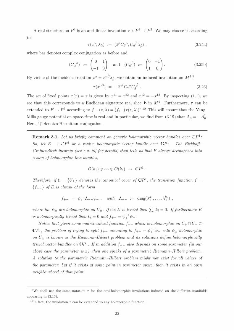
A real structure on P 3 is an anti-linear involution τ : P 3 → P 3. We may choose it according
to:
τ(zα, λα) := (zβCβα, Cα
βλβ) , (3.25a)
where bar denotes complex conjugation as before and
(Cαβ) :=
(
0 1
−1 0
)
and (Cαβ) :=
(
0 −11 0
)
. (3.25b)
By virtue of the incidence relation zα = xαβλβ, we obtain an induced involution on M4,9
τ(xαβ) = −xγδCγαCδ β . (3.26)
The set of fixed points τ(x) = x is given by x11 = x22 and x12 = −x12. By inspecting (1.1), we
see that this corresponds to a Euclidean signature real slice E in M4. Furthermore, τ can be
extended to E → P 3 according to f+−(z, λ) = (f+−(τ(z, λ))†.10 This will ensure that the Yang–
Mills gauge potential on space-time is real and in particular, we find from (3.19) that Aµ = −A†µ.
Here, ‘†’ denotes Hermitian conjugation.
Remark 3.1. Let us briefly comment on generic holomorphic vector bundles over CP 1:
So, let E → CP 1 be a rank-r holomorphic vector bundle over CP 1. The Birkhoff–
Grothendieck theorem (see e.g. [9] for details) then tells us that E always decomposes into
a sum of holomorphic line bundles,
O(k1)⊕ · · · ⊕ O(kr) → CP 1 .
Therefore, if U = U± denotes the canonical cover of CP 1, the transition function f =
f+− of E is always of the form
f+− = ψ−1+ Λ+−ψ− , with Λ+− := diag(λk1+ , . . . , λ
kr+ ) ,
where the ψ± are holomorphic on U±. If detE is trivial then∑
i ki = 0. If furthermore E
is holomorpically trivial then ki = 0 and f+− = ψ−1+ ψ−.
Notice that given some matrix-valued function f+− which is holomorphic on U+ ∩U− ⊂CP 1, the problem of trying to split f+− according to f+− = ψ−1+ ψ− with ψ± holomorphic
on U± is known as the Riemann–Hilbert problem and its solutions define holomorphically
trivial vector bundles on CP 1. If in addition f+− also depends on some parameter (in our
above case the parameter is x), then one speaks of a parametric Riemann–Hilbert problem.
A solution to the parametric Riemann–Hilbert problem might not exist for all values of
the parameter, but if it exists at some point in parameter space, then it exists in an open
neighbourhood of that point.
9We shall use the same notation τ for the anti-holomorphic involutions induced on the different manifolds
appearing in (3.13).10In fact, the involution τ can be extended to any holomorphic function.
22
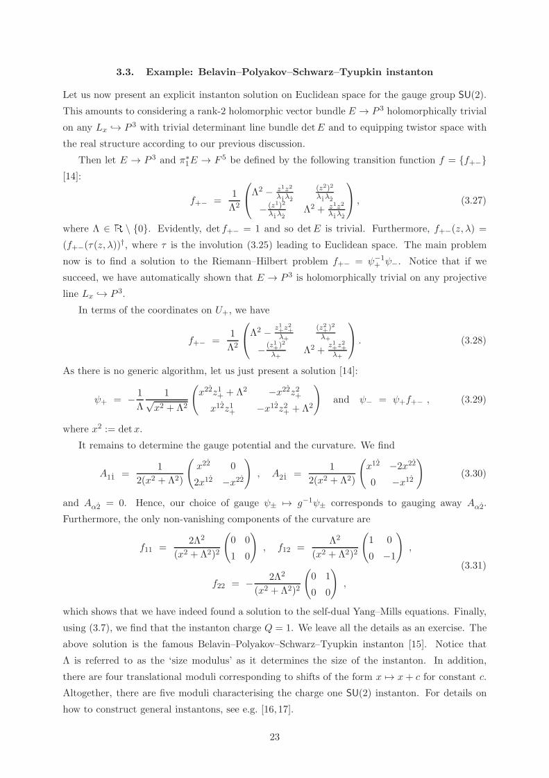
3.3. Example: Belavin–Polyakov–Schwarz–Tyupkin instanton
Let us now present an explicit instanton solution on Euclidean space for the gauge group SU(2).
This amounts to considering a rank-2 holomorphic vector bundle E → P 3 holomorphically trivial
on any Lx → P 3 with trivial determinant line bundle detE and to equipping twistor space with
the real structure according to our previous discussion.
Then let E → P 3 and π∗1E → F 5 be defined by the following transition function f = f+−[14]:
f+− =1
Λ2
Λ2 − z1z2
λ1λ2
(z2)2
λ1λ2
− (z1)2
λ1λ2Λ2 + z1z2
λ1λ2
, (3.27)
where Λ ∈ R \ 0. Evidently, det f+− = 1 and so detE is trivial. Furthermore, f+−(z, λ) =
(f+−(τ(z, λ))†, where τ is the involution (3.25) leading to Euclidean space. The main problem
now is to find a solution to the Riemann–Hilbert problem f+− = ψ−1+ ψ−. Notice that if we
succeed, we have automatically shown that E → P 3 is holomorphically trivial on any projective
line Lx → P 3.
In terms of the coordinates on U+, we have
f+− =1
Λ2
Λ2 − z1+z
2+
λ+
(z2+)2
λ+
− (z1+)2
λ+Λ2 +
z1+z2+
λ+
. (3.28)
As there is no generic algorithm, let us just present a solution [14]:
ψ+ = − 1
Λ
1√x2 + Λ2
(
x22z1+ + Λ2 −x22z2+x12z1+ −x12z2+ + Λ2
)
and ψ− = ψ+f+− , (3.29)
where x2 := detx.
It remains to determine the gauge potential and the curvature. We find
A11 =1
2(x2 + Λ2)
(
x22 0
2x12 −x22
)
, A21 =1
2(x2 + Λ2)
(
x12 −2x22
0 −x12
)
(3.30)
and Aα2 = 0. Hence, our choice of gauge ψ± 7→ g−1ψ± corresponds to gauging away Aα2.
Furthermore, the only non-vanishing components of the curvature are
f11 =2Λ2
(x2 +Λ2)2
(
0 0
1 0
)
, f12 =Λ2
(x2 +Λ2)2
(
1 0
0 −1
)
,
f22 = − 2Λ2
(x2 + Λ2)2
(
0 1
0 0
)
,
(3.31)
which shows that we have indeed found a solution to the self-dual Yang–Mills equations. Finally,
using (3.7), we find that the instanton charge Q = 1. We leave all the details as an exercise. The
above solution is the famous Belavin–Polyakov–Schwarz–Tyupkin instanton [15]. Notice that
Λ is referred to as the ‘size modulus’ as it determines the size of the instanton. In addition,
there are four translational moduli corresponding to shifts of the form x 7→ x+ c for constant c.
Altogether, there are five moduli characterising the charge one SU(2) instanton. For details on
how to construct general instantons, see e.g. [16, 17].
23
Exercise 3.4. Show that (3.29) implies (3.30) and (3.31) by using the linear system (3.19).
Furthermore, show that Q = 1. You might find the following integral useful:
∫E d4x
(x2 + Λ2)4=
π2
6Λ4,
where x2 = xµxµ.
4. Supertwistor space
Up to now, we have discussed the purely bosonic setup. As our goal is the construction of amp-
litudes in supersymmetric gauge theories, we need to incorporate fermionic degrees of freedom.
To this end, we start by briefly discussing supermanifolds before we move on and introduce su-
pertwistor space and the supersymmetric generalisation of the self-dual Yang–Mills equations.
For a detailed discussion about supermanifolds, we refer to [18–20].
4.1. A brief introduction to supermanifolds
Let R ∼= R0 ⊕ R1 be a Z2-graded ring, that is, R0R0 ⊂ R0, R1R0 ⊂ R1, R0R1 ⊂ R1 and
R1R1 ⊂ R0. We call elements of R0 Graßmann even (or bosonic) and elements of R1 Graßmann
odd (or fermionic). An element of R is said to be homogeneous if it is either bosonic or fermionic.
The degree (or Graßmann parity) of a homogeneous element is defined to be 0 if it is bosonic and
1 if it is fermionic, respectively. We denote the degree of a homogeneous element r ∈ R by pr (p
for parity).
We define the supercommutator, [·, · : R×R→ R, by
[r1, r2 := r1r2 − (−)pr1pr2 r2r1 , (4.1)
for all homogeneous elements r1,2 ∈ R. The Z2-graded ring R is called supercommutative if the
supercommutator vanishes for all of the ring’s elements. For our purposes, the most important
example of such a supercommutative ring is the Graßmann or exterior algebra over Cn,R = Λ•Cn :=
⊕
p
ΛpCn , (4.2a)
with the Z2-grading being
R =⊕
p
Λ2pCn︸ ︷︷ ︸
=: R0
⊕⊕
p
Λ2p+1Cn︸ ︷︷ ︸
=: R1
. (4.2b)
An R-module M is a Z2-graded bi-module which satisfies
rm = (−)prpmmr , (4.3)
24
for homogeneous r ∈ R, m ∈ M , with M ∼= M0 ⊕M1. Then there is a natural map11 Π, called
the parity operator, which is defined by
(ΠM)0 := M1 and (ΠM)1 := M0 . (4.4)
We should stress that R is an R-module itself, and as such ΠR is an R-module, as well. However,
ΠR is no longer a Z2-graded ring since (ΠR)1(ΠR)1 ⊂ (ΠR)1, for instance.
A free module of rank m|n over R is defined by
Rm|n := Rm ⊕ (ΠR)n , (4.5)
where Rm := R ⊕ · · · ⊕ R. This has a free system of generators, m of which are bosonic and
n of which are fermionic, respectively. We stress that the decomposition of Rm|n into Rm|0 and
R0|n has, in general, no invariant meaning and does not coincide with the decomposition into
bosonic and fermionic parts, [Rm0 ⊕ (ΠR1)n] ⊕ [Rm1 ⊕ (ΠR0)
n]. Only when R1 = 0, are these
decompositions the same. An example is Cm|n, where we consider the complex numbers as aZ2-graded ring (where R = R0 with R0 = C and R1 = 0).
Let R be a supercommutative ring and Rm|n be a freely generated R-module. Just as in the
commutative case, morphisms between free R-modules can be given by matrices. The standard
matrix format is
A =
(
A1 A2
A3 A4
)
, (4.6)
where A is said to be bosonic (respectively, fermionic) if A1 and A4 are filled with bosonic (re-
spectively, fermionic) elements of the ring while A2 and A3 are filled with fermionic (respectively,
bosonic) elements. Furthermore, A1 is a p×m-, A2 a q×m-, A3 a p×n- and A4 a q×n-matrix.
The set of matrices in standard format with elements in R is denoted by Mat(m|n, p|q,R). It
forms a Z2-graded module which, with the usual matrix multiplication, is naturally isomorphic
to Hom(Rm|n, Rp|q). We denote the endomorphisms of Rm|n by End(m|n,R) and the automorph-
isms by Aut(m|n,R), respectively. We use further the special symbols gl(m|n,R) ⊂ End(m|n,R)to denote the bosonic endomorphisms of Rm|n and GL(m|n,R) ⊂ Aut(m|n,R) to denote the
bosonic automorphisms.
The supertranspose of A ∈ Mat(m|n, p|q,R) is defined according to
Ast :=
(
At1 (−)pA At
3
−(−)pAAt2 At
4
)
, (4.7)
where the superscript ‘t’ denotes the usual transpose. The supertransposition satisfies (A+B)st =
Ast+Bst and (AB)st = (−)pApBBstAst. We shall use the following definition of the supertrace of
A ∈ End(m|n,R):strA := trA1 − (−)pAtrA4 . (4.8)
11More precisely, it is a functor from the category of R-modules to the category of R-modules. See Appendix
C. for details.
25

The supercommutator for matrices is defined analogously to (4.1), i.e. [A,B := AB−(−)pApBBAfor A,B ∈ End(m|n,R). Then str[A,B = 0 and strAst = strA. Finally, let A ∈ GL(m|n,R).The superdeterminant is given by
sdetA := det(A1 −A2A−14 A3) detA
−14 , (4.9)
where the right-hand side is well-defined for A1 ∈ GL(m|0, R0) and A4 ∈ GL(n|0, R0). Further-
more, it belongs to GL(1|0, R0). The superdeterminant satisfies the usual rules, sdet(AB) =
sdetA sdetB and sdetAst = sdetA for A,B ∈ GL(m|n,R). Notice that sometimes sdet is referred
to as the Berezinian and also denoted by Ber.
After this digression, we may now introduce the local model of a supermanifold. Let V be an
open subset in Cm and consider OV (Λ•Cn) := OV ⊗Λ•Cn , where OV is the sheaf of holomorphic
functions on V ⊂ Cm which is also referred to as the structure sheaf of V . Thus, OV (Λ•Cn) is asheaf of supercommutative rings consisting of Λ•Cn-valued holomorphic functions on V . Let now
(x1, . . . , xm) be coordinates on V ⊂ Cm and (η1, . . . , ηn) be a basis of the sections of Cn ∼= Λ1Cn.Then (x1, . . . , xm, η1, . . . , ηn) are coordinates for the ringed space V m|n := (V,OV (Λ•Cn)). Any
function f can thus be Taylor-expanded as
f(x, η) =∑
I
ηIfI(x) , (4.10)
where I is a multi-index. These are the fundamental functions in supergeometry.
To define a general supermanifold, let X be some topological space of real dimension 2m, and
let RX be a sheaf of supercommutative rings on X. Furthermore, let N be the ideal subsheaf
in RX of all nil-potent elements in RX , and define OX := RX/N .12 Then Xm|n := (X,RX ) is
called a complex supermanifold of dimension m|n if the following is fulfilled:
(i) Xm := (X,OX ) is an m-dimensional complex manifold which we call the body of Xm|n.
(ii) For each point x ∈ X there is a neighbourhood U ∋ x such that there is a local isomorphism
RX |U ∼= OX(Λ•(N/N 2))|U , whereN/N 2 is a rank-n locally free sheaf ofOX -modules onX,
i.e. N/N 2 is locally of the form OX ⊕· · ·⊕OX (n-times); N/N 2 is called the characteristic
sheaf of Xm|n.
Therefore, complex supermanifolds look locally like V m|n = (V,OV (Λ•Cn)). In view of this,
we picture Cm|n as (Cm,OCm(Λ•Cn)). We shall refer to RX as the structure sheaf of the
supermanifold Xm|n and to OX as the structure sheaf of the body Xm of Xm|n. Later on, we
shall use a more common notation and re-denoteRX by OX or simply by O if there is no confusion
with the structure sheaf of the body Xm of Xm|n. In addition, we sometimes write Xm|0 instead
of Xm. Furthermore, the tangent bundle TXm|n of a complex supermanifold Xm|n is an example
of a supervector bundle, where the transition functions are sections of the (non-Abelian) sheaf
GL(m|n,RX) (see Section 5.2. for more details).
12Instead of RX , one often also writes R and likewise for OX .
26
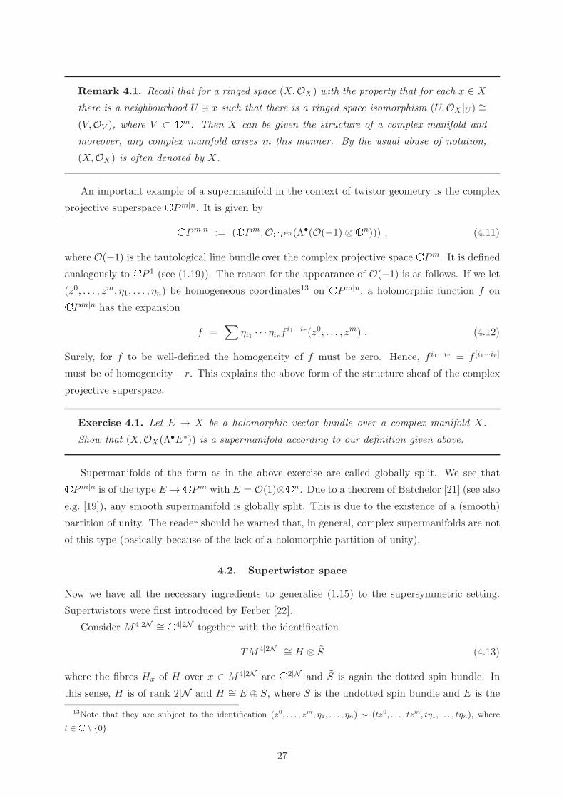
Remark 4.1. Recall that for a ringed space (X,OX ) with the property that for each x ∈ Xthere is a neighbourhood U ∋ x such that there is a ringed space isomorphism (U,OX |U ) ∼=(V,OV ), where V ⊂ Cm. Then X can be given the structure of a complex manifold and
moreover, any complex manifold arises in this manner. By the usual abuse of notation,
(X,OX ) is often denoted by X.
An important example of a supermanifold in the context of twistor geometry is the complex
projective superspace CPm|n. It is given byCPm|n := (CPm,OCPm(Λ•(O(−1) ⊗Cn))) , (4.11)
where O(−1) is the tautological line bundle over the complex projective space CPm. It is definedanalogously to CP 1 (see (1.19)). The reason for the appearance of O(−1) is as follows. If we let
(z0, . . . , zm, η1, . . . , ηn) be homogeneous coordinates13 on CPm|n, a holomorphic function f onCPm|n has the expansion
f =∑
ηi1 · · · ηirf i1···ir(z0, . . . , zm) . (4.12)
Surely, for f to be well-defined the homogeneity of f must be zero. Hence, f i1···ir = f [i1···ir ]
must be of homogeneity −r. This explains the above form of the structure sheaf of the complex
projective superspace.
Exercise 4.1. Let E → X be a holomorphic vector bundle over a complex manifold X.
Show that (X,OX (Λ•E∗)) is a supermanifold according to our definition given above.
Supermanifolds of the form as in the above exercise are called globally split. We see thatCPm|n is of the type E → CPm with E = O(1)⊗Cn. Due to a theorem of Batchelor [21] (see also
e.g. [19]), any smooth supermanifold is globally split. This is due to the existence of a (smooth)
partition of unity. The reader should be warned that, in general, complex supermanifolds are not
of this type (basically because of the lack of a holomorphic partition of unity).
4.2. Supertwistor space
Now we have all the necessary ingredients to generalise (1.15) to the supersymmetric setting.
Supertwistors were first introduced by Ferber [22].
Consider M4|2N ∼= C4|2N together with the identification
TM4|2N ∼= H ⊗ S (4.13)
where the fibres Hx of H over x ∈ M4|2N are C2|N and S is again the dotted spin bundle. In
this sense, H is of rank 2|N and H ∼= E ⊕ S, where S is the undotted spin bundle and E is the
13Note that they are subject to the identification (z0, . . . , zm, η1, . . . , ηn) ∼ (tz0, . . . , tzm, tη1, . . . , tηn), where
t ∈ C \ 0.
27

rank-0|N R-symmetry bundle. In analogy to xµ ↔ xαβ , we now have xM ↔ xAα = (xαα, ηαi )
for A = (α, i), B = (β, j), . . . and i, j, . . . = 1, . . . ,N . Notice that the above factorisation of the
tangent bundle can be understood as a generalisation of a conformal structure (see Remark 1.1.)
known as para-conformal structure (see e.g. [23]).
As in the bosonic setting, we may consider the projectivisation of S∗ to define the correspond-
ence space F 5|2N := P(S∗) ∼= C4|2N ×CP 1. Furthermore, we consider the vector fields
VA = λα∂Aα = λα∂
∂xAα. (4.14)
They define an integrable rank-2|N distribution on the correspondence space. The resulting
quotient will be supertwistor P 3|N :
P 3|N M4|2N
F 5|2Nπ1 π2
@@R
(4.15)
The projection π2 is the trivial projection and π1 : (xAα, λα) 7→ (zA, λα) = (xAαλα, λα), where
(zA, λα) = (zα, ηi, λα) are homogeneous coordinates on P 3|N .
As before, we may cover P 3|N by two coordinate patches, which we (again) denote by U±:
U+ : λ1 6= 0 and zA+ :=zA
λ1and λ+ :=
λ2λ1
,
U− : λ2 6= 0 and zA− :=zA
λ2and λ− :=
λ1λ2
.
(4.16)
On U+ ∩ U− we have zA+ = λ+zA− and λ+ = λ−1
− . This shows that P 3|N can be identified withCP 3|N \CP 1|N . It can also be identified with the total space of the holomorphic fibration
O(1)⊗C2|N → CP 1 . (4.17)
Another way of writing this is O(1)⊗C2⊕ΠO(1)⊗CN → CP 1, where Π is the parity map given
in (4.4). In the following, we shall denote the two patches covering the correspondence space
F 5|2N by U±. Notice that Remark 2.3. also applies to P 3|N .
Similarly, we may extend the geometric correspondence: A point x ∈ M4|2N corresponds to
a projective line Lx = π1(π−12 (x)) → P 3|N , while a point p = (z, λ) ∈ P 3|N corresponds to a
2|N -plane in superspace-time M4|2N that is parametrised by xAα = xAα0 + µAλα, where xAα0 is a
particular solution to the supersymmetric incidence relation zA = xAαλα.
4.3. Superconformal algebra
Before we move on and talk about supersymmetric extensions of self-dual Yang–Mills theory, let
us digress a little and collect a few facts about the superconformal algebra. The conformal algebra,
conf4, in four dimensions is a real form of the complex Lie algebra sl(4,C). The concrete real
form depends on the choice of signature of space-time. For Euclidean signature we have so(1, 5) ∼=su∗(4) while for Minkowski and Kleinian signatures we have so(2, 4) ∼= su(2, 2) and so(3, 3) ∼=sl(4,R), respectively. Likewise, the N -extended conformal algebra—the superconformal algebra,
conf4|N—is a real form of the complex Lie superalgebra sl(4|N ,C) for N < 4 and psl(4|4,C) for28
N = 4. For a compendium of Lie superalgebras, see e.g. [24]. In particular, for N < 4 we have
su∗(4|N ), su(2, 2|N ) and sl(4|N ,R) for Euclidean, Minkowski and Kleinian signatures while for
N = 4 the superconformal algebras are psu∗(4|4), psu(2, 2|4) and psl(4|4,R). Notice that for a
Euclidean signature, the number N of supersymmetries is restricted to be even.
The generators of conf4|N are
conf4|N = spanPµ, Lµν ,K
µ,D,Rij, A |Qiα, Qiα, Siα, Sαi
. (4.18)
Here, Pµ represents translations, Lµν (Lorentz) rotations, Kµ special conformal transformations,
D dilatations and Rij the R-symmetry while Qiα, Q
iα are the Poincare supercharges and Siα,
Sαi their superconformal partners. Furthermore, A is the axial charge which absent for N = 4.
Making use of the identification (1.12), we may also write
conf4|N = spanPαβ , Lαβ , Lαβ,K
αβ,D,Rij , A |Qiα, Qiα, Siα, Sαi
, (4.19)
where the Lαβ , Lαβ are symmetric in their indices (see also (3.10)). We may also include a central
extension z = spanZ leading to conf4|N ⊕ z, i.e. [conf4|N , z = 0 and [z, z = 0.
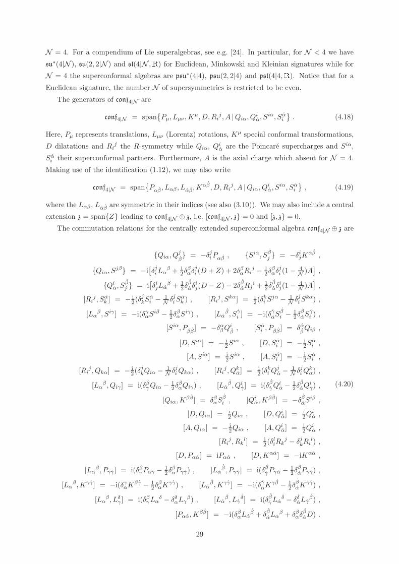
The commutation relations for the centrally extended superconformal algebra conf4|N ⊕ z are
Qiα, Qjβ = −δjiPαβ , Siα, Sβj = −δijKαβ ,
Qiα, Sjβ = −i[δjiLα
β + 12δβαδ
ji (D + Z) + 2δβαRi
j − 12δβαδ
ji (1− 4
N )A],
Qiα, Sβj = i[δijLα
β + 12δβαδ
ij(D − Z)− 2δβαRj
i + 12δβαδ
ij(1− 4
N )A],
[Rij, Sαk ] = − i
2(δjkS
αi − 1
N δjiS
αk ) , [Ri
j , Skα] = i2(δ
ki S
jα − 1N δ
jiS
kα) ,
[Lαβ, Siγ ] = −i(δγαSiβ − 1
2δβαS
iγ) , [Lαβ, Sγi ] = −i(δγαS
βi − 1
2δβαS
γi ) ,
[Siα, Pββ ] = −δαβQiβ , [Sαi , Pββ ] = δαβQiβ ,
[D,Siα] = − i2S
iα , [D,Sαi ] = − i2S
αi ,
[A,Siα] = i2S
iα , [A,Sαi ] = − i2S
αi ,
[Rij , Qkα] = − i
2(δjkQiα − 1
N δjiQkα) , [Ri
j, Qkα] = i2(δ
ki Q
jα − 1
N δjiQ
kα) ,
[Lαβ , Qiγ ] = i(δβγQiα − 1
2δβαQiγ) , [Lα
β , Qiγ ] = i(δβγQiα − 1
2δβαQ
iγ) ,
[Qiα,Kββ ] = δβαS
βi , [Qiα,K
ββ] = −δβαSiβ ,[D,Qiα] = i
2Qiα , [D,Qiα] = i2Q
iα ,
[A,Qiα] = − i2Qiα , [A,Qiα] = i
2Qiα ,
[Rij , Rk
l] = i2(δ
liRk
j − δjkRil) ,[D,Pαα] = iPαα , [D,Kαα] = −iKαα ,
[Lαβ, Pγγ ] = i(δβγPαγ − 1
2δβαPγγ) , [Lα
β, Pγγ ] = i(δβγPγα − 12δβαPγγ) ,
[Lαβ,Kγγ ] = −i(δγαKβγ − 1
2δβαK
γγ) , [Lαβ,Kγγ ] = −i(δγαKγβ − 1
2δβαK
γγ) ,
[Lαβ, Lδγ ] = i(δβγLα
δ − δδαLγβ) , [Lαβ, Lγ
δ] = i(δβγLαδ − δδαLγ β) ,
[Pαα,Kββ] = −i(δβαLαβ + δβαLα
β + δβαδβαD) .
(4.20)
29
Notice that for N = 4, the axial charge A decouples, as mentioned above. Notice also that upon
chosing a real structure, not all of the above commutation relations are independent of each other.
Some of them will be related via conjugation.
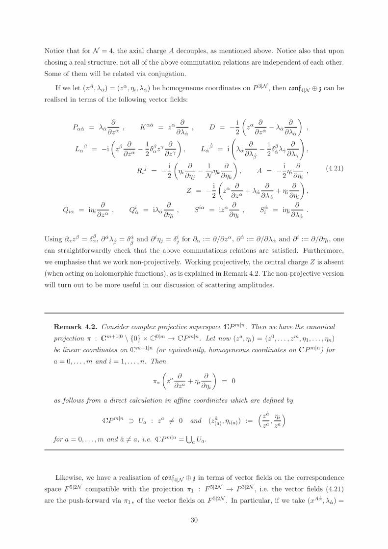
If we let (zA, λα) = (zα, ηi, λα) be homogeneous coordinates on P 3|N , then conf4|N ⊕ z can be
realised in terms of the following vector fields:
Pαα = λα∂
∂zα, Kαα = zα
∂
∂λα, D = − i
2
(
zα∂
∂zα− λα
∂
∂λα
)
,
Lαβ = −i
(
zβ∂
∂zα− 1
2δβαz
γ ∂
∂zγ
)
, Lαβ = i
(
λα∂
∂λβ− 1
2δβαλγ
∂
∂λγ
)
,
Rij = − i
2
(
ηi∂
∂ηj− 1
N ηk∂
∂ηk
)
, A = − i
2ηi
∂
∂ηi,
Z = − i
2
(
zα∂
∂zα+ λα
∂
∂λα+ ηi
∂
∂ηi
)
,
Qiα = iηi∂
∂zα, Qiα = iλα
∂
∂ηi, Siα = izα
∂
∂ηi, Sαi = iηi
∂
∂λα.
(4.21)
Using ∂αzβ = δβα, ∂αλβ = δα
βand ∂iηj = δij for ∂α := ∂/∂zα, ∂α := ∂/∂λα and ∂i := ∂/∂ηi, one
can straightforwardly check that the above commutations relations are satisfied. Furthermore,
we emphasise that we work non-projectively. Working projectively, the central charge Z is absent
(when acting on holomorphic functions), as is explained in Remark 4.2. The non-projective version
will turn out to be more useful in our discussion of scattering amplitudes.
Remark 4.2. Consider complex projective superspace CPm|n. Then we have the canonical
projection π : Cm+1|0 \ 0 × C0|m → CPm|n. Let now (za, ηi) = (z0, . . . , zm, η1, . . . , ηn)
be linear coordinates on Cm+1|n (or equivalently, homogeneous coordinates on CPm|n) for
a = 0, . . . ,m and i = 1, . . . , n. Then
π∗
(
za∂
∂za+ ηi
∂
∂ηi
)
= 0
as follows from a direct calculation in affine coordinates which are defined byCPm|n ⊃ Ua : za 6= 0 and (za(a), ηi(a)) :=(za
za,ηiza
)
for a = 0, . . . ,m and a 6= a, i.e. CPm|n =⋃
a Ua.
Likewise, we have a realisation of conf4|N ⊕ z in terms of vector fields on the correspondence
space F 5|2N compatible with the projection π1 : F 5|2N → P 3|2N , i.e. the vector fields (4.21)
are the push-forward via π1 ∗ of the vector fields on F 5|2N . In particular, if we take (xAα, λα) =
30

(xαα, ηαi , λα) as coordinates on F5|2N , where λα are homogeneous coordinates on CP 1, we have
Pαα =∂
∂xαα, Kαα = −xαβxβα ∂
∂xββ− xαβηαi
∂
∂ηβi
+ xαβλβ∂
∂λα,
D = −i(
xαα∂
∂xαα+
1
2ηαi
∂
∂ηαi− 1
2λα
∂
∂λα
)
,
Lαβ = −i
(
xββ∂
∂xαβ− 1
2δβαx
γγ ∂
∂xγγ
)
,
Lαβ = −i
(
xββ∂
∂xβα− 1
2δβαx
γγ ∂
∂xγγ
)
− i
(
ηβi∂
∂ηαi− 1
2δβαη
γk
∂
∂ηγk
)
+ i
(
λα∂
∂λα− 1
2δβαλγ
∂
∂λγ
)
,
Rij = − i
2
(
ηαi∂
∂ηαj− 1
N ηαk∂
∂ηαk
)
, A = − i
2ηαi
∂
∂ηαi, Z = − i
2λα
∂
∂λα,
Qiα = iηαi∂
∂xαα, Qiα = i
∂
∂ηαi,
Siα = ixαα∂
∂ηαi, Sαi = −iηβi xβα
∂
∂xββ− iηβi η
αj
∂
∂ηβj
+ iηβi λβ∂
∂λα.
(4.22)
In order to understand these expressions, let us consider a holomorphic function f on F 5|2N
which descends down to P 3|N . Recall that such a function is of the form f = f(xAαλα, λα) =
f(xααλα, ηαi λα, λα) since then VAf = 0. Then
∂
∂xAα
∣∣∣∣λα
f = λα∂
∂zA
∣∣∣∣λα
f ,
∂
∂λα
∣∣∣∣xAα
f =
(
xAα∂
∂zA
∣∣∣∣λα
+∂
∂λα
∣∣∣∣zA
)
f .
(4.23)
Next let us exemplify the calculation for the generator Lαβ. The rest is left as an exercise. Using
the relations (4.23), we find
[
−i(
xAβ∂
∂xAα− 1
2δβαx
Cγ ∂
∂xCγ
)∣∣∣∣λα
+ i
(
λα∂
∂λβ− 1
2δβαλγ
∂
∂λγ
)∣∣∣∣∣xAα
]
f =
= i
(
λα∂
∂λβ− 1
2δβαλγ
∂
∂λγ
)∣∣∣∣∣zA
f .
(4.24)
Therefore,
π1 ∗
[
−i(
xAβ∂
∂xAα− 1
2δβαx
Cγ ∂
∂xCγ
)
+ i
(
λα∂
∂λβ− 1
2δβαλγ
∂
∂λγ
)]
=
= i
(
λα∂
∂λβ− 1
2δβαλγ
∂
∂λγ
)
,
(4.25)
what is precisely the relation between the realisations of the Lαβ-generator on F 5|2N and P 3|N
as displayed in (4.21) and (4.22).
31
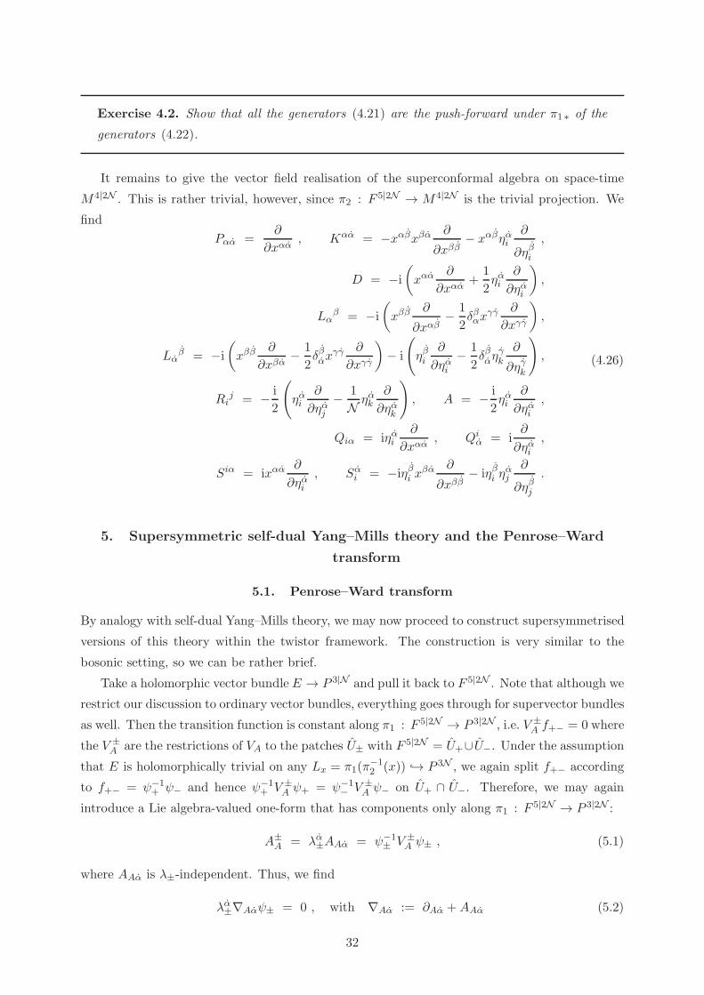
Exercise 4.2. Show that all the generators (4.21) are the push-forward under π1 ∗ of the
generators (4.22).
It remains to give the vector field realisation of the superconformal algebra on space-time
M4|2N . This is rather trivial, however, since π2 : F 5|2N → M4|2N is the trivial projection. We
find
Pαα =∂
∂xαα, Kαα = −xαβxβα ∂
∂xββ− xαβηαi
∂
∂ηβi
,
D = −i(
xαα∂
∂xαα+
1
2ηαi
∂
∂ηαi
)
,
Lαβ = −i
(
xββ∂
∂xαβ− 1
2δβαx
γγ ∂
∂xγγ
)
,
Lαβ = −i
(
xββ∂
∂xβα− 1
2δβαx
γγ ∂
∂xγγ
)
− i
(
ηβi∂
∂ηαi− 1
2δβαη
γk
∂
∂ηγk
)
,
Rij = − i
2
(
ηαi∂
∂ηαj− 1
N ηαk∂
∂ηαk
)
, A = − i
2ηαi
∂
∂ηαi,
Qiα = iηαi∂
∂xαα, Qiα = i
∂
∂ηαi,
Siα = ixαα∂
∂ηαi, Sαi = −iηβi xβα
∂
∂xββ− iηβi η
αj
∂
∂ηβj
.
(4.26)
5. Supersymmetric self-dual Yang–Mills theory and the Penrose–Ward
transform
5.1. Penrose–Ward transform
By analogy with self-dual Yang–Mills theory, we may now proceed to construct supersymmetrised
versions of this theory within the twistor framework. The construction is very similar to the
bosonic setting, so we can be rather brief.
Take a holomorphic vector bundle E → P 3|N and pull it back to F 5|2N . Note that although we
restrict our discussion to ordinary vector bundles, everything goes through for supervector bundles
as well. Then the transition function is constant along π1 : F 5|2N → P 3|2N , i.e. V ±A f+− = 0 where
the V ±A are the restrictions of VA to the patches U± with F 5|2N = U+∪U−. Under the assumption
that E is holomorphically trivial on any Lx = π1(π−12 (x)) → P 3N , we again split f+− according
to f+− = ψ−1+ ψ− and hence ψ−1
+ V ±A ψ+ = ψ−1
− V ±A ψ− on U+ ∩ U−. Therefore, we may again
introduce a Lie algebra-valued one-form that has components only along π1 : F 5|2N → P 3|2N :
A±A = λα±AAα = ψ−1
± V ±A ψ± , (5.1)
where AAα is λ±-independent. Thus, we find
λα±∇Aαψ± = 0 , with ∇Aα := ∂Aα +AAα (5.2)
32
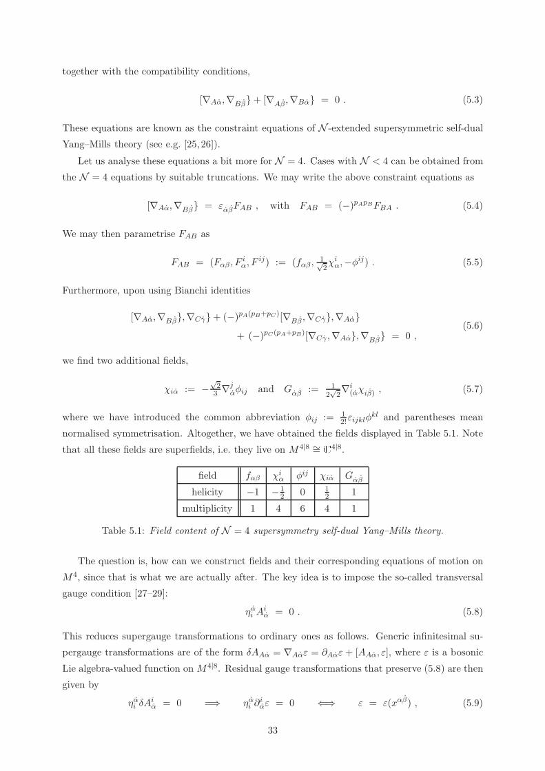
together with the compatibility conditions,
[∇Aα,∇Bβ+ [∇Aβ,∇Bα = 0 . (5.3)
These equations are known as the constraint equations of N -extended supersymmetric self-dual
Yang–Mills theory (see e.g. [25, 26]).
Let us analyse these equations a bit more for N = 4. Cases with N < 4 can be obtained from
the N = 4 equations by suitable truncations. We may write the above constraint equations as
[∇Aα,∇Bβ = εαβFAB , with FAB = (−)pApBFBA . (5.4)
We may then parametrise FAB as
FAB = (Fαβ , Fiα, F
ij) := (fαβ,1√2χiα,−φij) . (5.5)
Furthermore, upon using Bianchi identities
[∇Aα,∇Bβ,∇Cγ+ (−)pA(pB+pC)[∇Bβ ,∇Cγ,∇Aα+ (−)pC(pA+pB)[∇Cγ ,∇Aα,∇Bβ = 0 ,
(5.6)
we find two additional fields,
χiα := −√23 ∇
jαφij and Gαβ := 1
2√2∇i(αχiβ) , (5.7)
where we have introduced the common abbreviation φij := 12!εijklφ
kl and parentheses mean
normalised symmetrisation. Altogether, we have obtained the fields displayed in Table 5.1. Note
that all these fields are superfields, i.e. they live on M4|8 ∼= C4|8.
field fαβ χiα φij χiα Gαβ
helicity −1 −12 0 1
2 1
multiplicity 1 4 6 4 1
Table 5.1: Field content of N = 4 supersymmetry self-dual Yang–Mills theory.
The question is, how can we construct fields and their corresponding equations of motion on
M4, since that is what we are actually after. The key idea is to impose the so-called transversal
gauge condition [27–29]:
ηαi Aiα = 0 . (5.8)
This reduces supergauge transformations to ordinary ones as follows. Generic infinitesimal su-
pergauge transformations are of the form δAAα = ∇Aαε = ∂Aαε+ [AAα, ε], where ε is a bosonic
Lie algebra-valued function on M4|8. Residual gauge transformations that preserve (5.8) are then
given by
ηαi δAiα = 0 =⇒ ηαi ∂
iαε = 0 ⇐⇒ ε = ε(xαβ) , (5.9)
33

i.e. we are left with gauge transformations on space-time M4. Then, by defining the recursion
operator D := ηαi ∇iα = ηαi ∂iα and by using the Bianchi identities (5.6), after a somewhat lengthy
calculation we obtain the following set of recursion relations:
DAαα = − 1√2εαβη
βi χ
iα ,
(1 + D)Aiα = −εαβηβj φ
ij ,
Dφij =√2ηα[iχj]α ,
Dχiα =√2ηαj ∇ααφij ,
Dχiα = − 1√2ηβi Gαβ +
1√2εαβη
βj [φ
jk, φki] ,
DGαβ =√2ηγi εγ(α[χjβ), φ
ij ] ,
(5.10)
where, as before, parentheses mean normalised symmetrisation while the brackets denote norm-
alised anti-symmetrisation of the enclosed indices. These equations determine all superfields to
order n+ 1, provided one knows them to n-th order in the fermionic coordinates.
At this point, it is helpful to present some formulæ which simplify this argument a great deal.
Consider some generic superfield f . Its explicit η-expansion has the form
f =f +
∑
k≥1
ηγ1j1 · · · ηγkjkf j1···jkγ1···γk . (5.11)
Here and in the following, the circle refers to the zeroth-order term in the superfield expansion of
some superfield f . Furthermore, we have Df = ηγ1j1 [ ]j1γ1 , where the bracket [ ]j1γ1 is a composite
expression of some superfields. For example, we have DAαα = 1√2ηγ1j1 [αα]
j1γ1, with [αα]j1γ1 =
−εαγ1χj1α . Now let
D [ ]j1···jkγ1···γk = ηγk+1
jk+1[ ]
j1···jk+1
γ1···γk+1. (5.12)
Then we find after a successive application of D
f =f +
∑
k≥1
1
k!ηγ1j1 · · · η
γkjk
[ ]j1···jkγ1···γk . (5.13)
If the recursion relation of f is of the form (1 + D)f = ηγ1j1 [ ]j1γ1 as it happens to be for Aiα, thenf = 0 and the superfield expansion is of the form
f =∑
k≥1
k
(k + 1)!ηγ1j1 · · · η
γkjk
[ ]j1···jkγ1···γk . (5.14)
Using these expressions, one obtains the following results for the superfields Aαα and Aiα:
Aαα =Aαα + 1√
2εαβ
χiαη
βi + · · · ,
Aiα = − 12!εαβ
φ ijηβj −
√2
3! εijklεαβ
χkγη
γl η
βj +
+ 32·4!ε
ijklǫαβ(−Gγδδ
ml + εγδ[
φmn,
φnl])η
γkη
δmη
βj + · · · .
(5.15)
34
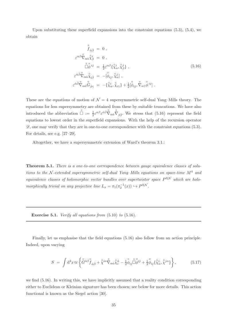
Upon substituting these superfield expansions into the constraint equations (5.3), (5.4), we
obtain
f αβ = 0 ,
εαβ∇αα
χiβ = 0 ,
φ ij = 1
2εαβχiα,
χjβ ,
εαβ∇αα
χiβ = −[
φij,
χjα] ,
εαβ∇αα
Gβγ = −χiα,
χiγ+ 1
2 [φij ,
∇αγ
φ ij] .
(5.16)
These are the equations of motion of N = 4 supersymmetric self-dual Yang–Mills theory. The
equations for less supersymmetry are obtained from these by suitable truncations. We have also
introduced the abbreviation := 1
2εαβεαβ
∇αα
∇ββ. We stress that (5.16) represent the field
equations to lowest order in the superfield expansions. With the help of the recursion operator
D , one may verify that they are in one-to-one correspondence with the constraint equations (5.3).
For details, see e.g. [27–29].
Altogether, we have a supersymmetric extension of Ward’s theorem 3.1.:
Theorem 5.1. There is a one-to-one correspondence between gauge equivalence classes of solu-
tions to the N -extended supersymmetric self-dual Yang–Mills equations on space-time M4 and
equivalence classes of holomorphic vector bundles over supertwistor space P 3|N which are holo-
morphically trivial on any projective line Lx = π1(π−12 (x)) → P 3|N .
Exercise 5.1. Verify all equations from (5.10) to (5.16).
Finally, let us emphasise that the field equations (5.16) also follow from an action principle.
Indeed, upon varying
S =
∫
d4x tr
Gαβ
f αβ +
χiα
∇αα
χαi − 1
2
φij
φij + 1
2
φij
χiα,
χjα
, (5.17)
we find (5.16). In writing this, we have implicitly assumed that a reality condition corresponding
either to Euclidean or Kleinian signature has been chosen; see below for more details. This action
functional is known as the Siegel action [30].
35

Remark 5.1. Let us briefly comment on hidden symmetry structurs of self-dual Yang–Mills
theories. Since Pohlmeyer’s work [31], it has been known that self-dual Yang–Mills theory
possess infinitely many hidden non-local symmetries. Such symmetries are accompanied
by conserved non-local charges. As was shown in [32–36, 14], these symmetries are affine
extensions of internal symmetries with an underlying Kac–Moody structure. See [37] for
a review. Subsequently, Popov & Preitschopf [38] found affine extensions of conformal
symmetries of Kac–Moody/Virasoro-type. A systematic investigation of symmetries based
on twistor and cohomology theory was performed in [39] (see also [40,41] and the text book
[1]), where all symmetries of the self-dual Yang–Mills equations were derived. In [42, 43]
(see [44] for a review), these ideas were extended to N -extended self-dual Yang–Mills theory.
For some extensions to the full N = 4 supersymmetric Yang–Mills theory, see [45]. Notice
that the symmetries of the self-dual Yang–Mills equations are intimitately connected with
one-loop maximally-helicity-violating scattering amplitudes [46–49]. See also Part II of
these lecture notes.
Exercise 5.2. Verify that the action functional (5.17) is invariant under the following
supersymmetry transformations (αi is some constant anti-commuting spinor):
δAαα = − 1√
2εαβ
βi
χiα ,
δφij =
√2α[i
χj]α ,
δχiα =
√2αj
∇αα
φij ,
δχiα = − 1√
2βi
Gαβ +
1√2εαβ
βj [
φjk,
φki] ,
δGαβ =
√2γi εγ(α[
χjβ),
φij ] .
5.2. Holomorphic Chern–Simons theory
Let us pause for a moment and summarise what we have achieved so far. In the preceding sections,
we have discussed N = 4 supersymmetric self-dual Yang–Mills theory by means of holomorphic
vector bundles E → P 3|4 over the supertwistor space P 3|4 that are holomorphically trivial on
all projective lines Lx = π1(π−12 (x)) → P 3|4. These bundles are given by holomorphic transition
functions f = f+−. We have further shown that the field equations of N = 4 supersymmetric
self-dual Yang–Mills theory arise upon varying a certain action functional on space-time, the
Siegel action. Figure 5.1. summarises pictorially our previous discussion.
The question that now arises and which is depicted in Figure 5.1. concerns the formulation
of a corresponding action principle on the supertwistor space. Certainly, such an action, if it
36

exists, should correspond to the Siegel action on space-time. However, in constructing such
a twistor space action, we immediately face a difficulty. Our above approach to the twistor
re-formulation of field theories, either linear or non-linear, is intrinsically on-shell: Holomorphic
functions on twistor space correspond to solutions to field equations on space-time and vice versa.
In particular, holomorphic transition functions of certain holomorphic vector bundles E → P 3|4
correspond to solutions to the N = 4 supersymmetric self-dual Yang–Mills equations. Therefore,
we somehow need an ‘off-shell approach’ to holomorphic vector bundles, that is, we need a theory
on supertwistor space that describes complex vector bundles such that the on-shell condition is
the holomorphicity of these bundles.
?
Siegel action
of N = 4 supersymmetric
self-dual Yang–Mills theory
holomorphic vector bundles
E → P 3|4
trivial on any Lx → P 3|4
given by f = f+−
solutions to the N = 4
supersymmetric self-dual
Yang–Mills equations
on M4
66
-
-
Figure 5.1: Correspondences between supertwistor space and space-time.
Before we delve into this issue, let us formalise our above approach to holomorphic vector
bundles (which is also known as the Cech approach). Consider a complex (super)manifold (X,O)with an open covering U = Ui. We are interested in holomorphic maps from open subsets of
X into GL(r,C) as well as in the sheaf GL(r,O) of such matrix-valued functions.14 Notice that
GL(r,O) is a non-Abelian sheaf contrary to the Abelian sheaves considered so far. A q-cochain
of the covering U with values in GL(r,O) is a collection f = fi0···iq of sections of the sheaf
GL(r,O) over non-empty intersections Ui0 ∩ · · · ∩ Uiq . We will denote the set of such q-cochains
by Cq(U,GL(r,O)). We stress that it has a group structure, where the multiplication is just
pointwise multiplication.
We may define the subsets of cocycles Zq(U,GL(r,O)) ⊂ Cq(U,GL(r,O)). For example, for
q = 0, 1 they are given by
Z0(U,GL(r,O)) := f ∈ C0(U,GL(r,O)) | fi = fj on Ui ∩ Uj 6= ∅ ,Z1(U,GL(r,O)) := f ∈ C1(U,GL(r,O)) | fij = f−1
ji on Ui ∩ Uj 6= ∅and fijfjkfki = 1 on Ui ∩ Uj ∩ Uk 6= ∅ .
(5.18)
14Basically everything we shall say below will also apply to GL(r|s,O) and hence to supervector bundles. As we
are only concerned with ordinary vector bundles (after all we are interested in SU(r) gauge theory), we will stick
to GL(r,O) for concreteness. See e.g. [44] for the following treatment in the context of supervector bundles.
37

These sets will be of particular interest. We remark that from the first of these two definitions
it follows that Z0(U,GL(r,O)) coincides with the group of global sections, H0(U,GL(r,O)), ofthe sheaf GL(r,O). Note that in general the subset Z1(U,GL(r,O)) ⊂ C1(U,GL(r,O)) is not
a subgroup of the group C1(U,GL(r,O)). For notational reasons, we shall denote elements of
C0(U,GL(r,O)) also by h = hi.We say that two cocycles f, f ′ ∈ Z1(U,GL(r,O)) are equivalent if f ′ij = h−1
i fijhj for some
h ∈ C0(U,GL(r,O)), since one can always absorb the h = hi in a re-definition of the frame
fields. Notice that this is precisely the transformation we already encountered in (3.23). The set
of equivalence classes induced by this equivalence relation is the first Cech cohomology set and de-
noted by H1(U,GL(r,O)). If the Ui are all Stein (see Remark 5.2.)—in the case of supermanifolds
X we need the body to be covered by Stein manifolds—we have the bijection
H1(U,GL(r,O)) ∼= H1(X,GL(r,O)) , (5.19)
otherwise one takes the inductive limit (see Remark 2.2.).
Remark 5.2. We call an ordinary complex manifold (X,O) Stein if X is holomorphically
convex (that is, the holomorphically convex hull of any compact subset of X is again compact
in X) and for any x, y ∈ X with x 6= y there is some f ∈ O such that f(x) 6= f(y).
To sum up, we see that within the Cech approach, rank-r holomorphic vector bundles over some
complex (super)manifold X are parametrised by H1(X,GL(r,O)). Notice that our cover U± ofthe (super)twistor space is Stein and so H1(U±,GL(r,O)) ∼= H1(P 3|N ,GL(r,O)). This in turn
explains that all of our above constructions are independent of the choice of cover.
Another approach to holomorphic vector bundles is the so-called Dolbeault approach. Let X
be a complex (super)manifold and consider a rank-r complex vector bundleE → X. Furthermore,
we let Ωp,q(X) be the smooth differential (p, q)-forms on X and ∂ : Ωp,q(X)→ Ωp,q+1(X) be the
anti-holomorphic exterior derivative. A (0, 1)-connection on E is defined by a covariant differential
∇0,1 : Ωp,q(X,E) → Ωp,q+1(X,E) which satisfies the Leibniz formula. Here, Ωp,q(X,E) :=
Ωp,q(X) ⊗ E. Locally, it is of the form ∇0,1 = ∂ + A0,1, where A0,1 is a differential (0, 1)-form
with values in EndE which we shall refer to as the connection (0, 1)-form. The complex vector
bundle E is said to be holomorphic if the (0, 1)-connection is flat, that is, if the corresponding
curvature vanishes,
F 0,2 = (∇0,1)2 = ∂A0,1 +A0,1 ∧A0,1 = 0 . (5.20)
In other words, ∇0,1 defines a holomorphic structure on E. The group H0(X,GL(r,S)), where Sis the sheaf of smooth functions on X, acts on A0,1 by gauge transformations,
A0,1 7→ g−1A0,1g + g−1∂g , with g ∈ H0(X,GL(r,S)) . (5.21)
Clearly, such transformations leave (5.20) invariant, hence they do not change the holomorphic
structure on E. Therefore, two solutions to F 0,2 = 0 are regarded as equivalent if they dif-
fer by such a gauge transformation. We shall then denote the space of equivalence classes by
H0,1∇0,1(X,E).
38
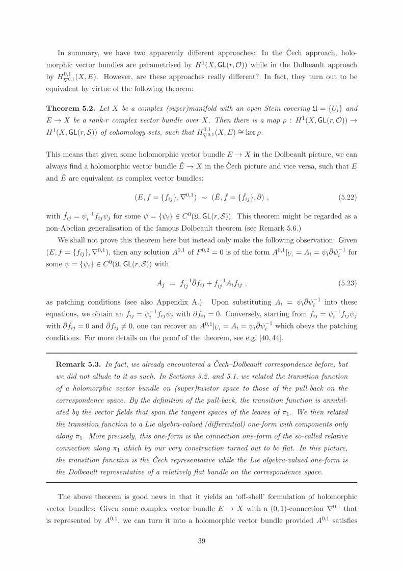
In summary, we have two apparently different approaches: In the Cech approach, holo-
morphic vector bundles are parametrised by H1(X,GL(r,O)) while in the Dolbeault approach
by H0,1∇0,1(X,E). However, are these approaches really different? In fact, they turn out to be
equivalent by virtue of the following theorem:
Theorem 5.2. Let X be a complex (super)manifold with an open Stein covering U = Ui and
E → X be a rank-r complex vector bundle over X. Then there is a map ρ : H1(X,GL(r,O)) →H1(X,GL(r,S)) of cohomology sets, such that H0,1
∇0,1(X,E) ∼= ker ρ.
This means that given some holomorphic vector bundle E → X in the Dolbeault picture, we can
always find a holomorphic vector bundle E → X in the Cech picture and vice versa, such that E
and E are equivalent as complex vector bundles:
(E, f = fij,∇0,1) ∼ (E, f = fij, ∂) , (5.22)
with fij = ψ−1i fijψj for some ψ = ψi ∈ C0(U,GL(r,S)). This theorem might be regarded as a
non-Abelian generalisation of the famous Dolbeault theorem (see Remark 5.6.)
We shall not prove this theorem here but instead only make the following observation: Given
(E, f = fij,∇0,1), then any solution A0,1 of F 0,2 = 0 is of the form A0,1|Ui= Ai = ψi∂ψ
−1i for
some ψ = ψi ∈ C0(U,GL(r,S)) with
Aj = f−1ij ∂fij + f−1
ij Aifij , (5.23)
as patching conditions (see also Appendix A.). Upon substituting Ai = ψi∂ψ−1i into these
equations, we obtain an fij = ψ−1i fijψj with ∂fij = 0. Conversely, starting from fij = ψ−1
i fijψj
with ∂fij = 0 and ∂fij 6= 0, one can recover an A0,1|Ui= Ai = ψi∂ψ
−1i which obeys the patching
conditions. For more details on the proof of the theorem, see e.g. [40, 44].
Remark 5.3. In fact, we already encountered a Cech–Dolbeault correspondence before, but
we did not allude to it as such. In Sections 3.2. and 5.1. we related the transition function
of a holomorphic vector bundle on (super)twistor space to those of the pull-back on the
correspondence space. By the definition of the pull-back, the transition function is annihil-
ated by the vector fields that span the tangent spaces of the leaves of π1. We then related
the transition function to a Lie algebra-valued (differential) one-form with components only
along π1. More precisely, this one-form is the connection one-form of the so-called relative
connection along π1 which by our very construction turned out to be flat. In this picture,
the transition function is the Cech representative while the Lie algebra-valued one-form is
the Dolbeault representative of a relatively flat bundle on the correspondence space.
The above theorem is good news in that it yields an ‘off-shell’ formulation of holomorphic
vector bundles: Given some complex vector bundle E → X with a (0, 1)-connection ∇0,1 that
is represented by A0,1, we can turn it into a holomorphic vector bundle provided A0,1 satisfies
39

the ‘on-shell condition’ (5.20). The latter equation is also known as the equation of motion of
holomorphic Chern–Simons theory. What about an action? Is it possible to write down an action
functional which yields F 0,2 = 0. The answer is yes, but not always. The action that gives
F 0,2 = 0 is [50]
S = − 1
2πi
∫
XΩ ∧ tr
A0,1 ∧ ∂A0,1 + 2
3A0,1 ∧A0,1 ∧A0,1
︸ ︷︷ ︸
=: ω
= − 1
2πi
∫
XΩ ∧ ω , (5.24)
where the pre-factor has been chosen for later convenience. A few words are in order. For a
moment, let us assume that X is an ordinary complex manifold. The holomorphic Chern–Simons
form
ω = trA0,1 ∧ ∂A0,1 + 2
3A0,1 ∧A0,1 ∧A0,1
(5.25)
is a (0, 3)-form on X. Furthermore, the action (5.24) is invariant under (5.21) provided Ω is
holomorphic (and g is homotopic to the identity and g → 1 asymptotically). Thus, dimCX = 3
and so Ω is a holomorphic (3, 0)-form. In addition, Ω should be globally defined, since the Chern–
Simons form is. This in turn puts severe restrictions on the geometric properties of X. Complex
manifolds that admit such forms are called formal Calabi–Yau manifolds. The name is chosen
to distinguish them from ‘honest’ Calabi–Yau manifolds which are (compact) complex manifolds
that are Kahler and that admit globally defined holomorphic top-forms.15 Equivalently, we could
say that the canonical bundle K := detT ∗ 1,0X is trivial, since Ω is a section of K. Notice that
sections of K are also called holomorphic volume forms. Therefore, while the equation F 0,2 = 0
makes sense on any complex manifold X, the corresponding action functional is defined only for
three-dimensional formal Calabi–Yau manifolds.
Let us take a closer look at the twistor space P 3. Certainly, it is a three-dimensional complex
manifold. But does it admit a globally defined holomorphic volume form Ω0? In fact it does not,
since
Ω0 = 14dz
α ∧ dzα ∧ dλβλβ , (5.26)
which shows that K ∼= O(−4) which is not a trivial bundle. Therefore, it is not possible to
write down an action principle for holomorphic Chern–Simons theory on P 3. However, somehow
we could have expected that as we do not have an action on space-time either (apart from the
Lagrange multiplier type action∫d4xGαβfαβ with the additional field Gαβ; see Section 6.1. for
more details).
But what about N = 4 supersymmetric self-dual Yang–Mills theory? We know that there is
an action principle. The holomorphic volume form Ω on supertwistor space P 3|4 is given by
Ω = Ω0 ⊗ Ω1 , with Ω1 := 14!ε
ijkldηidηjdηkdηl , (5.27)
where Ω0 is as above. To determine whether this is globally defined or not, we have to take into
account the definition of the Berezin integral over fermionic coordinates:∫
dηi ηj = δij . (5.28)
15For a beautiful recent exposition on Calabi–Yau manifolds, see e.g. the lecture notes [51].
40

If one re-scales ηi 7→ t ηi, with t ∈ C \ 0, then dηi 7→ t−1dηi. Therefore, the dηi transform
oppositely to ηi and thus they are not differential forms. In fact, they are so-called integral forms.
This shows that (5.27) is indeed globally defined, since Ω0 is a basis section of O(−4) while Ω1
is a basis section of O(4) and so Ω is of homogeneity zero since O(−4) ⊗O(4) ∼= O. Hence, the
Berezinian line bundle Ber (which is the supersymmetric generalisation of the canonical bundle) of
the supertwistor space P 3|4 is trivial. In this sense, P 3|4 is a formal Calabi–Yau supermanifold.16
In Remark 5.4., we show that any three-dimensional complex spin manifold can be associated
with a formal Calabi–Yau supermanifold via the LeBrun construction [60]. Notice that if we
had instead considered P 3|N , then Ω would have been of homogeneity N − 4. Altogether, we
see that the holomorphic Chern–Simons action (5.24) can only be written down for N = 4. In
this case, the symmetry group that preserves the holomorphic measure Ω is PSL(4|4,C). This isthe complexification of the N = 4 superconformal group in four dimensions (which is the global
symmetry group of N = 4 supersymmetric Yang–Mills theory). See also Section 4.3.
We are almost done. We just need to clarify one issue. The connection one-form A0,1 is
an ‘honest’ differential form, i.e. it is not an integral form like Ω1. However, in general A0,1
also depends on ηi and furthermore on the differential (0, 1)-forms dηi. As there is no way of
integrating fermionic differential forms, the integral (5.24) seems not to make sense. However,
this is not the case since the supertwistor space P 3|4 can be regarded as a holomorphic vector
bundle over the twistor space P 3; see Exercise 4.1. and Equation (4.11). Hence, there always
exists a gauge in which∂
∂ηiyA0,1 = 0 and
∂
∂ηiy ∂A0,1 = 0 , (5.29)
since the fibres P 3|4 → P 3 do not have sufficient non-trivial topology. Thus, in this gauge A0,1
only has a holomorphic dependence on ηi. We shall refer to this gauge as Witten gauge [53].
Summarising our above discussion, we have found an action principle on supertwistor space
for holomorphic vector bundles in the case of N = 4 supersymmetry.17 Therefore, the missing
box in Figure 5.1. can be filled in with the help of (5.24). In the remainder of this section, we
demonstrate explicitly that (5.24) indeed implies (5.17) on space-time. Our discussion below is
based on [53,65–67].
For concreteness, let us choose reality conditions that lead to a Euclidean signature real slice
in M4. At the end of Section 3.2., we saw that they arise from an anti-holomorphic involution
on P 3. Similarly, we may introduce an anti-holomorphic involution τ : P 3|4 → P 3|4 leading to
Euclidean superspace. In particular,
τ(zA, λα) := (zA, λα) := (zBCBA, Cα
βλβ) , (5.30)
16In fact, P 3|4 is also an ‘honest’ Calabi–Yau space in the sense of being Kahler and admitting a super Ricci-flat
metric [52, 53]. Note that for ordinary manifolds, the Kahler condition together with the existence of a globally
defined holomorphic volume form always implies the existence of a Ricci-flat metric. This is the famous Yau
theorem. However, an analog of Yau’s theorem in the context of supermanifolds does not exist. See e.g. [52,54–59].17An analogous action has been found by Sokatchev [61] in the harmonic superspace approach. Recently, Popov
gave alternative twistor space action principles in [62]. Interestingly, similar actions also exist for maximal N = 8
self-dual supergravity in the harmonic space approach [63] as well as in the twistor approach [64].
41
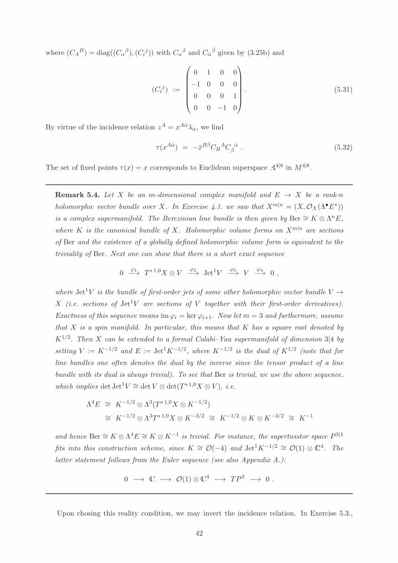
where (CAB) = diag((Cα
β), (Cij)) with Cα
β and Cαβ given by (3.25b) and
(Cij) :=
0 1 0 0
−1 0 0 0
0 0 0 1
0 0 −1 0
. (5.31)
By virtue of the incidence relation zA = xAαλα, we find
τ(xAα) = −xBβCBACβ α . (5.32)
The set of fixed points τ(x) = x corresponds to Euclidean superspace R4|8 in M4|8.
Remark 5.4. Let X be an m-dimensional complex manifold and E → X be a rank-n
holomorphic vector bundle over X. In Exercise 4.1. we saw that Xm|n = (X,OX (Λ•E∗))
is a complex supermanifold. The Berezinian line bundle is then given by Ber ∼= K ⊗ ΛnE,
where K is the canonical bundle of X. Holomorphic volume forms on Xm|n are sections
of Ber and the existence of a globally defined holomorphic volume form is equivalent to the
triviality of Ber. Next one can show that there is a short exact sequence
0ϕ1−→ T ∗ 1,0X ⊗ V ϕ2−→ Jet1V
ϕ3−→ Vϕ4−→ 0 ,
where Jet1V is the bundle of first-order jets of some other holomorphic vector bundle V →X (i.e. sections of Jet1V are sections of V together with their first-order derivatives).
Exactness of this sequence means imϕi = kerϕi+1. Now let m = 3 and furthermore, assume
that X is a spin manifold. In particular, this means that K has a square root denoted by
K1/2. Then X can be extended to a formal Calabi–Yau supermanifold of dimension 3|4 by
setting V := K−1/2 and E := Jet1K−1/2, where K−1/2 is the dual of K1/2 (note that for
line bundles one often denotes the dual by the inverse since the tensor product of a line
bundle with its dual is always trivial). To see that Ber is trivial, we use the above sequence,
which implies det Jet1V ∼= detV ⊗ det(T ∗ 1,0X ⊗ V ), i.e.
Λ4E ∼= K−1/2 ⊗ Λ3(T ∗ 1,0X ⊗K−1/2)
∼= K−1/2 ⊗ Λ3T ∗ 1,0X ⊗K−3/2 ∼= K−1/2 ⊗K ⊗K−3/2 ∼= K−1
and hence Ber ∼= K ⊗Λ4E ∼= K ⊗K−1 is trivial. For instance, the supertwistor space P 3|4
fits into this construction scheme, since K ∼= O(−4) and Jet1K−1/2 ∼= O(1) ⊗ C4. The
latter statement follows from the Euler sequence (see also Appendix A.):
0 −→ C −→ O(1)⊗C4 −→ TP 3 −→ 0 .
Upon chosing this reality condition, we may invert the incidence relation. In Exercise 5.3.,
42
you will derive the following result:
xAα =zAλα − zAλα
λαλα. (5.33)
This shows that as real manifolds, we have the following diffeomorphisms:
P 3|4 ∼= R4|8 ×CP 1 ∼= R4|8 × S2 , (5.34)
and hence we have a non-holomorphic fibration
π : P 3|4 → R4|8 ,
(zA, λα) 7→ xAα =zAλα − zAλα
λαλα.
(5.35)
The same holds true for P 3|N ∼= R4|2N ×CP 1 ∼= R4|2N × S2. Therefore, in the real setting we
may alternatively work with this single fibration instead of the double fibration (4.15) and we
shall do so in the following. This will be most convenient for our purposes.
Exercise 5.3. Verify (5.33).
In order to write down the ∂-operator on P 3|4, we need a basis for differential (0, 1)-forms and
(0, 1)-vector fields in the non-holomorphic coordinates (xAα, λα). Using the conventions
∂
∂λαλβ = δα
β,
∂
∂λαydλβ = δα
β,
∂
∂λαλβ = δα
β,
∂
∂λαydλβ = δα
β(5.36a)
and∂
∂xAαxBβ = δBA δ
βα ,
∂
∂xAαydxBβ = δBA δ
βα , (5.36b)
we have
e0 =[dλλ]
[λλ]2and eA = −dxAαλα
[λλ], (5.37a)
where [ρλ] := εαβραλβ = ραλα, e.g. [dλλ] = dλαλ
α, together with
V0 = [λλ]λα∂
∂λαand VA = λα∂Aα . (5.37b)
In this sense, V0ye0 = 1, VAye
B = δBA , V0yeA = 0 and VAye
0 = 0 and the ∂-operator is ∂ =
e0V0 + eAVA. Notice that the vector fields (4.14) are (0, 1)-vector fields in this real setting. The
holomorphic volume form (5.27) takes the form
Ω = Ω0 ⊗ Ω1
= 14 [λλ]
4e0 ∧ eα ∧ eα ⊗ Ω1 = 14 [dλλ] ∧ εαβλαλβdxαα ∧ dxββ ⊗ Ω1 ,
(5.38)
where Ω1 is given in (5.27). Here, we do not re-write the dηi (or rather the corresponding integral
forms) in terms of the ei. The reason for this becomes transparent in our subsequent discussion.
43
Note also that the e0, eA are obtained from (5.37a) via complex conjugation (or equivalently, via
the involution τ).
Working in Witten gauge (5.29), we have
A0,1 = e0A0 + eαAα , (5.39)
where A0 and Aα have a holomorphic dependence on ηi. In particular, we may expand A0,1
according to
A0,1 =A+ ηi
χi + 1
2!ηiηjφij + 1
3!ηiηjηkεijkl χ
l+ 1
4!ηiηjηkηlεijkl
G , (5.40)
where the coefficientsA,
χi,
φij ,
χland
G are differential (0, 1)-forms of homogeneity 0, −1, −2,
−3 and −4 that depend only on x, λ and λ.
At this stage, it is useful to digress a bit by discussing the linearised equations of motion.
At the linearised level, (5.20) reads as ∂A0,1 = 0 and the gauge transformations (5.21) reduce
to A0,1 7→ ∂ε. Therefore, the coefficient fields of (5.40) represent Lie algebra-valued elements
of the Dolbeault cohomology group H0,1
∂(P 3,O(−2h − 2)) for h = −1, . . . , 1. By the Dolbeault
theorem, we have H0,1∂
(P 3,O(−2h−2)) ∼= H1(P 3,O(−2h−2)); see Remark 5.6. for more details.
Therefore, we can apply Theorem 2.2. to conclude that on space-time, these fields correspond tofαβ ,
χiα,
φij ,
χiα and
Gαβ which is precisely the field content displayed in Table 5.1. Hence, one
superfield A0,1 on supertwistor space P 3|4 encodes the whole particle spectrum of N = 4 self-dual
supersymmetric Yang–Mills theory.
As a next step, we need to remove the extra gauge symmetry beyond the space-time gauge
transformations (after all we want to derive the Siegel action). To achieve this, we have to further
gauge-fix A0,1 (on top of the already imposed Witten gauge). This procedure is in spirit of our
discussion in Section 5.1., where we have shown how to go from the constraint equations of
supersymmetric self-dual Yang–Mills theory to its actual field equations. To this end, we impose
a gauge called space-time gauge [65,67,68]
∂†L(e0A0) = 0 , (5.41)
on all fibres of (5.35). Here, e0A0 is understood as the restriction of A0,1 to the projective line
Lx → P 3|4 and ∂†L = −∗∂L∗ is the adjoint of ∂L on Lx. This amounts to choosing a metric
on Lx which we take to be the Fubini–Study metric (see also Remark 5.5.). Put differently, we
require e0A0 to be fibrewise co-closed with respect to the Fubini–Study metric on each Lx ∼= CP 1.
Residual gauge transformations that preserve (5.41) are then given by those g ∈ H0(P 3|4,GL(r,S))that obey
∂†L∂Lg = 0 , (5.42)
as one may straightforwardly check by inspecting (5.21). If we let (·, ·) be a metric on the space
of matrix-valued differential forms on each Lx, then 0 = (g, ∂†L∂Lg) = (∂Lg, ∂Lg) ≥ 0. Hence,
∂Lg = 0 and so g is holomorphic on each fibre Lx and thus it must be constant (since the Lx are
compact). Altogether, g = g(xαβ) and the residual gauge freedom is precisely space-time gauge
transformations.
44

Remark 5.5. Consider CP 1 with the canonical cover U± as in Remark 1.2. In homo-
geneous coordinates λα, the Fubini–Study metric is given by
ds2 =[dλλ][dλλ]
[λλ]2
while in affine coordinates λ± we have
ds2|U± =dλ±dλ±
(1 + λ±λ±)2, with ds2|U+ = ds2|U− .
Here, λα was defined in (5.30). Notice that the Fubini–Study metric is the Kahler metric
on CP 1 with the Kahler form
K = K(λ) =[dλλ] ∧ [dλλ]
[λλ]2.
Since A0,1 is holomorphic in ηi, the gauge fixing condition ∂†L(e0A0) = 0 has to hold for each
component,
e0A0 = e0A0 + ηie
0 χi0 +
12!ηiηj e
0φij0 + 1
3!ηiηjηkεijkle0
χl0+ 1
4!ηiηjηkηlεijkle0
G0 , (5.43)
i.e.
∂†L(e0A0) = ∂†L(e
0 χi0) = ∂†L(e
0φij0 ) = ∂†L(e
0 χi0) = ∂†L(e
0G0) = 0 . (5.44)
Remark 5.6. Let X be a complex manifold and E → X be a holomorphic vector
bundle. Furthermore, we denote the ∂-harmonic (p, q)-forms on X with values in E by
Harmp,q∂
(X,E), where ∂ is the anti-holomorphic exterior derivative. These are forms
ω ∈ Harmp,q∂
(X,E) that obey ∂ω = 0 = ∂†ω. In addition, let Hp,q∂
(X,E) be the ∂-
cohomology groups with coefficients in E, i.e. elements of Hp,q∂
(X,E) are ∂-closed E-valued
(p, q)-forms which are not ∂-exact. If X is compact, the Hodge theorem establishes the
following isomorphism:
Harmp,q∂
(X,E) ∼= Hp,q∂
(X,E) .
The Dolbeault theorem establishes another isomorphism for X not necessarily compact
Hp,q∂
(X,E) ∼= Hq(X,ΛpT ∗X ⊗ E) ,
where Hq(X,ΛpT ∗X⊗E) is the q-th Cech cohomology group with coefficients in ΛpT ∗X⊗E.
For details, see e.g. [9, 69].
Notice that e0A0, e
0 χ i0, e
0φ ij0 , e
0 χi0, and e0
G0 take values in O(m) ⊗ EndE with m being
0, . . . ,−4. Furthermore, e0A0 is also ∂L-closed since dimC Lx = 1 and therefore it is harmonic
along the fibres. Likewise, all the component fields of e0A0 are fibrewise harmonic. Therefore,
45

the Hodge and Dolbeault theorems (see Remark 5.6.) then tell us that the restriction of these
components to the fibres are EndE-valued elements of H1(CP 1,O(−2h − 2)) since Lx ∼= CP 1.
From Table 2.2, we conclude that H1(CP 1,O(−2h−2)) = 0 for h = −1,−12 and hence
A0 =
χi0 =
0. Furthermore, H1(CP 1,O(−2h − 2)) ∼= C2h+1 for h ≥ 0 and therefore, the other components
may be taken as (see also [70]):
A = e0
A0 + eα
Aα = eα
Aα ,
χi = e0
χi0 + eα
χiα = eα
χiα ,
φij = e0
φij0 + eα
φijα = e0
φij + eα
φijα ,
χi= e0
χi0+ eα
χiα
= 2e0χiαλ
α
[λλ]+ eα
χiα,
G = e0
G0 + eα
Gα = 3e0
Gαβλ
αλβ
[λλ]2+ eα
Gα .
(5.45)
Here, the fieldsφ ij,
χiα and
Gαβ depend only on the space-time coordinates xαβ while the
remaining fields still may depend on λα and λα. Notice that we useφij = 1
2εijkl
φkl
and similarly
for its components.
The non-trivial step in writing (5.45) is in settingA0 = 0 (and
χi0 = 0 by supersymmetry).
This implies that E is holomorphically trivial on any Lx → P 3|4, which is one of the assumptions
in Ward’s theorem; see Theorems 3.1. and 5.1. Notice that this is not guaranteed in general, but
will follow from the smallness assumption ofA0 in a perturbative context.
In terms of the expansions (5.45), the action (5.24) reads
S = − 1
2πi
∫Ω0 ∧ Ω0
[λλ]4tr
Gαβλ
αλβ
[λλ]2
(
−λγ∂αγAα + 1
2
[ Aα,
Aα
])
+
χiαλ
α
[λλ]
(
λβ∂αβχiα +
[ Aα,
χiα])
− 12
φij
(
λβ∂αβφijα +
[ Aα,
φijα
])
+ 12
φij
χiα,
χjα+
( GαV0
Aα −
χiαV0
χiα + 1
4
φijαV0
φijα
)
.
(5.46)
Note that in actual fact one should also add a gauge-fixing term and a ghost term. However,
the ghost-matter interaction is such that the Fadeev–Popov determinant is independent of A0,1.
See [67] for more details. For the time being, we therefore omit these pieces.
The fieldsGα and
χiα
appear only linearly, so they are in fact Lagrange multiplier fields.
Integrating them out enforces
V0Aα = 0 and V0
χiα = 0 (5.47)
46
and soAα and
χiα must be holomorphic in λα. Hence,
Aα = λβ
Aαβ and
χiα =
χiα (5.48)
since they are of homogeneity 1 and 0, respectively. Here,Aαβ and
χ iα depend only on xαβ.
Likewise,φijα can be eliminated as it appears only quadratically with a constant coefficient.18 We
have
V0φijα = λβ
(
∂αβφij +
[ Aαβ ,
φij])
(5.49)
which yields
φijα =
1
[λλ]λβ
∇αβ
φij , with
∇αβ := ∂αβ +
Aαβ . (5.50)
Inserting (5.48) and (5.50) into (5.46), we find
S = − 1
2πi
∫Ω0 ∧ Ω0
[λλ]4tr
Gαβ
f γδ
λαλβλγλδ
[λλ]2+
χiα
∇βγ
χiβ
λαλγ
[λλ]
+ 14
φij
∇αβ
∇αγ
φij
λαλγ
[λλ]+ 1
2
φij
χiα,
χjα
,
(5.51)
wheref αβ is the anti-self-dual part of the curvature of
Aαβ (see also (3.21)). Using
Ω0 ∧ Ω0
[λλ]4= d4x
[dλλ][dλλ]
[λλ]2(5.52)
together with the formula derived in Exercise 5.4., we can integrate out the fibres to finally arrive
at
S =
∫
d4x tr
Gαβ
f αβ +
χiα
∇αα
χαi − 1
2
φij
φij + 1
2
φij
χiα,
χjα
. (5.53)
This is nothing but the Siegel action (5.17).
Altogether, the holomorphic Chern–Simons action (5.24) on supertwistor space P 3|4 corres-
ponds to the Siegel action (5.17) on space-time. This concludes Figure 5.1. and our discussion
about N = 4 supersymmetric self-dual Yang–Mills theory.19
18Notice that if one integrates out generic quadratic pieces in the path integral, then one picks up field-dependent
functional determinants. However, in our case the ‘φ2-piece’ has a constant coefficient and hence, the determinant
is constant and thus can be absorbed in the normalisation of the path integral measure.19For twistor constructions including action functionals of other gauge field theories, see [71,57,72–76,67,68,77].
47

Exercise 5.4. Verify (5.52). Furthermore, prove that
− 1
2πi
∫
K fα1···αmgβ1···βm λβ1 · · · λβmλ
α1 · · · λαm
[λλ]m=
1
m+ 1fα1···αmg
α1···αm ,
where K is the Kahler form given in Remark 5.5. and gα1···αm and fα1···αm do not depend
on λ and λ. In fact, this is the Dolbeault version of Serre duality discussed in Remark
2.1. (see also Remark 5.6.):
H0,0∂
(CP 1,O(m)) ∼= H0,1∂
(CP 1,O(−m− 2))∗ .
More concretely, g = gα1···αmλα1 . . . λαm represents an element of H0,0∂
(CP 1,O(m)) ∼=H0(CP 1,O(m)) while
f = (m+ 1)fα1···αm
λα1 · · · λαm
[λλ]m[dλλ]
[λλ]2
is an element of H0,1∂
(CP 1,O(−m − 2)) ∼= H1(CP 1,O(−m − 2)). Here, we have used
(5.37a). Then the Dolbeault version of the pairing (2.15) is given by
(f, g) = − 1
2πi
∫
[dλλ] ∧ fg = fα1···αmgα1···αm ,
which is nothing but the above formula.
6. N = 4 supersymmetric Yang–Mills theory from supertwistor space
6.1. Motivation
So far, we have shown how N = 4 supersymmetric self-dual Yang–Mills theory can be understood
in terms of twistor geometry. The field content of this theory is displayed in Table 5.1. and the
corresponding action in (5.17). In fact, the full N = 4 supersymmetric Yang–Mills theory has
precisely the same field content but it differs in the interaction terms. The action is given by
S =
∫
d4x tr
f αβ
f αβ +
fαβ
fαβ +
φij
φij − 2
χiα
∇αα
χαi
−φij
χiα,
χjα −
φijχiα,
χαj + 1
8 [φij,
φkl][
φij ,
φkl]
.
(6.1)
By comparing the Siegel action (5.53) with the action (6.1), we realise that the Siegel action
provides only parts of the interaction terms. What about the other terms? Can they also be
understood in terms of twistors?
Before delving into this, let us first consider purely bosonic self-dual Yang–Mills theory. This
theory may be described by the action
S =
∫
tr(G ∧ F−) , (6.2)
48
since the corresponding field equations are
F− = 0 and ∇∗G = 0 . (6.3)
Hence, we obtain the self-dual Yang–Mills equations plus an equation for an anti-self-dual field G
propagating in the self-dual background. Notice that G is nothing but the field Gαβ we already
encountered. Let us modify the above action by adding the term [53]
Sε = −12ε
∫
tr(G ∧G) , with Stot = S + Sε (6.4)
where ε is some small parameter. Upon integrating out the field G, we find
Stot = 12ε
∫
tr(F− ∧ F−) = − 14ε
∫
tr(F ∧ ∗F ) + 14ε
∫
tr(F ∧ F ) , (6.5)
where we have used F− = 12(F − ∗F ). Hence, we obtain the Yang–Mills action (3.2) plus a
term proportional to the topological charge (3.7), provided we identify ε with the Yang–Mills
coupling constant g2YM. Therefore, small ε corresponds to small gYM. As we are about to study
perturbation theory, the topological term will not play a role and we may therefore work with
(6.4). Consequently, we may re-phrase our question: Can we derive∫tr(G ∧ G) or rather its
N = 4 supersymmetric extension from twistor space? This will be answered in the next section.
Exercise 6.1. Show that the action (6.1) is invariant under the following supersymmetry
transformations (iα and αi are constant anti-commuting spinors):
δAαα = −εαβiβ
χiα + εαβ
βi
χiα ,
δφij = εijkl
kα χlα − 2α[i
χj]α ,
δχiα = −2iβ
fαβ + εαβ
jβ[φik,
φjk]− 2αj
∇αα
φij ,
δχiα = 2jα
∇αα
φij + 2βi
f αβ + εαβ
βj [
φjk,
φik] .
6.2. N = 4 supersymmetric Yang–Mills theory from supertwistor space
In parts, the following discussion follows the lines of [66,67]. To obtain the full N = 4 supersym-
metric Yang–Mills action, one considers the following modification:
Stot = S + Sε , (6.6a)
where S is the holomorphic Chern–Simons action (5.24) and Sε is given by [67]
Sε = −ε∫
d4|8x log det∇0,1|Lx . (6.6b)
One takes the (0, 1)-connection ∇0,1, restricts it to the fibre Lx → P 3|4, constructs the determ-
inant of this operator and finally integrates the logarithm of this determinant over x ∈ M4|8
49

parametrising Lx ∼= CP 1. Here, we have used the common abbreviation d4|8x := d4xd8η. Note
that the action (6.6b) is invariant under the gauge transformations (5.21). This will be verified in
Exercise 6.2. Before showing that Sε really gives the missing interactions, let us emphasise that
all the constructions presented in the preceding section also apply to the full twistor space action
(6.6a) without alteration. We may therefore stick to Sε for the remainder of this section.
Exercise 6.2. Argue that the action (6.6b) is invariant under the gauge transformations
(5.21). You might find it useful to know that the determinant det∇0,1|Lx behaves under
infinitesimal gauge transformations δA0,1 = ∇0,1ε, with ε being an infinitesimal gauge
parameter, as
δ det∇0,1|Lx =
(1
2π
∫
Lx
tr(A0,1 ∧ ∂ε))
det∇0,1|Lx .
This formula is, in fact, the so-called chiral anomaly with ∇0,1 on Lx being the chiral Dirac
operator. From a physical point of view, it can best be understood in a path integral language.
If we consider two fermionic fields α and β of homogeneity −1 on Lx taking values in E|Lx
and E∗|Lx respectively with the action
Sβα =
∫
Lx
[dλλ] ∧ β∇0,1α ,
then
det∇0,1|Lx = e−W [A0,1] =
∫
DαDβ exp
(
−∫
Lx
[dλλ] ∧ β∇0,1α
)
,
where W [A0,1] is the effective action. The above formula of the gauge variation of the
determinant arises by studying variations A0,1 7→ A0,1 + δA0,1 = A0,1 + ∇0,1ε of the path
integral. See e.g. [69,78] for more details.
In what follows, we shall need the Green function of the ∂-operator on CP 1 and so it will be
useful to recapitulate some of its properties first. To this end, notice that any differential (0, 1)-
form on CP 1 is automatically ∂-closed since dimCCP 1 = 1. Furthermore, the Dolbeault cohomo-
logy groups H0,1∂
(CP 1,O(m)) vanish for m ≥ −1 since H0,1∂
(CP 1,O(m)) ∼= H1(CP 1,O(m)) and
the Cech cohomology groups H1(CP 1,O(m)) are given in Table 2.2. Therefore, any differential
(0, 1)-form ω of homogeneity m ≥ −1 is necessarily ∂-exact, i.e. ω = ∂ρ for some ρ of homo-
geneity m. We shall denote the element ρ by ∂−1ω, in the following. Again from Table 2.2., we
conclude that ∂−1ω is not unique for m ≥ 0 as one can always add a global holomorphic function
α of homogeneity m: ∂(∂−1ω + α) = ω. For m = −1, however, there are no global holomorphic
functions and so ∂−1ω is unique. Explicitly, we have
∂−1ω(λ) = − 1
2πi
∫[dλ′λ′][λλ′]
∧ ω(λ′) . (6.7)
In deriving this result, one makes use of the basis (5.37)
ω(λ) = e0ω0(λα, λα) =[dλλ]
[λλ]2ω0(λα, λα) (6.8)
50

together with
∂(λ)1
[λλ′]= 2π[dλλ]
[ξλ′]
[ξλ]δ(2)([λλ′], [λλ′]) . (6.9a)
Here, ξα is some constant spinor. The complex delta function is given by
δ(2)([λλ′], [λλ′]) := 12δ(Re[λλ′])δ(Im[λλ′]) (6.9b)
and obeys δ(2)(t[λλ′], t[λλ′]) = (tt)−1δ(2)([λλ′], [λλ′]) for t ∈ C \ 0. On support of the delta
function, λα ∝ λ′α and therefore the expression (6.9a) is independent of the choice of ξα. Notice
that ω0(tλα, tλα) = tω0(λα, λα) for t ∈ C \ 0 since ω is of homogeneity −1. Notice also that
one often writes
G(λ, λ′) := − 1
2πi [λλ′]=⇒ ∂−1ω(λ) =
∫
K(λ′)G(λ, λ′)ω0(λ′) , (6.10)
where G(λ, λ′) is referred to as the Green function of the ∂-operator or equivalently, as the integral
kernel of ∂−1-operator. Furthermore, K(λ) is the Kahler form introduced in Remark 5.5. and
ω0(λ) is short-hand notation for ω0(λα, λα).
Exercise 6.3. Verify (6.9a). You may find it useful to consider (ε ∈ R)
∂(λ)[λλ′]
[λλ′][λλ′] + ε2
in the limit ε→ 0.
After this digression, let us come back to the action Sε. To compute its space-time form, we
recall the identity
log det∇0,1|Lx = tr log∇0,1|Lx (6.11)
and consider the following power series expansion:
tr log∇0,1|Lx = tr log(∂ +A0,1)|Lx
= tr[log ∂|Lx + log(1 + ∂−1A0,1)|Lx
]
= tr
[
log ∂|Lx +
∞∑
r=1
(−1)rr
∫
Lx
r∏
s=1
K(λs)G(λs−1, λs)A0(λs)
]
, (6.12)
with the identification λ0 ≡ λr. Here, we have inserted the Green function (6.10). In addition,
we used (5.39), i.e. each A0 is the e0-coefficient of A0,1 = e0A0 + eαAα and restricted to lie on a
copy of the fibre over the same point x ∈ M4|8, i.e. λs ∈ Lx → P 3|4 for all s. Notice that A0 is
of homogeneity 2 as follows from the scaling behaviour of e0.
Adopting the gauge (5.41), we see that the series (6.12) terminates after the fourth term, since
in this gauge A0 starts only at second-order in the ηi-expansion (compare (5.40) with (5.45)). In
addition, we eventually integrate over d4|8x, so we only need to keep terms that contain all ηαi .
51

In this respect, recall that on Lx we have ηi = ηαi λα. Then there are only three types of relevant
terms: Firstly, we have theGαβ
Gαβ-term which is
− ε∫
d4|8x1
2
(3
2πi
)2 ∫
Lx
2∏
s=1
K(λs)
[λs−1λs]
× tr
1
4!εijklη1iη1jη1kη1l
Gαβλ
α1 λ
β1
[λ1λ1]21
4!εijklη2iη2jη2kηl 2
Gαβλ
α2 λ
β2
[λ2λ2]2
.
(6.13)
The integration over the fermionic coordinates can be performed using Nair’s lemma
∫
d8η (η1)4(η2)
4 = [λ1λ2]4 , with (ηs)
4 := 14!ε
ijklηsiηsjηskηsl (6.14)
and ηsi = ηαi λsα, while the integration over Lx is performed with the help of the formula derived
in Exercise 5.4. We find
− ε2
∫
d4x tr Gαβ
Gαβ
. (6.15)
Next let us look at terms of the formφij
χiα
χjβ and terms that are quartic in the scalars
φij.
They come from the expressions
− ε∫
d4|8x4
(2πi)3
∫
Lx
3∏
s=1
K(λs)
[λs−1λs]
× tr
1
2!η1iη1j
φij
1
3!εijklη2iη2jη2k
χlαλ
α2
[λ2λ2]
1
3!εijklη3iη3jη3k
χlαλ
α3
[λ3λ3]
(6.16)
and
− ε∫
d4|8x1
4(2πi)4
∫
Lx
4∏
s=1
K(λs)
[λs−1λs]
× tr
1
2!η1iη1j
φij
1
2!η2iη2j
φij
1
2!η3iη3j
φij
1
2!η4iη4j
φij
,
(6.17)
respectively. In similarity with theGαβ
Gαβ-term, we may now integrate out the fermionic co-
ordinates and the fibres. We leave this as an exercise and only state the final result. Collecting
all the terms, we find that the action (6.6b) reduces to
Sε = −ε∫
d4x tr
12
Gαβ
Gαβ +
φijχiα,
χαj − 1
8 [φij,
φkl][
φij ,
φkl]
. (6.18)
Combining this with the Siegel action (5.53) and integrating outGαβ, we arrive at the full
N = 4 supersymmetric Yang–Mills action (6.1), modulo the topological term (see also Exercise
3.2.). Therefore, the twistor action (6.6a) is indeed perturbatively equivalent to the N = 4
supersymmetric Yang–Mills action on space-time.
Exercise 6.4. Complete the calculation by integrating in (6.16), (6.17) over the fermionic
coordinates and the fibres to arrive at (6.18). Verify Nair’s lemma (6.14).
52

This concludes our discussion of the twistor re-formulation of gauge theory. The next part of
these lecture notes is devoted to the construction of tree-level gauge theory scattering amplitudes
by means of twistors.
Remark 6.1. Apart from the approach discussed here, there exist alternative twistor con-
structions of (full) supersymmetric Yang–Mills theory. See [79, 80, 18, 81–83]. In [76],
a twistor action for N = 4 supersymmetric Yang–Mills theory was proposed using the so-
called ambidextrous approach that uses both twistors and dual twistors. For an ambidextrous
approach to maximally supersymmetric Yang–Mills theory in three dimensions, see [84].
Remark 6.2. Since most of the things said above in the supersymmetric setting were
sparked off by Witten’s twistor string theory [53], let us make a few comments on that.
His work is based on three facts: I) Holomorphic vector bundles over P 3|4 are related to
N = 4 supersymmetric self-dual Yang–Mills theory on M4, II) the supertwistor space P 3|4
is a Calabi–Yau supermanifold and III) the existence of a string theory, the open topological
B model, whose effective action is the holomorphic Chern–Simons action [50]. Roughly
speaking, topological string theories are simplified versions of string theories obtained by
giving different spins to the worldsheet description of ordinary string theories. Topological
string theories come in two main versions, the A and B models, which are related by a
duality called mirror symmetry. See e.g. [85] for more details. Unlike ordinary string the-
ories, topological string theories are exactly solvable in the sense that the computation of
correlation functions of physical observables is reduced to classical questions in geometry.
Witten then interprets the perturbative expansion of the full N = 4 supersymmetric
Yang–Mills theory as an instanton expansion of the open topological B model on P 3|4 (see
also [86, 87] for alternative formulations). At the end of the day, this corresponds to com-
plementing the holomorphic Chern–Simons action by an additional term, similarly to what
we have done above. Witten’s string approach leads to∫det∇0,1. Witten & Berkovits [88]
soon realised, however, that N = 4 supersymmetric Yang–Mills theory can be described this
way only at tree-level in perturbation theory, since at loop-level conformal supergravity is
inextricably mixed in with the gauge theory. The reason for that is the non-gauge invariance
of the string theory formula∫det∇0,1. Gauge invariance of
∫det∇0,1 may be restored by
compensating gauge tranformations of fields from the closed string sector [88]. These ob-
servations led Boels, Mason & Skinner [67] to suggest the twistor action (6.6a) with (6.6b)
which is gauge invariant and thus free of conformal supergravity (roughly speaking, the
logarithm cancels out the multi-trace contributions responsible for conformal supergravity).
However, the derivation of (6.6b) from string theory remains unclear.
53

Part II
Tree-level gauge theory scattering amplitudes

7. Scattering amplitudes in Yang–Mills theories
7.1. Motivation and preliminaries
In order to compute scattering amplitudes in a quantum field theory, one usually takes the (local)
Lagrangian, derives the corresponding set of Feynman rules and constructs the amplitudes order
by order in perturbation theory. However, gauge theories—with or without matter—present many
technical challenges as the calculational complexity grows rapidly with the number of external
states (i.e. the number of particles one is scattering) and the number of loops. For instance, even
at tree-level where there are no loops to consider, the number of Feyman diagrams describing n-
particle scattering of gluons in pure Yang–Mills theory grows faster than factorially with n [89,90]:
n 4 5 6 7 8 9 10
number of diagrams 4 25 220 2, 485 34, 300 559, 405 10, 525, 900
Table 7.1: The number of Feynman diagrams relevant for tree-level n-gluon scattering.
We should stress that these numbers are relevant for the case where one is considering a single
colour structure only (see below). The total number of diagrams after summing over all possible
colour structures is much larger.
In contrast to the complexity of the calculation, the final result is often surprisingly simple and
elegant. To jump ahead of our story a bit, the prime example is the so-called maximally-helicity-
violating (MHV) amplitude describing the scattering of two gluons (say r and s) of positive
helicity with n − 2 gluons of negative helicity. At tree-level, the (momentum space) amplitude
can be recasted as:
AMHV0,n (r+, s+) = gn−2
YM (2π)4δ(4)
(n∑
r′=1
pr′αβ
)
[rs]4
[12][23] · · · [n1] . (7.1)
Our notation will be explained shortly. This is the famous Parke–Taylor formula, which was first
conjectured by Parke & Taylor in [91] and later proved by Berends & Giele in [92]. Equivalently,
one could consider scattering of two gluons of negative helicity and of n − 2 gluons of positive
helicity. This leads to the so-called MHV or ‘googly’ amplitude20, which in a Minkowski signature
space-time is obtained by complex conjugating the MHV amplitude. Notice that our conventions
are somewhat opposite from the scattering theory literature, where n-gluon amplitudes with two
positive helicity and n − 2 gluons of negative helicity are actually called MHV amplitudes. The
maximally-helicity-violating amplitudes are of phenomenological importance: For instance, the
n = 4 and n = 5 MHV amplitudes dominate the two-jet and three-jet production in hadron
colliders at very high energies. The tree-level n-gluon amplitudes with all gluons of the same
helicity or all but one gluon of the same helicity are even simpler: They vanish.21 This follows,
for instance, from supersymmetric Ward identities [93–97] (see also [98,90] for reviews).
20The term ‘googly’ is borrowed from cricket and refers to a ball thrown with the opposite of the natural spin.21This is true for n ≥ 4. For complex momenta or for signatures other than Minkowski signature, the three-gluon
55
It is natural to wonder why the final form of these amplitudes (and others not mentioned here)
is so simple despite that their derivation is extremely complicated. One of the main reasons for
this is that the Feynman prescription involves (gauge-dependent) off-shell states. The question
then arises: Are there alternative methods which do not suffer these issues therefore leading to
simpler derivations and thus explaining the simplicity of the results? The remainder of these
lecture notes is devoted to precisely this question in the context of N = 4 supersymmetric Yang–
Mills theory. But before delving into this, let us give some justification for why it is actually very
useful to consider the construction of ‘physical’ quantities like scattering amplitudes in such a
‘non-physical’ theory.
It is a crucial observation that N = 4 amplitudes are identical to or at least part of the
physical amplitudes. For instance, gluon scattering amplitudes at tree-level are the same in both
pure Yang–Mills theory and N = 4 supersymmetric Yang–Mills theory as follows from inspecting
the interaction terms in the action (6.1). Hence, pure Yang–Mills gluon scattering amplitudes at
tree-level have a ‘hidden’ N = 4 supersymmetry,
AYM0,n = AN=4
0,n , (7.2)
and it does not matter which one of the two theories we use to compute them. The same can
of course be said about any supersymmetric gauge theory with adjoint matter fields when one
is concerned with scattering of external gluons at tree-level. If there is no confusion, we will
occasionally omit either one or even both of the subscripts appearing on the symbol A which
denotes a scattering amplitude.
Likewise, we can find a supersymmetric decomposition for gluon scattering at one-loop. It is
AYM1,n = AN=4
1,n − 4AN=1,chiral1,n + 2AN=0,scalar
1,n . (7.3)
In words this says that the n-gluon amplitude in pure Yang–Mills theory at one-loop can be
decomposed into three terms: Firstly, a term where the whole N = 4 multiplet propagates in
the loop. This is represented by AN=41,n . Secondly, there is the term AN=1,chiral
1,n where an N = 1
chiral multiplet propagates in the loop. Lastly, there is the term AN=0,scalar1,n where a scalar
propagates in the loop. The reason for this becomes most transparent when one considers the
multiplicities of the various particle multiplets in question: Recall that the N = 4 multiplet is
hN=4m = (−11,−1
24, 06,124, 11); the subscriptm denotes the multiplicity of the respective helicity-h
field. The N = 1 chiral multiplet is hN=1,chiralm = (−10,−1
21, 02,121, 10) while the scalar multiplet
is just hscalarm = (−10,−12 0, 01,
12 0, 10). The pure Yang–Mills multiplet contains of course just a
vector field, i.e. hYMm = (−11,−1
20, 00,120, 11). Altogether,
(−11,−120, 00,
120, 11) = (−11,−1
2 4, 06,124, 11)
− 4(−10,−121, 02,
121, 10)
+ 2(−10,−120, 01,
120, 10) .
(7.4)
amplitude with all but one gluon of the same helicity is not necessarily zero but just a special case of the MHV or
MHV amplitude [53]. See also below.
56

The left-hand-side of (7.3) is extremely complicated to evaluate. However, the three pieces
on the right-hand-side are easier to deal with. The first two pieces are contributions coming
from supersymmetric field theories and these extra supersymmetries greatly help to reduce the
complexity of the calculation there. Much of the difficulty is thus pushed into the last term which
is the most complex of the three, but still far easier than the left-hand-side, mainly because a
scalar instead of a gluon is propagating in the loop and thus one does not have to deal with
polarisations.
The upshot is then that supersymmetric field theories are not only simpler toy models which
one can use to try to understand the gauge theories of the Standard Model of Particle Physics,
but relevant theories themselves which contribute parts and sometimes the entirety of the answer
to calculations in physically relevant theories.
The next two sections will set up some notation and conventions used in later discussions.
7.2. Colour ordering
One important simplification in computing amplitudes comes from the concept of colour ordering.
For concreteness, let us consider SU(N) gauge theory. Let ta be the generators of SU(N) and
fabc be the structure constants; a, b, . . . = 1, . . . , N2 − 1. Then [ta, tb] = fab
ctc. We shall assume
that the ta are anti-Hermitian, i.e. t†a = −ta. In a given matrix representation, we will write
(ta)mn for m,n, . . . = 1, . . . , d(r), where d(r) is the dimension of the representation. For instance,
d(r) = N for the fundamental representation while d(r) ≡ d(G) = N2 − 1 for the adjoint
representation. Furthermore, gab = tr (t†atb) = −tr (tatb) = C(r)δab, with C(r) = 12 for the
fundamental representation and C(r) = N for the adjoint representation. Using gab, we may
re-write the structure constants fabc := fabdgdc as
fabc = −tr ([ta, tb]tc) . (7.5)
In re-writing fabc this way, all the colour factors appearing in the Feynman rules can be replaced
by strings of the ta and their traces, e.g.
∑
gbctr (· · · tatb · · · )tr (· · · tctd · · · )tr (· · · te · · · ) (7.6)
if we only have external gluons (or adjoint matter as in N = 4 supersymmetric Yang–Mills
theory). Here, gab is the inverse of gab, i.e. gacgcb = δba. Likewise, if external matter in a different
representation is present, we have sums of the type
∑
· · · gbcgde(ta · · · tb)mntr (tc · · · td)(te · · · tf )kl · · · , (7.7)
but this case will not be of further interest in the following, as we will solely be dealing with
scattering amplitudes in pure Yang–Mills theory or in its N = 4 supersymmetric extension.
In order to simplify the number of traces, let us recall the following identity in the fundamental
representation of su(N) (d(r) = N):
gab(ta)mn(tb)k
l = δlmδnk −
1
Nδnmδ
lk (7.8)
57
This is nothing but the completeness relation for the generators ta in the fundamental represent-
ation.
Exercise 7.1. Check (7.8).
As an immediate consequence of (7.8), we have
gabtr (Xta)tr (tbY ) = tr (XY )− 1
NtrX tr Y . (7.9)
The term in (7.8), (7.9) proportional to 1/N corresponds to the subtraction of the trace part
in u(N) in which su(N) is embedded. As such, terms involving it disappear at tree-level after one
sums over all the permutations present. Hence, if one considers gluon scattering at tree-level, the
amplitude contains only single-trace terms,
A0,n = gn−2YM
∑
σ∈Sn/Zn
tr(taσ(1)
· · · taσ(n)
)A0,n(σ(1), . . . , σ(n)) , (7.10)
where Sn is the permutation group of degree n and Zn is the group of cyclic permutations of
order n. Note that A0,n is assumed to contain the momentum conserving delta function (we shall
take all momenta as incoming). Furthermore, we have re-scaled the gauge potential Aµ according
to Aµ 7→ gYMAµ to bring the Yang–Mills action (3.2) into a form suitable for perturbation
theory. Therefore, the three-gluon vertex is of order gYM while the four-gluon vertex is of order
g2YM meaning that tree-level n-gluon amplitudes scale like gn−2YM . The amplitude A0,n is called
the colour-stripped or partial amplitude and it is this object which we will be interested in our
subsequent discussion.
Let us note in passing that there is a similar colour decomposition at one-loop. In pure
Yang–Mills theory at one-loop, we have the following expression for the n-gluon amplitude [99]:
A1,n = gnYM
N∑
σ∈Sn/Zn
tr(taσ(1)
· · · taσ(n)
)A
(1)1,n(σ(1), . . . , σ(n))
+
⌊n2⌋
∑
c=1
∑
σ∈Sn/(Zc×Zn−c)
tr(taσ(1)
· · · taσ(c)
)tr(taσ(c+1)
· · · taσ(n)
)A
(c)1,n(σ(1), . . . , σ(n))
.
(7.11)
Hence, if one is only interested in the so-called large N -limit which is also referred to as the
planar limit (see [100]), only the single-trace term survives. In fact, it is a general feature that
in the planar limit the amplitude to ℓ-loop order is given by a single-trace expression. Of course,
for finite N this is not the case and the colour structure of the amplitudes will look much more
complicated. Note that due to a remarkable result of Bern, Dixon, Dunbar & Kosower [101], the
double-trace expressions A(c)1,n in (7.11) are obtained as sums over permutations of the single-trace
term A(1)1,n. This also applies to gauge theories with external particles and those running in the
loop both in the adjoint representation in general and to N = 4 supersymmetric Yang–Mills
theory in particular.
58
7.3. Spinor-helicity formalism re-visited
In the conventional description as given in most standard textbooks, scattering amplitudes are
considered as a function of the external momenta of the particles (in fact the Mandelstam invari-
ants) together with the spin information such as polarisation vectors if one considers photons or
gluons (leaving aside colour degrees of freedom). Furthermore, see e.g. Weinberg’s book [102] for
the details. However, as we shall see momentarily, there is a more convenient way to encode both
the momentum and spin information. In the following, we continue to follow the philosophy of
working in a complex setting for most of the time. Reality conditions are imposed (explicitly or
implicitly) whenever needed.
Consider a null-momentum pαα. From Remark 1.3. in Section 1.3. we know that pαα can be
written as pαα = kαkα for two co-spinors kα and kα. Clearly, this decomposition is not unique
since one can always perform the following transformation:
(kα, kα) 7→ (t−1kα, tkα) , for t ∈ C \ 0 . (7.12)
This is in fact the action of the little group of SO(4,C) on the co-spinors. Therefore, one associates
a helicity of −1/2 with kα and a helicity of 1/2 with kα respectively, so that pαβ has helicity zero.
In addition, we say that a quantity carries (a generalised) helicity h ∈ 12Z whenever it scales as t2h
under (7.12). Later on, we shall need the derivatives with respect to kα and kα. Our conventions
are∂
∂kαkβ = δαβ and
∂
∂kαkβ = δα
β. (7.13)
Let us now consider a collection of null-momenta prαα labelled by r, s, . . . ∈ 1, . . . , n. Eachof these can then be decomposed as prαα = krαkrα. Next we define the spinor brackets
〈kr ks〉 := 〈rs〉 := εαβ kαr k
βs and [krks] := [rs] := εαβkrαksβ . (7.14)
Recall that the second of these products was already introduced in (5.37). The inner product of
two null-momenta, prαα and psαα, is then22
pr · ps = 2εαβεαβprααpsββ = −2〈rs〉[rs] . (7.15)
Once we are given a null-momentum and its spinor decomposition, we have enough information
to decribe the different helicity-h wavefunctions (plane wave solutions) modulo gauge equivalence
[103]. Since we are interested in gauge theories, we restrict our attention to |h| ≤ 1. Let us start
with helicity h = 0. The wavefunction of a scalar field is just
φ(x) = eixαβ kαkβ , (7.16)
i.e. ∂αα∂ααφ = 0, for some fixed null-momentum pαβ = kαkβ .
Likewise, the helicity h = ±12 plane waves are
χα(x) = kα eixαβ kαkβ and χα(x) = kα e
ixαβ kαkβ , (7.17)
22Note that since the metric is gααββ = 12εαβεαβ the inverse metric is gααββ = 2εαβεαβ .
59
i.e. ∂ααχα = 0 = ∂ααχ
α.
For a massless particle of helicity h = ±1, the usual method is to specify the polarisation
co-vector ǫαβ in addition to its momentum pαβ together with the constraint pαβǫαβ = 0. This
constraint is equivalent to the Lorenz gauge condition and deals with fixing the gauge invariance
inherent in gauge theories. It is clear that if we add any multiple of pαβ to ǫαβ then this condition
is still satisfied and we have the gauge invariance
ǫαβ 7→ ǫ′αβ
= ǫαβ + ρ pαβ , for ρ ∈ C . (7.18)
Since we have the decomposition of the momentum co-vector into two co-spinors, we can take
the h = ±1 polarisation co-vectors to be [104,53]
ǫ+αβ
=µαkβ
〈µk〉and ǫ−
αβ=
kαµβ[kµ]
, (7.19)
where µα and µα are arbitrary co-spinors. Notice that the ǫ±αβ
do not depend on the choice of
these co-spinors—modulo transformations of the form (7.18). This can be seen as follows [53].
Consider ǫ+αβ
. Any change of µα is of the form
µα 7→ µα + aµα + bkα , for a, b ∈ C and a 6= −1 , (7.20)
since the space of possible µα is two-dimensional and µα and kα are linearly independent by
assumption (if they were linearly dependent then 〈µk〉 = 0 and the above expression would not
make sense). However, under such a change, ǫ+αβ
behaves as
ǫ+αβ7→ ǫ+
αβ+
b
1 + akαkβ = ǫ+
αβ+ ρ pαβ , with ρ =
b
1 + a, (7.21)
which is precisely (7.18). Likewise, a similar argument goes through for ǫ−αβ
. Furthermore, under
the scaling (7.12) we find that ǫ±αβ7→ t±2ǫ±
αβand so we may conclude that the ǫ±
αβindeed carry
helicity ±1. Therefore, the helicity h = ±1 plane waves are
A±αβ
(x) = ǫ±αβ
eixαβ kαkβ . (7.22)
Exercise 7.2. Consider the curvature Fααββ = ∂ααAββ − ∂ββAαα = εαβfαβ + εαβfαβ.
Show that for the choice A+αα as given in (7.22), we have F+
ααββ= iεαβkαkβe
ixαβ kαkβ while
for A−αα we have F−
ααββ= iεαβ kαkβe
ixαβ kαkβ .
In summary, the different wavefunctions scale as t2h under (7.12). Therefore, instead of con-
sidering the scattering amplitude A as a function of the momenta and spins, we may equivalently
regard it as as a function of the two co-spinors specifying the momenta, and the helicity. Hence,
we may write
A = A(krα, krα, hr) , for r = 1, . . . , n . (7.23)
60
In what follows, we shall also make use of the notation A = A(1h1 , . . . , nhn) where the co-
spinor dependence is understood. When formulated in this way, the amplitude obeys an auxiliary
condition for each r (i.e. no summation over r) [53]:
(
−krα∂
∂krα+ krα
∂
∂krα
)
A = 2hrA . (7.24)
This is easily checked by using (7.13).
Remark 7.1. Above we have considered wavefunctions in position space, but we may equi-
valently view them in momentum space and in fact, in Sections 8.2. and 8.3., this will
be the more convenient point of view. We follow [105, 106]. Firstly, the Klein–Gordon
equation in momentum space is p2φ(p) = 0, where p2 = 4det pαβ; see (7.15) and foot-
note 22. Therefore, any solution is of the form φ(p) = δ(p2)φ0(k, k) for some function
φ0(k, k) defined on the null-cone in momentum space, where pαβ = kαkβ . Secondly, we
can discuss the other helicity fields. The momentum space versions of the field equations
(2.4), (2.6) are given by pαα1 φα1···α2h(p) = 0 and pα1αφα1···α2h
(p) = 0. Away from the
null-cone p2 = 0, the matrix pαβ is invertible. Therefore, the general solutions are given by
φα1···α2h(p) = δ(p2)kα1 · · · kα2h
φ−2h(k, k) and φα1···α2h(p) = δ(p2)kα1 · · · kα2h
φ2h(k, k), where
again the φ∓2h(k, k) are some functions defined on the null-cone (with h > 0). Note that
the φ∓2h(k, k) for h ≥ 0 scale under (7.12) like φ∓2h(t−1k, tk) = t∓2hφ∓2h(k, k) in order
to compensate the scaling of the co-spinor pre-factors. We shall refer to φ∓2h(k, k) as the
on-shell momentum space wavefunctions of helicity ∓h.
Exercise 7.3. Choose Minkowski signature. Show that the Fourier transform of the solu-
tion (7.16) can be written as φ(p) = δ(p2)Θ(p0)2|~p|δ(3)(~p−~k), where p0 is the ‘time compon-
ent’ of pαβ and ~p and ~k are the ‘spatial components’ of pαβ and kαβ := kαkβ , respectively.
Here, Θ(x) is the Heaviside step function with Θ(x) = 1 for x > 0 and zero otherwise. Note
that on the support of the delta function we have pαβ = kαkβ .
8. MHV amplitudes and twistor theory
8.1. Tree-level MHV amplitudes
In Section 7.1., we already encountered some colour-stripped tree-level n-gluon scattering amp-
litudes (7.10), and with the above discussion the notation should be clear. For the reader’s
61

convenience, let us re-state them (in the complex setting):
A0,n(1∓, . . . , n∓) = 0 , (8.1a)
for n ≥ 4 A0,n(1±, 2∓, . . . , n∓) = 0 , (8.1b)
A0,n(. . . , (r − 1)−, r+, (r + 1)−, . . . , (s − 1)−, s+, (s + 1)−, . . .) =
= gn−2YM (2π)4δ(4)
(n∑
r′=1
kr′αkr′β
)
[rs]4
[12][23] · · · [n1] , (8.1c)
A0,n(. . . , (r − 1)+, r−, (r + 1)+, . . . , (s − 1)+, s−, (s + 1)+, . . .) =
= gn−2YM (2π)4δ(4)
(n∑
r′=1
kr′αkr′β
)
〈rs〉4〈12〉〈23〉 · · · 〈n1〉 . (8.1d)
As already mentioned, for a Minkowski signature space-time and for n = 3, the amplitudes (8.1c)
and (8.1d) actually vanish.
The amplitude (8.1c) is referred to as the maximally-helicity-violating amplitude or MHV
amplitude for short. We shall also write AMHV0,n (r+, s+). Furthermore, (8.1d) is referred to as the
MHV amplitude and is also denoted by AMHV0,n (r−, s−). For a Minkowski signature, they are the
complex conjugates of each other. In addition, n-gluon scattering amplitudes with three positive
helicity gluons and n− 3 negative helicity gluons are called next-to-MHV amplitudes or NMHV
amplitudes for short. Analogously, one considers NkMHV and NkMHV amplitudes. Hence, an
NkMHV has a ‘total helicity’ of −n+ 2(k + 2).
It is a straightforward exercise to show that the amplitudes (8.1) indeed obey the condition
(7.24).
Exercise 8.1. Consider four-gluon scattering. Show that we indeed have AMHV0,4 (1+, 2+) =
AMHV0,4 (3−, 4−) or more generally AMHV
0,4 (r+, s+) = AMHV0,4 (r′−, s′−) for r, s 6= r′, s′. In
order to demonstrate this, you will need to use overall momentum conservation.
As a next step, it is instructive to verify the invariance of the MHV amplitudes under the
action of the conformal group. Recall from Section 4.3. that the conformal group is generated
by translations Pαα, Lorentz rotations Lαβ and Lα
β, dilatations D and special conformal trans-
formations Kαα. In terms of the co-spinors krα and krα for r = 1, . . . , n, these generators may
be represented by [53]:
Pαα = −i∑
r
krαkrα , Kαα = −i∑
r
∂2
∂krα∂krα,
D =i
2
∑
r
(
krα∂
∂krα+ krα
∂
∂krα+ 2
)
,
Lαβ = i
∑
r
(
krα∂
∂krβ− 1
2δβαkrγ
∂
∂krγ
)
, Lαβ = i
∑
r
(
krα∂
∂krβ− 1
2δβαkrγ
∂
∂krγ
)
.
(8.2)
If not indicated otherwise, summations over r, s, . . . always run from 1 to n. Upon using (7.13),
one may straightforwardly check that these generators obey the bosonic part of (4.20). Next we
62
observe that the amplitude is manifestly invariant under (Lorentz) rotations. It is also invariant
under translations because of the momentum conserving delta function. What therefore remains
is for us to verify dilatations and special conformal transformations. Let us only check D here;
Kαα-invariance follows from similar arguments and is left as an exercise. Let us write D =∑
rDr =i2
∑
r(Dr + 2), where Dr is given by
Dr := krα∂
∂krα+ krα
∂
∂krα. (8.3)
Then
D
(
δ(4)
(∑
s′
ks′αks′β
)
[rs]4
[12][23] · · · [n1]
)
=
=i
2
∑
r′
[
Dr′
(
δ(4)
(∑
s′
ks′αks′β
)
[rs]4
)
1
[12][23] · · · [n1]
+ δ(4)
(∑
s′
ks′αks′β
)
[rs]4(Dr′ + 2)1
[12][23] · · · [n1]
]
.
(8.4a)
However,∑
r′
Dr′
(
δ(4)
(∑
s′
ks′αks′β
)
[rs]4
)
= −8 + 8 = 0 ,
(Dr′ + 2)1
[12][23] · · · [n1] = 0 ,
(8.4b)
since under the rescaling δ(4)(t∑
r krαkrβ) = t−4δ(4)(∑
r krαkrβ) for t ∈ C \ 0. Therefore,
combining (8.4a) with (8.4b) we find that DAMHV0,n = 0 as claimed.
Exercise 8.2. Show that KααAMHV0,n = 0.
The representation (8.2) of the generators of the conformal group is rather unusual in the sense
of being a mix of first-order and second-order differential operators and of multiplication oper-
ators. The representation given in (4.21) on twistor space is more natural and indeed, following
Witten [53], we can bring (8.2) into the form of (4.21) by making the (formal) substitutions
krα 7→ i∂
∂zαrand
∂
∂krα7→ izαr (8.5)
and by re-labelling krα by λrα for all r = 1, . . . , n. This can also be understood by noting that
after this substitution, the transformation (7.12) will become the usual rescaling of projective
space, i.e. (zαr , λrα) ∼ (tzαr , tλrα) for t ∈ C \ 0. The substitution (8.5) will be referred to as
Witten’s half Fourier transform to twistor space. The reason for this name becomes transparent
in Section 8.3. For the sake of brevity, we shall also refer to it as the Witten transform.23
Before giving a more precise meaning to (8.5), we can already make two observations about
the Witten transform of scattering amplitudes. Firstly, in making the substitution (8.5), we
23Notice that some people also use the terminology twistor transform. However, the name twistor transform is
reserved for the transformation that acts between twistor space and dual twistor space.
63

have chosen to transform krα instead of krα. Naturally, the symmetry between krα and krα is
lost and therefore parity symmetry is obscured. Henceforth, scattering amplitudes with, say, m
positive helicity gluons and n negative helicity gluons will be treated completely differently from
those with m and n interchanged. Secondly, let W [A] be the Witten transform of an n-particle
scattering amplitude A. According to our above discussion, the quantity W [A] will live on the
n-particle twistor space P3n, which is defined as
P3n := P 3
1 × · · · × P 3n , (8.6)
together with the canonical projections prr : P3n → P 3r . Each P
3r is equipped with homogeneous
coordinates (zαr , λrα). The auxiliary condition (7.24) then translates into(
zαr∂
∂zαr+ λrα
∂
∂λrα
)
W [A] = (2hr − 2)W [A] . (8.7)
In other terms this says that W [A] should be regarded as a section of
O(2h1 − 2, . . . , 2hn − 2) := pr∗1O(2h1 − 2)⊗ · · · ⊗ pr∗nO(2hn − 2) . (8.8)
Thus, like solutions to zero-rest-mass field equations, scattering amplitudes can also be interpreted
as holomorphic functions of a certain homogeneity on twistor space (or more precisely on the
multi-particle twistor space (8.6)). One may naturally wonder whether one can then also give
scattering amplitudes a sheaf cohomological interpretation as done for solutions to the zero-rest-
mass field equations (see Section 2.). This would in turn yield a precise definition of the Witten
transform. Unfortunately, this issue has not yet been completely settled and we will therefore not
concern ourselves with it any further in these notes. When choosing a Kleinian signature space-
time, on the other hand, one can can by-pass sheaf cohomology and give the Witten transform
a precise meaning and this will be the subject of Section 8.3. Firstly, however, we would like to
extend the above ideas to the N = 4 supersymmetric theory.
8.2. Tree-level MHV superamplitudes
In N = 4 supersymmetric Yang–Mills theory one has different kind of particles, the gluons
fαβ, fαβ, the gluinos χiα, χiα and the scalars φij = 12εijklφkl. According to Remark 7.1., the
corresponding momentum space wavefunctions may be taken as follows:
fαβ(p) = δ(p2)kαkβ f+(k, k) , χiα(p) = δ(p2)kαχ
i+(k, k) ,
φij(p) = δ(p2)φij(k, k) ,
χiα(p) = δ(p2)kαχ−i (k, k) , fαβ(p) = δ(p2)kαkβ f
−(k, k) ,
(8.9)
where f+, χi+, φij , χ−i and f− are the on-shell momentum space wavefunctions of helicity 1, 1
2 ,
0, −12 and −1, respectively. These particles can then scatter off each other in many different ways
eventually leading to a large variety of amplitudes. Despite this fact, supersymmetry relates many
of the amplitudes. It would therefore be desirable to have a formulation of scattering amplitudes
in which N = 4 supersymmetry is manifest. Fortunately, Nair [107] proposed a particular type
of an N = 4 on-shell superspace24 twenty years ago, used later by Witten [53], that leads to a
24Notice that this superspace has a close relationship with the light-cone superspace of [108,109].
64

manifestly supersymmetric formulation of the scattering amplitudes and in addition forms the
basis of the latter’s twistor re-formulation.
The key idea of Nair’s is to introduce additional spinless fermionic variables ψi, for i =
1, . . . , 4, and to combine the different wavefunctions (8.9) into one single super wavefunction
Φ = Φ(kα, ψi, kα):
Φ := f− + ψiχ−i + 1
2!ψiψj φij +
13!ψ
iψjψkεijklχl+ + 1
4!ψiψjψkψlεijklf
+ . (8.10)
For notational reasons, we shall not put the circles explicitly (as done in Sections 5. and 6.) to
denote the component fields. Furthermore, each ψi is assumed to carry a helicity of −1/2 such
that the scaling (7.12) is augmented to
(kα, ψi, kα) 7→ (t−1kα, t
−1ψi, tkα) , for t ∈ C \ 0 . (8.11)
Consequently, the super wavefunction scales as Φ(t−1kα, t−1ψi, tkα) = t−2Φ(kα, ψ
i, kα), i.e. it
carries helicity −1. Notice that this may be re-expressed as a differential constraint,
(
−kα∂
∂kα− ψi ∂
∂ψi+ kα
∂
∂kα+ 2
)
Φ = 0 . (8.12)
Due to the scaling property of Φ, we shall also write Φ−2, in the following. At this point it
is worthwhile recalling the twistor space expression (5.40) and comparing it with the expres-
sion (8.10). Their resemblance is not coincidental as will be demonstrated in the next section.
Moreover, in view of our twistor space application, it is useful to combine kα and ψi into a super
co-spinor kA = (kα, ψi).
In this superspace formulation, n-particle scattering amplitudes—also referred to as super-
amplitudes or generating functions—are regarded as functions of krA and krα and we will denote
them by F ,F = F(Φ1, . . . , Φn) = F(krA, krα) , for r = 1, . . . , n , (8.13)
where Φr := Φ(krA, krα). Likewise, colour-stripped superamplitudes will be denoted by F . Thus,
a term in a superamplitude that is of k-th order in the ψir for some r describes a scattering process
in which the r-th particle has helicity k/2− 1. One may pick the appropriate terms by suitably
differentiating the superamplitude using the following set of operators:
f−r ↔ 1 , χ−ri ↔ Dri :=
∂
∂ψir, φrij ↔ Drij :=
∂2
∂ψir∂ψjr
,
χi+r ↔ Dir :=
1
3!εijkl
∂3
∂ψjr∂ψkr∂ψkr
, f+r ↔ Dr :=1
4!εijkl
∂4
∂ψir∂ψjr∂ψkr∂ψ
kr
.
(8.14)
For instance, f+r = DrΦr, etc. In addition, when formulated in this way, scattering amplitudes
obey the auxiliary condition (again no summation over r) [53]
(
−krA∂
∂krA+ krα
∂
∂krα+ 2
)
F = 0 , (8.15)
as follows directly from (8.12). This is the supersymmentric analog of (7.24).
65

Now we are in the position to write down our first superamplitude. If we let
δ(4|8)(
n∑
r=1
krAkrβ
)
:= δ(4|0)(
n∑
r=1
krαkrβ
)
δ(0|8)(
n∑
r=1
ψirkrβ
)
(8.16)
and recall that the fermionic delta function is δ(ψ) = ψ for one fermionic coordinate ψ,25 then
the supersymmetric version of the MHV amplitude (8.1c) is given by [107]
FMHV0,n = gn−2
YM (2π)4δ(4|8)(
n∑
r=1
krAkrβ
)
1
[12][23] · · · [n1] . (8.17)
Obviously, this expression obeys (8.15). Moreover, in order to recover (8.1c) from (8.17), we
simply need to pick the term that is of fourth order in both ψir and ψis corresponding to the two
positive helicity gluons; see (8.10). This is most easily accomplished by noting the identity
δ(0|8)(
n∑
r=1
ψirkrα
)
=1
16
4∏
i=1
n∑
r,s=1
[rs]ψirψis (8.18)
and by using (8.14). Then, we find
AMHV0,n (r+, s+) = DrDsF
MHV0,n . (8.19)
Note that since Φ carries helicity −1, the superamplitude carries a total helicity of −n and since
Dr carries helicity 2 (remember that each ψir carries helicity −1/2), we recover the correct helicityof −n+ 4 for an MHV amplitude.
Analogously, we may construct other MHV amplitudes. For instance, the n-particle amplitude
involving one positive helicity gluon, say particle r, two gluinos of opposite helicity, say particles
s and t and n− 3 negative helicity gluons is obtained by
AMHV0,n (r+1, s−
12 , t+
12 ) = DrDsiD
jtF
MHV0,n
= gn−2YM (2π)4δji δ
(4)
(n∑
r=1
krαkrβ
)
[rs][rt]3
[12][23] · · · [n1] .(8.20)
In general, all MHV amplitudes are of the type [r1s1][r2s2][r3s3][r4s4]/([12][23] · · · [n1]) and are
obtained as
AMHV0,n = D(8)FMHV
0,n , (8.21)
where D(8) is an eighth-order differential operator made from the operators (8.14).
Exercise 8.3. Verify (8.19) and (8.20).
25This definition is consistent with the definition of the Berezin integral over fermionic coordinates:∫dψ δ(ψ) =
∫dψψ = 1. For more than one fermionic coordinate one has
∫dnψ δ(0|n)(ψ) = 1 with dnψ = dψ1 · · ·dψn and
δ(0|n)(ψ) = ψn · · ·ψ1.
66

In the preceeding section, we have shown that the MHV amplitudes are invariant under the
action of the conformal group. Likewise, the MHV superamplitudes are invariant under the
action of the N = 4 superconformal group. Recall from Section 4.3. that the superconformal
group for N = 4 is generated by translations Pαα, Lorentz rotations Lαβ and Lα
β , dilatations
D and special conformal transformations Kαα together with the R-symmetry generators Rij
and the Poincare supercharges Qiα, Qiα and their superconformal partners Siα, Sαi . In terms of
(krA, kα) = (krα, ψir, krα) for r = 1, . . . , n, these generators may be represented by (8.2) together
with [53]:
Qiα = i∑
r
krα∂
∂ψir, Qiα =
∑
r
krαψir ,
Siα = −i∑
r
ψir∂
∂krα, Sαi = −
∑
r
∂2
∂ψir∂krα,
Rij =
i
2
∑
r
(
ψjr∂
∂ψir− 1
4δjiψ
kr
∂
∂ψkr
)
.
(8.22a)
Furthermore, the central extension is given by
Z =i
2
∑
r
(
krα∂
∂krα+ ψir
∂
∂ψir− krα
∂
∂krα− 2
)
. (8.22b)
Following the analysis presented in Section 8.1. in the bosonic setting, one may demonstrate the
invariance of (8.17) under superconformal transformations. We leave this as an exercise.
Exercise 8.4. Verify that the MHV superamplitude (8.17) is invariant under the action of
N = 4 superconformal group.
In the supersymmetric setting we can again see that the representation of the generators of the
superconformal group is rather unusual. However, we can bring (8.2), (8.22) into the canonical
form (4.21) by making the (formal) substitutions [53]
krA 7→ i∂
∂zArand
∂
∂krA7→ i(−)pAzAr (8.23)
and by re-labelling krα by λrα for all r = 1, . . . , n. After this substitution, the transformation
(8.11) becomes the usual rescaling of projective superspace, i.e. (zAr , λrα) ∼ (tzAr , tλrα) for t ∈C \ 0. As before, we shall refer to (8.23) as the Witten transform. Moreover, if we let W [F ] bethe Witten transform of an n-particle superamplitude F , then W [F ] will live on the n-particle
supertwistor space P3n|4n, which is defined as
P3n|4n := P
3|41 × · · · × P 3|4
n , (8.24)
together with the canonical projections prr : P3n|4n → P3|4r . Each P
3|4r is equipped with
homogeneous coordinates (zAr , λrα). The auxiliary condition (8.15) then translates into
(
zAr∂
∂zAr+ λrα
∂
∂λrα
)
W [F ] = 0 . (8.25)
67
In words this says that W [F ] should be regarded as a holomorphic function of homogeneity zero
on P3n|4n. This is again analogous to what we encountered in Section 5.2., where one superfield
(5.40) of homogeneity zero on supertwistor space encodes all the wavefunctions.
Remark 8.1. In verifying the invariance of the MHV (super)amplitudes under the action
of the (super)conformal group here and in Section 8.1., one should actually be a bit more
careful. In the complex setting, where there is no relation between the co-spinors k and
k or for Kleinian signature space-times where k and k are real and independent of each
other (see also the subsequent section), the above procedure of verifying (super)conformal
invariance works as discussed. However, for a Minkowski signature space-time there is a
subtlety. The Minkowski reality conditions (1.1) imply that k and k are complex conjugates
of each other: For a null co-vector pαβ = kαkβ , the reality condition pαβ = −pβα follows
from kα = ikα. This yields,
∂
∂kα
1
[kk′]= −2πkα 〈ξk
′〉〈ξk〉
δ(2)([kk′], 〈kk′〉) ,
for some arbitrary ξ; see also (6.9a). Note that on the support of the delta function, k ∝ k′
and k ∝ k′ and so this expression is independent of ξ. Therefore, even though the functions
multiplying the overall delta functions in the MHV (super)amplitudes are independent of k,
one produces delta functions whenever two co-spinors become collinear, that is, whenever
[rs] = 0 for some r and s. This is known as the holomorphic anomaly [110] and the problem
carries over to generic (super)amplitudes. One can resolve this issue by modifying the gen-
erators of the (super)conformal group (8.2), (8.22), such that (super)conformal invariance
holds also for Minkowski signature space-time. See [111–113]. At tree-level, the holomorphic
anomaly does not really matter as long as one sits at generic points in momentum space.
At loop-level, however, the anomaly becomes important as one has to integrate over internal
momenta.
8.3. Witten’s half Fourier transform
The subject of this section is to give the Witten transform (8.5), (8.23) a more precise meaning.
We shall closely follow the treatment of Mason & Skinner [106]. As we have already indicated, we
will focus on reality conditions that lead to a Kleinian signature space-time. To jump ahead of
our story a bit, the two main reasons for doing this are as follows: Firstly, for Kleinian signature
(super)twistor space becomes a subset of real projective (super)space. Secondly, solutions to
zero-rest-mass field equations are represented in terms of straightforward functions rather than
representatives of sheaf cohomology groups. This therefore simplifies the discussion. At this
point it should be noted that as far as perturbation theory is concerned, the choice of signature
is largely irrelevant as the scattering amplitudes are holomorphic functions of the Mandelstam
variables.
68
In Sections 3.2. and 5.2., we saw that Euclidean reality conditions arise from a certain anti-
holomorphic involution on the (super)twistor space. We can discuss Kleinian reality conditions
in an analogous manner. To this end, we introduce the following anti-holomorphic involution
τ : P 3|4 → P 3|4 on the supertwistor space:
τ(zA, λα) := (zA, λα) := (zA, λα) . (8.26)
By virtue of the incidence relation zA = xAαλα, we find
τ(xAα) = xAα (8.27)
such that the set of fixed points τ(x) = x, given by x = x and denoted by M4|8τ ⊂ M4|8,
corresponds to Kleinian superspace R2,2|8 in M4|8. Furthermore, it is important to emphasise
that unlike the Euclidean involution (5.30), the involution (8.26) has fixed points on P 3|4 since
τ2 = 1 on P 3|4. In particular, the set of fixed points τ(z, λ) = (z, λ), given by (z, λ) = (z, λ) and
denoted by P3|4τ ⊂ P 3|4, is an open subset of real projective superspaceRP 3|4 that is diffeomorphic
to RP 3|4 \RP 1|4 and fibred over S1 ∼= RP 1 ⊂ CP 1. Hence, the double fibration (4.15) becomes
P3|4τ M
4|8τ
F5|8τ
π1 π2
@@R
(8.28)
where the correspondence space is F5|8τ∼= R2,2|8 × S1 ∼= R2,2|8 × RP 1. The projection π2 is
again the trivial projection and π1 : (xAα, λα) 7→ (zA, λα) = (xAαλα, λα). Furthermore, the
geometric correspondence in this real setting is as follows: A point x ∈M4|8τ∼= R2,2|8 corresponds
to a real projective line RP 1 ∼= Lx = π1(π−12 (x)) → P 3|N , while a point p = (z, λ) ∈ P
3|4τ
corresponds to a real 2|4-plane in M4|8τ that is parametrised by xAα = xAα0 +µAλα, where xAα0 is
a particular solution to zA = xAαλα. Notice that one has a similar double fibration and geometric
correspondence in the non-supersymmetric setting (one simply drops the fermionic coordinates).
For a discussion on the subtleties of the Penrose–Ward transform in the Kleinian setting, see
e.g. [65].
Now we are in a position to give the Witten transform (8.5), (8.23) a precise meaning. Let us
start with (8.5) and consider Penrose’s integral formula
φ(x) = − 1
2πi
∮
[dλλ] f−2(xαβλβ, λα) , (8.29)
which was introduced in Section 2.1. Note that in this real setting, one also refers to this trans-
formation as the X-ray transform.26 Recall that φ obeys the Klein–Gordon equation φ = 0.
From Remark 7.1., we also know that the Fourier transform φ(p) of φ(x) is of the form φ(p) =
2πi δ(p2)φ0(k, k), where pαβ = kαkβ. The pre-factor of 2πi has been chosen for later convenience.
Then we may write
2πi δ(p2)φ0(k, k) =
∫
d4x eip·xφ(x) = − 1
2πi
∫
d4x eip·x∮
[dλλ] f−2(xαβλβ, λα) . (8.30)
26 The X-ray transform derives its name from X-ray tomography because the X-ray transform of some given
function f represents the scattering data of a tomographic scan through an inhomogeneous medium whose density
is represented by f . It is closely related to the Radon transform; see footnote 5.
69

Next let us choose some constant µα with µα = µα and decompose xαβ as
xαβ =zαµβ −wαλβ
[λµ]. (8.31)
A short calculation shows that zα = xαβλβ and wα = xαβµβ. Furthermore, x = x is satisfied.
Note that the choice of µα does not really matter as will become clear momentarily. The measure
d4x is then given by
d4x =d2z d2w
[λµ]2. (8.32)
Making use of the short-hand notation 〈z|p|µ] = zαpαβµβ, etc., we can integrate out wα to obtain
2πi δ(p2)φ0(k, k) = − 1
2πi
∫
d4x [dλλ] eip·x f(xαβλβ, λα)
= − 1
2πi
∫d2z d2w [dλλ]
[λµ]2exp
(
i〈z|p|µ] − 〈w|p|λ]
[λµ]
)
f−2(z, λ)
= 2πi
∫d2z [dλλ]
[λµ]2δ(2)
(p|λ][λµ]
)
exp
(
i〈z|p|µ][λµ]
)
f−2(z, λ) . (8.33)
The delta function may be converted into
δ(2)(p|λ][λµ]
)
=∣∣[λµ][kµ]
∣∣ δ(p2) δ([kλ]) , (8.34)
where pαβ = kαkβ on the support of δ(p2). Next we may perform the integral over λα,
2πi δ(p2)φ0(k, k) = 2πi δ(p2)
∫
d2z [dλλ]
∣∣∣∣
[kµ]
[λµ]
∣∣∣∣δ([kλ]) exp
(
i〈zk〉[kµ][λµ]
)
f−2(z, λ)
= 2πi δ(p2)
∫
d2z ei〈zk〉f−2(z, k) . (8.35)
Altogether, we arrive at
φ0(k, k) =
∫
d2z ei〈zk〉f−2(z, λ) ,
f−2(z, λ) =
∫d2k
(2π)2e−i〈zk〉φ0(k, k) .
(8.36)
Here, we have re-labelled k by λ as before.
The integral formulæ for other helicity fields introduced in Section 2.1. may be treated simil-
arly. Recall that they are given by (h > 0)
φα1···α2h(x) = − 1
2πi
∮
[dλλ]λα1 · · ·λα2hf−2h−2(x
αβλβ, λα) ,
φα1···α2h(x) = − 1
2πi
∮
[dλλ]∂
∂zα1· · · ∂
∂zα2hf2h−2(x
αβλβ, λα) .
(8.37)
According to Remark 7.1., the corresponding Fourier transforms may be taken as
φα1···α2h(p) = 2πi δ(p2)kα1 · · · kα2h
φ−2h(k, k) ,
φα1···α2h(p) = 2π(−i)2h−1 δ(p2)kα1 · · · kα2h
φ2h(k, k) ,(8.38)
70

where the additional factor of (−i)2h has been inserted for convenience. Repeating the above
steps, one can show that
φ∓2h(k, k) =
∫
d2z ei〈zk〉f∓2h−2(z, λ) ,
f∓2h−2(z, λ) =
∫d2k
(2π)2e−i〈zk〉φ∓2h(k, k) .
(8.39)
In summary, we may rephrase the Theorem 2.2. as follows [106]:
Theorem 8.1. Consider a Kleinian signature space-time M4τ∼= R2,2 with twistor space P 3
τ∼=RP 3\RP 1. Let φ∓2h(k, k) be a (sufficiently well-behaved) on-shell momentum space wavefunction
of helicity ∓h (h ≥ 0) with pαβ = kαkβ . Furthermore, let (zα, λα) be homogenous coordinates
on P 3τ . Then one can uniquely associate with φ∓2h(k, k) a function f∓2h−2(z, λ) of homogeneity
∓2h− 2 on P 3τ according to
f∓2h−2(z, λ) =
∫d2k
(2π)2e−i〈zk〉φ∓2h(k, k) ,
φ∓2h(k, k) =
∫
d2z ei〈zk〉f∓2h−2(z, λ) .
For the sake of brevity, we shall write
f2h−2(z, λ) =
∫d2k
(2π)2e−i〈zk〉φ2h(k, k) ,
φ2h(k, k) =
∫
d2z ei〈zk〉f2h−2(z, λ)
(8.40)
and allow h to run over 12Z.
Recall that by virtue of (7.24), the scattering amplitude A = A(krα, krα, hr) scales as t2hr
under (krα, krα) 7→ (t−1krα, tkrα). Also recall that the Witten transform (8.5) of A, which we
denoted by W [A], is of homogeneity 2hr− 2 in (zαr , λrα) on the multi-particle twistor space P3n;
see (8.7). Therefore, W [A] is obtained by performing the transformation (8.40) on each krα, that
is
W [A](zαr , λrα, hr) =
∫(
n∏
r=1
d2kr(2π)2
)
e−i∑n
r=1〈zr kr〉A(krα, krα, hr) . (8.41a)
This explains the name ‘half Fourier transform’ since we are essentially Fourier-transforming only
kr and not the ‘whole’ of pr. The inverse Witten transform is just
A(krα, krα, hr) =
∫(
n∏
r=1
d2zr
)
ei∑n
r=1〈zr kr〉W [A](zαr , λrα, hr) . (8.41b)
Giving a precise meaning to (8.23) is now a rather small step. As shown in the preceding
section, the superamplitude F = F(krA, krα) scales as t−2 under (krA, krα) 7→ (t−1krA, tkrα).
Furthermore, the measure d2|4kr := d2krd4ψr scales as t
2 because of the definition of the Berezin
integral over fermionic coordinates. If we define
〈〈zr kr〉〉 := zAr krA = zαr krα + ηirψir (8.42)
71

then
W [F ](zAr , λrα) =
∫(
n∏
r=1
d2|4kr(2π)2
)
e−i∑n
r=1〈〈zr kr〉〉F(krA, krα) (8.43)
is of homogeneity zero on the multi-particle supertwistor space P3n|4n. This is essentially the
implication of (8.25).
Finally, we would like to address the relationship between the twistor space expression (5.40)
and the on-shell super wavefunction (8.10). In Section 5.2. we worked in the Dolbeault picture
where everything is encoded in a differential (0, 1)-form (5.40). Upon imposing the linearised field
equations ∂A0,1 = 0, one can use the Penrose transform to get the whole N = 4 multiplet on
four-dimensional space-time. Now let f0 = f0(z, λ) be the Cech representative corresponding to
A0,1, that is, f0 is a Lie algebra-valued element of H1(P 3|4,O). Like A0,1, f0 can also be expanded
in powers of ηi,
f0 = A+ ηiχi + 1
2!ηiηjφij + 1
3!ηiηjηkεijklχl +
14!ηiηjηkηlε
ijklG , (8.44)
where the component fields are Lie algebra-valued elements of H1(P 3,O(−2h − 2)) for h =
−1, . . . , 1. Upon imposing Kleinian reality conditions, the map between f0 and Φ−2 is simply the
N = 4 supersymmetric version of Theorem 8.1. [106]:
f0(z, λ) =
∫d2|4k(2π)2
e−i〈〈zk〉〉Φ−2(k, k) ,
Φ−2(k, k) =
∫
d2|4z ei〈〈zk〉〉f0(z, λ) .
(8.45)
8.4. MHV superamplitudes on supertwistor space
Having given a precise meaning to the Witten transform, we are now in a postion to explore the
properties of the MHV amplitude (8.1c) and its N = 4 supersymmentric extension (8.17) when
re-interpreted in terms of twistors. Since (8.1c) is just a special case of (8.17), we shall focus on
the superamplitude only.
In order to transform (8.17) to P3n|4n, let us re-write the overall delta function as
δ(4|8)(
n∑
r=1
krAkrβ
)
=
∫d4|8x(2π)4
exp
(
i
n∑
n=1
xAαkrAkrα
)
, (8.46)
where x is some dummy variable to be interpreted. Therefore, upon substituting the superamp-
litude (8.17) into (8.41a), we find
W[FMHV0,n
]= gn−2
YM
∫
d4|8x∫(
n∏
r=1
d2|4kr(2π)2
)
e−i∑n
r=1(zAr −xAαkrα)krA
1
[12][23] · · · [n1]
= gn−2YM
∫
d4|8x
∏nr=1 δ
(2|4)(zAr − xAαkrα)
[12][23] · · · [n1] . (8.47)
Let us interpret this result. The MHV superamplitude is supported on solutions to the
equations
zAr = xAαλrα , for r = 1, . . . , n (8.48)
72
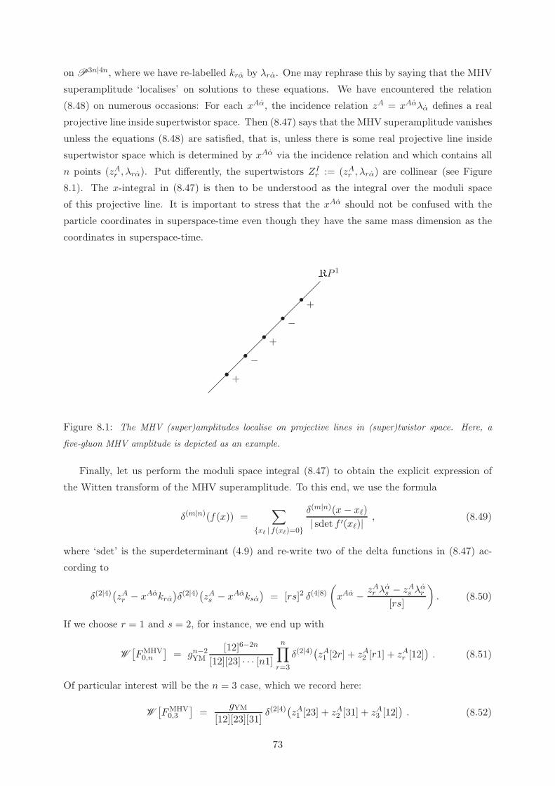
on P3n|4n, where we have re-labelled krα by λrα. One may rephrase this by saying that the MHV
superamplitude ‘localises’ on solutions to these equations. We have encountered the relation
(8.48) on numerous occasions: For each xAα, the incidence relation zA = xAαλα defines a real
projective line inside supertwistor space. Then (8.47) says that the MHV superamplitude vanishes
unless the equations (8.48) are satisfied, that is, unless there is some real projective line inside
supertwistor space which is determined by xAα via the incidence relation and which contains all
n points (zAr , λrα). Put differently, the supertwistors ZIr := (zAr , λrα) are collinear (see Figure
8.1). The x-integral in (8.47) is then to be understood as the integral over the moduli space
of this projective line. It is important to stress that the xAα should not be confused with the
particle coordinates in superspace-time even though they have the same mass dimension as the
coordinates in superspace-time.
+
−+
−+
RP 1
Figure 8.1: The MHV (super)amplitudes localise on projective lines in (super)twistor space. Here, a
five-gluon MHV amplitude is depicted as an example.
Finally, let us perform the moduli space integral (8.47) to obtain the explicit expression of
the Witten transform of the MHV superamplitude. To this end, we use the formula
δ(m|n)(f(x)) =∑
xℓ | f(xℓ)=0
δ(m|n)(x− xℓ)| sdet f ′(xℓ)|
, (8.49)
where ‘sdet’ is the superdeterminant (4.9) and re-write two of the delta functions in (8.47) ac-
cording to
δ(2|4)(zAr − xAαkrα
)δ(2|4)
(zAs − xAαksα
)= [rs]2 δ(4|8)
(
xAα − zAr λαs − zAs λαr[rs]
)
. (8.50)
If we choose r = 1 and s = 2, for instance, we end up with
W[FMHV0,n
]= gn−2
YM
[12]6−2n
[12][23] · · · [n1]n∏
r=3
δ(2|4)(zA1 [2r] + zA2 [r1] + zAr [12]
). (8.51)
Of particular interest will be the n = 3 case, which we record here:
W[FMHV0,3
]=
gYM
[12][23][31]δ(2|4)
(zA1 [23] + zA2 [31] + zA3 [12]
). (8.52)
73

Summarising, we see that MHV superamplitudes localise on projective lines in supertwistor
space. These are special instances of algebraic curves. In Section 9.5., we shall see that general
superamplitudes also localise on algebraic curves in supertwistor space. These localisation prop-
erties of scattering amplitudes are among the key results of [53]. This concludes our discussion
about MHV amplitudes.
Remark 8.2. Here, we have worked in a split signature space-time. However, one may
complexify and show that in a complex setting, the MHV (super)amplitudes also localise
on degree-one algebraic curves in (super)twistor space [53]. Put differently, the MHV (su-
per)amplitudes are supported on complex projective lines CP 1 in complex (super)twistor
space.
9. MHV formalism
In the preceeding sections, we have extensively discussed (colour-stripped) tree-level maximally-
helicity-violating amplitudes in both pure Yang–Mills theory and N = 4 supersymmetric Yang–
Mills theory. In the remainder of these lecture notes we would like to extend this discussion
beyond the MHV case and construct general tree-level scattering amplitudes.
One of the striking developments that came out of Witten’s twistor string theory is the MHV
formalism developed by Cachazo, Svrcek & Witten [114]. Recall that in the usual Feynman
diagram expansion, the interaction vertices are obtained from the (local) Lagrangian description
of the theory. In particular, interactions are supported on points in space-time. In the first part
of these lecture notes we have seen that points in space-time correspond to projective lines in
twistor space via the incidence relation (1.16). Furthermore, as explained in Section 8.4., MHV
amplitudes localise on projective lines in twistor space. So one can think of these amplitudes as
representing, in some sense, a generalisation of local interaction vertices. To take this analogy
further, one can try to build more complicated amplitudes from MHV amplitudes by gluing
together the latter in an appropriate way. As we shall see momentarily, the gluing is done with
the help of simple scalar propagators. In order for this to work, however, one has to continue
the MHV amplitudes off-shell. The resulting diagrammatic expansion of scattering amplitudes is
referred to as the MHV diagram expansion.
We begin by studying the MHV formalism in the pure Yang–Mills setting and then generalise
it to the N = 4 case. Before deriving this formalism from twistor space, however, we first set up
the basics and discuss some examples.
9.1. Cachazo–Svrcek–Witten rules
As indicated, we must continue the MHV amplitudes off-shell in order to use them as vertices
for general amplitudes. To this end, consider a generic momentum co-vector p with p2 6= 0. On
general grounds, it can always be decomposed into the sum of two null-momenta. We shall adopt
74
the following decomposition [115,116]:
p = q + tℓ , (9.1)
where q2 = 0, and ℓ is fixed but arbitrary with ℓ2 = 0. Here, t is some complex number which is
determined as a function of p according to
t =p2
2(p · ℓ) . (9.2)
Since q and ℓ are null, we may use co-spinors to represent them as qαβ = kαkβ and ℓαβ = ξαξβ.
It then follows that
kα =pαβξ
β
[kξ]and kα =
ξβpβα
〈ξk〉(9.3)
or in our above short-hand notation,
k =p|ξ][kξ]
and k =〈ξ|p〈ξk〉
(9.4)
These equations define our off-shell continuation (note that p2 6= 0 in the above formulæ): The
co-spinors k corresponding to the legs in the MHV amplitudes that are going to be taken off-
shell are represented by (9.4). Note that the denominators in (9.4) turn out to be irrelevant for
our applications since the expressions we are dealing with are homogeneous in the k that are
continued off-shell (see also below). Thus, we may discard the denominators and simply write
k = p|ξ] and k = 〈ξ|p . (9.5)
This is our off-shell formulation of MHV amplitudes. When continued off-shell, we shall often
refer to MHV amplitudes as MHV vertices. We complete the definition of the MHV or Cachazo–
Svrcek–Witten rules, by taking 1/p2 for the propagator connecting the MHV vertices.
Cachazo–Svrcek–Witten rules. The rules for computing colour-stripped tree-level scattering
amplitudes by gluing together MHV amplitudes are as follows:
(i) Use the MHV amplitudes as vertices.
(ii) For each leg of a vertex that joins with a propagator carrying momentum p, define its
corresponding co-spinor by k = 〈ξ|p, where ξ is some fixed spinor.
(iii) Glue the vertices together using scalar propagators 1/p2, where p is the momentum flowing
between the vertices. The two ends of any propagator must have opposite helicity labels, that
is, plus at one end and minus at the other.
The reader may wonder whether the amplitudes constructed this way actually depend on the
choice reference spinor ξ. In fact, it can be shown that this is not the case [114] and the resulting
overall amplitudes are indeed (Lorentz) covariant. This will also become transparent in Section
9.3., where we deduce the above rules from the twistor action (6.6a): ξ will arise as an ingredient
of a certain gauge condition. BRST invariance in turn guarantees that the overall amplitudes are
independent of ξ.
Note that a direct proof of these rules was given by Risager in [117].
75

MHV
MHV
MHV
+ +
+
+
−
−
−−
−
+−
+
Figure 9.1: A tree-level MHV diagram describing eight-gluon scattering with four gluons of positive helicity
and four gluons of negative helicity. Amplitudes with an equal number of positive and negative helicity
gluons are referred to as split helicity amplitudes. The amplitude displayed here is an N2MHV amplitude.
9.2. Examples
The Cachazo–Svrcek–Witten rules for joining together the MHV amplitudes are probably best
illustrated with an example.
A tree-level diagram with nV MHV vertices has 2nV positive-helicity legs, nV − 1 of which
are connected by propagators. According to rule (iii), each propagator must subsume precisely
one positive-helicity leg and therefore, we are left with 2nV − (nV − 1) = nV +1 external positive
helicities. Put differently, if we wish to compute a scattering amplitude with q positive helicity
gluons, we will need nV = q− 1 MHV vertices. Clearly, the MHV case is q = 2 and thus nV = 1.
In additon, this construction makes the vanishing of the amplitudes (8.1a) and (8.1b) (both for
the upper sign choice) manifest: In the former case, nV = −1 while in the latter case nV = 0.
The first non-trivial examples are obtained for q = 3 which are the NMHV amplitudes. We
shall denote them by ANMHV0,n (r+, s+, t+) or simply by ANMHV
0,n if there is no confusion. Thus, we
have schematically
ANMHV0,n =
∑
ΓL,ΓR|nL+nR=n+2AMHV
0,nL(ΓL)
1
p2L,RAMHV
0,nR(ΓR)
=∑
ΓL,ΓR|nL+nR=n+2
pnL−1
p1
pnL
pn
ΓL ΓR1/p2L,R
(9.6)
76

where the sum is taken over all possible MHV vertices ΓL,R contributing to the amplitude such
that nL + nR = n+ 2 and nL,R ≥ 3. One may check that there are a total of n(n− 3)/2 distinct
diagrams contributing to this sum (see e.g. [118,119]).
The simplest example of an NMHV amplitude is the four-gluon amplitude ANMHV0,4 (2+, 3+, 4+)
= A0,4(1−, 2+, 3+, 4+). This amplitude is of the type (8.1b) for the lower sign choice and hence,
it should vanish. Let us demonstrate this by using the above rules. The relevant diagrams
contributing to this amplitude are depicted in Figure 9.2. For each diagram we should write
down the MHV amplitudes corresponding to each vertex and join them together with the relevant
propagator, remembering to use the above off-shell continuation to deal with the co-spinors
associated with the internal lines. Let us start with diagram (a). We have k = 〈ξ|p and therefore
(a) =[2k]4
[k1][12][2k]
1
p2[34]4
[4k][k3][34]=
[2k]3
[k1][12]
1
p2[34]3
[4k][k3], (9.7)
where
p = −p1 − p2 = p3 + p4 (9.8)
due to momentum conservation. Note that p2r = 0 and therefore, prαβ = krαkrβ for r = 1, . . . , 4.
Next we define cr := 〈ξkr〉. Hence,
k = −c1k1 − c2k2 = c3k3 + c4k4 , (9.9)
which follows from (9.8) upon contracting with ξ. This last equation can in turn be used to
compute the quantities [kr] which can then be substituted into (9.7). Noting that p2 = −2p1 · p2,we eventually arrive at
(a) = − c314c2c3c4
[34]
〈12〉 . (9.10)
p1
p2 p3
p4−
+ +
+
+
−1/p2
MHV
MHV
(b)
MHV MHV
p2
p1
p3
p4
+
−
+
++ −1/p2
(a)
Figure 9.2: The two diagrams contributing to the −+++ amplitude. All external momenta are taken to
be incoming.
Going through the same procedure for the second diagram in Figure 9.2 gives
(b) =c31
4c2c3c4
〈23〉[14]
(9.11)
77
and therefore,
(a) + (b) = − c314c2c3c4
([34]
〈12〉 −[23]
〈14〉
)
. (9.12)
Momentum conservation is∑
r pr =∑
r krkr = 0 and upon contracting this equation with k3,
one realises that [34]〈14〉 = [23]〈12〉. Altogether, (a) + (b) = 0 as expected. For all the NMHV
amplitudes, see e.g. [115,120,118,119].
Exercise 9.1. Derive the five-gluon NMHV amplitude
ANMHV0,5 (2+, 4+, 5+) = A0,5(1
−, 2+, 3−, 4+, 5+)
using the above rules. You should find 5(5 − 3)/2 = 5 diagrams that contribute to the
amplitude. Notice that this amplitude is actually an MHV amplitude and according to
(8.1d), you should find 〈13〉4/(〈12〉〈23〉 · · · 〈51〉).
The MHV diagram expansion has been implemented both for amplitudes with more external
gluons and amplitudes with more positive helicities. In both cases the complexity grows, but
the number of diagrams one has to consider follows a power growth for large n (e.g. n2 for the
NMHV diagrams [114]) which is a marked improvement on the factorial growth of the number of
Feynman diagrams needed to compute the same process; see Table 7.1.
9.3. MHV diagrams from twistor space
Let us now examine the Cachazo–Svrcek–Witten rules in the context of the twistor action (6.6a).
The canonical way of deriving a perturbative or diagrammatic expansion of some theory that is
described by some action functional is to fix the gauge symmetries first and then to derive the
corresponding propagators and vertices. As we shall see momentarily, there exists a gauge for the
twistor space action (6.6a) that leads directly to the Cachazo–Svrcek–Witten rules, that is, to the
perturbative expansion of Yang–Mills theory in terms of MHV diagrams. For concreteness, we
again assume that Euclidean reality conditions have been imposed. The subsequent discussion
follows [66,67] closely (see also [121,122]). For a treatment of perturbative Chern–Simons theory,
see e.g. [123,124].
As we wish to describe pure Yang–Mills theory here, we assume that only A and G are present
in the superfield expansion (5.40). Thus,
A0,1 = A+ 14!ηiηjηkηlε
ijklG = A+ (η)4G , (9.13)
where we have used the notation of (6.14). As before, we shall use the circles to denote the
component fields. Upon substituting the above expansion into the holomorphic Chern–Simons
part of the action (6.6a), we arrive at
S =
∫
Ω0 ∧ trG ∧ (∂A+A ∧A)
(9.14)
78

once the fermionic coordinates are integrated over. Notice that we have re-scaled the measure Ω0
in order to get rid of certain numerical pre-factors which are not essential for the discussion that
follows.
Furthermore, using
A = e0A0 + eαAα and G = e0G0 + eαGα , (9.15)
we may perform an analysis similar to (6.12) to find the contribution coming from (6.6b):
tr log∇0,1|Lx = tr log(∂ +A+ (η)4G
)|Lx
= trlog(∂ +A
)|Lx + log
[1 + (η)4(∂ +A)−1G
]|Lx
= tr
log(∂ +A
)|Lx +
∞∑
r=1
(−1)rr
∫
Lx
r∏
s=1
K(λs) (ηs)4GA(λs−1, λs)G0(λs)
. (9.16)
Here, GA(λ, λ′) is the Green function of the (∂ +A)|Lx -operator on the projective line Lx,
(∂ +A)−1ω(λ)|Lx =
∫
Lx
K(λ′)GA(λ, λ′)ω0(λ′) , for ω = e0ω0 + eαωα , (9.17)
and K(λ) is the Kahler form on Lx which was introduced in Remark 5.5. Now we may employ
Nair’s lemma (6.14) and integrate over d8η in (9.16) to obtain the following form of the action
(6.6b):
Sε = −1
2ε
∫
d4x
∫
Lx
K(λ1)K(λ2)[12]4 tr GA(λ2, λ1)G0(λ1)GA(λ1, λ2)G0(λ2) . (9.18)
Altogether, the twistor space action (6.6a) reduces to the Mason twistor action [66]:
Stot =
∫
Ω0 ∧ trG ∧ (∂A+A ∧A)
− 1
2ε
∫
d4x
∫
Lx
K(λ1)K(λ2)[12]4 tr GA(λ2, λ1)G0(λ1)GA(λ1, λ2)G0(λ2)
(9.19)
of pure Yang–Mills theory.
Finally, we need to find an explicit expression for the Green function GA(λ, λ′). Obviously,
for A0 = 0, GA(λ, λ′) coincides with the Green function G(λ, λ′) for the ∂|Lx-operator as given
in (6.10). For A0 6= 0, we have the expansion
(∂ +A)−1|Lx = ∂−1|Lx − ∂−1A ∂−1|Lx + ∂−1A ∂−1A ∂−1|Lx + · · · . (9.20)
With the help of (6.10) and (9.17), this can be re-written according to
GA(λ, λ′) = G(λ, λ′) +
∞∑
r=1
(−1)r∫
Lx
(r∏
s=1
K(λs)G(λs−1, λs)A0(λs)
)
G(λr, λ′) , (9.21)
with λ0 ≡ λ. This expression may now be substituted into the Mason action (9.19) to obtain
Stot =
∫
Ω0 ∧ trG ∧ (∂A+A ∧A)
− 1
2ε
∫
d4x∞∑
r=2
(−1)r∫
Lx
(r∏
s=1
K(λs)G(λs−1, λs)
)
×r∑
t=2
[1t]4 tr G0(λ1)A0(λ2) · · · A0(λt−1)G0(λt)A0(λt+1) · · · A0(λr) .
(9.22)
79

Notice that the infinite sum strongly resembles a sum of MHV vertices (recall that G carries
helicity +1 while A carries helicity −1). Also notice that (9.22) is invariant under the following
gauge transformations:
δA = ∂α+ [A,α] and δG = ∂β + [A, β] + [G,α] , (9.23)
where α and β are smooth functions of homogeneities 0 and −4, respectively. Notice that these
transformations are an immediate consequence of (5.21).
Next we would like to restore the dependence on the Yang–Mills coupling constant gYM in
Stot that is compatible with the perturbation theory we have discussed so far. Remember from
our discussion in Section 6.1. that in this perturbative context, the parameter ε is identified with
g2YM. Rescaling A as A 7→ gYMA and G as G 7→ g−1YMG, respectively, we find
Stot =
∫
Ω0 ∧ trG ∧ (∂A+ gYMA ∧A)
− 1
2
∫
d4x
∞∑
r=2
(−1)rgr−2YM
∫
Lx
(r∏
s=1
K(λs)G(λs−1, λs)
)
×r∑
t=2
[1t]4 tr G0(λ1)A0(λ2) · · · A0(λt−1)G0(λt)A0(λt+1) · · · A0(λr) .
(9.24)
Let us now decompose this expression as
Stot = Skin + Sint , (9.25a)
where
Skin :=
∫
Ω0 ∧ trG ∧ ∂A
Sint := gYM
∫
Ω0 ∧ tr G ∧A ∧A
− 1
2
∫
d4x∞∑
r=2
(−1)rgr−2YM
∫
Lx
(r∏
s=1
K(λs)G(λs−1, λs)
)
×r∑
t=2
[1t]4 tr G0(λ1)A0(λ2) · · · A0(λt−1)G0(λt)A0(λt+1) · · · A0(λr) .
(9.25b)
Note that the first term in the infinite sum of Sint contains a term that is quadratic in G and
that involves no A fields. We are always free to treat this term either as a vertex or as part of
the kinetic energy, but as our re-writing already suggests, we shall do the former.
After some algebraic manipulations, the interaction part Sint can be further re-written:
Sint = gYM
∫
Ω0 ∧ tr G ∧A ∧A
−∫
d4x
∞∑
r=2
(−1)rr!
gr−2YM
∑
σ∈Sr/Zr
∫
Lx
(r∏
s=1
K(λσ(s))G(λσ(s−1), λσ(s))
)
×∑
s<t
[σ(s)σ(t)]4 trA0(λσ(1)) · · · A0(λσ(s−1))G0(λσ(s))A0(λσ(s+1)) · · ·
· · · A0(λσ(t−1))G0(λσ(t))A0(λσ(t+1)) · · · A0(λσ(r)).
(9.26)
80

Here, Sr is the permutation group of degree r and Zr is the group of cyclic permutations of order
r.
In order to proceed further, we need to fix the gauge symmetries; see (9.23). In Sections 5.2.
and 6.2. we partially fixed the gauge symmetries by imposing the space-time gauge (5.41). This
partial gauge-fixing turned out to be suitable for deriving the usual space-time action from the
twistor action. However, we may certainly impose other gauges and the one that will eventually
yield the Cachazo–Svrcek–Witten rules is the following:
ξα1 VαyA = 0 = ξα2 VαyG (9.27)
for some fixed but arbitrary spinors ξ1 and ξ2. This is an axial gauge, so the corresponding ghost
terms will decouple. Notice that this gauge choice differs somewhat from the one of [66,67]27 since
here we are using two a priori different spinors ξ1 and ξ2. Any solution to these gauge constraints
is of the form
Aα = ξ1αA and Gα = ξ2αG (9.28)
for some smooth functions A and G of homogeneities 1 and −3 (remember that Aα and Gα are
of these homogeneities).
Having chosen gauge fixing conditions, we are now in a position to derive the propagator or
the Green function of the ∂-operator on twistor space P 3. Upon using (9.15), Skin is explicitly
given by
Skin =
∫Ω0 ∧ Ω0
[λλ]4trGα(V0Aα − VαA0) +G0VαA
α. (9.29)
On solutions (9.28) to the gauge constraints (9.27), this becomes
Skin,gf =
∫
d4xK(λ) tr
(
G0 , G)(
0 ξα1 Vα
−ξα2 Vα 〈ξ2ξ1〉V0
)(
A0
A
)
=
∫d4p
(2π)4K(λ) tr
(
G0 , G)
(p)
(
0 i〈ξ1|p|λ]−i〈ξ2|p|λ] 〈ξ2ξ1〉V0
)(
A0
A
)
(−p)
,
(9.30)
where in the first step we have used (5.52) to re-write the measure in (9.29) while in the second
step we have performed a Fourier transform on the x-coordinates.
Next it is useful to introduce certain differential (0, 1)-form-valued weighted delta functions
of spinor products [114,67],
δ(m)([λ1λ2]) :=
([λ1ξ]
[λ2ξ]
)m+1
∂(λ2)1
[λ1λ2](9.31)
where ξ is some constant spinor. Using (6.9a), this is explicitly
δ(m)([λ1λ2]) =[dλ2λ2]
[λ2λ2]2︸ ︷︷ ︸
= e0(λ2)
(−2π)[λ2λ2]2([ξλ1]
[ξλ2]
)m+1 [ξλ1]
[ξλ2]δ(2)([λ1λ2], [λ1λ2])
︸ ︷︷ ︸
=: δ0(m)
([λ1λ2])
= e0(λ2) δ0(m)([λ1λ2]) .
(9.32)
27See also [125] for a similar treatment.
81

This expression is independent of ξ since on support of the delta function we have λ1 ∝ λ2. Notethat under a re-scaling λ1,2 7→ t1,2λ1,2 for t1,2 ∈ C \ 0, we have
δ(m)([λ1λ2]) 7→ tm1 t−m−22 δ(m)([λ1λ2]) and δ0(m)([λ1λ2]) 7→ tm1 t
−m2 δ0(m)([λ1λ2]) . (9.33)
Using (9.31), Skin,gf given by (9.30) becomes
Skin,gf =
∫d4p
(2π)4K(λ1)K(λ2)
× tr
(
G0 , G)
(p, λ1)
(
0 K1(λ1, λ2)
K2(λ1, λ2) K3(λ1, λ2)
)(
A0
A
)
(−p, λ2)
,
(9.34a)
where
K(λ1, λ2) :=
(
0 K1(λ1, λ2)
K2(λ1, λ2) K3(λ1, λ2)
)
:= − 1
2π
(
0 iδ0(2)([λ1λ2])〈ξ1|p|λ2]−iδ0(3)([λ1λ2])〈ξ2|p|λ2] δ0(3)([λ1λ2])〈ξ2ξ1〉V0(λ2)
) (9.34b)
The Green function or propagator G(λ1, λ2),
G(λ1, λ2) :=
(
G1(λ1, λ2) G2(λ1, λ2)G3(λ1, λ2) 0
)
=
(
〈A0(p, λ1)B0(−p, λ2)〉 〈A0(p, λ1)B(−p, λ2)〉〈A(p, λ1)B0(−p, λ2)〉 0
) (9.35)
is determined by ∫
K(λ3)K(λ1, λ3)G(λ3, λ2) = I(λ1, λ2) , (9.36)
where I(λ1, λ2) is the identity
I(λ1, λ2) := − 1
2π
(
δ0(2)([λ1λ2]) 0
0 δ0(−3)([λ2λ1])
)
. (9.37)
A short calculation shows that
G1(λ1, λ2) =1
2π
〈ξ2ξ1〉〈ξ2|p|λ1]
(
V0(λ1)1
〈ξ1|p|λ1]
)
δ0(2)([λ1λ2]) ,
G2(λ1, λ2) =1
2πi
δ0(−3)([λ2λ1])
〈ξ2|p|λ2],
G3(λ1, λ2) = − 1
2πi
δ0(2)([λ1λ2])
〈ξ1|p|λ1].
(9.38)
The propagator G1 may be simplified further to give
G1(λ1, λ2) =1
2π
〈ξ2ξ1〉〈ξ2|p|λ1]
〈ξ1|p|ξ][λ1ξ]
δ0(−2)(〈ξ1|p|λ1]) δ0(2)([λ1λ2])
= − 1
2π
4
p2δ0(−2)(〈ξ1|p|λ1]) δ0(2)(〈ξ1|p|λ2]) ,
(9.39)
82

where in the first step we have inserted the definition (9.32) while in the second step we have
used the fact that λ1 ∝ 〈ξ1|p on support of the first delta function together with the identity
pααpβα = 1
4p2δβα.
Altogether, we arrive at
G(λ1, λ2) = − 1
2π
4p2δ0(−2)(〈ξ1|p|λ1]) δ0(2)(〈ξ1|p|λ2]) i
〈ξ2|p|λ2]δ0(−3)([λ2λ1])
− i〈ξ1|p|λ1]
δ0(2)([λ1λ2]) 0
. (9.40)
A particularly simple form of the propagator is achieved for the choice ξ1 → ξ and ξ2 → ξ.
We shall refer to this gauge as Cachazo–Svrcek–Witten gauge, and the reason for its name will
become apparent momentarily. Upon multiplying (9.35), (9.40) by the appropriate differential
forms e0 and eα and by ξα, our final result for the propagator is [67]
〈A(p, λ1) ∧ B(−p, λ2)〉 = − 1
2π
[
4
p2δ(−2)(〈ξ|p|λ1]) ∧ δ(2)(〈ξ|p|λ2])
+δ(−3)([λ2λ1]) ∧ 〈ξe(λ2)〉
i〈ξ|p|λ2]− 〈ξe(λ1)〉 ∧ δ(2)([λ1λ2])
i〈ξ|p|λ1]
]
.
(9.41)
Having constructed the propagator, we shall now take a closer look at the vertices appearing
in (9.26). One pleasing feature of the Cachazo–Svrcek–Witten gauge is that the interaction vertex
G∧A∧A does not contribute. Therefore, the only remaining interactions come from the infinite
sum in (9.26). We shall now show that these are the MHV vertices, i.e. the on-shell version of
(9.26) does indeed give rise to the MHV amplitudes.
Recall from Theorem 2.2. that solutions to the zero-rest-mass field equations of helicity h ∈ 12Z
are given by elements of the Cech cohomology group H1(P 3,O(−2h − 2)). By Remark 5.6. we
know that H1(P 3,O(−2h − 2)) ∼= H0,1∂
(P 3,O(−2h − 2)). Therefore, solutions to free field equa-
tions may equivalently be described in terms of differential (0, 1)-forms ω−2h−2 of homogeneity
−2h− 2. In particular, the plane wave solutions of momentum p = kk which were constructed in
Section 7.3. arise from
ω−2h−2(z, λ) = δ(2h)[kλ]) exp
(
i〈zk〉 [kξ][λξ]
)
(9.42)
by suitably integrating over∫
Lx[dλλ]. For more details, see Exercise 9.2. As before, the parameter
ξ plays no role since on support of the delta function λ ∝ k.
Exercise 9.2. Show that the wavefunction (7.16) arises from∫
Lx[dλλ]∧ω−2. Show further
that the h = ±12 wavefunctions (7.17) are given by
∫
Lx[dλλ]∧λαω−3 and
∫
Lx[dλλ]∧ ∂αω−1
where ∂α := ∂/∂zα.
Notice that the twistor space wavefunctions (9.42) obey the Cachazo–Svrcek–Witten gauge
condition, since there are no components along eα. Therefore, we may take
A(x, λσ(s)) = tσ(s)δ(−2)[kσ(s)λσ(s)]) exp
(
i〈zσ(s)kσ(s)〉[kσ(s)ξ]
[λσ(s)ξ]
)
,
G(x, λσ(s)) = tσ(s)δ(2)[kσ(s)λσ(s)]) exp
(
i〈zσ(s)kσ(s)〉[kσ(s)ξ]
[λσ(s)ξ]
)
,
(9.43)
83

where tσ(s) is an arbitrary element of the Lie algebra of the gauge group. Inserting these wave-
functions and the Green function (6.10) into (9.26), one may trivially perform the λ-integrals by
replacing λσ(s) by kσ(s). The final x-integral then gives an overall delta function of momentum
conservation. The result of these rather straightforward manipulations is
Sint,gf =
∞∑
r=0
(i gYM)r−2(2π)4δ(4)
(r∑
s=1
ksks
)
× 1
r!
∑
σ∈Sr/Zr
∑
s<t[kσ(s)kσ(t)]4
[kσ(r)kσ(1)][kσ(1)kσ(2)] · · · [kσ(r−1)kσ(r)]trtσ(1) · · · tσ(r) .
(9.44)
This, however, is a sum over all the MHV amplitudes (8.1c) including the appropriate colour-trace
factors (see also (7.10)).
Let us now summarise these results. We have shown28 that the twistor space action (6.6a)
indeed gives the MHV diagram expansion once the Cachazo–Svrcek–Witten gauge (9.27) with
ξ1,2 → ξ has been imposed: Firstly, for this choice of gauge, the interaction vertices come solely
from the second part of (9.26) and as we have just seen, these vertices coincide with the MHV
amplitudes when put on-shell. This is the first of the Cachazo–Svrcek–Witten rules. Secondly,
the delta functions in the propagator (9.41) lead to the prescription for the insertion of k = 〈ξ|pas the co-spinor corresponding to the off-shell momentum p. This is the second Cachazo–Svrcek–
Witten rule. Lastly, the third rule also follows from (9.41) due to the explicit appearance of
1/p2. Thus, we have obtained the Cachazo–Svrcek–Witten rules directly from twistor space. As
already indicated, since the spinor ξ arises here as part of the gauge condition, BRST invariance
ensures that the overall amplitudes will not depend on it.
Finally, we would like to emphasise that the above procedure makes manifest the equival-
ence between the traditional Feynman diagram expansion and the MHV diagram expansion for
Yang–Mills theory: The space-time Yang–Mills action including the resulting Feynman diagram
expansion on the one side and the action or generating functional yielding the MHV diagram
expansion on the other side are merely consequences of different gauge choices for the twistor
space action. This is possible since the gauge symmetry of the twistor space action, being defined
on a real six-dimensional manifold, is much larger than that of the Yang–Mills action on four-
dimensional space-time. Note that the described equivalence can only be valid at tree-level in
perturbation theory, since in pure Yang–Mills theory at loop-level there are diagrams that can-
not be constructed from MHV vertices and propagators alone. See e.g. [126] for a full discussion.
Therefore, even though the space-time gauge (5.41) yields the fully fledged Yang–Mills action, the
above derivation of the MHV diagrams appears to work only at tree-level (and so do the Cachazo–
Svrcek–Witten rules stated in the preceding section).29 Presumably, the issue with loops is due
to the following two problems. The first problem, as argued in [67], lies in the change of the path
integral measure: When going from the space-time gauge to the Cachazo–Svrcek–Witten gauge
one must perform a complex gauge transformation while the path integral is only invariant under
28See also [125] for a more detailed exposition of this material.29See [127–131] for an extension of the Cachazo–Svrcek–Witten rules to one-loop level.
84
real gauge transformations. The second problem has to do with certain regularisation issues as
discussed in [132]. As we are only concerned with tree-level scattering amplitudes in these lecture
notes, we shall not worry about these issues any further.
Remark 9.1. Let us point out that there is an alternative (but equivalent [132]) approach
that maps the ordinary Yang–Mills action to a functional where the vertices are explicitly
the MHV vertices. This approach has been developed by Mansfield in [133] (see also [134–
136,126]). For a recent review, see [137]. This approach works directly in four-dimensional
space-time and involves formulating Yang–Mills theory in light-cone gauge and performing
a non-local field transformation. In similarity with the twistor space approach above, the
spinor ξ arises in fixing the light-cone gauge. Finally, let us mention in passing that the
above procedure has also been extended to gravity [122] (see also [138–142] ) using the gravity
twistor space action of [64] (see also [143]).
9.4. Superamplitudes in the MHV formalism
So far, we have discussed the MHV formalism in pure Yang–Mills theory only. Let us now briefly
explain how the above discussion extends to the N = 4 supersymmetric theory.
In Section 8.2., we have seen that all the different scattering amplitudes occuring in N = 4
supersymmetric Yang–Mills theory are encoded in terms of certain superamplitudes which we
also called generating functions. In particular, all the different (colour-stripped) MHV amplitudes
follow from Nair’s formula (8.17) via (8.21). The question then arises of: How do we generalise
(8.17) to NkMHV scattering amplitudes, that is, how can we encode all the NkMHV amplitudes
in terms of NkMHV superamplitudes with a relationship similar to (8.21)?
To answer this question, let us first recall that the total helicity of an n-particle NkMHV scat-
tering amplitude is −n+2k+4 while an n-particle superamplitude has always a total helicity of
−n. Notice that k = 0, . . . , n− 4 since AN0MHVn ≡ AMHV
n and ANn−4MHVn = AMHV
n . Furthermore,
as we have explained in Section 8.2., the differential operators (8.14) will pick from a superamp-
litude the appropriate particles one wishes to scatter (i.e. the external states). This therefore
suggests that an n-particle NkMHV superamplitude FNkMHVn is a homogeneous polynomial of
degree 2(2k+4) = 4k+8 in the fermionic coordinates ψir: Each ψir carries a helicity of −1/2 and
therefore, a differential operator D(4k+8) of order 4k+8 that is made of the operators (8.14) will
have a total helicity of 2k+4. Consequently, D(4k+8)FNkMHVn will carry a helicity of −n+2k+4,
as desired.
Besides this, the superamplitudes are supersymmetric by construction and so they are anni-
hilated by the Poincare supercharges Qiα and Qiα and by the generator of space-time translations
Pαβ . Since Qiα and Pαβ are represented by multiplication operators (8.2), (8.22) when acting
on superamplitudes, the latter must be proportional to the overall delta function (8.16) of (su-
85
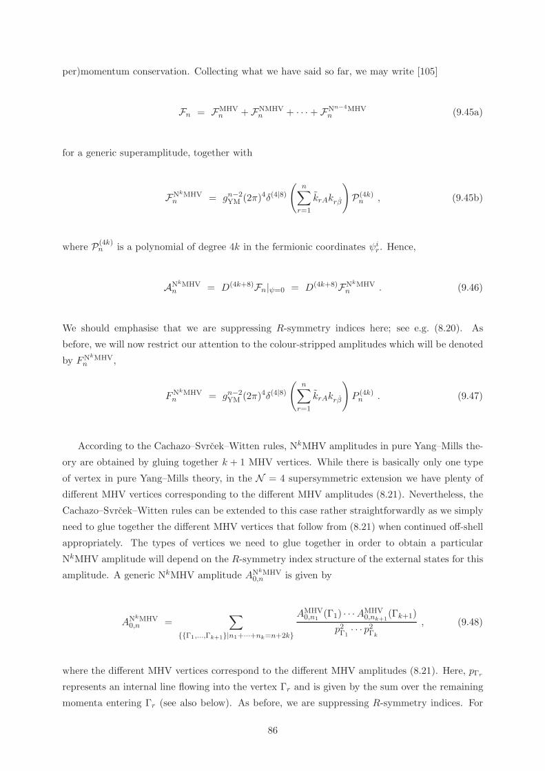
per)momentum conservation. Collecting what we have said so far, we may write [105]
Fn = FMHVn + FNMHV
n + · · · + FNn−4MHVn (9.45a)
for a generic superamplitude, together with
FNkMHVn = gn−2
YM (2π)4δ(4|8)(
n∑
r=1
krAkrβ
)
P(4k)n , (9.45b)
where P(4k)n is a polynomial of degree 4k in the fermionic coordinates ψir. Hence,
ANkMHVn = D(4k+8)Fn|ψ=0 = D(4k+8)FNkMHV
n . (9.46)
We should emphasise that we are suppressing R-symmetry indices here; see e.g. (8.20). As
before, we will now restrict our attention to the colour-stripped amplitudes which will be denoted
by FNkMHVn ,
FNkMHVn = gn−2
YM (2π)4δ(4|8)(
n∑
r=1
krAkrβ
)
P (4k)n . (9.47)
According to the Cachazo–Svrcek–Witten rules, NkMHV amplitudes in pure Yang–Mills the-
ory are obtained by gluing together k + 1 MHV vertices. While there is basically only one type
of vertex in pure Yang–Mills theory, in the N = 4 supersymmetric extension we have plenty of
different MHV vertices corresponding to the different MHV amplitudes (8.21). Nevertheless, the
Cachazo–Svrcek–Witten rules can be extended to this case rather straightforwardly as we simply
need to glue together the different MHV vertices that follow from (8.21) when continued off-shell
appropriately. The types of vertices we need to glue together in order to obtain a particular
NkMHV amplitude will depend on the R-symmetry index structure of the external states for this
amplitude. A generic NkMHV amplitude ANkMHV0,n is given by
ANkMHV0,n =
∑
Γ1,...,Γk+1|n1+···+nk=n+2k
AMHV0,n1
(Γ1) · · ·AMHV0,nk+1
(Γk+1)
p2Γ1· · · p2Γk
, (9.48)
where the different MHV vertices correspond to the different MHV amplitudes (8.21). Here, pΓr
represents an internal line flowing into the vertex Γr and is given by the sum over the remaining
momenta entering Γr (see also below). As before, we are suppressing R-symmetry indices. For
86

instance, we have
ANMHV0,n =
∑
Γ1,Γ2|n1+n2=n+2AMHV
0,n1(Γ1)
1
p2Γ1
AMHV0,n2
(Γ2)
=∑
Γ1 Γ2
1/p2Γ1 (9.49a)
AN2MHV0,n =
∑
Γ1,Γ2,Γ3|n1+n2+n3=n+4
AMHV0,n1
(Γ1)AMHV0,n2
(Γ2)AMHV0,n3
(Γ3)
p2Γ1p2Γ2
p2Γ3
=∑
Γ1 Γ3 Γ2
1/p2Γ11/p2Γ2 (9.49b)
for the NMHV and N2MHV amplitudes, while for the N3MHV amplitudes we have two different
graph topologies:
AN3MHV0,n =
∑
Γ1,...,Γ4|n1+···+n4=n+6
AMHV0,n1
(Γ1) · · ·AMHV0,n4
(Γ4)
p2Γ1p2Γ2
p2Γ3
=∑
Γ1 Γ2 Γ4 Γ3
1/p2Γ11/p2Γ2
1/p2Γ3
+∑
Γ1 Γ4
Γ2
Γ31/p2Γ1
1/p2Γ2
1/p2Γ3
(9.49c)
Similarly, one may draw the diagrams contributing to the NkMHV amplitude for larger and larger
k but, of course, the complexity in the graph topology will grow. In this notation, Figure 9.2
becomes:
87
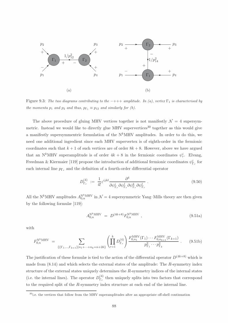
p1
p2 p3
p4−
+ +
+
+
−1/p214
Γ2
Γ1
(b)
Γ1 Γ2
p2
p1
p3
p4
+
−
+
++ −1/p212
(a)
Figure 9.3: The two diagrams contributing to the −+++ amplitude. In (a), vertex Γ1 is characterised by
the momenta p1 and p2 and thus, pΓ1≡ p12 and similarly for (b).
The above procedure of gluing MHV vertices together is not manifestly N = 4 supersym-
metric. Instead we would like to directly glue MHV supervertices30 together as this would give
a manifestly supersymmentric formulation of the NkMHV amplitudes. In order to do this, we
need one additional ingredient since each MHV supervertex is of eighth-order in the fermionic
coordinates such that k + 1 of such vertices are of order 8k + 8. However, above we have argued
that an NkMHV superamplitude is of order 4k + 8 in the fermionic coordinates ψir. Elvang,
Freedman & Kiermaier [119] propose the introduction of additional fermionic coordinates ψiΓrfor
each internal line pΓr and the definition of a fourth-order differential operator
D(4)Γr
:=1
4!εijkl
∂4
∂ψiΓr∂ψjΓr
∂ψkΓr∂ψlΓr
. (9.50)
All the NkMHV amplitudes ANkMHV0,n in N = 4 supersymmetric Yang–Mills theory are then given
by the following formulæ [119]:
ANkMHV0,n = D(4k+8)FNkMHV
0,n , (9.51a)
with
FNkMHV0,n =
∑
Γ1,...,Γk+1|n1+···+nk=n+2k
(k∏
r=1
D(4)Γr
)
FMHV0,n1
(Γ1) · · ·FMHV0,nk+1
(Γk+1)
p2Γ1· · · p2Γk
. (9.51b)
The justification of these formulæ is tied to the action of the differential operator D(4k+8) which is
made from (8.14) and which selects the external states of the amplitude: The R-symmetry index
structure of the external states uniquely determines the R-symmetry indices of the internal states
(i.e. the internal lines). The operator D(4)Γr
then uniquely splits into two factors that correspond
to the required split of the R-symmetry index structure at each end of the internal line.
30i.e. the vertices that follow from the MHV superamplitudes after an appropriate off-shell continuation
88

The expression (9.51b) can be simplified further. We shall just state the result here and refer
the interested reader to [119] for the explicit derivation. We have
FNkMHV0,n = gn−2
YM (2π)4δ(4|8)(
n∑
r=1
krAkrβ
)
P(4k)0,n , (9.52a)
with
P(4k)0,n =
∑
Γ1,...,Γk+1|n1+···+nk=n+2k
∏kr=1
1p2Γr
∑
s∈Γr〈ξ|pΓr |ks](ψs)4
cyc(Γ1) · · · cyc(Γk+1). (9.52b)
Here, we have used the notation (6.14) for ψis and ‘cyc’ denotes the usual denominator of the
spinor brackets appearing in the MHV amplitudes, e.g. cyc(1, . . . , n) := [12] · · · [n1]. In addition,
the external momenta are pr = krkr for r = 1, . . . , n. Note that the result for the tree-level
NMHV superamplitude was first obtained by Georgiou, Glover & Khoze in [120]. In [144], a
refined version of (9.52b) was given in which the number of diagrams one needs to sum over is
reduced substantially.
Next one should show that this expression is independent of the choice of the spinor ξ that
defines the off-shell continuation. This was done explicitly in [119]. Notice, however, that ana-
logously to our discussion presented in Section 9.3., ξ can also be shown to arise from a gauge
fixing condition of the twistor space action (6.6a). This time, of course, one should include the
full supermultiplet (5.40). Therefore, BRST invariance will guarantee the ξ-independence of the
overall scattering amplitudes.
Remark 9.2. Note that there is an alternative method [145] for constructing the polyno-
mials P(4k)n occurring in (9.45). Drummond & Henn [145] express the P(4k)
n in terms of
invariants of the so-called dual superconformal symmetry group [146–151,105,152–160] (see
also [161–165] and [166–168] for recent reviews). The dual superconformal symmetry is a
recently discovered hidden (dynamical) symmetry, planar scattering amplitudes in N = 4
supersymmetric Yang–Mills theory appear to exhibit.
9.5. Localisation properties
In this section, we would like to comment on the localisation properties of generic scattering
amplitudes in twistor space. In Section 8.4., we saw that MHV superamplitudes localise on
genus-0 degree-1 curves Σ in supertwistor space: Σ ∼= CP 1 in the complex setting or Σ ∼= RP 1
in the Kleinian setting. According to the MHV formalism, generic tree-level superamplitudes are
obtained by gluing the MHV superamplitudes together (after a suitable off-shell continuation).
This is depicted in Figure 9.4 for the case of NMHV amplitudes.
This therefore suggests that tree-level NkMHV superamplitudes localise on maximally discon-
nected rational curves Σ of genus zero, that is, each Σ is the union of k + 1 (projective) lines in
supertwistor space. Therefore, the total degree d of each Σ is
d = k + 1 . (9.53)
89

Figure 9.4: An NMHV amplitude represented in twistor space: Each line represents an MHV amplitude
(or vertex) while the dotted line represents the propagator of holomorphic Chern–Simons theory; see (9.41)
for the case of pure Yang–Mills theory.
This picture is the so-called maximally disconnected description of scattering amplitudes. As
was observed in [169–171], scattering amplitudes may also be described by completely connected
rational curves. In particular, tree-level NMHV superamplitudes may also be described by con-
nected genus-0 degree-2 rational curves as is depicted in Figure 9.5. This is referred to as the
connected description of scattering amplitudes. It was argued, however, by Gukov, Motl & Neitzke
in [172] that the two descriptions—that is, the disconnected and connected prescriptions—are in
fact equivalent.
Figure 9.5: An NMHV amplitude described by a connected degree-2 rational curve in supertwistor space.
In general, the conjecture put forward by Witten [53] is that ℓ-loop NkMHV superamplitudes
localise on rational curves in supertwistor space which are of genus g ≤ ℓ and degree
d = k + 1 + g . (9.54)
Following the earlier work of [173, 174, 106, 175], Korchemsky & Sokatchev [176] (see also [177,
110,178–181]) performed the Witten transform (8.43) of all tree-level scattering amplitudes expli-
citly. In fact, they transformed the Drummond & Henn expressions [145] of the quantities P(4k)n
90
appearing in (9.45) for the NkMHV superamplitudes to supertwistor space. They found that
the NkMHV superamplitudes are supported on 2k + 1 intersecting lines in supertwistor space in
contra-distinction to what we have said above (9.53). This puzzle was resolved very recently by
Bullimore, Mason & Skinner in [182] (see also [183]) by proving that the Drummond & Henn ex-
pressions for the tree-level amplitudes actually contain loop-level information: They showed that
the 2k+1 intersecting lines form a curve of genus g = k and therefore, d = k+1+ k = k+1+ g.
Their result generalises the fact [180,155] that the tree-level NMHV superamplitudes can be writ-
ten in terms of loop-level information31. Altogether, the result of Korchemsky & Sokatchev [176]
is therefore in support of Witten’s conjecture (9.54).
10. Britto–Cachazo–Feng–Witten recursion relations
Central to this final section will be the dicussion of a powerful method for constructing tree-level
amplitudes first introduced by Britto, Cachazo & Feng in [193] (stemming from observations
made in [194]) and later proven by Britto, Cachazo, Feng & Witten in [195]. We shall start with
pure Yang–Mills theory and closely follow the treatment of [195] before moving on to the N = 4
supersymmetric extension developed by [142,154,196].
10.1. Recursion relations in pure Yang–Mills theory
The basic philosophy of the method developed by Britto, Cachazo, Feng & Witten is to con-
struct tree-level scattering amplitudes in terms of lower-valence on-shell amplitudes and a scalar
propagator. Therefore, one also speaks of recursion relations since one constructs higher-point
amplitudes from lower-point ones. Recursion relations have been known for some time in field
theory since Berends & Giele [92] proposed them in terms of off-shell currents. However, the
recursion relations we are about to discuss are somewhat more powerful as they directly apply
to on-shell scattering amplitudes and in addition are particularly apt when the amplitudes are
written in the spinor helicity formalism (see our above discussion).
To derive a recursion relation for scattering amplitudes, let A0,n(t) be a complex one-parameter
family of n-particle colour-stripped scattering amplitudes at tree-level with t ∈ C such that
A0,n(t = 0) is the amplitude we are interested in. As before, we shall work in the complex setting,
i.e. all momenta are taken to be complex. One can then consider the contour integral [197]
c∞ :=1
2πi
∮
C∞
dtAn,0(t)
t, (10.1)
where the integration is taken counter-clockwise around a circle C∞ at infinity in the complex
t-plane; see Figure 10.1. Using the residue theorem, we may write this contour integral as
c∞ = A0,n(t = 0) +∑
k≥1
1
tkRest=tk A0,n(t) , (10.2)
31More concretely, they can be written in terms of the so-called leading singularities of the one-loop amplitudes;
see also [184–192] for a discussion on the generalised unitarity and leading singularity methods.
91

t
t = 0C0
t1C1
tmCm
tm−1
Cm−1
t2C2
C∞
Figure 10.1: Integration in the complex t-plane to obtain a recursion relation.
where we have performed the contour integral around C0 explicitly; see Figure 10.1. Equivalently,
we have
A0,n(t = 0) = c∞ −∑
k≥1
1
tkRest=tk A0,n(t) . (10.3)
So far, we have not given the definition of the one-parameter family A0,n(t). There are
some obvious requirements for A0,n(t). The main point is to define the family A0,n(t) such that
poles in t correspond to multi-particle poles in the scattering amplitude A0,n(t = 0). If this is
done, the corresponding residues can be computed from factorisation properties of the scattering
amplitudes; see e.g. [102,98].
In order to accomplish this, Britto, Cachazo, Feng & Witten [193, 195] defined A0,n(t) by
shifting the momenta of two external particles (gluons) in the original scattering amplitude.
Obviously, for this to make sense, one has to ensure that even with these shifts, overall momentum
conservation is preserved and that all particles remain on-shell. Thus, let us shift the momenta
of the particles r and s according to
pr(t) := pr + tℓ and ps(t) := ps − tℓ . (10.4)
Clearly, momentum conservation is maintained by performing these shifts. To preserve the on-
shell conditions, p2r(t) = 0 = p2s(t), we choose
ℓαβ = ksαkrβ , (10.5)
where kr, kr and ks, ks are the co-spinors for the momenta pr and ps, respectively.32 This then
corresponds to shifting the co-spinors,
krα(t) := krα + tksα and ksα(t) := ksα − tkrα , (10.6)
with krα and ksα unshifted. As a result, we can define
A0,n(t) := A0,n(p1, . . . , pr−1, pr(t), pr+1, . . . , ps−1, ps(t), ps+1, . . . , pn) . (10.7)
32Alternatively, one may take ℓαβ = krαksβ .
92
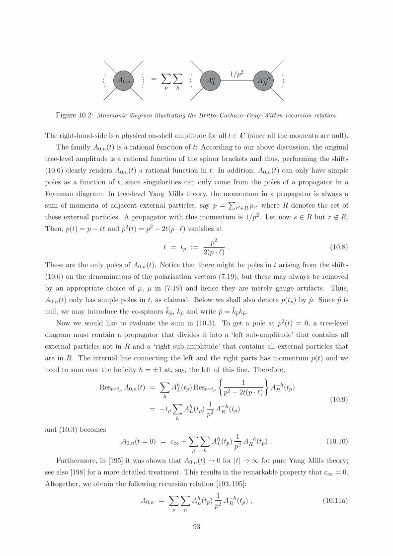
A0,n =∑
p
∑
h
AhL A−hR
1/p2
Figure 10.2: Mnemonic diagram illustrating the Britto–Cachazo–Feng–Witten recursion relation.
The right-hand-side is a physical on-shell amplitude for all t ∈ C (since all the momenta are null).
The family A0,n(t) is a rational function of t: According to our above discussion, the original
tree-level amplitude is a rational function of the spinor brackets and thus, performing the shifts
(10.6) clearly renders A0,n(t) a rational function in t. In addition, A0,n(t) can only have simple
poles as a function of t, since singularities can only come from the poles of a propagator in a
Feynman diagram: In tree-level Yang–Mills theory, the momentum in a propagator is always a
sum of momenta of adjacent external particles, say p =∑
r′∈R pr′ where R denotes the set of
these external particles. A propagator with this momentum is 1/p2. Let now s ∈ R but r 6∈ R.Then, p(t) = p− tℓ and p2(t) = p2 − 2t(p · ℓ) vanishes at
t = tp :=p2
2(p · ℓ) . (10.8)
These are the only poles of A0,n(t). Notice that there might be poles in t arising from the shifts
(10.6) on the denominators of the polarisation vectors (7.19), but these may always be removed
by an appropriate choice of µ, µ in (7.19) and hence they are merely gauge artifacts. Thus,
A0,n(t) only has simple poles in t, as claimed. Below we shall also denote p(tp) by p. Since p is
null, we may introduce the co-spinors kp, kp and write p = kpkp.
Now we would like to evaluate the sum in (10.3). To get a pole at p2(t) = 0, a tree-level
diagram must contain a propagator that divides it into a ‘left sub-amplitude’ that contains all
external particles not in R and a ‘right sub-amplitude’ that contains all external particles that
are in R. The internal line connecting the left and the right parts has momentum p(t) and we
need to sum over the helicity h = ±1 at, say, the left of this line. Therefore,
Rest=tp A0,n(t) =∑
h
AhL(tp)Rest=tp
1
p2 − 2t(p · ℓ)
A−hR (tp)
= −tp∑
h
AhL(tp)1
p2A−hR (tp)
(10.9)
and (10.3) becomes
A0,n(t = 0) = c∞ +∑
p
∑
h
AhL(tp)1
p2A−hR (tp) . (10.10)
Furthermore, in [195] it was shown that A0,n(t)→ 0 for |t| → ∞ for pure Yang–Mills theory;
see also [198] for a more detailed treatment. This results in the remarkable property that c∞ = 0.
Altogether, we obtain the following recursion relation [193,195]:
A0,n =∑
p
∑
h
AhL(tp)1
p2A−hR (tp) , (10.11a)
93
which is depicted in Figure 10.2. Here,
AhL(tp) = AhL(. . . , pr−1, pr, pr+1, . . .︸ ︷︷ ︸
6∈R
, p) ,
A−hR (tp) = A−h
R (−p, . . . , ps−1, ps, ps+1, . . .︸ ︷︷ ︸
∈R
) ,(10.11b)
where pr := pr(tp) and ps := ps(tp), respectively. Note that ultimately (10.11) tells us that
every scattering amplitude reduces to a sum of products of MHV and MHV amplitudes. This is
exemplified in the exercise below.
Exercise 10.1. Consider the MHV amplitude
AMHVn,0 (1+, r+) = gn−2
YM (2π)4δ(4)
(∑
r′
kr′kr′
)
[1r]4
[12] · · · [n1] .
Assume that this formula (and the one for the MHV amplitude) is valid up to n gluons. Use
the above recursion relation to prove its validity for n + 1 gluons by appropriately shifting
two of the co-spinors. Note that you will need to use both, MHV and MHV amplitudes as
left and right sub-amplitudes entering the recursion relation.
10.2. Recursion relations in maximally supersymmetric Yang–Mills theory
Finally, we would like to extend the above recursion relation to theN = 4 supersymmetric setting.
In Section 9.4., we saw that all the different scattering amplitudes inN = 4 supersymmetric Yang–
Mills theory are best understood when formulated in terms of superamplitudes or generating
functions F . In order to formulate a supersymmetric version of the recursion relation for the
tree-level superamplitudes F0,n, we follow [142,154,196]33 and consider the shifts
krA(t) := krA + tksA and ksα(t) := ksα − tkrα , (10.12)
with krα and ksA unshifted. Indeed, this is a direct supersymmetric extension of (10.6).
The supersymmetric recursion relations then follow from arguments similar to those which
led to (10.11). We therefore just record the result here [154]:
F0,n =∑
p
∫
d4ψp FL(tp)1
p2FR(tp) . (10.13)
Here, the ψip are the fermionic variables associated with the internal on-shell line with momentum
p. Notice that the sum over helicities gets replaced by the integral over the fermionic coordinates:
The superamplitudes FL and FR carry total helicities of −nL− 1 and −nR− 1 where nL and nR
are the number of external states on the left and right sub-amplitudes; see also Section 8.1. Since
the measure d4ψp carries a helicity of +2 (remember that each ψip carries a helicity of −1/2), the33See also Arkani-Hamed’s talk at “Wonders of Gauge Theory and Supergravity”, Paris 2008.
94

total helicity carried by the right-hand-side of (10.13) is −nL−nR and since F0,n has helicity −nwe have n = nL + nR as it should be.
In order to derive the recursion relations (10.13), one needs to verify that the one-parameter
family F0,n(t) of superamplitudes induced by (10.12) vanishes as |t| → ∞. This was explicitly
shown in [154] (see also [199, 142] for an earlier account). In fact, as proved by Arkani-Hamed,
Cachazo & Kaplan in [196], any N = 4 superamplitude behaves as34
Fn,0(t) → t−1 for |t| → ∞ . (10.14)
In the pure Yang–Mills setting, we have seen that the recursion relations imply that all
amplitudes are given in terms of MHV and MHV amplitudes. Likewise, (10.13) implies that
every superamplitude is given in terms of MHV and MHV superamplitudes. So far, we have
only given the MHV superamplitudes (8.17) explicitly. Therefore, in order to use (10.13) we also
need the MHV superamplitudes. Working—for a moment—in Minkowski signature, the MHV
superamplitudes are obtained from (8.17) via complex conjugation; see also Remark 8.1. Thus,
we may write
FMHV0,n = gn−2
YM (2π)4δ(4|0)(
n∑
r=1
krαkrβ
)
δ(0|8)(
n∑
r=1
ψrikrα
)
1
〈12〉〈23〉 · · · 〈n1〉 , (10.15)
where we have used kα = ikα. This, however, is not yet quite the form of the MHV superamp-
litudes that is suitable for the recursion relations as the left and right sub-amplitudes entering
(10.13) are holomorphic in the fermionic coordinates. To get an expression which depends holo-
morphically on the fermionic coordinates, we simply perform a Fourier transform on all the ψri
in (10.15) (see [171,105,155,118] for general amplitudes), that is,
FMHV0,n =
∫(
n∏
r=1
d4ψr
)
e−i∑n
r=1 ψriψir FMHV
0,n . (10.16)
Using the identity (8.18), we straightforwardly find (see also the exercise below) [118]
FMHV0,n =
gn−2YM
16(2π)4δ(4|0)
(n∑
r=1
krαkrβ
)
4∏
i=1
n∑
r,s=1
〈rs〉 ∂2
∂ψir∂ψis
n∏
r′=1
ψir′
1
〈12〉 · · · 〈n1〉 . (10.17)
We may now return to the complex setting by analytically continuing this expression, i.e. all
the kr, kr and ψir are to be regarded as complex. We have thus found a formula for the MHV
superamplitudes which depends holomorphically on the fermionic coordinates and which can
therefore be used in the supersymmetric recursion relations (10.13). A special case of (10.17) is
the three-particle MHV superamplitude [154]
FMHV0,3 = gYM(2π)4
δ(4|0)(p1 + p2 + p3)δ(0|4) (ψ1〈23〉+ ψ2〈31〉 + ψ3〈12〉)〈12〉〈23〉〈31〉 . (10.18)
34As also shown in [196], all superamplitudes in N = 8 supergravity behave as t−2 implying similar recursion
relations for maximal supergravity. See [200–202,142] for an earlier account of gravity recursion relations.
95

Exercise 10.2. Verify (10.17) and (10.18).
We have now provided all the necessary ingredients to construct general superamplitudes
from the MHV and MHV superamplitudes. In fact, the recursion relation generates all the tree-
level amplitudes from the three-particle amplitudes FMHV0,3 and FMHV
0,3 . The interested reader
might wish to consult the cited references (see e.g. [154, 196]) for explicit examples. Notice that
the three-particle amplitudes just follow from helicity information and Lorentz invariance and
without actually refering to a Lagrangian [203].
Remark 10.1. The Britto–Cachazo–Feng–Witten recursion relations have also been in-
vestigated from the point of view of twistor theory. The first twistor formulation of these
recursion relations was given in terms of twistor diagrams by Hodges in [173, 174, 204].
The Hodges construction is an ambidextrous approach as it uses both twistors and dual
twistors. This approach has been re-considered by Arkani-Hamed, Cachazo, Cheung & Ka-
plan in [175]. Mason & Skinner [106] discuss the recursion relations in terms of twistors
only. In particular, if we let W [F0,n](ZI1 , . . . , Z
In) be the Witten transform (8.43) of any
tree-level n-particle superamplitude F0,n (in Kleinian signature) where ZIr := (zAr , λrα) is
the supertwistor corresponding to particle r, then the shift (10.12) with r = 1 and s = n
corresponds to the simple shift W [F0,n](ZI1 , . . . , Z
In)→ W [F0,n](Z
I1 , . . . , Z
In−tZI1 ). See [106]
for more details.
96

Appendices

The main purpose of the subsequent appendices is to give an overview of some of the mathematical
concepts underlying these lecture notes that the reader might not be so familiar with. For obvious
reasons, it is impossible to give full-length explanations here. For a detailed account of the
following material, we refer to the literature cited at the beginning of these notes.
A. Vector bundles
Let X be a manifold (either smooth or complex). A complex rank-r vector bundle over X is
defined to be a manifold E together with a mapping π,
π : E → X , (A.1)
such that the following is fulfilled:
(V1) π is surjective,
(V2) for all x ∈ X, Ex := π−1(x) is a complex vector space of dimension r, i.e. there exists an
isomorphism hx : Ex → Cr(V3) and for all x ∈ X there exists a neighbourhood U ∋ x and a diffeomorphism hU : U×Cr →
π−1(U) such that π hU : U ×Cr → U with (x, v) 7→ x for any v ∈ Cr.The manifold E is called total space and Ex is the fibre over x ∈ X. Because of (V3), E is said
to be locally trivial and hU is called a trivialisation of E over U ⊂ X. A trivial vector bundle E
is globally of this form, i.e. E ∼= X ×Cr. A map s : X → E satisfying π s = idX is called a
section section of E. Notice that we could replace Cr in the above definition by Rr in which case
one speaks of real vector bundles of real rank r.
A useful description of vector bundles is in terms of transition functions. Let E → X be
a complex vector bundle and Ui be a covering of X with trivialisations hi : Ui × Cr →π−1(Ui) of E over Ui. If Ui ∩ Uj 6= ∅ then the functions fij := h−1
i hj : Ui ∩ Uj × Cr →Ui ∩ Uj ×Cr are called transition functions with respect to the covering. By definition, they are
diffeomorphisms. Furthermore, they define maps fij : Ui∩Uj → GL(r,C) via fij(x, v) = (x, fijv).
In the following, we shall not make a notational distinction between fij and fij and simply write
fij. By construction, the transition functions obey
fii = 1 on Ui , fij = f−1ji on Ui∩Uj 6= ∅ , fij fjk = fik on Ui∩Uj∩Uk 6= ∅ . (A.2)
The last of these equations is called the cocycle condition. Conversely, given a collection of
functions fij which obey (A.2), then one can construct a vector bundle such that the fij are its
transition functions. See e.g. [4] for a proof. So far, we have talked about complex vector bundles.
Likewise, one has holomorphic vector bundles E → X where X is a complex manifold and the
transition functions of E are assumed to be bi-holomorphic.
Let E and E′ be two vector bundles over X. A morphism (bundle map) φ : E → E′ is a
mapping such that φ restricted to the fibre Ex is a linear mapping to the fibre E′x for all x ∈ X.
98

We call φ a monomorphism if it is one-to-one on the fibres, an epimorphism if it is surjective on
the fibres and an isomorphism if it is one-to-one and surjective on the fibres. The vector bundle
E is a subbundle of E′ if E is a submanifold of E′ and Ex is a linear subspace of E′x for all x ∈ X.
An important concept we use throughout these notes is that of a pull-back. Let E → X be a
complex vector bundle and g : Y → X be a smooth mapping, then the pull-back bundle g∗E is
a complex vector bundle over Y of the same rank as E such that
g∗E −−−−→ Ey
y
Y −−−−→ X
(A.3)
is commutative. Put differently, the fibre of g∗E over y ∈ Y is just a copy of the fibre of E over
g(y) ∈ X. Furthermore, if Ui is a covering of X and fij are the transition functions of E then
g−1(Ui) defines a covering of Y such that g∗E is locally trivial. The transition functions g∗fij
of the pull-back bundle g∗E are then given by g∗fij = fij g.Moreover, given two complex vector bundles E and E′ over X, we can form new vector
bundles. For instance, we can form the dual vector bundles, the direct sum of E and E′, the
tensor product of E and E′, the symmetric tensor product of E and E′, which we respectively
denote by
E∗ , E ⊕ E′ , E ⊗ E′ , E ⊙ E′ , (A.4)
or if E is a subbundle of E′, one can form the quotient bundle E′/E. We can also form the
exterior product of a vector bundle
ΛkE , for k = 0, . . . , rankE . (A.5)
In each case, one defines the derived bundles fibrewise by the linear algebra operation indicated.
For example, the fibres of E ⊕ E′ are defined by (E ⊕ E′)x := Ex ⊕ E′x for all x ∈ X. If
r = rankE then ΛrE is given a special symbol detE and called the determinant line bundle since
the transition functions of ΛrE are given by the determinants of the transition functions of E.
In the case where E is the cotangent bundle T ∗X for some manifold X, detT ∗X is called the
canonical bundle and denoted by K or KX , respectively.
Another important concept is that of exact sequences. Let E1, E2 and E3 be three complex
vector bundles over X. Then the sequence
E1φ−→ E2
ψ−→ E3 (A.6)
is exact at E2 if kerψ = imφ. A short exact sequence is a sequence of the form
0 −→ E1 −→ E2 −→ E3 −→ 0 (A.7)
which is exact at E1, E2 and E3. We say that the sequence splits if E2∼= E1 ⊕ E3. Hence, one
can understand E2 in (A.7) as a deformation of the direct sum E1 ⊕ E3.
99
Let us give an example. Let X = CPm. Then0 −→ C φ−→ O(1)⊗Cm+1 ψ−→ TCPm −→ 0 (A.8)
is a short exact sequence which is called the Euler sequence (see also Remark 5.4.). This can
be understood as follows. Let π : Cm+1 \ 0 → CPm be the canonical projection and let za,
for a = 0, . . . ,m, be linear coordinates on Cm+1 (or equivalently, homogeneous coordinates onCPm). In Remark 4.2. we saw that π∗(za∂a) = 0, where ∂a := ∂/∂za. If we let s = (s0, . . . , sm)
be a section of O(1) ⊗ Cm+1, then the mapping ψ in (A.8) is given by ψ(s) = π∗(sa(z)∂a).
Clearly, ψ is surjective and moreover, its kernel is the trivial line bundle spanned by the section
s0 = (z0, . . . , zm), i.e. ψ(s0) = 0. Thus, (A.8) is indeed a short exact sequence as claimed.
The next concept we need is that of connections and curvature. Let E → X be a rank-r
complex vector bundle and let Ωp(X,E) be the differential p-forms on X with values in E. A
connection ∇ on E is a differential operator
∇ : Ωp(X,E) → Ωp+1(X,E) (A.9)
which obeys the Leibniz rule: For f some function on X and s a section of T pX ⊗ E, we have
∇(fs) = df ∧ s+ f∇s . (A.10)
Suppose now that e = e1, . . . , er is a local frame field of E over U ⊂ X, i.e. the ea are sections
of E over U , for a = 1, . . . , r, and for all x ∈ U , e1(x), . . . , er(x) is a basis for Ex. Then we may
introduce the connection one-form (or also referred to as the gauge potential) A according to
∇ea = Aabeb , (A.11)
i.e. A is a differential one-form with values in the endomorphism bundle EndE ∼= E∗ ⊗ E of E.
Thus, ∇ is locally of the form ∇ = d + A. Let Ui be a covering of X which trivialises E and
let ei := e|Ui= e1|Ui
, . . . , er|Ui be the frame field with respect to Ui. On Ui ∩Uj 6= ∅ we have
ei = fijej , where the fij are the transition functions of E. Upon substituting this into (A.11), we
find
Aj = f−1ij dfij + f−1
ij Aifij , with Ai := A|Ui. (A.12)
Hence, patching together the Ai according to this formula, we obtain a globally defined connection
one-form A. The curvature (also referred to as the field strength) of ∇ is defined as
F := ∇2 (A.13)
and is a section of Λ2T ∗X ⊗ EndE, i.e. under a change of trivialisation, F behaves as
Fj = f−1ij Fifij , with Fi := F |Ui
. (A.14)
Furthermore, the curvature is locally of the form
F = dA+A ∧A . (A.15)
Notice that ∇F = 0, which is the so-called Bianchi identity.
100

B. Characteristic classes
In this section, we shall define certain characteristic classes. However, we shall avoid the general
definition in terms of invariant polynomials and cohomology classes and instead focus on the
example of Chern classes and characters.
Let E → X be a complex vector bundle and F be the curvature two-form of a conncection
∇ = d +A on E. The total Chern class c(E) of E is defined by
c(E) := det
(
1 +i
2πF
)
. (B.1)
Since F is a differential two-form, c(E) is a sum of forms of even degrees. The Chern classes
ck(E) are defined by the expansion
c(E) = 1 + c1(E) + c2(E) + · · · . (B.2)
Notice that one should be more precise here, since the ck(E) written here are actually the Chern
forms: They are even differential forms which are closed. The Chern classes are defined as the
cohomology classes of the Chern forms and so the Chern forms are representatives of the Chern
classes. However, we shall loosely refer to the ck(E) as Chern classes, i.e. ck(E) ∈ H2k(X,Z)(see also Section 2.2. for the definition of the cohomology groups). Notice also that the above
definitions do not depend on the choice of connection. If E = TX then one usually writes ck(X).
If 2k > dimRX then ck(E) = 0. Furthermore, if k > rankE then ck(E) = 0, as well. Hence,
if E is a line bundle then c(E) = 1+c1(E) and if in addition c1(E) = 0 then E is a trivial bundle.
A few explicit Chern classes are
c0(E) = 1 ,
c1(E) =i
2πtrF ,
c2(E) =1
2
(i
2π
)2
[trF ∧ trF − tr (F ∧ F )] ,
...
cr(E) =
(i
2π
)r
detF ,
(B.3)
where r = rankE.
If we consider the direct sum E1 ⊕ E2 then c(E1 ⊕ E2) = c(E1) ∧ c(E2) as follows from the
properties of the determinant. Furthermore, this property is deformation independent, i.e. it
is also valid for the short exact sequence (A.7). This is known as the splitting principle. An
immediate consequence is then that c1(E1 ⊕ E2) = c1(E1) + c1(E2). This is an important fact
that we used in Section 5.2. when talking about Calabi–Yau spaces. Finally, if g∗E denotes
the pull-back bundle of E via some map g then c(g∗E) = g∗c(E). This is called naturality or
functoriality (see below).
A related quantity is the total Chern character. It is defined by
ch(E) := tr exp
(i
2πF
)
= ch0(E) + ch1(E) + ch2(E) + · · · . (B.4)
101
where the k-th Chern character is
chk(E) =1
k!tr
(i
2πF
)k
. (B.5)
The Chern characters can be expressed in terms of the Chern classes according to
ch0(E) = rankE ,
ch1(E) = c1(E) ,
ch2(E) =1
2[c1(E) ∧ c1(E)− 2c2(E)] ,
...
(B.6)
The total Chern character has the following properties. Let E1 and E2 be two complex vector
bundles. Then ch(E1 ⊕ E2) = ch(E1) + ch(E2) and ch(E1 ⊗ E2) = ch(E1) ∧ ch(E2). If g∗E
denotes the pull-back bundle of E via g then ch(g∗E) = g∗ch(E) which is also called naturality
or functoriality (see below).
Likewise, we may introduce Chern classes and characters for supervector bundles over super-
manifolds. Given a rank-r|s complex vector bundle E over a complex supermanifold X, we define
the k-th Chern class of E to be
ck(E) :=1
k!
dk
dtk
∣∣∣∣t=0
sdet
(
1 + ti
2πF
)
for k ≤ r + s , (B.7)
where F is again the curvature two-form of a connection∇ on E and ‘sdet’ is the superdeterminant
defined in (4.9). The first few Chern classes are given by:
c0(E) = 1 ,
c1(E) =i
2πstrF ,
c2(E) =1
2
(i
2π
)2
[strF ∧ strF − str (F ∧ F )] ,
...
(B.8)
Here, ‘str’ is the supertrace defined in (4.8). The total Chern class is then c(E) :=∑r+s
k=0 ck(E).
In a similar fashion, we may also introduce the k-th Chern character according to
chk(E) :=dk
dtk
∣∣∣∣t=0
str exp
(
ti
2πF
)
for k ≤ r + s . (B.9)
More details can be found, e.g. in the book by Bartocci et al. [19].
102

C. Categories
A category C consists of the following data:
(C1) a collection Ob(C ) of objects,
(C2) sets Mor(X,Y ) of morphisms for each pairX,Y ∈ Ob(C ), including a distinguished identity
morphism id = idX ∈Mor(X,X) for each X,
(C3) a composition of morphisms function : Mor(X,Y ) ×Mor(Y,Z) → Mor(X,Z) for each
triple X,Y,Z ∈ Ob(C ) satisfying f id = f = id f and (f g) h = f (g h).
There are many examples of categories, such as:
(i) The category of vector spaces over R or C consists of all vector spaces over R or C (=
objects). The morphisms are linear maps.
(ii) The category of topological spaces consists of all topological spaces (= objects). The morph-
isms are continuous maps.
(iii) The category of Ck-manifolds consists of all Ck-manifolds (= objects). The morphisms are
Ck-maps. Notice that k can also be infinity in which case one speaks of smooth manifolds.
(iv) The category of complex manifolds consists of all complex manifolds (= objects). The
morphisms are holomorphic maps.
(v) The categories of complex/holomorphic vector bundles consist of all complex/holomorphic
vector bundles (= objects). The morphisms are the smooth/holomorphic bundle maps.
(vi) The category of Lie algebras over R or C consists of all Lie algebras over R or C (= objects)
and the morphisms are those linear maps respecting the Lie bracket.
(vii) The category of Lie groups consists of all Lie groups (= objects). The morphisms are the
Lie morphisms, which are smooth group morphisms.
Besides the notion of categories, we need so-called functors which relate different categories.
A functor F from a category C to another category D takes each object X in Ob(C ) and assigns
an object F (X) in Ob(D) to it. Similarly, it takes each morphism f in Mor(X,Y ) and assigns
a morphism F (f) in Mor(F (X), F (Y )) to it such that F (id) = id and F (f g) = F (f) F (g).Pictorially, we have
Xf−−−−→ Y
F
y
yF
F (X) −−−−→F (f)
F (Y )
(C.1)
What we have just defined is a covariant functor. A contravariant functor differs from the
covariant functor by taking f in Mor(X,Y ) and assigning the morphism F (f) in Mor(F (Y ), F (X))
to it with F (id) = id and F (f g) = F (g) F (f).The standard example is the so-called dual vector space functor. This functor takes a vector
space V over R or C and assigns a dual vector space F (V ) = V ∗ to it and to each linear map
103

f : V →W it assigns the dual map F (f) = f∗ : W ∗ → V ∗, with ω 7→ ω f and ω ∈W ∗, in the
reverse direction. Hence, it is a contravariant functor.
Another functor we have already encountered is the parity map Π defined in (4.4), which is
a functor from the category of R-modules to the category of R-modules for R being a super-
commutative ring. To understand how it acts, let us take a closer look to morphisms between
R-modules. An additive mapping of R-modules, f : M → N , is called an even morphism if it
preserves the grading and is R-linear. We denote the group of such morphisms by Hom0(M,N).
On the other hand, we call an additive mapping of R-modules odd if it reverses the grading,
pf(m) = pm+1, and is R-linear, that is, f(rm) = (−)prrf(m) and f(mr) = f(m)r. The group of
such morphisms is denoted by Hom1(M,N). Then we set
Hom(M,N) := Hom0(M,N) ⊕Hom1(M,N) (C.2)
and it can be given an R-module structure. Then Π is defined in (4.4), where we implicitly
assumed that i) addition in ΠM is the same as in M , ii) right multiplication by R is the same
as in M and iii) left multiplication differs by a sign, i.e. rΠ(m) = (−)prΠ(rm) for r ∈ R, m ∈Mand Π(m) ∈ ΠM . Corresponding to the morphism f : M → N , we let fΠ : ΠM → ΠN be the
morphism which agrees with f as a mapping of sets. Moreover, corresponding to the morphism
f : M → N , we can find morphisms
Πf : M → ΠN , with (Πf)(m) := Π(f(m)) ,
fΠ : ΠM → N , with (fΠ)(Πm) := f(m) ,(C.3)
and hence fΠ = ΠfΠ. Therefore, Π is a covariant functor.
D. Sheaves
Let X be a topological space. A pre-sheaf S of Abelian groups on X consists of the following
data:
(P1) for all open subsets U ⊂ X, an Abelian group S(U) and
(P2) for all inclusions V ⊂ U of open subsets of X, a morphism of Abelian groups rUV : S(U)→S(V )
subject to the conditions:
(P3) r(∅) = 0,
(P4) rUU = idU : S(U)→ S(U) and
(P5) W ⊂ V ⊂ U , then rUV rVW = rUW .
Put differently, a pre-sheaf is just a contravariant functor from the category Top(X) (objects =
open sets of X, morphisms = inclusion maps) to the category Ab of Abelian groups. In fact, we
can replace Ab by any other fixed category C . Let S be a pre-sheaf on X, then S(U) are the
sections of S over U . The rUV are called restriction maps.
A pre-sheaf S on a topological space is a sheaf if it satisfies:
104
(S1) U open, Va open covering of U , s ∈ S(U) such that rUVa(s) = 0 for all a, then s = 0,
(S2) U open, Va open covering of U , sa ∈ S(Va), with rUVa∩Vb(sa) = rUVa∩Vb(sb), then there
exists an s ∈ S(U) such that rUVa(s) = sa for all a.
Point (S1) says that any section is determined by its local behaviour while (S2) means that local
sections can be pieced together to give global sections.
Examples are:
(i) Let X be a real manifold and U ⊂ X. Then S(U) := smooth functions on U, Ωp(U) :=
smooth p-forms on U, etc. are pre-sheaves, where the restriction mappings are the usual
restriction mappings. They are also sheaves.
(ii) Let X be a complex manifold and U ⊂ X. Then O(U) := holomorphic functions on U,Ωp,q(U) := smooth (p, q)-forms on U, etc. are pre-sheaves, where the restriction map-
pings are the usual restriction mappings. They are also sheaves.
(iii) Let E → X be a complex vector bundle over some manifold X and U ⊂ X. Then
S(E)(U) := smooth sections of E on U is a pre-sheaf, where the restriction mappings
are the usual restriction mappings. It is also a sheaf.
(iv) Let E → X be a holomorphic vector bundle over some complex manifold X and U ⊂ X.
Then O(E)(U) := holomorphic sections of E on U is a pre-sheaf, where the restriction
mappings are the usual restriction mappings. It is also a sheaf.
(v) Let R be a ring, X a topological space and U ⊂ X. Then R(U) is the ring of locally
constant continuous functions on U . This determines a pre-sheaf that is a sheaf. We call
this the constant sheaf R on X, e.g., R = R,C, . . ..(vi) Consider B(U) := bounded holomorphic functions on U ⊂ C. Then U → B(U) is a
pre-sheaf but not a sheaf.
The remainder of this appendix collects some basic notions regarding (pre-)sheaves. Firstly,
we need the notion of morphisms between (pre-)sheaves. A morphism of (pre-)sheaves φ : S → S ′
consists of a morphism of Abelian groups φU : S(U) → S ′(U) for all open subsets U such that
whenever V → U is an inclusion, the diagram
S(U)φU−−−−→ S ′(U)
rUV
y
yr′
UV
S(V ) −−−−→φV
S ′(V )
(D.1)
is commutative. An isomorphism is a morphism that has a two-sided inverse. A typical example
is the de Rham complex on a real manifold, where the sheaf morphism is the usual exterior
derivative.
Let S be a pre-sheaf and
Sx :=⋃
U∋xS(U) . (D.2)
105
Then we say that two elements of Sx, f ∈ S(U), U ∋ x and g ∈ S(V ), V ∋ x, are equivalent if
there exists an open set W ⊂ (U ∩ V ), with x ∈W such that
rUW (f) = rVW (g) . (D.3)
We define the stalk Sx to be the set of equivalence classes induced by this equivalence relation.
Of course, Sx inherits the algebraic structure of the pre-sheaf S, i.e. we can add elements in Sxby adding representatives of equivalence classes. We shall let
π := rUx : S(U) → Sx (D.4)
be the natural restriction mapping to stalks.
Let φ : S → S ′ be a morphism of sheaves on a topological space X. Then φ is an isomorphism
if and only if the induced map on the stalks φx : Sx → S ′x is an isomorphism for all x ∈ X. Note
that this is not true for pre-sheaves.
Secondly, let us say a few words about exact sequences. We say that a sequence of morphisms
of sheaves
S1 φ−→ S2 ψ−→ S3 (D.5)
on a topological space X is exact at S2 if the induced sequence
S1x φx−→ S2x ψx−→ S3x (D.6)
is exact, i.e. kerψx = imφx for all x ∈ X. A short exact sequence of sheaves is a sequence of the
form
0 −→ S1 −→ S2 −→ S3 −→ 0 (D.7)
which is exact at S1, S2 and S3.Before moving on, let us pause and give an example. Let O∗ be the sheaf of non-vanishing
holomorphic functions on a complex manifold X. Then
0 −→ Z −→ O exp−→ O∗ −→ 0 (D.8)
is a short exact sequence, where exp(f) := e2πif ∈ O∗(U) for f ∈ O(U) with U ⊂ X. This
sequence is called the exponential sheaf sequence.
In Section 2.2., we introduced the notion of sheaf cohomology, so let us state a basic fact
about the sheaf cohomology for short exact sequences. Let X be a topological space together
with a short exact sequence of the form (D.7). Then (D.7) always induces a long exact sequence
of Cech cohomology groups according to:
0 −→ H0(X,S1) −→ H0(X,S2) −→ H0(X,S3)−→ H1(X,S1) −→ H1(X,S2) −→ H1(X,S3)
−→ H2(X,S1) −→ H2(X,S2) −→ H2(X,S3) −→ · · ·
(D.9)
For a proof, see e.g. [4, 9].
106

Let us come back to the exponential sheaf sequence. We have
· · · −→ H1(X,Z) −→ H1(X,O) exp−→ H1(X,O∗)c1−→ H2(X,Z) −→ · · · (D.10)
By virtue of our discussion in Section 5.2., H1(X,O∗) parametrises the holomorphic line bundles
E → X. The image c1(E) ∈ H2(X,Z) of a line bundle E ∈ H1(X,O∗) is the first Chern class. If
X = CPm then H1(CPm,O) = 0 = H2(CPm,O) and the above long exact cohomology sequence
yields H1(CPm,O∗) ∼= H2(CPm,Z) ∼= Z, i.e. we have a classification of all holomorphic line
bundles on complex projective space CPm. Another related example we already encountered is
given for the choice X = P 3 and E → P 3 a holomorphic line bundle over P 3. ThenH1(P 3,Z) = 0
since P 3 is simply connected and if in addition c1(E) = 0, i.e. E|Lx is holomorphically trivial on
any Lx → P 3, then we conclude from the above sequence that
H1(P 3,O) ∼= E ∈ H1(P 3,O∗) | c1(E) = 0 . (D.11)
This is basically the content of Exercise 3.3.
107

References
[1] L. J. Mason and N. M. J. Woodhouse, “Integrability, self-duality, and twistor theory”, Clarendon,
Oxford, 1996.
[2] M. Dunajski, “Solitons, instantons and twistors”, Oxford Univ. Pr., Oxford, 2009.
[3] H. B. Lawson Jr. and M. L. Michelsohn, “Spin geometry”, Princeton Univ. Pr., Princeton, 1989.
[4] R. S. Ward and R. O. Wells, “Twistor geometry and field theory”, Cambridge Univ. Pr.,
Cambridge, 1990.
[5] R. Penrose, “Twistor algebra”, J. Math. Phys. 8, 345 (1967).
[6] R. Penrose, “Solutions of the zero-rest-mass equations”, J. Math. Phys. 10, 38 (1969).
[7] R. Penrose, “The twistor program”, Rept. Math. Phys. 12, 65 (1977).
[8] J. Radon, “Uber die Bestimmung von Funktionen durch ihre Integralwerte langs gewisser
Mannigfaltigkeiten”, Ber. Verh. Sachs. Akad. Wiss. Leipzig, Math. Nat. 69, 262 (1917).
[9] P. Griffiths and J. Harris, “Principles of algebraic geometry”, John Wiley & Sons, New York, 1978.
[10] F. Hirzebruch, “Topological methods in algebraic geometry”, Springer Verlag, New York, 1966.
[11] D. Burns, “Some background and examples in deformation theory”, in: “Complex manifold
techniques in theoretical physics”, Eds. D. Lerner and P. Sommers, Pitman, San
Fransisco–London–Melbourne, 1979.
[12] K. Kodaira, “Complex manifolds and deformation of complex structures”, Springer Verlag, New
York, 1986.
[13] R. S. Ward, “On self-dual gauge fields”, Phys. Lett. A61, 81 (1977).
[14] L. Crane, “Action of the loop group on the self-dual Yang–Mills equation”,
Commun. Math. Phys. 110, 391 (1987).
[15] A. A. Belavin, A. M. Polyakov, A. S. Schwarz and Y. S. Tyupkin, “Pseudo-particle solutions of the
Yang–Mills equations”, Phys. Lett. B59, 85 (1975).
[16] M. K. Prasad, “Instantons and monopoles in Yang–Mills gauge field theories”,
Physica D1, 167 (1980).
[17] D. Tong, “TASI lectures on solitons: Instantons, monopoles, vortices and kinks”, hep-th/0509216,
Tasi Lecture, Boulder, 2005.
[18] Y. I. Manin, “Gauge field theory and complex geometry”, Springer Verlag, New York, 1988.
[19] C. Bartocci, U. Bruzzo and D. Hernandez-Ruiperez, “The geometry of supermanifolds”, Kluwer,
Dordrecht, 1991.
[20] B. S. DeWitt, “Supermanifolds”, Cambridge Univ. Pr., Cambridge, 1992.
[21] M. Batchelor, “The structure of supermanifolds”, Trans. Amer. Math. Soc. 253, 329 (1979).
[22] A. Ferber, “Supertwistors and conformal supersymmetry”, Nucl. Phys. B132, 55 (1978).
[23] T. N. Bailey and M. G. Eastwood, “Complex paraconformal manifolds - their differential geometry
and twistor theory”, Forum Math. 3, 61 (1991).
[24] L. Frappat, P. Sorba and A. Sciarrino, “Dictionary on Lie superalgebras”, hep-th/9607161.
[25] A. M. Semikhatov, “Supersymmetric instanton”, JETP Lett. 35, 560 (1982).
108
[26] I. V. Volovich, “Super-self-duality for supersymmetric Yang–Mills theory”,
Phys. Lett. B123, 329 (1983).
[27] J. P. Harnad, J. Hurtubise, M. Legare and S. Shnider, “Constraint equations and field equations in
supersymmetric N = 3 Yang–Mills theory”, Nucl. Phys. B256, 609 (1985).
[28] J. P. Harnad and S. Shnider, “Constraints and field equations for ten-dimensional super
Yang–Mills theory”, Commun. Math. Phys. 106, 183 (1986).
[29] C. Devchand and V. Ogievetsky, “Interacting fields of arbitrary spin and N > 4 supersymmetric
self-dual Yang–Mills equations”, Nucl. Phys. B481, 188 (1996), hep-th/9606027.
[30] W. Siegel, “The N = 2 (4) string is self-dual N = 4 Yang–Mills”, Phys. Rev. D46, 3235 (1992),
hep-th/9205075.
[31] K. Pohlmeyer, “On the Lagrangian theory of anti-(self)-dual fields in four-dimensional Euclidean
space”, Commun. Math. Phys. 72, 37 (1980).
[32] L.-L. Chau, M.-l. Ge and Y.-s. Wu, “The Kac–Moody algebra in the self-dual Yang–Mills
equation”, Phys. Rev. D25, 1086 (1982).
[33] L.-L. Chau and W. Yong-shi, “More about hidden symmetry algebra for the self-dual Yang–Mills
system”, Phys. Rev. D26, 3581 (1982).
[34] L.-L. Chau, M.-L. Ge, A. Sinha and Y.-S. Wu, “Hidden symmetry algebra for the self-dual
Yang–Mills equation”, Phys. Lett. B121, 391 (1983).
[35] K. Ueno and Y. Nakamura, “Transformation theory for anti-(self)-dual equations and the
Riemann–Hilbert problem”, Phys. Lett. B117, 208 (1982).
[36] L. Dolan, “A new symmetry group of real self-dual Yang–Mills”, Phys. Lett. B113, 387 (1982).
[37] L. Dolan, “Kac–Moody algebras and exact solvability in hadronic physics”,
Phys. Rept. 109, 1 (1984).
[38] A. D. Popov and C. R. Preitschopf, “Conformal symmetries of the self-dual Yang–Mills
equations”, Phys. Lett. B374, 71 (1996), hep-th/9512130.
[39] A. D. Popov, “Self-dual Yang–Mills: Symmetries and moduli space”,
Rev. Math. Phys. 11, 1091 (1999), hep-th/9803183.
[40] A. D. Popov, “Holomorphic Chern–Simons–Witten theory: From 2D to 4D conformal field
theories”, Nucl. Phys. B550, 585 (1999), hep-th/9806239.
[41] T. A. Ivanova, “On current algebra of symmetries of the self-dual Yang–Mills equations”,
J. Math. Phys. 39, 79 (1998), hep-th/9702144.
[42] M. Wolf, “On hidden symmetries of a super gauge theory and twistor string theory”,
JHEP 0502, 018 (2005), hep-th/0412163.
[43] M. Wolf, “Twistors and aspects of integrability of self-dual SYM theory”,
Proc. of the Intern. Workshop on Supersymmetries and Quantum Symmetries 1, 448 (2005),
hep-th/0511230.
[44] M. Wolf, “On supertwistor geometry and integrability in super gauge theory”, hep-th/0611013,
PhD thesis, Leibniz Universitat Hannover (2006).
[45] A. D. Popov and M. Wolf, “Hidden symmetries and integrable hierarchy of the N = 4
supersymmetric Yang–Mills equations”, Commun. Math. Phys. 275, 685 (2007), hep-th/0608225.
109

[46] W. A. Bardeen, “Self-dual Yang–Mills theory, integrability and multiparton amplitudes”,
Prog. Theor. Phys. Suppl. 123, 1 (1996).
[47] D. Cangemi, “Self-dual Yang–Mills theory and one-loop maximally helicity violating multi-gluon
amplitudes”, Nucl. Phys. B484, 521 (1997), hep-th/9605208.
[48] D. Cangemi, “Self-duality and maximally helicity violating QCD amplitudes”,
Int. J. Mod. Phys. A12, 1215 (1997), hep-th/9610021.
[49] A. A. Rosly and K. G. Selivanov, “On amplitudes in self-dual sector of Yang–Mills theory”,
Phys. Lett. B399, 135 (1997), hep-th/9611101.
[50] E. Witten, “Chern–Simons gauge theory as a string theory”, Prog. Math. 133, 637 (1995),
hep-th/9207094.
[51] V. Bouchard, “Lectures on complex geometry, Calabi–Yau manifolds and toric geometry”,
hep-th/0702063.
[52] S. Sethi, “Supermanifolds, rigid manifolds and mirror symmetry”, Nucl. Phys. B430, 31 (1994),
hep-th/9404186.
[53] E. Witten, “Perturbative gauge theory as a string theory in twistor space”,
Commun. Math. Phys. 252, 189 (2004), hep-th/0312171.
[54] M. Rocek and N. Wadhwa, “On Calabi–Yau supermanifolds”,
Adv. Theor. Math. Phys. 9, 315 (2005), hep-th/0408188.
[55] C.-G. Zhou, “On Ricci-flat supermanifolds”, JHEP 0502, 004 (2005), hep-th/0410047.
[56] M. Rocek and N. Wadhwa, “On Calabi–Yau supermanifolds. II”, hep-th/0410081.
[57] C. Samann, “The topological B model on fattened complex manifolds and subsectors of N = 4
self-dual Yang–Mills theory”, JHEP 0501, 042 (2005), hep-th/0410292.
[58] U. Lindstrom, M. Rocek and R. von Unge, “Ricci-flat supertwistor spaces”,
JHEP 0601, 163 (2006), hep-th/0509211.
[59] R. Ricci, “Super Calabi–Yau’s and special Lagrangians”, JHEP 0703, 048 (2007), hep-th/0511284.
[60] C. R. LeBrun, “Geometry of twistor spaces”, Simons Workshop Lecture, Stony Brook, 2004.
[61] E. Sokatchev, “An action for N = 4 supersymmetric self-dual Yang–Mills theory”,
Phys. Rev. D53, 2062 (1996), hep-th/9509099.
[62] A. D. Popov, “Hermitian Yang–Mills equations and pseudo-holomorphic bundles on nearly Kahler
and nearly Calabi–Yau twistor 6-manifolds”, Nucl. Phys. B828, 594 (2010), arxiv:0907.0106.
[63] S. Karnas and S. V. Ketov, “An action of N = 8 self-dual supergravity in ultra-hyperbolic
harmonic superspace”, Nucl. Phys. B526, 597 (1998), hep-th/9712151.
[64] L. J. Mason and M. Wolf, “Twistor actions for self-dual supergravities”,
Commun. Math. Phys. 288, 97 (2009), arxiv:0706.1941.
[65] A. D. Popov and C. Samann, “On supertwistors, the Penrose–Ward transform and N = 4 super
Yang–Mills theory”, Adv. Theor. Math. Phys. 9, 931 (2005), hep-th/0405123.
[66] L. J. Mason, “Twistor actions for non-self-dual fields: A derivation of twistor string theory”,
JHEP 0510, 009 (2005), hep-th/0507269.
[67] R. Boels, L. Mason and D. Skinner, “Supersymmetric gauge theories in twistor space”,
JHEP 0702, 014 (2007), hep-th/0604040.
110
[68] R. Boels, L. Mason and D. Skinner, “From twistor actions to MHV diagrams”,
Phys. Lett. B648, 90 (2007), hep-th/0702035.
[69] M. Nakahara, “Geometry, topology and physics”, The Institute of Physics, Bristol–Philadelphia,
2002.
[70] N. M. J. Woodhouse, “Real methods in twistor theory”, Class. Quant. Grav. 2, 257 (1985).
[71] A. D. Popov and M. Wolf, “Topological B model on weighted projective spaces and self-dual models
in four dimensions”, JHEP 0409, 007 (2004), hep-th/0406224.
[72] S. Giombi, M. Kulaxizi, R. Ricci, D. Robles-Llana, D. Trancanelli and K. Zoubos, “Orbifolding the
twistor string”, Nucl. Phys. B719, 234 (2005), hep-th/0411171.
[73] D.-W. Chiou, O. J. Ganor, Y. P. Hong, B. S. Kim and I. Mitra, “Massless and massive
three-dimensional super Yang–Mills theory and mini-twistor string theory”,
Phys. Rev. D71, 125016 (2005), hep-th/0502076.
[74] A. D. Popov, C. Samann and M. Wolf, “The topological B model on a mini-supertwistor space and
supersymmetric Bogomolny monopole equations”, JHEP 0510, 058 (2005), hep-th/0505161.
[75] O. Lechtenfeld and C. Samann, “Matrix models and D branes in twistor string theory”,
JHEP 0603, 002 (2006), hep-th/0511130.
[76] L. J. Mason and D. Skinner, “An ambitwistor Yang–Mills Lagrangian”,
Phys. Lett. B636, 60 (2006), hep-th/0510262.
[77] J. Bedford, C. Papageorgakis and K. Zoubos, “Twistor strings with flavour”,
JHEP 0711, 088 (2007), arxiv:0708.1248.
[78] R. A. Bertlmann, “Anomalies in quantum field theory”, Clarendon, Oxford, 1996.
[79] E. Witten, “An interpretation of classical Yang–Mills theory”, Phys. Lett. B77, 394 (1978).
[80] J. Isenberg, P. B. Yasskin and P. S. Green, “Non-self-dual gauge fields”,
Phys. Lett. B78, 462 (1978).
[81] M. G. Eastwood, “Supersymmetry, twistors, and the Yang–Mills equations”,
Trans. Amer. Math. Soc. 301, 615 (1987).
[82] J. P. Harnad, J. Hurtubise and S. Shnider, “Supersymmetric Yang–Mills equations and
supertwistors”, Ann. Phys. 193, 40 (1989).
[83] P. S. Howe and G. G. Hartwell, “A superspace survey”, Class. Quant. Grav. 12, 1823 (1995).
[84] C. Samann, “On the mini-superambitwistor space and N = 8 super Yang–Mills theory”,
Adv. Math. Phys. 2009, 784215 (2009), hep-th/0508137.
[85] K. Hori, S. Katz, A. Klemm, P. Rahul, R. Thomas, C. Vafa, R. Vakil and E. Zaslow, “Mirror
symmetry”, Amer. Math. Soc., Providence, 2003.
[86] N. Berkovits, “An alternative string theory in twistor space for N = 4 super Yang–Mills”,
Phys. Rev. Lett. 93, 011601 (2004), hep-th/0402045.
[87] L. Mason and D. Skinner, “Heterotic twistor string theory”, Nucl. Phys. B795, 105 (2008),
arxiv:0708.2276.
[88] N. Berkovits and E. Witten, “Conformal supergravity in twistor string theory”,
JHEP 0408, 009 (2004), hep-th/0406051.
111
[89] R. Kleiss and H. Kuijf, “Multi-gluon cross-sections and five-jet production at hadron colliders”,
Nucl. Phys. B312, 616 (1989).
[90] M. L. Mangano and S. J. Parke, “Multi-parton amplitudes in gauge theories”,
Phys. Rept. 200, 301 (1991), hep-th/0509223.
[91] S. J. Parke and T. R. Taylor, “An amplitude for n-gluon scattering”,
Phys. Rev. Lett. 56, 2459 (1986).
[92] F. A. Berends and W. T. Giele, “Recursive calculations for processes with n gluons”,
Nucl. Phys. B306, 759 (1988).
[93] M. T. Grisaru, H. N. Pendleton and P. van Nieuwenhuizen, “Supergravity and the S-matrix”,
Phys. Rev. D15, 996 (1977).
[94] M. T. Grisaru and H. N. Pendleton, “Some properties of scattering amplitudes in supersymmetric
theories”, Nucl. Phys. B124, 81 (1977).
[95] S. J. Parke and T. R. Taylor, “Perturbative QCD utilizing extended supersymmetry”,
Phys. Lett. B157, 81 (1985).
[96] Z. Kunszt, “Combined use of the CALKUL method and N = 1 supersymmetry to calculate QCD
six-parton processes”, Nucl. Phys. B271, 333 (1986).
[97] Z. Bern, L. J. Dixon, D. C. Dunbar and D. A. Kosower, “One-loop self-dual and N = 4 super
Yang-Mills”, Phys. Lett. B394, 105 (1997), hep-th/9611127.
[98] L. J. Dixon, “Calculating scattering amplitudes efficiently”, hep-ph/9601359, Tasi Lecture,
Boulder, 1995.
[99] Z. Bern and D. A. Kosower, “Color decomposition of one-loop amplitudes in gauge theories”,
Nucl. Phys. B362, 389 (1991).
[100] G. ’t Hooft, “A planar diagram theory for strong interactions”, Nucl. Phys. B72, 461 (1974).
[101] Z. Bern, L. J. Dixon, D. C. Dunbar and D. A. Kosower, “One-loop n-point gauge theory
amplitudes, unitarity and collinear limits”, Nucl. Phys. B425, 217 (1994), hep-ph/9403226.
[102] S. Weinberg, “The quantum theory of fields. Vol. 1: Foundations”, Cambridge Univ. Pr.,
Cambridge, 1995.
[103] F. A. Berends and W. Giele, “The six-gluon process as an example of Weyl–van der Waerden
spinor calculus”, Nucl. Phys. B294, 700 (1987).
[104] W. Siegel, “Fields”, hep-th/9912205.
[105] J. M. Drummond, J. Henn, G. P. Korchemsky and E. Sokatchev, “Dual superconformal symmetry
of scattering amplitudes in N = 4 super Yang–Mills theory”, Nucl. Phys. B828, 317 (2010),
arxiv:0807.1095.
[106] L. Mason and D. Skinner, “Scattering amplitudes and BCFW recursion in twistor space”,
arxiv:0903.2083.
[107] V. P. Nair, “A current algebra for some gauge theory amplitudes”, Phys. Lett. B214, 215 (1988).
[108] S. Mandelstam, “Light-cone superspace and the ultraviolet finiteness of the N = 4 model”,
Nucl. Phys. B213, 149 (1983).
[109] L. Brink, O. Lindgren and B. E. W. Nilsson, “N = 4 Yang–Mills theory on the light-cone”,
Nucl. Phys. B212, 401 (1983).
112
[110] F. Cachazo, P. Svrcek and E. Witten, “Gauge theory amplitudes in twistor space and holomorphic
anomaly”, JHEP 0410, 077 (2004), hep-th/0409245.
[111] T. Bargheer, N. Beisert, W. Galleas, F. Loebbert and T. McLoughlin, “Exacting N = 4
superconformal symmetry”, JHEP 0911, 056 (2009), arxiv:0905.3738.
[112] A. Sever and P. Vieira, “Symmetries of the N = 4 SYM S-matrix”, arxiv:0908.2437.
[113] G. P. Korchemsky and E. Sokatchev, “Symmetries and analytic properties of scattering amplitudes
in N = 4 SYM theory”, Nucl. Phys. B832, 1 (2010), arxiv:0906.1737.
[114] F. Cachazo, P. Svrcek and E. Witten, “MHV vertices and tree amplitudes in gauge theory”,
JHEP 0409, 006 (2004), hep-th/0403047.
[115] D. A. Kosower, “Next-to-maximal-helicity-violating amplitudes in gauge theory”,
Phys. Rev. D71, 045007 (2005), hep-th/0406175.
[116] I. Bena, Z. Bern and D. A. Kosower, “Twistor space recursive formulation of gauge theory
amplitudes”, Phys. Rev. D71, 045008 (2005), hep-th/0406133.
[117] K. Risager, “A direct proof of the CSW rules”, JHEP 0512, 003 (2005), hep-th/0508206.
[118] H. Elvang, D. Z. Freedman and M. Kiermaier, “Recursion relations, generating functions, and
unitarity sums in N = 4 SYM theory”, JHEP 0904, 009 (2009), arxiv:0808.1720.
[119] H. Elvang, D. Z. Freedman and M. Kiermaier, “Proof of the MHV vertex expansion for all tree
amplitudes in N = 4 SYM theory”, JHEP 0906, 068 (2009), arxiv:0811.3624.
[120] G. Georgiou, E. W. N. Glover and V. V. Khoze, “Non-MHV tree amplitudes in gauge theory”,
JHEP 0407, 048 (2004), hep-th/0407027.
[121] R. Boels, “A quantization of twistor Yang–Mills theory through the background field method”,
Phys. Rev. D76, 105027 (2007), hep-th/0703080.
[122] L. Mason and D. Skinner, “Gravity, Twistors and the MHV Formalism”,
Commun. Math. Phys. 294, 827 (2010), arxiv:0808.3907.
[123] S. Axelrod and I. M. Singer, “Chern-Simons perturbation theory”,
Proc. Diff. Geom. Meth. Theor. Phys. 1, 3 (1991), hep-th/9110056.
[124] S. Axelrod and I. M. Singer, “Chern-Simons perturbation theory. 2”,
J. Diff. Geom. 39, 173 (1994), hep-th/9304087.
[125] W. Jiang, “Yang–Mills theory in twistor space”, arxiv:0809.0328, PhD thesis, University of
Oxford (2008).
[126] A. Brandhuber, B. Spence and G. Travaglini, “Amplitudes in pure Yang–Mills and MHV
diagrams”, JHEP 0702, 088 (2007), hep-th/0612007.
[127] A. Brandhuber, B. Spence and G. Travaglini, “One-loop gauge theory amplitudes in N = 4 super
Yang–Mills from MHV vertices”, Nucl. Phys. B706, 150 (2005), hep-th/0407214.
[128] C. Quigley and M. Rozali, “One-loop MHV amplitudes in supersymmetric gauge theories”,
JHEP 0501, 053 (2005), hep-th/0410278.
[129] J. Bedford, A. Brandhuber, B. J. Spence and G. Travaglini, “A twistor approach to one-loop
amplitudes in N = 1 supersymmetric Yang–Mills theory”, Nucl. Phys. B706, 100 (2005),
hep-th/0410280.
113

[130] J. Bedford, A. Brandhuber, B. J. Spence and G. Travaglini, “Non-supersymmetric loop amplitudes
and MHV vertices”, Nucl. Phys. B712, 59 (2005), hep-th/0412108.
[131] E. W. N. Glover, P. Mastrolia and C. Williams, “One-loop phi-MHV amplitudes using the unitarity
bootstrap: The general helicity case”, JHEP 0808, 017 (2008), arxiv:0804.4149.
[132] R. Boels and C. Schwinn, “Deriving CSW rules for massive scalar legs and pure Yang–Mills
loops”, JHEP 0807, 007 (2008), arxiv:0805.1197.
[133] P. Mansfield, “The Lagrangian origin of MHV rules”, JHEP 0603, 037 (2006), hep-th/0511264.
[134] A. Gorsky and A. Rosly, “From Yang–Mills Lagrangian to MHV diagrams”,
JHEP 0601, 101 (2006), hep-th/0510111.
[135] J. H. Ettle and T. R. Morris, “Structure of the MHV rules Lagrangian”, JHEP 0608, 003 (2006),
hep-th/0605121.
[136] H. Feng and Y.-t. Huang, “MHV Lagrangian for N = 4 super Yang–Mills”,
JHEP 0904, 047 (2009), hep-th/0611164.
[137] J. H. Ettle, “MHV Lagrangians for Yang–Mills and QCD”, arxiv:0808.1973, PhD thesis,
University of Southampton (2008).
[138] S. Giombi, R. Ricci, D. Robles-Llana and D. Trancanelli, “A note on twistor gravity amplitudes”,
JHEP 0407, 059 (2004), hep-th/0405086.
[139] V. P. Nair, “A note on MHV amplitudes for gravitons”, Phys. Rev. D71, 121701 (2005),
hep-th/0501143.
[140] N. E. J. Bjerrum-Bohr, D. C. Dunbar, H. Ita, W. B. Perkins and K. Risager, “MHV vertices for
gravity amplitudes”, JHEP 0601, 009 (2006), hep-th/0509016.
[141] A. Nasti and G. Travaglini, “One-loop N = 8 supergravity amplitudes from MHV diagrams”,
Class. Quant. Grav. 24, 6071 (2007), arxiv:0706.0976.
[142] M. Bianchi, H. Elvang and D. Z. Freedman, “Generating tree amplitudes in N = 4 SYM and
N = 8 SG”, JHEP 0809, 063 (2008), arxiv:0805.0757.
[143] M. Wolf, “Self-dual supergravity and twistor theory”, Class. Quant. Grav. 24, 6287 (2007),
arxiv:0705.1422.
[144] M. Kiermaier and S. G. Naculich, “A super MHV vertex expansion for N = 4 SYM theory”,
JHEP 0905, 072 (2009), arxiv:0903.0377.
[145] J. M. Drummond and J. M. Henn, “All tree-level amplitudes in N = 4 SYM”,
JHEP 0904, 018 (2009), arxiv:0808.2475.
[146] J. M. Drummond, J. Henn, V. A. Smirnov and E. Sokatchev, “Magic identities for conformal
four-point integrals”, JHEP 0701, 064 (2007), hep-th/0607160.
[147] L. F. Alday and J. M. Maldacena, “Gluon scattering amplitudes at strong coupling”,
JHEP 0706, 064 (2007), arxiv:0705.0303.
[148] R. Ricci, A. A. Tseytlin and M. Wolf, “On T-duality and integrability for strings on AdS
backgrounds”, JHEP 0712, 082 (2007), arxiv:0711.0707.
[149] J. M. Drummond, G. P. Korchemsky and E. Sokatchev, “Conformal properties of four-gluon
planar amplitudes and Wilson loops”, Nucl. Phys. B795, 385 (2008), arxiv:0707.0243.
114

[150] L. F. Alday and J. Maldacena, “Comments on gluon scattering amplitudes via AdS/CFT”,
JHEP 0711, 068 (2007), arxiv:0710.1060.
[151] J. M. Drummond, J. Henn, G. P. Korchemsky and E. Sokatchev, “Conformal Ward identities for
Wilson loops and a test of the duality with gluon amplitudes”, Nucl. Phys. B826, 337 (2010),
arxiv:0712.1223.
[152] N. Berkovits and J. Maldacena, “Fermionic T-duality, dual superconformal symmetry, and the
amplitude/Wilson loop connection”, JHEP 0809, 062 (2008), arxiv:0807.3196.
[153] N. Beisert, R. Ricci, A. A. Tseytlin and M. Wolf, “Dual superconformal symmetry from AdS5 × S5
superstring integrability”, Phys. Rev. D78, 126004 (2008), arxiv:0807.3228.
[154] A. Brandhuber, P. Heslop and G. Travaglini, “A note on dual superconformal symmetry of the
N = 4 super Yang–Mills S-matrix”, Phys. Rev. D78, 125005 (2008), arxiv:0807.4097.
[155] J. M. Drummond, J. Henn, G. P. Korchemsky and E. Sokatchev, “Generalized unitarity for N = 4
superamplitudes”, arxiv:0808.0491.
[156] J. M. Drummond, J. M. Henn and J. Plefka, “Yangian symmetry of scattering amplitudes in
N = 4 super Yang–Mills theory”, JHEP 0905, 046 (2009), arxiv:0902.2987.
[157] N. Beisert, “T-Duality, dual conformal symmetry and integrability for strings on AdS5 × S5”,
Fortschr. Phys. 57, 329 (2009), arxiv:0903.0609.
[158] L. F. Alday, J. M. Henn, J. Plefka and T. Schuster, “Scattering into the fifth dimension of N = 4
super Yang–Mills”, JHEP 1001, 077 (2010), arxiv:0908.0684.
[159] J. M. Henn, S. G. Naculich, H. J. Schnitzer and M. Spradlin, “Higgs-regularized three-loop
four-gluon amplitude in N = 4 SYM: exponentiation and Regge limits”, JHEP 1004, 038 (2010),
arxiv:1001.1358.
[160] J. M. Drummond and L. Ferro, “Yangians, Grassmannians and T-duality”,
JHEP 1007, 027 (2010), arxiv:1001.3348.
[161] A. Hodges, “Eliminating spurious poles from gauge-theoretic amplitudes”, arxiv:0905.1473.
[162] N. Arkani-Hamed, F. Cachazo, C. Cheung and J. Kaplan, “A duality for the S-matrix”,
JHEP 1003, 020 (2010), arxiv:0907.5418.
[163] L. Mason and D. Skinner, “Dual superconformal invariance, momentum twistors and
Grassmannians”, JHEP 0911, 045 (2009), arxiv:0909.0250.
[164] N. Arkani-Hamed, F. Cachazo and C. Cheung, “The Grassmannian origin of dual superconformal
invariance”, JHEP 1003, 036 (2010), arxiv:0909.0483.
[165] N. Arkani-Hamed, J. Bourjaily, F. Cachazo and J. Trnka, “Unification of residues and
Grassmannian dualities”, arxiv:0912.4912.
[166] L. F. Alday and R. Roiban, “Scattering amplitudes, Wilson loops and the string/gauge theory
correspondence”, Phys. Rept. 468, 153 (2008), arxiv:0807.1889.
[167] J. M. Henn, “Duality between Wilson loops and gluon amplitudes”, Fortsch. Phys. 57, 729 (2009),
arxiv:0903.0522.
[168] G. P. Korchemsky, “Surprising symmetry of scattering amplitudes in gauge theories”,
Mod. Phys. Lett. A24, 2868 (2009).
115

[169] R. Roiban, M. Spradlin and A. Volovich, “A googly amplitude from the B model in twistor space”,
JHEP 0404, 012 (2004), hep-th/0402016.
[170] R. Roiban and A. Volovich, “All googly amplitudes from the B model in twistor space”,
Phys. Rev. Lett. 93, 131602 (2004), hep-th/0402121.
[171] R. Roiban, M. Spradlin and A. Volovich, “On the tree-level S-matrix of Yang–Mills theory”,
Phys. Rev. D70, 026009 (2004), hep-th/0403190.
[172] S. Gukov, L. Motl and A. Neitzke, “Equivalence of twistor prescriptions for super Yang–Mills”,
Adv. Theor. Math. Phys. 11, 199 (2007), hep-th/0404085.
[173] A. P. Hodges, “Twistor diagram recursion for all gauge-theoretic tree amplitudes”,
hep-th/0503060.
[174] A. P. Hodges, “Twistor diagrams for all tree amplitudes in gauge theory: A helicity-independent
formalism”, hep-th/0512336.
[175] N. Arkani-Hamed, F. Cachazo, C. Cheung and J. Kaplan, “The S-matrix in twistor space”,
JHEP 1003, 110 (2010), arxiv:0903.2110.
[176] G. P. Korchemsky and E. Sokatchev, “Twistor transform of all tree amplitudes in N = 4 SYM
theory”, Nucl. Phys. B829, 478 (2010), arxiv:0907.4107.
[177] F. Cachazo, P. Svrcek and E. Witten, “Twistor space structure of one-loop amplitudes in gauge
theory”, JHEP 0410, 074 (2004), hep-th/0406177.
[178] I. Bena, Z. Bern, D. A. Kosower and R. Roiban, “Loops in twistor space”,
Phys. Rev. D71, 106010 (2005), hep-th/0410054.
[179] Z. Bern, V. Del Duca, L. J. Dixon and D. A. Kosower, “All non-maximally-helicity-violating
one-loop seven-gluon amplitudes in N = 4 super Yang–Mills theory”,
Phys. Rev. D71, 045006 (2005), hep-th/0410224.
[180] Z. Bern, L. J. Dixon and D. A. Kosower, “All next-to-maximally-helicity-violating one-loop gluon
amplitudes in N = 4 super Yang–Mills theory”, Phys. Rev. D72, 045014 (2005), hep-th/0412210.
[181] R. Britto, F. Cachazo and B. Feng, “Co-planarity in twistor space of N = 4 next-to-MHV one-loop
amplitude coefficients”, Phys. Lett. B611, 167 (2005), hep-th/0411107.
[182] M. Bullimore, L. Mason and D. Skinner, “Twistor strings, Grassmannians and leading
singularities”, JHEP 1003, 070 (2010), arxiv:0912.0539.
[183] J. Kaplan, “Unraveling Ln,k: Grassmannian kinematics”, JHEP 1003, 025 (2010),
arxiv:0912.0957.
[184] R. Britto, F. Cachazo and B. Feng, “Generalized unitarity and one-loop amplitudes in N = 4 super
Yang–Mills”, Nucl. Phys. B725, 275 (2005), hep-th/0412103.
[185] Z. Bern, L. J. Dixon and V. A. Smirnov, “Iteration of planar amplitudes in maximally
supersymmetric Yang–Mills theory at three loops and beyond”, Phys. Rev. D72, 085001 (2005),
hep-th/0505205.
[186] A. Brandhuber, S. McNamara, B. Spence and G. Travaglini, “Loop amplitudes in pure Yang–Mills
from generalised unitarity”, JHEP 0510, 011 (2005), hep-th/0506068.
[187] Z. Bern, M. Czakon, L. J. Dixon, D. A. Kosower and V. A. Smirnov, “The four-loop planar
amplitude and cusp anomalous dimension in maximally supersymmetric Yang–Mills theory”,
Phys. Rev. D75, 085010 (2007), hep-th/0610248.
116

[188] Z. Bern, J. J. M. Carrasco, H. Johansson and D. A. Kosower, “Maximally supersymmetric planar
Yang–Mills amplitudes at five loops”, Phys. Rev. D76, 125020 (2007), arxiv:0705.1864.
[189] E. I. Buchbinder and F. Cachazo, “Two-loop amplitudes of gluons and octa-cuts in N = 4 super
Yang–Mills”, JHEP 0511, 036 (2005), hep-th/0506126.
[190] F. Cachazo and D. Skinner, “On the structure of scattering amplitudes in N = 4 super Yang–Mills
and N = 8 supergravity”, arxiv:0801.4574.
[191] F. Cachazo, “Sharpening the leading singularity”, arxiv:0803.1988.
[192] F. Cachazo, M. Spradlin and A. Volovich, “Leading singularities of the two-loop six-particle MHV
amplitude”, Phys. Rev. D78, 105022 (2008), arxiv:0805.4832.
[193] R. Britto, F. Cachazo and B. Feng, “New recursion relations for tree amplitudes of gluons”,
Nucl. Phys. B715, 499 (2005), hep-th/0412308.
[194] R. Roiban, M. Spradlin and A. Volovich, “Dissolving N = 4 loop amplitudes into QCD tree
amplitudes”, Phys. Rev. Lett. 94, 102002 (2005), hep-th/0412265.
[195] R. Britto, F. Cachazo, B. Feng and E. Witten, “Direct proof of tree-level recursion relation in
Yang–Mills theory”, Phys. Rev. Lett. 94, 181602 (2005), hep-th/0501052.
[196] N. Arkani-Hamed, F. Cachazo and J. Kaplan, “What is the simplest quantum field theory?”,
arxiv:0808.1446.
[197] Z. Bern, L. J. Dixon and D. A. Kosower, “On-shell recurrence relations for one-loop QCD
amplitudes”, Phys. Rev. D71, 105013 (2005), hep-th/0501240.
[198] N. Arkani-Hamed and J. Kaplan, “On tree amplitudes in gauge theory and gravity”,
JHEP 0804, 076 (2008), arxiv:0801.2385.
[199] M.-x. Luo and C.-k. Wen, “Recursion relations for tree amplitudes in super gauge theories”,
JHEP 0503, 004 (2005), hep-th/0501121.
[200] J. Bedford, A. Brandhuber, B. J. Spence and G. Travaglini, “A recursion relation for gravity
amplitudes”, Nucl. Phys. B721, 98 (2005), hep-th/0502146.
[201] F. Cachazo and P. Svrcek, “Tree level recursion relations in general relativity”, hep-th/0502160.
[202] P. Benincasa, C. Boucher-Veronneau and F. Cachazo, “Taming tree amplitudes in general
relativity”, JHEP 0711, 057 (2007), hep-th/0702032.
[203] P. Benincasa and F. Cachazo, “Consistency conditions on the S-matrix of massless particles”,
arxiv:0705.4305.
[204] A. P. Hodges, “Scattering amplitudes for eight gauge fields”, hep-th/0603101.
117