a finite element approach to self-consistent field theory
TRANSCRIPT

Mechanical Engineering Publications Mechanical Engineering
2-15-2017
A finite element approach to self-consistent fieldtheory calculations of multiblock polymersDavid M. AckermanIowa State University, [email protected]
Kris DelaneyUniversity of California, Santa Barbara
Glenn H. FredricksonUniversity of California, Santa Barbara
Baskar GanapathysubramanianIowa State University, [email protected]
Follow this and additional works at: http://lib.dr.iastate.edu/me_pubs
Part of the Applied Mechanics Commons, Biomechanical Engineering Commons, and theNanotechnology Fabrication Commons
The complete bibliographic information for this item can be found at http://lib.dr.iastate.edu/me_pubs/211. For information on how to cite this item, please visit http://lib.dr.iastate.edu/howtocite.html.
This Article is brought to you for free and open access by the Mechanical Engineering at Iowa State University Digital Repository. It has been acceptedfor inclusion in Mechanical Engineering Publications by an authorized administrator of Iowa State University Digital Repository. For moreinformation, please contact [email protected].

A finite element approach to self-consistent field theorycalculations of multiblock polymers
David M. Ackermana, Kris Delaneyb, Glenn H. Fredricksonb, BaskarGanapathysubramaniana,∗
aDepartment of Mechanical Engineering, Iowa State University, Ames, Iowa 50011, USAbMaterials Research Laboratory, University of California, Santa Barbara, USA
Abstract
Self-consistent field theory (SCFT) has proven to be a powerful tool for modeling equi-librium microstructures of soft materials, particularly for multiblock polymers. A verysuccessful approach to numerically solving the SCFT set of equations is based on usinga spectral approach. While widely successful, this approach has limitations especiallyin the context of current technologically relevant applications. These limitations includenon-trivial approaches for modeling complex geometries, difficulties in extending to non-periodic domains, as well as non-trivial extensions for spatial adaptivity. As a viablealternative to spectral schemes, we develop a finite element formulation of the SCFTparadigm for calculating equilibrium polymer morphologies. We discuss the formulationand address implementation challenges that ensure accuracy and efficiency. We explorehigher order chain contour steppers that are efficiently implemented with RichardsonExtrapolation. This approach is highly scalable and suitable for systems with arbitraryshapes. We show spatial and temporal convergence and illustrate scaling on up to 2048cores. Finally, we illustrate confinement effects for selected complex geometries. This hasimplications for materials design for nanoscale applications where dimensions are suchthat equilibrium morphologies dramatically differ from the bulk phases.
Keywords: finite elements, polymer theory, self-consistent field theory, highperformance computing,
1. Introduction
The morphology of multiblock polymers has been of interest for many years due topotential applications that depend on tailored microstructure. Numerical simulation canallow study of systems that are outside the limited analytically solvable cases. How-ever, simulation of equilibrium multiblock polymer microstructures requires significantcomputational resources. A fully atomistic approach treating every atom in the systemindividually [1, 2, 3] is impractical due to the large number of atoms comprising even a
∗Corresponding authorEmail address: [email protected] (Baskar Ganapathysubramanian)
Preprint submitted to Elsevier July 12, 2016
arX
iv:1
607.
0281
9v1
[co
nd-m
at.s
oft]
11
Jul 2
016

Figure 1: Varying levels of abstraction for polymer chain models. (a) an atomistic schematic of adiblock system. (b) a bead spring model. (c) an abstracted, continuous chain model.
single unit cell of a microstructure and prohibitive relaxation times for both bulk materi-als and nonperiodic, complex geometries. The computational cost for even a small systemis high enough to render this unsuitable as a general tool. Instead, a coarse-graining ap-proach using an abstracted beadspring model (see figure 1b) as a substitute for the fullmolecular structure (see figure 1a) is an often used [4, 5, 6] alternative. In this method,each ‘bead’ is actually multiple monomer units with individual beads interacting viacarefully designed local and nonlocal potentials. Despite the abstraction, this approachis generally successful at retaining the physics of chain behavior on length scales beyonda nanometer. While this is far less demanding than a fully atomistic model, it is stilla computationally intensive approach for calculating equilibrium microstructures espe-cially for larger and more complex geometries. A more attractive, continuum approachis the self-consistent field theory (SCFT) method. SCFT is a mean field theory thatstarts with the coarse grained chain and interaction models used in particle methods,but transforms the partition function into a field-theoretic framework.
We consider the popularly used model of the continuous Gaussian chain [4] which iswell suited for flexible polymers. This model is based on a linearly elastic chain wherethe chain stretching is governed by a harmonic potential. Chain segments interact viapair potentials that are usually assumed to be attractive or repulsive contact interactions(delta functions). The relevant partition function integral is re-expressed using Hubbard-Statonovich transforms into an integral over auxiliary fields, and is taken to be dominatedby a single set of fields (the mean-field approximation). The procedure is then to solvefor these mean fields, which is done iteratively, to obtain the equilibrium field values andwith them, the microstructure of the system. This approach has been used in a widevariety of systems and applications including lithography [7], polymer brushes [8, 9, 10],self assembly [11, 12], polymer nanocomposites [13], organic electronics [14], and thinfilms [15]. Several recent advances include the use of SCFT in a hybrid SCFT-liquidstate theory using charged polymers [16, 17]. The addition of electrostatics leads topreviously unseen structures with promising potential for energy storage applicationsdue to favorable mechanical and electrical properties [16]. SCFT has also been usedto study the directed self-assembly approach to lithography [18]. In this work, SCFTsimulations were used to identify confining template geometries and polymer formulationsthat can achieve 10 nm scale patterns targeted by the microelectronics industry, alongwith acceptable defect levels. Although much SCFT work has been done using linearAB diblock chains, the method is not limited to those systems. Multiblock polymers
2

[19, 20, 21], star and branched polymers [22, 23], and tapered diblock polymers [24] havebeen studied as well. In the last case, the taper is block of mixed A and B monomers withthe ratio changing along the length of the chain. The addition of the tapered block wasfound to change the phase behavior of the system, leading to a wider range of stabilityof the bicontinuous phase.
Spectral methods have been the predominant tool for solving SCFT problems. Theapproach is efficient, and has high spatial accuracy. This makes it an excellent choicefor many applications. However, there are applications where the frequency-domainapproach (of spectral, and quasi-spectral methods) has limitations; which encouragesconsideration of alternate real space approaches, like the finite element (FE) method.First is the ease of handing complex geometries. While a purely spectral model requiresmasking techniques for complex geometries, real space methods require no addition ac-tions. Second, real space methods are not limited to periodic systems and naturally allowthe use of heterogeneous and mixed boundary conditions. Finally, real space methodsallow local mesh adaptation to selectively increase the resolution in a targeted positionwithout requiring increased computational effort over the entire system. This restric-tion on spectral methods is partially alleviated by use of Chebyshev or other localizedbases. Finite Element approaches, in particular, can incorporate rigorous a posteriorierror estimates (due to the variational treatment) for mesh adaptivity that enable sub-stantial computational gains. Furthermore, there is a substantial push to design solversand frameworks (like FASTMath) for real space approaches that are suitable for deploy-ment on next generation exa scale computers. Motivated by these factors, we developa real space formulation of the SCFT problem using the finite element method. Theimplementation is discussed in detail along with example results and a detailed studyof the accuracy of implementation. Our contribution in this paper include: (a) formu-lating the SCFT problem in real space using a finite element based variational form,(b) exploring and implementing various high order contour stepping methods, (c) in-corporating Richardson extrapolation for multiblock systems, (d) software engineeringinformed efficient implementation, and (e) illustrative examples (complex geometry, non-periodic domains, scalability studies) of the implementation highlighting the strengths ofthe method. The key factors affecting the accuracy of the results are discussed in detail.
The SCFT approach has been covered in great detail elsewhere [25], but we willreview the key points before discussing the finite element implementation. Broadly, theSCFT approach is a mean field theory where the partition function is dominated by themean field values of W (r). The task then becomes finding the value of the mean fieldssuch that:
δH[W ]
δW
∣∣∣∣W=W∗
= 0 (1)
where H is the Hamiltonian of the system and W ∗ are the mean field values. The systemconsidered here is a melt of AB diblock copolymer chains of uniform length. Extensionto multiblock copolymers is straight-forward. The chains (see figure 1c) are treated asa continuous space curve with each point along the curve having a contour position s,describing where it is along the length of the chain, and a spatial position r. The first partof the chain is a block of type A and the second part is a block of type B. The crossoverpoint is at s=f (0 < f < 1) with the total length normalized to 1. Many potentialsexist for polymer interactions. While the treatment is agnostic to the specific form of
3

interaction, we illustrate the framework using the widely used Flory-Huggins model ofinteraction. In the Flory-Huggins model, A and B blocks have a repulsive interactiongiven by χN , the product of the segmental interaction parameter χ and the chain lengthN. Individual points along the chain are not tracked directly, instead points along thechain are described by a chain propagator q(s, r) which describes the probability of asegment of chain at position s along the contour being located at position r in space.The equation for the propagator takes the form of a modified diffusion equation [25] (seeEqn. 8). Solving this equation yields the propagator values needed to calculate the chaindensities and from those, the potential fields.
Section 2 presents a brief overview of the numerical description of the SCFT method.Following that, section 3 is a detailed treatment of the finite element formulation of thepolymer chain propagator. Section 4 discusses the implementation details. Results andanalysis of the performance are presented in section 5. We conclude in section 6.
2. Self Consistent Field Theory Equations
For the diblock system described above, the Hamiltonian of the system is given by:
H =1
V
∫dr (χNρA(r)ρB(r)−WA(r)ρA(r)
−WB(r)ρB(r))− lnQ(2)
where V is the volume of the system, ρA and ρB are the reduced density fields of the Aand B segments, WA and WB are the local potential fields for the A and B segments,and Q is the partition function of the system.
Treating the system as incompressible (ρA + ρB = 1) via a Lagrange multiplier givesH = H+
∫drλ(ρA + ρB − 1). Applying Eqn. 1 for the five fields (ρA, ρB , WA, WB , and
λ) leads to the well known SCFT equations:
WA = χNρB + λ (3)
WB = χNρA + λ (4)
ρA + ρB = 1 (5)
ρA = −δ lnQ
δWA(6)
ρB = −δ lnQ
δWB(7)
Finding the mean field state is done through an iterative process. The overall se-quence of the solution, as illustrated in figure 2, consists of five main steps: initial fieldgeneration, propagator calculation, partition function calculation, density calculation,and field recalculation. This approach is equivalent to solving a fixed point problem forthe field: W = F(W ).
2.1. Initial Field Generation
The chain propagator equation is dependent on the potential fields, WA and WB . Inorder to start the process, these must have starting values. If the starting values are
4

Figure 2: Flowchart of SCFT iterative process.
uniform, the gradient term in the modified diffusion equation goes to zero, leaving nodriving force for the formation of a microstructure. To prevent this, there must be somespatial inhomogeneity in the initial values. Typically this is achieved by choosing randominitial values at each point in the system. The exact values do not matter although amagnitude that is too high will cause instability. Typically, values in the range [-1,1] aresufficient. The remaining fields are (ρA, ρB , and λ) are calculated from the potentialfields and do not need initial values.
2.2. Propagator Calculation
Using the field values, the polymer chains are created as described by a propagatorequation. There are two chain propagators: the forward propagator, q(r, s; [WA,WB ])and the complimentary propagator qc(r, s; [WA,WB ]). For notational convenience, thedependence on fields WA and WB is omitted below. The forward propagator, q, buildsthe chain from one end, starting at s=0 and moving to s=1:
∂
∂sq(r, s) = N
[b(s)]2
6∇2q(r, s)−W (r, s)q(r, s) (8)
where b(s) is the statistical segment length. Note that s was scaled to a range of [0, 1]and a factor of N is absorbed in W.
In the diblock case the field, W (r, s), and the segment length, b(s), are dependent onthe position along the chain:
W (r, s) ≡
WA, 0 ≤ s ≤ fWB , f < s ≤ 1
(9)
5

b(s) =
bA, 0 ≤ s ≤ fbB , f < s ≤ 1
(10)
where bA and bB are the field and statistical segment values for blocks A and B.The complimentary propagator, qc, starts from s=1 and moves backwards to s=0:
∂
∂sqc(r, s) =
[bc(s)]2
6∇2qc(r, s)−Wc(r, s)qc(r, s) (11)
The fields and segment lengths for this propagator are given by:
Wc(r, s) ≡
WB , 0 ≤ s ≤ 1− fWA, 1− f < s ≤ 1
(12)
bc(s) ≡
bB , 0 ≤ s ≤ 1− fbA, 1− f < s ≤ 1
(13)
For both propagators, the initial condition at s=0 is:
q(r, 0) = qc(r, 0) = 1 (14)
2.3. Partition Function Calculation
Once the propagator is computed, a partition function value is calculated:
Q[WA,WB ] =1
V
∫dr q(r, 1) (15)
This can equivalently be defined from the complimentary propagator:
Q[WA,WB ] =1
V
∫dr qc(r, 1) (16)
2.4. Density Calculation
Using this partition function and the propagator values along the chain, the segmentdensities at position r are given by:
ρA(r, [WA,WB ]) = − 1
Q[WA,WB ]
δQ[WA,WB ]
δWA(r)
=1
Q[WA,WB ]
∫ f
0
ds qc(r, 1− s)q(r, s) (17)
ρB(r, [WA,WB ]) = − 1
Q[WA,WB ]
δQ[WA,WB ]
δWB(r)
=1
Q[WA,WB ]
∫ 1
f
ds qc(r, 1− s)q(r, s) (18)
6

2.5. Field Recalculation
With the densities at each point known, the new potential fields are calculated usingSCFT Eqns. 3 - 5. Solving Eqns. 3 and 4 for ρA and ρB and applying Eqn. 5 gives λ foreach node point (with superscripts denoting which iteration the values are taken from):
λn =Wn−1A +Wn−1
B
2− χN
2(19)
The target fields for iteration n are then
Wn†A = χNρnB + λn (20)
Wn†B = χNρnA + λn (21)
The new field values for this iteration are set using a simple mixing scheme:
WnA = Wn−1
A + α(Wn†A −W
n−1A ) (22)
WnB = Wn−1
B + α(Wn†B −W
n−1B ) (23)
where α is an under relaxation factor (α ≤ 1). These values will differ from the previousvalues if the system is not in a stationary state. The degree of difference is an indication ofconvergence to the correct solution. A threshold value is used to decide when the systemis converged. If the error is less than the threshold the system is considered converged.If it is greater, the process is started again from step 2 calculating the propagator usingthe new fields. This cycle continues until the fields are consistent with the calculatedstructure.
3. Propagator formulation
Since the propagator is the most computationally demanding part of the solutionprocess, we discuss the implementation in detail. This section presents the solutionof the propagator using finite elements. It gives the weak form and matrix form of thepropagator equation (Eqn. 8). Following that, several methods of discretizing the contourderivative are presented using a typical contour stepping solving scheme.
3.1. Variational Form
Consider a domain Ω, with boundary Γg on which Eqn. 8 is to be solved. Let V = V(Ω)denote both the trial and test function spaces. The variational formulation, i.e. weakform, is stated as following:
Find q ∈ V such that for ∀w ∈ V:
(w,d
dsq) + (∇w,G∇q) + (w,W (r)q) = 0 (24)
G is defined from Eqn. 8 as N [b(s)]2/6, and (., .) is the inner product over the domain
Ω. Defining the bilinear form as a(u, v) ≡∫
Ω∇u∇vdΩ gives the weak form of the
propagator equation:
(w,d
dsq) +Ga(w, q) + (wW (r), q) = 0 (25)
7

3.2. Semi-discrete Matrix FormWe then consider a triangulation, Th, of the domain Ω. T consists of a set of (finite)
elements Ωi, of size h, such that ∪Ωi = Ω and ∩Ωi = ∅. We consider an approximation ofthe weak form on the triangulation and approximate space, Vh ⊂ Hh(Ω). The problemis now to find qh ∈ Vh with the above boundary condition, such that
d
ds(wh, qh) +Ga(wh, qh) + (whWh, qh) = 0 (26)
for wh ∈ Hh.We associate a standard set of basis functions with each element Ωi. Thus, q is
expanded in terms of the basis functions NAnb
A=1, where nb is the number of basisfunctions. The problem now becomes one of finding the nodal values of the unknownquantity, q, over the triangulation. This form is simplified by writing q and w in termsof their nodal values and the basis functions. Recall that we denote the inner productover the element as (f, g). The various terms in the Eqn. 26 can be written in terms ofthe two matrices MAB = (NA, NB) and KAB = G× a(NA, NB) and (unknown) vectorqB = qB to get the semi-discrete matrix form:
dq
dsM + Kq + MW (r)q = 0 (27)
3.3. Discrete FormThe matrix form above is still continuous in the contour variable. There are numer-
ous possible ways to discretize the contour. The primary difference between methods isthe order of accuracy. A higher order of accuracy is desired because it allows the use oflarge ∆s corresponding to fewer evaluations of q for a given length of the chain. Sincethe propagator requires the major computational effort, reducing the number of prop-agator evaluations is a highly effective way to improve performance. Mulitple numericschemes have been proposed[26, 27, 28, 29] and there have been several comparisons forpseudospectral algorithms[30, 31]. To study the finite element method we choose fivedifferent discretization schemes: Backward Euler (BE); Crank-Nicolson (CN); and thebackward differentiation formulas 2, 3, and 4 (BDF2, BDF3, and BDF4). All methodsrequire splitting the equation into a finite number of steps with a spacing of ∆s. TheBE is 1st order accurate in s, CN and BDF2 are 2nd order accurate, BDF3 is 3rd order,and BDF4 is 4th order.
3.3.1. Backward Euler
The backward Euler approximation for a function of the form ∂q/∂s = f is:
qn − qn−1
∆s≈ fn (28)
where the superscript denotes the contour step.This is the simplest discretization and applying it to Eqn. 27 gives:
Mqn + ∆sKqn + ∆sMW (r)qn = Mqn−1 (29)
for n from 1 to the number of contour points.This equation is solved first by using the initial condition (Eqn. 14) and the field
values to solve for the values of q1 across the entire system. This value is then used tofind q2, and so on until the propagator values for the entire chain have been calculated.
8

3.3.2. Crank-Nicolson
The Crank-Nicolson approximation for a function of the form ∂q/∂s = f is:
qn − qn−1
∆s≈ 1
2(fn + fn−1) (30)
where the superscript denotes the contour step.Following the same procedure given for the BE case, the matrix form is
Mqn+∆s
2Kqn + M∆sW (r)qn =
Mqn−1 − ∆s
2Kqn−1 −M∆sW (r)qn−1 (31)
for n from 1 to the number of contour points. As before the initial condition is q0 = 1and the values along the chain are solved sequentially.
3.3.3. Backward Difference 2, 3, and 4
The backward difference formulas 2, 3, and 4 all follow a similar format. The numberindicates both the order of accuracy in contour step and the number of previous contourterms required for the formulation. The need for more than one previous contour pointcreates a complication not present with the BE and CN methods. Points at the beginningof the discretized chain may not have a sufficient number of previous points to utilizethese methods. This ‘startup problem’ is not unique to the BDF methods; It applies to allschemes requiring more than one previous point. A convenient approach to solving thisis the use of Richardson Extrapolation [32, 28]. Application of Richardson Extrapolationfor BDF2, BDF3, and BDF4 is given in detail in the appendix. The BDF equations aregiven below:
The equation for BDF2 is:
Mqn +2
3∆sKqn +
2
3∆sMW (r)qn =
4
3Mqn−1 − 1
3Mqn−2 (32)
The equation for BDF3 is:
Mqn +6
11∆sKqn +
6
11∆sMW (r)qn =
18
11Mqn−1 − 9
11Mqn−2 +
2
11Mqn−3 (33)
The equation for BDF4[27] is:
Mqn+12
25∆sKqn+
12
25M∆sW (r)qn =
48
25Mqn−1−36
25Mqn−2+
16
25Mqn−3− 3
25Mqn−4
(34)
4. Finite Element Implementation
The finite element approach is implemented with a focus on the primary advantagesof this method over the spectral approach. The primary goal is an efficient solutionof large problems and those with irregular shapes or within confinement. Support for
9

arbitrary shapes is inherent in the finite element method. Large problems are efficientlyhandled through a highly parallel implementation. To enable solving of large and com-plex domains, we use a parallel in-house FEM library built upon the PETSc library[33, 34, 35]. The library handles the finite element backend details and the applicationcode implements the actual SCFT science. PETSc routines are used for the solving ofthe system described above. By default, solving is done using the generalized minimalresidual method. Arbitrary meshes are supported and parallel domain decompositionof meshes is performed using ParMETIS [36]. This implementation supports multipleoptions for boundary conditions. Periodic, Neumann, and Dirichlet conditions are alleasily supported through the FEM library. Both uniform and mixed, non-homogeneousboundary conditions can be applied.
4.1. Spatial Discretization
The accuracy of the solution has two primary components - a component from theaccuracy of the contour discretization of the chain, and a component from the accuracyof the spatial discretization. The choice of the number of contour points and the selec-tion of a contour discretization scheme allow control of the accuracy in contour. Theseconsiderations are similar for both the spectral and real space approaches. A primarydisadvantage of the real space approach is that it lacks spectral accuracy in space. Spa-tial accuracy in the finite element method is controlled by both the number of spatialelements and the order of the basis functions used. The number of elements used can beincreased, typically without significant difficulty regardless of the choice of structure. Analternate approach of increasing the basis function order utilizes the same formulationgiven above. 1
Under reasonable bounded and smoothness assumptions on W , one can prove con-vergence estimates for the solution in terms of the triangulation (element length, h), theorder of the basis function β and the order of the contour stepper used α as
‖uh∆s − ue‖ ≤ c1∆sα + c2hβ (35)
where uh∆s is the computed solution, ue is the true solution, and c1 and c2 are constants.
5. Results
We first investigate the accuracy of the model with variations in spatial and contourdiscretization. We also show several results on non-uniform meshes, which illustrates oneof the strengths of this formulation.
5.1. Comparison of Discretizations
To better understand the discretizations described above, we explore the discretiza-tion in both space and contour. In order to compare values, we need a metric for accuracythat can be readily compared across different calculations. We use the value of the par-tition function, Q, as the metric of accuracy of the solver. Since it is an integration of
1The library handles the details of the basis function internally, allowing a basis order agnostic codeto be used for calculation of the M and K matrices.
10

Figure 3: Gyroid phase of diblock polymer. See text for parameters.
the end result of the propagator solve, it is a measure of the entire finite element solutionprocess. As a basis for comparison, we use a cubic system with an edge length of 8.82times the polymer radius of gyration (Rg). The diblock chain is 40% A and 60% B(which corresponds to an A block fraction, f, of 0.4) with an interaction parameter ofχN = 14.4. This corresponds to a 3D gyroid phase of the diblock polymer (see figure3). In this case, bA = bB , making the A and B blocks indistinguishable. The spectrallydetermined Q value is 5.32583.
First, we look at the contour discretization. The computational time required for asolution scales linearly with the number of contour points. Thus the goal is to have thefewest number of contour points necessary for the desired accuracy. Multiple discretiza-tion methods were given in section 3. The primary difference among these methods isthe order of accuracy. Figure 4(a) shows the convergence of Q for the five discretizationmethods discussed above. As expected, the higher order methods converge faster to thedesired value. The simplest backward Euler(BE) approach shows very poor convergenceand is mostly unsuitable for use, while the BDF3 method rapidly converges. Since thepropagator solving is the rate limiting step in this problem, it is worth the extra com-plexity of a higher method in order to reduce the number of contour points. Figure 4(b)shows the percent error for each method at selected numbers of contour points. Theconvergence of different methods is readily seen. Arbitrarily selected accuracies of 1%,0.1%, and 0.01% are noted on the plot and shown in table 1. For the coarsest toleranceof 1%, the BE method requires 540 contour points, while the BDF2 method requiresonly 26. If we take the cost of calculation per contour point to be the same across eachmethod (it is within 15%), the BDF2 calculation will be over 20 times faster than theBE method in achieving a result within 1% accuracy. The BDF3 method is twice as fastas the BDF2 method in achieving 1% error. The difference is even more pronounced atthe 0.01% accuracy, where the BDF3 method is four times faster than the BDF2 method.
Second, the spatial discretization is addressed. As mentioned previously, the lackof spectral accuracy makes the order of the basis function important for the accuracyof a give spatial discretization. Both first and second order basis functions were used.Higher order, and even spectral basis functions can potentially be used. Figure 5 showsthe resulting Q values for linear and quadratic basis functions using the BDF3 contour
11

Figure 4: Convergence of Q with contour point counts. (a) shows the actual Q results with increasingnumber of contour points. The values eventually converge to the same result as the other methods. (b)shows the error in the Q value with varying number of contour points. The three dashed lines indicateerror values selected for comparison in Table 1.
Table 1: Number of contour points required for a given accuracy. All calculations are for a gyroid phasewith 643 nodal points, f=0.4, and quadratic basis functions. Values are interpolated from data in figure4(b). Note that the Backward Euler method did not reach 0.01% error in less than 10,000 points.
1% 0.1% 0.01%error error error
Backward Euler 540 5114 –Crank-Nicolson 15 46 143Backward difference formula 2 26 85 286Backward difference formula 3 13 32 69
steppers. These calculations were done for a range of cubic systems with the givennumber of elements. For all calculations, 150 contour points were used. Based on theresults of the contour testing, this is sufficient to lead to a converged state, so any error inthese results is due to the spatial discretization. It can be clearly seen that the quadraticbasis functions are more accurate for a given number of elements and the results convergefaster with additional elements, as expected.
5.2. Arbitrary Domain Shapes
A key advantage of the finite element implementation is the ability to model arbi-trary geometries with no changes. This allows the calculation of structure on physicallymeaningful domains rather than just a bulk structure. Applications of non-bulk shapesinclude thin fibers where the cross section is small enough that the bulk phase does notform, nanoparticles with dimensions below the bulk lattice spacing, and the previouslymentioned directed self-assembly for lithography. It also allows investigation of the effects
12

Figure 5: Spatial convergence of Q values. Calculations done on gyroid phase using 150 contour pointsand BDF3 contour stepper with Richardson extrapolation. The number of elements is the number perside of the cubic system.
of confinement on the structures adopted by the chains. Figures 6 - 9 shows results ofseveral shapes in both 2D and 3D (parameters are listed in the caption). In the images,the blue regions are areas of high A block concentration and the red regions are areas ofhigh B block concentration. The top row of images differs from the bottom by the size ofthe mesh. As can be seen in the annulus case, the structure adopted can be dependenton the system size due to confinement effects.
5.3. Scaling with Number of Processors
Another key advantage of the finite element approach is the ability to run very largeproblems on multiple processors with high efficiency. For most periodic systems or unitcell calculations, this is not an important consideration. However, for complex geometriesor more complicated chain models, efficient scaling allows modeling large systems. Thebenefit comes from the near linear scaling of the finite element approach. This allowsrunning problems on a wide range of system sizes.
Figure 10 shows scaling results up to 2048 cores using this model on a diblock polymersystem. These results were generated on the Blue Waters system [37].
6. Conclusion
The finite element method discussed in this paper is an alternative to the standardspectral and pseudo-spectral methods for self-consistent field theory calculations. Theuse of this alternate approach has advantages when considering large problems with non-periodic geometries. We have discussed details of the implementation relevant to theaccurate simulation of block copolymer systems. Use of a finite element method for SCFTallows easy calculation of self-assembled structures in complex geometries. This has
13

Figure 6: 2D structures using a non-uniform, non-square mesh. For all cases χN = 14.4, f = 0.4, andzero-flux boundary conditions were applied. The circle in (a) has a radius of 1Rg , while (d) has a radiusof 4Rg . The triangle in (b) has an edge length of 4Rg , while (e) has an edge length of 6Rg . The annulusin (c) has an outer radius of 5Rg and an inner radius of 4Rg , while (f) has an outer radius of 18Rg andan inner radius of 14.4Rg .
Figure 7: Arbitrarily shaped 2D structures. For both cases χN = 25 and the height is approximately20 Rg . In (a), f = 0.5 and in (b), f = 0.3. Zero-flux boundary conditions were applied. The effect of theboundary conditions can be seen in the curved distortion of the A/B interface near the surface.
14

Figure 8: 2D structures using a non-uniform mesh to show variation with fraction of A chain (f) andχN values. The top row of images has χN = 25 while the bottom row has χN = 14.4. In all cases, thedistance from the center to the outer most point is 10 Rg and zero-flux boundary conditions were used.
15

Figure 9: 3D structures of sphere and torus. In each case f = 0.4 and χN = 14.4, conditions correspondingto gyroid phase stability in the bulk. Zero-flux boundary conditions were applied.
Figure 10: Strong scaling results using quadratic basis functions on the blue waters system. nDOF =number of degrees of freedom being solved in the system. Dashed black line shows perfect linear scaling.
16

Figure 11: Diagram of diblock copolymer indicating start up problem for BDF3 contour stepping method.
implications for the study of thin film and other confined systems beyond a simple bulkmelt. The scalability of the approach allows larger structures to be calculated, enablingsimulation of physically relevant sizes. While our focus is on the common diblock case, themethod can be applied to multiblock polymers with an arbitrary number of blocks andnon-linear architectures. Beyond the benefits shown here, the SCFT approach also haspotential application to chain models other than the Gaussian chain, which are becomingof more interest as the power of computational resources expand.
Acknowledgments
DMA and BG were partially supported by NSF 1435587. KTD and GHF were par-tially supported by the National Science Foundation grants DMR-1332842 and DMR-1506008.
7. Appendix: Richardson Extrapolation
The contour discretization described in 3 is used to discretize the propagator equationin the contour variable. Higher order schemes are desirable because they yield greateraccuracy for a given number of discrete points. As mentioned previously, a problemarises with higher order discretization schemes which require more that a single previouscontour point. At the start of the chain, only one point - the initial condition - isavailable. Any method that requires more than one previous point will not have enoughprevious points to use in the calculation of the early contour points. Similarly, at thesecond point, only two points are available - the initial condition and the first point. Forthe propagator equation of diblock chains, this startup problem is also an issue in theswitch from one block to another. In this case, there may be enough previous points touse the discretization scheme, however the previous points were created under the effectof different fields so it is physically incorrect to use them as part of the new block. Fig.11 illustrates this problem schematically for the Backward Difference 3 (BDF3) method,which is 3rd order accurate but requires three previous contour points.
The most obvious solution to this startup problem is to simply use a lower orderscheme for the first point(s) where there are insufficient points for the higher ordermethod. In Fig. 11, for example, it would be possible to calculate point 2 using a 1storder accurate Backward Difference 1 (BDF1) method and then calculate point 3 using a
17

2nd order accurate Backward Difference 2 (BDF2) method. All remaining points wouldbe calculated using the 3rd order BDF3 method. This is appealing in its simplicity,however it leads to poor results as the errors in the beginning of the chain propagatealong the entire length. In effect, the use of higher order methods later in the chainonly serves to preserve the error created in the first point. An alternative method isthe use of Richardson Extrapolation (RE)[32, 28] for the early points. This methoduses solutions from smaller contour steps to build up the accuracy of the early points tomatch the higher order desired. Once the early points have been calculated using the REmethod, later points are computed using the higher order method as normal. Throughuse of this method, it is possible to preserve the higher order accuracy. Although thismethod requires greater computational expense for the first points, it can still result inlower overall cost for a given accuracy due to the lower number of points required by thehigher order methods.
Briefly, the Richardson method requires the solving for a point with a smaller contourstep and the merging the values to create a higher order result. For the propagator, treatq∗(s) as the true value at contour point ‘s’, and q(s; ∆s) as the value at contour point‘s’ obtained using a discrete contour step of ∆s. An Nth order accurate discretization isgiven by:
q(s; ∆s) = q∗(s) + c(∆s)n +O((∆s)n+1) (36)
with c as a constant and O((∆s)n+1) denoting terms of order N+1 in ∆s. If we calculatea new value q(s;h∆s) with h < 1 we will get a value calculated with more contour pointsand thus more accuracy. Subtracting the results of the two equations to define a newvalue, we find that the Nth order error term has canceled out, leading to a value thatthat is accurate in order N+1:
qRE = hnq(s; ∆s)− q(s;h∆s)
= hn(q∗(s) + c(∆s)n +O((∆s)n+1)
)−(q∗(s) + c(h∆s)n +O((∆s)n+1)
)= (hn − 1) q∗(s) +O((∆s)n+1) (37)
Rearranging this gives an expression with the order N term removed:
hnq(s; ∆s)− q(s;h∆s)
hn − 1= q∗(s) +O((∆s)n+1) (38)
This process can be repeated in stages to remove the N+1, N+2, ... order terms. Belowwe show the application of RE to the backward difference 2, 3, and 4 schemes as well asresults with and without RE to illustrate the improvement.
7.1. Backward Difference 2
The BDF2 scheme is 2nd order accurate in contour and requires two previous contourpoints. In order to use BDF2 with a contour step of ∆s for the calculation of thepropagator, we need to calculate the first point to 2nd order accuracy It should be notedthat the second order accuracy can be achieved with a single point using the previouslydescribed Crank-Nicolson scheme. The use of RE can be avoided in the BDF2 scheme
18

by simply calculating the first point using Crank-Nicolson. Nevertheless, since it is thesimplest example, we present the BDF2 scheme with the extrapolation performed usingthe first order accurate BDF1 (AKA Backward Euler) method. We choose h=0.5 andcalculate the value of qBDF1(∆s; ∆s) and qBDF1(∆s; 0.5∆s) with the ‘BDF1’ subscriptindicating that the values are calculated using the first order (n=1) BDF1 method. Thenwe use Eqn. 38 to calculate the 2nd order accurate value at s = ∆s:
qBDF1,RE(∆s; ∆s) = 2 ∗ qBDF1(∆s; 0.5∆s)− qBDF1(∆s; ∆s) (39)
In the above equations, the superscript ‘BDF1, RE’ denotes that the value is from BDF1with Richardson Extrapolation performed once, yielding an extra order of accuracy. Thisvalue is now used as the first point in the propagator solution. All future values are calcu-lated using the BDF2 scheme given in the main text. There is some overhead associatedwith this method. The qBDF1(∆s; ∆s) term requires a single q calculation at s = ∆s(which would be needed even without Richardson extrapolation). The qBDF1(∆s; 0.5∆s)term requires two q calculations (s = 0.5∆s and s = ∆s) which are not otherwise re-quired. So this method retains the 2nd order accuracy at the expense of two additionalpropagator solve per polymer block.
7.2. Backward Difference 3
The BDF3 scheme is 3rd order accurate in contour and requires three previous contourpoints. We present two options for using RE with BDF3. First, we can follow to approachused for BDF2, except with use of the Crank-Nicolson scheme. This requires only thefirst point to be determined using RE and following the same logic above (with n=2 inthis case), gives the 3rd order accurate value at s = ∆s:
qCN,RE(∆s) =4 ∗ qCN (∆s; 0.5∆s)− qCN (∆s; ∆s)
3(40)
Again this retains the higher order accuracy at the expense of two additional propagatorsolve per polymer block.
Alternatively, we can apply RE twice by starting with Eqn. 39 to get the 2nd or-der accurate values qBDF1,RE(∆s; ∆s), qBDF1,RE(∆s; 0.5∆s), qBDF1,RE(2∆s; ∆s), andqBDF1,RE(2∆s; 0.5∆s). With those values, Eqn. 38 (with n=2) is used to obtain 3rdorder accurate values at s = ∆s and s = 2∆s. The equations are given in Eqns. 41 to46. The superscript ‘BDF1, RE2’ denotes that the value is from BDF1 with RichardsonExtrapolation performed twice, yielding two extra orders of accuracy. This approachrequires calculating q(s = 2∆s) for three contour steps: q(s = 0.25∆s), q(s = 0.5∆s),q(s = ∆s). The first requires eight q calculations, the second requires four, and the lastrequires the two q calculations (both of these would be preformed even if the extrapola-tion was not performed). This leads to a total of 12 extra values per block in order toget the full 3rd order accuracy. This is the same accuracy that came from Eqn. 40, butit requires six times as many additional evaluations
7.3. Backward Difference 4
The BDF4 scheme is 4th order accurate in contour and requires four previous contourpoints[27]. As with BDF3, there are multiple ways to approach using Richardson extrap-olation. The approach we present uses the Crank-Nicolson values and the Richardson
19

extrapolated Crank-Nicolson values (Eqn. 40). This approach requires calculating q val-ues out to s = 3∆s for contour steps of 0.25∆s, 0.5∆s, and ∆s. This requires 18 extraq calculations per polymer block. The equations for this approach are given in Eqns. 47to 55
BDF3 equations with Richardson extrapolation
qBDF1,RE(∆s; 0.5∆s) = 2 ∗ qBDF1(∆s; 0.25∆s)− qBDF1(∆s; 0.5∆s) (41)
qBDF1,RE(∆s; ∆s) = 2 ∗ qBDF1(∆s; 0.5∆s)− qBDF1(∆s; ∆s) (42)
qBDF1,RE(2∆s; 0.5∆s) = 2 ∗ qBDF1(2∆s; 0.25∆s)− qBDF1(2∆s; 0.5∆s) (43)
qBDF1,RE(2∆s; ∆s) = 2 ∗ qBDF1(2∆s; 0.5∆s)− qBDF1(2∆s; ∆s) (44)
qBDF1,RE2
(∆s) =4 ∗ qBDF1,RE(∆s; 0.5∆s)− qBDF1,RE(∆s; ∆s)
3(45)
qBDF1,RE2
(2∆s) =4 ∗ qBDF1,RE(2∆s; 0.5∆s)− qBDF1,RE(2∆s; ∆s)
3(46)
BDF4 equations with Richardson extrapolation
qCN,RE(∆s; 0.5∆s) =4 ∗ qCN (∆s; 0.25∆s)− qCN (∆s; 0.5∆s)
3(47)
qCN,RE(∆s; ∆s) =4 ∗ qCN (∆s; 0.5∆s)− qCN (∆s; ∆s)
3(48)
qCN,RE(2∆s; 0.5∆s) =4 ∗ qCN (2∆s; 0.25∆s)− qCN (2∆s; 0.5∆s)
3(49)
qCN,RE(2∆s; ∆s) =4 ∗ qCN (2∆s; 0.5∆s)− qCN (2∆s; ∆s)
3(50)
qCN,RE(3∆s; 0.5∆s) =4 ∗ qCN (3∆s; 0.25∆s)− qCN (3∆s; 0.5∆s)
3(51)
qCN,RE(3∆s; ∆s) =4 ∗ qCN (3∆s; 0.5∆s)− qCN (3∆s; ∆s)
3(52)
qCN,RE2
(∆s) =8 ∗ qCN,RE(∆s; 0.5∆s)− qCN,RE(∆s; ∆s)
7(53)
qCN,RE2
(2∆s) =8 ∗ qCN,RE(2∆s; 0.5∆s)− qCN,RE(2∆s; ∆s)
7(54)
qCN,RE2
(3∆s) =8 ∗ qCN,RE(3∆s; 0.5∆s)− qCN,RE(3∆s; ∆s)
7(55)
The final three equations give the 4th order accurate values for the first three contourpoints. The alternative method using BDF1 values is not presented here, but it requires42 extra q evaluations instead of the 18 required starting with the Crank-Nicolson values.
20
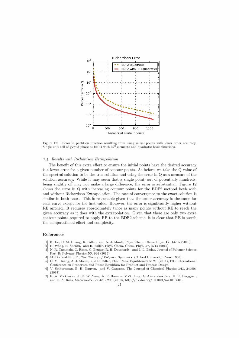
Figure 12: Error in partition function resulting from using initial points with lower order accuracy.Single unit cell of gyroid phase at f=0.4 with 323 elements and quadratic basis functions.
7.4. Results with Richardson Extrapolation
The benefit of this extra effort to ensure the initial points have the desired accuracyis a lower error for a given number of contour points. As before, we take the Q value ofthe spectral solution to be the true solution and using the error in Q as a measure of thesolution accuracy. While it may seem that a single point, out of potentially hundreds,being slightly off may not make a large difference, the error is substantial. Figure 12shows the error in Q with increasing contour points for the BDF2 method both withand without Richardson Extrapolation. The rate of convergence to the exact solution issimilar in both cases. This is reasonable given that the order accuracy is the same foreach curve except for the first value. However, the error is significantly higher withoutRE applied. It requires approximately twice as many points without RE to reach thegiven accuracy as it does with the extrapolation. Given that there are only two extracontour points required to apply RE to the BDF2 scheme, it is clear that RE is worththe computational effort and complexity.
References
[1] K. Do, D. M. Huang, R. Faller, and A. J. Moule, Phys. Chem. Chem. Phys. 12, 14735 (2010).[2] H. Wang, B. Shentu, and R. Faller, Phys. Chem. Chem. Phys. 17, 4714 (2015).[3] N. R. Tummala, C. Risko, C. Bruner, R. H. Dauskardt, and J.-L. Brdas, Journal of Polymer Science
Part B: Polymer Physics 53, 934 (2015).[4] M. Doi and E. S.F., The Theory of Polymer Dynamics. (Oxford University Press, 1986).[5] D. M. Huang, A. J. Moule, and R. Faller, Fluid Phase Equilibria 302, 21 (2011), 12th International
Conference on Properties and Phase Equilibria for Product and Process Design.[6] V. Sethuraman, B. H. Nguyen, and V. Ganesan, The Journal of Chemical Physics 141, 244904
(2014).[7] R. A. Mickiewicz, J. K. W. Yang, A. F. Hannon, Y.-S. Jung, A. Alexander-Katz, K. K. Berggren,
and C. A. Ross, Macromolecules 43, 8290 (2010), http://dx.doi.org/10.1021/ma101360f .
21

[8] S. T. Milner, T. A. Witten, and M. E. Cates, Macromolecules 21, 2610 (1988),http://dx.doi.org/10.1021/ma00186a051 .
[9] M. Muller, Phys. Rev. E 65, 030802 (2002).[10] A. D. Price, S.-M. Hur, G. H. Fredrickson, A. L. Frischknecht, and D. L. Huber, Macromolecules
45, 510 (2012), http://dx.doi.org/10.1021/ma202542u .[11] S.-M. Hur, A. L. Frischknecht, D. L. Huber, and G. H. Fredrickson, Soft Matter 7, 8776 (2011).[12] X. Zhu, L. Wang, J. Lin, and L. Zhang, ACS Nano 4, 4979 (2010), pMID: 20722410,
http://dx.doi.org/10.1021/nn101121n .[13] R. B. Thompson, V. V. Ginzburg, M. W. Matsen, and A. C. Balazs, Science 292, 2469 (2001),
http://www.sciencemag.org/content/292/5526/2469.full.pdf .[14] N. E. Jackson, K. L. Kohlstedt, B. M. Savoie, M. O. de la Cruz, G. C. Schatz, L. X. Chen,
and M. A. Ratner, Journal of the American Chemical Society 137, 6254 (2015), pMID: 25920989,http://dx.doi.org/10.1021/jacs.5b00493 .
[15] T. Geisinger, M. Mller, and K. Binder, The Journal of Chemical Physics 111, 5241 (1999).[16] C. E. Sing, J. W. Zwanikken, and M. Olvera de la Cruz, Nat Mater 13, 694 (2014).[17] C. E. Sing, J. W. Zwanikken, and M. O. de la Cruz, Phys. Rev. Lett. 111, 168303 (2013).[18] N. Laachi, T. Iwama, K. T. Delaney, D. Shykind, C. J. Weinheimer, and G. H. Fredrickson, Journal
of Polymer Science Part B: Polymer Physics 53, 317 (2015).[19] M. W. Matsen and R. B. Thompson, The Journal of Chemical Physics 111, 7139 (1999).[20] M. W. Matsen, The Journal of Chemical Physics 113, 5539 (2000).[21] Z. Guo, G. Zhang, F. Qiu, H. Zhang, Y. Yang, and A.-C. Shi, Phys. Rev. Lett. 101, 028301 (2008).[22] Y. Xu, W. Li, F. Qiu, and Z. Lin, Nanoscale 6, 6844 (2014).[23] M. W. Matsen, Macromolecules 45, 2161 (2012), http://dx.doi.org/10.1021/ma202782s .[24] J. R. Brown, S. W. Sides, and L. M. Hall, ACS Macro Letters 2, 1105 (2013),
http://dx.doi.org/10.1021/mz400546h .[25] G. Fredrickson, The Equilibrium Theory of Inhomogeneous Polymers, International Series of Mono-
graphs on Physics (OUP Oxford, 2005).[26] K. . Rasmussen and G. Kalosakas, Journal of Polymer Science Part B: Polymer Physics 40, 1777
(2002).[27] . Eric W. Cochran, *, . Carlos J. Garcia-Cervera, , and . Glenn H. Fredrickson*, , Macromolecules
39, 2449 (2006), http://dx.doi.org/10.1021/ma0527707 .[28] A. Ranjan, J. Qin, , and D. C. Morse*, Macromolecules 41, 942 (2008),
http://dx.doi.org/10.1021/ma0714316 .[29] G. Tzeremes, K. O. Rasmussen, T. Lookman, and A. Saxena, Phys. Rev. E 65, 041806 (2002).[30] P. Stasiak and M. W. Matsen, The European Physical Journal E 34, 1 (2011).[31] D. J. Audus, K. T. Delaney, H. D. Ceniceros, and G. H. Fredrickson, Macromolecules 46, 8383
(2013), http://dx.doi.org/10.1021/ma401804j .[32] L. F. Richardson, Philosophical Transactions of the Royal Society of London A: Mathematical,
Physical and Engineering Sciences 210, 307 (1911).[33] S. Balay, S. Abhyankar, M. F. Adams, J. Brown, P. Brune, K. Buschelman, L. Dalcin, V. Eijkhout,
W. D. Gropp, D. Kaushik, M. G. Knepley, L. C. McInnes, K. Rupp, B. F. Smith, S. Zampini, andH. Zhang, “PETSc Web page,” http://www.mcs.anl.gov/petsc (2015).
[34] S. Balay, S. Abhyankar, M. F. Adams, J. Brown, P. Brune, K. Buschelman, L. Dalcin, V. Eijkhout,W. D. Gropp, D. Kaushik, M. G. Knepley, L. C. McInnes, K. Rupp, B. F. Smith, S. Zampini,and H. Zhang, “PETSc users manual,” Tech. Rep. ANL-95/11 - Revision 3.6 (Argonne NationalLaboratory, 2015).
[35] S. Balay, W. D. Gropp, L. C. McInnes, and B. F. Smith, in Modern Software Tools in ScientificComputing, edited by E. Arge, A. M. Bruaset, and H. P. Langtangen (Birkhauser Press, 1997) pp.163–202.
[36] G. Karypis and K. Schloegel, “ParMETIS Web page,” http://glaros.dtc.umn.edu/gkhome/metis/
parmetis/overview (2013).[37] B. Bode, M. Butler, T. Dunning, W. Gropp, T. Hoefler, W. mei Hwu, and W. Kramer, The Blue
Waters Super-System for Super-Science, edited by J. Vetter, Contemporary HPC Architectures(Chapman and Hall/CRC, 2012) pp. 339–366.
22