Technical Report Documentation Page 1. Report No. 2. 3. Recipients Accession No. CTS 13-28 4. Title and Subtitle 5. Report Date A Fast, Auction-Based Algorithm for Paratransit Vehicle Assignment

September 2013 6.

7. Author(s) 8. Performing Organization Report No. John Gunnar Carlsson and Jason Houle

9. Performing Organization Name and Address 10. Project/Task/Work Unit No. Department of Industrial and Systems Engineering University of Minnesota 111 Church Street, SE Minneapolis, MN 55455

CTS Project #2011112 11. Contract (C) or Grant (G) No.

12. Sponsoring Organization Name and Address 13. Type of Report and Period Covered Center for Transportation Studies University of Minnesota 200 Transportation and Safety Building 511 Washington Ave. SE Minneapolis, MN 55455

Final Report 14. Sponsoring Agency Code

15. Supplementary Notes http://www.cts.umn.edu/Publications/ResearchReports/ 16. Abstract (Limit: 250 words)

A problem based on the actual passenger transportation operations of two community disability service organizations in St. Paul is presented. The problem is to minimize the number of routes needed to serve all the passengers subject to spatial and temporal constraints on the routing of vehicles. Additional problem characteristics include heterogeneous vehicle and passenger classes, multiple destinations, separate "runs" defined by service time windows, and rules governing the embarkment as well as maximum travel times. Here we develop a method able to generate a good problem solution within a reasonable amount of time to guide these companies' operations.

Early attempts at problem solution reveal facets of its structure and illuminate an inherent trade-off between vehicle capacity and uninhibited vehicle operating time. To address this, the method proposed uses high-capacity vehicles to serve routes in both runs while allotting easily served passengers to these vehicles to relieve temporal constraints. This heuristic carries the additional advantage of partitioning the rest of the solution into two single-run problems, and the decrementing adaptive memory program (DAMP) is devised as a way of discovering solution components and promoting those more effective at producing good solutions to be used in future attempts. When applied to a data set provided by the organizations, the algorithm improved the current benchmark solution, generated by hand, by over 12% in reasonable operating time, serving 574 passengers with 64 routes in 53 vehicles. Its absolute measure of quality, in light of lower bounds that were constructed, is also considered good.

17. Document Analysis/Descriptors 18. Availability Statement Community transportation, Physically handicapped persons, Paratransit services, Dispatching

No restrictions. Document available from: National Technical Information Services, Alexandria, VA 22312

19. Security Class (this report) 20. Security Class (this page) 21. No. of Pages 22. Price Unclassified Unclassified 64

A Fast, Auction-Based Algorithm for Paratransit Vehicle Assignment

Final Report

Prepared by:

John Gunnar Carlsson Jason Houle

Department of Industrial and Systems Engineering

University of Minnesota

September 2013

Published by:

Center for Transportation Studies University of Minnesota

200 Transportation and Safety Building 511 Washington Ave. S.E.

Minneapolis, Minnesota 55455

This report represents the results of research conducted by the authors and does not necessarily represent the views or policies of the University of Minnesota. The authors and the University of Minnesota do not endorse products or manufacturers. Any trade or manufacturers’ names that may appear herein do so solely because they are considered essential to this report.

Acknowledgments

The authors gratefully acknowledge the Center for Transportation Studies at the University of Minnesota for providing financial assistance to support the research in this document. Jason Houle also thanks Bill Cooper and the entire Department of Industrial and Systems Engineering at the University of Minnesota for their academic support.

Table of Contents

Chapter 1. Introduction ............................................................................................................. 1

1. Problem Statement ................................................................................................................. 1

2. Subject Overview ................................................................................................................... 1

3. Research Objective ................................................................................................................ 3

4. Organization of Report .......................................................................................................... 4

Chapter 2. Literature Review ................................................................................................... 5

1. The Dial-a-Ride Problem (DARP) ......................................................................................... 5

2. The Vehicle Routing Problem (VRP) and its Variants .......................................................... 6

3. Adaptive Memory Programming (AMP) ............................................................................... 7

Chapter 3. Routing Problem Model ....................................................................................... 11

1. A Mixed-Integer Nonlinear Program (MINLP) ................................................................... 11

2. Model Framework and Notation .......................................................................................... 13

2.1. Model Framework ......................................................................................................... 14

2.2. Model Notation ............................................................................................................. 14

Chapter 4. Solution Approach ................................................................................................ 16

1. General Assumptions ........................................................................................................... 16

2. Preliminary Studies .............................................................................................................. 16

2.1. Solving Runs Separately and Combining ...................................................................... 17

2.2. Remove and Reinsert ..................................................................................................... 18

2.3. Complete Partitioning by Run ...................................................................................... 19

2.4. “Filling in” Routes ....................................................................................................... 19

3. Problem Features and Insights ............................................................................................. 20

3.1. Centrally-Located Destinations .................................................................................... 20

3.2. Passenger Distribution ................................................................................................. 20

3.3. Vehicle Constraints ....................................................................................................... 20

4. Heuristics ............................................................................................................................. 21

4.1. Vehicle Assigned to Routes, Configured by Run ........................................................... 21

4.2. Radial “Deadheading” Pattern .................................................................................... 21

4.3. Weighting Passengers and Clusters .............................................................................. 23

4.4. Vehicle Tiering .............................................................................................................. 23

5. Subroutines .......................................................................................................................... 24

5.1. Evaluate Common Route Features ............................................................................... 24

5.2. Validity Checks ............................................................................................................. 25

5.3. Verify Vehicle ................................................................................................................ 27

6. Overview of Complete Algorithm ....................................................................................... 27

6.1. Estimate Objective Function Value for both Runs ........................................................ 29

6.2. Serve all Handicapped A Run Passengers .................................................................... 30

6.3. Serve Nonambulatory B Run Passengers with those Vehicles ...................................... 31

6.4. Exhaustively fill in Two-Run Routes with Ambulatory Passengers .............................. 35

6.5. Solve Remaining A and B Runs Separately with DAMP ............................................... 37

6.6. Summary ....................................................................................................................... 41

Chapter 5. Case Study ............................................................................................................. 43

1. Results from Actual Problem ............................................................................................... 43

2. Discussion ............................................................................................................................ 46

Chapter 6. Conclusion ............................................................................................................. 47

1. General Conclusions ............................................................................................................ 47

2. Directions for Future Research ............................................................................................ 48

2.1. Improving Elements of this algorithm........................................................................... 48

2.2. Expanding on Ideas Introduced .................................................................................... 49

References ................................................................................................................................. 51

Appendix A MATLAB Code

List of Figures

Figure 4.1: Best-known solution (in 1995) to problem of Christofides et al. [18] with 199 customers. Figure adapted from [7]. Paths to and from the depot are not drawn for clarity. ....... 22

Figure 5.1: The best A run routes obtained. Passengers are represented as black dots. Routes that share vehicles with B run routes are red, dotted lines; the other routes are black lines. Destinations are large, red squares. ............................................................................................... 44

Figure 5.2: The best B run routes obtained. Passengers are represented as black dots. Routes that share vehicles with A run routes are red, dotted lines; the other routes are black lines. Destinations are large, red squares. ............................................................................................... 45

List of Tables

Table 5.1: Results from case study solution. A stands for ambulatory, NA for nonambulatory, and WC for wheelchair. ................................................................................................................ 43

Executive Summary

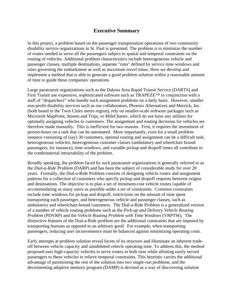
In this project, a problem based on the passenger transportation operations of two community disability service organizations in St. Paul is presented. The problem is to minimize the number of routes needed to serve all the passengers subject to spatial and temporal constraints on the routing of vehicles. Additional problem characteristics include heterogeneous vehicle and passenger classes, multiple destinations, separate "runs" defined by service time windows and rules governing the embarkment as well as maximum travel times. Here we develop and implement a method that is able to generate a good problem solution within a reasonable amount of time to guide these companies' operations.

Large paratransit organizations such as the Dakota Area Rapid Transit Service (DARTS) and First Transit use expensive, sophisticated software such as TRAPEZE™ in conjunction with a staff of “dispatchers” who handle such assignment problems on a daily basis. However, smaller non-profit disability services such as our collaborators, Phoenix Alternatives and Merrick, Inc. (both based in the Twin Cities metro region), rely on smaller-scale software packages such as Microsoft MapPoint, Streets and Trips, or MileCharter, which do not have any utilities for optimally assigning vehicles to customers. The assignment and routing decisions for vehicles are therefore made manually. This is inefficient for two reasons. First, it requires the investment of person-hours on a task that can be automated. More importantly, even for a small problem instance consisting of (say) 30 customers, optimal routing and assignment can be a difficult task; heterogeneous vehicles, heterogeneous customer classes (ambulatory and wheelchair bound passengers, for instance), time windows, and variable pickup and dropoff times all contribute to the combinatorial intractability of the problem.

Broadly speaking, the problem faced by such paratransit organizations is generally referred to as the Dial-a-Ride Problem (DARP) and has been the subject of considerable study for over 20 years. Formally, the Dial-a-Ride Problem consists of designing vehicle routes and assignment patterns for a collection of customers who specify pickup and dropoff requests between origins and destinations. The objective is to plan a set of minimum-cost vehicle routes capable of accommodating as many users as possible under a set of constraints. Common constraints include time windows for pickup and dropoff, restrictions on the amount of time spent transporting each passenger, and heterogeneous vehicle and passenger classes, such as ambulatory and wheelchair-bound customers. The Dial-a-Ride Problem is a generalized version of a number of vehicle routing problems such as the Pick-up and Delivery Vehicle Routing Problem (PDVRP) and the Vehicle Routing Problem with Time Windows (VRPTW). The distinctive features of the Dial-a-Ride problem are the additional constraints that are imposed by transporting humans as opposed to an arbitrary good. For example, when transporting passengers, reducing user inconvenience must be balanced against minimizing operating costs.

Early attempts at problem solution reveal facets of its structure and illuminate an inherent trade-off between vehicle capacity and uninhibited vehicle operating time. To address this, the method proposed uses high-capacity vehicles to serve routes in both runs while allotting easily served passengers to these vehicles to relieve temporal constraints. This heuristic carries the additional advantage of partitioning the rest of the solution into two single-run problems, and the decrementing adaptive memory program (DAMP) is devised as a way of discovering solution

components and promoting those more effective at producing good solutions to be used in future attempts. When applied to a data set provided by the organizations, the algorithm improved the current benchmark solution, generated by hand, by over 12% in reasonable operating time, serving 574 passengers with 64 routes in 53 vehicles. Its absolute measure of quality, in light of lower bounds that were constructed, is also considered good.

1

Chapter 1. Introduction

1. Problem Statement

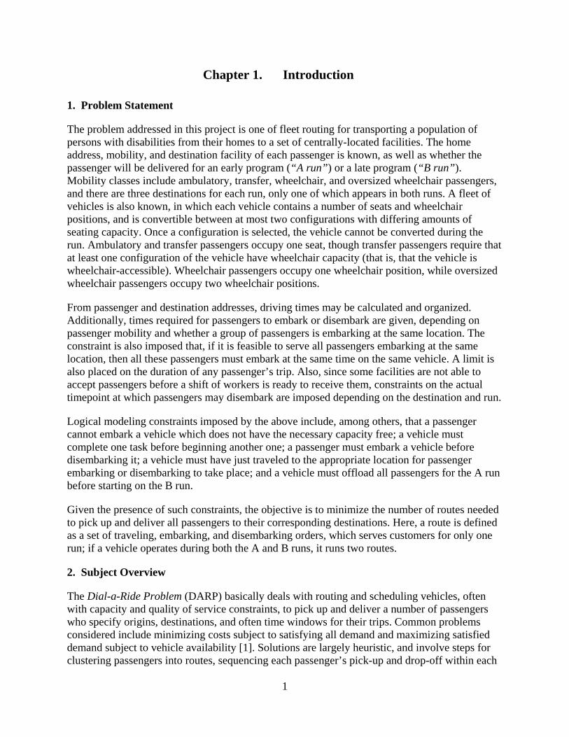
The problem addressed in this project is one of fleet routing for transporting a population of persons with disabilities from their homes to a set of centrally-located facilities. The home address, mobility, and destination facility of each passenger is known, as well as whether the passenger will be delivered for an early program (“A run”) or a late program (“B run”). Mobility classes include ambulatory, transfer, wheelchair, and oversized wheelchair passengers, and there are three destinations for each run, only one of which appears in both runs. A fleet of vehicles is also known, in which each vehicle contains a number of seats and wheelchair positions, and is convertible between at most two configurations with differing amounts of seating capacity. Once a configuration is selected, the vehicle cannot be converted during the run. Ambulatory and transfer passengers occupy one seat, though transfer passengers require that at least one configuration of the vehicle have wheelchair capacity (that is, that the vehicle is wheelchair-accessible). Wheelchair passengers occupy one wheelchair position, while oversized wheelchair passengers occupy two wheelchair positions.

From passenger and destination addresses, driving times may be calculated and organized. Additionally, times required for passengers to embark or disembark are given, depending on passenger mobility and whether a group of passengers is embarking at the same location. The constraint is also imposed that, if it is feasible to serve all passengers embarking at the same location, then all these passengers must embark at the same time on the same vehicle. A limit is also placed on the duration of any passenger’s trip. Also, since some facilities are not able to accept passengers before a shift of workers is ready to receive them, constraints on the actual timepoint at which passengers may disembark are imposed depending on the destination and run.

Logical modeling constraints imposed by the above include, among others, that a passenger cannot embark a vehicle which does not have the necessary capacity free; a vehicle must complete one task before beginning another one; a passenger must embark a vehicle before disembarking it; a vehicle must have just traveled to the appropriate location for passenger embarking or disembarking to take place; and a vehicle must offload all passengers for the A run before starting on the B run.

Given the presence of such constraints, the objective is to minimize the number of routes needed to pick up and deliver all passengers to their corresponding destinations. Here, a route is defined as a set of traveling, embarking, and disembarking orders, which serves customers for only one run; if a vehicle operates during both the A and B runs, it runs two routes.

2. Subject Overview

The Dial-a-Ride Problem (DARP) basically deals with routing and scheduling vehicles, often with capacity and quality of service constraints, to pick up and deliver a number of passengers who specify origins, destinations, and often time windows for their trips. Common problems considered include minimizing costs subject to satisfying all demand and maximizing satisfied demand subject to vehicle availability [1]. Solutions are largely heuristic, and involve steps for clustering passengers into routes, sequencing each passenger’s pick-up and drop-off within each

2

route, and scheduling the vehicle to serve the route. Wong and Bell [2] constructed a parallel insertion algorithm for solving the DARP with multi-dimensional capacity constraints, representing ambulatory and wheelchair passengers, and introduced a system to rank customers for insertion to routes by a weighted sum of factors, including mobility, earliest pick-up time, loading and unloading times at origin and destination, and decentralization. Despite this and related work, no set approach to the problem posed here is documented in the literature, either exactly like the one framed here or very close to it.

The vehicle routing problem (VRP) and its variants are special cases of the DARP, but precede the problem in the literature; thus, these problems have not only been handled for a longer time, but also more intensively, since they are much more approachable than the full DARP. Solomon [3] successfully constructed and analyzed a sequential, route-building insertion heuristic, which finds and records the optimal feasible position (if any) for inserting every unserved customer, then compares the extra distance and extra time that (individual) insertion of each customer at his respective optimal feasible position would require, selecting and adding the customer that minimizes a weighted sum of the two. Baldacci et al. [4] discuss reformulating VRPs as set partitioning problems, where the set in question is the set of all feasible routes for the problem; these routes are weighted as they would be in the original problem formulation (usually by fixed vehicle costs and/or variable link travel costs) and selected so as to minimize the sum of their weights subject to the constraint that each customer be served. Construction of lower bounds is also discussed, and it is the observation of minimizing cost by considering radial links that contributes most to the problem at hand. While a greater diversity of VRP variants have been studied than DARP variants, the basic problem is farther removed from the problem at hand; however, examination of the VRP is not complete without discussing a modern method developed recently to address it.

Glover [5] proposed a strategy for imposing surrogate constraints in solving integer programs heuristically, and directed the development of adaptive memory programming (AMP). After decades of work implementing these strategies in various forms, Taillard et al. [6] outline a generalized AMP as:

1. Initialize the memory. 2. While a stopping criterion is not met do:

(a) Generate a new provisional solution using data stored in the memory. (b) Improve by a local search; let be the improved solution. (c) Update the memory using the pieces of knowledge brought by .

This generalized form has been used to store and improve routes [7] or parts of routes [8, 9] in the memory bank, which are then combined to form new solutions and improved by local search improvement methods. The approach has been used to generate best-in-class solution methods for VRP variants including the heterogeneous vehicle VRP [10, 11] and the multi-depot VRP with inter-depot routes [12], though none of the methods discussed approach a problem general enough for direct or near-direct application without significant adjustment. AMP is a useful technique for solving problems such as the one at hand, but while a great deal stands to be garnered from the work on the DARP and VRP, novel methods need to be developed for a cohesive and efficient solution approach.

3

3. Research Objective

The problem was presented by two community disability service companies in St. Paul, Minnesota, looking to consolidate door-to-door transportation offered to their clients. The problem statement was constructed directly from the real-life structure of this problem, and the objective was explicitly specified by the companies involved, which considered the single objective of minimizing the number of routes needed (and thereby the cost of labor for drivers) to greatly outweigh considerations of number of vehicles used, trip duration or miles driven. Values for parameters (such as embarking times) resulted from discussions with the companies, and can be altered for use in the algorithm in the event that the companies do empirical studies to find suitable values for them. The motivation for solving this problem stems directly from the presence of this problem in the companies’ transportation planning operations, and its practical use for such remains an intrinsic part of the evaluation of its suitability.

The problem statement may be posed in the form of a mixed integer-linear program. However, the size of the problem makes its solution by means of globally optimal branch-and-bound methods highly impractical. Furthermore, an optimal solution is not necessary, and a good solution that is found quickly is more valuable than a slightly better one that requires a long time and great computing power to discover.

The objective of this research, then, is to develop an heuristic algorithm to produce a good solution; that is, a small number of feasible routes, within an amount of time acceptable to the companies for use in their operations. The companies undergo constant changes in their customer lists, though with a greater influx in the late spring, when new clients have graduated out of state-provided school disability services; as such, routes change no more than a few times per year. Ideally, the algorithm should provide its solution, operating on a standard desktop computer, in no more than a 15-hour overnight run.

Additionally, the objective of this work has been to address specifically the question at hand in its current form, rather than a generalized, abstract set of problems. A future goal that will benefit from this work is to provide these companies with a standalone computer application that implements the algorithm on a set of data. To this end, many specific features of the passenger dataset provided for this work are not examined or exploited. However, many features of the problem (such as the presence of three facilities in one run, all located a few minutes apart from each other) are (quite reasonably) assumed constant regardless of the passenger data. These features are considered and, where appropriate, exploited by implementing heuristics in order to improve the quality of the solution obtained. At the same time, this exploitation reduces the general applicability of the algorithm. For instance, if one company were to open another facility near the first three, some parts of the heuristic would need to be adjusted and reassessed; if the company were far away from the first three, additional steps would need to be taken to relax some of the algorithm’s assumptions and objectives. Throughout this document, an attempt is made to highlight the areas where the structure of the specific problem has been exploited, both as an explanation of the development of the algorithm in its current form, and to distinguish heuristics that may have general applicability from those developed within the context of this problem specifically.

4

4. Organization of Report

The remainder of this report is organized as follows:

• Chapter 2 provides a review of work previously done in related fields. • In Chapter 3, the problem is presented as a mixed integer linear program, with a

discussion of the constraints as they are manifested in the specific problem handled here. The model framework is also discussed.

• Chapter 4 contains the approach used in generating a solution. The chapter includes discussion of preliminary studies and the insights gained from these, as well as a detailed exposition of the heuristics that comprise the complete solution algorithm.

• Chapter 5 documents the results of the problem’s motivating case study. Methods for finding lower bounds are also discussed in order to illuminate the quality of the solution found.

• Chapter 6 summarizes the work with conclusions that may be drawn, and discusses future directions for research.

5

Chapter 2. Literature Review

A number of problems related to the one presented here have been handled in the literature. Intellectual predecessors are highlighted with an aim at noting the advances made in the field and the value of those to this problem, as well as points where this applied problem deviates from those cases already considered.

1. The Dial-a-Ride Problem (DARP)

The Dial-a-Ride Problem (DARP) basically deals with routing and scheduling vehicles, often with capacity and/or passenger type constraints, to pick up and deliver a number of passengers who specify origins, destinations, and often time windows for their trips. The idea of quality of service to passengers, either as an objective or a constraint, is a key difference in the DARP with respect to many other fleet routing problems. While most work has been done on the static problem, where all requests are known in advance of routing and scheduling, recent work has started to focus more on the dynamic DARP, where passengers can call and make a request while vehicles are running, requiring a dynamic adjustment of partially completed vehicle routes. Other variants include those with multiple depots and heterogeneous vehicle and passenger classes (all of which are features of the problem at hand), and common problems considered include minimizing costs subject to satisfying all demand and maximizing satisfied demand subject to vehicle availability [1].

The DARP is usually solved in three steps: clustering passengers into routes, sequencing each passenger’s pick-up and drop-off within each route, and scheduling the vehicle to serve the route. Cordeau [13] has published a review detailing both the DARP’s formulation and the approaches that have been taken to solve it. The multiple-vehicle case was not handled until Jaw et al.’s 1986 paper [14], though this and following work benefitted greatly from the single-vehicle work accomplished in the first half of the decade. For nearly two decades, these methods improved upon the procedures used to carry out the three steps mentioned, and grappled with the associated trade-offs. In 2003, Cordeau and Laporte [15] implemented a tabu search heuristic, which incorporated removal and reinsertion of passenger trips on a global scale and allowed intermediate infeasible solutions.

Wong and Bell [2] constructed a parallel insertion algorithm for solving the DARP with multi-dimensional capacity constraints, a variant that has received little explicit coverage in the literature. The model and approach follow Jaw et al. [14] but with a heterogeneous fleet of vehicles with two types of capacity: one each for ambulatory and wheelchair passengers. Vehicle capacities are assumed non-substitutable in this work, and only a simple case of two vehicle classes and two passenger classes is examined for computational studies. The parallel insertion heuristic comprises three sequential steps: ranking trips, parallel insertion of trips into routes, and an optional local search procedure, which seeks to improve the solution by examining neighboring solutions (e.g., by swapping a pair of passengers between routes) and moving to more optimal solutions. The first is a reponse to importance of sequencing passenger trips well to the effectiveness of insertion heuristics. To this end, Wong and Bell rank customers by a weighted sum of factors, including mobility, earliest pick-up time, loading and unloading times at origin and destination, and decentralization, such that the customers most inconvenient to

6

serve are ranked higher. The insertion heuristic operates by moving down this list and attempting to insert trips into feasible locations in routes, where feasibility depends upon satisfaction of time window, trip duration, capacity, and other relevant constraints (such as precedence). If one or more feasible locations are found, the trip is inserted in the one which increases the objective function least; otherwise, a taxi is used or some other penalty is charged for turning down the passenger. Finally, some of the computational studies included a "trip insertion" technique for local search, in which a trip is removed from its current route and position and inserted into a best feasible route and location within the present set. This improvement search is carried out for each trip until no improvements may be made, implying a local optimum. Using a randomly generated set of problems, this algorithm compared favorably with the classic parallel insertion algorithm of Solomon [3].

The most recent advances in the DARP and its variants have included work on the dynamic case, as well as formulation and rigorous analytical work aimed at finding algorithmic solutions. The branch-and-cut algorithm of Cordeau [16] is an early example of this latter set, and includes the basic problem formulation that is modified to describe this problem.

Despite the work in this field, there appears to be no set approach to problems either exactly like the one framed here or very close to it. For one, the objective of the problem at hand, minimizing the number of routes used to satisfy the demand of all passengers, differs greatly from that of the traditional DARP, which is to minimize the sum of the weights of the links chosen, subject to the same constraint. Additionally, aside from Bell and Wong [2], little work has been done on multidimensional vehicle capacities, and even that work did not consider substitutable capacity types. Other unique features of the problem, such as multiple depots and the two-run structure, provoke investigation of related problems to see if these facets have been handled somehwere in the literature.

2. The Vehicle Routing Problem (VRP) and its Variants

The vehicle routing problem (VRP), VRP with time windows (VRPTW), and pick-up and delivery VRP (PDVRP) are all special cases of the DARP, but precede the problem in the literature; thus, these problems have not only been handled for a longer time, but also more intensively, since they are much more approachable than the full DARP. The first two cases are only delivery problems, where each customer has a demand and a vehicle serving a route must have sufficient capacity to fill the demands of all customers on that route. In the VRPTW, some bounds exist on the time at which this must be accomplished. Of these three, only in the PDVRP is both an origin and destination associated with each customer.

Solomon [3] constructed and analyzed some of the earliest route-building heuristics for the VRPTW, taking into account temporal as well as spatial considerations. Of these, a sequential, route-building insertion heuristic was found to perform best on a range of randomly generated data sets. This heuristic finds and records the optimal feasible position (if any) for inserting every unserved customer, then compares the extra distance and extra time that (individual) insertion of each customer at his respective optimal feasible position would require, selecting and adding the customer that minimizes a weighted sum of the two. The heuristic borrows a principle from the “savings algorithm” also discussed, and the parameters for the weighted sum must be tuned;

7

nonetheless, this heuristic predates and corroborates the long-standing methods used in the seminal multi-vehicle DARP paper by Jaw et al. [14].

Baldacci et al. [4] review work done in another variant, the heterogeneous fleet VRP (HVRP), in which various constraints exist on a fleet of vehicles that are heterogeneous (though still one-dimensional) with respect to capacity. The closest variant to the case at hand is the site-dependent VRP (SDVRP), which includes limits on fleet size, no fixed vehicle costs, and compatibility requirements exist for a vehicle type to serve certain customers. The authors handle this set of variants extensively, discussing a range of heuristics and their respective performance measures for each variant. Notably, HVRPs can be formulated as set partitioning problems, where the set in question is the set of all feasible routes for the problem; these routes are weighted as they would be in the original problem formulation (usually by fixed vehicle costs and/or variable link travel costs) and selected so as to minimize the sum of their weights subject to the constraint that each customer be served. Construction of lower bounds is also discussed, and the notion of a route’s pivot, or the point in the route farthest from the depot, is introduced. Again considering an objective function including fixed vehicle and variable link travel costs, a lower bound is realizable as the sum, over every route in the optimal solution, of the fixed vehicle cost for the vehicle serving that route plus radial link travel cost from the depot to the pivot and back. While further analysis is carried out to construct a practical lower bound for this problem, it is the observation of minimizing cost by considering radial links that contributes most to the problem at hand.

While a greater diversity of VRP variants have been studied than DARP variants, the basic problem is farther removed from the problem at hand. Parts of these approaches to the HVRP and PDVRP may be cobbled together to produce a solution method, but many elements are still lacking from any approach, and the unique objective function and two-run structure will require additional innovation. However, examination of the VRP is not complete without discussing a modern method developed recently to address it, covered in the next section.

3. Adaptive Memory Programming (AMP)

It is clear from the complexity and size of the problem handled here that an heuristic approach is needed, since, despite the advances in methods used to find exact solutions, even the best branch-and-cut optimization algorithms cannot handle simpler cases than this one with as many as a hundred passengers in one run.[16] Since Glover’s lament in 1977 [5] that “algorithms are conceived in analytic purity in the high citadels of academic research, heuristics are midwifed by expediency in the dark corners of the practitioner’s lair,” heuristics have gained respect, especially in regards to handling complex problems such as the DARP and VRP. It was in that same paper that Glover laid the principles for the solution method used in this paper. He introduced notions of strongly determined variables and consistent variables (or those variables which tend to take on values in certain, small ranges in most or all good solutions), and a strategy for imposing “surrogate constraints” in order to focus the problem toward solutions incorporating these values [5]:

8

1. Select one or more variables with greatest relative consistencies and constrain these to their preferred values.

2. Determine new relative consistencies for the variables on the basis of the restriction of step 1.

3. Repeat the process until all variables have been constrained to specific values.

Rochat and Taillard [7] developed an algorithm to solve the VRP and VRPTW based on this procedure in 1995, which used a local search method developed by Taillard [17] to construct a set of solutions, then ranked the routes from each set of solutions according to the respective solution’s objective function value. From this list, routes were probabilistically selected for integration into a new solution, which was then further improved through local search. The resultant routes were then inserted into the list according to the solution’s objective function value; this process of combining, improving, and evaluating was iterated until a stopping criteria was satisfied. When applied to several sets of standard problems in the field, this method of “diversification and intensification” was shown to converge very quickly to solutions very close to the best known solution, and showed particular improvement in computation time over previous best algorithms in the case of large problems. Due to the structure of the algorithm, parallelization could readily be implemented for even greater speed gains. This was heralded as the seminal application to the VRP of a methodology later definitively christened by Taillard et al. [6] as adaptive memory programming (AMP).

Taillard et al. [6] discuss a range of generic heuristic methods, also known as metaheuristics, that have been applied to the VRP, including genetic algorithms, scatter search, tabu search, ant systems, and the heuristic of Rochat and Taillard [7]. Many hybrid methods of these also exist due to common features such as improving solutions based on a memory of previously discovered, good partial solutions. From these [6], a generalized AMP is outlined as:

1. Initialize the memory. 2. While a stopping criterion is not met do:

(a) Generate a new provisional solution using data stored in the memory. (b) Improve by a local search; let be the improved solution. (c) Update the memory using the pieces of knowledge brought by .

Each manfestation achieves these steps in different ways and depends upon the problem being handled, as well as heuristics or algorithms available for steps like 1 and 2(b).

Despite the definition of AMP coming from leaders in the VRP field, and the fact that VRP applications were discussed in some detail in the paper in which AMP was defined [6], Tarantilis [9] writes in 2005 that “only two pure AMP algorithms for solving the capacitated VRP have been presented to-date;” these are the BoneRoute algorithm, constructed by Tarantilis and Kiranoudis [8], and Rochat and Taillard’s [7] VRP AMP algorithm, upon which BoneRoute is meant to be an improvement. BoneRoute generates and stores “bones”, or parts of routes in solutions, then combining these by use of a construction heuristic to form new routes and, by extension, solutions, again using a local search method for the purpose of diversifying the memory pool. Tarantilis [9] followed this up a couple years later with the Solutions’ Elite PArts Search (SEPAS). “Elite parts,” like bones, are route components which are memorized and evaluated in the AMP. Also unlike Rochat and Taillard [7], who select routes for construction of

9

new solutions from the ranked memory list probabilistically, the elite parts selected by SEPAS to build new solutions are selected deterministically following two selection criteria. SEPAS differs from both previous heuristics in that the initial memory is generated systematically and not stochastically, engineering a greater diversification of available components from the beginning of the algorithm. Additionally, the improvement heuristic used by SEPAS is a sophisticated tabu search with a long-term memory feature to improve the search’s ability to diversify and intensify solution sets. The benefit of these adaptations was shown when SEPAS consistently found solutions very near to best solutions, and discovered several new best solutions for large benchmark problem sets. In addition to this, it shares the advantages (as with most AMPs generally) of easy application to related VRP variants as well as to parallelization techniques.

Departing from the standard VRP, Taillard [10] extended the seminal VRP AMP algorithm to a VRP with heterogeneous vehicle types, essentially solving a separate VRP for each vehicle class and then gathering good routes produced using each vehicle, weighting them by the cost of servicing them by their respective vehicles, and selecting which vehicles and routes to include in the final solution by solving a set partitioning program, formulated as a boolean linear program, in CPLEX. Gendreau et al. [11] combined the use of the “GENIUS” insertion and improvement algorithm with tabu search for a globally-focused AMP approach, and attacked a common set of problems as Taillard, with results that were generally comparable, though compared favorably in terms of computing time on larger problems due to Taillard’s solution of the boolean linear program.

Crevier et al. [12] also introduced an algorithm to solve the multi-depot VRP with inter-depot routes (MDVRPI), a problem in which multiple depots exist and vehicles can travel along routes between depots, using these as replenishment points, e.g. for making deliveries. Their metaheuristic includes a method for generation of a solution pool that combines results from decomposing the problem into each a mutli-depot VRP, several separate VRPs, and inter-depot subproblems, and their contributions include a detailed review of similar methods as well as the establishment of benchmark problems for comparison of MDVRPI heuristics.

The metaheuristic approach has clearly advanced the work done to find a heuristic solution to the VRP and its variants. Of course, just as in section 2, the problems discussed remain significantly removed from the complex problem handled here. As such, while the AMP framework will be used in the development of a comprehensive metaheuristic for solving the problem at hand, none of the methods discussed approach problem general enough for direct or near-direct application without significant adjustment. As will be discussed in section 2, the local search methods (and neighborhood framework that accompany them) that dominate AMP studies are difficult to apply to this problem in practice. Even with advanced methods such as SEPAS [9] available to solve the VRP, complex constraints inhibit its usefulness, and difficulties with trying to force such an approach into the two-run structure are discussed later in this work. Notably, although Crevier et al. [12] handle a problem in which vehicles may serve passengers after returning to a depot, providing an avenue for applying the AMP to the two-run structure, their problem includes neither pick-up and delivery aspects nor time windows, which are key constraints in the problem handled.

10

Moreover, it must be remembered that the objective functions of the VRP and the problem handled here are different, and advances made with diminishing marginal returns in solving the VRP may not be as useful for solving the problem presented here. While a great deal stands to be garnered from the work on the DARP and VRP, novel methods need to be developed for a cohesive and efficient solution approach.

11

Chapter 3. Routing Problem Model

In this chapter, the problem presented will be formally described as a mixed integer-linear program, based on its relationship to the DARP. This program will be related to the problem at hand, and then details of the heuristic modeling framework used will be discussed.

1. A Mixed-Integer Nonlinear Program (MINLP)

This formulation, including much of the notation, is derived from the one presented by Cordeau [16]. The main idea is to formulate our problem as a mixed-integer nonlinear program (MINLP), that is, a mathematical optimization problem in which some of the variables are required to be integers. In the following objective function and constraints, represents the number of passengers to be served, indexed by . Consider the directed network , where N represents the set of all nodes in the network (that is, all pickup nodes, dropoff nodes, and vehicle depots) and A represents the set of all arcs in the network (that is, all paths between a pair of nodes). Mathematically, we express this as , where are the pickup nodes and are corresponding dropoff nodes, such that passenger is picked up at node and dropped off at node . Nodes and are origin and destination depots. is the arc set and is complete (that is, there is an arc connecting every pair of nodes), and with each arc is associated a travel time .

Note that this is a generalization of the problem presented, since there are only 5 different destinations instead of . Also, each pick-up node may contain more than one passenger; this is handled by grouping them all into a common load due to the constraint (not expressed below) that passengers at a common residence should all embark together. If the passengers encompass such a load that they cannot fit on one vehicle, then they are separated into two or more groups, and the constraint is necessarily relaxed. This is done in preprocessing; from here, both individual passengers and groups of passengers will be referred to as “passenger.”

The set of vehicles is denoted by , and each vehicle has two configurations for capacity, where is the indicator variable that vehicle is configured to maximize the ambulatory capacity. Each vehicle also has two-entry vector capacities and , which include ambulatory capacity and wheelchair capacity and represent the ambulatory capacity-maximizing configuration and wheelchair capacity-maximizing configuration, respectively. With each node is associated a two-entry vector load that includes ambulatory capacity and wheelchair capacity, such that and . Associated with each node is a service time duration, . For pick-up nodes, this value is related to the passenger’s mobility and any grouping of individual passengers at the same node. For drop-off nodes, the problem at hand uses a set value. A time window is also associated with node , where and are the earliest and latest permissible times for service to begin at node . Also let denote the maximum travel time allowed for any passenger.

For each arc and each vehicle , let if vehicle travels from node to node . For each node and each vehicle , let be the time at which vehicle begins

service at node , and let the vector represent the load of vehicle after visiting node .

12

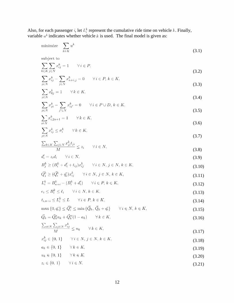
Also, for each passenger , let represent the cumulative ride time on vehicle . Finally, variable indicates whether vehicle is used. The final model is given as:

(3.1)

(3.2)

(3.3)

(3.4)

(3.5)

(3.6)

(3.7)

(3.8)

(3.9)

(3.10)

(3.11)

(3.12)

(3.13)

(3.14)

(3.15)

(3.16)

(3.17)

(3.18)

(3.19)

(3.20)

(3.21)

13

The objective function (3.1) minimizes the total number of vehicles used, which is determined in equation (3.17). Constraints (3.2) and (3.3) ensure that each request is served exactly once and that pick-up and drop-off for every passenger occurs with the same vehicle. Constraints (3.4), (3.5), (3.6) ensure that each route starts at the origin depot and ends at the destination depot; while these are not necessarily needed (or true) for the actual problem at hand, they help to frame and generalize the MINLP. Constraints (3.7), (3.8), and (3.9) are not in Cordeau’s [16] formulation; the first of these ensures that vehicles only serve passengers they are allowed to, while the second and third enforce a rule regarding common disembarkments. The inequalities in (3.10) and (3.11) enforce consistency in the variables accounting for time and load, while constraint (3.12) does the same for passenger duration, which value is bounded in constraint (3.14). Notably, the left inequality in this constraint also serves to enforce precedence, since it forces the variables to be nonnegative. Constraints (3.13) and (3.15) impose time windows and capacity constraints, respectively, while (3.16) forces the consistency of vehicle capacity depending on configuration.

Some of the problem constraints explained above bear no relevance on the problem’s solution since the objective function has changed from that of the classical DARP formulation; others are generalized, but only find actual applications in certain parts of the problem structure. For instance, constraints (3.4) and (3.6) force routes to start and end at depots; however, links from the depot to a beginning node, or from an ending node back to the depot, do not appear anywhere else in the formulation. These constraints are only implemented so that other constraints, such as (3.5), remain valid and simply stated.

The general constraint (3.7) is necessary for only one specific case in the problem. “Transfer” passengers are handicapped persons who can sit in ambulatory seats, but require a wheelchair lift for embarking a vehicle. Thus, while a 15-passenger van can accomodate such passengers in terms of capacity, it cannot actually serve these customers, requiring this additional constraint.

Constraints (3.8) and (3.9) allow enforcement of the modeling policy that all disembarkments take a set amount of time (in this case, 5 minutes) regardless of the number and mobility of passengers disembarking. The variables will only be zero (causing the corresponding to become zero) for drop-off nodes that are colocated with the previous drop-off node visited, and the effective drop-off duration will be the drop-off duration of only the first drop-off node visited. Note that sequential pick-up nodes may not be colocated due to the preprocessing efforts to group these passengers into single “passengers.”

The two-run structure is also entirely absent from this formulation, and must be imposed through use of time windows. A run passengers have no constraints on pick-up, but two facilities cannot accept passengers before 8am, imposing a constraint on drop-off. Also, all B run passengers are not to be dropped off later than 9:30am. Additional constraints may be imposed to ensure passengers are not dropped off at impractical times, e.g., hours before their sessions begin.

2. Model Framework and Notation

The above formulation is enormous and unwieldy. For the case study discussed here, the above formulation requires over 21.4 million variables and over 63.8 million constraints, including

14

integer and nonlinear constraints. As was discussed in the literature review, this problem is completely intractable for rigorous optimization, and an heuristic approach is needed.

2.1. Model Framework

The heuristic method used requires its own framework, which will be introduced here. This section will explain some of the structures and terms used in the heuristic approach.

Rather than consider each vehicle separately, vehicles are separated into “classes.” A vehicle class is one in which all members have identical and . These values, along with the number of vehicles of each class, are recorded in a “garage” memory structure, from which they may be read. This allows for more flexibility in assigning vehicles, since vehicles of a common class are completely interchangeable. The total count of vehicles in a class is all that is needed, rather than an identifier for each individual vehicle.

Due to the division of the A and B runs, the data set of each run is considered separately, and customers in each run are numbered from one – no vehicle is allowed to transport both A and B run passengers simultaneously. Necessary information to compose a route includes only the run the route is in, an ordered list of passengers that are picked up, an ordered list of destinations visited, the vehicle class, and the presence and identity of any route in the other run that shares the same vehicle. Given this, a set of times corresponding to travel and passenger embarkment and disembarkment may be generated, and the feasibility of the route with respect to all constraints may be evaluated.

For the sake of computational simplicity, the algorithm considers not routes but vehicles, storing routes that share a vehicle in separate parts of the same data structure. Given the constraints that routes using the same vehicle can impose on each other, verifying feasibility is more easily achieved. Additionally, to reduce the number of computations needed in subroutines, both the vehicle’s configuration and times associated with travel and embarkment/disembarkment are stored in the structure as well. The structures used separate travel into four parts: A run pick-up, A run drop-off, B run pick-up, and B run drop-off. These must take place sequentially without going backwards at any time.

The solution approach is to construct a pool of these route data structures. Various verification subroutines exist to ensure that all constraints that bound this pool of routes are met. The objective function is clearly calculated as the total number of routes. The approach taken to minimize this objective function is the subject of the next chapter.

2.2. Model Notation

For the rest of this paper, notation for these data structures will be as follows: the set of all A run passengers will be referred to as and indexed by while the set of all B run passengers will be referred to as and indexed by . The set of A run destinations will be , and the set of B run destinations will be . ( represents “midpoints,” while stands for “endpoints.”) Additional information required includes the travel time between any two nodes and , given by ; the destination of a passenger, given by or , depending on whether the passenger is in the A or B run; and the mobility of each passenger,

15

given by or , depending again on the passenger’s run. We set , where 1 represents ambulatory customers, a (1,0) load; 2 represents transfer customers, a (1,0) load; 3 represents wheelchair customers, a (0,1) load; and 4 represents oversized wheelchair customers, a (0,2) load. In the preceeding, the first entry is the load requiring ambulatory capacity, while the second entry is the load requiring wheelchair capacity.

A number of parameters also exist for the solution of the problem. These include and , which delineate the time window within which each run may operate, based on a standard of switching over around 8am. Thus, if both values are 90 minutes (as they are in the case study), the earliest that service on an A run route may start is 6:30am, while the latest that service on a B run route may start is 9:30am. Additional parameters include boarding times corresponding to different mobilities, as well as rules for adjusting these in the case of common embarkment. These will just be mentioned rather than spelled out explicitly, but the values used in the case study are 2.5 minutes for ambulatory passengers and 4 minutes for all other passengers. Multiple non-ambulatory passengers can board at a rate of 3 minutes per passenger, while multiple ambulatory passengers can board in 3 minutes flat. If ambulatory passengers board with nonambulatory passengers, their embarkment is counted as free.

During the problem solution, the set of served A run passengers will be denoted as and the set of served B run passengers as . The set of formed vehicles, , contains vehicles indexed by . The vehicle class may be denoted as and the vehicle’s configuration as , where a value of 1 represents the configuration maximizing ambulatory seats and a value of 2 represents the configuration maximizing wheelchair spaces. The vehicle also includes sequences , , , and , representing the nodes visited for A run pick-ups, A run drop-offs, B run pick-ups, and B run drop-offs, respectively. These may also be indexed as , , etc. Durations are also associated with all these parts; is the time needed to travel from node to the next visited node, and is the time needed to either drop off or pick up passengers at node , where can be any of , , , or . Note that can be the time between nodes in two different sequences, e.g., from the last node in to the first node in . Finally, and represent the actual timepoints that either the corresponding time travel or service are initiated.

16

Chapter 4. Solution Approach

1. General Assumptions

Several assumptions about the structure of the problem guided the algorithm’s development and use of heuristics. Highlighted here are the central location of destinations, the distribution of passengers between runs, the uniformity of passengers by class, and the use of software to determine point-to-point driving times used in evaluating route times.

The assumption of centrally-located destinations provides a conceptual paradigm for the construction of the routing algorithm. In the A run, the three facilities are no more than 10.4 minutes apart and as little as 6.6 minutes, while in the B run, the three facilities are no more than 12.6 minutes apart, and as little as 5.5 minutes. The proximity of the two companies’ facilities to each other was a motivating factor in posing this problem and supporting this work. Additionally, due to the geography and demographics of the region, the location of these facilities does not place them at any logical extreme with relation to the majority of passengers’ home locations, and a cursory examination of the data set is all that is needed to confirm that passengers are located with uniformly decreasing density in all directions away from the facilities. Such a structure is certainly not unique to the real-life case at hand, a fact that suggests that this algorithm might find use for other cases with minimal adaptation.

While the two-run structure is a novel consideration in this problem, there is also evidence of a distinction in passenger distribution between the runs. In the data set considered, 302 of the 352 A run passengers, or 85.8%, are ambulatory, while in the B run, only 110 of the 222 passengers, or 49.6%, are ambulatory. This is not a chance occurrence, but is a product of the different services and options provided by the companies to their clients; similar distributions persisted despite a number of changes to the customer list. The assumption going forward is that the A run contains more passengers, most of which are ambulatory, while the B run contains fewer passengers overall but more disabled passengers in total.

No distinction among passengers of common mobility is given, and thus all are assumed to have the same time needed for embarkment (except where multiple passengers embark at the same location). These embarkment times by passenger mobility are parameters in the algorithm and can be readily changed between runs, while rules regarding multiple embarkment as well as disembarkment are more complicated and hard-wired into the algorithm’s code - revising these requires a change of the basic script.

Finally, the distance matrix was calculated using Microsoft MapPoint® with the plug-in MileCharter. MileCharter generated the point-to-point travel times matrix, and its values for travel are assumed to be adequate approximations of actual driving time.

2. Preliminary Studies

A number of approaches were taken to different parts of the problem to explore the problem’s structure and avenues for exploitation. The most fruitful of these preliminary studies are discussed as a preamble to the final solution approach taken.

17

2.1. Solving Runs Separately and Combining

One of the first approaches taken was to separate the problem into runs, solving each run by first using a greedy algorithm to route a selection of vehicles through all the passengers, e.g., by assigning a vehicle to a random passenger and then adding the nearest unserved passenger to the route until no passenger could be found whose addition would not require a constraint to be broken, then utilizing a remove and reinsert algorithm to improve passenger assignment to vehicles, removing vehicles from the run solution when all passengers were removed and reinserted in other routes. Pairing of the A and B run routes produced in the solution of the individual runs was then attempted by use of a matching heuristic in order to increase utilization of high-capacity vehicles. Once vehicles were combined, as possible, another remove and reinsert algorithm was used to try to reduce the number of routes further, and then to finalize the solution obtained. This approach aligns well with the methods used by Tarantilis [9] in developing SEPAS, as well as the approach to the MDVRPI formulated by Crevier et al. [12], but never manifested itself fully as an instance of AMP due to a number of issues encountered.

Part of the problem with this approach was its aim; the objective function was not clearly defined at that time, and this approach was taken with the intention of reducing the number of vehicles used rather than the number of routes needed. However, the attempt to use this algorithm shed light on some of the difficulties inherent in the two-run approach. Specifically, many aspects of the algorithm ended up working against each other due to ignorance of elements of the problem structure. As the methods used to produce the initial greedy solutions and then to remove and reinsert passengers among them improved vehicle utilization and consequentially decreased slack in timing constraints and vehicle capacity constraints, the matching of A run routes to B run routes using the same vehicle became much more difficult. For one, since the amount of time available for a vehicle to operate in the B run is tied directly to its obligations in delivering A run passengers, solutions to either run imposed significant additional time constraints on routes in the other run using the same vehicle. Moreover, since vehicle configuration was determined during the individual run routing process as necessary, and since the distribution of passengers between runs usually required vehicles serving routes in the A run to be configured to serve more ambulatory passengers and vehicles serving routes in the B run to be configured to serve more handicapped passengers, matching of vehicles between the runs (with the constraint that any single vehicle be identically configured for both runs) became difficult and often impossible.

Additionally, one aspect of many advanced AMP methods is solution of a set-partitioning problem to select components for construction of a new solution. In the metaheuristic of Crevier et al. [12], one set partitioning step will often take one-half to two-thirds of the computation time, and sometimes more, for large problem sets. Gendreau et al. [11] also cites the choice to avoid such a step as an advantage for their algorithm, since “the set partitioning phase of Taillard’s [10] algorithm becomes rather time consuming when becomes large.” Due to the size and complexity of the problem at hand, and the desire stated in section 3 to produce a useful and, ideally, portable algorithm untethered from commercial software such as CPLEX for programming solutions, it was desirable to avoid employing set partitioning and the strategies that employ it.

Owing to the self-defeating nature of improving elements of this algorithm, as well as a redefinition of the problem’s objective, this approach was soon abandoned. Its legacy, however,

18

is important in that it provoked a shift of paradigm, from viewing the problem more from the scale of individual routes and vehicles to one requiring a comprehensive approach to forming routes, which accounts for the characteristics of both runs and the interplay between them. This shift was pervasive to the point of throwing out the old algorithm altogether, and inciting the reworking of the data structures used in addition to the general approach taken.

2.2. Remove and Reinsert

The local search approach of removing and reinserting passengers in sets of routes for improving solutions was used in the approach described in section 2.1, and was pursued in the next approach taken. However, as demonstrated in the previous approach, a number of obstacles exist to successfully implementing such a strategy given the structure of the problem at hand.

While this strategy could be implemented many ways, the obstacles eventually faced stemmed from the same characteristics of the problem. Removal of passengers proceeded either by random selection of passengers, or by removing the passenger whose removal produced the greatest decrease in the time required to service the route. Several passengers at a time were removed and then usually ordered by a weighting heuristic for reinsertion. Difficulties only arose in attempts to reinsert these passengers. Just as improved vehicle utilization and decreased slack in timing constraints and vehicle capacity constraints impeded the matching of A run routes to B run routes in the previous algorithm, it also hindered more and more the reinsertion of passengers. In the case studied, excess vehicle capacity was more abundant than excess route time in improved solutions, but reinsertion also required satisfaction of essentially spatial constraints – a passenger needed not only to fit into the respective vehicle to be inserted into a route, but also needed to be relatively close to the passengers already served in the route, to prevent exceeding time or passenger holding constraints.

A distinction must be drawn between this problem and previous problems, the solution methods to which successfully implemented advanced local search methods. Reinsertion requires slack to be present in routes, either in the form of time or of capacity, but as solutions are improved and vehicle utilization is increased, slack is removed, impeding further improvement. Such a strategy suffers from the paradox that, in terms of solution quality, slack is considered waste, whereas in terms of improvability, slack is valuable. Nonetheless, many studies implement this strategy with great success. The basic difference is the problem complexity: essentially, a strategy of reinsertion could yield little success in the complex environment of the problem currently studied, requiring so many constraints to be satisfied. Many of the most powerful approaches in both the VRP and the DARP [1, 7, 9, 12] assume that vehicles and passengers are identical, but both assumptions fall through here, creating a much more fractioned and complex problem with obstacles to simple tabu search methods that serve as improvement heuristics in these advanced algorithms. Moreover, since the objective is to reduce the number of routes needed to serve all passengers, the “neighborhood” framework in which local searches operate is disrupted; any number of passenger swaps can take place without effectively improving the problem objective function. The benefit of running such an improvement heuristic becomes less evident, and experience demonstrates that simple swaps resulting from, e.g., tabu search are ineffective for reducing the solution’s cost.

19

What was learned from this approach was that routes need to be set well the first time, as a group – simple improvement algorithms operating on a set of a priori routes must grapple with a range of obstacles owing to the problem structure, and are unlikely to yield a significantly improved solution cost.

2.3. Complete Partitioning by Run

Recognizing both that the number of routes was to be minimized regardless of the number of vehicles used, and that routes sharing a vehicle impose constraints on each other, a logical attempt was made to completely partition the problem by run, solving both from the same pool of vehicles. A modified “deadheading” procedure, following priniciples covered in section 4.2, was used, alternating between the A run and B run and assigning vehicles randomly to begin forming routes. This procedure bears resemblance to the lower-bounding ideas detailed in section 6.1, except that in this case, a feasible solution is sought and thus both runs simultaneously drew from the same vehicle pool to avoid overlap. No allowances were made for a vehicle to operate both runs.

The principles used to design this algorithm are valid for the problem and remain largely intact in the final method produced. Ideally, such a procedure would be used to solve the problem, though improvement of the routing algorithm used would certainly be welcome. The reason this was not further pursued is that it was quickly seen that insufficient wheelchair capacity existed in the vehicle pool to service all passengers in both runs without using some vehicles for both runs. Adding to this the considerations of the time and precedence constraints, this method was quickly understood to be incapable of producing a feasible solution. The results of this attempt framed the tradeoff of different strategies for vehicle use: using a vehicle in both runs doubles the capacity it offers to accommodate passengers, while using a vehicle in a single run allows a route to be formed without the imposition of time constraints due to the vehicle’s use in another run.

2.4. “Filling in” Routes

The term “filling in” routes will here be used to refer to a parallel insertion technique of pairing unserved passengers with feasible positions in existing routes. More specifically, while the practical aspects of this pairing is the same as is done in reinsertion steps, “filling in” will largely refer to a process beginning with a set of only sparsely populated routes and large numbers of unserved passengers, as opposed to reinsertion of a small number of unserved passengers into a set of routes with little slack. The strategy is used as a means of achieving a good set of routes to begin with, involving more involved computations and often a more global view of the problem than a simple, greedy algorithm. Its strong resemblance to reinsertion actually comes from its origination as an attempt at “reinsertion before removal.”

Filling in proceeds by “smallest additions,” not unlike Solomon’s insertion heuristics [3]: passengers are added to routes in a way that minimizes the additional time required to service the route. This can be accomplished by a completely exhaustive search, finding the passenger, route, and position in the route that is feasible and adds the smallest time to that individual route considered among all permutations. A much quicker strategy is to rank passengers (usually by spatial position, disability, and requirements for common embarkment with other passengers, as

20

suggested by Bell and Wong [2]) and then to go down the list of passengers, inserting each into the feasible route position that adds the smallest time to that route, considered over all positions in all routes. This method – and its quick execution – is a key component of the final solution algorithm.

3. Problem Features and Insights

A number of assumptions were made in chapter 2, and aspects of the problem’s structure were clarified through preliminary attempts at solution outlined in section 2. The relation of these two will be summarized here before discussing the heuristics in place to take advantage of these observed problem characteristics.

3.1. Centrally-Located Destinations

As was touched on in section 1, the three destinations present in each run are centrally-located with respect to the geography of passenger locations. Thus, for each route, all vehicles will need to converge on this central area at roughly the same time at the end of the route. Considering that the objective is only to reduce the number of routes, there is effectively no constraint on starting location for A run routes as well as those B run routes that do not share a vehicle with an A run route. (Those routes that do share a vehicle face the constraint that the vehicle will be dropping off its A run passengers around the beginning of the B run.) A vehicle serving a route that begins, for example, with a passenger located near the geographical perimeter of the service area can start out from the depot much earlier than the beginning service time, as much earlier as needed so as to arrive to pick up the passenger on schedule.

A closely related insight is that, as noted by Baldacci et al. [4] in the single-depot case, for any route, the shortest travel time possible (excluding service durations) is the travel time from that route’s pivot, or most peripheral passenger, directly to his destination. If this path is thought of on a Euclidean plane (i.e., as a straight line), then the other passengers providing the smallest additional route duration by their addition to the route will be those lying closest to that line. With the addition of multiple depots, of course, the time required to drop off passengers at additional depots must also be accounted for.

3.2. Passenger Distribution

The fact that more passengers in total are served in the A run, while more handicapped passengers are served in the B run, was discussed in section 2. The procedure discussed in section 2.3 was a failed attempt to leverage this fact, but identified a tradeoff between vehicle wheelchair capacity and freedom from the constraints arising from using a vehicle in both runs. The desire to partition the vehicle fleet between the runs as much as possible is a premise of this trade-off; when coupled with the passenger distribution mentioned here, the related problem becomes how to assign vehicles to serve routes either in the A run, in the B run, or one in both.

3.3. Vehicle Constraints

A major source of complexity in the problem is related to vehicle constraints. The constraints imposed by vehicle capacities impose inflexibility in routing passengers, while the range of vehicle types and configurations, as well as simply the overall number of vehicles available for

21

use, adds many dimensions to any decision about vehicle assignment, whether a priori with respect to routing or, as discussed in section 2.2, with respect to matching routes in the A run to compatible ones in the B run. A few attempts to simply handle these issues, such as using remove and reinsert to alleviate a mismatch of passengers and routes, or completely partitioning the runs to avoid handling routing constraints, were shown above to be ineffective. Instead, heuristics will be used to cope with constraints and to simplify some of the complexities. These heuristics are the topic of the next section.

4. Heuristics

The overall approach to this problem is a heuristic one by necessity; even the best branch-and-cut optimization algorithms cannot handle simpler cases than this with as many as a hundred passengers in one run.[16] Moreover, an heuristic solution will be more portable for the customers, not requiring use of proprietary MILP-solver software. The heuristics discussed in this section are found throughout the algorithm, and are a direct response to the problem features and insights discussed in section 3.

4.1. Vehicle Assigned to Routes, Configured by Run

An important rule developed after the work described in section 2.1 is that every route is associated with a vehicle class from the beginning. A rule added later is that vehicles are configured by the run in which they operate: if a vehicle operates only in the A run, it is configured to maximize the number of ambulatory seats available; otherwise, it is configured to maximize the number of wheelchair spaces available. It will be seen that, due to the algorithm’s structure, vehicles which operate in both runs tend to target wheelchair passengers when operating in the A run, making the wheelchair-favored configuration reasonable. The primary drawback is the obvious loss of generality resulting from the imposition of this rule. In particular, since the tradeoff of ambulatory seats to wheelchair spaces is usually a ratio greater than one, B run routes are less capable of serving the ambulatory passengers who still make up over half the B run population. Nonetheless, ample seating still exists, even in a wheelchair-favored fleet, and this rule has been shown to work well in practice.

The benefits of this rule are that capacity constraints are now clearly defined, and may be used when constructing a route. Rather than cope with issues of fuzzy capacity constraints while constructing routes, coupled with the need to solve a hard and quite possibly infeasible matching problem to assign vehicles to routes, this blanket rule sets a large number of decision variables in a manner that is very reasonable for the population distributions discussed in section 3.2.

4.2. Radial “Deadheading” Pattern

More a paradigm than a heuristic, the intent to structure solutions in a radial pattern emerges from the considerations discussed in section 3.1. Since costs are not counted by link travel time, a reasonable approach is to avoid the difficulties imposed by time constraints by serving the most peripheral customers earliest, and working in to the centrally-located destinations. Such a paradigm is, of course, only valid for all routes not served by vehicles that serve both runs.

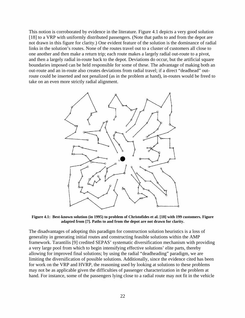
22

This notion is corroborated by evidence in the literature. Figure 4.1 depicts a very good solution [18] to a VRP with uniformly distributed passengers. (Note that paths to and from the depot are not drawn in this figure for clarity.) One evident feature of the solution is the dominance of radial links in the solution’s routes. None of the routes travel out to a cluster of customers all close to one another and then make a return trip; each route makes a largely radial out-route to a pivot, and then a largely radial in-route back to the depot. Deviations do occur, but the artificial square boundaries imposed can be held responsible for some of these. The advantage of making both an out-route and an in-route also creates deviations from radial travel; if a direct “deadhead” out-route could be inserted and not penalized (as in the problem at hand), in-routes would be freed to take on an even more strictly radial alignment.

Figure 4.1: Best-known solution (in 1995) to problem of Christofides et al. [18] with 199 customers. Figure

adapted from [7]. Paths to and from the depot are not drawn for clarity.

The disadvantages of adopting this paradigm for construction solution heuristics is a loss of generality in generating initial routes and constructing feasible solutions within the AMP framework. Tarantilis [9] credited SEPAS’ systematic diversification mechanism with providing a very large pool from which to begin intensifying effective solutions’ elite parts, thereby allowing for improved final solutions; by using the radial “deadheading” paradigm, we are limiting the diversification of possible solutions. Additionally, since the evidence cited has been for work on the VRP and HVRP, the reasoning used by looking at solutions to these problems may not be as applicable given the difficulties of passenger characterization in the problem at hand. For instance, some of the passengers lying close to a radial route may not fit in the vehicle

23

serving the route due to capacity constraints, or because adding the passenger would require the route to also visit an additional destination.

The advantage of having a framework and a vision for the solution, around which heuristics may be constructed, outweighs these disadvantages, however. This paradigm is not adopted blindly, but is backed up both by analytical work done in lower-bounding of the HVRP [4] as well as by the empirical evidence displayed above. Moreover, as will be seen, constructing algorithms to favor such a paradigm will only do so to a certain extent, and, using AMP framework, such an approach is not perfectly limiting in terms of possible solutions achieved and intensified. Moreover, some degree of simplification is desirable, since an approach that attempts to systematically handle a set of feasible routes that takes into account all or nearly all route and vehicle permutations would quickly become intractable. Also, acknowledging that the problem does include an element of quality of service for the passengers being transported, it may be noted that passengers will favor routes that take them more directly toward their destination compared to those that take them in more roundabout paths.

4.3. Weighting Passengers and Clusters

Following Bell and Wong [2], weighting of passengers is used when filling in routes in order to simplify and great speed up the insertion process. This weighting scheme takes into account peripherality, capacity requirements, mobility, and frequency of appearance in solutions, the last being a sort of empirical measure of overall difficulty of service. The use of weights helps the algorithm to satisfy those passengers most affected by constraints so that when routes are nearer to full, drastic measures need not be taken to fulfill these passengers’ demand. The weighting formula works so well that, in an empirical comparison of an exhaustive “smallest addition” insertion heuristic to one considering customers by rank, the exhaustive heuristic rarely outperformed the ranked heuristic with regards to the number of passengers satisfied by a set number of routes, while the ranked heuristic operated hundreds of times faster.

Another weighting scheme is used to evaluate routes for the AMP method used. This scores passengers only by frequency of appearance in previous solutions and mobility, emphasizing the uniqueness of fit of a route to the passengers it serves, rather than the difficulty a passenger might cause to attempts at insertion.

4.4. Vehicle Tiering

Another simplification of the complicated task of assigning vehicles to routes, vehicle tiering is used to make only the most appropriate vehicles for a given task available for assignment. Often, three tiers of vehicles are set up; a number of the most preferential vehicles are placed in the top tier, and a number of dominated or subpar vehicles are placed in the bottom tier, with the rest filling in the middle tier. When assigning a random vehicle, one is drawn first from the top tier; if using this vehicle is somehow infeasible, it is discarded and a new one is drawn from the top tier. This is repeated until a vehicle is assigned and the heuristic is terminated, or there are no vehicles left in the top tier, in which case vehicles are drawn from the middle tier, and later the bottom tier.

24

Before tiering, vehicles must somehow be ranked. As discussed in section 4.1, the configuration for vehicles is predetermined depending upon what sort of use the vehicle will have (i.e., in which run(s) it will operate). However, the multidimensionality of each vehicle’s capacity must still be accounted for – some relationship between the two capacities is needed. The parameter is proposed for the number of ambulatory seats that each wheelchair space is worth. A basis for this value can be determined by calculating the actual average trade-off between the two in convertible vehicles. For every vehicle in the set of convertible vehicles , determine maximum and minimum ambulatory capacities, and , respectively, and the maximum and minimum wheelchair capacities, respectively and . The fleet conversion trade-off value may then be calculated as

(4.1)

The value determined for may then be multiplied by a value greater than unity to favor wheelchair capacity more strongly (as in a B run assignment) or by a value less than one but greater than zero to favor ambulatory capacity more strongly (as in an A run assignment) in order to determine . Each vehicle may then be ranked based on the score , where and are the ambulatory and wheelchair capacities, respectively, of the vehicle in the given configuration.

This strategy allows for randomness in vehicle selection and assignment; rather than assigning a ranked “best” vehicle class in a first position every time, a random “good” vehicle class may be assigned in this position, increasing the diversification of solutions obtained.

5. Subroutines

A number of subroutines are used frequently in this work. A brief discussion of these follows, after which their operation will be assumed to be known. Notation is drawn from section 2.2.

5.1. Evaluate Common Route Features

Another subroutine is used, which determines salient features of a route (namely the order in which endpoints should be visited, the durations of all pick-up, drop-off, and travel operations, and, for A run routes, the length of time past 8am that the route operates) given only the sequence of nodes visited.

The subroutine accepts the sequence and a run designator; here we will use , but the same will go if a B run route is fed, with exceptions noted. In this algorithm, it is important to note that, in the A run, destination will accept passengers at any time, while the other destinations in will only accept passengers after 8am. The subroutine is given in pseudo-code in algorithm 5.1, which will be referred to in future algorithms as eval( ).

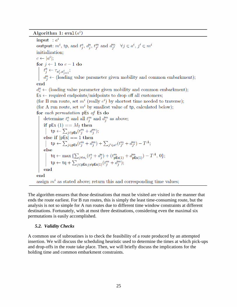
25

The algorithm ensures that those destinations that must be visited are visited in the manner that ends the route earliest. For B run routes, this is simply the least time-consuming route, but the analysis is not so simple for A run routes due to different time window constraints at different destinations. Fortunately, with at most three destinations, considering even the maximal six permutations is easily accomplished.

5.2. Validity Checks

A common use of subroutines is to check the feasibility of a route produced by an attempted insertion. We will discuss the scheduling heuristic used to determine the times at which pick-ups and drop-offs in the route take place. Then, we will briefly discuss the implications for the holding time and common embarkment constraints.

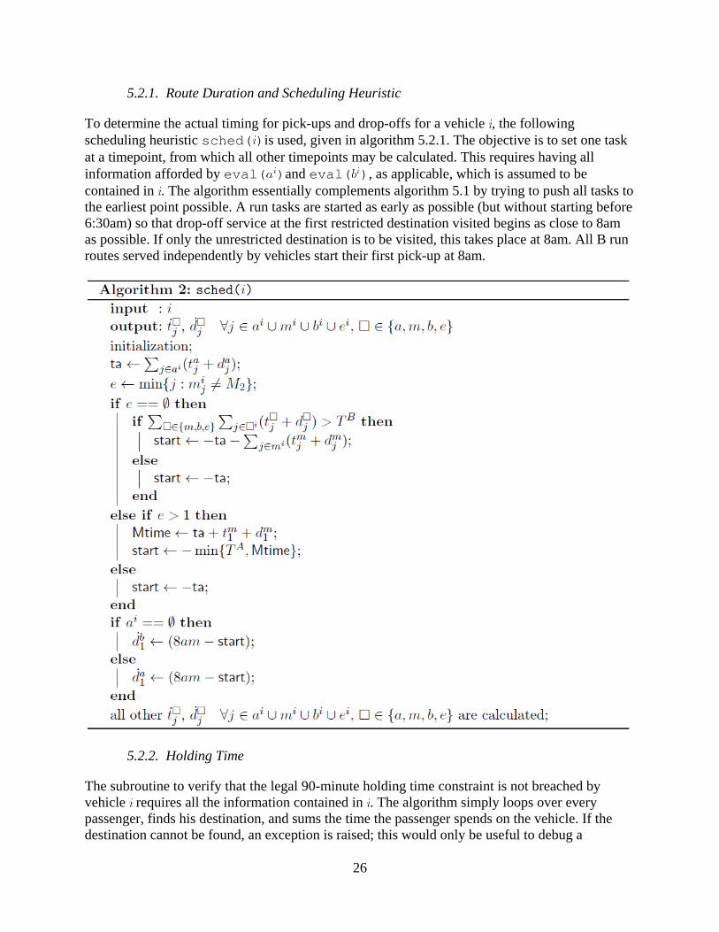
26

5.2.1. Route Duration and Scheduling Heuristic

To determine the actual timing for pick-ups and drop-offs for a vehicle , the following scheduling heuristic sched( )is used, given in algorithm 5.2.1. The objective is to set one task at a timepoint, from which all other timepoints may be calculated. This requires having all information afforded by eval( )and eval( ), as applicable, which is assumed to be contained in . The algorithm essentially complements algorithm 5.1 by trying to push all tasks to the earliest point possible. A run tasks are started as early as possible (but without starting before 6:30am) so that drop-off service at the first restricted destination visited begins as close to 8am as possible. If only the unrestricted destination is to be visited, this takes place at 8am. All B run routes served independently by vehicles start their first pick-up at 8am.

5.2.2. Holding Time

The subroutine to verify that the legal 90-minute holding time constraint is not breached by vehicle requires all the information contained in . The algorithm simply loops over every passenger, finds his destination, and sums the time the passenger spends on the vehicle. If the destination cannot be found, an exception is raised; this would only be useful to debug a

27

subroutine like eval( ), since this should add necessary destinations to the route. To err on the side of caution, the sum used extends from the timepoint at which pick-up serviced is initiated to the timepoint at which drop-off service is completed.

5.2.3. Common Embarkment Constraint

Not really a subroutine, enforcing the common embarkment constraint required a check at every attempted insertion. Because this constraint was imposed after the computational structure used was constructed, the constraint was enforced in practice by attempting to insert all customers that embark at a common location whenever any one of them attempted to embark. Because of the extra capacity this required, such “clusters” were weighted more strongly for insertion.

The function of such a check required constructing lists of passengers present in clusters and a hash table to tie passengers to clusters. This was accomplished by grouping any passengers and

such that . If “superclusters,” or groups that cannot be feasibly loaded on any vehicle, result, these are broken. If removal of any one passenger makes the cluster serviceable by some vehicle, this is done, and the passenger is no longer part of the cluster. Otherwise, the passengers that contribute most to the capacity violation are sequentially removed and added to a separate cluster, until the first cluster is serviceable. If the new cluster is unserviceable, this process is repeated until all clusters formed are serviceable. In this way, “clusters” were still treated as individual passengers, though with pick-up constraints, rather than as combined groups of passengers, as in the MINLP formulation in section 1.

5.3. Verify Vehicle

An overall check of a vehicle’s satisfaction of constraints can usefully determine the overall feasibility of an insertion or any other operation on a vehicle or its routes. Equipped with error messages for constraints that are broken, it is also useful for debugging purposes. Finally, it finds use in a final overarching verification step, since applying the test while looping over all vehicles requires only the additional checks that no vehicle class is overused, common embarkment constraints are enforced, and all passengers in both runs have been served.

Such a verification proceeds simply as a sequence of smaller verification checks. The holding time subroutine is used to verify that all required destinations are visited and that no passengers are held too long. The multi-dimensional load picked up in each run is calculated, and both are checked against the vehicle’s capacity for its given configuration. The constraint on transfer passengers is also checked. Finally, sched( )is carried out to make sure no passengers are picked up before 6:30am or dropped off after 9:30am, and that the destination time window constraints are not broken. These are all the required steps to ensure that a route fulfills all constraints.

6. Overview of Complete Algorithm

The overarching algorithm used to solve this problem is presented here in its entirety. Subsections that follow give some of the more complicated steps in greater detail.

28

1. Estimate objective function for both runs Each run is handled independently with the full vehicle pool available to it. An estimate is generated by only enforcing vehicle capacity constraints.

2. Serve all handicapped A run passengers Consider only nonambulatory A run passengers. Starting with the most peripheral of these, construct a route by “smallest additions” principle discussed in section 2.4. Repeat this until all nonambulatory A run passengers are served.

3. Serve as many B run passengers as possible with those vehicles List the number of vehicles available at each A run destination, and serve passenger clusters requiring maximum wheelchair capacity first. Generate a set of 3 3 matrices that describe which A run destination and B run destination vehicles will visit. For each matrix, serve as many nonambulatory B run passengers as possible, then calculate total wheelchair capacity used and how total route slack time remaining. Choosing the matrix (and related routes) that produces the greatest weighted sum of these values, assign vehicles to A run routes first by necessity and then matching excess capacity to slack time. Match B run routes to these using a simple heuristic.

4. Exhaustively fill in two-run routes with ambulatory passengers Search for the combination of run, route, passenger, and position that creates the smallest addition to total time the selected vehicle spends serving both routes. Insert passengers in this manner until no more can be inserted.

5. Solve remaining A and B runs separately with Decrementing Adaptive Memory Program (DAMP) For each run: set based on estimate; initialize preset, score ; do{ (a) Assign starting passengers, vehicles Initiate routes with each of the passengers in

preset and assign vehicles accordingly, as able. Probabilistically select other starting passengers, favoring those that are most peripheral, until routes have been formed. Assign vehicles by tiers to these in a random manner.

(b) Complete routes by filling in Weight unserved passengers in the run with respect to peripherality, capacity requirements, mobility, and frequency of appearance in previous solutions. Working down the list of passengers hardest to serve, find the smallest addition into any position in any route, and insert the passenger as possible. Repeat this until the list is exhausted.

(c) If satisfied, decrement number of starts If every passenger is served, store the solution as the best found so far, set and preset, score , then go to (a).

(d) If incomplete, evaluate solution achieved Weight passengers as a function of frequency of appearance in previous solutions and mobility. For each route served by a single-run vehicle, sum the weights of the passengers served, and update with a new or updated entry for the starting passenger and vehicle used for that route.

(e) Weigh inputs based on outputs and loop Select and assign preset (top highest-scored starting passenger-vehicle combinations), where is a function of and the number of passengers served in the last attempt.

} while (number of iterations without decrement maximum number of iterations)

This algorithm seeks to partition the problem into three parts. The first part is the small nonambulatory A run population. These will be served by high wheelchair capacity vehicles so as to minimize the number of routes used. Since high-capacity vehicles are used, they will continue on to serve B run passengers, but since these B run routes will be constrained in time,

29

these vehicles should be assigned to nonambulatory B run passengers near the destinations. This will allow them to serve more passengers in a shorter time; other B run routes can serve customers that are farther out.

The remaining populations are ambulatory A run passengers and more peripheral B run passengers. These are handled separately but similarly; the Decrementing Adaptive Memory Program (DAMP) attempts to form radially-aligned routes to serve each of these populations. It does so by keeping a memory of passengers and vehicles with which it starts routes, and scoring these combinations based on the quality of the route they produce when filled in.

The details of this algorithm will be expanded upon in the ensuing subsections, the numbers of which correspond to the step in the list above.

6.1. Estimate Objective Function Value for both Runs

A rough lower bound may be generated by enforcing only vehicle constraints. Such a lower bound may be useful for measuring the effectiveness of the algorithm. In this case, an approximation of this lower bound will be used to estimate how many routes are needed to serve all the passengers for each run. Since the number will only be used as the basis of an estimate, emphasis is placed on finding this estimate cheaply rather than accurately, and the method presented here actually gives a small overestimation of a fairly loose lower bound. The following algorithm establishes the required capacity of a run as a vector and considers vehicles as smaller vectors, which can be added to a value equal to or greater than the former vector in both the ambulatory and wheelchair capacity dimensions.

1. Initiate target vector. Sum the amount of each type of capacity needed and store as target. Set .

do{

2. Determine best vehicle and configuration available. Search through vehicles (in both configurations) to find the vehicle with capacity vcap which minimizes

. If a vehicle is found which has more capacity in both dimensions than target, select this vehicle automatically.

3. Reduce target. . 4. Remove vehicle from pool. Also set .

} while (at least one entry of )

This is a greedy method and, in the case study examined, tends to overshoot the actual lower bound slightly. In seeking to minimize the norm, the algorithm will use high ambulatory capacity vehicles early on, overshooting the amount of ambulatory capacity assigned since many vehicles have more ambulatory capacity than wheelchair capacity, even in configurations that maximize wheelchair capacity. In practice, this overestimation was by 8% or less for both runs.

Overall, since this lower bound ignores many constraints on timing, precedence, and common embarkment, it is acknowledged to be somewhat loose to begin with, so a slight overestimation is acceptable. This estimate will be used in step 5.

30

6.2. Serve all Handicapped A Run Passengers

This is the first part of the actual solution algorithm. Limiting the population to nonambulatory A run passengers, high-capacity vehicles are used to form radially-aligned “deadhead” routes sequentially, constructing each one by starting at a peripheral customer and adding passengers who do not significantly increase the vehicle’s travel time. The efficiency of the algorithm in solving this problem with the minimum number of routes is not of highest importance, since these vehicles will be able to serve both the remaining A and B run populations as well; this idea is drawn from the discussion in section 2.3 regarding the usefulness of high-capacity vehicles to serve both populations. Due to the time constraints imposed by such an assignment, the best way to make use of these high capacities is to serve passengers nearby one another and their destinations, which is what is done in the next step.

In the following, let represent the set of nonambulatory A run passengers. The heuristic takes the following form:

1. Initialize. List vehicles, ranked first by wheelchair capacity, then by ambulatory capacity.

do{

2. Pick a starting passenger such that . Assign this passenger a route, served by the top vehicle on the list.

3. Build a route. Add any passengers that must embark at the same location as the starting passenger to the route and add all passengers in the route to . Then do{ (a) Exclude ineligible passengers. These include those for whose load the vehicle has

insufficient remaining capacity, including considerations of common embarkment, or any incompatibilities between mobility type and vehicle class.

Let = {all eligible passengers }. Initialize memory to record the best solution. Then, for all , { and

for all possible insertion positions , {

(b) Run eval( ), where is the route with the addition of (and any necessary other clustered passengers) in position . Check that is a valid route, and if not, go to the next iteration.

(c) Score the addition. Determine the time required to run the route, minus the embarkment time for and its clustered passengers, if any. If this is better (less) than the best duration found so far, record the value as well as and .

} }

(d) Finalize the insertion. Insert and clustered passengers, if any, in , and add them to . If no valid insertion was found, insert none.

} while (some valid insertion was found last iteration)

4. Verify and save the route. Remove the assigned vehicle from the list.

31

} while ( , where refers to a proper subset)

This algorithm works in a straightforward manner, but a few details deserve discussion. The vehicle tiering discussed in section 4.4 is not used because vehicle assignments are not yet firm. The vehicles highest in wheelchair capacity are used first, and these will be assigned to routes in the next step, when routes are matched with B run routes. Also, the search for smallest additions is exhaustive at every step. This is reasonable since the population considered, nonambulatory A run passengers, is small. It would be possible, if this were prohibitively expensive, to grab only a couple dozen passengers to consider, for example by ranking all by the size of the ellipse centered on the two closest nodes of passengers in the route needed to contain , and selecting the 20 or so passengers with the smallest required ellipses.

The scoring method in step 3(c) may also provoke questions. Omitting embarkment duration from the score causes only the additional travel time, as well as any additional time spent in the drop-off phase, to be considered. This is beneficial, as otherwise, passengers with lower embarkment times receive a sort of unmerited award. Indeed, this could cause passengers or passenger clusters that would already be difficult to serve additional difficulties due to increased competition for capacity on nearby routes from low-embarkment-duration passengers. This embarkment time must be accounted for, whether by one vehicle or another; there is no way to reduce it or escape it, and if it proves to cause the route to break time constraints, the insertion will not pass verification and therefore will not be recorded.

After this is accomplished, a set of routes exist that serve all nonambulatory (and only nonambulatory) A run passengers, each route ideally serving several passengers depending on the exact makeup of the problem and the vehicles available. The next step is to take the results of this analysis and route these vehicles from the A run destinations that complete their A run routes to pick up B run passengers.

6.3. Serve Nonambulatory B Run Passengers with those Vehicles

In order to serve as many nonambulatory B run passengers as possible, each vehicle, continuing into the B run from its A run route in the previous solution, is initially limited to picking up nonambulatory B run passengers with a common destination, to avoid spending time visiting multiple destinations. The problem then becomes one of matching vehicles that have just completed routes at A run destinations with a target B run destination. Once a good approximation is made for this, B run routes are constructed and then matched to corresponding A run routes. This step will be broken into two parts: first, a number of combinations of A run destinations with B run destinations will be generated and scored; second, the highest-scoring combination is selected, and then actual B run routes are formed in the same quantity as the A run routes, and matched to these.

In the following, let represent the set of nonambulatory B run passengers. Final A run destinations for the routes generated in section 6.2 will be referred to as “midpoints” and B run destinations as “endpoints.” The heuristic takes the following form:

32

6.3.1. Generate Combinations of Midpoints and Endpoints

1. Count vehicles available at each midpoints, regardless of the time at which service is completed.

2. Assign B run clusters to a midpoint. For passengers in clusters larger than or equal to a specified size, determine the nearest midpoint with available vehicles. Create a B run route with the passengers in the cluster, add these passengers to , label this route with the chosen midpoint, and remove one vehicle from the midpoint.

3. Initialize memory for search and scoring. Start with , and initialize memory for two metrics, load and ftb.

do{

4. Generate an s-t matrix, or a 3 3 matrix where entries are the number of vehicles traveling from midpoint to endpoint , excluding those considered in step 2. Initialize and an empty 3 3 matrix and do{ (a) Determine the eligible passenger nearest any midpoint with at least

one available vehicle. (b) Assign the vehicle from its midpoint to the endpoint that is . Remove that vehicle

from availability and increment the corresponding entry in the s-t matrix. (c) Remove a handful of passengers. Considering only the subset such that

and , add the passengers nearest to to .

} while (at least one vehicle still needs to be assigned)

5. Assign passengers to routes with the goal of assigning nearby nonambulatory passengers of common destination to common routes. Given the s-t matrix, for all , { and for all such that at least one vehicle needs a route, { (a) Rank eligible passengers. Considering only the subset such that

and , rank all passengers in ascending order of the sum of .

(b) Select and label passengers. Given the capacity of vehicles available at , sequentially add passengers from the top of the list into set until the load exceeds this capacity. Label all of these passengers by the difference . Then,

do{

(c) Select starting passenger with the smallest label. (d) Build a route from the starting passenger, just as in step 3 of the algorithm on page

31, though with the current definition of . (e) Finalize route. Label this route with its midpoint, and add all passengers in it to .

} while (at least one vehicle at still needs to be routed)

}}

33

6. Score and save solution. Each route’s ftb_route is calculated as (the total time needed to run the route, starting at the labeled midpoint). If, for any route, this is less than the minimum time any A run route operates after 8am, invalidate this solution and break the loop. Otherwise, store the solution and two metrics: its ftb, the sum of all route ftb_route values, and its load, the amount of ambulatory capacity consumed by passengers.

7. Increment h.

} while (previous solution was valid)

Timing is disregarded in step 1, as this will be addressed during the matching of A run routes to the B run routes generated here. In step 2, the cut-off size of clusters automatically assigned should be tailored to the problem based on the number and size of passenger clusters present and the availability of vehicles to serve these clusters. In the case study, only those (four) clusters with the maximum possible wheelchair load (5) were automatically assigned. This assignment ensures that these passengers, whose demand is very difficult to meet otherwise, are served by high-capacity vehicles. Additionally, since this service requires visiting only one node, the vehicle is free to pick up more ambulatory passengers, as discussed in the next section.

The search over parameter has been constructed as a way of generating reasonable s-t matrices. Passengers near the midpoints are greedily assigned, and represents the number of passengers of common destination nearest that midpoint that are considered “served” by that vehicle assignment. Since in the next step, routes are actually formed from these passengers, it is reasonable to assume that a number of nearby eligible passengers will be served. In other words, the disqualification of nearby passengers is a stand-in in anticipation of actual service by a vehicle. In fact, such a strategy of greedy search and disqualification is only a means of generating an s-t matrix for step 5, but when its function is understood as a sort of “surrogate assignment,” such a strategy becomes reasonable for generating a small but good set of matrices to score.

Actual route assignments, then proceed by the previously discussed method of smallest additions. The partitioning of the population that occurs when is constructed is meant to keep these routes near the problem’s central area, and is especially focused on the area between and around the midpoint and endpoint between which the route will run. It may be possible to serve more passengers by relaxing this partition, but the goal is not solely to serve nonambulatory passengers with these routes. Ambulatory passengers will be added in a later step, and a benefit of not allowing these routes to spread out too far is the slack time, available for serving ambulatory passengers, present in a route that is spatially contained. Since these routes are built sequentially, they are started at a node that is close to the origin (midpoint) and far from the destination (endpoint), which is the purpose of the passenger’s label.

Along the same line, the score assigned to the solution for a given value of includes two metrics: load, a measure of how well the solution does its job of serving nonambulatory passengers, and ftb_route, a measure of how efficiently it does this job and, likewise, its potential ability to serve ambulatory passengers in the next phase.

34

These scores will be used to select one of the solutions generated, the routes of which will then be matched to A run routes with a matching a midpoint. Vehicle classes are assigned to A run routes, and matching of B run routes occurs by first satisfying needs with regards to capacity, then attempting to assign B run routes with the greatest values of ftb to the highest capacity vehicles.

6.3.2. Select Solution and Solve Route-Matching and Vehicle Assignment Problem

1. Take the highest-scoring solution. Solutions are scored by the sum , where is the tradeoff value of a space of wheelchair capacity in minutes of operating time. A value of 6 minutes was used in the case study. The solution with the highest score is selected.

2. Calculate for each A run route: aload, the ambulatory load on the route (since transfer passengers require ambulatory capacity, and some ambulatory passengers may be in routes due to common embarkment with wheelchair passengers); tp8, the time past 8am the route requires to drop off its last A run passenger; and fta, calculated as (time needed from initiating first pick-up to beginning disembarking at first destination).

3. Rank the vehicles in the configuration that maximizes wheelchair capacity, first by wheelchair capacity, then by ambulatory capacity. Consider for assignment the same number as there are A run routes (and B run routes), taken from the top of the list, and place these in set .

for all A run routes, {

4. If the route has aload , assign to it the vehicle with the smallest feasible capacity.

}

5. Assign the other vehicles to A run routes such that the routes with the highest values of fta get the highest ambulatory capacity vehicles. With each A run route assigned a vehicle, label the routes with acap, the ambulatory capacity of the vehicle.

for all , {

6. Rank routes. Consider only those routes labeled with midpoint . Of these, rank the routes from different runs, the A run routes by the value of acap and the B run routes by the value of ftb.

7. Construct feasible matching matrix, which has entries , where if the (ftb of the -ranked B route) (tp8 of the -ranked A route), and 0 otherwise. Each matrix row describes the feasibility of matching a B run route with each A run route, where rows and columns are ordered by the ranks of the previous step.

8. Assign B run routes to A run routes using the feasible matching matrix, with the rule that the B run route with the highest ftb is to be matched with the A run route with the highest ftb, given that all routes are paired. If the entry of the assignment matrix , this indicates that the -ranked B route is matched to the -ranked A route. Assignment

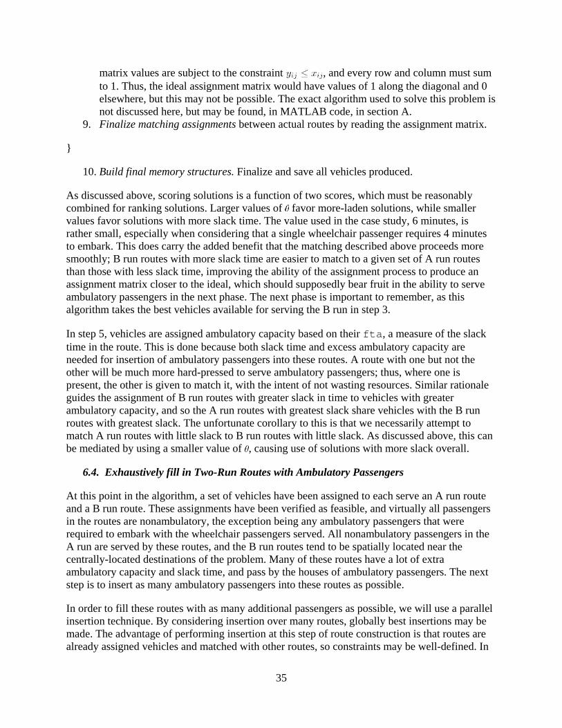
35

matrix values are subject to the constraint , and every row and column must sum to 1. Thus, the ideal assignment matrix would have values of 1 along the diagonal and 0 elsewhere, but this may not be possible. The exact algorithm used to solve this problem is not discussed here, but may be found, in MATLAB code, in section A.

9. Finalize matching assignments between actual routes by reading the assignment matrix.

}

10. Build final memory structures. Finalize and save all vehicles produced.

As discussed above, scoring solutions is a function of two scores, which must be reasonably combined for ranking solutions. Larger values of favor more-laden solutions, while smaller values favor solutions with more slack time. The value used in the case study, 6 minutes, is rather small, especially when considering that a single wheelchair passenger requires 4 minutes to embark. This does carry the added benefit that the matching described above proceeds more smoothly; B run routes with more slack time are easier to match to a given set of A run routes than those with less slack time, improving the ability of the assignment process to produce an assignment matrix closer to the ideal, which should supposedly bear fruit in the ability to serve ambulatory passengers in the next phase. The next phase is important to remember, as this algorithm takes the best vehicles available for serving the B run in step 3.

In step 5, vehicles are assigned ambulatory capacity based on their fta, a measure of the slack time in the route. This is done because both slack time and excess ambulatory capacity are needed for insertion of ambulatory passengers into these routes. A route with one but not the other will be much more hard-pressed to serve ambulatory passengers; thus, where one is present, the other is given to match it, with the intent of not wasting resources. Similar rationale guides the assignment of B run routes with greater slack in time to vehicles with greater ambulatory capacity, and so the A run routes with greatest slack share vehicles with the B run routes with greatest slack. The unfortunate corollary to this is that we necessarily attempt to match A run routes with little slack to B run routes with little slack. As discussed above, this can be mediated by using a smaller value of , causing use of solutions with more slack overall.

6.4. Exhaustively fill in Two-Run Routes with Ambulatory Passengers

At this point in the algorithm, a set of vehicles have been assigned to each serve an A run route and a B run route. These assignments have been verified as feasible, and virtually all passengers in the routes are nonambulatory, the exception being any ambulatory passengers that were required to embark with the wheelchair passengers served. All nonambulatory passengers in the A run are served by these routes, and the B run routes tend to be spatially located near the centrally-located destinations of the problem. Many of these routes have a lot of extra ambulatory capacity and slack time, and pass by the houses of ambulatory passengers. The next step is to insert as many ambulatory passengers into these routes as possible.

In order to fill these routes with as many additional passengers as possible, we will use a parallel insertion technique. By considering insertion over many routes, globally best insertions may be made. The advantage of performing insertion at this step of route construction is that routes are already assigned vehicles and matched with other routes, so constraints may be well-defined. In

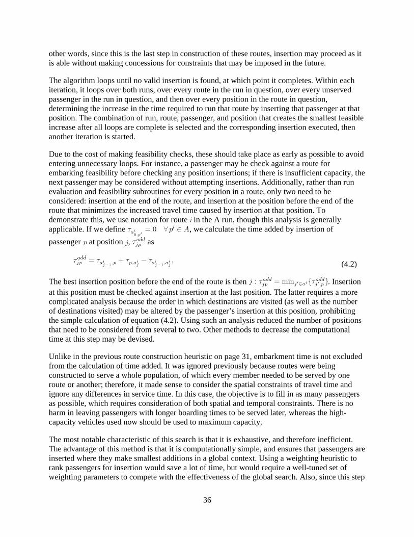
36

other words, since this is the last step in construction of these routes, insertion may proceed as it is able without making concessions for constraints that may be imposed in the future.

The algorithm loops until no valid insertion is found, at which point it completes. Within each iteration, it loops over both runs, over every route in the run in question, over every unserved passenger in the run in question, and then over every position in the route in question, determining the increase in the time required to run that route by inserting that passenger at that position. The combination of run, route, passenger, and position that creates the smallest feasible increase after all loops are complete is selected and the corresponding insertion executed, then another iteration is started.

Due to the cost of making feasibility checks, these should take place as early as possible to avoid entering unnecessary loops. For instance, a passenger may be check against a route for embarking feasibility before checking any position insertions; if there is insufficient capacity, the next passenger may be considered without attempting insertions. Additionally, rather than run evaluation and feasibility subroutines for every position in a route, only two need to be considered: insertion at the end of the route, and insertion at the position before the end of the route that minimizes the increased travel time caused by insertion at that position. To demonstrate this, we use notation for route in the A run, though this analysis is generally applicable. If we define , we calculate the time added by insertion of passenger at position , as

(4.2)

The best insertion position before the end of the route is then . Insertion at this position must be checked against insertion at the last position. The latter requires a more complicated analysis because the order in which destinations are visited (as well as the number of destinations visited) may be altered by the passenger’s insertion at this position, prohibiting the simple calculation of equation (4.2). Using such an analysis reduced the number of positions that need to be considered from several to two. Other methods to decrease the computational time at this step may be devised.

Unlike in the previous route construction heuristic on page 31, embarkment time is not excluded from the calculation of time added. It was ignored previously because routes were being constructed to serve a whole population, of which every member needed to be served by one route or another; therefore, it made sense to consider the spatial constraints of travel time and ignore any differences in service time. In this case, the objective is to fill in as many passengers as possible, which requires consideration of both spatial and temporal constraints. There is no harm in leaving passengers with longer boarding times to be served later, whereas the high-capacity vehicles used now should be used to maximum capacity.

The most notable characteristic of this search is that it is exhaustive, and therefore inefficient. The advantage of this method is that it is computationally simple, and ensures that passengers are inserted where they make smallest additions in a global context. Using a weighting heuristic to rank passengers for insertion would save a lot of time, but would require a well-tuned set of weighting parameters to compete with the effectiveness of the global search. Also, since this step

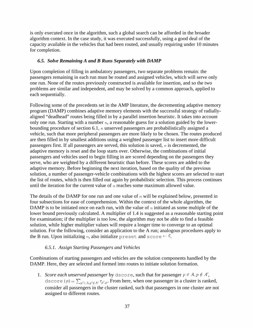
37

is only executed once in the algorithm, such a global search can be afforded in the broader algorithm context. In the case study, it was executed successfully, using a good deal of the capacity available in the vehicles that had been routed, and usually requiring under 10 minutes for completion.

6.5. Solve Remaining A and B Runs Separately with DAMP

Upon completion of filling in ambulatory passengers, two separate problems remain: the passengers remaining in each run must be routed and assigned vehicles, which will serve only one run. None of the routes previously constructed is available for insertion, and so the two problems are similar and independent, and may be solved by a common approach, applied to each sequentially.

Following some of the precedents set in the AMP literature, the decrementing adaptive memory program (DAMP) combines adaptive memory elements with the successful strategy of radially-aligned “deadhead” routes being filled in by a parallel insertion heuristic. It takes into account only one run. Starting with a number , a reasonable guess for a solution guided by the lower-bounding procedure of section 6.1, unserved passengers are probabilistically assigned a vehicle, such that more peripheral passengers are more likely to be chosen. The routes produced are then filled in by smallest additions using a weighted passenger list to insert more difficult passengers first. If all passengers are served, this solution is saved, is decremented, the adaptive memory is reset and the loop starts over. Otherwise, the combinations of initial passengers and vehicles used to begin filling in are scored depending on the passengers they serve, who are weighted by a different heuristic than before. These scores are added to the adaptive memory. Before beginning the next iteration, based on the quality of the previous solution, a number of passenger-vehicle combinations with the highest scores are selected to start the list of routes, which is then filled out again by probabilistic selection. This process continues until the iteration for the current value of reaches some maximum allowed value.

The details of the DAMP for one run and one value of will be explained below, presented in four subsections for ease of comprehension. Within the context of the whole algorithm, the DAMP is to be initiated once on each run, with the value of initiated as some multiple of the lower bound previously calculated. A multiplier of 1.4 is suggested as a reasonable starting point for examination; if the multiplier is too low, the algorithm may not be able to find a feasible solution, while higher multiplier values will require a longer time to converge to an optimal solution. For the following, consider an application to the A run; analogous procedures apply to the B run. Upon initializing , also initialize preset and score .

6.5.1. Assign Starting Passengers and Vehicles

Combinations of starting passengers and vehicles are the solution components handled by the DAMP. Here, they are selected and formed into routes to initiate solution formation.

1. Score each unserved passenger by dscore, such that for passenger , dscore( ) . From here, when one passenger in a cluster is ranked, consider all passengers in the cluster ranked, such that passengers in one cluster are not assigned to different routes.

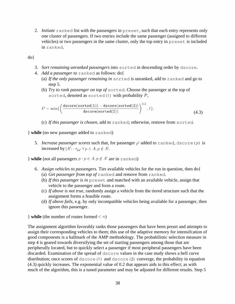
38

2. Initiate ranked list with the passengers in preset, such that each entry represents only one cluster of passengers. If two entries include the same passenger (assigned to different vehicles) or two passengers in the same cluster, only the top entry in preset is included in ranked.

do{

3. Sort remaining unranked passengers into sorted in descending order by dscore. 4. Add a passenger to ranked as follows: do{

(a) If the only passenger remaining in sorted is unranked, add to ranked and go to step 5.

(b) Try to rank passenger on top of sorted. Choose the passenger at the top of sorted, denoted as sorted( ) with probability ,

(4.3)

(c) If this passenger is chosen, add to ranked; otherwise, remove from sorted.

} while (no new passenger added to ranked)

5. Increase passenger scores such that, for passenger added to ranked, dscore( ) is increased by .

} while (not all passengers are in ranked)

6. Assign vehicles to passengers. Tier available vehicles for the run in question, then do{ (a) Get passenger from top of ranked and remove from ranked. (b) If this passenger is in preset and matched with an available vehicle, assign that

vehicle to the passenger and form a route. (c) If above is not true, randomly assign a vehicle from the tiered structure such that the

assignment forms a feasible route. (d) If above fails, e.g. by only incompatible vehicles being available for a passenger, then

ignore this passenger.

} while (the number of routes formed )

The assignment algorithm favorably ranks those passengers that have been preset and attempts to assign their corresponding vehicles to them; this use of the adaptive memory for intensifcation of good components is a hallmark of the AMP methodology. The probabilistic selection measure in step 4 is geared towards diversifying the set of starting passengers among those that are peripherally located, but to quickly select a passenger if most peripheral passengers have been discarded. Examination of the spread of dscore values in the case study shows a bell curve distribution; once scores of dscore( ) and dscore( ) converge, the probability in equation (4.3) quickly increases. The exponential value of 0.2 that appears aids in this effect; as with much of the algorithm, this is a tuned parameter and may be adjusted for different results. Step 5

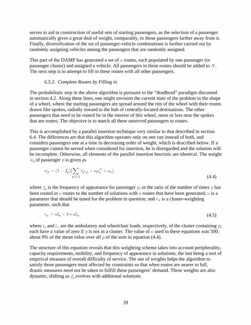
39

serves to aid in construction of useful sets of starting passengers, as the selection of a passenger automatically gives a great deal of weight, comparably, to those passengers farther away from it. Finally, diversification of the set of passenger-vehicle combinations is further carried out by randomly assigning vehicles among the passengers that are randomly assigned.

This part of the DAMP has generated a set of routes, each populated by one passenger (or passenger cluster) and assigned a vehicle. All passengers in these routes should be added to . The next step is to attempt to fill in these routes with all other passengers.

6.5.2. Complete Routes by Filling in

The probabilistic step in the above algorithm is pursuant to the “deadhead” paradigm discussed in section 4.2. Along these lines, one might envision the current state of the problem in the shape of a wheel, where the starting passengers are spread around the rim of the wheel with their routes drawn like spokes, radially inward to the hub of centrally-located destinations. The other passengers that need to be routed lie in the interior of this wheel, more or less near the spokes that are routes. The objective is to match all these unserved passengers to routes.

This is accomplished by a parallel insertion technique very similar to that described in section 6.4. The differences are that this algorithm operates only on one run instead of both, and considers passengers one at a time in decreasing order of weight, which is described below. If a passenger cannot be served when considered for insertion, he is disregarded and the solution will be incomplete. Otherwise, all elements of the parallel insertion heuristic are identical. The weight

of passenger is given as

(4.4)

where is the frequency of appearance for passenger , or the ratio of the number of times has been routed in routes to the number of solutions with routes that have been generated; is a parameter that should be tuned for the problem in question; and is a cluster-weighting parameter, such that

(4.5)

where and are the ambulatory and wheelchair loads, respectively, of the cluster containing ; each have a value of zero if is not in a cluster. The value of used in these equations was 500, about 9% of the mean value over all of the sum in equation (4.4).

The structure of this equation reveals that this weighting scheme takes into account peripherality, capacity requirements, mobility, and frequency of appearance in solutions, the last being a sort of empirical measure of overall difficulty of service. The use of weights helps the algorithm to satisfy those passengers most affected by constraints so that when routes are nearer to full, drastic measures need not be taken to fulfill these passengers’ demand. These weights are also dynamic, shifting as evolves with additional solutions.

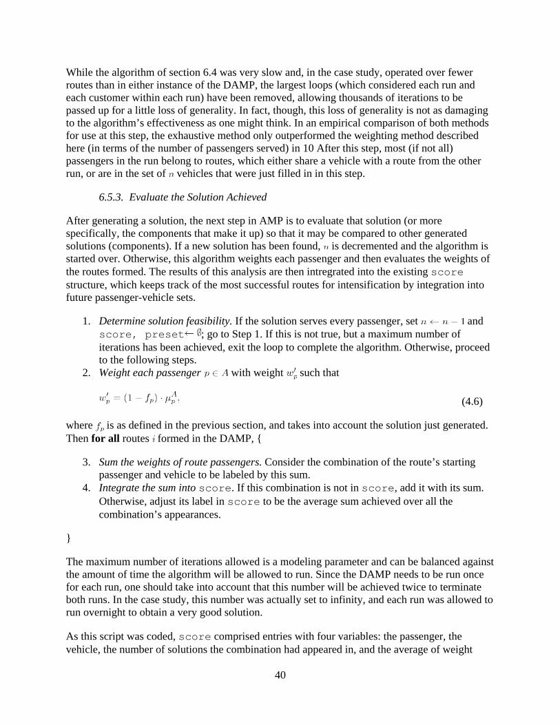
40

While the algorithm of section 6.4 was very slow and, in the case study, operated over fewer routes than in either instance of the DAMP, the largest loops (which considered each run and each customer within each run) have been removed, allowing thousands of iterations to be passed up for a little loss of generality. In fact, though, this loss of generality is not as damaging to the algorithm’s effectiveness as one might think. In an empirical comparison of both methods for use at this step, the exhaustive method only outperformed the weighting method described here (in terms of the number of passengers served) in 10 After this step, most (if not all) passengers in the run belong to routes, which either share a vehicle with a route from the other run, or are in the set of vehicles that were just filled in in this step.

6.5.3. Evaluate the Solution Achieved

After generating a solution, the next step in AMP is to evaluate that solution (or more specifically, the components that make it up) so that it may be compared to other generated solutions (components). If a new solution has been found, is decremented and the algorithm is started over. Otherwise, this algorithm weights each passenger and then evaluates the weights of the routes formed. The results of this analysis are then intregrated into the existing score structure, which keeps track of the most successful routes for intensification by integration into future passenger-vehicle sets.

1. Determine solution feasibility. If the solution serves every passenger, set and score, preset ; go to Step 1. If this is not true, but a maximum number of iterations has been achieved, exit the loop to complete the algorithm. Otherwise, proceed to the following steps.

2. Weight each passenger with weight such that

(4.6)

where is as defined in the previous section, and takes into account the solution just generated. Then for all routes formed in the DAMP, {

3. Sum the weights of route passengers. Consider the combination of the route’s starting passenger and vehicle to be labeled by this sum.

4. Integrate the sum into score. If this combination is not in score, add it with its sum. Otherwise, adjust its label in score to be the average sum achieved over all the combination’s appearances.

}

The maximum number of iterations allowed is a modeling parameter and can be balanced against the amount of time the algorithm will be allowed to run. Since the DAMP needs to be run once for each run, one should take into account that this number will be achieved twice to terminate both runs. In the case study, this number was actually set to infinity, and each run was allowed to run overnight to obtain a very good solution.

As this script was coded, score comprised entries with four variables: the passenger, the vehicle, the number of solutions the combination had appeared in, and the average of weight

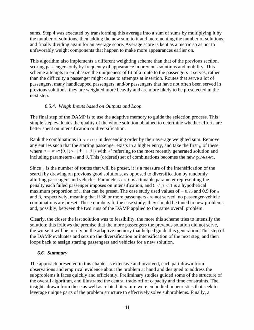
41

sums. Step 4 was executed by transforming this average into a sum of sums by multiplying it by the number of solutions, then adding the new sum to it and incrementing the number of solutions, and finally dividing again for an average score. Average score is kept as a metric so as not to unfavorably weight components that happen to make more appearances earlier on.

This algorithm also implements a different weighting scheme than that of the previous section, scoring passengers only by frequency of appearance in previous solutions and mobility. This scheme attempts to emphasize the uniqueness of fit of a route to the passengers it serves, rather than the difficulty a passenger might cause to attempts at insertion. Routes that serve a lot of passengers, many handicapped passengers, and/or passengers that have not often been served in previous solutions, they are weighted more heavily and are more likely to be preselected in the next step.

6.5.4. Weigh Inputs based on Outputs and Loop

The final step of the DAMP is to use the adaptive memory to guide the selection process. This simple step evaluates the quality of the whole solution obtained to determine whether efforts are better spent on intensification or diversification.

Rank the combinations in score in descending order by their average weighted sum. Remove any entries such that the starting passenger exists in a higher entry, and take the first of these, where with referring to the most recently generated solution and including parameters and . This (ordered) set of combinations becomes the new preset.

Since is the number of routes that will be preset, it is a measure of the intensification of the search by drawing on previous good solutions, as opposed to diversification by randomly allotting passengers and vehicles. Parameter is a tunable parameter representing the penalty each failed passenger imposes on intensification, and is a hypothetical maximum proportion of that can be preset. The case study used values of and 0.9 for and , respectively, meaning that if 36 or more passengers are not served, no passenger-vehicle combinations are preset. These numbers fit the case study; they should be tuned to new problems and, possibly, between the two runs of the DAMP applied to the same overall problem.

Clearly, the closer the last solution was to feasibility, the more this scheme tries to intensify the solution; this follows the premise that the more passengers the previous solution did not serve, the worse it will be to rely on the adaptive memory that helped guide this generation. This step of the DAMP evaluates and sets up the diversification or intensification of the next step, and then loops back to assign starting passengers and vehicles for a new solution.

6.6. Summary

The approach presented in this chapter is extensive and involved, each part drawn from observations and empirical evidence about the problem at hand and designed to address the subproblems it faces quickly and efficiently. Preliminary studies guided some of the structure of the overall algorithm, and illustrated the central trade-off of capacity and time constraints. The insights drawn from these as well as related literature were embodied in heuristics that seek to leverage unique parts of the problem structure to effectively solve subproblems. Finally, a

42

detailed description of the algorithm, from its subroutines through its overarching structure was given. The five-step algorithm was explained and the DAMP was proposed as an effective method for solving the fifth (and largest) step.

While metrics may be drawn up to analyze the function of many parts of this algorithm, the most relevant test it faces is to generate a solution for an instance of the problem at hand. The success of this algorithm depends upon the quality of the solution achieved. Presentation of this solution, and a discussion of its qualities, is the purpose of the next chapter.

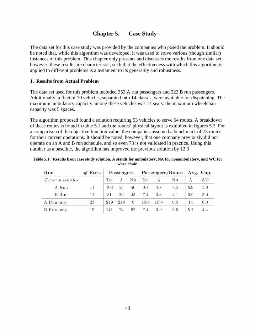
43

Chapter 5. Case Study

The data set for this case study was provided by the companies who posed the problem. It should be noted that, while this algorithm was developed, it was used to solve various (though similar) instances of this problem. This chapter only presents and discusses the results from one data set; however, these results are characteristic, such that the effectiveness with which this algorithm is applied to different problems is a testament to its generality and robustness.

1. Results from Actual Problem

The data set used for this problem included 352 A run passengers and 222 B run passengers. Additionally, a fleet of 70 vehicles, separated into 14 classes, were available for dispatching. The maximum ambulatory capacity among these vehicles was 14 seats; the maximum wheelchair capacity was 5 spaces.

The algorithm proposed found a solution requiring 53 vehicles to serve 64 routes. A breakdown of these routes is found in table 5.1 and the routes’ physical layout is exhibited in figures 5.2. For a comparison of the objective function value, the companies assumed a benchmark of 73 routes for their current operations. It should be noted, however, that one company previously did not operate on an A and B run schedule, and so even 73 is not validated in practice. Using this number as a baseline, the algorithm has improved the previous solution by 12.3

Table 5.1: Results from case study solution. A stands for ambulatory, NA for nonambulatory, and WC for wheelchair.

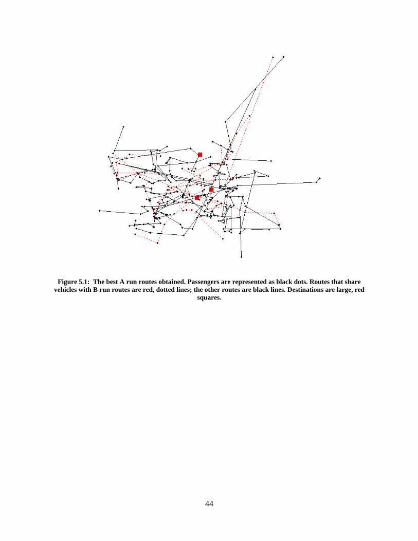
44

Figure 5.1: The best A run routes obtained. Passengers are represented as black dots. Routes that share

vehicles with B run routes are red, dotted lines; the other routes are black lines. Destinations are large, red squares.

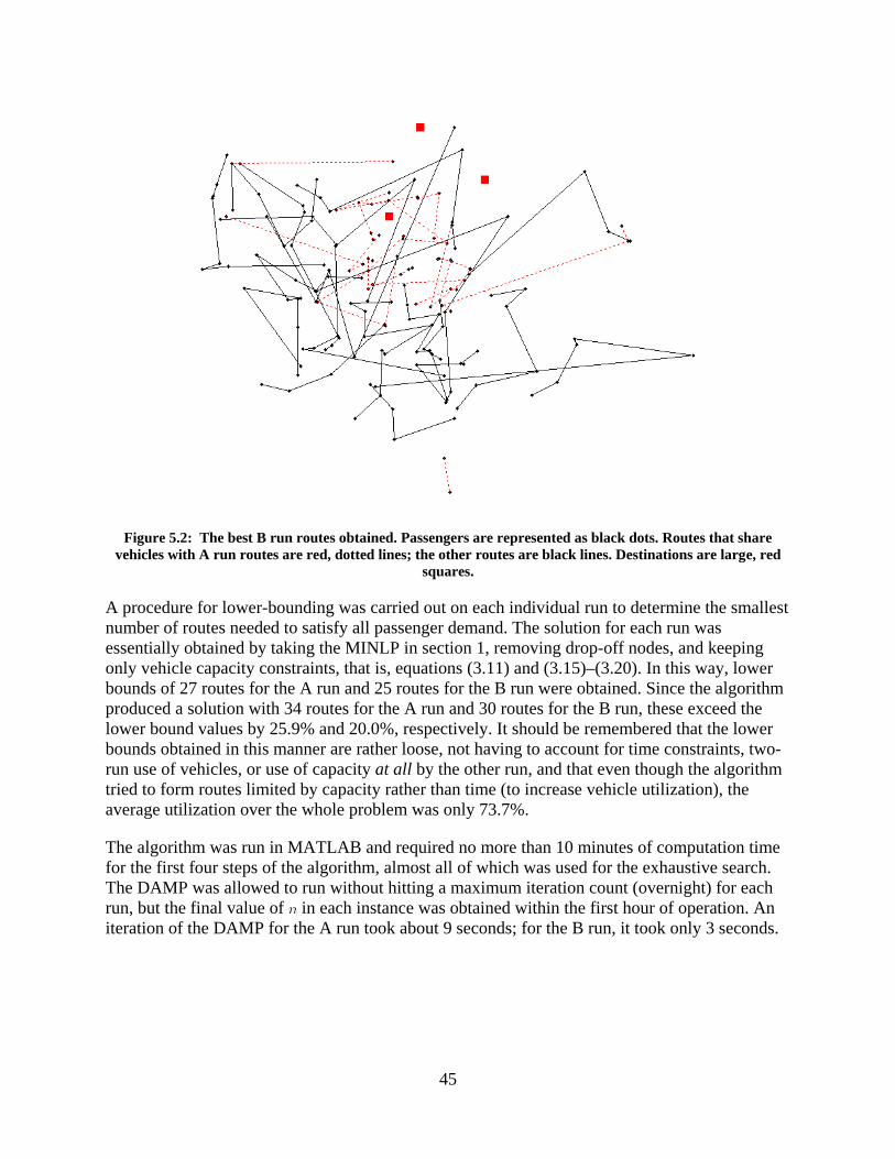
45

Figure 5.2: The best B run routes obtained. Passengers are represented as black dots. Routes that share vehicles with A run routes are red, dotted lines; the other routes are black lines. Destinations are large, red

squares.

A procedure for lower-bounding was carried out on each individual run to determine the smallest number of routes needed to satisfy all passenger demand. The solution for each run was essentially obtained by taking the MINLP in section 1, removing drop-off nodes, and keeping only vehicle capacity constraints, that is, equations (3.11) and (3.15)–(3.20). In this way, lower bounds of 27 routes for the A run and 25 routes for the B run were obtained. Since the algorithm produced a solution with 34 routes for the A run and 30 routes for the B run, these exceed the lower bound values by 25.9% and 20.0%, respectively. It should be remembered that the lower bounds obtained in this manner are rather loose, not having to account for time constraints, two-run use of vehicles, or use of capacity at all by the other run, and that even though the algorithm tried to form routes limited by capacity rather than time (to increase vehicle utilization), the average utilization over the whole problem was only 73.7%.

The algorithm was run in MATLAB and required no more than 10 minutes of computation time for the first four steps of the algorithm, almost all of which was used for the exhaustive search. The DAMP was allowed to run without hitting a maximum iteration count (overnight) for each run, but the final value of in each instance was obtained within the first hour of operation. An iteration of the DAMP for the A run took about 9 seconds; for the B run, it took only 3 seconds.

46

2. Discussion

From both comparisons discussed, the algorithm appears to have succeeded in finding a good algorithm; the time taken to generate this solution is also reasonable for the context of the companies’ operations.

The division of resources appears to have been executed successfully. Vehicle utilization is almost 80% for A run routes, including those served by two-run vehicles. These 11 routes of high-capacity vehicles also managed to serve 40% of the B run nonambulatory population, despite the fact that this was not its first goal. With a global average of over 9 passengers per vehicle, the solution exceeds the companies’ desire to serve at least 5 passengers per B run route and 6 passengers per A run route.

Despite the obvious quality of the solution, some facets of the solution may indicate opportunities for further improvement. B run vehicle utilization on routes served by two-run vehicles is below 65%. Additionally, inspection of figures 5.1 and 5.2 reveals some troubling aspects of the solution. The solution handles a long, northeast leg of passengers (extending to the rural community of Chisago City) by sending four vehicles to start routes at four different passengers along that leg. This is possibly indicative of issues that may arise due to asymmetry in a geography assumed to be uniformly distributed, though one should also note that two of the routes are served by two-run vehicles, which were heuristically constrained to serve small subsets of passengers. A look at the B run also reveals that destinations are not as centrally-located as proposed, and there are many routes running perpendicular to the radius rather than, as was set as the ideal, radially.

On the other hand, it must be acknowledged that these plots do not represent most of the complexities of the problem in any detail. The differing mobilities and destinations of all passengers are not discernible, but play a large role in routing. Additionally, route lines are drawn in Euclidean fashion on a plane, ignoring real effects of transport geography, such as highways that create quick connections between spatially distant points, and natural barriers to transportation such as rivers and lakes.

Taking all this into account, the case study appears to demonstrate the effectiveness of the algorithm at producing a good solution in a reasonable time. While the algorithm has functioned just as well on a small set of similar problems, its robustness in application to significantly different data sets has not been assessed. Additionally, some features of the solution provide avenues for future work and improvement of the algorithm.

47

Chapter 6. Conclusion

1. General Conclusions

A problem based on the actual passenger transportation operations of two community disability service organizations in St. Paul, Minnesota was presented. The problem was to minimize the number of routes needed to serve all the passengers subject to spatial and temporal constraints on the routing of vehicles. Additional problem characteristics included heterogeneous vehicle and passenger classes, and constraints between the allowed interactions of the two; multiple destinations serving two different “runs” of passengers, service at which was constrained by time windows; and rules governing the embarkment or disembarkment of multiple customers at one stop, as well as maximum travel times allowed for each passenger. The objective of this project was to develop a method able generate a good problem solution within a reasonable amount of time for use in guiding these companies’ operations. Method development was also carried out with an eye toward potential implementation of the algorithm for the use of the companies within a user-friendly computer application.

Operations research literature includes many precedents for this sort of problem, including the vehicle routing problem (VRP) and a generalized, passenger-oriented form of this, the dial-a-ride problem (DARP). Many modern methods for solving these problems heuristically include some form of adaptive memory programming (AMP), which generates a diverse set of problem solutions, breaks them into their constituent parts, selects and recombines these parts to form new solutions, and weights the parts used based on the quality of the solution obtained. The problem considered is related to the DARP, and is formulated as a mixed-integer nonlinear program very similar thereto, but includes additional constraints and a different objective function altogether. As such, the methods developed to approach these canonical problems fell short of adequately addressing the problem presented, and cornerstones of these algorithms, such as local search for solution improvement, needed to be reworked in the new problem’s context.

Early attempts at problem solution revealed facets of its structure, including population distributions between the runs, the constraints that two routes served by one vehicle exhibit on each other, and the difficulties with swapping and inserting customers that arise due to the many spatial, temporal, and capacity constraints imposed on each route. These attempts illuminated an inherent trade-off between vehicle capacity and uninhibited vehicle operating time. Since both are required to serve passengers, the heuristic solution proposed was to use high-capacity vehicles to serve routes in both runs while allotting the easiest-served B run passengers to these vehicles in order to relieve temporal constraints. This heuristic carries the additional advantage of partitioning the rest of the solution into two single-route problems, each with a devoted pool of vehicles from which to be served. One of the main contributions of this work, the decrementing adaptive memory program (DAMP), was devised as a way of discovering solution components and promoting those more effective at producing good solutions to be used in future attempts.

When applied to a data set provided by the organizations, the algorithm improved the current benchmark solution, generated by hand, by over 12% in reasonable operating time, serving 574 passengers with 64 routes in 53 vehicles. Its absolute measure of quality, in light of lower bounds

48

that were constructed, was also considered good. On the other hand, some features observed in the solution set point to areas for potential improvement.

2. Directions for Future Research

The objective of this project has been to develop and present a methodology for generating a good problem solution, and this achieved. Due to the large number of heuristics presented in this algorithm, there remain many opportunities for further study into the mechanics of each for the sake of tuning and optimizing the parameters used and improving the speed and operation of the algorithm. Some of these parameters were discussed and are well-understood, but a range of others are mentioned below as avenues for future work. Additionally, ideas for the broader application of the principles and methods developed in this work are discussed.

2.1. Improving Elements of this algorithm

The DAMP was proposed as a general method for solving this problem; heuristics were proposed and tuned to give good results for the data set in question. However, by addressing the problem subsets that are solved heuristically with a more scientific approach, the DAMP can be further improved in terms of computation time and, possibly, solution quality. Use of the adaptive memory in generation of new solutions may be improved by tuning or adjusting the probabilistic selection of starting passengers and vehicles, the number of these that are predetermined from the adaptive memory, and the weighting and methodology used for ranking solution components that are entered into the adaptive memory. One potentially significant adaptation could re-work the initialization of the adaptive memory to account for previous solutions. Currently, the memory is completely emptied at every decrement in order to free the heuristic from the memory used to form solutions with higher numbers of routes; however, if one argues that passenger-vehicle combinations that form good routes among other routes would also reasonably form good routes among other routes, using a method of “carrying over” old memory to initialize a new one could speed up the discovery of a solution using routes, if one exists.

Another application of such a method arises in the evolution of the real-life problem. Over months and years of operation, the companies that posed this problem gain and lose new customers, and the passenger set of the problem may change by perhaps a dozen passengers before a new set of routes is needed or considered. Rather than rebuilding this solution from the ground up, if there were some way to leverage the information of the previously valid (and good) solution to a very similar problem, the computation time required to find a comparable solution for the new passenger set could be greatly reduced.

Improvement may also be made in the algorithm’s initial step of finding a lower bound for the solution. The lower bound used (one achieved by relaxing many of the problem constraints) is simple but probably loose, and the method used for lower-bounding is admittedly sloppy. While the algorithm does not require a better approximation than these provide, a better lower bound may be useful for more clearly qualifying the solutions achieved, and the analytical work done to provide such a measure may very well shed light on other aspects of the problem that could be leveraged in the algorithm.

49

There are many heuristics involved in generating a solution for two-run vehicles in step 3, all handling some aspect of the complex problem. While they all work well enough in the current context, neither their robustness nor their true effectiveness at producing the desired result have been evaluated, the latter being very difficult to assess due to the interplay between many variables and constraints and between many different parts of the heuristics used. With a better means of evaluation, the list of candidates for analysis and improvement includes: the concept of the s-t matrix, and the related idea of limiting B run vehicles to pick up only customers with a common destination; methods used in solution generation, such as eliminating groups of nearby passengers when constructing the s-t matrix, as well as the sequential route-building method used; and the way in which solutions are evaluated for selection.

Finally, the exhaustive global search used in the parallel insertion heuristic that fills in routes served by two-run vehicles is expensive, and its effectiveness is uncertain. Methods could be devised to evaluate this effectiveness, and then to improve its ability to add passengers to these routes. Alternatively, another approach could be taken that adjusts the framework of the present algorithm altogether, as discussed in the next section.

2.2. Expanding on Ideas Introduced

The overarching goal of the algorithm presented is to manage the tradeoff between capacity and time constraints - to find a “sweet spot” between the two extremes where the number of routes is minimized. The method used leverages observations about the problem structure to partition the problem into several steps, which are held to be virtually independent of one another: a set of routes served by two-run vehicles, a set of A run routes served by one-run vehicles, and a set of B run routes served by one-run vehicles. These partitions help frame subproblems, which have each been tackled and contribute to the overall method. However, using an adapted form of the DAMP, these partitions could be redrawn to allow the AMP methodology even more license to investigate and improve solution components. A “full DAMP” could be constructed that sets starting passengers and vehicles for both runs at once, then fills each in with a weighting heuristic. This would remove the requirement that a DAMP be applied separately to each run. Also, while the method described here would not be able to handle the construction of two-run vehicle routes, if a heuristic were designed well for filling in, step 4 could also be removed from the proposed algorithm, so that instead of exhaustively filling in two-run routes, these passengers would be available to fill in partially empty routes served either by two-run vehicles or by DAMP-assigned vehicles. That is, whereas now, there is a certain rigidity once passengers are assigned to two-run vehicles, using a “full DAMP” might allow for improvements by taking into account not only two-vehicle routes but many other routes as well when assigning these passengers. The downside is, of course, a great deal of added complexity, both in handling assignment and fill-in heuristics and in guiding the (much larger) adaptive memory through the great number of permutations now available. Computation time per iteration would also be greatly increased.

50

51

References

[1] Jean-François Cordeau and Gilbert Laporte. “The dial-a-ride problem (DARP): Variants, modeling issues and algorithms.” A Quarterly Journal of Operations Research, 1:89–101, 2003.

[2] Wong Ki and Michael G. H. Bell. “Solution of the dial-a-ride problem with multi-dimensional capacity constraints.” International Transactions in Operational Research, 13:195–208, 2006.

[3] Marius M. Solomon. “Algorithms for the vehicle routing and scheduling problems with time window constraints.” Operations Research, 35:254–265, 1987.

[4] Roberto Baldacci, Maria Battara, and Daniele Vigo. Routing a heterogeneous fleet of vehicles. Technical Report 2007/1, DEIS, University of Bologna, Italy, 2007.

[5] Fred Glover. “Heuristics for integer programming using surrogate constraints.” Decision Sciences, 8:156–166, 1977.

[6] Éric D. Taillard, Luca M. Gambardella, Michel Gendreau, and Jean-Yves Potvin. “Adaptive memory programming: A unified view of metaheuristics.” European Journal of Operational Research, 135:1–16, 2001.

[7] Yves Rochat and Éric D. Taillard. “Probabilistic diversification and intensification in local search for vehicle routing.” Journal of Heuristics, 1:147–167, 1995.

[8] Christos D. Tarantilis and Chris T. Kiranoudis. “Boneroute: An adaptive memory-based method for effective fleet management.” Annals of Operations Research, 115:227–241, 2002.

[9] Christos D. Tarantilis. “Solving the vehicle routing problem with adaptive memory programming methodology.” Computers & Operations Research, 32:2309–2327, 2005.

[10] Éric D. Taillard. A heuristic column generation method for the heterogeneous fleet vrp. Technical Report CRT-96-03, Istituto Dalle Molle di Studi sull’Intelligenza Artificiale, 1996.

[11] Michel Gendreau, Gilbert Laporte, Christophe Musaraganyi, and Éric D. Taillard. “A tabu search heuristic for the heterogeneous fleet vehicle routing problem.” Computers & Operations Research, 26:1153–1173, 1999.

[12] Benoit Crevier, Jean-François Cordeau, and Gilbert Laporte. “The multi-depot vehicle routing problem with inter-depot routes.” European Journal of Operational Research, 176:756–773, 2007.

[13] Jean-François Cordeau and Gilbert Laporte. “The dial-a-ride problem: models and algorithms.” Annals of Operations Research, 153:29–46, 2007.

52

[14] Jang-Jei Jaw, Amedeo R. Odoni, Harilaos N. Psaraftis, and Nigel H. Wilson. “A heuristic algorithm for the multi-vehicle advance request dial-a-ride problem with time windows.” Transportation Research Part B-methodological, 20:243–257, 1986.

[15] Jean-François Cordeau and Gilbert Laporte. “A tabu search heuristic for the static multi-vehicle dial-a-ride problem.” Transportation Research Part B-methodological, 37:579–594, 2003.

[16] Jean-François Cordeau. “A branch-and-cut algorithm for the dial-a-ride problem.” Operations Research, 54:573–586, 2006.

[17] Éric D. Taillard. “Parallel iterative search methods for vehicle routing problems.” Networks, 23:661–673, 1993.

[18] N. Christofides, A. Mingozzi, and P. Toth. “The vehicle routing problem.” In N. Christofides, A. Mingozzi, P. Toth, and C. Sandi, editors, Combinatorial Optimization, Chichester, 1979. Wiley.

Appendix A

MATLAB Code

A-1

MATLAB was used to script the entire algorithm and store all solutions.

A Vehicle matching algorithm This matching script was used to perform step 6.3.2 of the algorithm on page 34. function assign = matcher( pfmat)

%This function takes the matching matrix, pfmat, and converts it to the

%output assign, which contains entries only where an A run route is

%assigned to a B run route.

nn = length( pfmat);

list = 1:nn;

ended = 0;

pf = [];

%Loop to match them

while ended == 0

failed = 0;

pfnew = pfmat;

for col = list

pf( 1:nn, 1:nn, col) = pfnew;

r = find( pf( :, col, col) == 1, 1);

if isempty( r)

%loop thru prevs to find last one where it was

ind = find( list == col);

list( ind) = [];

ind = ind - 1;

while isempty( find( pf( :, col, list( ind)) == 1, 1))

ind = ind - 1;

end

%insert to form new list

list = ins_arr( list, col, ind-1);

failed = 1;

A-2

break

else

pfnew = pf( :, :, col);

k = 1:nn;

pfnew( r, k = col) = 0;

end

end

if failed == 0

assign = pfnew;

ended = 1;

end

end

end

function array = ins_arr( array, insert, position)

if position == 0

array = [insert array];

elseif position == length(array)

array = [array insert];

else

array = [array( 1:position) insert array( position+1:end)];

end