SWIFT INSTITUTE

SWIFT INSTITUTE WORKING PAPER NO. 2012-007

A Dynamic Stochastic Network Model of theUnsecured Interbank Lending Market

FRANCISCO BLASQUES

FALK BRÄUNING

IMAN VAN LELYVELD

PUBLICATION DATE: 27 January 2014

A Dynamic Stochastic Network Model of

The Unsecured Interbank Lending Market∗

Francisco Blasquesa,b,c and Falk Bräuninga,c and Iman van Lelyveldd

(a)Department of Econometrics, VU University Amsterdam

(b)Department of Finance, VU University Amsterdam

(c)Tinbergen Institute (d)De Nederlandsche Bank

January 24, 2014

Abstract

This paper introduces a structural micro-founded dynamic stochastic networkmodel for the unsecured interbank lending market. Banks are profit optimizingagents subject to random liquidity shocks and can engage in costly counterpartysearch to find suitable trading partners and peer monitoring to reduce counterpartyrisk uncertainty. The structural parameters are estimated by indirect inferenceusing appropriate network statistics of the Dutch interbank market. The estimatedmodel is shown to explain accurately important dynamic features of the interbankmarket network. In particular, monitoring of counterparty risk and directed searchare shown to be key factors in the formation of interbank trading relationships thatare associated with improved credit conditions. Finally, the model is used to filterthe optimal search and monitoring expenditures in the network and to analyzeoptimal network responses to changes in the policy of the central bank.

1 Introduction

The global financial crisis of 2007-2008 highlighted again the crucial role of interbank

lending markets for the financial system and the entire economy. Particularly, after the

September 2008 fall of Lehman, dramatic increases in perceived counterparty risk led to

severe distress of unsecured interbank markets. As a result, monetary policy implemen-

tation was hampered and credit supply to the non-financial sector dropped substantially

with adverse consequences for both the financial sector and the real economy. Moreover,

the freeze of the Euro area interbank markets within some member countries severely

∗Corresponding author: F.Brauning@vu.nl. Blasques and Bräuning thank the SWIFT institute forfinancial support. The opinions expressed in this paper do not necessarily reflect those of De Nederland-sche Bank or the Eurosystem.

1

amplified the sovereign debt crisis in Europe. In order to avoid these effects, central

banks intervened not only by injecting additional liquidity in the banking sector but also

by adjusting their monetary policy instruments. As a consequence, central banks became

the intermediary for large parts of the money market during the crisis.

This experience further stimulated the debate about the organizational structure of

interbank markets, in particular if the current decentralized market should be replaced

by a system with a central counterparty. Generally a key benefit of having a central

counterparty to the unsecured interbank market is that it reduces systemic risk as credit

exposures between banks can no longer give rise to a chain reaction that might bring down

large parts of the banking sector, see Allen and Gale (2000). Likewise search frictions

that result from asymmetric information about liquidity conditions of other banks are

mitigated. On the other hand, with a central counterpart, private information that banks

have about the credit risk of other banks is no longer reflected in the price at which

banks can obtain liquidity. Thus market discipline is impaired. Moreover, the incentives

for banks to acquire and process such information are largely eliminated. However,

as Rochet and Tirole (1996) argue, if banks can assess the creditworthiness of other

institutions more efficiently than a regulatory authority, a decentralized organization of

the interbank market can be optimal.1 Consequently, in order to assess whether a central

counterpart in the unsecured money market is welfare enhancing one has to gauge the

extent to which private information about counterparty credit risk and search frictions

affect the liquidity allocation in money markets.

Our paper contributes to this debate by introducing and estimating a micro-founded

structural dynamic stochastic network model to analyze observed cross-sectional and

inter-temporal variation in interbank credit availability and conditions. The key eco-

nomic concept underlying the model is that of asymmetric information about counter-

party risk and liquidity conditions elsewhere in the market. We focus on the role of peer

monitoring and counterparty search targeted at mitigating this information asymmetry

and the related search frictions in a decentralized market. We characterize the bilateral

1Indeed, also the ECB highlights the role of monitoring and private information: "Specifically, inthe unsecured money markets, where loans are uncollateralised, interbank lenders are directly exposedto losses if the interbank loan is not repaid. This gives lenders incentives to collect information aboutborrowers and to monitor them over the lifetime of the interbank loan [...]. Therefore, unsecured moneymarkets play a key peer monitoring role.", see the speech by Benoît Cœuré, Member of the Execu-tive Board of the ECB, at the Morgan Stanley 16th Annual Global Investment seminar, Tourrettes,Provence, 16 June 2012. http://www.ecb.europa.eu/press/key/date/2012/html/sp120616.en.html, re-trieved 10/10/2013

2

equilibrium interest rates as an increasing function of the outside option for borrowing

(given by the central bank’s standing facilities), counterparty risk uncertainty and the

lender’s market power relative to the borrower. Further we show that the optimal search

and monitoring strategy towards all other banks in the network are functions of the ex-

pected profitability of trade with each counterparty. Specifically, we find that the optimal

dynamic monitoring decision depends on the expected probability of being contacted by

distinct borrowers in the future and the expected loan volumes that can be realized with

these borrowers. Moreover, optimal counterparty search depends on expected volumes

and offer rates in each period.

The second novelty of this paper lies in the econometric analysis of the model, in

particular the estimation of the structural parameters. In this respect, we go beyond re-

cent interbank research that has focused on theoretical modeling only and did not tackle

parameter estimation; see for instance Heider et al. (2009) and Afonso and Lagos (2012),

and for more general trade network models Weisbuch et al. (2000) and Babus (2011).

However, the increased availability of granular interbank lending data resulting from

payment records makes it appealing to develop a structural economic model that can be

estimated from these data sets. Specifically, we make use of a unique panel of unsecured

overnight loans between the largest 50 Dutch banks derived from the Target2 payment

system records from 2008 to 2011. Given the dynamic complexity of the model and the

presence of latent variables, estimation with classical estimators is largely impossible and

we turn to the unifying approach of indirect inference for simulation-based parameter

estimation, introduced in Gourieroux et al. (1993). Indirect inference of the structural

parameters is based here on a number of descriptive network statistics, e.g. density, reci-

procity, clustering and centrality, that became popular in characterizing the topological

structure of interbank markets, see Bech and Atalay (2009) for the US, van Lelyveld

and in ’t Veld (2012) for the Netherlands and Abbassi et al. (2013) for the Euro area.

We further complement these network statistics by moment statistics of the data and

bilateral lending relationship measures as in Furfine (1999) and Cocco et al. (2009).

The estimated model is shown to accurately explain several crucial features of the

Dutch interbank market. In particular, the estimated structural parameters reveal that

search frictions, counterparty risk uncertainty and peer monitoring are significant fac-

tors in matching the dynamic structure of the data in particular the high sparsity and

stability of the network. As a result of the interrelation between monitoring and search,

3

some banks form long-term trading relationships that are associated with lower interest

rates and improved credit availability. In particular, peer monitoring and search efforts

crucially depend on banks’ heterogeneous and persistent expectations about credit avail-

ability and conditions. Our findings also highlight the role of heterogeneous liquidity

shock distributions across banks for the interbank network structure and distribution of

loan volumes. The model is then used to filter the optimal search and monitoring expen-

ditures in the market taking into account the uncertainty of the true network structure.

Furthermore, we analyze responses of the interbank lending network to changes in the

ECB interest rate corridor. We show that by increasing the corridor width the ECB

fosters interbank market lending via directly altering the outside options and increasing

the potential surplus of interbank lending. However, we document a further indirect

multiplier effect as increased expected surplus from interbank trading will eventually in-

tensify banks’ monitoring and search that in turn further improve credit conditions and

availability in the market leading to yet more liquidity.

This paper is closely related to recent work by Afonso and Lagos (2012) who also resort

to a dynamic stochastic modeling framework to study the distribution of interest rates

and volumes. However, these authors focus on the role of search frictions for intra-day

trading dynamics in the fed funds market assuming no counterparty risk. On the other

hand, building on the classical banking model by Diamond and Dybvig (1983), Freixas

and Holthausen (2005) and Heider et al. (2009) have focused on asymmetric information

about counterparty risk in competitive and anonymous markets, thereby abstracting from

the decentralized network structure where deals are negotiated on a bilateral basis and

credit conditions crucially depend on heterogeneous expectations about counterparty risk

and credit conditions. The proposed model thus provides a unified description of inter-

bank lending that takes into account these two key frictions. This paper is also related

to empirical studies based on reduced form regressions by Furfine (1999), Furfine (2001),

Ashcraft and Duffie (2007), Cocco et al. (2009), Craig and von Peter (2010), Bräuning

and Fecht (2012) and Afonso et al. (2013) that showed that the network structure and

banking relationships crucially affect interbank credit conditions. In our model repeated

interaction with the same counterparties arises endogenously as banks may target peer

monitoring and counterparty search towards preferred counterparts and we thereby pro-

vide a formal theory of interbank relationship lending and network formation. In the

latter respect this research also relates to theoretical work on the formation of finan-

4

cial networks, see for instance Gale and Kariv (2007), Babus (2011) and Hommes et al.

(2013).

The paper is structured as follows. Section 2 introduces the structural model, defines

structural forms, the agents’ expectation formation mechanisms and finally obtains a

reduced form representation of the structural form. Section 3 provides details on the

estimation procedure, discusses the parameter estimates of the model and analyzes their

relative fit in terms of various criteria. Finally, section 4 analyzes the estimated model

and studies policy implications. Section 5 concludes.

2 The Interbank Network Model

The fundamental driving force of interbank lending are the liquidity shocks that hit

the banks’ payment accounts in their daily business operations. Banks wish to smooth

these shocks by using the central bank’s standing facilities or by borrowing and lending

funds from each other in a decentralized unsecured interbank market. We model this

market as a network consisting of N nodes with a time-varying number of directed links

between them. Each node represents a bank and each link represents an interbank loan.

Time periods are indexed by t ∈ N. Banks in the interbank market are indexed by

i ∈ {1, ..., N}.

At every period, banks are subject to liquidity shocks and enter the market with

the objective to maximize expected discounted interbank market profits by: (i) choos-

ing which banks to approach for transaction; (ii) bilaterally bargaining interest rates

with other banks in the interbank market that are available for trade; and (iii) select-

ing the amount of monitoring expenditures directed at gaining knowledge about future

probabilities of default.

We make the problem operational by specifying a probabilistic structure for the liq-

uidity shocks faced by banks, modeling the bilateral bargaining problem that banks face

and the allocation of resources to peer monitoring and counterparty search.

2.1 Liquidity Shocks

At each period t, every bank enters the market as a potential borrower or lender according

to the random vector ζt = (ζ1,t, ..., ζN,t)′. Each element ζi,t ∈ R, denotes the period t

liquidity shock of bank i and we interpret ζi,t < 0 as a deficit and ζi,t > 0 as a surplus.

5

A liquidity deficit might result, for instance, from customers withdrawing deposits from

their bank accounts, or because the bank has an investment opportunity and needs to

collect funds for this reason.

The distribution of liquidity shocks in the banking system has been identified as one

key driver of interbank lending by Allen and Gale (2000) amongst others. We assume that

liquidity shocks ζi,t are normally distributed with bank specific mean µζiand variance

σ2ζi

parameters

ζi,t∼ N (µζi

, σ2ζi

) where µζi∼ N (µµ, σ2

µ) and log σζi∼ N (µσ, σ2

σ).

We assume (conditional) independence and normality of liquidity shocks for convenience

as it allows to analytically compute part of the model’s solution. The heterogeneity in

the liquidity shocks across banks allows us to model size effects related to the scale of

a bank’s business through larger variances that are drawn from a log-normal distribu-

tion. Further this heterogeneity allows us to account for structural liquidity provision

or demand by some banks through a nonzero mean µζi,t. Indeed empirical research has

shown that large banks trade much more often than small banks and at higher loan

volumes, and that banks that specialize in collecting deposits typically provide liquidity

to the interbank market, see Furfine (1999), Bräuning and Fecht (2012), and also the

core-periphery analysis of interbank markets initiated by Craig and von Peter (2010).

2.2 Counterparty Risk Uncertainty

Due to the unsecured nature of interbank lending a borrower may default on an interbank

loan and impose losses on its lenders. The true probability of default of bank j at time t is

denoted Pj,t and obtained as the tail probability of a random variable zj,t that measures

the true financial distress of bank j. In particular, zj,t is constructed so that bank j is

forced into default whenever zj,t takes values above some time-varying threshold ǫj,t,2

Pj,t = P(zj,t > ǫj,t).

2Note that the time-variation of the threshold is designed to capture changes over time in the distri-bution of zt. Indeed, it would be equivalent to have a fixed threshold ǫ but a time-varying distributionfor zt so that Pj,t = Pt(zj,t > ǫt) with time-varying Pt. The time-varying ǫt can thus be seen as anormalization of Pt.

6

While counterparty credit risk relates to the riskiness and liquidity of a borrower’s assets,

asymmetric information about counterparty risk are seen as a major characteristic of the

financial crisis that led to inefficient allocations in money markets, see Heider et al. (2009)

for a theroretical model and Afonso et al. (2011) for empirical evidence.3

Asymmetric information problems arise because counterparty risk assessment is based

on the perceived probability of default that bank i attributes to bank j at time t. This

probability is denoted Pi,j,t and obtained as the tail probability of a random variable

zi,j,t that measures bank i’s perceived financial distress of bank j. The perceived finan-

cial distress zi,j,t contains an added uncertainty that is modeled by the addition of an

independent perception error ei,j,t so that,

zi,j,t = zj,t + ei,j,t.

Note that if the sequence of perception errors {ei,j,t}t∈N is iid with E(ei,j,t) = 0 and

small variance Var(ei,j,t) ≈ 0, then the perceived financial distress is correct on average

E(zi,j,t) = E(zj,t) and added uncertainty is small Var(zi,j,t) = Var(zj,t) + Var(ei,j,t) ≈

Var(zj,t). As a result the perceived probability of default Pi,j,t is likely to follow closely

the true probability of default Pj,t. If on the other hand, {ei,j,t}t∈N contains dynamics

and its mean is allowed to deviate considerably from zero, or its variance is allowed to

become large, then the perceived financial distress zi,j,t can be quite different from the

true financial distress zj,t and the perceived probability of default Pi,j,t might deviate

considerably from the real probability of default Pj,t.

The evolution of the perception errors over time {ei,j,t}t∈N, such as their mean and

variance, will be determined by the knowledge that bank i has about the default risk

of bank j. This knowledge will depend on factors such as the past trading history

and the monitoring expenditure that bank i allocates to learn about bank j’s financial

situation, as discussed in more detail in the following section. We assume that perception

errors have mean zero and variance σ2i,j,t = Var(ei,j,t) that evolves over time according to

3In this respect William Dudley, President and CEO of the Federal Reserve Bank of New York,remarked (citation taken from Heider et al. 2011): «So what happens in a financial crisis? First, theprobability distribution representing a creditor’s assessment of the value of a financial firm shifts to theleft as the financial environment deteriorates [...]. Second, and even more importantly, the dispersion ofthe probability distribution widens - lenders become more uncertain about the value of the firm. [...] Alack of transparency in the underlying assets will exacerbate this increase in dispersion. (“More Lessonsfrom the Crisis”, Nov. 13, 2009)»

7

autoregressive dynamics given by

σ2i,j,t = ξ(φi,j,t−1, σ2

i,j,t−1) + δσui,j,t = ασ +γσ

1 + exp(βσφi,j,t−1)σ2

i,j,t−1 + δσui,j,t. (1)

Here φi,j,t−1 is a function of past bilateral trade intensity and monitoring expenditure

that measures the amount of new information that bank i collected about the finan-

cial situation of bank j in period t − 1, and ui,j,t ∼ χ2(1) is a shock to the coun-

terparty risk uncertainty scaled by δσ > 0. Moreover we assume that γσ > 0 and

βσ > 0. Hence the added information reduces the perception error variance. In particular,

ξ(φi,j,t−1, σ2i,j,t−1) < σ2

i,j,t−1 for large enough φi,j,t−1 thus allowing the perceived error vari-

ance to decrease σ2i,j,t < σ2

i,j,t−1 with positive probability. Moreover,∂2ξ(φi,j,t−1,σ2

i,j,t−1)

∂φ2i,j,t−1

> 0

and hence the effect of additional information is weaker for higher levels of φi,j,t−1. This

dictates decreasing returns to scale in information gathering.

Since the exact distribution of zi,j,t is unknown to bank i, every bank is assumed

to approximate the tail probability of the extreme event of default by the conservative

bound provided by Chebyshev’s one-tailed inequality,4

P(zi,j,t > ǫi,j,t) ≤σ2

i,j,t

σ2i,j,t + ǫ2

i,j,t

=σ2

j,t + σ2i,j,t

σ2j,t + σ2

i,j,t + ǫ2i,j,t

= Pi,j,t,

with ǫi,j,t > 0. Hence, both the true riskiness of a bank as well as the additional uncer-

tainty resulting from the perception error increase the perceived probability of default on

which lender banks base their credit risk assessment. Conditional on these bank-specific

perceived probabilities of defaults banks bargain about the loan conditions.

2.3 Bargaining and Equilibrium Interest Rates

Without loss of generality, let bank i be the lender bank (ζi,t > 0) in the bargaining

process and bank j be the borrower bank (ζj,t < 0). From the point of view of bank i

lending funds to bank j at time t is a risky investment with stochastic return

Ri,j,t =

rijt w.p. 1 − Pi,j,t

−δ w.p. Pi,j,t.

4Instead of the Chebyshev bound one can assume that the banks use a certain distribution to computethis probability. Then we just have to use the respective CDF here.

8

where we assume that loss given default is δ × 100 percent.5 We further assume that

bank i is risk neutral and maximizes expected lending profit conditional on σ2i,j,t and ǫi,j,t.

The expected profit per dollar at an equilibrium interest rate ri,j,t is then given by

EtRi,j,t = (1 − Pi,j,t)ri,j,t − δPi,j,t.

For the borrower bank j, the borrowing cost per dollar is simply given by the equilibrium

interest rate ri,j,t when borrowing from lender bank i.

We follow the standard approach in search models and assume that banks negotiate

interest rates bilaterally according to a generalized Nash bargaining, see Afonso and

Lagos (2012) for a similar application to interbank markets. Written in terms of excess

return relative to the outside options the bilateral equilibrium interest rate then satisfies

ri,j,t ∈ arg maxr

((1 − Pi,j,t)r − δPi,j,t − rt)θi,j,t (rt − r)1−θi,j,t ,

where rt is the outside option for lenders (e.g., the interest rate for depositing at the

central bank), rt is the the outside option for borrowers (e.g., interest rate for borrowing

from the central bank) with rt ≥ rt . The parameter θi,j,t ∈ [0, 1] denotes the bargaining

power of lender i relative to borrower j. Clearly if θi,j,t = 1 the lender is able to extract

all rents from the borrower.

Normalizing rt = 0 and denoting rt = rt, the corresponding equilibrium interest rate

between lender i and borrower j is given by

ri,j,t = θi,j,trt + (1 − θi,j,t)δPi,j,t

1 − Pi,j,t

(2)

where the last term is a risk premium depending on the perceived probability of default,

Pi,j,t. The minimum interest rate lender i is willing to accept is rmini,j,t = δPi,j,t

1−Pi,j,twhich is

obtained from setting EtRi,j,t equal to the return of the outside option. Similarly the

borrower will not accept rates higher than rmaxi,j,t = rt. Note that ∂ri,j,t

∂Pi,j,t= δ(1 − θi,j,t)/(1 −

Pi,j,t)2 > 0 and

∂2ri,j,t

∂P 2i,j,t

= 2δ(1 − θ)/(1 − Pi,j,t)3 > 0. It is also easy to see that

∂ri,j,t

∂θi,j,t> 0

for ri,j,t > rmini,j,t such that lenders with more market power are able to obtain higher rates

from their borrowers. Further,∂ri,j,t

∂rt= θi,j,t > 0 and hence the bilateral interest rate

increases with the outside option for borrowing.

5In fact, losses may also result from full yet delayed repayment of the principal amount of a loan.

9

Using the definition of Pi,j,t we can rewrite the equilibrium interest rate as a function

of the default threshold, the true financial distress variance, and the variance of the

perception error as

ri,j,t = θi,j,trt + δ(1 − θi,j,t)σ2

j,t + σ2i,j,t

ǫ2i,j,t

.

Moreover the partial derivatives of this function are given by

∂ri,j,t

∂σj,t

=δ(1 − θi,j,t)2σj,t

ǫ2i,j,t

> 0 and∂2ri,j,t

∂σ2j,t

=2δ(1 − θi,j,t)

ǫ2i,j,t

> 0

and similarly∂ri,j,t

∂σi,j,t

=(1 − θi,j,t)2δσi,j,t

ǫ2i,j,t

> 0 and∂2ri,j,t

∂σ2i,j,t

=2δ(1 − θi,j,t)

ǫ2i,j,t

> 0.

Thus the equilibrium interest rate increases with the uncertainty about counterparty

risk. Furthermore, since the first and second derivatives with respect to the threshold

parameter are given by

∂ri,j,t

∂ǫi,j,t

= −2δ(1 − θi,j,t)σ2

j,t + σ2i,j,t

ǫ3i,j,t

< 0 and∂2ri,j,t

∂ǫ2i,j,t

= 6δ(1 − θi,j,t)σ2

j,t + σ2i,j,t

ǫ4i,j,t

> 0

it follow that, ceteris paribus, the interest rate decreases for a larger threshold when

default becomes a less likely event.

The partial derivative of the expected return with respect to the perception error

variance is

∂EtRi,j,t

∂σ2i,j,t

= −δ∂Pi,j,t

∂σ2i,j,t

+∂1 − Pi,j,t

∂σ2i,j,t

ri,j,t + (1 − Pi,j,t)∂ri,j,t

∂σ2i,j,t

= −ǫi,j,t(1 + rt)θi,j,t

(ǫ2i,j,t + σ2

j,t + σ2i,j,t)

2< 0.

These terms show the channels through which increased uncertainty about counterparty

risk affects the expected return. First, it decreases EtRi,j,t as∂Pi,j,t

∂σ2i,j,t

> and hence loss

given default becomes more likely. Second, it increases the risk premium that is obtained

if the borrower survives. However, the net effect is negative and thus the expected return

decreases for a larger perception error variance.

The preceding analysis reveals that the bilateral equilibrium interest rate under the

asymmetric information problem, here parametrized by the perception error variance, is

not Pareto efficient. Indeed, we can compute the interest rate and expected return for

the perfect information case where σ2i,j,t = 0 (denoted by rP I

i,j,t and RP Ii,j,t) and compare it

10

with the asymmetric information case

ri,j,t − rP Ii,j,t =

δ(1 − θi,j,t)σ2i,j,t

ǫ2i,j,t

> 0

RP Ii,j,t − Ri,j,t =

ǫ2i,j,t(1 + rt)θi,j,tσ

2i,j,t

(ǫ2i,j,t + σ2

j,t)(ǫ2i,j,t + σ2

j,t + σ2i,j,t)

> 0

which gives the total reduction in per dollar surplus of the loan due to the asymmetric

information problem. Moreover, if ri,j,t > rt while rP Ii,j,t < rt, further inefficiencies arise

as no interbank loan occurs though it would be a Pareto improvement. This surplus

loss can be reduced by the banks’ peer monitoring efforts that reduce counterparty risk

uncertainty as we will discuss in the next section.

2.4 Peer Monitoring, Counterparty Search and

Transaction Volumes

Banks can engage in costly peer monitoring targeted at mitigating asymmetric infor-

mation problems about counterparty risk. Therefore, we introduce the (N × 1) vector

mi,t = (mi,1,t, ..., mi,N,t)′ with each mi,j,t ∈ R

+0 describing the monitoring activity of bank

i directed towards bank j. In particular, mi,j,t denotes the expenditure that bank i in-

curred in period t in monitoring bank j. The added information that bank i acquires

about bank j in period t is assumed to be a linear function of the monitoring expenditure

in period t and the occurrence of transaction li,j,t during the trading session t,

φi,j,t = φ(mi,j,t, li,j,t) = βφ + β1,φmi,j,t + β2,φli,j,t. (3)

The added information affects the perception error variance in future periods, compare

equation (1). By allowing φi,j,t to be a function of both li,j,t and mi,j,t, we distinguish

between (costly) active information acquisition such as costly creditworthiness checks

and freely obtained information and trust building via repeated interaction.6

The possibility of bilateral Nash bargaining between banks i and j as described in the

previous subsection occurs only if these two banks have established a contact. This is an

6We do not differentiate between screening and monitoring efforts. Monitoring costs are for instancelabor cost for credit analysts, etc. Freely obtained information relates for instance to Babus (2011)who argues that by having a established credit relationship lenders learn about reneged or delayedrepayments of their borrowers. We assume that banks’ monitoring decisions are made subject to theconstraint β2,φ = 0.

11

important consequence of the decentralized structure of interbank markets, see Ashcraft

and Duffie (2007) and Afonso and Lagos (2012). Therefore we introduce ηi,j,t ∈ {0, 1}

that indicates if a link between bank i and j is ‘open’ and negotiations are possible. We

model this variable as a product of two independent random variables

ηi,j,t = Bi,j,tUi,j,t, (4)

where Bi,j,t is a Bernoulli random variable with success probability λi,j,t that can be

influenced by the search efforts of bank j directed towards lender i

Bi,j,t ∼ Bernoulli(λi,j,t) with λi,j,t = λ(sj,i,t). (5)

The variable sj,i,t ∈ R+0 captures the search cost incurred by bank j (with a liquidity

deficit) when approaching lender i (assuming loans are borrower initiated). We collect

all search efforts of bank j in the (N × 1) vector si,t = (s1,i,t, ..., sN,i,t)′. By making

search endogenous we differ from the interbank search model by Afonso and Lagos (2012)

that assume an exogenous matching function. This step is crucial in modeling observed

interbank relationships as banks will prefer to exchange funds with preferred lending

partners that offer most favorable credit conditions.

For the search technology we assume that for increasing search efforts two banks are

more likely to establish a contact and engage in interest rate negotiations. Specifically,

we model the mean of the binary Bi,j,t by a logistic function

λi,j,t = λ(sj,i,t) =1

1 + exp(−βλ(sj,i,t − αλ)),

with βλ > 0 and αλ > 0. Note that if βλ → ∞ this function converges to a step

function that corresponds to a deterministic link formation at fix cost αλ. Also note

that for sj,i,t = 0 we still have λi,j,t > 0. Compare also the extended use of logistic

transformations with linear index functions in the discrete choice literature, in particular

the trading relationship model by Weisbuch et al. (2000).

The exogenous shock Ui,j,t ∈ {0, 1} in equation (4) is needed for a technical reason:

it ensures that a bank is only paired with at most one counterpart at each time instance.

Such a random matching is a common simplification to achieve tractability in structural

network modeling as it avoids solving a complicated multilateral bargaining problem at

12

each time, see Babus (2011) amongst others. Note that due to this simplification there

is only one open link for each bank at each instance in time.7

Finally, the actual bilateral transaction volume at time t is given by

yi,j,t =

ζi,j,t if ηi,j,t = 1 ∧ ri,j,t ≤ rt

0 o/w .(6)

such that loans are granted if and only if two banks are in contact, negotiation is possi-

ble, and the bargaining is successful in the sense that the bilateral equilibrium interest

rate is smaller than the outside option. We assume that for positive loan amounts the

transaction volumes are given by the largest feasible amount that the banks can exchange

given their current balances

ζi,j,t = min{ζi,t, −ζj,t}I(ζi,t ≥ 0)I(ζj,t ≤ 0). (7)

Hence, for sufficiently good risk assessment, the interest rates are directly affected by

monitoring effort of bank i and matching only by search efforts of bank j, i.e. the volumes

of granted loans are exogenously determined by ζi,j,t. Thus we abstract from credit

rationing on the intensive margin of volumes. The model hence focuses on explaining

the extensive margin and the variation in interest rates. Note also that we abstract from

liquidity hoarding for precautionary reasons, see Acharya and Merrouche (2010), and

solely concentrate on the role of counterparty risk uncertainty.

2.5 Profit Maximization and

Optimal Dynamic Monitoring and Search

Each bank faces the dynamic problem of allocating resources to monitoring counterparties

and choosing which bank to approach for transaction to maximize expected discounted

payoffs of interbank trading. The objective function of each bank i ∈ {1, ..., N} thus

7For a given data frequency (in our analysis daily) we therefore draw multiple intra-period liquidityshocks such that multiple links and counterparties over the day are possible. Controls and other variablesthan liquidity shocks are assumed to change on a daily frequency though. This assumption is merelymade for computational convenience.

13

takes the same form

max{mi,tsi,t}

Et

∞∑

s=t

s∏

v=0

(

1

1 + rv

)

πi,s(mi,t, si,t)

,

where πi,t denotes the interbank profit of bank i at time t; rt denotes the riskless lending

rate at time t that is used for discounting. Note that the intertemporal problem is made

operational by conditioning on the equilibrium interest rates ri,j,t characterized in section

2.3. Hence, in this section these interest rates appear as a restriction on the optimization

instead of an argument of the objective function. Assuming a fixed riskless interest rate

rt = r ∀ t ∈ N, the objective function above reduces to,

max{mi,t,si,t}

Et

∞∑

s=t

(

1

1 + r

)s−t

πi,s(mi,s, si,s). (8)

The only unspecified function in the objective function above is the profit function

πi,s(mi,s, si,s). Naturally, period t interbank profits of bank i written in terms of surplus

over the outside options are given by8

πi,t =N∑

j=1

Ri,j,tyi,j,t + (rt − rj,i,t)yj,i,t − mi,j,t − si,j,t,

The true dynamic stochastic constrained optimization problem of bank i can thus be

formulated as the maximization in (8) subject to the restrictions imposed by the structure

laid down in Sections 2.1-2.4. Unfortunately however, it is computationally infeasible to

work with the exact solution to this optimization problem for two different reasons.

First, attempting to use N different policy functions for the N different banks would

make simulation and estimation prohibitively time-consuming even in large computer

clusters. We thus impose that all banks make use of a ‘central’ policy function derived

at the central distribution of the liquidity shocks N (µµ, µσ). This allows us to derive a

unique policy function that can be used by all banks to map state variables into decision

variables. It is important to highlight that each bank still makes unique decisions that

reflect the magnitude of the liquidity shocks faced by the bank at any moment of time

8Note here that default does not enter banks’ objective functions (Ri,j,tyi,j,t not Ri,j,tyi,j,t) and isonly considered in the pricing of interbank loans. While once could incorporate actual bank default intothe model this is not essential for explaining the basic mechanisms of peer monitoring and counterpartysearch.

14

as well as its unique history in terms of both state and control variables. It is only the

map from state to control variables that is common to the ‘central’ map.

Second, the lack of smoothness of the dynamic optimization problem prevents us from

obtaining analytic optimality conditions. Although numerical solutions are in theory

possible, these would once again make simulation and estimation prohibitively time-

consuming. This occurs because the optimization problem is not smooth due to the

presence of step functions in the construction of yi,j,t. Hence, it cannot be solved by any of

the familiar methods from calculus of variations (Euler-Lagrange), dynamic programming

(Bellman equation), or optimal control theory (Hamiltonian). We consider therefore an

approximate smooth problem where we replace the step functions by a continuously

differentiable function.9 This allows us to use the calculus of variations that is well

understood and the most widely applied method to solve constrained dynamic stochastic

optimization problems in structural economics; see e.g. Judd (1998) and DeJong and

Dave (2006). We thus obtain Euler equations that constitute approximate solutions to

the original non-differentiable model.

Substituting out all definitions except for the law of motion for σ2i,j,t, we can write

the Lagrange function with multiplier µi,j,t given by

L = Et

∞∑

s=t

(

1

1 + r

)s−t N∑

j=1

πi,j,t(mi,j,t, si,j,t, σ2i,j,t) + µi,j,t(ξ(mi,j,t, σ2

i,j,t) − σ2i,j,t+1),

where we made the arguments explicit that can be influences by bank i’s decision. The

Euler equations that establish the first-order-conditions to the infinite-horizon nonlinear

dynamic stochastic optimization problem can then be obtained by optimizing the La-

grange function w.r.t. to the control variables and the dynamic constraints, see e.g. Heer

and Maußner (2005). Under usual regularity conditions the integration and differentia-

9Specifically, we use a logistic functions l(x) = 11+exp(−βxx) with large scale parameter βx to approx-

imate the step function I (x ≥ 0). Note that for a growing scale parameter the logistic transformationapproximates the step function arbitrary well.

15

tion steps can be interchanged and we obtain

∂L

∂mi,j,t

= 0 ⇔ Et

[

∂πi,j,t

∂mi,j,t

+ µi,j,t

∂ξi,j,t

∂mi,j,t

]

= 0

∂L

∂σ2i,j,t+1

= 0 ⇔ Et

[

− µi,j,t +1

1 + r

(

∂πi,j,t+1

∂σ2i,j,t+1

+ µi,j,t+1∂ξi,j,t+1

∂σ2i,j,t+1

)

]

= 0

∂L

∂si,j,t

= 0 ⇔ Et

[

∂πi,j,t

∂si,j,t

+1

1 + r

∂πi,j,t+1

∂si,j,t

]

= 0

∂L

∂µi,j,t

= 0 ⇔ Et

[

σ2i,j,t+1 − ξ(φi,j,t, σ2

i,j,t)]

= 0

for all counterparties j 6= i and all t. Substituting out the Lagrange multipliers and

taking fixed values at time t out of the expectation gives the Euler equation for the

optimal monitoring path,

∂πi,j,t

∂mi,j,t

=1

1 + r

∂ξi,j,t

∂mi,j,t

Et

∂ξi,j,t+1

∂σ2i,j,t+1

∂πi,j,t+1

∂mi,j,t+1

∂ξi,j,t+1

∂mi,j,t+1

−∂πi,j,t+1

∂σ2i,j,t+1

. (9)

that equates marginal cost and discounted expected future marginal benefits of moni-

toring. Unlike monitoring expenditures search becomes effective in the same period it is

exerted and does not directly alter future matching probabilities. Thus the first-order

condition for the optimal search path is given by

∂πi,j,t

∂si,j,t

= −Et

∂πi,j,t

∂si,j,t

, (10)

leading to the usual marginal cost equals expected marginal benefits in each period

without any discounting. Note that because the first-order conditions hold for all j 6= i

and the marginal cost of monitoring and search is the same across all j, the conditions

also imply that (discounted) expected marginal profits of monitoring and search must be

the same across different banks j.

The transversality condition for the dynamic problem is obtained as the limit to the

endpoint condition from the corresponding finite horizon problem and requires that

limT →∞

Et

[

(

1

1 + r

)T −2 ∂πi,j,T −1

∂mi,j,T −1−(

1

1 + r

)T −1 ∂πi,j,T

∂σ2i,j,T

∂ξi,j,T −1

∂mi,j,T −1

]

= 0.

Thus in the limit the expected marginal cost of investing in monitoring must be equal to

16

the expected marginal return. Under appropriate concavity conditions on the objective

function, the Euler equation and the transversality condition are sufficient conditions for

an optimal solution. Note that we have ignored the non-negativity constraints mi,j,t ≥ 0

and si,j,t ≥ 0 and hence assumed an interior solution.

2.6 Simulating from Optimal Policy Functions

Under Adaptive Expectations

Following the bulk of the literature on stochastic dynamic modeling, see e.g. DeJong and

Dave (2006) and Ruge-Murcia (2007), we simulate from the structural model by first

deriving the optimal policy rules, linearizing them and then adopting an expectation

generating mechanism that delivers the reduced form of the model.

2.6.1 Solution to FOCs

The ‘central’ Euler equations for the optimal monitoring decisions given in (9) can be

written as

Etf(mi,j,t, mi,j,t+1, σ2i,j,t, σ2

i,j,t+1, λi,j,t+1, zi,j,t+1) = 0

where we use zi,j,t = Ui,j,tζi,j,t to collect the exogenous shocks that cannot be influenced

by any bank in the network.

We linearize the function f by a first-order Taylor expansion around a point where

the network is stable in some sense. We therefore introduce the concept of the mean

steady steady denoted by (mi,j, mi,j , ˜σ2i,j, ˜σ2

i,j, λi,j, zi,j). The mean steady-state does not

correspond to the steady-state of the system where all shocks are set to zero, but it is

obtained from setting zi,j,t to zi,j := Ezi,j,t and ηi,j,t to ηi,j := Eηi,j , and then finding the

time-invariant (mi,j, λi,j, ˜σ2i,j) such that the Euler equation holds. We do not expand the

function f around the usual steady-state because at this point ζi,j = 0 and hence the

network is inactive as yi,j = 0 and it corresponds to a critical points where all partial

derivatives are zero.

In the following expansion we write hx := ∂h(x,y)∂x

and use x := x−x to denote deviation

from mean steady-state values. Applying the first-order Taylor expansion around the

17

mean steady-state gives

f ≈f + fmi,j,tmi,j,t + fmi,j,t+1

mi,j,t+1 + fσ2i,j,t

ˆσ2i,j,t

+ fσ2i,j,t+1

ˆσ2i,j,t+1 + fλi,j,t+1

λi,j,t+1 + fzi,j,t+1zi,j,t+1

where f := f(mi,j, mi,j, ˜σ2i,j, ˜σ2

i,j , λi,j, zi,j) and all derivatives are evaluated at the expan-

sion point, i.e. the mean steady-state. Note that f = 0 by construction.

We then obtain the approximate Euler equation for monitoring as

Et

[

fmi,j,tmi,j,t+fmi,j,t+1

mi,j,t+1+fσ2i,j,t

ˆσ2i,j,t+fσ2

i,j,t+1

ˆσ2i,j,t+1+fλi,j,t+1

λi,j,t+1+fzi,j,t+1zi,j,t+1

]

= 0

which we rearrange to get the linear policy function

mi,j,t = am + bmσ2i,j,t + cmEtσi,j,t+1 + dmEtmi,j,t+1 + emEtλi,j,t+1 + fmEtzi,j,t+1, (11)

where the intercept and slope coefficients are functions of the structural model parame-

ters. This equation shows that the optimal monitoring expenditures of bank i towards

bank j depends on the current state of uncertainty, the expected future uncertainty, the

expected monitoring intensity in the next period, the expected volume of the loan, and

on the expected probability of being contacted by bank j.

Because λ′(si,j,t) is invertible, we obtain an analytical solution to the first order-

condition that characterize any interior solution with positive search levels and obtain

s(∆i,j,t) := 1/βλ log(

0.5(√

∆i,j,tβλ(∆i,j,tβλ − 4) + ∆i,j,tβλ − 2)eαλβλ))

(12)

for ∆i,j,tβλ(∆i,j,tβλ − 4) ≥ 0 where ∆i,j,t := Et[Uj,i,tIj,i,tζj,i,t(rt − rj,i,t)] is the expected

surplus (relative to the outside option rt) of bank i when borrowing funds from lender j.

The optimal search level of bank i towards bank j at time t is thus given by

si,j,t =

s(∆i,j,t) for ∆i,j,tλ(s(∆i,j,t)) − s(∆i,j,t) ≥ 0

0 for ∆i,j,tλ(s(∆i,j,t)) − s(∆i,j,t) < 0.(13)

That is for positive expected return net of search cost the solutions satisfies Equation (12).

Note that si,j,t is a non-linear function of the expected surplus ∆i,j,t. Figure 1 depicts

the optimal search strategy si,j,t and implied λi,j,t as a function of ∆i,j,t for different

18

parameter values of βλ and αλ.

2 4 6 8 10

0.5

1.0

1.5

2.0

2.5

beta = 50beta = 10beta = 2beta = 1

(a) Optimal Search (αλ = 0.5)

2 4 6 8 10

0.2

0.4

0.6

0.8

1.0

beta = 50beta = 10beta = 2beta = 1

(b) lambda (αλ = 0.5)

2 4 6 8 10

1

2

3

4

5

alpha = 4alpha = 2alpha = 1alpha = 0.5

(c) Optimal Search (βλ = 2)

2 4 6 8 10

0.2

0.4

0.6

0.8

alpha = 4

alpha = 2

alpha = 1

alpha = 0.5

(d) lambda (βλ = 2)

Figure 1: Optimal search effort si,j,t and implied probability of success λi,j,t as a functionof expected surplus ∆i,j,t, for different parameter values of αλ and βλ.

As can be seen from the Figure 1 the location and slope parameter affect how fast

search efforts decrease, as well as on the actual location when a drop to zero search effort

happens and the problem has a corner solution. It also is important to note that λ(0) > 0

and hence even without search efforts two banks will eventually get connected to each

other.

2.6.2 Adaptive Expectations

It is important to highlight that lender i’s monitoring level with respect to borrower j

depends on the expectation of being approached for transaction by the latter. Similarly

borrower j’s search level with respect to lender i depends on the expected surplus he can

19

obtain from borrowing from i. This interrelationship between monitoring and search cre-

ates the potential of the emergence of bilateral trading relationships where counterparty

risk uncertainty is mitigated due to repeated monitoring. Expectations about credit con-

ditions at other banks and about the choice variables of other banks play a crucial role

in this mechanism.

We assume that banks form bank-specific adaptive expectations about future credit

conditions in the market. However, banks are not only uncertain about future variables

but also about present and past credit conditions at other banks. Therefore, the decisions

of banks are the result of a complex web of expectations about past, present and future

trading conditions that change every period as banks search, monitor and ultimately

have contact with each other. This is an essential feature of the opaque interbank market

structure, where information is not revealed in a central manner, but banks learn about

credit condition at other banks only through contact and engaging in trade.

The adoption of adaptive expectations is justified in the first place by the fact that

adaptive expectations are much easier to handle, see Mlambo (2012). Indeed, the impos-

sibility of using the deterministic steady-state of the model as an approximation point

for perturbation methods render rational expectation solution method impractical. On

the contrary, since adaptive expectations are solely dependent on past observations, the

numerical nature of the equilibrium point does not present extra difficulties.

The adaptive expectations hypothesis, which dates back to the 1950s, was adopted

for modeling purposes as early as Harberger (1960). Contrary to popular belief, in

many settings, there exists a collection of very strong econometric evidence supporting

the adaptive expectations hypothesis against the rational expectations hypothesis; see

e.g. Chow (1989) and Chow (2011). More recently, Evans and Honkapohja (1993) and

Evans and Honkapohja (2001) showed that adaptive expectations are not only reasonable,

but in many ways the most rational forecast method when the true process is unknown.

In this paper we adopt the classical geometrically declining weights for which Chow

(1989) and Chow (2011) also finds strong support.

In particular, the adaptive expectation formation of bank i concerning variable xi,j,t

draws from past experience according to an exponentially weighted moving average

(EWMA)

Etxi,j,t+1 := x∗i,j,t = (1 − λx)x∗

i,j,t−1 + λxxi,j,t, (14)

where all variables are in deviation from the mean steady-state values. In particular we

20

use this forecasting rule for variables that are always observed by bank i (for instance,

mi,j,t, the own monitoring effort). Due to the decentralized structure a bank however

learns about credit condition at other banks only once upon contact. We incorporate

this crucial feature of decentralized interbank markets by assuming that bank i uses the

following forecasting rule,

x∗i,j,t = (1 − λx)x∗

i,j,t−1 + λxηi,j,txi,j,t. (15)

Recall that ηi,j,t(sj,i,t−1) = 1 denotes an open connection. Hence new information about

a counterparty is added to the last forecast only if the banks where in contact, otherwise

the last forecast is not maintained but discounted by a factor (1−λx). Thus if bank i and

j are not in contact for a long time their expectations converge to the mean steady-state

values. In both cases the initial value is assumed to be given by x∗0 = x0 and the parameter

λx ∈ (0, 1) determines the weight of the new observations at t. The EMWA assumes

an AR(1) process for the conditional expectation of xi,j,t+1 with innovations ηi,j,txi,j,t.

Note that for a stationary innovations sequence the EMWA forecasts are stationary.

Some simple algebra also shows that x∗i,j,t = λx

∑∞s=0(1 − λx)sηi,j,t−sxi,j,t−s, such that the

expectation is a weighted average of all past observations with geometrically decaying

weights.

2.6.3 Reduced Form, Stationarity and Ergodicity

Substituting the adaptive expectation mechanism in (14) and (15) into the Euler equation

for monitoring in (11) and the optimal search strategy in (13) allows us to re-write the

full system in reduced form. The reduced form system takes the form of a nonlinear

Markov autoregressive process,

Xt = Gθ(Xt−1, et)

where Gθ is a parametric vector function that depends on the structural model param-

eter θ, and Xt is the vector of all state-variables and control variables (observed or

unobserved), and et is the vector of shocks driving the system. These shocks are the

bank-specific liquidity shocks, the pair-specific shocks to the perception error variance,

and the shocks that determine if a link between any two banks is open and trade is

21

possible. Obtaining the reduced form representation is crucial as it allows us to simulate

network paths for both state and control variables under a given structural parameter

vector. Furthermore, this model formulation allows us to describe conditions for the strict

stationarity and ergodicity of the model that are essential for the estimation theory that

is outlined in section 3.

In particular, following Bougerol (1993), we note that under appropriate regularity

conditions, the process {Xt} is strictly stationary and ergodic (SE).

Lemma 1. For every θ ∈ Θ, let {et}t∈Z be an SE sequence and assume there exists a

(nonrandom) x such that E log+ ‖Gθ(x, et) − x‖ < ∞ and suppose that the following

contraction condition holds

E ln supx

′ 6=x′′

‖Gθ(x′, et) − Gθ(x′′, et)‖

‖x′ − x′′‖< 0 (16)

Then the process {Xt(x1)}t∈N, initialized at x1 and defined as

X1 = x1 , Xt = Gθ(Xt−1, et) ∀ t ∈ N

converges e.a.s. to a unique SE solution {Xt}t∈Z for every x1, i.e. ‖Xt(x1) − Xt‖e.a.s.→ 0

as t → ∞.10

The condition that E log+ ‖Gθ(x, et) − x‖ < ∞ can be easily verified for any given

distribution for the innovations et and any given shape function Gθ. The contraction

condition in (16) is however much harder to verify analytically.

Fortunately, the contraction condition can be re-written as

E log supx

‖∇Gθ(x, et)‖ < 0 (17)

where ∇Gθ denotes the Jacobian of Gθ and ‖·‖ is a norm. By verifying numerically that

this inequality holds at every step θ ∈ Θ of the estimation algorithm, one can ensure

that the simulation-based estimation procedure has appropriate stochastic properties.

The contraction condition of Bougerol (1993) in (17) states essentially that the max-

imal Lyapunov exponent must be negative uniformly in x.

Definition 1. The maximal Lyapunov exponent is given by limt→∞1t

log maxi Λi,t =

10A stochastic sequence {ξt} is said to satisfy ‖ξt‖e.a.s.→ 0 if ∃ γ > 1 such that γt‖xt‖

a.s.→ 0.

22

E log maxi Λi,t where Λi,t’s are eigenvalues of the Jacobian matrix ∇Gθ(xt, et).

A negative Lyapunov exponent ensures the stability of the network paths. Table 1 uses

the Jacobian of the structural dynamic system Gθ(x, et) to report numerical calculations

of the maximal Lyapunov exponent of our dynamic stochastic network model at the

parameters θ0 and θT described in Table 3 of Section 3.3 below. These points in the

parameter space corresponds to the starting point for the estimation procedure described

in Section 3 and the final estimated point.

Table 1: Lyapunov stability of the dynamic stochastic network model

Parameter vector θ0 θT

Lyapunov exponent -0.0411 -0.0147

Despite the higher degree of persistency at θT compared to θ0 (higher Lyapunov

exponent), the contraction condition is satisfied in both cases as the maximal Lyapunov

exponent is negative. This ensures that both θ0 and θT generate stable network paths.

3 Parameter Estimation

We turn now to the estimation of the structural parameters using data from the Dutch

overnight interbank lending market. Due to the complexity of the model (non-linearity

and non-standard distributions) the likelihood function is not known even up to a con-

stant, rendering ML or Bayesian methods impossible. We therefore resort to the simulation-

based method of indirect inference that is building on an appropriate set of auxiliary

statistics to estimate the structural model parameters.

3.1 Auxiliary Statistics and Indirect Inference

Following the principle of indirect inference introduced in Gourieroux et al. (1993), we

estimate the vector of parameters θT by minimizing the distance between the auxil-

iary statistics βT obtained from the observed data X1, ..., XT , and the average of the

auxiliary statistics βT S(θ) := (1/S)∑S

s=1 βT,s(θ) obtained from S simulated data sets

{X1,s(θ), ..., XT,s(θ)}Ss=1 generated under θ ∈ Θ. Formally the indirect inference estima-

tor is thus given as

θT := argmaxθ∈Θ

∥

∥

∥

∥

βT −1

S

S∑

s=1

βT,s(θ)∥

∥

∥

∥

,

23

where Θ denotes the parameter space of θ. Under appropriate regularity conditions this

estimator is consistent and asymptotically normal. In particular, consistency holds as

long as, for given S ∈ N, the auxiliary statistics converge in probability to singleton limits

βT

p→ β(θ0) and βT,s

p→ β(θ) as T → ∞ and the so-called binding function β : Θ → B

is injective. Convergence in probability is precisely ensured through the application of

a law of large numbers for strictly stationary and ergodic data; see e.g. White (2001).

Similarly, asymptotic normality is obtained if the auxiliary statistics βT and βT,s are

asymptotically normal; see Gourieroux et al. (1993) for details. By application of a

central limit theorem, see e.g. White (2001), the asymptotic normality of the auxiliary

statistics can again be obtained by appealing to the strict stationarity and ergodicity of

both observed and simulated data.

The injective nature of the binding function is the fundamental identification con-

dition which ensures that the structural parameters are appropriately described by the

auxiliary statistics. This condition cannot be verified algebraically since the binding

function is analytically intractable. However, identification will be ensured as long as the

set of auxiliary statistics describes conveniently both observed and simulated data.

The auxiliary statistics are hence selected so as to characterize as well as possible the

interbank market represented by the network of bilateral loans and associated volumes

and interest rates. Specifically, we explore the auto-covariance structure, higher-order

moments, and a number of network statistics as auxiliary statistics. The use of means,

variances and auto-covariances is in line with the bulk of the literature concerned with

the estimation of structural models such as Dynamic Stochastic General Equilibrium

models; see e.g. DeJong and Dave (2006) and Ruge-Murcia (2007). The use of higher-

order moments such as measures of skewness and kurtosis is justified by the nonlinearity

of the model and the fact that some structural parameters might be well identified by

such statistics.

Besides these standard auxiliary statistics, we base the indirect inference estimator

of the network model on auxiliary statistics that characterize specifically the network

structure of the interbank market.11

First, we consider global network statistic. In particular, the density defined as the

ratio of the actual to the potential number of links is a standard measures of the con-

11The characterization of interbank markets by means of descriptive network statistics has becomepopular during recent years as studies, for instance Bech and Atalay (2009), Iori et al. (2008), vanLelyveld and in ’t Veld (2012) and Abbassi et al. (2013) for the Euro area.

24

nectivity of a network. A low density characterizes a sparse network with few links. The

reciprocity measures the fraction of reciprocal links in a directed network. For the inter-

bank market this relates to the degree of mutual lending between banks. The stability

of a sequence of networks refers to the share of links that do not change between two

adjacent periods. Note that all three statistics are bounded between zero and one.

Second, we include bank (node) level network statistics. The (unweighted) in-degree

of a bank is defined as the number of lenders it is borrowing funds from, the (unweighted)

out-degree as the number of borrowers is is lending funds to. We summarize this bank level

information using the mean and standard deviation of the (in-/out-) degree distribution.

The (local) clustering coefficient of a node quantifies how close its neighbors are to being

a clique (complete graph). In the interbank network it measure how many of a bank’s

counterparties have mutual credit exposures to each other. We compute the clustering

coefficients for directed networks as proposed by Fagiolo (2007) and consider the mean

and standard deviation as summary statistics of the cross-sectional distribution.

Third, we compute simple bilateral network statistics that measure the intensity of

a bilateral trading relationship based on a rolling window. Similar to Furfine (1999)

and Cocco et al. (2009), we compute the number of loans given from bank i to bank

j during the last week and denote this variable by lrwi,j,t. Further, for any bank pair

we compute the lender and borrower preference index (LP Irwi,j,t and BP Irw

i,j,t) during the

rolling window that measure the relative importance of banks forming a pair in terms

of lending and borrowing portfolio concentration. We then compute a cross-sectional

correlation between these relationship variables and loan outcomes at time t (decision to

grant a loan and interest rate).

All described network statistics are computed for the network of interbank lending at

each time period t such that we obtain a sequence of network statistics. We then obtain

the unconditional means, variance and auto-correlation of these sequences as auxiliary

statistics and base the parameter estimations on the values of the auxiliary statistics

only. In appendix B we provide the formulae of the described network statistics. For

further details on network statistics in economics see Jackson (2008).

3.2 The Data

The original raw data used in estimation comprises the bilateral lending volumes and

interest-rates practiced on a daily basis in the over-night lending market between Dutch

25

banks. In particular, we make use of a confidential dataset of interbank loans that has

been compiled by central bank authorities based on payment records in the European

large value payment system Target 2. The panel of interbank loans has been inferred

using a modified and improved version of the algorithm proposed by Furfine (1999), for

details on the data set and methodology see Heijmans et al. (2011) and Arciero et al.

(2013). The data used in the estimation spans the period between 1 February 2008

until 20 March 2011 containing T = 810 observations of Target 2 trading days. This

period includes naturally several periods of severe financial stress, in particular the fall

of Lehman in September 2008 has been a major shock to counterparty risk uncertainty

and the beginning of the European sovereign crisis in 2010.

Here we focus on the N = 50 largest banks according to their average trade volume

and trade frequency throughout the sample. As a result, the observed data from which

auxiliary statistics are obtained consists in essence of three N × N × T arrays with ele-

ments li,j,t, yi,j,t and ri,j,t observed at daily frequency. The arrays for yi,j,t and ri,j,t contain

missing values if and only if li,j,t = 0. The following table provides an overview of sum-

mary statistics of the daily data. As we shall see in Table 6 some of the reported statistics

are used as auxiliary statistics in the indirect inference procedure.12 See appendix C for

further summary statistics of the data.

Table 2: Descriptive statistics. The table reports moment statistics for different sequencesof network statistics and cross-sectional correlations that characterize the sequence ofobserved Dutch unsecured interbank lending networks. The statistics are computed ona sample of daily frequency from 1 February 2008 to 30 April 2011.

Statistic Mean Std Autocorr

Density 0.0212 0.0068 0.8174Reciprocity 0.0819 0.0495 0.2573Stability 0.9818 0.0065 0.8309Mean out-/indegree 1.0380 0.3323 0.8174Mean clustering 0.0308 0.0225 0.4149Corr(ri,j,t, lrw

i,j,t−1) -0.0716 0.1573 0.4066

Corr(li,j,t, lrwi,j,t−1) 0.6439 0.0755 0.4287

Mean log-volume 4.1173 0.2818 0.4926Mean rate 0.2860 0.3741 0.9655

12The vector of auxiliary statistics can be written as βT = 1/T∑T

t=1 g(lt, yt, rt) where g(·) is acontinuous vector function of the data at time t. To take into account for well documented end-of-maintenance period effects, we deseasonalize the sequence {g(lt, yt, rt)}t by regressing them on the lastthree days of the reserve period.

26

Note that: (i) the moments of traded volumes are for values stated in (logarithm of)

millions of euros; (ii) the moments of interest rates are reported in percentage points per

annum above the ECB deposit facility rate (lower bound of the interest rate corridor);

(iii) the daily interbank network is very sparse with mean density 0.02 (on average 1.04

lenders and borrowers) and low clustering; (iv) the distribution of interest rates, volumes,

degree centrality and clustering are highly skewed, see the appendix.

It is also important to highlight here that the high auto-correlation of the density,

the high stability of the network as well as the positive expected correlation between the

probability of bilateral present link and past lending activity can be seen as evidence

of the construction of ‘trust relations’ between banks and shows that past trades affect

future trading opportunities. Similarly, the negative expected correlation between past

lending activity and present interest rates provide evidence of reduction in perceived

risk that may be justified by monitoring efforts as postulated by the proposed structural

model.

3.3 Estimation Results

We next turn to the estimation results of the interbank network model. Table 3 below

shows the point estimates, standard errors and 90% confidence intervals of the structural

parameters using a quadratic objective function and S = 12 simulated network paths

each of length T ∗ = 5000.13 The inference is based on the auxiliary statistics βT that

are reported in Table 6 and which are computed on a sample of daily frequency from 1

February 2008 to 30 April 2011 (T = 810). Appendix D contains details on the choice

of the objective function. Note that some of the structural parameters are calibrated as

these are not identified by the data. For example, it is clear that several combinations

of βσ, β1,φ and β2,φ imply the same distribution for the data, and hence, also for the

auxiliary statistics. The same applies for ǫ and σ.14 Naturally, standard errors and con-

fidence intervals are not provided for calibrated parameters. An alternative, calibrated

13In theory, selecting a larger S would allow us to reduce the estimation uncertainty and hence obtainsmaller confidence bounds. However, in practice, a larger S proved infeasible due to the spectacularcomputational requirements of this large network model. For example, the innovations {et} requiredto simulate a single path of {Xt} amount already to a total of 340 MB memory. Clearly, such heavymachinery imposes practical bounds on the ability to estimate under large S.

14We also fix the width of the ECB interest rate corridor to the observed average during the periodand set the discount rate to the ECB target rate. Because we do not observe actual bank default we fixthe common default threshold ǫi,j,t = ǫ and the common true variance of the financial distress σ2

j,t = σ2.Further we assume a common bargaining power θi,j,t = θ and set δ = 1.

27

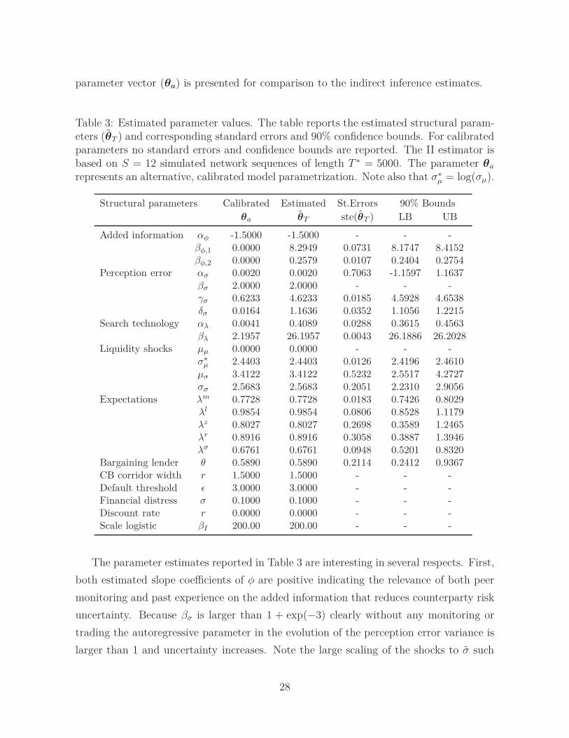
parameter vector (θa) is presented for comparison to the indirect inference estimates.

Table 3: Estimated parameter values. The table reports the estimated structural param-eters (θT ) and corresponding standard errors and 90% confidence bounds. For calibratedparameters no standard errors and confidence bounds are reported. The II estimator isbased on S = 12 simulated network sequences of length T ∗ = 5000. The parameter θa

represents an alternative, calibrated model parametrization. Note also that σ∗µ = log(σµ).

Structural parameters Calibrated Estimated St.Errors 90% Bounds

θa θT ste(θT ) LB UB

Added information αφ -1.5000 -1.5000 - - -βφ,1 0.0000 8.2949 0.0731 8.1747 8.4152βφ,2 0.0000 0.2579 0.0107 0.2404 0.2754

Perception error ασ 0.0020 0.0020 0.7063 -1.1597 1.1637βσ 2.0000 2.0000 - - -γσ 0.6233 4.6233 0.0185 4.5928 4.6538δσ 0.0164 1.1636 0.0352 1.1056 1.2215

Search technology αλ 0.0041 0.4089 0.0288 0.3615 0.4563βλ 2.1957 26.1957 0.0043 26.1886 26.2028

Liquidity shocks µµ 0.0000 0.0000 - - -σ∗

µ 2.4403 2.4403 0.0126 2.4196 2.4610

µσ 3.4122 3.4122 0.5232 2.5517 4.2727σσ 2.5683 2.5683 0.2051 2.2310 2.9056

Expectations λm 0.7728 0.7728 0.0183 0.7426 0.8029λl 0.9854 0.9854 0.0806 0.8528 1.1179λz 0.8027 0.8027 0.2698 0.3589 1.2465λr 0.8916 0.8916 0.3058 0.3887 1.3946λσ 0.6761 0.6761 0.0948 0.5201 0.8320

Bargaining lender θ 0.5890 0.5890 0.2114 0.2412 0.9367CB corridor width r 1.5000 1.5000 - - -Default threshold ǫ 3.0000 3.0000 - - -Financial distress σ 0.1000 0.1000 - - -Discount rate r 0.0000 0.0000 - - -Scale logistic βI 200.00 200.00 - - -

The parameter estimates reported in Table 3 are interesting in several respects. First,

both estimated slope coefficients of φ are positive indicating the relevance of both peer

monitoring and past experience on the added information that reduces counterparty risk

uncertainty. Because βσ is larger than 1 + exp(−3) clearly without any monitoring or

trading the autoregressive parameter in the evolution of the perception error variance is

larger than 1 and uncertainty increases. Note the large scaling of the shocks to σ such

28

that uncertainty is continuously pushed upwards, leading to prohibitively large perceived

probabilities of default that prevent interbank lending in the absence of any trading or

monitoring.

Second, the positive estimate for αλ and βλ shows that counterparty search is a

crucial feature in the formation of interbank networks. It also highlights the effect of

expected profitability and counterparty selection. In particular, the positive estimate for

βλ suggests that links are not formed at random but are strongly influenced by banks’

search towards preferred counterparties. In this respect, the positive point estimate for

the expectation parameter of available interest rates, λr, and available loan volumes,

λz, indicate persistent expectations about credit conditions. Similarly the values of λl

and λm indicate a relatively strong persistence in the expectations of monitoring and

the expectation of being contacted by a specific borrower. These persistent expectation

eventually contribute to the high persistence of the simulated interbank network.

Third, the estimated values of the central liquidity distribution that parameterizes

bank heterogeneity in liquidity shocks point towards considerably different variances in

liquidity shocks. The estimated log normal distribution implies that there are few banks

with very large liquidity shock variances that are very active players in the market.

Moreover the notion that some banks are structural liquidity providers or supplier is

supported by the positive estimate of the variance parameter of the mean. These findings

are in line with previous empirical results, see Furfine (1999) and the core-periphery

structure found by Craig and von Peter (2010).

Table 4: Coefficients of linear policy rule for optimal monitoring

Variable σi,j,t Etσi,j,t+1 Etmi,j,t+1 Etλi,j,t+1 Etζi,j,t+1

Coefficient 0.0431 -0.0223 -0.0165 0.0541 0.0479

In Table 4 we report the coefficients of the linear policy rule for the optimal monitoring

levels as implied by the estimated parameters, expressed in deviations from their mean

steady-state values. It is particular noteworthy that the optimal monitoring level towards

a particular bank depends positively on the expected probability of being approached by

this bank to borrow funds during future trading sessions. Indeed this positive coefficient

and the significantly positive effect of search on link formation creates the interrelation

between monitoring and search as the source of interbank relationship lending. More-

over note that the current state of uncertainty positively affects monitoring during this

29

period, higher expected future uncertainty however reduces these efforts. Also notice the

positive coefficient of the amount of granted loans. Hence, banks prefer to monitor those

counterparties where they expect larger volumes as the surplus that can be generated

by reducing credit risk uncertainty is larger. This implies that banks with on average

opposite liquidity shocks will monitor each other more closely as they will on average

exchange funds of larger quantity. The negative coefficient of expected future monitor-

ing leads to the usual inter-temporal smoothing of expenditures that is well known from

dynamic economic modeling.

Table 5: Testing economic hypotheses

Economic hypothesis H0 θ t-stat Decision1

Monitoring has no effect on information βφ,1 = 0 8.2949 113.47 rejectSearch has no effect on link probability βλ = 0 26.1957 6092.02 rejectNo liquidity shock heterogeneity in mean σ∗

µ = 0 2.4403 193.67 rejectNo liquidity shock heterogeneity in variance σσ = 0 2.5683 12.52 reject1 Decisions are based on 5% significance level

Using the estimated structural model where parameters are associated to clear eco-

nomic concepts, we can test policy-relevant economic theories about the interbank mar-

ket. Table 5 provides a summary of hypotheses about monitoring, search and bank

heterogeneity, along with the respective test statistics and test results. Based on a 5%

significance level we can reject (i) the hypothesis that monitoring has no effects on the

added information, and (ii) the hypothesis that link formation does not depend on banks’

search effort. Thus the data provides evidence of the importance of search and moni-

toring as two key driving forces in the formation of interbank networks. In particular,

the results empirically support the ECB’s view that peer monitoring of counterparty risk

is part of unsecured interbank lending and thereby may justify a decentralized market

solution. Similarly, the result that search has a significant impact on link formation high-

lights the non-random nature of interbank relationships as banks choose those trading

partners that offer them best credit conditions. Furthermore, we can reject the hypothe-

sis that banks have homogeneous liquidity shocks, in both the mean and the variance of

the liquidity distribution. Thus the structure of liquidity shocks in the banking system is

an important reason for the observed interbank network structure and bilateral lending

relations.

30

We next analyze the model fit and auxiliary statistics. Table 6 shows how the esti-

mated structural parameter vector θT produces an accurate description of the data when

compared to the alternative calibrated parameter vector θa stated in Table 3 where

monitoring has no role on information and search has a relatively less important role.

Table 6: Auxiliary statistics. The table reports the values of the observed auxiliarystatistics βT used in the indirect inference estimation along with the HAC robust standarderrors. The simulated average of the auxiliary statistics βT S is shown for the estimatedparameter vector and the alternative calibration. The observed statistics are computedon a sample of daily frequency from 1 February 2008 to 30 April 2011 of size T = 810.

Observed Simulated

Auxiliary statistic βT ste(βT ) βT S(θa) βT S(θT )

Density (mean) 0.0212 0.0026 0.3517 0.0234Reciprocity (mean) 0.0819 0.0028 0.3248 0.3807Stability (mean) 0.9818 0.0025 0.6343 0.9777Std outdegree (mean) 1.8406 0.0917 7.9152 1.7613Std indegree (mean) 1.6001 0.0994 7.4772 1.7500Avg clustering (mean) 0.0308 0.0027 0.3978 0.0887Std clustering (mean) 0.0880 0.0079 0.0321 0.2061Corr(ri,j,t, lrw

i,j,t−1) (mean) -0.0716 0.0112 -0.0001 -0.0726

Corr(li,j,t, lrwi,j,t−1) (mean) 0.6439 0.0106 0.3542 0.5404

Corr(li,j,t, LPIrwi,j,t−1) (mean) 0.4085 0.0085 0.2093 0.1520

Corr(li,j,t, BPIrwi,j,t−1) (mean) 0.4379 0.0090 0.2318 0.1480

Avg log volume (mean) 4.1173 0.0516 2.8292 4.3683Std log volume (mean) 1.6896 0.0200 1.2778 2.0391Avg interest rates (mean) 0.2860 0.1330 1.1276 1.1822Std interest rates (mean) 0.1066 0.0141 0.0013 0.0635Skew interest rates (mean) 0.6978 0.5295 1.8315 1.8091Density (std) 0.0068 0.0004 0.0099 0.0025Corr(density,stability) -0.7981 0.0275 -0.1644 -0.6239

Objective function value 33.5964 1.2390

Euclidean norm ‖βT − βT S‖ 8.7336 1.5973

Sup norm ‖βT − βT S‖∞ 6.0747 1.1113

First note the remarkable improvement in model fit compared to the calibrated exam-

ple, brought about by the indirect inference estimation, as judged by (i) the value of the

(log) criterion function that is about 27 times smaller for the estimated model, and (ii)

the comparison between auxiliary statistics obtained from observed, data simulated at

the calibrated parameter, and data simulated at the estimated parameters. For instance,

31

both the Euclidean norm and the sup norm of the difference between observed and sim-

ulated auxiliary statistics are more than 5 times larger under the calibration without

monitoring.

A closer look at individual auxiliary statistics reveals several interesting features of

the estimated model. First, it is important to highlight the significant improvement in

the fit of the density compared to the calibrated example. In fact the estimated model

matches very well the sparsity of the Dutch interbank network with a density of 0.02

very close to the observed one. Likewise, the present structural model provides a very

accurate description of the high stability of the network and the standard deviations of

the degree distributions. Similarly the average clustering coefficient is improved consid-

erably compared to the calibrated model and matches the data rather well. Hence the

proposed structural economic model is able to generate a lending structure very simi-

lar to the observed one, that is sparse and highly persistence. Both characteristics can

be attributed to the structure of liquidity shocks across banks and asymmetric infor-

mation problems about counterparty risk and search frictions. Indeed, the calibrated

parameter θa parametrized a setting where counterparty risk uncertainty is lower and is

more equally distributed in the cross-section, and loans with different counterparties are

possible without monitoring efforts or past trading experience.

Second, and key to our analysis, the estimated structural model is able to generate

patterns of relationship lending where banks repeatedly interact with each other and

trade at lower interest rates. In particular, the model very accurately matches the ob-

served correlation of interest rates and past trading of -0.072. As reported in Table 4

monitoring efforts positively depend on the expectation about being approached by a

specific borrower. Once a contact between two banks is established, banks positively

adjust their expectation and increase monitoring. This has dampening effects on the

bilateral interest rate level and thereby further attracts the borrower leading to yet in-

creased expectations about a contact. The role of counterparty selection and monitoring

as crucial agents behind the observed dynamic structure of the interbank market is also

confirmed by comparing the fit of the auxiliary statistics simulated under the calibrated

parameter with those of the estimated parameter. We see that the correlation between

past trading and current interest rate increases by a factor of 700 under the estimated

parameter. Also note the positive correlation of 0.54 between past and current bilateral

lending activity, that measures the stability of bilateral lending relationships.

32

Finally, we note also that the model does a poorer job in explaining the observed

average interest rate level. This partly reflects the fact that the model abstracts from

time-varying bank specific outside options for lending and borrowing that are associated

to massive central bank interventions during the financial crisis, in particular after the

Lehman failure. Further, the skewness of the cross-sectional interest rate distribution is

over-estimated and there are too many reciprocal links compared to the observed net-

work. Note also that the model abstracts from any bank heterogeneity beyond differences

in liquidity shocks, in particular differences in balance sheet strength or heterogeneous

outside options.

4 Model Analysis

One of the most appealing features of structural models is the possibility to answer mean-

ingful economic questions and derive relevant policy implications. As we shall now see,

the estimated structural model described above can be used not only to extract relevant

information, but also, as an interesting testing ground for different policies affecting the

interbank lending market. Here we focus on assessing the role of private information,

gathered through monitoring and repeated interaction, in reducing asymmetric infor-

mation problems about counterparty risk and fostering the efficiency of the interbank

market.

4.1 Simulated Paths

Figure 2 below shows a simulated path covering roughly 4 weeks of operations in the in-

terbank market under the estimated structural parameters. In particular, this figure plots

the paths of daily mean log traded volume and daily mean density, stability, reciprocity,

mean monitoring, mean search, perceived error variance (PEV) and link probabilities.

Figure 2 shows also the actual network connections established at three different moments

of time labeled T1, T2 and T3.

The top graph in Figure 2 conveniently shows how daily network density (solid line)

and daily mean log traded volumes (dashed line) are negatively related over time. This

negative relation is justified by the fact that periods of low density are characterized by

the inactivity of smaller banks in the interbank market. The banks that remain active are

large banks whose trade volume is typically large, and hence, average trade volumes rise

33

T1 T2 T3

0.02

0.025

Den

sity

T1 T2 T34

4.5

5

5.5

Vol

ume

T1 T2 T3

0.97

0.98

Sta

bilit

y

T1 T2 T30.3

0.4

0.5

0.6

Rec

ipro

city

T1 T2 T3636

636.5

637

637.5

638

638.5

639

Mon

itorin

g

T1 T2 T31.4

1.42

1.44

1.46

1.48

1.5

1.52

PE

V

T1 T2 T3220

225

230

235

Sea

rch

T1 T2 T30.22

0.225

0.23

0.235

Pro

babi

lity

Figure 2: Simulated 5-week interbank network path and network plots at given momentsof time T1, T2 and T3. Larger nodes reflect larger banks as measured by total lendingand borrowing volume. Left axes correspond to solid lines, right axis to dashed lines.Mean volumes of granted loans are reported in log million euro, mean monitoring andsearch expenditures in thousands of euro.

in crisis periods. From a causal perspective, a larger volume of trade in a given period

will make banks update positively their expectations about future traded volumes, and

34

consequently update positively their expectation on future profit opportunities. This, in

turn, will give an incentive to increase monitoring and search which leads ultimately to

a higher number of trades and higher network density. However, this causal relation is

played out over a number of days and several new shocks will occur in the meanwhile.

As a result, at a daily frequency, the negative contemporaneous relation between density

and average traded volumes remains.

The network plots in Figure 2 are essentially ‘snapshots’ of the network connections

on the days marked T1, T2 and T3. These plots show how the large banks (as measured

by total lending trading), identified here by the larger nodes, are more active on average

(i.e. have more connections with other banks). These banks have more to gain from

interbank market operations and hence monitor and search more. On the contrary, the

smaller banks, depicted in the periphery with smaller nodes, will participate in the market

only sporadically. This is especially true in periods of low activity like T2 when only the

larger banks remain active.

Figure 2 shows also how daily stability (solid line) and daily reciprocity (dashed line)

are positively correlated. This relation is justified by the fact that both stability and

reciprocity are negatively correlated with density, see also the observed and simulated

auxiliary statistics. This negative relation emerges essentially once again because periods

of low density are characterized by the inactivity of smaller banks while the large banks

remain active. Since larger banks tend to create more stable and reciprocal relations

(where they act as both lenders and borrowers), the stability and reciprocity rises. In

essence, in periods of low activity in the interbank market like T2, where only the large

banks with very strong and reciprocal relationships are active, the daily stability and

reciprocity is large. On the contrary, in periods of high activity like T3, smaller banks

that infrequently access the market as either lenders or borrowers become active and

hence the network stability and reciprocity becomes low.

Finally, Figure 2 documents also how monitoring and search (solid lines) and the

perception error variance (PEV) and the link probability (dashed lines) evolve over time.

Inspection of the plotted path for monitoring and PEV reveals that PEV plays a major

role in determining the optimal monitoring decision. The role of PEV on monitoring

decisions is described by the derived Euler equation for monitoring. It is also clear

from the graphs how both monitoring and search are positively related to variations in

density. Indeed, the rise in density influences positively the expected profitability of

35

the interbank market and hence leads to increase in search and monitoring. In turn,

the rise in search and monitoring causes an increase in trade intensity that feeds back

into the system. Similarly, a fall in trade density can have prolonged effects due to this

feedback mechanism. Ultimately, this can lead to a halt in the market. This is clear if

one considers, for example, the decline in density monitoring and search from T1 to T2

and the rise in all three variables until T3.

The events described here are short lived and occur at a high frequency. However,

as we shall see below, depending on the action of central bank authorities, reactions of

a much larger magnitude occurring at a much lower frequency can essentially bring the

interbank market into a halt for extended periods of time.

4.2 Network Uncertainty:

Unconditional Network Properties and

Optimal Search and Monitoring

Figure 3 characterizes the simulated network by describing the distribution of mean den-

sities, interest rates and traded volumes of the top 50 banks operating in the Netherlands

over various possible network structures. In particular, these figures were obtained by

first drawing the bank properties (as described by the parameters µµ, σµ, µσ and σσ) and

then calculating the unconditional mean of densities, interest and volumes both over all

banks and over T = 150 time periods. This procedure was then repeated in a Monte

Carlo setting with 500 replications. Hence, the uncertainty in Figure 3 reflects essen-

tially the uncertainty about the exact network structure as described by the unobserved

liquidity shock distribution.

Figure 3 shows that mean log traded volumes can vary considerably depending on

the network structure. In particular, the inter-quartile includes the observed average

log volume of 4.12 reported in Table 6 but ranges from slightly below 2.5 to above 6.0,

depending on the precise structure of the network. Furthermore, the relative symmetry of

mean log volumes reveals that traded volumes in levels are highly skewed across networks.

This result is justified by the fact that the mean traded volumes depend considerably

on the presence of large complementary banks whose shocks are large in magnitude and

negatively correlated. The presence of two large banks with large liquidity shocks that

feature, on average, liquidity shocks with opposite signs will foster a very efficient usage

36

2.5

3

3.5

4

4.5

5

5.5

6

1

Mean Volumes

1.178

1.18

1.182

1.184

1.186

1.188

1

Mean Interest

0.005

0.01

0.015

0.02

0.025

0.03

0.035

0.04

1

Mean Density

Figure 3: Box plot featuring, median (red line), inter-quantile range (box) and outlierbound (whiskers) of mean log volume, mean interest rate, and mean density with ap-proximately 99% coverage; see McGill et at. (1978).

of the interbank market to smooth shocks as these banks will monitor each other closely

and obtain very favorable interest rates.

Figure 3 also shows that the mean density of the network, which characterizes the

average number of interbank market operations per day, depends strongly on the network

structure. Once again, the inter-quantile range includes the observed density of 0.0212

reported in Table 6 and the large variance is justified by the fact that interbank market

trade is intensified when banks complement each other well and build relations over

time. The interbank market trade is appealing when banks monitor each other and

hence obtain favorable interest rates (relative to the central bank bounds). However,

intense monitoring will only occur when the banks expect significant profit opportunities

in the interbank market. These profit opportunities increase with the size of the liquidity

shocks and the possibility of finding partners facing a symmetric liquidity restriction. As

such, monitoring will be increased in networks featuring banks that face large and/or

symmetric liquidity shocks.

Contrary to the density and volume, Figure 3 shows that the unconditional mean of

interest rates of granted loans is rather stable across different networks. This means that,

for given central bank bounds, different networks will produce largely different outcomes

in terms of mean trade intensity and mean volume, but very similar outcomes in terms

of mean interest rates. In essence, the decision to trade or not is very sensitive to the

37

characteristics of the partners, but the conditions under which trade occurs do on average

not vary much across different network structures.

630

635

640

645

1

Mean Monitoring

15

20

25

30

35

1

Stdev Monitoring

100

150

200

250

300

1

Mean Search

100

150

200

250

300

350

1

Stdev Search

Figure 4: Box plot featuring, median (red line), inter-quantile range (box) and outlierbound (whiskers) of mean and standard deviation of monitoring and search with approx-imately 99% coverage; see McGill et at. (1978).

Figure 4 shows the implied optimal mean and standard deviation in search and mon-

itoring expenditures (annualized expenditures per bank, in thousands of euro) of the top

50 banks operating in the interbank market. As expected, the mean monitoring value is

highly skewed and varies considerably across network structures. Both the large skew-

ness and large variance are in accordance with the analysis made above that argued how

different network structures led to different monitoring efforts, and ultimately, to differ-

ent trade intensities and lending volumes in the interbank market. The same type of

argument is valid for the wide variation in search effort that doubles within the 99% con-

fidence bound. Indeed, since trade opportunities depend on search (which determines the

probability of an open link), the large variation in search is consistent with the observed

large variation in density across network structures. Moreover, our model formulation

allows a boundary solution with zero search expenditures.

Economically, the estimated median of monitoring expenditure is about 635 thousand

euro per bank (annualized), the median of search expenditures about 240 thousand euro.

Note that these figures are for the average bank in the Dutch market, and they are

higher for more active banks. While our model indicates that the cross-sectional standard

deviation of monitoring is relatively low, the cross-sectional standard deviation of search

38

expenditures is considerably larger. An observation that is also driven by the fact that our

model allows a boundary solution with zero search expenditures. This leads, depending

on the network configurations, to the large variance in search.

4.3 Central Bank Policy Analysis:

The Interest Corridor Width Multiplier

Finally, we analyze how changes in the width of the central bank’s interest corridor affect

the market by changing the outside options for lending and borrowing. In particular,

we show how even a small change in the interest bounds can have a strong effect on

the overall interbank market activity. Specifically, we show that due to a reduction in

search and monitoring, the decrease in market activity is a multiple of the decrease in the

bounds. In this sense, we uncover a multiplier for the interbank market that is important

for policy makers. This multiplier increases with the level of monitoring and search.

Figure 5 shows how the width of the EBC corridor produces significant changes in the

mean network density. Again, the uncertainty captured by the quantiles in the box plot

is associated to a larger extent to the uncertainty about the precise network structure.

0.02

0.04

0.06

0.08

0.1

0.12

0.14

0.16

0.18

1.5 1.6 1.7 1.8 1.9 2 2.1ECB Corridor Width

Den

sity

Figure 5: Box plot featuring, median (red line), inter-quantile range (box) and outlierbound (whiskers) of mean network density for different ECB corridor sizes. Each boxplot has approximately 99% coverage; see McGill et at. (1978).

39

The most striking feature of Figure 5 is that an increase of roughly 50% in the width

of the ECB’s interest rate corridor (from 1.5 to 2.1) is predicted to produce a 4 fold

increase in the median network density (average number of daily trades) from roughly

2% density to over 8%. Furthermore, at a corridor width of 2%, the lower bound of the

99% confidence interval across all network structures is larger than the upper bound on

the 99% confidence interval across network structures at a corridor width of 1.5%. This

analysis shows that these effects are highly significant and that the ECB corridor width

plays an important role in the intensity of interbank activity.

A second important feature of Figure 5 is that, since the model is nonlinear, the

multiplier value is not constant over the range of ECB corridor widths. In particular,

Figure 5 shows that the multiplier value is decreasing with corridor width. Indeed, a 0.1

unit increase on the bound has a much larger relative effect in density for low corridor

widths compared to large ones.

The presence of this multiplier, as well as its nonlinearity, are both explained by the

role that monitoring and search play in the interbank market. Just like in the usual

Keynesian multiplier, the effects of a change in the width of the ECB bounds can also

be decomposed into (i) an immediate short-run effect, and (ii) a long-run effect that is

created by the multiplier that results from feedback loops between the effect of monitoring

and search on loan outcomes and expectations about credit conditions.

Consider a decrease in the width of the ECB corridor. In the advent of such a shock,

the interbank market will immediately shrink as a fraction of lending and borrowing op-

erations are no longer profitable given the new tighter ECB bounds. In this immediate

‘mechanical’ effect, part of the interbank market is simply ‘substituted’ by lending and

borrowing with the central bank authority which now plays a more important role. This

immediate short-run effect is however only a fraction of the total long-run effect. Indeed,

given that the possibilities of trade are now smaller, the expected future profit is dimin-

ished and the incentive to monitor and search partners is reduced. This reduction is

monitoring and search (depicted in Figures 6 and 7) will further reduce the mean density

and mean traded volumes in the interbank market. These, in turn force banks to revise

the expected profitability of monitoring and search efforts, pulling these variables further

down. This ‘negative spiral’ that defines the multiplier will bring the market to a new

level of operation that can be orders of magnitude lower than that observed prior to the

bounds.

40

630

635

640

645

650

655

1.5 1.6 1.7 1.8 1.9 2 2.1ECB Corridor Width

Mon

itorin

g

Figure 6: Box plot featuring, median (red line), inter-quantile range (box) and outlierbound (whiskers) of mean monitoring per bank over alternative ECB interest corridorwidth (annualized and in thousands of euro). Each box plot has approximately 99%coverage; see McGill et at. (1978).

Hence, if the ECB wishes to get tighter control over the traded rates by narrowing the

corridor it has to expect further adverse effects on interbank lending activity triggered by

a reduction of monitoring and search. On the other hand, if the ECB wants to foster an

active decentralized interbank lending market as a means to explore benefits from peer

monitoring it is essential to consider policies that increase the difference between the

standing facilities for depositing and lending funds. Only thereby the interbank market

is profitable enough to encourage intense peer monitoring and search among banks. In

both cases the multiplier effect should be taken into account when considering policy

changes.

5 Conclusion

In this paper we propose a structural micro-founded network model for the unsecured

interbank lending market. We use this model to study asymmetric information problems

about counterparty risk and search frictions, and the interaction of both. Specifically

banks are profit maximizing agents that can engage in costly peer monitoring to mitigate

41

150

200

250

300

350

400

450

1.5 1.6 1.7 1.8 1.9 2 2.1ECB Corridor Width

Sea

rch

Figure 7: Box plot featuring, median (red line), inter-quantile range (box) and outlierbound (whiskers) of mean search per bank over alternative ECB interest corridor width(annualized and in thousands of euro). Each box plot has approximately 99% coverage;see McGill et at. (1978).

the counterparty risk uncertainty and search for preferred trading opportunities. We

provided a solution to the banks’ dynamic optimization problems of allocating search and

monitor across potential trading partners. The solution crucially depends on expectations

about future trading opportunities in the network.

In a second part of the econometric analysis we estimate the structural model param-

eters using loan level data at daily frequency collected for the Dutch unsecured overnight

interbank lending market from 2008 to 2011. The parameter vector is estimated with the

method of indirect inference that builds upon a set of auxiliary statistics that capture

the dynamic structure of the observed interbank network. The estimated parameter vec-

tor shows that asymmetric information problems, interacted with monitoring and search

efforts, have significant effects on the network structure and credit conditions. In par-

ticular we find that (i) monitoring has a significant effect on the reduction of credit risk

uncertainty, (ii) monitoring depends positively on the expected future loan probability

and volume, (iii) bilateral lending relationships with increased lending activity and lower

interest rates emerge, similar to those documented in the observed Dutch data, (iv)

the fundamental driving force of trading opportunities are significant differences in the

42

structure of liquidity shocks across banks.

Finally, we use the estimated model to discuss several policy implications. In partic-

ular, we show that in order to foster the trading activity in unsecured interbank markets

and associated benefits from peer monitoring an effective policy measure is to widen the

bounds of the interest corridor. The effects of a wider corridor result from both a direct

effect and a non-linear, indirect multiplier effect triggered through increased monitoring

and search activity among banks.

References

Abbassi, P., Gabrieli, S., and Georg, C.-P. (2013). A network view on money market

freezes. Technical report, mimeo.

Acharya, V. V. and Merrouche, O. (2010). Precautionary hoarding of liquidity and inter-

bank markets: Evidence from the sub-prime crisis. NBER Working Papers 16395,

National Bureau of Economic Research.

Afonso, G., Kovner, A., and Schoar, A. (2011). Stressed, not frozen: The federal funds

market in the financial crisis. Journal of Finance, 66(4):1109–1139.

Afonso, G., Kovner, A., and Schoar, A. (2013). Trading partners in the interbank lending

market. Staff Reports 620, Federal Reserve Bank of New York.

Afonso, G. and Lagos, R. (2012). Trade dynamics in the market for federal funds. Staff

Reports 549, Federal Reserve Bank of New York.

Allen, F. and Gale, D. (2000). Financial contagion. Journal of Political Economy,

108(1):1–33.

Arciero, L., Heijmans, R., Heuver, R., Massarenti, M., Picillo, C., and Vacirca, F. (2013).

How to measure the unsecured money market? the eurosystem’s implementation and

validation using target2 data. DNB Working Papers 369.

Ashcraft, A. B. and Duffie, D. (2007). Systemic illiquidity in the federal funds market.

The American Economic Review, 97(2):221–225.

Babus, A. (2011). Endogenous intermediation in over-the-counter markets. Working

Paper Imperial College London.

43

Bech, M. L. and Atalay, E. (2009). The topology of the federal funds market. Working

Paper Series 986, European Central Bank.

Bougerol, P. (1993). Kalman filtering with random coefficients and contractions. SIAM

Journal on Control and Optimization, 31(4):942–959.

Bräuning, F. and Fecht, F. (2012). Relationship lending in the interbank market and the

price of liquidity. Discussion Papers 22/2012, Deutsche Bundesbank.

Chow, G. C. (1989). Rational versus adaptive expectations in present value models. The

Review of Economics and Statistics, 71(3):376–84.

Chow, G. C. (2011). Usefulness of adaptive and rational expectations in economics.

Working Papers 1334, Princeton University, Department of Economics, Center for

Economic Policy Studies.

Cocco, J. F., Gomes, F. J., and Martins, N. C. (2009). Lending relationships in the

interbank market. Journal of Financial Intermediation, 18:24–48.

Craig, B. R. and von Peter, G. (2010). Interbank tiering and money center banks.

Working Paper 322, Bank for International Settlements.

DeJong, D. N. and Dave, C. (2006). Structural Macroeconometrics. Princeton University

Press.

Diamond, D. W. and Dybvig, P. H. (1983). Bank runs, deposit insurance, and liquidity.

Journal of Political Economy, 91(3):401–19.

Evans, G. W. and Honkapohja, S. (1993). Adaptive forecasts, hysteresis, and endogenous

fluctuations. Economic Review, pages 3–13.

Evans, G. W. and Honkapohja, S. (2001). Learning and expectations in macroeconomics.

Princeton University Press.

Fagiolo, G. (2007). Clustering in complex directed networks. Physics Review E,

76:026107.

Freixas, X. and Holthausen, C. (2005). Interbank market integration under asymmetric

information. The Review of Financial Studies, 18(2):459–490.

44

Furfine, C. H. (1999). The microstructure of the federal funds market. Financial Markets,

Institutions & Instruments, 8:24–44.

Furfine, C. H. (2001). Banks as monitors of other banks: Evidence from the overnight

federal funds market. Journal of Business, 74:33–57.

Gale, D. M. and Kariv, S. (2007). Financial networks. The American Economic Review,

97(2):99–103.

Gourieroux, C., Monfort, A., and Renault, E. (1993). Indirect inference. Journal of

Applied Econometrics, 8(S):S85–118.

Harberger, A. C. (1960). The Demand for Durable Goods. The University of Chicago

Press.

Heer, B. and Maußner, A. (2005). Dynamic general equilibrium modelling. Springer,

Berlin.

Heider, F., Hoerova, M., and Holthausen, C. (2009). Liquidity hoarding and interbank

market spreads: The role of counterparty risk. Working Paper Series 1126, European

Central Bank.

Heijmans, R., Heuver, R., and Walraven, D. (2011). Monitoring the unsecured interbank

money market using target2 data. DNB Working Papers 276, Netherlands Central

Bank, Research Department.

Hommes, C., van der Leij, M., and in ’t Veld, D. (2013). The formation of a core-periphery

networks in over-the-counter markets. Mimeo.

Iori, G., Masi, G. D., Precup, O. V., Gabbi, G., and Caldarelli, G. (2008). A network

analysis of the italian overnight money market. Journal of Economic Dynamics and

Control, 32(1):259 – 278.

Jackson, M. O. (2008). Social and Economic Networks. Princeton University Press,

Princeton, NJ, USA.

Judd, K. L. (1998). Numerical Methods in Economics. The MIT Press.

Mlambo, L. (2012). Adaptive and rational expectations hypotheses: Reviewing the cri-

tiques. The International Journal of Economic Behavior, 2(1):3–15.

45

Rochet, J.-C. and Tirole, J. (1996). Interbank lending and systemic risk. Journal of

Money, Credit and Banking, 28(4):733–762.

Ruge-Murcia, F. J. (2007). Methods to estimate dynamic stochastic general equilibrium

models. Journal of Economic Dynamics and Control, 31(8):2599–2636.

van Lelyveld, I. and in ’t Veld, D. (2012). Finding the core: Network structure in

interbank markets. Technical report, De Nederlandsche Bank Working Paper No. 348.

Weisbuch, G., Kirman, A., and Herreiner, D. (2000). Market organisation and trading

relationships. The Economic Journal, pages 411–436.

White, H. (2001). Asymptotic Theory for Econometricians: Revised Edition . Academic

Press.

A Derivatives in FOC

In the first-order conditions that characterize any interior solution with positive mon-

itoring and search expenditures, we have∂πi,j,t

∂σ2i,j,t

=∂Ri,j,t

∂σ2i,j,t

yi,j,t + Ri,j,t∂yi,j,t

∂σ2i,j,t

and∂πi,j,t

∂si,j,t=

(r − rj,i,t)∂yj,i,t

∂si,j,t. These derivatives can further be unfolded by the chain rule and the

following partial derivatives

∂φi,j,t

∂mi,j,t

= βφ,∂ξi,j,t

∂φi,j,t

=−γσσ2

i,j,t exp(βσφi,j,t)βσ

(1 + exp(βσφi,j,t))2,

∂Pi,j,t

∂σ2i,j,t

=ǫ2

(σ2j,t + σ2

i,j,t + ǫ2)2

∂ri,j,t

∂σ2i,j,t

= 0.5/ǫ2,∂Ri,j,t

∂σ2i,j,t

= −∂Pi,j,t

∂σ2i,j,t

+∂1 − Pi,j,t

∂σ2i,j,t

ri,j,t + (1 − Pi,j,t)∂ri,j,t

∂σ2i,j,t

∂yi,j,t

∂σ2i,j,t

= C ′i,j,t

−βI exp(−βI(ri,j,t − Pi,j,t

1−Pi,j,t))

1 + exp(−βI(ri,j,t − Pi,j,t

1−Pi,j,t))

·

(

∂ri,j,t

∂σ2i,j,t

−∂Pi,j,t

∂σ2i,j,t

(1 − Pi,j,t)−2

)

+βI exp(−βI(r − ri,j,t))

1 + exp(−βI(r − ri,j,t))(−

∂ri,j,t

∂σ2i,j,t

)

Ii,j,t,

∂yj,i,t

∂si,j,t

= C ′′i,j,t

βλ exp(−βλ(si,j,t − αλ))

(1 + exp(−βλ(si,j,t − αλ)))2

where C ′i,j,t := ηi,j,tζi,j,t does not depend on monitoring and C ′′

i,j,t := Ui,j,tIi,j,tζi,j,t does

not depend on the search efforts si,j,t.

46

B Network Auxiliary Statistics

In this section we provide formulas for the non-standard auxiliary statistics that charac-

terize specifically the network structure of the interbank lending market.

densityt =1

N(N − 1)

∑

i,j

li,j,t, reciprocityt =

∑

i,j li,j,tlj,i,t∑

i,j li,j,t

,

stabilityt =

∑

i,j (li,j,tli,j,t−1 + (1 − li,j,t)(1 − li,j,t−1))

N(N − 1).

The interbank network is also characterized by its degree distribution. The degree cen-

trality of a bank counts the number of different trading partners. For directed networks

the out- and in-degree of node i are given by

douti,t =

∑

j

li,j,t and dini,t =

∑

j

lj,i,t.

Instead of considering all 2N variables individually, we consider the mean, variance and

skewness of the out-degree distribution. Note that the mean of degree distribution is

proportional to the density.

The (local) clustering coefficient of node i in a binary unweighted network is given by

ci,t =1/2

∑

j

∑

h(li,j,t + lj,i,t)(li,h,t + lh,i,t)(lj,h,t + lh,j,t)

dtoti,t (dtot

i,t − 1) − 2d↔i,t

,

where dtoti,t = din

i,t + douti,t is the total degree and d↔

i,t =∑

j 6=i li,j,tlj,i,t, see Fagiolo (2007)

for details. We again maintain consider the mean and standard deviation of the local

clustering coefficients.

Second, we compute simple bilateral local network statistics that measure the inten-

sity of a bilateral trading relationship based on a rolling window of size Trw. As a simple

measure of bilateral relationships, we compute the number of loans given from bank i to

bank j during periods t′ = {t − Trw + 1, ..., t} and denote this variable by

lrwi,j,t =

∑

t′

li,j,t′,

where the sum runs over t′ = {t − Trw + 1, ..., t}. Further, for any bank pair we compute

47

the lender and borrower preference index during the rolling window

LP Ii,j,t =yi,j,t′

∑

j,t′ yi,j,t′

and BP Ii,j,t =yi,j,t′

∑

i,t′ yi,j,t′

that measure the relative importance of banks forming a pair in terms of portfolio con-

centration.

48

C Summary statistics of the data

Table 7: Descriptive Statistics of Dutch Interbank Network: The table shows momentstatistics for different sequences of network statistics and cross-sectional correlations thatcharacterize the sequence of observed Dutch unsecured interbank lending networks. Thestatistics are computed on a sample of daily frequency from 1 February 2008 to 30 April2011.

Statistic Mean Std Autocorr Skew Kurtosis

Density 0.0212 0.0068 0.8174 0.8667 3.1983Reciprocity 0.0819 0.0495 0.2573 0.2903 2.8022Stability 0.9818 0.0065 0.8309 -0.8590 3.0503Mean-out-/indegree 1.0380 0.3323 0.8174 0.8667 3.1983Std-outdegree 1.8406 0.4418 0.6882 0.0553 2.4326Skew-outdegree 2.8821 1.0346 0.7035 0.6074 2.4572Mean-indegree 1.0380 0.3323 0.8174 0.8667 3.1983Std-indegree 1.6001 0.4140 0.6880 0.6997 3.4529Skew-indegree 2.4030 0.8787 0.6576 0.6714 2.7434Outdegree-corr 0.0000 0.0000 -0.0225 -0.2675 5.6217Indegree-corr 0.0000 0.0000 -0.0604 0.1348 4.6186Mean-clustering 0.0308 0.0225 0.4149 0.7900 3.2473Std-clustering 0.0880 0.0490 0.3587 0.1561 2.7280Skew-clustering 3.7367 1.5454 0.1213 -0.2213 3.1281Avg log-volume 4.1173 0.2818 0.4926 -0.2820 2.8220Std log-volume 1.6896 0.1685 0.3623 0.1541 3.4546Skew log-volume -0.3563 0.2818 0.2970 -0.0669 3.2151Avg rate 0.2860 0.3741 0.9655 1.1044 2.6965Std rate 0.1066 0.0632 0.7865 1.6668 6.8848Skew rate 0.6978 1.6399 0.5492 0.6832 2.9469Corr(r,lrw) -0.0716 0.1573 0.4066 0.0817 2.8539Corr(l,lrw) 0.6439 0.0755 0.4287 -0.7653 4.2833Corr(l,LPIrw) 0.4085 0.0749 0.4365 -0.1585 3.8179Corr(l,BPIrw) 0.4379 0.0730 0.4604 -0.3398 3.4158

49

D Indirect Inference Weights

Following Gourieroux et al. (1993), we adopt a quadratic objective function for indirect

inference estimation with diagonal weight matrix based on the optimal weighing matrix

that is obtained as the inverse of the covariance matrix of the auxiliary statistics. In

particular, we set the criterion function to

θT := arg maxθ∈Θ

[

βT −1

S

S∑

s=1

βT,s(θ)]

WT

[

βT −1

S

S∑

s=1

βT,s(θ)]′

,

but we use a weight matrix WT that differs from the optimal for several reasons. First, the

inverse of the covariance matrix is only optimal under an axiom of correct specification.

Moreover, even under correct specification the (asymptotically) optimal weighing matrix

can lead to larger variance of the estimator in finite samples. Second, for economic

theoretic reasons, there are a number of auxiliary statistics that we wish to approximate

better than others.

As such we adopt a matrix WT corresponding to a tanh transformation of the the

diagonal of the inverse of the covariance matrix of the auxiliary statistics. Further

the weight of the density and corr(li,j,t, lrwi,j,t−1) is increased by 10 and the weight of

corr(ri,j,t, lrwi,j,t−1) is increased by 500 as we want to match these characteristics partic-

ularly well. For computational reasons we minimize the logarithmic transformation of

the objective function. For each of the S = 12 network paths we burn 1000 periods to

minimize dependence on the initial value. The numerical optimization of the objective

function is done using a grid search algorithm.

50