Contents lists available at ScienceDirect

Economic Modelling

journal homepage: www.elsevier.com/locate/econmod

A dynamic Nelson-Siegel yield curve model with Markov switching☆

Jared Levanta,⁎, Jun Mab

a Regions Bank, Birmingham, AL, USAb Culverhouse College of Commerce & Business Administration, University of Alabama, Tuscaloosa, AL, USA

A R T I C L E I N F O

JEL:C51E43

Keywords:Nelson–Siegel yield curve modelRegime shiftsState-Space modelKalman filterKim algorithm

A B S T R A C T

This paper proposes a model to better capture persistent regime changes in the interest rates of the US termstructure. While the previous literature on this matter proposes that regime changes in the term structure aredue to persistent changes in the conditional mean and volatility of interest rates we find that changes in a singleparameter that determines the factor loadings of the model better captures regime changes. We show that thismodel gives superior in-sample forecasting performance as compared to a baseline model and a volatility-switching model. In general, we find compelling evidence that the extracted factors from our term structuremodels are closely related with various economic variables. Furthermore, we investigate and find evidence thatthe effects of macroeconomic phenomena such as monetary policy, inflation expectations, and real economicactivity differ according to the particular regime realized for the term structure. In particular, we identify theperiods where monetary policy appears to have a greater effect on the yield curve, and the periods whereinflation expectations seem to have a greater effect in yield determination. We also find convincing evidence of arelationship between the regimes estimated by the various switching models with economic activity andmonetary policy.

1. Introduction

The yield curve often contains useful information about realeconomic activity and inflation. For example, the level factor (thelong-term yield-to-maturity) is often argued to be closely related withinflation expectations, while the steepness or the slope factor (the long-term yield-to-maturity minus the short-term yield-to-maturity) hasbeen shown to vary with the business cycles and is heavily influencedby monetary policy (see Evans and Marshall (1998), and Wu (2002)).The most recent monetary policies, such as Operation Twist conductedby the Federal Reserve Bank in an attempt to lower the long-terminterest rate and raise the short-term rate, directly work on the yieldscurve and serve as a great example of how the yield curve, instead ofjust one single policy rate–federal funds rate–is expected to have asignificant impact on the economy. As such, it is important to correctlymodel the yield curve to understand better its interactions withbusiness cycles, and the monetary policy transmission mechanismthrough its impact on the yield curve.

The interaction of the term structure and the macroeconomy hasbeen investigated by a growing work of empirical literature. Examplesinclude (but are not limited to) Diebold and Li (2006), hereafter DL)

and Diebold et al. (2006), hereafter DRA) who employ a generalizedversion of the Nelson and Siegel (1987), hereafter NS) yield curvemodel. More recently, Christensen et al. (2011) place the NS model in atheoretically consistent arbitrage-free framework. In this paper, we relyon the results of Coroneo et al. (2011) who finds the NS model is closeto being arbitrage-free when applied to the US market, although it doesnot explicitly impose these restrictions.

Another stream of literature has shown the US interest ratedynamics of the term structure to be subject to frequent regimechanges (see Bansal and Zhou (2002)). Although some regime changesare results of obvious changes in monetary policy as in the Volcker eraand obvious changes in business cycle conditions such as the oil supplyshock of the 1970s, there are many other regime changes that are dueto more frequent business cycle fluctuations and often indirectlyobserved changes in the financial markets. Chauvet (1998) introducesregime switching to a dynamic factor model of business cycle fluctua-tions and thus accurately captures asymmetries associated witheconomic expansions and contractions. Startz and Tsang (2010)incorporate Markov regime switching into an trend/cycle unobservedcomponents model of the yield curve to account for regime changes ofthe yield curve. Abdymomunov and Kang (2015) find the differences in

http://dx.doi.org/10.1016/j.econmod.2016.10.003Received 1 June 2016; Received in revised form 15 September 2016; Accepted 9 October 2016

☆We are grateful to James Hamilton, James Morley, seminar participants of the International Association Applied Econometrics 2014 Annual conference, participants of the Societyof Nonlinear Dynamics and Econometrics 2014 Annual symposium, two anonymous referees, and an editor for comments.

⁎ Corresponding author.E-mail addresses: jaredmslevant@gamil.com (J. Levant), jma@cba.ua.edu (J. Ma).

Economic Modelling xx (xxxx) xxxx–xxxx

0264-9993/ © 2016 Elsevier B.V. All rights reserved.Available online xxxx

Please cite this article as: Levant, J.M., Economic Modelling (2016), http://dx.doi.org/10.1016/j.econmod.2016.10.003

the term spread across regimes is explained through the term premiarather than expectations of future short rates. Capturing regimechanges in order to model the dynamic movements of the yield curvemore accurately is becoming a growing source of investigation in theterm structure literature as seen in Xiang and Zhu (2013) and Heviaet al. (2015). In particular, our paper differs from Hevia et al. (2015) ina number of important dimensions. First, Hevia et al. (2015) did notreport the estimation results of the model with Markov-switchingvolatility while we find such a model provides important insights formodeling the yields curve. We also conducted statistical exercises toaccount for the Davies’ nusance parameter issue in efforts to formallytest for the significance of the Markov-switching model relative to thebaseline no-switching model (Section 4.5), which Hevia et al. did notattempt to do. Finally, we document the important connectionsbetween the regime switchings and macroeconomic indicators usinglogit models in Section 4.6. In sum, our work made a number ofimportant contributions that are outside the scope of Hevia et al.(2015).

In this paper, we model the parameter instability in the termstructure and relate the regime switching to economic fundamentals byapplying a Markov-switching component to the factor loading para-meter which controls the influence of the slope and curvature yieldfactors on yields. As mentioned previously, the literature has relatedthe slope factor to monetary policy. Also, it has been shown that thecurvature factor is heavily influenced by monetary policy as well (seeDewachter and Lyrio (2008) and Bekaert et al. (2010)). In the extantliterature, concerning the factor loading parameter, this parameter hasbeen primarily utilized in improving the forecasting ability of the NSmodel (see Svensson (1995)), Christensen et al. (2009), Koopman et al.(2010)). By assuming the factor loading parameter follows a two-stateMarkov-process we are able to improve the forecasting ability of the NSmodel while gaining insight into regime changes of the term structurethrough the macroeconomic fundamental variables, inflation expecta-tions and monetary policy. Recently, Yu and Salyards (2009) and Yuand Zivot (2011) apply a dynamic NS model to modeling corporatebond yields and they find that the optimal factor loading parameter,changes as one goes from modeling investment to speculative gradebonds. Their results corroborate our findings in general.

We contribute to the literature by introducing and thoroughlyevaluating regime-switching factor loadings and regime-switchingvolatility in the dynamic Nelson-Siegel model. In our models, regimesare characterized by a latent Markov switching component—the fourthlatent factor. We apply a Markov switching component to the loadingparameters of the factors as well as the factors’ volatility. Comparisonsbetween the models are made by presenting goodness-of-fit statisticsand AIC/BIC values. We also implement the Likelihood Ratio (LR)tests to investigate if our models are statistically different from thebaseline linear DL model. Although both models are found to bestatistically different from the baseline model, the root mean squareerror (RMSE) analysis shows the model with the loading parameterswitching yields the smallest RMSE across the short, medium, and longmaturity ranges and in terms of overall fit. This model also gives theminimum AIC/BIC values of all models under consideration.

In light of recent discussions about potential interactions betweenthe interest rates factors and the macro-economy, we investigate therelationship between the extracted factors from our DNS models andthe observed macroeconomic variables. We find that our interest ratefactors, which are extracted separately from the macroeconomicvariables, are closely related with the macro-economy. Specifically,we find the level factor is strongly correlated with the inflationexpectation, and the slope factor appears to be counter-cyclical, whichis consistent with the finding by Wu (2002) that the slope factor isrelated with monetary policy. Furthermore, in the regime-switching DLmodel we find that the loading of the slope factor on the yield curve islarger during recessions than expansions. This seems to suggest anasymmetric effect of the monetary policy on the yield curve over

business cycles.This paper is organized as follows. Section 2 describes the baseline

dynamic Nelson-Siegel model and the regime-switching DNS model.Section 3 describes the data. Section 4 presents and discusses theestimation results. Section 5 concludes. Appendices discuss the estima-tion procedure via Kalman filter (KF) and the Kim algorithm (KA).

2. Models and estimation

In this section we introduce the baseline dynamic Nelson-Siegel(DNS) model. The appeal of the DNS model lies in its extension to thetime dimension. We also introduce our regime-switching extensions ofthe DNS models and the estimation technique used.

2.1. The Dynamic Nelson-Siegel Model

The Diebold and Li (2006) factorization of the NS model is given by

⎛⎝⎜

⎞⎠⎟F λy (m)=y (m; , )=L +S 1−e

λm+C 1−e

λm−ett t t t

−λmt

−λm−λm

(1)

where F=(L , S , C )′t t t t is a vector representing level, slope, and curvatureof the yield curve, for given time t , maturity m, and constant λ, thefactor loading parameter. This is the baseline DNS model in ouranalysis.

The shape of the yield curve comes from the factor loadings andtheir respective weights in Ft . From Eq. (1), the factor loadingassociated with Lt is assumed to be unity for all maturities andtherefore influences short, medium, and long-term interest ratesequally. The loading factors for St and Ct depend on both maturityand the loading parameter. For a given t , the slope factor loadingconverges to one as λ ↓ 0 (or m ↓ 0) and converges to zero as λ → ∞ (orm → ∞). The curvature factor loading converges to zero as λ ↓ 0 (orm ↓ 0) and as λ → ∞ (or m → ∞) for a given t .

Since we are interested in the loading parameter's effect on yields,we use the limit analysis above to understand the asymptotic behaviorof the yield curve. The yield curve converges to L S+ as λ ↓ 0 andconverges to L as λ → ∞ for a given t . These limiting values indicatethat without the loading parameter the yield curve is flat and withextreme values for the loading parameter the yield curve would becomeflat. So both “reasonable” values for λ and the level factor areresponsible for the wide range of non-flat yield curve shapes withinan NS framework.

2.2. DNS model estimation

We adopt the DRA state-space framework to model each variant ofthe NS model in this paper. Our measurement equation models thetime-series process of the yields according to the latent factors andtakes the form

⎛

⎝

⎜⎜⎜⎜

⎞

⎠

⎟⎟⎟⎟

⎛

⎝

⎜⎜⎜⎜⎜⎜⎜

⎞

⎠

⎟⎟⎟⎟⎟⎟⎟

⎛

⎝⎜⎜

⎞

⎠⎟⎟

⎛

⎝

⎜⎜⎜⎜

⎞

⎠

⎟⎟⎟⎟

y (m )y (m )

⋮y (m )

=

1 −e

1 −e

⋮ ⋮ ⋮

1 −e

LSC

+

ε (m )ε (m )

⋮ε (m )

t 1

t 2

t N

1 − eλm

1 − eλm

−λm

1 − eλm

1 − eλm

−λm

1 − eλm

1 − eλm

−λm

t

t

t

t 1

t 2

t N

−λm1

1

−λm1

11

−λm2

2

−λm2

22

−λmN

N

−λmN

NN

(2)

or expressed in matrix notation as

y F ε ελ MN t TΛ Σ= ( ) + , ∼ (0, ), =1,…,t t t t ε (3)

with yt representing the N × 1 vector of yields, N × 3 factor loadingmatrix λΛ( ),3 × 1 latent factor vector Ft , and N × 1 yield disturbancevector εt (or so-called measurement errors of the yields). The diagonalstructure of Σε implies that measurement errors across maturities of ytare uncorrelated and is a fairly standard assumption in the literature.The transition equation, which models the time series process of the

J. Levant, J. Ma Economic Modelling xx (xxxx) xxxx–xxxx

2

latent factors, can be expressed by the vector autoregressive process oforder one

⎛

⎝⎜⎜⎜

⎞

⎠⎟⎟⎟

⎛

⎝⎜⎜

⎞

⎠⎟⎟

⎛

⎝

⎜⎜⎜

⎞

⎠

⎟⎟⎟⎛

⎝⎜⎜

⎞

⎠⎟⎟

μμμ

μμμ

ηηη

L −S −C −

=a 0 00 a 00 0 a

L −S −C −

+L

S

C

L

S

C

L

S

C

t

t

t

11

22

33

t−1

t−1

t−1

t

t

t

t

t

t (4)

or expressed in matrix notation as

F I A μ A F I A μ η( −( − ) ) = ( −( − ) ) + ,t t t−1

−1−1 (5)

with 3 × 1 mean vector μ, 3 × 3 coefficient matrix A, and 3 × 1factordisturbance matrix Ση. In this investigation we assume a diagonalcoefficient matrix based on the findings of Diebold et al. (2006) andChristensen, Diebold, and Rudebusch (2011) who show the off-diagonal elements of the A matrix are not statistically relevant tomodeling the term structure. We also assume Ση follows a diagonalstructure implying the factor disturbances are uncorrelated. Once againwe look to Diebold et al. (2006), which finds the off-diagonal elementsof the factor covariance matrix to be marginally significant.Furthermore, they note that when the model is estimated with therestriction that the factor covariance matrix be diagonal, the pointestimates and standard errors of the A matrix are little changed fromwhen the model is estimated with no restriction on Ση.

Since the DNS state space model is linear in latent factors, we areable to use the Kalman (1960) filter to estimate the latent factorsconditional on past and contemporaneous observations of the yields.Appendix A gives a detailed description of the filtering process.

2.3. DNS model with Regime-Switching loading parameter

In sub-Section 2.1 we established that λ and Lt determines theshape of the yield curve. Thus changes in interest rate levels aredetermined by both λ and Lt, given other factors. Realizing that keepingλ fixed across the sample period may be a source of model mis-specification in the literature (see Diebold and Li (2006), Diebold et al.(2006), Xiang and Zhu (2013)), Koopman et al. (2010) treat λ as atime-varying latent factor of the model to be estimated in the samefashion as the latent NS factors of the model.

We model λ as a regime-switching parameter that influencesinterest rate levels according to the realized state. We assume the termstructure follows a two-state regime switching process for computa-tional tractability of our model. Investigating ex-post real interest rates,Garcia and Perron (1996) assume interest rates follow a three-stateregime switching process. And using a reversible jump Markov chainMonte Carlo (RJMCMC) procedure, Xiang and Zhu (2013) estimatetwo distinct regimes for the term structure.

We propose to treat the loading parameterλas a regime switchingparameter solely determined by the realized state, ψt of the yields. Thelatent Markov component ψt is governed by a two-state Markov processand we denote the states simply as 0 or 1 corresponding to the termstructure being in the low or high regime, respectively. The loadingmatrix λΛ( ) in Eq. (3) is replaced by λΛ( )ψt and the resultingmeasurement equation is y F ελΛ= ( ) +t t tψt . Take note that since we arenot including λ in Ft , the observation vector of yields is still linear withrespect to our latent factor vector. The modified state-space frameworkfor the dynamic Nelson-Siegel model for estimation with regime-switching the loading parameter is as follows:

y F ε ε F I A μ AF η ηλ MN t T MN

t T

Λ Σ

Σ

= ( ) + , ∼ (0, ) =1,…, =( − ) + + , ∼

(0, ), =1,…,t ψ t t t ε t t t t

η

−1t

(6)

λ λ ψ λ ψ ψ= (1 − )+ , =0, 1ψ t t t0 1t

These equations written in matrix notation constitute the DynamicNelson-Siegel with Markov-Switching Lambda (DNS-MSL) model.Details of the estimation process can be found in Appendix B.

2.4. The DNS Model with Regime-Switching Factor Volatilities

In most of the empirical literature on term structure modeling, aconstant volatility is assumed in the time-series of interest rates. Likemodeling the DNS model with constant loading parameter, a constantvolatility over time may be a source of model misspecification forestimating the term structure. A few papers investigate time-varyingvolatility in the context of the DNS model. Bianchi et al. (2009) employa VAR augmented with NS factors and macro-factors featuring time-varying coefficients and stochastic volatility. Koopman et al. (2010)estimate yield disturbances according to a GARCH specification tointroduce a time-varying variance.

We modify the DNS model by introducing regime-switchingvolatility to the factor disturbances in the transition equation. Themodified state-space framework for the dynamic Nelson-Siegel modelfor estimation with regime-switching the factor volatilities is as follows:

⎛⎝⎜

⎞⎠⎟

y F ε ε F I A μ AF η ηλ MN t T MN

t T

Λ Σ

Σ

= ( ) + , ∼ (0, ) =1,…, =( − ) + + , ∼

0, , =1,…,

t t t t ε t t ψ t

η

−1 t

ψt (7)

η η ψ η ψ ψ= (1 − )+ , =0, 1ψ t t t0 1t

These equations constitute the Dynamic Nelson-Siegel withMarkov-Switching Volatility (DNS-MSV) model. Details of the estima-tion process can be found in Appendix B.

3. DATA

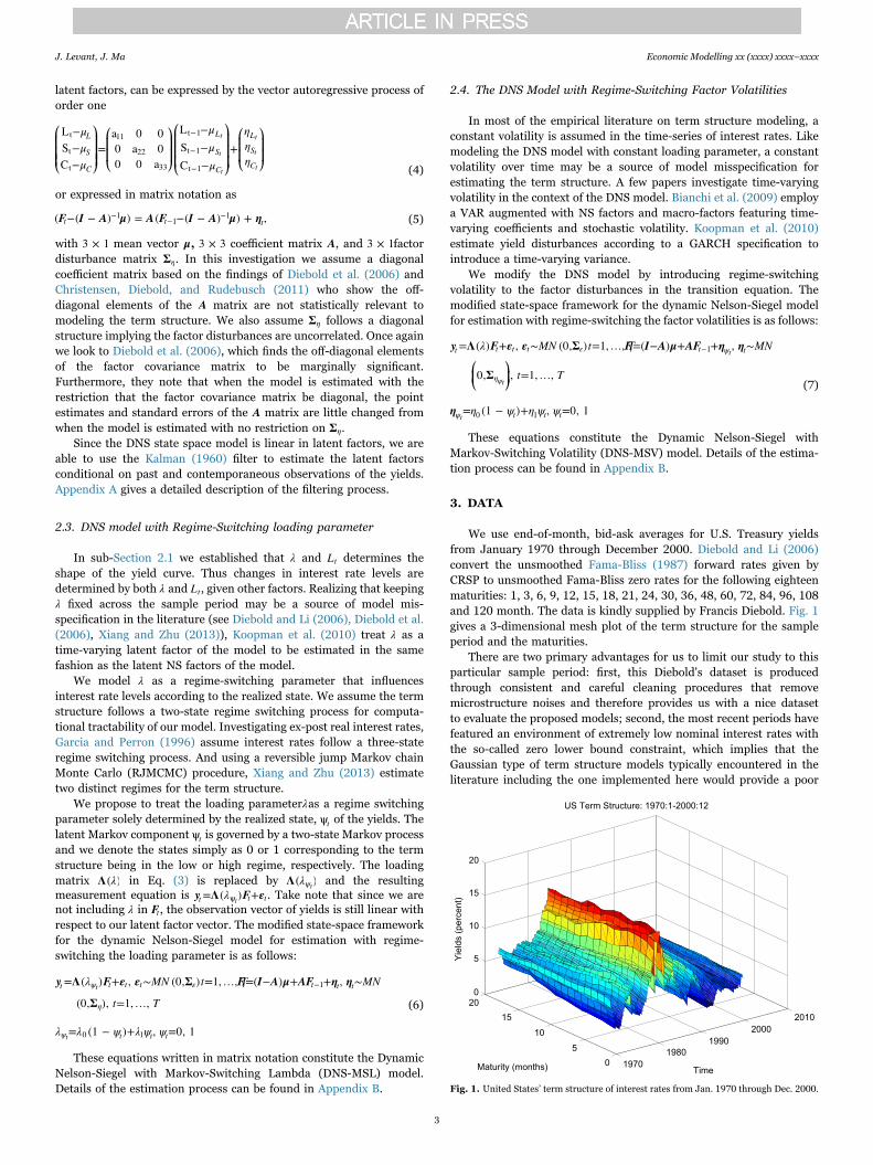
We use end-of-month, bid-ask averages for U.S. Treasury yieldsfrom January 1970 through December 2000. Diebold and Li (2006)convert the unsmoothed Fama-Bliss (1987) forward rates given byCRSP to unsmoothed Fama-Bliss zero rates for the following eighteenmaturities: 1, 3, 6, 9, 12, 15, 18, 21, 24, 30, 36, 48, 60, 72, 84, 96, 108and 120 month. The data is kindly supplied by Francis Diebold. Fig. 1gives a 3-dimensional mesh plot of the term structure for the sampleperiod and the maturities.

There are two primary advantages for us to limit our study to thisparticular sample period: first, this Diebold's dataset is producedthrough consistent and careful cleaning procedures that removemicrostructure noises and therefore provides us with a nice datasetto evaluate the proposed models; second, the most recent periods havefeatured an environment of extremely low nominal interest rates withthe so-called zero lower bound constraint, which implies that theGaussian type of term structure models typically encountered in theliterature including the one implemented here would provide a poor

Fig. 1. United States’ term structure of interest rates from Jan. 1970 through Dec. 2000.

J. Levant, J. Ma Economic Modelling xx (xxxx) xxxx–xxxx

3

approximation and thus calls for separate treatment that we leave forfuture studies.

Table 1 reports the means, standard deviations, and autocorrela-tions across maturities for the yields with maturities of 1, 12, and 30months. The summary statistics show the average yield curve is upwardsloping –a reflection of the risk premium inherent in longer maturities.The volatility is generally decreasing by maturity with the exceptions ofthe one-month being less volatile than the 3, 6, and 9-month bills andthe 8-yr being less volatile than the 9-yr bond.

We also report the statistics for the empirical counterparts for thelevel, slope, and curvature factors. It is worth declaring which conven-tion we adopt in calculating the empirical factors.1 The empirical levelfactor is calculated as an average of the 1, 24, and 120 monthmaturities. The empirical slope factor is the difference between the120 and 1 month maturities. Lastly, the empirical curvature factor istwice the 24 month maturity minus the sum of the 1 and 120 month.

4. Emprical results

In this section we present the model estimation, comparative testresults, and explore a macro-factor linkage with the DNS, DNS-MSL,and DNS-MSV models. Parameter estimates of each model via KF andKA are presented and discussed. We then look at in-sample estimationthrough root mean squared error analysis and information criterioncalculations. We test to see if the Markov-switching models aresignificantly different from the baseline model using a bootstrappedLR test. Finally, we use logit regressions to explore if the estimatedregimes are related to macro-factors for inflation expectations, eco-nomic activity and monetary policy.

4.1. DNS model

The baseline DNS model is estimated with parameter estimatevalues close to those of other DNS parameter estimates in theliterature. The parameter estimates are listed in Table 2.

The estimate for the loading parameter λ is 0.080 with a standard

error of 0.0035 while the estimated λ for Diebold, Rudebusch andAruoba (2006) is 0.077 and 0.078 for Koopman et al. (2010). Using theDiebold and Li's interpretation of λ we are able to ascertain thematurity in which the loading on the curvature factor attains amaximum, henceforth referred to as implied maturities. Recall theloading on the curvature factor (CL) has functional form

CL = 1−eλm

−e .−λm

−λm(8)

Taking the first order condition of CL with respect to the maturity,m, yields

Table 1Descriptive statistics: 1970.1–2000.12.

Maturity Mean Std. dev. Minimum Maximum ρ (1) ρ (12) ρ (30)

1 6.44 2.58 2.69 16.16 0.966 0.692 0.2963 6.75 2.66 2.73 16.02 0.973 0.714 0.3136 6.98 2.66 2.89 16.48 0.974 0.730 0.3509 7.10 2.64 2.98 16.39 0.974 0.738 0.37512 7.20 2.57 3.11 15.82 0.973 0.742 0.35915 7.31 2.52 3.29 16.04 0.974 0.750 0.42318 7.38 2.50 3.48 16.23 0.975 0.757 0.44221 7.44 2.49 3.64 16.18 0.976 0.761 0.45624 7.46 2.44 3.78 15.65 0.976 0.758 0.46530 7.55 2.37 4.04 15.40 0.976 0.768 0.48836 7.63 2.34 4.20 15.77 0.978 0.774 0.50048 7.77 2.28 4.31 15.82 0.978 0.780 0.52460 7.84 2.25 4.35 15.00 0.981 0.794 0.54372 7.96 2.22 4.38 14.98 0.981 0.803 0.55684 7.99 2.18 4.35 14.98 0.981 0.786 0.56096 8.05 2.17 4.43 14.94 0.983 0.812 0.574108 8.08 2.18 4.43 15.02 0.983 0.813 0.580120 8.05 2.14 4.44 14.93 0.983 0.789 0.570

Empirical FactorsLevel 7.32 2.31 4.08 15.26 0.980 0.771 0.466Slope -1.60 1.45 -5.00 3.33 0.910 0.342 -0.104Curvature 0.43 0.84 -1.80 3.93 0.736 0.207 0.124

Note: We define the Level as (y(1)+y(24)+ y(120))/3, the Slope as y(120) – y(1) andCurvature as 2*y(24) – (y(1) + y(120)).

Table 2Parameter Estimates for the DNS, DNS-MSL, and DNS-MSV models.

Parameters DNS DNS-MSL DNS-MSV

a11 0.95 0.99 0.99(0.0178) (0.0045) (0.0054)

a22 0.91 0.98 0.99(0.0256) (0.0150) (0.0094)

a33 0.88 0.79 0.90(0.0569) (0.0322) (0.0244)

μ11 9.22 7.57 6.85

(0.6655) (0.5789) (0.4108)

μ22 -1.50 -1.52 0.83

(0.1858) (0.5368) (0.3913)

μ33 -0.47 0.16 -0.66

(0.0543) (0.2409) (0.4098)

σηL0 0.36 0.33 0.50

(0.0225) (0.0146) (0.0197)

σηS0 0.62 0.61 1.22

(0.0169) (0.0248) (0.0212)

σηC0 0.92 1.03 1.87

(0.0283) (0.0521) (0.0438)

σηL1 – – 0.26

(0.0534)

σηS1 – – 0.33

(0.0686)

σηC1 – – 0.61

(0.1275)

λ0 0.080[22.4] 0.153[11.7] 0.081[22.1]

(0.0035) (0.0022) (0.0017)

λ1 – 0.055[32.6] –

(0.0043)

q – 0.90 0.89p – 0.93 0.97Max. Likelihood Value 9243.6 9481.7 9435.3Number of free parameters (k) 28 31 33AIC -18431.2 -18901.4 -18804.6BIC -18240.6 -18690.4 -18578.0

Standard errors are in parentheses.Implied maturities measured in months are in brackets.We calculate the information criteria according to the formulas θAIC k= −2*ℓ( ) +2*maxand

θBIC k NT= −2*ℓ( ) + * ln ( )max , where N = 18 maturities and T = 371 months.

1 Some authors define empirical level as simply the observed long term maturity,which in our case would be y(120).

J. Levant, J. Ma Economic Modelling xx (xxxx) xxxx–xxxx

4

CL eλ

me emλ

= + − 1− .mλm

λmλm−

−−

2 (9)

Setting this nonlinear equation to zero and solving for m gives thematurity that the curvature loading reaches a maximum. The impliedmaturity of our estimated DNS model is 22.4 months while the impliedmaturity in the DRA paper is 23.3 months.

Our estimated smoothed factors from the DNS model have rela-tively high correlations to the empirical factors as shown in Table 3.

In fact, the smoothed factors of this model give the highestcorrelations for each empirical factor of all the models estimated.Fig. 2 gives a visual of the time-series of each estimated factor plot withthe time-series of the empirical factors.

4.2. DNS-MSL model

We now introduce the first of our two regime switching models–theDNS-MSL model. Comparing the correlations of our estimatedsmoothed factors for this model and their respective empirical factorsfrom Table 3 we find a drop in the correlations across the factors ascompared with the baseline non-switching model. Specifically, thecurvature factor experiences the largest decrease of all the models. This

is further supported with a visual inspection of the third plot of thesmoothed-empirical factor plots of Fig. 3.

There are two causes for this drastic decrease in the correlation ofthe smoothed curvature factor and its empirical counterpart in bothswitching models. First, the empirical factors are calculated under theassumption of no switching in yields. Therefore the factors responsiblefor capturing the switching we propose exists in the term structure –slope and curvature—should experience the largest decreases incorrelation with empirical slope and curvature. Second, and morespecifically for the curvature factor, the literature has shown that thecurvature factor is highly volatile and thus may suffer from weakidentification and therefore its estimation is the most tenuous of all theestimable factors. It is indeed the case that for each model we estimatethe curvature factor has the highest volatility.

Our estimation results from the KF indicate the loading parameter λis subject to a hidden Markov switching component. We estimate λ tobe 0.055 (32.6 months) and 0.153 (11.7 months) for the low and highregimes, respectively. Fig. 4 shows the effect these values have on theslope and curvature factor loadings across maturities.

In the first two plots we see a much faster decay of the slope andcurvature loading factors in the high λ regime than in the low λ regime.This indicates that in the high λ regime the slope and curvature factorloadings (which are directly dependent on λ) influence medium andlong-term maturities less than in the lowλ regime. Yields for mediumand long-term maturities are determined more by long-term inflationexpectations during regimes when λ is relatively high–because thedecay of the slope and curvature factors is greater–and more byeconomic activity and monetary policy when λ is low –because thedecay of the slope and curvature factors is relatively less.

From the third plot in Fig. 4, we see that the slope loading factor isuniformly greater across maturities in the low regime than in the highregime. This shows that the slope factor– proxying for monetarypolicy–contributes more to yield determination over all maturities inthe low λ regime relative to inflation expectations. In the last plot, thecurvature loading factor is greater in the high regime than in the lowregime for the one through 19-month maturities and thereforeinfluences the yields of those maturities more so than in the lowregime. For longer maturities in the high regime, the curvature loading

Table 3Correlations between the empirical and estimated factors.

DNS DNS-MSL DNS-MSV

ρLEMP LEST, 0.8987 0.8598 0.8768

(0.010) (0.013) (0.012)

ρSEMP SEST, 0.9558 0.9064 0.9061

(0.004) (0.009) (0.009)

ρCEMP CEST, 0.8749 0.6374 0.7429

(0.012) (0.028) (0.023)

Note: ρxy is the correlation coefficient between quantities x and y, LEMP is the empirical

level factor, LEST is the estimated level factor, SEMP is the empirical slope factor, SEST is

the estimated slope factor, CEMP is the empirical curvature factor, and CEST is the

estimated curvature factor. Standard errors are in parentheses.

Fig. 2. Smoothed factor plots for the DNS model.

J. Levant, J. Ma Economic Modelling xx (xxxx) xxxx–xxxx

5

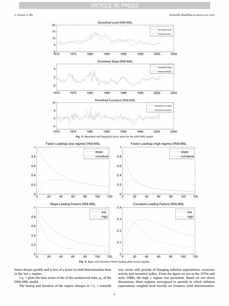
factor decays quickly and is less of a factor in yield determination thanin the low λ regime.

Fig. 5 plots the time series of the of the unobserved state, ψt , of theDNS-MSL model.

The timing and duration of the regime changes in Fig. 5 coincide

very nicely with periods of changing inflation expectations, economicactivity and monetary policy. From the figure we see in the 1970s andearly 1980s, the high λ regime was persistent. Based on our abovediscussions, these regimes correspond to periods in which inflationexpectations weighed most heavily on Treasury yield determination.

Fig. 3. Smoothed and Empirical factor plots for the DNS-MSL model.

Fig. 4. Slope and Curvature factor loading plots across regimes.

J. Levant, J. Ma Economic Modelling xx (xxxx) xxxx–xxxx

6

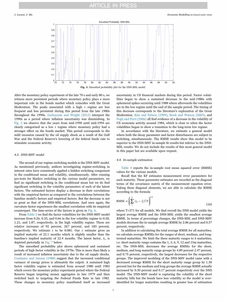
After the monetary policy experiment of the late 70 s and early 80 s, wewitness more persistent periods where monetary policy plays a moreimportant role in the bonds market which coincides with the GreatModeration. The peaks associated with a high λ regime are lessfrequent and less persistent during this period from the late 1980sthroughout the 1990s. Gurkaynak and Wright (2012) interpret the1990s as a period where inflation uncertainty was diminishing. InFig. 5 we observe that the years from mid-1990 until mid-1994 areclearly categorized as a low λ regime where monetary policy had astronger effect on the bonds market. This period corresponds to themild recession caused by the oil supply shock as a result of the GulfWar and the Federal Reserve's lowering of the federal funds rate tostimulate economic activity.

4.3. DNS-MSV model

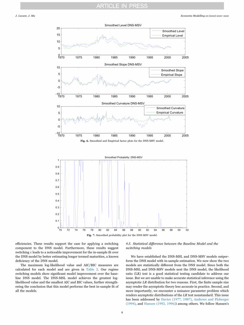
The second of our regime-switching models is the DNS-MSV model.As mentioned previously, authors investigating regime-switching ininterest rates have consistently applied a hidden switching componentto the conditional mean and volatility, simultaneously. After runningpre-tests for Markov switching in the various model parameters, wefind no significant switching in the conditional mean but we do findsignificant switching in the volatility parameters of each of the latentfactors. The estimated factors display a decrease in their correlationswith the empirical factors as compared to the correlations between thebaseline model's factors and empirical factors. But the decrease is notas great as that of the DNS-MSL correlations. And once again, thecurvature factor experiences the smallest correlation with its empiricalcounterpart. The time-series of the factors is given in Fig. 6.

From Table 2 we find the factor volatilities for the DNS-MSV modelincrease from 0.26, 0.33, and 0.66 in the low volatility regime to 0.50,1.21, and 1.87, respectively, in the high volatility regime. These arerelative increases of 92 percent, 267 percent, and 183 percent,respectively. We estimate λ to be 0.081. Our λ estimate gives animplied maturity of 22.1 months which is slightly smaller than thebaseline's implied maturity of 22.4 months. The latent factor, St , isdepicted pictorially in Fig. 7 below.

The smoothed probability plot shows ephemeral and sustainedperiods of high factor volatility in the 1970s. This is more than likely aresult of increased inflation uncertainty due to the oil supply shocks.Cosimano and Jansen (1988) suggest that the increased conditionalvariance of energy prices is ultimately the culprit. A sustained highfactor volatility regime is estimated from around 1980 until 1983which covers the monetary policy experiment period where the FederalReserve began targeting money aggregates in late 1979 and thenswitched back to targeting the Federal Funds Rate in late 1982.These changes in monetary policy manifested itself as increased

uncertainty in US financial markets during this period. Factor volati-lities began to show a sustained decrease in the mid-1980s withephemeral spikes occurring until 1988 where afterwards the volatilitiesare in the low regime until the end of the sample period. The timing ofthis decrease corresponds to the literature's exploration of the GreatModeration. Kim and Nelson (1999), Stock and Watson (2003), andFogli and Perri (2006) all find evidence of a decrease in the volatility ofUS economic activity around 1984, which is close to when the factorvolatilities began to show a transition to the long-term low regime.

In accordance with the literature, we estimate a general modelwhere both the decay parameter and factor disturbances are subject toswitching, simultaneously. The RMSE results show this model to besuperior to the DNS-MSV in-sample fit results but inferior to the DNS-MSL results. We do not include the results of this most general modelin this paper but are available upon request.

4.4. In-sample estimation

Table 4 reports the in-sample root mean squared error (RMSE)values for the various models.

Recall that the KF estimates measurement error parameters foreach maturity. These parameter estimates are recorded as the diagonalterms of the covariance matrix of the measurement equation error.Taking these diagonal elements, we are able to calculate the RMSEaccording to the formula

⎛⎝⎜⎜

⎞⎠⎟⎟∑ y y TRMSE = ( − ) /

T

t t1

21/2

(10)

where T=371 for all models. We find overall the DNS model yields thelargest average RMSE and the DNS-MSL yields the smallest averageRMSE. In terms of percentage changes, the DNS-MSL and DNS-MSVmodels decrease the in-sample average RMSE by 2.86 percent and 0.37percent, respectively.

In addition to calculating the total average RMSE for all maturities,we calculate average RMSEs for the ranges of short, medium, and long-termed maturities. We limit the three maturity ranges to 6 maturities,i.e. short maturity range contains the 1, 3, 6, 9, 12 and 15m maturities,etc. The DNS-MSL decreases the average RMSEs for the short,medium, and long maturity range groups by 4.89 percent 2.47 percent,and 0.75 percent, respectively, the largest decreases for the respectivegroups. The improved modeling of the DNS-MSV model came with adecreased average RMSE for the short maturity range group by 1.30percent but for the medium and long groups the average RMSE actuallyincreased by 0.30 percent and 0.17 percent respectively over the DNSmodel. The DNS-MSV model is capturing the volatility of the shortmaturity bills but the bonds have less volatility so the model is over-identified for longer maturities resulting in greater loss of estimation

Fig. 5. Smoothed probability plot for the DNS-MSL model.

J. Levant, J. Ma Economic Modelling xx (xxxx) xxxx–xxxx

7

efficiencies. These results support the case for applying a switchingcomponent to the DNS model. Furthermore, these results suggestswitching λ leads to a noticeable improvement for the in-sample fit overthe DNS model by better estimating longer termed maturities, a knowndeficiency of the DNS model.

The maximum log-likelihood value and AIC/BIC measures arecalculated for each model and are given in Table 2. Our regimeswitching models show significant model improvement over the base-line DNS model. The DNS-MSL model achieves the greatest log-likelihood value and the smallest AIC and BIC values, further strength-ening the conclusion that this model performs the best in-sample fit ofall the models.

4.5. Statistical difference between the Baseline Model and theswitching models

We have established the DNS-MSL and DNS-MSV models outper-form the DNS model with in-sample estimation. We now show the twomodels are statistically different from the DNS model. Since both theDNS-MSL and DNS-MSV models nest the DNS model, the likelihoodratio (LR) test is a good statistical testing candidate to address ourissue. But we are unable to make accurate statistical inference using theasymptotic LR distribution for two reasons. First, the finite sample sizemay render the asymptotic theory less accurate in practice. Second, andmore importantly, we encounter a nuisance parameter problem whichrenders asymptotic distributions of the LR test nonstandard. This issuehas been addressed by Davies (1977, 1987), Andrews and Ploberger(1994), and Hansen (1992, 1996)) among others. We follow Hansen's

Fig. 6. Smoothed and Empirical factor plots for the DNS-MSV model.

Fig. 7. Smoothed probability plot for the DNS-MSV model.

J. Levant, J. Ma Economic Modelling xx (xxxx) xxxx–xxxx

8

simulation methodology to design a bootstrap procedure using the LRtest.2

We outline the steps used to bootstrap the LR distribution for thecomparison of the DNS and DNS-MSL models:

STEP 1: Obtain the max likelihood value (LLV0) of the DNS model(null) and the max likelihood value (LLVA) of the DNS-MSL model(alternative), using the real dataset. Calculate the LR statistic.STEP 2: Generate yields (y0) using the DNS model. Fit the DNS-MSL and DNS models to the generated yields (y0). Obtain the maxlikelihood value (LLV*A) for the DNS-MSL model and (LLV*0 ) for theDNS model. Calculate the new LR*

j using LLV*0 and LLV*A .

STEP 3: Using LR and LR*j compute a bootstrap critical value (C*

α ).

For a test at level α, first sort the LR*j from smallest to largest. Then

calculate

C LR* ≃ *α α B( +1)

where α represents your confidence level and B is the number of

bootstraps. Repeat steps 2 and 3 B times and obtain LR{ *}jB

1.

STEP 4: Reject the null hypothesis if LR C> *α .

The steps are the same for deriving the LR distribution for the DNSand DNS-MSV comparison.

The LR test statistic under the null of no switching is 467 for theDNS-MSL model and 410 for the DNS-MSV model. We perform 1000bootstraps to derive a LR distribution. Fig. 8 is a plot of the probabilitydensity for both models using a normal kernel function to smooth.

Table 5 lists the critical vales for each model at the 10%, 5% and 1%confidence levels.

It is evident that the test statistic greatly exceeds all bootstrappedcritical values so we are able to reject the null of the linear DNS model.This greatly enhances our stance that term structure modeling shouldtake into account regime switching and that a model without regime

switching is subject to omitted variable bias.

4.6. The relationships of the factors to the macro-economy

A number of papers have tried to establish relationships betweenyield curve factors, such as the NS factors or the first three principalcomponents of the term structure, with macro-factors. We start with alook at correlations between the level and slope factors of our variousmodels with macro-factors inflation expectations and capacity utiliza-tion. Inflation expectations data comes from the University of Michigansurvey in the St. Louis FRED database and covers the period January1978 through December 2000. Capacity utilization which serves as ourproxy for economic activity also comes from the FRED database andcovers the period January 1970 through December 2000. Table 6shows the correlations for the smoothed factors of the DNS, DNS-MSL,and DNS-MSV models and the macro-factors.

Table 4Treasury yields in-sample evaluation: Root Mean Squared Errors (RMSEs).

DNS DNS-MSL DNS-MSVMaturity RMSE RMSE RMSE

1 0.7296 0.6506 0.72743 0.4919 0.4274 0.48406 0.2524 0.2875 0.23029 0.3087 0.3255 0.310112 0.3253 0.3219 0.327215 0.3147 0.2901 0.312318 0.2928 0.2702 0.287021 0.2777 0.2727 0.271924 0.2669 0.2774 0.270430 0.2702 0.2723 0.274136 0.2831 0.2712 0.289048 0.3201 0.3047 0.323360 0.3024 0.2847 0.305972 0.3243 0.3271 0.322384 0.3282 0.3350 0.327896 0.3264 0.3294 0.3249108 0.3879 0.3756 0.3898120 0.4122 0.4140 0.4145Average 0.3453 0.3354 0.34401-15mo 0.4038 0.3838 0.398518-48mo 0.2851 0.2781 0.286060-120mo 0.3469 0.3443 0.3475

Note: The bold-faced RMSEs represent the minimal RMSE for each maturity andmaturity ranges.

Fig. 8. Likelihood Ratio Distributions for the DNS-MSL and DNS-MSV models.

2 Our regime switching methodology is more closely related with Hansen (1992) whentesting in the presence of nuisance parameters than Andrews and Ploberger (1992) whichapply their test in the context of a single break in dynamics.

J. Levant, J. Ma Economic Modelling xx (xxxx) xxxx–xxxx

9

Correlations between inflation expectations and the smoothed levelfactors of the various models are about 0.4. This is a good indicator thatthe level factor is capturing the dynamics of inflation from the late1970s through 2000. The DNS model yields the highest correlation(0.4135) while the DNS-MSL model gives the smallest (0.3982).Correlations between smoothed slope factors and capacity utilizationare about -0.2. The negative correlation here indicates that recessionsare related with a larger magnitude of the slope factor and hencesteeper curve. This tells us that the slope factor is more related withcounter-cyclical monetary policy. In recessions the Fed tends to lowerthe short rate (recall the Taylor rule) and thus steepens the yield curve.Although flatter yield curve tends to predict recessions, steeper curve iscontemporaneously related with recessions. The DNS model gives thelargest absolute value for the correlation (0.1995) while the DNS-MSLgives the smallest absolute value (0.1935).

The investigations of Bansal and Zhou (2002), Clarida et al. (2006),Xiang and Zhu (2013) show a relationship between interest rateregimes and real economic activity. To investigate a similar relation-ship with our regime switching models, we estimate a logit model using

the monthly capacity utilization data as our measure of economicactivity and transform smoothed probabilities from the DNS-MSL andDNS-MSV models into a binary probability variable, yp ( ). The binaryvariable is defined to assume the value of zero when the smoothedprobability value is greater than or equal to one-half and one when lessthan one-half. Thus, we focus on the low regimes. Fig. 9 gives the DNS-MSL smoothed probability plot superimposed on a plot of the inflationexpectations and capacity utilization macro-factors for the period1895–2000.

Fig. 10 gives the DNS-MSV smoothed probability plot superim-posed on a plot of the same macro-factors and time period found inFig. 9.

Fig. 11 is a transformed binary probability plots for the DNS-MSLmodel superimposed on the inflation expectations and capacity utiliza-tion macro-factors.

Fig. 12 gives the DNS-MSV transformed binary probability plotssuperimposed on a plot of the same macro-factors and time periodfound in Fig. 11.

The logit model takes the following form

yCAPUTIL

CAPUTILp

β ββ β

( ) =exp ( + )

1 + exp ( + )low 0 1

0 1

where yp ( )owl is the transformed smoothed probability of being in thelow interest rate level regime for the DNS-MSL model and the lowvolatility regime for the DNS-MSV model.

The sample period we investigate with the logit regressions isJanuary 1985 through December 2000 to mitigate the interest ratevolatility over the period associated with the monetary policy experi-ment of the late 1970s and early 1980s and to take advantage of theeconomic stability associated with the Great Moderation.

In times of low interest rate volatility, manufacturers will increaseplanned investment spending due to the low level of economicuncertainty. Thus we would expect increased economic activity. TheDNS-MSV logit model should reflect this relationship with positivecoefficients for capacity utilization when regressing on transformed lowvolatility regime smoothed probabilities. The DNS-MSV logit modelgives β =1.33(0.59)1 which implies the odds of being in the low volatility

Fig. 9. DNS-MSL smoothed probabilities plotted with inflation expectations and capacity utilization.

Table 5Likelihood Ratio Critical Values (1000 Bootstrap Iterations).

10% 5% 1% LR-stat p-value

DNS-MSL 22.89 37.58 55.18 467 0.00DNS-MSV 24.64 37.06 55.90 410 0.00

Table 6Correlations between macro-factors and estimated factors.

DNS DNS-MSL DNS-MSV

ρLEST ,INFEXP 0.4135 0.3982 0.4103

(0.043) (0.044) (0.043)

ρSEST ,CAPUTIL -0.1995 -0.1935 -0.1984

(0.050) (0.050) (0.050)

Note: INFEXP represents the inflation expectations macro-factor and CAPUTILrepresents the capacity utilization macro-factor. Standard errors are in parentheses.

J. Levant, J. Ma Economic Modelling xx (xxxx) xxxx–xxxx

10

regime increases by 74%. The Mcfadden pseudo-R2 of this regressionwas 0.31.3 Xiang and Zhu (2013) also find a significantly positivecoefficient for their logit model when the low volatility regimeprobabilities are used. This result supports the economic prior thatbeing in a low volatility regime is more likely to occur during aneconomic expansion. Abdymomunov and Kang (2015) further echo thisin finding a decrease in yield volatilities when the monetary authorityimplements “passive” monetary policy during expansions.

The DNS-MSL logit parameter estimates yields interesting resultsthat suggest an asymmetric impact of monetary policy on the yield

curve over the business cycles. The logit regression yields a parameterestimate of β =−0.58(0.11)1 with a pseudo-R2 of 0.15. This estimatetranslates to a 79% decrease in the odds of being in the low lambdaregime. In other words, increasing capacity utilization or an economicboom tends to be associated with the high λ regime, in which the slopefactor has a relatively smaller impact on the yields curve compared tothe low λ regime (recall the bottom left plot of Fig. 4). Since the slopefactor normally approximates the monetary policy this finding suggeststhat the monetary policy seems to have a larger impact on the yieldcurve during recessions than expansions. Once again support for thiscan be found in Abdymomunov and Kang (2015) who show an increasein the term spread due to “active” monetary policy to combatinflationary pressures on economic growth or economic slowdowns.This reveals an interesting asymmetric effect of the monetary policy on

Fig. 11. DNS-MSL transformed binary probabilities plotted with inflation expectations and capacity utilization.

Fig. 10. DNS-MSV smoothed probabilities plotted with inflation expectations and capacity utilization.

3 For the logit regression a sufficient condition for a satisfactorily good model fit iswhen the McFadden pseudo-R2 falls within the interval [0.2, 0.4].

J. Levant, J. Ma Economic Modelling xx (xxxx) xxxx–xxxx

11

the economy through the yields curve.

5. Conclusion

In this paper we investigate and model the parameter instability inthe term structure using regime-switching dynamic Nelson-Siegelmodels. After applying a hidden Markov switching component to allof the model's parameters one at a time, we find that the factor loadingparameter and the factors’ conditional volatilities show significantswitching when allowed—not the conditional mean as noted in theliterature. Specifically, the model allowing switching loading para-meters yields smaller AIC/BIC values and produces smaller root meansquared error values for most of the individual maturities. The modelalso produced smaller RMSEs across maturity groupings, and a smallertotal RMSE. Overall this model gives a more accurate timing of regimeduration in the term structure over the sample period. We also test tosee if both models are statistically different from the non-switchingmodel using a LR test. To correct for non-standard errors due to anuisance parameter issue, we bootstrap critical values for the test. Our

testing results show that both models are statistically different from thenon-switching model at the one percent confidence level, thus support-ing an extension of the DNS model to include regime switchingcomponents.

Finally, we find that the extracted factors from our DNS models areclosely related with the macro-economy. In particular, the level factorappears to be strongly correlated with inflation expectations while theslope factor seems to be counter-cyclical, which is consistent with someprevious findings, such as Wu (2002), that the slope factor may well beclosely related with monetary policy. In addition, we also find that theregime switching in the extended DNS models coincides with economicactivity and monetary policy changes. The model accounting for regimechanges in volatility captured the timing of volatility regimes associatedwith the oil price shock of the 1970s, the monetary policy experiment ofthe early 1980s and the period known as the Great Moderation. Themodel accounting for regime switching in the loading parametersuggests an interesting asymmetric effect of monetary policy on theyield curve. Specifically, we find that the monetary policy tends to havea larger impact on the yield curve during recessions than expansions.

Appendix A. Kalman Filter

Since the DNS model is linear in latent factors, we are able to use the Kalman filter (KF) to estimate the latent factors conditional on past andcontemporaneous observations of the yields. The KF procedure is carried out recursively for t T= 1,…, with initial values for the latent factors andtheir variances being the unconditional mean and unconditional variance, respectively. If we define ft|t as the minimum mean square linearestimator (MMSLE) of Ft and vt|t as the mean square error (MSE) matrix, then f =1|0 μ and v I A Σ=( − ) η1|0

−1 . With observation yt and initial values f1|0and v1|0 available, the KF updates the values for ft|t and vt|t using the equations

f f K e= + ,t t t t t t t| | −1 | −1 (A.1)

v v K vλΛ= − ( ) ,t t t t t t t| | −1 | −1 (A.2)

where e y= −t|t t−1 fλΛ( ) t|t−1 is the predicted error vector, ev vλ λΛ Λ Σ= ( ) ( )′ +t|t t|t ε−1 −1 is the predicted error variance matrix and K =t v evλΛ( )′t|t t|t−1 −1−1 is the

Kalman gain matrix.The next period t + 1 MMSLE of the latent factors and associated variance matrix conditional on yields y y,…, t1 are governed by the prediction

equations

f I A μ Af=( − ) +t t t t| −1 −1| −1 (A.3)

v Av A Σ= ′+ .t t t t η| −1 −1| −1 (A.4)

Fig. 12. DNS-MSV transformed binary probabilities plotted with inflation expectations and capacity utilization.

J. Levant, J. Ma Economic Modelling xx (xxxx) xxxx–xxxx

12

Denote θ as the system parameter vector. The parameters to be estimated via numerical maximum likelihood estimation

are⎧⎨⎩

⎫⎬⎭θ A μ λΣ Σ= , , , ,DNS ij ε ηij ij . We represent the likelihood function as

∑ ∑θ ev e ev eNT log πℓ( )=−2

2 − 12

log | | − 12

′( ) .t

T

tt

T

t t t=1 =1

−1

(A.5)

The function θℓ( ) is evaluated by the Kalman filter through a quasi-Newton optimization method for the purposes of maximization withoutinverting the Hessian matrix of this 28-parameter system.

The values for ft|t and vt|t from the last iteration of the KF are used as initial values in the recursive algorithm to obtain smoothed values of theunobserved factors. Iterating the following two equations backwards for t T T= − 1, − 2, …1, gives the smoothed estimates:

f f v v f f μλ λΛ Λ= + ( )′ ( − ( ) − ),t T t t t t t t t T t t| | | +1|−1

+1| | (A.6)

v v v v v f v vλ λΛ Λ= + ( )′ ( − ) ′ ( ) .t T t t t t t t t T t t t t t t| | | +1|−1

+1| +1| +1|−1 | (A.7)

These smoothed estimates provide a more accurate inference on ft because it uses more information from the system than the filtered estimates.

Appendix B. Kim Algorithm

The Kim algorithm (KA) allows for efficient estimation of parameters through the KF and accurate inference of the realized states through amethodology developed by Hamilton (1989, 1990). For both the DNS-MSL and DNS-MSV models, the transition probabilities between states are

governed by the entries of the matrix⎡⎣⎢

⎤⎦⎥

p p p pp q p q

= =1 −=1 − =00 01

10 11

where p Pr ψ j|ψ i= [ = = ]ij t t−1 with p∑ =1j ij=01 for all i.

The estimation of the model parameters according to the KA is very similar to the KF procedure explained for the non-switching case. Recall thelatent factors for the DNS-MSL and DNS-MSV models are the NS factors and the unobserved state, ψt . We initialize the NS factors and theirvariances as in the non-switching case. To initialize the unobserved state, ψt, we need Pr ψ j|[ = Ω ]0 0 where j = 0,1 and Ωt refers to information up totime t . This expression is the steady state or unconditional probability of being in the low regime which is given by the formulas

π ψ pp q

=Pr[ =0 Ω ]= 1−2− −0 0 0

(B.1)

π ψ qp q

=Pr[ =1 Ω ]= 1−2− −1 0 0

(B.2)

where p and q are defined in the above transition probability matrix. Given realizations of the NS factors at t and t − 1 when ψ i=t−1 and ψ j=t , the KFcan be expressed as

f f K e= + ,t ti j

t ti j

ti j

t ti j

|( , )

| −1( , ) ( , )

| −1( , )

(B.3)

v v K vλΛ= − ( ) ,t ti j

t ti j

ti j

t ti j

|( , )

| −1( , ) ( , )

| −1( , ) (B.4)

e y fλΛ= − ( )t ti j

t t ti j

| −1( , )

| −1( , )

(B.5)

ev evλ λΛ Λ Σ= ( ) ( )′+t ti j

t ti j

ε| −1( , )

| −1( , ) (B.6)

f I A μ Af=( − ) +t ti j

j t ti j

| −1( , )

−1| −1( , )

(B.7)

v Av A Σ= ′+t ti j

t ti j

η| −1( , )

−1| −1( , )

(B.8)

where K =ti j( , ) v evλΛ( )′( )t t

i jt t

i j| −1( , )

| −1( , ) −1 is the Kalman gain

The efficiency of the KA arises from collapsing the (2 × 2) posteriors ft|ti j( , ) and vt|t

i j( , ) into two single-state posteriors

ffPr ψ i ψ j

Pr ψ j=

∑ [ = , = |Ω ][ = |Ω ]t t

j i t t t t ti j

t t|

=01

−1 |( , )

(B.9)

and

vv f f f fPr ψ i ψ j

Pr ψ j{

=∑ [ = , = Ω ] +( − )( − )′}

[ = |Ω ],t t

j i t t t t ti j

t tj

t ti j

t tj

t ti j

t t|

=01

−1 |( , )

|( )

|( , )

|( )

|( , )

(B.10)

by taking weighted averages over states at t − 1. Following Hamilton (1989, 1990), the Kim (1994) algorithm is a consequence of Bayes’ theoremwhich we can use to get the previous single-state posteriors results. Starting with the joint distribution of our states, we have

yy

yy

ψ j ψ iψ j ψ i

Prf ψ j ψ i ψ j ψ i

PrPr[ = , = |Ω ]=

Pr[ , = , = |Ω ][ |Ω ]

=( | = , = ,Ω )×Pr[ = , = |Ω ]

[ |Ω ]t t tt t t t

t t

t t t t t t t

t t−1

−1 −1

−1

−1 −1 −1 −1

−1 (B.11)

The two terms in the numerator and the probability in the denominator can be put in terms of known quantities from our estimation model. Theconditional density yf ψ i ψ j( | = , = ,Ω )t t t t−1 −1 is obtained based on the prediction error decomposition:

⎧⎨⎩⎫⎬⎭y ev e ev ef ψ i ψ j π exp( = , = ,Ω )=(2 ) | | − 1

2′( )t t t t

Nt t

i jt t

i jt t

i jt t

i j−1 −1

− 2 | −1( , )

| −1( , )

| −1( , ) −1

| −1( , )

J. Levant, J. Ma Economic Modelling xx (xxxx) xxxx–xxxx

13

and

ψ j ψ i Pr ψ j ψ i ψ iPr[ = , = |Ω ]= [ = | = ] × Pr[ = |Ω ]t t t t t t t−1 −1 −1 −1 −1

where Pr ψ j|ψ i[ = = ]t t−1 is the transition probability. The terms in the numerator are now in known terms. The denominator, yPr [ | Ω ]t t−1 , can beexpressed as

∑ ∑y y ψ j ψ iPr[ Ω ]= Pr[ , = , = |Ω ].t tj i

t t t t−1=0

1

=0

1

−1 −1(B.12)

Finally, summing over state i we get our single state posterior

∑ψ j ψ j ψ iPr[ = |Ω ]= Pr[ = , = |Ω ].t ti

t t t=0

1

−1(B.13)

From the filter we obtain the density of yt conditional on past information ψt−1, t T= 1,2,…, . We can now calculate maximum likelihood estimatesfrom the approximate log likelihood function

∑θ yln f y y y Prℓ( )= [ ( , ,…, )]= ln ( [ |Ω ]).Tt

T

t t1 2=1

−1(B.14)

Because these are switching models, the parameter vector set for both are going to be have more parameters estimated than the non-switchingmodel: θ A μ λ λΣ Σ={ , , , , , }DNS MSL ij ε η− 0 1ij ij and θ A μ λΣ Σ={ , , , , }.DNS MSV ij ε η− ij ψt ij

Once we have finished calculating the maximum of θℓ( ), all parameters have been estimated and we can get inferences on ψt and ft conditionalon all the information in the sample: Pr ψ j[ = |Ω ]t t and ft|T for t T= 1,2,…, . Instead of incrementing to the end of the sample as in the KF, to obtainsmoothed probabilities and factors we increment from the end of the sample to the beginning, gathering all information along the way. So fort T T= − 1, − 2…,1 we can approximate the smoothed joint probability

ψ j ψ k ψ k ψ ψ jψ k ψ j ψ j ψ k ψ j

ψ kPr[ = , = |Ω ]≈Pr[ = ]×Pr[ = |Ω ]=

Pr[ = |Ω ] × Pr[ = |Ω ] × Pr[ = , = | = ]Pr[ = |Ω ]t t T t T t t

t T t t t t t

t t+1 +1

+1 +1

+1 (B.15)

and probability

∑ψ j ψ j ψ kPr[ = |Ω ]= Pr[ = , = |Ω ]t Tk

t t T=0

1

+1(B.16)

These probabilities are used as weights in weighted averages to collapse the M M( × ) elements of ft|Tj k( , ) and vt|T

j k( , ) into M where M = 2 for ourmodel. These weighted averages over ψt+1 are

ffPr ψ j ψ k

Pr ψ j=

∑ [ = , = |Ω ][ = |Ω ]t T

j k t t T t Tj k

t T|

=01

+1 |( , )

(B.17)

and

vv f f f fPr ψ j ψ k

Pr ψ k{

=∑ [ = , = Ω ] +( − )( − )′}

[ = |Ω ]t Tj k t t T t T

j kt Tj

t Tj k

t Tj

t Tj k

t T|

=01

+1 |( , )

| |( , )

| |( , )

(B.18)

Taking a weighted average over the states at time t we get an expression for the smoothed factors

∑f fψ j= Pr[ = |Ω ] .t Tj

t T t Tj

|=0

1

|(B.19)

This completes the KA. Further details and justifications can be found in Kim and Nelson (1999).

References

Abdymomunov, A., Kang, K.H., 2015. The effects of monetary policy regime shifts on theterm structure of interest rates. Stud. Nonlinear Dyn. Econom..

Andrews, D.W., Ploberger, W., 1994. Optimal tests when a nuisance parameter is presentonly under the alternative. Econom.: J. Econom. Soc., 1383–1414.

Bansal, R., Zhou, H., 2002. Term structure of interest rates with regime shifts. J. Finance57 (5), 1997–2043.

Bekaert, G., Cho, S., Moreno, A., 2010. New Keynesian macroeconomics and the termstructure. J. Money Credit Bank. 42 (1), 33–62.

Bianchi, F., Mumtaz, H., Surico, P., 2009. The great moderation of the term structure ofUK interest rates. J. Monetary Econ. 56 (6), 856–871.

Chauvet, M., 1998. An econometric characterization of business cycle dynamics withfactor structure and regime switching. Int. Econ. Rev., 969–996.

Christensen, J.H., Diebold, F.X., Rudebusch, G.D., 2009. An arbitrage‐free generalizedNelson–Siegel term structure model. Econom. J. 12 (3), C33–C64.

Christensen, J.H., Diebold, F.X., Rudebusch, G.D., 2011. The affine arbitrage-free class ofNelson–Siegel term structure models. J. Econom. 164 (1), 4–20.

Clarida, R.H., Sarno, L., Taylor, M.P., Valente, G., 2006. The Role of Asymmetries andRegime Shifts in the Term Structure of Interest Rates*. J. Bus. 79 (3), 1193–1224.

Coroneo, L., Nyholm, K., Vidova-Koleva, R., 2011. How arbitrage-free is the Nelson–

Siegel model? J. Empir. Finance 18 (3), 393–407.Cosimano, T.F., Jansen, D.W., 1988. Estimates of the variance of US inflation based upon

the ARCH model: comment. J. Money Credit Bank. 20 (3), 409–421.Davies, R.B., 1977. Hypothesis testing when a nuisance parameter is present only under

the alternative. Biometrika 64 (2), 247–254.Davies, R.B., 1987. Hypothesis testing when a nuisance parameter is present only under

the alternative. Biometrika 74 (1), 33–43.Dewachter, H., Lyrio, M., 2008. Learning, macroeconomic dynamics and the term

structure of interest ratesIn Asset Prices and Monetary Policy. University of ChicagoPress, 191–245.

Diebold, F.X., Li, C., 2006. Forecasting the term structure of government bond yields. J.Econom. 130 (2), 337–364.

Diebold, F.X., Rudebusch, G.D., Boragan Aruoba, S., 2006. The macroeconomy and theyield curve: a dynamic latent factor approach. J. Econom. 131 (1), 309–338.

Evans, C. L.Marshall, D. A. (1998, December). Monetary policy and the term structure ofnominal interest rates: evidence and theory. In Carnegie-Rochester ConferenceSeries on Public Policy (Vol. 49, pp. 53–111. North-Holland.

Fama, E.F., Bliss, R.R., 1987. The information in long-maturity forward rates. Am. Econ.Rev., 680–692.

Fogli, A., Perri, F., 2006. The “Great Moderation” and the US External Imbalance (No.w12708) National Bureau of Economic Research.

Garcia, R., Perron, P., 1996. An analysis of the real interest rate under regime shifts. Rev.

J. Levant, J. Ma Economic Modelling xx (xxxx) xxxx–xxxx

14

Econom. Stat., 111–125.Gurkaynak, R.S., Wright, J.H., 2012. Macroeconomics and the term structure. J.

Econom. Lit. 50 (2), 331–367.Hamilton, J.D., 1989. A new approach to the economic analysis of nonstationary time

series and the business cycle. Econom.: J. Econom. Soc., 357–384.Hamilton, J.D., 1990. Analysis of time series subject to changes in regime. J. Econom. 45

(1), 39–70.Hansen, B.E., 1992. The likelihood ratio test under nonstandard conditions: testing the

Markov switching model of GNP. J. Appl. Econom. 7 (S1), S61–S82.Hansen, B.E., 1996. Erratum: the likelihood ratio test under nonstandard conditions:

testing the Markov switching model of GNP. J. Appl. Econom. 11 (2), 195–198.Hevia, C., Gonzalez‐Rozada, M., Sola, M., Spagnolo, F., 2015. Estimating and forecasting

the yield curve using a Markov switching dynamic Nelson and Siegel model. J. Appl.Econom..

Kalman, R.E., 1960. A new approach to linear filtering and prediction problems. J. BasicEng. 82 (1), 35–45.

Kim, C.J., 1994. Dynamic linear models with Markov-Switching. J. Econom. 60, 1–22.Kim, C.J., Nelson, Charles R., 1999. State-Space Models with Regime Switching:

Classical and Gibbs-Sampling Approaches with Applications. MIT Press, Cambridge.Koopman, S.J., Mallee, M.I., Van der Wel, M., 2010. Analyzing the term structure of

interest rates using the dynamic Nelson–Siegel model with time-varying parameters.J. Bus. Econ. Stat. 28 (3), 329–343.

Nelson, C.R., Siegel, A.F., 1987. Parsimonious modeling of yield curves. J. Bus.,473–489.

Startz, R., Tsang, K.P., 2010. An Unobserved Components Model of the Yield Curve. J.Money Credit Bank. 42 (8), 1613–1640.

Stock, J.H., Watson, M.W., 2002. Has the business cycle changed and why? In NBERMacroeconomics Annual, 17 2003 MIT press, pp. 159–230.

Svensson, L.E., 1995. Estimating forward interest rates with the extended Nelson &Siegel method. Sver. Riksbank Q. Rev. 3 (1), 13–26.

Wu, T., 2002. Monetary Policy and the Slope Factors in Empirical Term StructureEstimations,” Federal Reserve Bank of San Francisco Working Paper Series, 2002,2007.

Xiang, J., Zhu, X., 2013. A regime-switching Nelson–Siegel term structure model andinterest rate forecasts. J. Financ. Econom. 11 (3), 522–555.

Yu, W.C., Salyards, D.M., 2009. Parsimonious modeling and forecasting of corporateyield curve. J. Forecast. 28 (1), 73–88.

Yu, W.C., Zivot, E., 2011. Forecasting the term structures of Treasury and corporateyields using dynamic Nelson-Siegel models. Int. J. Forecast. 27 (2), 579–591.

J. Levant, J. Ma Economic Modelling xx (xxxx) xxxx–xxxx

15

本文献由“学霸图书馆-文献云下载”收集自网络，仅供学习交流使用。

学霸图书馆（www.xuebalib.com）是一个“整合众多图书馆数据库资源，

提供一站式文献检索和下载服务”的24 小时在线不限IP

图书馆。

图书馆致力于便利、促进学习与科研，提供最强文献下载服务。

图书馆导航：

图书馆首页 文献云下载 图书馆入口 外文数据库大全 疑难文献辅助工具