A Dynamic Model of Elementary School Choice

Autores: Nicolas Grau

Santiago, Enero de 2016

SDT 417

A Dynamic Model of Elementary School Choice

Nicolas Grau∗

June 2015

Abstract

This paper builds and estimates a dynamic model of elementary school choice us-ing detailed Chilean administrative data. In the model, parents care about differentfeatures of primary schools: school’s socioeconomic composition, quality (measuredas the school’s contribution to standardized test scores), religiosity, location, typeof administration, tuition fee and GPA standard. Parents are heterogeneous in twodimensions: whether they have the skills needed to understand public informationabout quality (standardized tests), and their involvement in their child’s school. Theresults suggest that: (1) Parents care about school quality, but to a moderate degree.(2) Parents have an important misperception about school quality, which results in aless favorable opinion about the quality of public schools, relative to private schools.(3) If parents were only concerned about quality, they would choose public schoolsmore often. (4) Admission restrictions play a relevant role; otherwise, parents wouldchoose private school more frequently.

JEL Classification(s): I24, C35, D03

I thank the Chilean Ministry of Education for providing the data. I am very grateful to Diego Amador,

Flavio Cunha, Francisco Gallegos, Petra Todd, Kenneth I. Wolpin, and seminar participants at the North

American Summer Meetings of the Econometric Society (University of Minnesota), Universidad de Chile,

Univesidad Catolica de Chile, Universidad de Santiago, and UDP for helpful comments and suggestions.

I also thank the Centre for Social Conflict and Cohesion Studies (CONICYT/FONDAP/15130009) for

financial support.

∗ngrau@fen.uchile.cl. Department of Economics, University of Chile and Centre for Social Conflictand Cohesion Studies (COES)

1

1 Introduction

A frequent topic in policy debates is what should be the role – if any – of marketincentives in education provision. Given that parents’ choice is the critical mechanismto increase school quality in a market-oriented educational system, the literature hasfocused on the extent to which parents consider school quality when they make theirdecisions, and how this consideration is heterogeneous across parents. To understandparents’ school choice, and the potential heterogeneity in their preferences, one mustseparate the effects of differences in their preferences, in perceptions about quality, andin choice sets. Distinguishing these three elements is a complex task given that, ingeneral, these determinants of parents’ choice are not observable.

In this paper, I build and estimate a dynamic model of elementary school choice. Tothis end, I use detailed Chilean administrative data for the students who entered 1stgrade in 2004. As many authors have emphasized (e.g., Gallego and Hernando (2008)and Hsieh and Urquiola (2006)), the Chilean system is probably the most massive schoolchoice program in the world, hence the importance of studying the determinants of schoolchoice in this context.

I model elementary school choice at the end of each academic year, allowing for parentalheterogeneity along several dimensions: their ability to understand public informationabout quality (standardized tests), how much they care about school quality (measuredas the school’s contribution to standardized test scores), their involvement in the schoolattended by their child, and their choice set.1 By estimating the structural parameters ofthe model, I am able to assess the empirical relevance of these components in explainingboth the observed preference for private over public schools and the unequal access tohigh quality schools.

In the model, parents care about different characteristics of primary schools, such asthe school’s socioeconomic composition, quality, religious affiliation, location, type of ad-ministration (i.e., public, subsidized private and non-subsidized private), tuition fee, andGPA standard (i.e., grading standard). Parents do not perfectly observe school quality.To estimate the quality of each school, they can access two different sources of informa-tion. First, every year they observe the performance of each school on a standardizedtest, which is made public with a one year lag. Parents can have different levels of mis-perception in processing this information; because test scores depend on school qualityand on the socioeconomic status (SES) of the school, parents can confound these twoeffects, confusing high quality schools with schools that have higher SES students. Sec-ond, parents also differ in their exogenous level of involvement in the schooling processof their child, which implies that those who are involved in their child’s school observethe quality of that particular school without misperception.

I estimate the parameters of the model by simulated maximum likelihood, using theMonte Carlo integration and interpolation method (Keane and Wolpin (1994)). To build

1In Chile, at least in my sample period, schools were allowed to select students based on academicand non-academic characteristics (e.g., parents’ marital status).

2

the database of students, I use the administrative panel data from 2004 to 2011, whichincludes the school attended by each student in each year, their average grade, themunicipality where they live and where the school is located, and some basic demographicinformation. Because the sample of students entering 1st grade in 2004 took the SIMCEtest in 4th grade (2007) and in 8th grade (2011), I merge this panel with informationfrom parent surveys associated with those rounds of SIMCE administration, includingmother’s and father’s information. To build the database of schools, I use the test scoresfrom the SIMCE test and the information collected from SIMCE parents’ surveys forthe years 2002, 2005-2011.2 Test scores are used to estimate school quality for everyyear. The surveys include questions about school tuition fees, and information aboutthe elements considered by the school in the admission process. Furthermore, fromadministrative data of the Ministry of Education, I collect information about schools’religious affiliation, if any.

The results show that parents do care –but in a moderate way– about school quality,that more involved parents care marginally more about school quality, and that parents’decisions are not sensitive to quality after the first decision (1st grade). Moreover, theresults also suggest that parents have an important misperception about school quality,which results in a less favorable opinion about the quality of public schools, relative toprivate schools. This result supports the idea that parents may have difficulties in isolat-ing a school’s quality from its socioeconomic composition when they observe test scores.However, given that quality is not very relevant for their decision, such a misperceptiononly partially affects parents’ choices.

Regarding the debate about why parents choose private schools over public schools, theresults show that, if parents were only concerned about quality, they would choose publicschools more often. The same would be true if they did not have a misperception aboutquality. However, the results suggest that admission rules are binding restrictions andthat relaxing them would increase the demand for private schools. The simulationsalso show that schools’ admission rules and household location are both important inexplaining the rise in the achievement gap between students from different SES.

The paper has three main contributions. First, to the best of my knowledge, this is thefirst paper that structurally estimates a dynamic model of elementary school choice. Thedynamic nature of school choice has particular relevance in the Chilean context, wherearound 30% of the students switch schools at least once between 1st and 8th grade (ex-cluding those who moved to other municipalities and those who fail at least one year).Second, the structural approach followed in this paper allows me to quantify differentcauses of unequal access to high quality schools and of the higher demand for privateschools than for public schools. Finally, the model considers the difficulties that par-ents may have in processing and understanding information about school quality, whichcontributes to the scarce literature on structural estimation with bounded rationality, aswell as to the literature that uses observed choices to infer agents’ information.

24th grade SIMCE for years 2002, 2005-2009 and 8th grade SIMCE for years 2004, 2007, 2009 and2011.

3

The structure of the paper is as follows: Section 2 presents a review of the related lit-erature; Section 3 briefly describes the Chilean educational system; Section 4 introducesthe model; Section 5 discusses the data and the procedure to estimate the model; andSection 6 presents the results and the analysis of the counterfactual experiments. Section7 concludes.

2 Literature Review

This paper is related to several strands in the literature. First of all, it is related to thepapers that evaluate the role of competitive market incentives in education provision. Onone side, there are theoretical papers, such as Epple and Romano (1998), and McMillan(2004), which debate the potential for those incentives, specifically tuition vouchers, toincrease schools’ quality and to make significant improvements for poor families.3 On theother side, there are empirical studies that show mixed evidence regarding this debate;see, for example, Hsieh and Urquiola (2006), and Angrist et al. (2006).4

Authors have studied the determinants of parents’ school choice because this is one ofthe important mechanisms that could explain the shortcomings in the implementation ofmarket-oriented policies in education. In particular, they have studied whether and towhat extent parents consider school quality when they make their choice.5 For instance,in an interesting paper, Hastings and Weinstein (2008) used a natural experiment and afield experiment that provided direct information on school test scores to lower-incomefamilies in a public school choice plan, finding a significant increase in the probabilitythat those families would choose higher-performing schools. In an alternative strategy,several studies have focused on estimating the value that parents place on school qualityby calculating how much more people pay for houses located in areas with better schools(e.g., Black (1999) and Kane et al. (2006)).

One caveat about this literature is that, in general, it measures school quality usingaverage school test scores. The problem with this approach is that, from the point ofview of the parents, this average is not relevant; what is relevant is what their child’sperformance would be if she were to attend a particular school. Given that sorting isa common feature in education, these two conditional expectations should not coincide.Exceptions to this general problem are shown in Mizala and Urquiola (2013), Neilson(2013), and Rothstein (2006). For instance, Mizala and Urquiola (2013) use a sharpregression discontinuity to estimate the effect that being identified as a SNED winner(a program which seeks to identify effective schools, controlling for schools’ SES) has on

3In a survey of this literature, Epple and Romano (2012) conclude: Research taking account of distinc-

tive features of the education“market” has shown that early arguments touting the virtues of laissez-faire

flat-rate vouchers were overly optimistic. However, the research does not vindicate voucher opponents

who use shortcomings of the laissez-faire voucher to justify the wholesale dismissal of vouchers.4Bettinger (2011) reviews the cases of Chile, Colombia, and Sweden, emphasizing the context-specific

nature of the results.5See for example Alderman et al. (2001), and Bast and Walberg (2004).

4

schools’ enrollment, finding no consistent evidence that winning a SNED award affectsthis outcome.6

Several authors study the determinants of school choice in the Chilean context.7 Forinstance, Gallego and Hernando (2008), using a semi-structural approach, find resultsthat suggest that the school choice implemented in Chile increased overall student wel-fare, but they also find that there is a lot of heterogeneity in the size and even the signof the welfare change. Along the same lines, Chumacero et al. (2011), using a databasethat accurately estimates the distance between the household and school, find that bothquality and distance are highly valued by households. In a recent and novel paper,Neilson (2013) studies the effects of targeted school vouchers on the outcomes of poorchildren in Chile; his findings suggest that this program effectively raised competition inpoor neighborhoods, pushing schools to improve their academic quality. Finally, Market al. (2006) study how parents construct their school choice sets and comparing this towhat they say they are seeking in choosing schools. Their results indicate that parentaldecisions are influenced by demographics.8

This paper is also related to the literature that models individuals’ economic decisionsincorporating bounded rationality. In general, this literature follows the idea that, asSimon (1986) points out, cognitive effort is a scarce resource, and the knowledge andcomputational power of the decision-maker are always limited. In an interesting paper,which is one of the few papers that perform a structural estimation with bounded ra-tionality, Houser et al. (2004) develop a Bayesian procedure for classification of subjectsinto decision rule types in choice experiments, finding that, in a very difficult dynamicproblem, more than a third of the experimental subjects followed a rule very close to theoptimal (expected wealth maximizing) rule.

Because school choice is a complex task, which involves gathering and processing in-formation, different authors have studied the presence of bounded rationality in thatcontext. For instance, Schneider et al. (1998) find that, on average, low-income parentshave very little accurate information about objective conditions in the schools.9 How-ever, even though levels of objective information held by parents are low, their actualchoice of schools reflects their preferences in education. Along the same lines, Azmat andGarcia-Montalvo (2012) conclude that, as well as parents’ education, information gath-ering and information processing are important determinants for the quality of school

6Mizala et al. (2007) present evidence indicating that, in the case of Chile, once we control for thestudents’ socioeconomic status, the remaining part of the test scores are very volatile from year toyear. Hence, they argue that producing a meaningful ranking of schools that may inform parents andpolicymakers may be harder than is commonly assumed.

7Chile’s school choice policies will be described in the next section.8There are several studies that try to study the effect of the voucher system implementation in Chile.

Although the evidence is mixed regarding its effect on school quality, there is more agreement on thenegative effect of this policy on student socioeconomic segregation (Auguste and Valenzuela (2006); Gauri(1999); and Hsieh and Urquiola (2006)). In a different approach, Bravo et al. (2010) find that educationalvouchers increased educational attainment, high school graduation, college attendance and graduation,and wages.

9The same is found by Henig (1996).

5

choice.

Finally, this paper is also related to the literature that attempts to infer agents’ infor-mation using observed choices, such as: Carneiro et al. (2003); Cunha et al. (2005); andNavarro (2011).

3 The Chilean Educational System

In 1981, the Chilean military government created a voucher market in the educationalsystem, which was part of a broader reform that also included the decentralization ofpublic schools (which were transferred to municipalities) and the introduction of flexi-bility in teachers’ contracts.10 This reform transformed the way schools were funded bythe government, establishing a system where private and public schools were paid perstudent, with a flat voucher, on the basis of attendance.

Since then, the allocation of public resources has been mainly determined by parents’decisions. However, in practice, this decision has had several restrictions: schools canselect students based on their previous performance, tests, and the characteristics oftheir parents (e.g., marital status and religion). On top of that, since 1994, when aco-payment law was passed, schools that are eligible for public funding can also chargea tuition fee; in that case, depending on the amount charged, there is a discount to theschool’s subsidy.11

This reform consolidated a system of mixed provision of education, with three typesof schools; municipal (public), private subsidized (voucher-private), and entirely private(non voucher-private). The first two receive most of their funds from state vouchers,and, since 1994, privately subsidized schools may additionally charge a tuition fee. In2013, over 90% of the Chilean students received funding via vouchers.12

In order to guide parents’ decisions and to measure the student learning process, a newtesting system, SIMCE, came into existence in 1988. The SIMCE is an annual nationwidestandardized test. Its results have been public information for more than two decades,publicized in part by listings in major newspapers of individual schools’ performance.The government also uses SIMCE scores to allocate resources.13

More than 30 years after the reform, there are several clear stylized facts. First, therehas been a massive migration from public to private schools. Indeed, the student fractionin the public system went from 78%, in 1981, to 38% in 2012.14 Secondly, enrollment in

10For a summary of these reforms, see Gauri (1999) and Mizala and Romaguera (2000).11Epple and Romano (2008) emphasize the consequences of this selection mechanism for the outcomes

of an educational voucher system.12Source: Ministry of Education, Chile.13Meckes and Carrasco (2010) describe SIMCE’s main features, purposes, institutional framework, and

strategies for communicating results.14There is a debate, and mixed evidence, about whether voucher private schools have higher quality

than public schools. In a meta-analysis, Drago and Paredes (2011) find that voucher-private schools havea small advantage over public schools. On the contrary, Bellei (2009) finds that voucher-private schoolsare no more effective than public schools, and that they may be less effective.

6

voucher-private schools was accelerated after passage of the co-payment law.15 Thirdly,the magnitude of socioeconomic school segregation is very high (and higher than thegeographical segregation), and has increased slightly over the last decade (Valenzuelaet al. (2014)). Finally, despite important increases in the public budget allocated toeducation, Chile’s performance is relatively poor when compared with similar countries(Chumacero et al. (2011)).

Another salient feature of the Chilean system, which is consistent with its “free choice”design, is that a fairly large number of parents switch schools at some point duringprimary school. In this regard, Table 10 of the Appendix A shows that, in any grade,around 4-7% of the parents change their child’s school, and that more educated parentsare more likely to do so.16 Moreover, Table 9 of the Appendix A shows that more than30% of parents changed their child’s school at least one time during primary school.17

4 The Model

I consider a model in which each family i ∈ 1, 2, ..., I decides among their possibleelementary school alternatives in each of T (finite) discrete periods of time, where T isthe end of the elementary cycle. The educational market is composed of J schools. Theparents’ decision is restricted in two ways. First, each parent i, has a specific choice setΛi ⊆ 1, 2, ..., J. The cardinality of Λi is denoted by S(Λi). Second, each school j ∈ Λi

may or may not admit the student i based on a rule that will be described below.

4.1 Parents’ Utility

Let Dit ∈ Λi be the school chosen by parent i at time t. The flow utility of parents iwhen their child is attending school j at time t is given by:

uijt = βyYjt + βzZij + βgGijt + C 1(Dit−1 6= j) + βeg[Gijt−1 − Gijt−1] (1)

1(Dit−1 = j) + ǫuijt

where Yjt is a vector of characteristics of the school j, including socioeconomic com-position (dummies for 5 tiers), tuition fee, and type of administration (public, voucher-private, and non voucher-private);18 Zij is a vector of variables which are determined bythe relationship between the school j and the individual i, including religion (a dummyvariable which takes one if the school is religious and parents profess a religion, and zero

15See Larranaga (2004).16These figures do not include parents who change the municipality where they live, or students who

repeat a grade. If one considers those cases, this fraction rises to around 11% (Zamora (2011)).17These levels of student mobility are similar to what is observed in other countries. For instance,

Hanushek et al. (2004) show that, in Texas’ public schools, one-third of all children switch schools atleast once between grades 4 and 7, excluding changes due to the transition from elementary to middleschool.

18Given that some prestigious public schools begin at 7th Grade, I also include a dummy variable forthose schools.

7

otherwise), years that student i has been attending school j, and location (a dummyvariable which takes one if the school and the family house are located in different mu-nicipalities, and zero otherwise), Gijt is the GPA obtained by the student, C is the

direct cost of changing school, 1(A) is a function that takes 1 when A is true, Gijt−1

is the expected GPA given the information at t − 2, and ǫuijt is an iid shock. The term

[Gijt−1 − Gijt−1] is included in the utility function to capture that students may preferto stay in their current school when their performance in the previous grade was abovetheir prediction.

This model requires a cost of switching schools, C, in order to fit the patterns of thedata. Otherwise, the model would predict a higher probability of changing schools thanactually exists. However, and beyond this practical consideration, it is reasonable toassume such a cost. Indeed, in the estimation, this parameter will capture an averageof different costs that parents face when they change schools, namely, the student’sadaptation cost,19 and the monetary cost (many schools charge an enrollment fee).

In the final period, there is a utility that also captures all future payoffs, such that

uijT = βTKiKijT + βyYjT + βzZij + C 1(DiT−1 6= j) + βeg[GijT−1 − GijT−1] (2)

1(DiT−1 = j) + βTs SECj + βTagGijT + βTtaTAiT + ǫuijT ,

where KijT is the knowledge achieved by student i in school j at time T , TAiT representsthe time, in years, that student i has been attending the current school and SECj takesone when school j also offers secondary level grades (from 9th to 12th) and zero otherwise.Including the latter in the terminal utility captures the changing costs that parents areforced to incur in T+1 when their child attends a school that does not offer the secondaryclass level. Furthermore, GijT and TAiT are included because, as will be noted, theydetermine the future chances of being admitted in the desired high school.

4.2 Student knowledge

I model student knowledge as a cumulative process. In particular, let qjt be the qualityof school j at time t and qijt the quality of the school attended by student i at time t,

such that qijt =∑J

j=1 qjt1(Dit = j); thus, the learning process is given by:

Ki0 = α0Xi, (3)

Kijt = Kijt−1 + α1qijt.

19The model, as is explained below, also has an explicit cost of switching schools, which is given by thefact that the GPA in school j is, among other things, a function of the time that the child has attendedthat particular school j. The economic literature has found evidence of this pedagogical cost. See, forexample, Hanushek et al. (2004). Thus, C captures the adaptation costs, which come in addition to thiscost in performance.

8

Therefore, the knowledge achieved by student i in school j at time t, Kijt, is a functionof student i’s previous knowledge and the quality of the school she attends that year,qijt. In addition, the initial knowledge only depends on student i’s characteristics Xi

(i.e., parents’ education). It should be noted that in the model, school quality qijt maychange over time, this possibility is also considered in the estimation part.

4.3 GPA function

Grades in elementary school are determined by the following production function:

Gijt = λt0j + λt1jKijt + λt2TAit + εgijt, (4)

This specification captures the idea that each school may have a particular way to mapknowledge onto grades. In particular, the higher the value of λt0j , the more likely it is thatstudents perform well in school j. Moreover, even conditioning on student knowledge,TAit has an effect on grades. This accounts for the fact that it may take time for newstudents to learn the characteristics of the evaluation system of each school. As notedabove, this implies an explicit cost of switching, given that moving to a new school willimply a cost in GPA performance.

Regarding parents’ information, I assume that parents know λt0j , λt1j ∀ t, j, which is

necessary to forecast GPA performance of their children. Intuitively, and this means thatparents know the level of difficulty of any school.

4.4 Probability of admittance

Parents are restricted in their choices to the extent that schools have the right of ad-mittance. Let ADijt be a binary variable, which is unobservable for the econometrician,that equals one if student i can enter school j at time t and zero otherwise, such that:

ADijt =

1 if ijt − εadijt ≥ 0

0 if ijt − εadijt < 0(5)

where

ijt = ϕ0 + ϕqqjtSeljt + ϕ0kSelkjt + ϕ1kKit−1Sel

kjt + ϕ0gSel

gjt + ϕ1gGit−1Sel

gjt (6)

+ ϕ0mrSelmjt + ϕ1mrMRijt−1Sel

mjt + ϕ0rSel

rjt + ϕ1rRELiSel

rjt + ϕsSel

ojt

+ ϕ0nsNewjt + ϕ1nsNewjt ∗ Sizejt + ϕfeXi ∗ feejt + ϕsxXi ∗ Seljt.

and Selkjt takes one when school j selects students based on academic tests and zerootherwise; Selgjt takes one when school j selects students based on previous grades andzero otherwise; Selrjt takes one when school j selects students based on students’ religionand zero otherwise; takes one when school j selects students based on parents’ marital

9

status and zero otherwise Selmjt ; Selojt takes one when school j selects students based on

other reasons and zero otherwise; Seljt is an index to measure how selective is school jat time t.2021 These variables may all equal one at the same time. Newjt takes one whenthe school is new (or doesn’t offer the previous grades), Sizejt is the size of this newschool, and feejt denotes the tuition fee. Finally, MRijt takes one if parents are marriedand zero otherwise, and RELi takes one if parents are religious and zero otherwise.22

Then, assuming that εadijt are iid, following a logistic distribution, the probability ofadmission is described by:

Pr(ADijt = 1) =exp(ijt)

1 + exp(ijt)(7)

To have a tractable likelihood calculation, I assume that εadijt is realized before parents

make the Dit decision.23 Moreover, to simplify the solution of the model, I assume that,

for any student, there is always at least one school willing to admit her.24 In particular,

h ∈ argmaxj∈Λi(ijt) ⇒ ADiht = 1. (8)

I chose this specification for the random process of ADijt for two reasons: given the richinformation that I have about the admission rules of each school, and considering thechallenge in separately identifying the parameters of this process and the parametersof the utility function, when ADijt is latent. In this regard, it should be noted thatthere is no variable that enters in the same way in the admission probability functionand in the utility function.25 For instance, the admission probability is also a functionof the interaction between the tuition and the parents’ socioeconomic status. This isincluded to capture the fact that some tuition is unaffordable to some families. Notethat tuition is also present in the utility function, but this variable only interacts withparents’ socioeconomic status in the admissions probability. Thus, the idea of the firstelement is to capture the fact that parents do not like to pay high prices. The idea of thesecond is to capture the fact that some prices are impossible for some families to pay.

20In the empirical implementation, all these variables are proportions, instead of binary variables. Thisis because I construct these variables from parents’ surveys, and in each school their answers are notalways the same. Thus, for instance, in the empirical implementation, Selkjt is the fraction of parents inschool j who affirm that school j selects students based on an academic test.

21In the empirical implementation of this model, Seljt = (Selkjt + Selgjt + Selojt) ∗

13.

22Contreras et al. (2010) present evidence indicating that student selection is a widespread practiceamong private subsidized schools.

23This means parents do not apply to schools. Instead, at the end of each period they know theirfeasible set for the next period and they pick the feasible school that maximizes their expected utility.

24Given that in the data the argmaxj∈Λi(ijt) is almost certainly a public school (because most of

those schools do not select students), this assumption is equivalent to assuming that there is one publicschool that admits the student i without uncertainty. Which is actually the way that it works in reality.

25The few variables that are in both functions are interacting with other variables in the function thatdetermine the probability of admission.

10

Moreover, this specification takes advantage of the interaction between the features ofthe model and data availability. For instance, if the school selects students based onan academic test (with ϕ1k > 0, as expected), then the higher Kit−1, the higher theprobability of i being admitted at j.

Note that students who decide to stay in their current school do not have to complete anadmissions process. If they want, they can stay in their current school with probability1.

4.5 Parents’ information and perception about quality

Parents have two sources of information about school quality. Firstly, they observe theresults of the standardized tests for all the schools, which is public information. Secondly,they may observe the quality of the school which their child is attending, which is privateinformation.

Regarding public information, it is assumed that standardized tests are measures ofschool quality, whose values also depend on the characteristics of the student. Thus, inthis model, school quality (q) is defined as a school’s contribution to learning, such that:

STχijt = qjt + θ2Xi + ε

χijt, (9)

where STχijt denotes the standardized test score in subject χ, such that

χ ∈ Math, Spanish,Natural Science, Social Science.

In this context, I define qjt as the fixed effect estimation of the expected quality of schoolj at time t, given the public information STjt.

26 Hence, qjt is the unbiased estimate ofqjt given public information at t.27 To the extent that the demographic composition ofthe schools students’ matter for test scores, these peer effect will also be included in qjt.Thus, qjt is in practice the average test score in the school that is not explained by theindividual characteristics of the students (teachers, infrastructure, school manager, etc.).

Although school quality may vary over time, I assume that parents have no informationabout the evolution of quality. Thus, for them the best estimate of future quality is theirestimate of current quality.28

The model is flexible in terms of how parents access and understand the informationabout schools’ quality. In the first place, there are different types of parents with regardto their ability to distinguish the school’s contribution from the students’ contributionto test scores. In the second place, there are different types of parents with regardto their involvement in the schooling process of their child, which determines whether

26The same approach to estimate school quality is followed by Neilson (2013).27X is a matrix with the characteristics of all the students. In practice, to estimate qjt, we only need

the characteristics of parents who send their child to school j.28When I estimate the model, I estimate school quality of year t using only information for that year.

Thus, the estimation approach is totally agnostic to any kind of dynamics.

11

they observe the quality of that school. Namely, only involved parents have access toprivate information. The first is denoted parent’s cognitive skill, whereas the second isdenoted parent’s school involvement. The school involvement type of parent i is givenby ψi ∈ 0, 1, where 1 means involved.29

To present how parents access and understand the information about the quality ofschools, I divide the analysis into three cases: (1) their perception about the qualityof the schools not attended by their child; (2) the involved parents’ perception aboutthe quality of the school attended by their child; and (3) the non-involved parent’sperception about the quality of the school attended by their child. In all three cases,what matters is parents’ perception at the end of t − 1 (when they make the choice ofschool for period t), about school quality at time t, given their information at time t− 1,i.e. Et−1[qjt|Dit−1, ψi].

30

Case 1: Schools not attended by their child.

Et−1[qjt|Dit−1 6= j] = qjt−2 +∑

χ∈A

ηiχ(STχjt−2 − qjt−2), (10)

where, ηiχ = η11,χXi + η2,χS(Λi) and A = m, s, n, sc. Thus, η depends on the par-ents’ education and the size of the choice set (S(Λi)), where the latter is motivated bythe bounded rationality literature.31 Indeed, the way in which the complexity of theinformation processing to make decisions increases the probability of making mistakes iswell-established in that literature. Moreover, in the context of my model, it is rather nat-ural to think that the larger the choice set, the higher the complexity of the informationprocessing. In short, in this model, bounded rationality implies that parents differ in theirability to perceive school quality information correctly, and that their misperception isa function of their educational level and the size of their choice set.

In this case, if as expected ηiχ ≥ 0, then parents will overestimate the quality for schoolswhose students have, on average, highly educated parents.32 Moreover, given the factthat in the Chilean educational system standardized tests are published one year aftertaken, even if parents did not have a misperception about quality (i.e., η = 0), when theychoose the school for time t (at the end of t − 1), they would estimate school qualitiesusing the public information at t− 2.

In sum, the use of public information presents two potential drawbacks: it is publishedafter a delay, and parents may have difficulties in interpreting it, namely, when they ob-

29This is an exogenous, time invariant, parents’ characteristic and therefore it does not depend on theschool’s characteristic.

30I am assuming that parents do not use past grades as a potential source of information to infer schoolquality.

31A survey can be found in Conlisk (1996).32Given the functional form of the standardized tests, ST

χ

jt−2− qjt−2 is the part of the average test, ofsubject χ, that is not explained by school quality. Hence, this is the part explained by the socioeconomiccomposition of the school.

12

serve the tests, they can have problems in isolating school quality from the socioeconomiccomposition of its students.

Case 2: School attended by their child, when parents are involved in that school (ψi =1).33

Et−1[qjt|Dit−1 = j, ψi = 1] = qjt−1 (11)

Thus, parents who are involved in their child’s school observe the quality of that schoolwithout distortion and without lag.34

Case 3: School attended by their child, when parents are not involved in that school(ψi = 0).

Et−1[qjt|Dit−1 = j, ψi = 0] = qjt−2 +∑

χ∈A

ηiχ(STχjt−2 − qjt−2), (12)

A = m, s, n, sc.

Thus, parents who are not involved in their child’s school have, for that school, the sameinformation that they have for all the other schools (public information).

In this context, parents’ perception about their child’s knowledge is given by the followingexpressions:

• E0[Ki0|ψi] = Ki0.

• Et[Kit|Dit, ψi] = Et[Kit−1|Dit, ψi] + α1∑J

j=1Et[qjt|Dit, ψi]1(Dit = j).

• Et−1[Kit|Dit−1, ψi] = Et−1[Kit−1|Dit−1, ψi] + α1∑J

j=1Et−1[qjt|Dit−1, ψi]1(Dit =j).

I denote Kait = Ea[Kit|Dia, ψi], a = t− 1, t.

4.6 Decision Timing and Solution of the Model

At the end of period t − 1, the following random variables are realized: (1) Utilityidiosyncratic shocks: ǫuijt ∀i, j; (2) the right of admittance shocks: εadijt (hence, ADijt)

∀i, j; and (3) test scores, published with lag: STmt−2,ST

lt−2,ST

nt−2,ST

sct−2. Given this

33I allow for βki being different for this type of parent.34This assumption is supported by the evidence presented in Azmat and Garcia-Montalvo (2012), who

find that knowing about and/or visiting more schools is related to more accurately assessing local schools.

13

information, parents decide Dit, taking into consideration the expected flow utility at tand the expected future payoff associated with each school.35

The model is solved by backward recursion, where the dynamic decision is driven by thestate variables (Ωit).

36

Ωit =

Dit, TAit, Ktijt, Gijt, qijt,STt−1, ε

ad

it, ǫu

it if ψi = 1

Dit, TAit, Ktijt, Gijt,STt−1, ε

ad

it, ǫu

it if ψi = 0

(13)

I define Ω−it as the state variables which are observed by the econometrician, such that:37

Ω−it =

Dit, TAit, Ktijt, Git, qijt,STt−1 if ψi = 1

Dit, TAit, Ktijt, Git,STt−1 if ψi = 0

(14)

To consider the school’s right of admittance, I redefine the flow utility as:

uijt = uijt(ǫadijt) + ǫuijt (15)

where,

uijt(ǫadijt) =

βxYjt + βzZij + βgGijt + C 1(Dit−1 6= j)

+βeg[Gijt−1 − Gijt−1]1(Dit−1 = j) if ADijt(Ω−it−1, ǫ

adijt) = 1

−∞ if ADijt(Ω−it−1, ǫ

adijt) = 0

(16)

The solution to this dynamic problem is fully characterized by the integrated valuefunction, V (Ω−

it−1), such that:38

V (Ω−it−1) =

∫maxj∈Λi

Et−1uijt(ǫ

adijt) + ǫuijt + δEt−1[V (Ω−

it)|Ω−it−1,Dit = j]

dGε(εit), εit = [ǫuit ǫ

adit ]

′.

(17)

Then, defining the auxiliary function v(Ωit−1,Dit = h) as:

35εgijt is realized after the decision of Dit is made.

36TAit = 1 + 1(Dit = Dit−1)TAit−1 and Gijt =Gijt−1∗(t−1)+Gijt

t.

37Observed conditional on types.38ǫuit = ǫuijtj∈Λi

and ǫadit = ǫadijtj∈Λi

.

14

v(Ωit−1,Dit = h) = Et−1uiht(ǫadit ) + ǫuiht + δEt−1[V (Ω−

it)|Ω−it−1,Dit = h] (18)

⇒ Dit ∈ argmaxj∈Λiv(Ωit−1,Dit = j) ∀t ∈ 1, 2, ..., T − 1

At the end of T − 1:

uijT (ǫadijT ) =

βKKijT + βxYjT + βzZij + βeg[GijT−1 −GijT−1]1(DiT−1 = j)

+C 1(DiT−1 6= j) + βTs SECj + βTagGijT + βTtaTAiT if ADijt(Ω−iT−1, ǫ

adijT ) = 1

−∞ if ADijt(Ω−iT−1, ǫ

adijT ) = 0

(19)

v(ΩiT−1,DiT = j) = ET−1uijT (ǫadiT ) + ǫuijT , (20)

⇒ DiT ∈ argmaxj∈Λiv(ΩiT−1,DiT = j) .

Thus, using equation 20, it is possible to solve the maximization in the last period. Then,using Monte Carlo integration and interpolation method (Keane and Wolpin (1994)), itis possible to approximate V (Ω−

iT ) for any value of vector Ω−iT , which allows me to solve

the maximization in the period T − 1 (see equation 18). Following this procedure for allperiods, the model can be solved by backward recursion.

5 Data and Empirical Implementation

5.1 Data Description

The main source of information in this paper is the administrative panel data from 2004to 2011 on all students in the country from the Ministry of Education of the governmentof Chile. This panel includes the school attended every year, the average grade, themunicipality where the student lives and where the school is located, and some basicdemographic information. As mentioned, the sample of students entering 1st grade in2004 took the SIMCE test in 4th grade (2007) and 8th grade (2011), and I merge thispanel with information from parent surveys that are carried out during the SIMCEprocess. These contain mother’s and father’s education, whether they care about schoolreligion, and their marital status.

In order to characterize schools, I use SIMCE test scores and the information collectedfrom SIMCE parents’ surveys for the years 2002, 2005-2011.39 Test scores are used to

394th grade SIMCE for years 2002, 2005-2009 and 8th grade SIMCE for years 2004, 2007, 2009 and2011.

15

estimate schools’ quality for every year. The surveys include questions about schooltuition fees, and whether the school considered some of the following elements in theadmission process: a student test, previous GPA, parents’ marital status (and whetherthey had a religious wedding), and a general category to account for any other informationconsidered in the admission. Furthermore, from administrative data of the Ministry ofEducation, I collect information about each school’s religious affiliation.

Finally, from the SIMCE of 2011, 8th grade for my cohort, I use the answers to two typesof questions as determinants of parent involvement. First, I use the questions to parents:

1. How often do you attend the periodic parents’ meeting of your child’s class?

2. Name the first three reasons why you chose your child’s current school.

Second, I use the questions to students, How often does one of your parents do each ofthe following activities? :

1. She or he explains to me the class material that I don’t understand.

2. She or he helps me to study.

5.2 Empirical Implementation

Two inputs are needed to estimate the model, namely, the measures of school qualityand parents’ choice set. Moreover, to gain in speed, and given the detailed informationthat I have, I estimate the parameters of the knowledge production function and theparameters of the grade production function outside of the model.

5.2.1 Estimating Measures of Quality

As presented above, the observable test scores have the following functional form:

STχijt = qjt + θ2Xi + ε

χijt, χ ∈ m, s, n, sc. (21)

I estimate the values of qjt by fixed effect regressions, the prediction from that estimationprocedure is denoted qjt. To be clear, in this estimation I only use students who haveattended the same school during the first four years of primary school, and Xi is a vectoror parents education.40

Figure 8 (Appendix B.1), shows the distribution of estimated school quality by schooltype in 2004, which is consistent with Bellei (2009), in the sense that, when one does notcontrol for peer effects, voucher-private schools have higher quality than public schools.

40Test scores are available in 4th grade at the elementary school level, and in 8th and 10th grade inalternating years. This precludes including student fixed effects to estimate the school quality in everyyear of my sample.

16

Because I want to understand parents’ decisions and to what extent they base such de-cisions on school quality, it makes sense to consider peer effects as part of the definitionof school quality.41 Furthermore, to have an idea about how schools’ qualities are esti-mated, in Figure 9 (Appendix B.1), I show the distribution of school quality by schooltype based only on test scores (i.e., the raw measure of quality).42 The comparison be-tween the estimated quality versus the raw measure of quality (Figures 8 and 9) shows,as expected, a reduction in the variance of school quality and in the quality gap betweenschools of different types of administration.

To estimate the parameters of the knowledge production function, I run the followingOLS regression:43

KijT = α0Xi + α1

T∑

t=1

qijt + ϑijT (22)

To the extent that ϑijT may include unobserved variables correlated to qijt, it is notaccurate to interpret α1 as the causal effect. However, there are two considerations toinclude here. First, in this regression I control for parents’ education, which shouldhelp to attenuate the potential problem of bias. Second, and much more important, myapproach does not need α1 to be the causal effect. Since the utility is a linear functionof K and K is a linear function of q, what I am really estimating when I find βk is therelevance of school quality (mediated by α1 and βk) in parents decision. Thus, if α1 isestimated with bias, βk is going to correct that, because what matters is the estimation–and identification– of βkα1. To illustrate this point, imagine that α1 and βk are thecorrect values, then if the former is estimated with bias, where the estimated value is α1,and E[α1] = α1ν, then the estimated βk, βk, will correct that, such that E[βk] =

βk

ν .

5.2.2 Parents’ Choice Set

As opposed to other educational systems, in Chile parents are allowed to choose anypublic (or voucher-private) school, regardless of the municipality where they live. Giventhat, it is a hard empirical problem to define the choice set Λit. To do so, I classifyfamilies in G groups, grouped by their home location (municipality) and their level ofeducation, then:

Gg = i, s.t. (edi, loci) = (edg, locg),

g(i) ⇔ i ∈ Gg.

41However, this should be kept in mind in the analysis of the counterfactual experiments.42By test scores I mean the simple average between standardized Math and standardized Spanish test

scores.43Where KijT is estimated by EM algorithm, assuming that KijT is a latent variable measured by the

SIMCE tests at time T. Further, qijt =∑3

l=1 πlµljt.

17

Λit = j, s.t. ∃ i′ ∈ Gg(i) |T∑

t=0

1(Di′t = j) > 0 (23)

This means that, by definition, for each pair of parents, the chosen school belongs totheir choice set.

Having a large number of families belonging to each group implies that, if no familybelonging to group Gg has chosen a particular school, it is because that school is notfeasible for that group of families. Figure 7 (Appendix B.1) shows the distributionof the size of parents’ choice set, which indicates that, if anything, this approach isoverestimating that size.

5.2.3 Estimating the Parameters of the Grade Production Function

To estimate the parameters in the grade production function, λt0j and λt1j ∀j, t, I use the

math test to replace Kijt by STmijt − εmijt in the grade production function, such that:

Gijt = λt0t + λt1jSTmijt + λt2TAijt − λ1jε

mijt + ε

gijt (24)

Then, I estimate the parameters of interest by Two Stage Least Squares, using ST lijt,

ST nijt and ST

cijt as instruments of STm

ijt.

5.2.4 Estimating the Parameters of the Utility Function

The specification of the utility function includes (in vector Yj) school socioeconomiccomposition dummies, tuition fee, school type dummies (public, voucher-private, andnon voucher-private);44 (in vector Zj) a dummy variable that takes one if both theschool and parents are religious and zero otherwise, and a dummy variable that takesone if parents live in the municipality where the school is located and zero otherwise.

I estimate the parameters of the utility function by simulated maximum likelihood, us-ing the Monte Carlo integration and interpolation method (Keane and Wolpin (1994)).45

Given that this –and any method that solves the dynamic problem in each parameteriteration– is time consuming, I select a sample in the following way: I sort the munic-ipalities belonging to Santiago City in descending order, in terms of their total studentpopulation, and I use the students living in the municipalities ranked 1, 3, 5 (odd num-bers) ..., 19.46 As a result, the final sample for the estimation has 9, 752 families and

44Because the public system has two types of schools, one from 1st to 6th and the other one from 7thto 12th, in the case of public schools, I allow for a different dummy for each type.

45The discount parameter δ is not estimated, but it is assumed equal to 0.95.46The considered municipalities are Estacion Central, Huechuraba, La Granja, La Reina, Macul, Melip-

illa, Pedro Aguirre Cerda, Recoleta, San Miguel, and Nunoa. I used 10 of the 33 municipalities of Santiagocity.

18

856 schools. I also drop the students who fail one or more years and those who changethe municipalities where they live. The former is because I use the student informationcollected in the 2011 SIMCE (8th grade), information that is obviously missing for thosewho enter 1st grade in 2004 and fail at least one year between 2004 and 2010. The latteris because the dynamic problem is solved for each student type, where a type is defined bythe student location, among other things. Therefore, if I considered people who changetheir location, I would have to solve the dynamic problem for all the combinations oflocations observed in the data, which would dramatically increase the estimation time.Table 8, Appendix A shows how much students who fail at least one grade level differfrom students who never fail a grade. In short, students who fail at least one grade switchschools more often, and when they change schools, they do so for different reasons. Forexample, they have a higher probability of switching schools due to low performance (i.e.they are forced by the school).

Given the solution to the dynamic problem, which is fully characterized by the integratedvalue function V (Ω−

it−1), and assuming that ǫuijt is iid, following a standard type-1 extremevalue distribution, then:

P (Dit = h|ǫadit , ψi) = (25)

exp(Et−1[uiht(ǫadiht) + δV (Ω−

it)|Ω−it−1,Dit = h, ψi])ADiht(Ω

−it−1, ǫ

adiht)∑

j∈Λiexp(Et−1[uijt(ǫadijt) + δV (Ω−

it)|Ω−it−1,Dit = j, ψi])ADijt(Ω

−it−1, ǫ

adijt)

.

Therefore, the probability of a sequence of schools chosen by parents i, Di, is given by:47

P (Di) =T∏

t=1

P (Dit) =∑

n∈0,1

πin

∫ T∑

t=1

P (Dit|ǫadit , ψi = n)dGεǫ

adit . (26)

where the log-likelihood function L, is given by:48

L =I∑

i=1

log(P (Di)). (27)

Given that ADijt is a latent variable, I approximate P (Dit) by:

P (Dit = h) ≈ (28)

∑

n∈0,1

πin1

Ns

Ns∑

κ=1

exp(Et−1[uiht(ǫadiht) + δV (Ω−

it)|Ω−it−1,Dit = h, ψi = n])ADκ

iht∑j∈Λi

exp(Et−1[uijt(ǫadijt) + δV (Ω−it)|Ω

−it−1,Dit = j, ψi = n])ADκ

ijt

.

47πin = P (ψi = n|Xi).

48Because each likelihood calculation takes around 5 minutes, I use HOPSPACK (Hybrid Optimiza-tion Parallel Search PACKage) to optimize the likelihood function. This program is a derivative-freeoptimization solver.

19

where Ns is the number of simulations and the values of ADκijt are drawn from Gε.

49

5.2.5 Identification

The identification of this model faces two challenges not commonly present in any stan-dard discrete choice dynamic programming models of individual behavior.50 First, thereis a challenge in separately identifying the parameters of the utility function and theparameters of the admission probabilities, without observing parents’ applications. Sec-ond, there is a challenge in identifying the parameters that determine parents’ perceptionabout quality (i.e., η).

The former challenge is overcome through exclusion restrictions, which are naturallydeveloped given the available data and the features of the model. Specifically, there isno variable (nor interaction of variables) that is simultaneously present in the utilityfunction and in the admission probability function. For instance, parents care aboutschool quality through its effect on student knowledge, a variable that also enters in theadmission probability function. However, the admission probability is affected by studentknowledge only for schools that select students based on academic tests. Furthermore,given the limitation that the model imposes on the heterogeneity of parents’ preferencesfor quality, the fact that parents do not choose some schools that would give them higherutilities is rationalized by the model as if those schools did not admit such a student.51

The intuition behind the solution for the latter challenge is the following: if those par-ents who choose schools, not for the estimated quality, but for their average test scores(which is also determined by the socioeconomic composition of the school) have a higherprobability of belonging to a particular education group or live in higher proportions inmunicipalities with a particular pattern in terms of the choice set size, then one can usethose correlations to identify the parameters that determine η. Technically speaking,given the fact that the socioeconomic composition of schools enters directly in the utilityfunction, the parameters of ηi are identified given the variation than comes from theinteraction – in the utility function – of the socioeconomic composition of the school andthe socioeconomic composition of parents i.52

6 Results

In the Appendix B.1, I show the estimated parameters of the knowledge productionfunction and the production function of grades. In short, almost all the signs are asexpected and the magnitudes are, in around two third of the cases, statistically signifi-cant. An interesting result, presented in Table 13, is that, even controlling for student

49In the estimation, I consider 50 simulations for each individual-time data point.50For a survey, see Aguirregabiria and Mira (2010), Eckstein and Wolpin (1989) or Rust (1994).51This is what identified the constant of the admission probability function. Another possible approach

could be the one developed by Geyer and Sieg (2013).52The difference between test scores and quality is, on average, equal to the contribution of the school’s

SES to test scores.

20

knowledge, the number of years a student stayed in a particular school positively im-pacts grades which, as was described above, constitutes a heterogeneous switching cost.Moreover, Figure 10 shows how schools have different standards by which they evaluatetheir students.53

The results of the estimation by simulated maximum likelihood are shown in Tables 1-4.These tables contain the parameters of the utility function, the admission probabilityfunction, parents involvement probability function, and the parameters that determineparents’ quality perception. As can be seen, most of them have the expected sign andmore than a half are statistically significant.

In terms of the utility function, everything is as expected, namely, besides having animportant switching cost,54 parents prefer schools with high quality, whose students comefrom high income families, with low tuition fees, private (without subsidy), with religiousorientation (for those parents who state that they profess a religion), close to home,and with high GPAs (low difficulty conditional on quality). In terms of the admissionprocess, in both the first and the other grades’ admission probability functions, all of thesigns go in the expected direction and many are statistically significant. For instance,the estimated parameters show that it is more difficult to be admitted to a school whichconsiders admission tests, but this negative effect on admission probabilities is attenuatedfor students with high level of knowledge. Finally, the results related to parents’ qualityperception and parents’ involvement are less robust. In regard to the former, the onlyvariable that is statistically significant is the size of the choice set. However, and to theextent that the size of the choice set is a variable that is clearly related to the complexityof the decision, as opposed to the other considered variables, this is not necessary a badresult. For the latter, three of the four parameters have the expected sign. For example,parents who attend school meetings more often have a higher probability of being a moreinvolved type. However, all of these parameters have high standard errors, to the extentthat they are not statistically significant.

Table 1: Parameters of the Utility Function

Coeff Std Err. Coeff Std Err.

Student Knowledge in T (βkT ) 0.0271 0.0035 ∆βkT of Involved Parents 0.0024 0.0090Medium Low SES School 0.0376 0.0232 Medium SES School 0.0959 0.0243Medium High SES School 0.1185 0.0267 High SES School 0.1305 0.0356School Tuition Fee -0.0140 0.0071 Voucher-Private School -0.0006 0.0054Non Voucher-Private School 0.0608 0.0219 Religious School ∗ Religious Parents 0.2512 0.0085

Student GPA 0.0311 0.0497 GPA Correctiion Gijt−1 − Gijt−1 0.0485 0.0081Home and School in Different Municipalities -0.3396 0.0057 School Offers Secondary Education 0.0403 0.0353GPA at time T 0.0600 0.4521 Years Enrroled in Current School (at T ) 0.0794 0.0090Switch Cost -5.9648 0.0281 Public School (2nd cycle) 1.4770 0.0487

53In this context, an easy school is one where the constant is big and the slope is small, hence all thestudents have good grades and their achieved knowledge has an irrelevant impact on their performance.

54Below I present some counterfactual exercises that show the relevance of the switching cost.

21

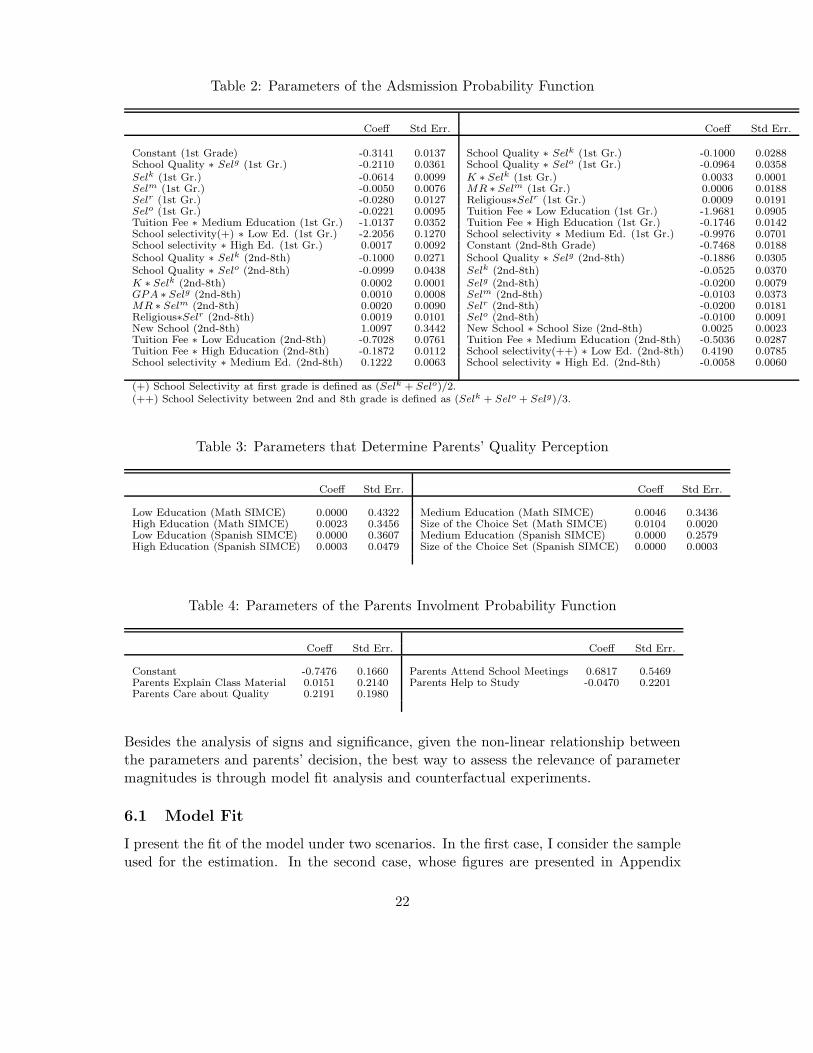
Table 2: Parameters of the Adsmission Probability Function

Coeff Std Err. Coeff Std Err.

Constant (1st Grade) -0.3141 0.0137 School Quality ∗ Selk (1st Gr.) -0.1000 0.0288School Quality ∗ Selg (1st Gr.) -0.2110 0.0361 School Quality ∗ Selo (1st Gr.) -0.0964 0.0358Selk (1st Gr.) -0.0614 0.0099 K ∗ Selk (1st Gr.) 0.0033 0.0001Selm (1st Gr.) -0.0050 0.0076 MR ∗ Selm (1st Gr.) 0.0006 0.0188Selr (1st Gr.) -0.0280 0.0127 Religious∗Selr (1st Gr.) 0.0009 0.0191Selo (1st Gr.) -0.0221 0.0095 Tuition Fee ∗ Low Education (1st Gr.) -1.9681 0.0905Tuition Fee ∗ Medium Education (1st Gr.) -1.0137 0.0352 Tuition Fee ∗ High Education (1st Gr.) -0.1746 0.0142School selectivity(+) ∗ Low Ed. (1st Gr.) -2.2056 0.1270 School selectivity ∗ Medium Ed. (1st Gr.) -0.9976 0.0701School selectivity ∗ High Ed. (1st Gr.) 0.0017 0.0092 Constant (2nd-8th Grade) -0.7468 0.0188School Quality ∗ Selk (2nd-8th) -0.1000 0.0271 School Quality ∗ Selg (2nd-8th) -0.1886 0.0305School Quality ∗ Selo (2nd-8th) -0.0999 0.0438 Selk (2nd-8th) -0.0525 0.0370K ∗ Selk (2nd-8th) 0.0002 0.0001 Selg (2nd-8th) -0.0200 0.0079GPA ∗ Selg (2nd-8th) 0.0010 0.0008 Selm (2nd-8th) -0.0103 0.0373MR ∗ Selm (2nd-8th) 0.0020 0.0090 Selr (2nd-8th) -0.0200 0.0181Religious∗Selr (2nd-8th) 0.0019 0.0101 Selo (2nd-8th) -0.0100 0.0091New School (2nd-8th) 1.0097 0.3442 New School ∗ School Size (2nd-8th) 0.0025 0.0023Tuition Fee ∗ Low Education (2nd-8th) -0.7028 0.0761 Tuition Fee ∗ Medium Education (2nd-8th) -0.5036 0.0287Tuition Fee ∗ High Education (2nd-8th) -0.1872 0.0112 School selectivity(++) ∗ Low Ed. (2nd-8th) 0.4190 0.0785School selectivity ∗ Medium Ed. (2nd-8th) 0.1222 0.0063 School selectivity ∗ High Ed. (2nd-8th) -0.0058 0.0060

(+) School Selectivity at first grade is defined as (Selk + Selo)/2.(++) School Selectivity between 2nd and 8th grade is defined as (Selk + Selo + Selg)/3.

Table 3: Parameters that Determine Parents’ Quality Perception

Coeff Std Err. Coeff Std Err.

Low Education (Math SIMCE) 0.0000 0.4322 Medium Education (Math SIMCE) 0.0046 0.3436High Education (Math SIMCE) 0.0023 0.3456 Size of the Choice Set (Math SIMCE) 0.0104 0.0020Low Education (Spanish SIMCE) 0.0000 0.3607 Medium Education (Spanish SIMCE) 0.0000 0.2579High Education (Spanish SIMCE) 0.0003 0.0479 Size of the Choice Set (Spanish SIMCE) 0.0000 0.0003

Table 4: Parameters of the Parents Involment Probability Function

Coeff Std Err. Coeff Std Err.

Constant -0.7476 0.1660 Parents Attend School Meetings 0.6817 0.5469Parents Explain Class Material 0.0151 0.2140 Parents Help to Study -0.0470 0.2201Parents Care about Quality 0.2191 0.1980

Besides the analysis of signs and significance, given the non-linear relationship betweenthe parameters and parents’ decision, the best way to assess the relevance of parametermagnitudes is through model fit analysis and counterfactual experiments.

6.1 Model Fit

I present the fit of the model under two scenarios. In the first case, I consider the sampleused for the estimation. In the second case, whose figures are presented in Appendix

22

C.1, I use the complete sample (all the students in Santiago City).55 I discuss the fit ofthe model under these two scenarios, since these are also the two samples that I considerin the counterfactual experiments, and because showing that the fit is similar in thetwo cases reinforces the point that the model is capturing the main mechanisms thatdetermine parent decision, without overfitting the data.

As Figure 1 shows, the simulation of the model overall fits the pattern of the studentswho switch school by grade. However, the model has difficulty in generating the increasein school switching that occurs at the end of 6th grade. This increase is mainly drivenby the entry of new public schools in 7th grade (for the new cycle), something that themodel can only partially generate. Moreover, as Figure 2 shows, the model does a goodjob of predicting the 8-year total school changes, by parents’ education.56

Figure 1: Fraction of students changing their school by grade

2nd 3th 4th 5th 6th 7th 8th0

0.01

0.02

0.03

0.04

0.05

0.06

0.07

0.08

Grade

DataSimulation

55In Appendix A, Table 11 shows descriptive statistics for these two samples.56In the estimation and in the simulation, I collapse the information of parents’ education into three

categories: (1) both parents did not complete secondary education (low education); (2) One of the parentscompleted secondary education, but both parents did not attend higher education (medium education);and (3) at least one of the parents attended higher education (high education).

23

Figure 2: Average total change by parents’ education

Low Medium High0

0.1

0.2

0.3

0.4

0.5

Parents education

DataSimulation

Given the kind of counterfactual experiments that I perform, it is relevant to assesshow the model fits the data with regard to some patterns of the decision of parents.For instance, Figure3 shows how the model fits parents’ choice in terms of school type,namely, their decision about attending public, voucher-private or non voucher-privateschools.

Figure 3: Student fraction by school type

Public Private−Voucher Private−Non Voucher0

0.1

0.2

0.3

0.4

0.5

0.6

0.7

School type

DataSimulation

One common feature of many educational systems, which is extremely problematic in

24

the Chilean case,57 is the fact that students’ access to different schools in terms ofquality depends on their income. In the context of the model, this means that the initialknowledge gap K0i − K0i′ , is increased by KT i − KT i′ − (K0i −K0i′) = (KT i −K0i) −(KT i′ −K0i′).

The model has several channels that can generate this correlation: parents can havedifferences in preferences about quality, differences in cognitive skills to understand in-formation about schools, differences in involvement in the child’s school, and differencesin their choice restrictions. Figure 4 shows how, in the data and in the model, the knowl-edge gain is positively correlated with parents’ education. This figure also says that themodel overpredicts the gain for students with parents of low or medium education, andunderpredicts this gain for students with highly educated parents.

Figure 4: Gain in Knowledge by parents education (KT −K0)

Low Medium High−0.8

−0.6

−0.4

−0.2

0

0.2

0.4

0.6

Parents education

std

DataSimulation

Overall, the fit of the model when the sample considers all the students in Santiago Cityis similar to the model fit when the estimation sample is used (Appendix C.1). The mostimportant difference is that the former underestimates the frequency of school switches.

6.2 Parents Perception about Quality

Given the estimated parameters, it is possible to calculate the differences between par-ents’ perception about school quality (which is determined by ηi) and the effective qualityof each school (qjt, i.e., the schools’ fixed effects of test score regressions). Moreover, itis interesting to see how the distance between perception and reality affects the threeschool types differently.

57Valenzuela et al. (2014).

25

To this end, I take two prototypical parents, both of the same educational level, but onewith a small choice set (20 schools), the other with a big choice set (100 schools),58 andthen calculate which would be their quality perception for each school of the sample.To conclude, I calculate the distance between perception and reality for each school.59

Figure 5 shows the results of this exercise. In the first place, there is an importantdistance between perception and reality. In the second place, this misperception is lesssevere for parents facing an smaller choice set. Finally, this misperception biases parents’preferences toward private schools. This bias is driven by the fact that voucher-privateschools have more educated parents than public schools, whereas the same is true betweennon voucher-private and voucher-private schools. As discussed in the model section,because ηiχ ≥ 0, parents overestimate the quality for schools whose students have, onaverage, highly educated parents.

Figure 5: Quality misperception by school administration type (2004)

(a) Parents with small choice set (S(Λ) = 20)

−0.2 −0.1 0 0.1 0.2 0.30

5

10

15

20

25

Den

sity

Perception about quality − Real quality (std)

PublicVoucher−PrivateNon voucher−Private

(b) Parents with big choice set (S(Λ = 100))

−0.5 0 0.5 10

1

2

3

4

5

6

Den

sity

Perception about quality − Real quality (std)

PublicVoucher−PrivateNon voucher−Private

6.3 Counterfactual Experiments

To assess how important school quality is in parents’ decisions, I simulate the model,randomly picking half of the schools and increasing their quality by 0.5 std, while de-creasing the quality of the rest by the same amount. Then, I calculate the increase inthe fraction of parents sending their children to the former schools. To see how relevantquality is in the first decision (first grade), vis-a-vis later decisions, I do this exerciseby increasing schools’ quality in different periods. For instance, I do not affect schoolquality until t, and I perform these quality changes from t+ 1 to T .

Figure 6 shows the results of these exercises. On one hand, there is a moderate increase,of 8-10 percentage points, in the demand for schools that increase their quality since the

58As can be seen from Figure 7, a choice set of 100 schools is not an outlier.59In practice, what I calculate is Et−1[qjt|Dit−1 6= j]− qjt.

26

first period. On the other hand, the effect is irrelevant when schools change their qualityafter the first decision is made (1st grade). These results highlight the relevance of theestimated switching cost.

Figure 6: Increase in the fraction of students in schools with higher quality

1st 2nd 3th 4th 5th 6th 7th 8th−2

0

2

4

6

8

10

12

Grade

diffe

renc

e in

per

cent

age

poin

ts

200420052006200720082009

To study the mechanisms in parents’ demand that explain the frequency of switchingschools, the allocation of students across school types, and the correlation between thegain in knowledge and parents’ educational level, I simulate the model under the followingscenarios:60

• Scenario (1): There is no misperception (η = 0), thus parents correctly estimateschool quality from standardized tests.

• Scenario (2): Parents only cares about quality, which means that U = β ∗K +C ∗ (Dit 6= Dit−1) + ǫ.

• Scenario (3): All students are admitted, thus P (ADitj = 1|Xi) = 1 ∀i, j, t.

• Scenario (4): There is a random admissions process, i.e., ADij ⊥⊥ Xi.

• Scenario (5): the cost of changing school is reduced by 10% (C ∗ 0.9).

60It should be noticed that many of these policies may affect the choice set definition. Thus, giventhat a choice set is fixed in all these simulations, the effects of these policies are underestimated in thisanalysis.

27

• Scenario (6): Parents with the lowest education are relocated to the municipalitywith highest average quality. Parents with the highest education are relocated tothe municipality with lowest average quality.

• Scenario (7): All the students have the same knowledge endowment (K0). Inparticular, EDi = 3 ∀i.

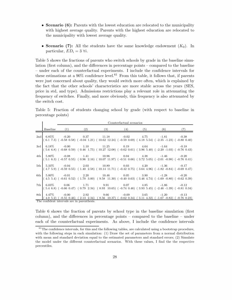
Table 5 shows the fractions of parents who switch schools by grade in the baseline simu-lation (first column), and the differences in percentage points – compared to the baseline– under each of the counterfactual experiments. I include the confidence intervals forthese estimations at a 90% confidence level.61 From this table, it follows that, if parentswere just concerned about quality, they would switch more often, which is explained bythe fact that the other schools’ characteristics are more stable across the years (SES,price in std, and type). Admissions restrictions play a relevant role in attenuating thefrequency of switches. Finally, and more obviously, this frequency is also attenuated bythe switch cost.

Table 5: Fraction of students changing school by grade (with respect to baseline inpercentage points)

Counterfactual scenarios

Baseline (1) (2) (3) (4) (5) (6) (7)

2nd 6.85% -0.20 0.37 11.18 -0.02 4.75 -1.81 -0.38( 6.1 7.3) ( -0.58 0.58) ( -0.04 1.21) ( 10.62 12.24) ( -0.59 0.69) ( 4.18 5.54) ( -2.35 -1.23) ( -0.80 0.40)

3rd 6.18% -0.00 1.10 11.25 0.19 4.64 -1.64 -0.18( 5.6 6.8) ( -0.68 0.59) ( 0.46 1.75) ( 10.27 12.08) ( -0.62 0.61) ( 3.96 5.40) ( -2.20 -1.03) ( -0.76 0.43)

4th 5.80% -0.08 1.41 10.96 0.04 4.38 -1.46 -0.20( 5.1 6.3) ( -0.57 0.55) ( 0.96 2.16) ( 10.07 11.97) ( -0.51 0.66) ( 3.72 5.05) ( -2.01 -0.98) ( -0.76 0.41)

5th 5.33% -0.04 2.03 10.89 0.03 4.20 -1.36 -0.17( 4.7 5.9) ( -0.59 0.55) ( 1.40 2.58) ( 10.14 11.71) ( -0.42 0.75) ( 3.64 4.96) ( -1.82 -0.84) ( -0.69 0.47)

6th 5.00% -0.01 2.20 10.46 0.05 3.90 -1.28 -0.20( 4.5 5.4) ( -0.61 0.52) ( 1.70 3.00) ( 9.58 11.30) ( -0.40 0.63) ( 3.46 4.74) ( -1.69 -0.80) ( -0.62 0.39)

7th 6.03% 0.06 1.71 9.91 0.07 4.85 -1.86 -0.12( 5.4 6.8) ( -0.66 0.47) ( 0.79 2.34) ( 8.93 10.65) ( -0.74 0.46) ( 3.93 5.45) ( -2.46 -1.39) ( -0.81 0.34)

8th 4.47% -0.00 2.92 9.66 -0.09 3.65 -1.20 -0.13( 4.0 5.2) ( -0.55 0.46) ( 2.13 2.34) ( 8.56 10.37) ( -0.62 0.34) ( 3.11 4.32) ( -1.67 -0.82) ( -0.76 0.23)

The confident intervals are in parenthesis.

Table 6 shows the fraction of parents by school type in the baseline simulation (firstcolumn), and the differences in percentage points – compared to the baseline – undereach of the counterfactual experiments. As above, I include the confidence intervals

61The confidence intervals, for this and the following tables, are calculated using a bootstrap procedure,with the following steps in each simulation: (1) Draw the set of parameters from a normal distributionwith mean and standard deviation equal to the estimated parameters and standard errors; (2) Simulatethe model under the different counterfactual scenarios. With these values, I find the the respectivepercentiles.

28

for these estimations at a 90% confidence level. Even though parents’ perception isimportantly biased in favor of private schools (with and without vouchers), when theydecide based on the real quality, the fraction of parents attending public schools increasesby a moderate 1.2 percentage points (with the confidence interval including 0). This smalleffect, relative to the size of the misperception, is explained by the fact that parents donot care too much about quality. In fact, if parents were only concerned with schoolquality, there would be an increase of 2.6 percentage points in the fraction of parentschoosing public schools, while this figure would decrease by 3.4 percentage points forvoucher-private schools. This basically reflects the fact that the other elements of theutility function (SES of the school, the preference for its type, etc.) lead parents to applyto private schools.62 Finally, these simulations allow us to see what would happen if lesseducated parents had a more relaxed choice set constraint. Scenarios 3, 4, and 7, all tellthe same story: less choice set restrictions would lead (less educated) parents to chooseprivate schools more often, though not necessary because of their higher quality.

Table 6: Student fraction by school type at first grade (with respect to baseline inpercentage points)

Counterfactual scenarios

Baseline (1) (2) (3) (4) (5) (6) (7)

Public 29.26% 1.20 2.60 -2.87 -2.99 0.71 0.45 -3.39( 26.6 31.7) ( -0.37 2.00) ( -0.02 4.98) ( -4.11 -1.84) ( -4.30 -2.13) ( -0.46 1.91) ( -1.27 1.05) ( -5.02 -2.37)

Voucher 65.35% -0.76 -3.44 -0.29 -0.26 -0.76 2.53 1.96Private ( 62.2 68.1) ( -1.61 0.85) ( -6.06 -0.47) ( -1.38 1.05) ( -1.15 1.28) ( -2.00 0.63) ( 1.68 4.35) ( 0.67 3.30)

Non voucher 5.38% -0.44 0.84 3.16 3.25 0.05 -2.98 1.44Private ( 4.0 7.0) ( -1.14 0.12) ( -1.07 2.15) ( 2.45 3.75) ( 2.12 4.08) ( -0.73 0.42) ( -3.96 -2.13) ( 0.91 2.32)

Table 7 shows the knowledge that students gained between 2004 and 2011, by parents’education. In addition, in the last row I present the change in the overall quality. Again,I include the confidence intervals for these estimations at a 90% confidence level. Whilethe numbers of the baseline simulation are presented in the first column, the numbers inthe other columns are the differences in standard deviations – compared to the baseline –under each of the counterfactual experiments. The first result to notice is that, while anexclusive focus on quality would increase the knowledge gained by students whose parentshave medium or high education, this shift in preferences would not have a relevant effectfor students whose parents have a low level of education. This confirms the relevanceof choice restrictions: for some parents, even if they put more weight on quality, theycannot find a better school for their child. A second element to notice is that bothprohibiting schools from making admission decisions based on student characteristics and

62It should be noticed that, in this model, peer effects are part of the school quality, which is constantin all the policy experiments. Therefore, in this model it is not possible to study a potential self-fulfillingprophecy, in which parents think that private schools are better, and therefore apply to those schools;those schools select the best students (those who have more educated parents); and, because of thatpattern of admissions decisions, and given the peer effect, private schools end up being better than thepublic ones.

29

reallocating the poor families to better municipalities are effective measures to reducethe gap between students with parents with different levels of education.63

Table 7: Gain of knowledge (KT −K0) by parents education (with respect to baselinein standard deviations).

Counterfactual scenarios

Baseline (1) (2) (3) (4) (5) (6) (7)

Incompleted High -52.79% 0.00 0.03 0.10 0.08 0.00 -0.09 0.10School ( -61.1 -43.1) ( -0.07 0.04) ( -0.07 0.11) ( 0.04 0.16) ( 0.02 0.13) ( -0.05 0.04) ( -0.14 -0.03) ( 0.05 0.17)

Completed High -27.32% -0.02 0.08 0.14 0.11 0.00 -0.00 0.12School ( -35.2 -18.5) ( -0.07 0.02) ( 0.00 0.16) ( 0.09 0.18) ( 0.07 0.16) ( -0.03 0.03) ( -0.03 0.03) ( 0.07 0.17)

With college 18.76% -0.06 0.17 0.09 0.05 0.00 0.08 0.00Studies ( 7.4 31.2) ( -0.11 -0.00) ( 0.06 0.27) ( 0.04 0.13) ( 0.00 0.09) ( -0.05 0.03) ( 0.00 0.16) ( -0.04 0.04)

All -15.90% -0.03 0.10 0.12 0.08 0.00 0.01 0.07( -23.1 -7.0) ( -0.07 -0.01) ( 0.03 0.16) ( 0.08 0.14) ( 0.05 0.11) ( -0.03 0.02) ( -0.02 0.04) ( 0.04 0.10)

Finally, regarding the gain in the overall quality, as expected, an exclusive focus onquality increases the gain in quality. If the parents have a more relaxed choice setconstraint, there is an increase in such a gain. Surprisingly, if parents have no qualitymisperception, there is a small decrease in the overall gain in quality. This is due tothe fact that when parents exaggerate the quality of some schools due to misperception,implicitly they also care more about school quality relative to other characteristics ofthe schools, which leads parents to choose better schools in terms of quality. In otherwords, parents’ misperception generates two distortions. On the one hand, parents failto properly assess the real ranking of schools in terms of quality. This effect decreasesthe overall gain in quality. On the other hand, there is a change in school’ qualitydistribution, which is equivalent to a change in the weights that parents place on schoolquality in their utility function. The latter effect could decrease or increase the overallgain in quality. However, in this case, it increases it.

Appendix C.2 contains the tables that show the results of the counterfactual experimentswhen using the complete sample, which includes all the students of Santiago City whoentered first grade in 2003. Although the complete sample incorporates all the small mu-nicipalities that were not part of the estimation sample, the main conclusions (elaboratedfrom Tables 5, 6, and 7) are not affected.

63This can be concluded by looking at columns 5, 8, and 7 of Table 7. Notice that in all thesecounterfactual experiments, the choice set (Λ) is fixed, in the sense that the set is invariant conditionalon the municipality where parents live and their educational level. Thus, when a family of parents withlow education is relocated from municipality A to municipality B, their new choice set (Λ) is going bethe choice set of a family with low-educated parents who live in municipality B.

30

7 Conclusions

This paper estimates a dynamic model of elementary school choice. To this end, Iuse detailed Chilean administrative data for the students who entered 1st grade of theelementary cycle in 2003, following them until 8th grade (2011), which in Chile is theend of the elementary cycle. The estimated model considers several elements that arerelevant to explain parents’ decisions, namely, how much do they care about schoolquality (and other school characteristics), parents’ skill in understanding informationabout quality (national standardized tests), parents’ involvement in the school attendedby their children, and their choice set.

Assessing the relevance of these different components contributes to a better understand-ing of the demand for schools and the role that markets with competitive incentives canhave in education. In particular, the structural approach followed in this paper allows meto quantify different sources of unequal access to high quality schools and of the higher de-mand for private schools than for public schools. In doing so, this paper also contributesto the scarce literature that estimates structural models with bounded rationality, aswell as to the literature which uses observed choices to infer agents’ information.

Regarding the debate about the extent to which parents base their decisions on schoolquality, I find that parents do care about school quality, but only to a moderate degree.Moreover, the simulations show that parents’ decisions are not sensitive to changes inquality after the first decision (1st grade). I also find that more involved parents caremarginally more about school quality.

The results show that parents have an important misperception about school quality,which causes them to have a less favorable opinion about public schools, relative toprivate schools. This result supports the idea that parents may have difficulty in isolatinga school’s quality from its socioeconomic composition when they observe test scores.However, given that quality is not very relevant for their decision, such a misperceptionhas only a limited effect on parents’ decisions.

Concerning the question of why parents choose private schools over public schools, theresults show that, if parents were only concerned about quality, they would choose publicschools more often. The result would be the same if they did not have a misperceptionabout quality. However, if parents had more freedom in terms of the schools their childrencould attend, they would choose private schools more often. This last result suggeststhat admission rules are binding restrictions and that relaxing them would increase thedemand for private schools.

Regarding the causes of the increase in the knowledge gap between students from dif-ferent socioeconomic backgrounds, simulations show that schools’ admission rules andhousehold location are relevant in explaining the rise in this gap. This result supportsthe papers which argue that Chilean SES school segregation cannot be explained onlyby geographical segregation.64

64See, for example, Valenzuela et al. (2014), Elacqua (2012) and Hsieh and Urquiola (2006).

31

Finally, it should be noticed that, even though these counterfactual exercises are veryuseful to compare the effects of different policies on relevant outcomes (e.g., inequality),these are in general small effects. The latter can be partially explained by the fact that,in all the simulations, the choice set is fixed conditional on parents’ education and homelocation. This limitation is something that should be addressed in future research.

32

References

Aguirregabiria, V. and P. Mira (2010). Dynamic discrete choice structural models: Asurvey. Journal of Econometrics 156 (1), 38 – 67. Structural Models of OptimizationBehavior in Labor, Aging, and Health.

Alderman, H., P. F. Orazem, and E. M. Paterno (2001). School quality, school cost, andthe public/private school choices of low-income households in pakistan. The Journalof Human Resources 36 (2), pp. 304–326.

Angrist, J., E. Bettinger, and M. Kremer (2006). Long-term educational consequences ofsecondary school vouchers: Evidence from administrative records in colombia. Amer-ican Economic Review 96 (3), 847–862.

Auguste, S. and J. P. Valenzuela (2006). Is it just cream skimming? school vouchers inchile. Technical report.

Azmat, G. and J. Garcia-Montalvo (2012, June). The role of awareness, informationgathering and processing in school choice. Working Papers 639, Barcelona GraduateSchool of Economics.

Bast, J. L. and H. J. Walberg (2004). Can parents choose the best schools for theirchildren? Economics of Education Review 23 (4), 431 – 440. Special Issue In Honorof Lewis C. Solman.

Bellei, C. (2009). The private-public school controversy: The case of chile. In P. Petersonand R. Chakrabarti (Eds.), School Choice International, pp. 165–192. Cambridge, MA:MIT Press.

Bettinger, E. (2011). Chapter 7 - educational vouchers in international contexts. InS. M. Eric A. Hanushek and L. Woessmann (Eds.), Handbook of The Economics ofEducation, Volume 4 of Handbook of the Economics of Education, pp. 551 – 572.Elsevier.

Black, S. E. (1999). Do better schools matter? parental valuation of elementary educa-tion. The Quarterly Journal of Economics 114 (2), 577–599.

Bravo, D., S. Mukhopadhyay, and P. E. Todd (2010). Effects of school reform on educa-tion and labor market performance: Evidence from chile’s universal voucher system.Quantitative Economics 1 (1), 47–95.

Carneiro, P., K. T. Hansen, and J. J. Heckman (2003). 2001 lawrence r. klein lecture:Estimating distributions of treatment effects with an application to the returns toschooling and measurement of the effects of uncertainty on college choice. InternationalEconomic Review 44 (2), pp. 361–422.

Chumacero, R. A., D. Gomez, and R. D. Paredes (2011, October). I would walk 500 miles(if it paid): Vouchers and school choice in chile. Economics of Education Review 30 (5),1103–1114.

33

Conlisk, J. (1996). Why bounded rationality? Journal of Economic Literature 34 (2),669–700.

Contreras, D., P. Sepulveda, and S. Bustos (2010). When schools are the ones thatchoose: The effects of screening in chile. Social Science Quarterly 91 (s1), 1349–1368.

Cunha, F., J. Heckman, and S. Navarro (2005, April). Separating uncertainty fromheterogeneity in life cycle earnings. Oxford Economic Papers 57 (2), 191–261.

Drago, J. L. and R. Paredes (2011). La brecha de calidad en la educacion chilena. CepalReview 104, 167–180.

Eckstein, Z. and K. I. Wolpin (1989). The specification and estimation of dynamicstochastic discrete choice models: A survey. The Journal of Human Resources 24 (4),pp. 562–598.

Elacqua, G. (2012). The impact of school choice and public policy on segregation: Ev-idence from chile. International Journal of Educational Development 32 (3), 444 –453.

Epple, D. and R. Romano (2008). Educational vouchers and cream skimming. Interna-tional Economic Review 49 (4), 1395–1435.

Epple, D. and R. Romano (2012, 07). Economic modeling and analysis of educationalvouchers. Annual Review of Economics 4 (1), 159–183.

Epple, D. and R. E. Romano (1998). Competition between private and public schools,vouchers, and peer-group effects. The American Economic Review 88 (1), pp. 33–62.

Gallego, F. A. and A. E. Hernando (2008). On the determinants and implications ofschool choice: Semi-structural simulations for chile [with comments]. Economıa 9 (1),pp. 197–244.

Gauri, V. (1999). School Choice In Chile: Two Decades of Educational Refor. Pitt LatinAmerican Studies. University of Pittsburgh Press.

Geyer, J. and H. Sieg (2013, November). Estimating a model of excess demand for publichousing. Quantitative Economics 4 (3), 483–513.

Hanushek, E. A., J. F. Kain, and S. G. Rivkin (2004). Disruption versus tieboutimprovement: the costs and benefits of switching schools. Journal of Public Eco-nomics 88 (9?10), 1721 – 1746.

Hastings, J. S. and J. M. Weinstein (2008, November). Information, school choice, andacademic achievement: Evidence from two experiments. The Quarterly Journal ofEconomics 123 (4), 1373–1414.

34

Henig, J. (1996). The local dynamics of choice: Ethnic preferences and institutionalresponses. In R. E. B. Fuller and G. Orfield (Eds.), Who chooses? Who loses? Culture,institutions, and the unequal effects of school choice, pp. 93–117. New York: TeachersCollege Press.

Houser, D., M. Keane, and K. McCabe (2004). Behavior in a dynamic decision problem:An analysis of experimental evidence using a bayesian type classification algorithm.Econometrica 72 (3), 781–822.

Hsieh, C.-T. and M. Urquiola (2006, September). The effects of generalized school choiceon achievement and stratification: Evidence from chile’s voucher program. Journal ofPublic Economics 90 (8-9), 1477–1503.

Kane, T. J., S. K. Riegg, and D. O. Staiger (2006). School quality, neighborhoods, andhousing prices. American Law and Economics Review 8 (2), 183–212.

Keane, M. P. and K. I. Wolpin (1994, November). The solution and estimation ofdiscrete choice dynamic programming models by simulation and interpolation: Montecarlo evidence. The Review of Economics and Statistics 76 (4), 648–72.

Larranaga, O. (2004, March). Competencia y participacion privada: La experienciachilena en educacion. Working Papers wp208, University of Chile, Department ofEconomics.

Mark, G. Elacqua, and J. Buckley (2006). School choice in chile: Is it class or theclassroom? Journal of Policy Analysis and Management 25 (3), 577–601.

McMillan, R. (2004). Competition, incentives, and public school productivity. Journalof Public Economics 88 (9?10), 1871 – 1892.

Meckes, L. and R. Carrasco (2010). Two decades of simce: an overview of the nationalassessment system in chile. Assessment in Education: Principles, Policy and Prac-tice 17 (2), 233–248.

Mizala, A. and P. Romaguera (2000). School performance and choice: The chileanexperience. The Journal of Human Resources 35 (2), pp. 392–417.

Mizala, A., P. Romaguera, and M. Urquiola (2007). Socioeconomic status or noise?tradeoffs in the generation of school quality information. Journal of DevelopmentEconomics 84 (1), 61–75.

Mizala, A. and M. Urquiola (2013). School markets: The impact of information ap-proximating schools’ effectiveness. Journal of Development Economics 103 (0), 313 –335.

Navarro, S. (2011). Using observed choices to infer agent’s information: Reconsider-ing the importance of borrowing constraints, uncertainty and preferences in collegeattendance. Technical report.

35

Neilson, C. (2013). Targeted vouchers, competition among schools, and the academicachievement of poor students. Technical report.

Rothstein, J. M. (2006). Good principals or good peers? parental valuation of schoolcharacteristics, tiebout equilibrium, and the incentive effects of competition amongjurisdictions. American Economic Review 96 (4), 1333–1350.

Rust, J. (1994, January). Structural estimation of markov decision processes. In R. F.Engle and D. McFadden (Eds.), Handbook of Econometrics, Volume 4 of Handbook ofEconometrics, Chapter 51, pp. 3081–3143. Elsevier.

Schneider, M., P. Teske, M. Marshall, and C. Roch (1998). Shopping for schools: In theland of the blind, the one-eyed parent may be enough. American Journal of PoliticalScience 42 (3), pp. 769–793.

Simon, H. A. (1986). Rationality in psychology and economics. In R. M. Hogarth andM. W. Reader (Eds.), In Rational Choice: The Contrast Between Economics andPsychology, pp. 25–40. Chicago: University of Chicago Press.

Valenzuela, J. P., C. Bellei, and D. d. l. Rıos (2014). Socioeconomic school segrega-tion in a market-oriented educational system. the case of chile. Journal of EducationPolicy 29 (2), 217–241.

Zamora, G. (2011, 00). Movilidad escolar en Chile: Analisis de las Implicancias para laCalidad y Equidad de la Educacion. Estudios pedagogicos (Valdivia) 37, 53 – 69.

36

A Figures and Tables

Table 8: Descriptive statistics of students with and without grade retention history

Variable Students who did not Students who Difference z-statistic P-Valuerepeat a grade repeated a grade

Changed school at least once 0.50 0.70 -0.201 -67.37 0.00

Moved to another house 0.09 0.12 -0.025 -14.11 0.00

Can not afford the tuition fee 0.03 0.05 -0.020 -19.27 0.00

Forced to switch given low performance 0.01 0.05 -0.041 -63.72 0.00

Students did not like the school 0.06 0.11 -0.054 -35.82 0.00

Parents found better school 0.15 0.10 0.046 22.32 0.00

School does not offer secondary level 0.04 0.04 0.000 0.18 0.86

Another reason 0.11 0.17 -0.063 -32.85 0.00

Number of observations 165606 34327

The sample contains all the students who took 2011 SIMCE for 8th grade.

Table 9: Fraction of students changing school

2nd 3th 4th 5th 6th 7th 8th N

All 0.06 0.06 0.05 0.05 0.05 0.07 0.04 77432

Mother’s education

Incomplete 0.04 0.04 0.04 0.04 0.03 0.04 0.03 6962elementary school

Complete 0.06 0.05 0.04 0.05 0.03 0.05 0.03 8182elementary school

Incomplete 0.06 0.05 0.05 0.05 0.05 0.06 0.04 11085secondary school

Complete 0.06 0.06 0.05 0.05 0.05 0.08 0.04 29667secondary school

Complete or 0.06 0.07 0.06 0.06 0.06 0.09 0.06 21536incomplete college

Note: I drop the students who fail at least one class between 1st and 8th grade,and I also drop the students whose families switch the municipality where theylive.

37

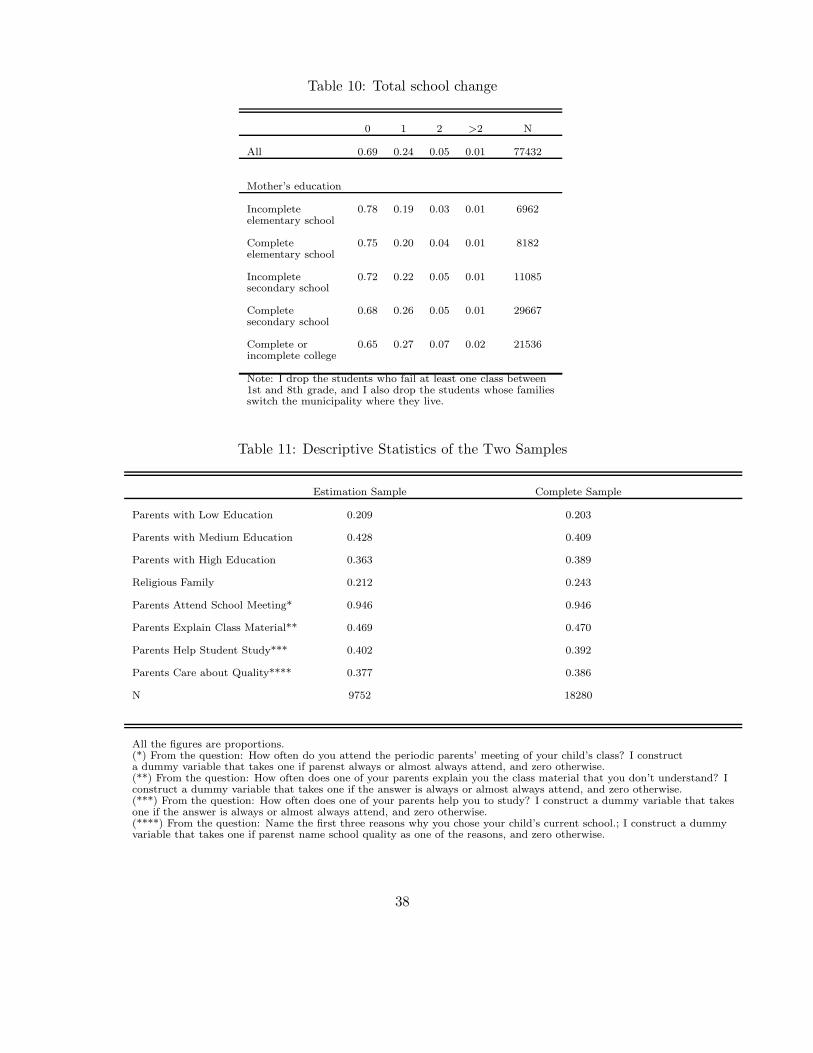
Table 10: Total school change

0 1 2 >2 N

All 0.69 0.24 0.05 0.01 77432

Mother’s education

Incomplete 0.78 0.19 0.03 0.01 6962elementary school

Complete 0.75 0.20 0.04 0.01 8182elementary school

Incomplete 0.72 0.22 0.05 0.01 11085secondary school

Complete 0.68 0.26 0.05 0.01 29667secondary school

Complete or 0.65 0.27 0.07 0.02 21536incomplete college

Note: I drop the students who fail at least one class between1st and 8th grade, and I also drop the students whose familiesswitch the municipality where they live.

Table 11: Descriptive Statistics of the Two Samples

Estimation Sample Complete Sample

Parents with Low Education 0.209 0.203

Parents with Medium Education 0.428 0.409

Parents with High Education 0.363 0.389

Religious Family 0.212 0.243

Parents Attend School Meeting* 0.946 0.946

Parents Explain Class Material** 0.469 0.470

Parents Help Student Study*** 0.402 0.392

Parents Care about Quality**** 0.377 0.386

N 9752 18280

All the figures are proportions.(*) From the question: How often do you attend the periodic parents’ meeting of your child’s class? I constructa dummy variable that takes one if parenst always or almost always attend, and zero otherwise.(**) From the question: How often does one of your parents explain you the class material that you don’t understand? Iconstruct a dummy variable that takes one if the answer is always or almost always attend, and zero otherwise.(***) From the question: How often does one of your parents help you to study? I construct a dummy variable that takesone if the answer is always or almost always attend, and zero otherwise.(****) From the question: Name the first three reasons why you chose your child’s current school.; I construct a dummyvariable that takes one if parenst name school quality as one of the reasons, and zero otherwise.

38

B Estimated Parameters and Model’s Inputs

B.1 Model’s Inputs and Parameters Estimated Outside the Model

Figure 7: Histogram of the Size of the Choice Sets

0 20 40 60 80 100 120 140 160 180 2000

500

1000

1500

2000

2500

Size of the Choice Set

39

Figure 8: Distribution of Estimated Quality by School Type in 2004

−2 −1 0 1 2 3 40

0.5

1

1.5

2

2.5

3

dens

ity

School Quality

PublicVoucher−privateNon voucher−private

40

Figure 9: Distribution of test scores by School Type in 2004

−3 −2 −1 0 1 2 30

0.5

1

1.5

2

dens

ity

Average test scores

PublicVoucher−privateNon voucher−private

??

Table 12: Knowledge Production Function

Coeff Std Err.

Accumulated School Quality at 8th Grade 3.69 0.0314

Parents with Medium Level of Education 5.49 0.2396

Parents with High Level of Education 9.21 0.2646

Constant 256.59 0.1947

N = 55, 421R2 = 0.2113Note: This is the result of estimating the Knowledge Production Function KijT = α0Xi + α1

∑T

t=1 qijt + ϑijT .The omiited dummy variable is Parents with Low Level of Education.

41

Table 13: GPA Production Function

4th 2005 4th 2006 4th 2007 4th 2008 4th 2009 8th 2011

Coeff SE Coeff SE Coeff SE Coeff SE Coeff SE Coeff SE

Entered in 2nd -0.07 0.0034 -0.06 0.0034 -0.06 0.0038 -0.06 0.0039 -0.07 0.0034 -0.05 0.0054

Entered in 3th -0.08 0.0033 -0.08 0.0033 -0.08 0.0036 -0.07 0.0038 -0.07 0.0033 -0.04 0.0050

Entered in 4th -0.11 0.0030 -0.11 0.0030 -0.12 0.0035 -0.10 0.0037 -0.11 0.0032 -0.06 0.0048

Entered in 5th -0.06 0.0045

Entered in 6th -0.08 0.0045

Entered in 7th -0.10 0.0040

Entered in 8th -0.17 0.0046

Constant 3.63 0.0063 3.72 0.0062 3.74 0.0066 3.75 0.0066 3.72 0.0065 3.02 0.0097

N 214,661 210,177 162,552 169,500 178,685 161,920

Adjusted R-squared .549 .545 .559 .537 .558 .465

Note: This is the result of estimating the GPA production function Gijt = λt0j + λt

1jKijt + λt2TAit + ε

gijt, where I only

present the values for λt2. The omitted dummy variable is Entered in 1st grade.

Figure 10: GPA Standards

(a) 2005 (4th Grade)

0 2 4 6 8 10 12−0.02

−0.015

−0.01

−0.005

0

0.005

0.01

0.015

0.02

Slo

pe

Constant

(b) 2011 (8th Grade)

−8 −6 −4 −2 0 2 4 6 8−0.01

0

0.01

0.02

0.03

0.04

0.05

Slo

pe

Constant

Note: Giving the GPA production function Gijt = λt0j + λt

1jKijt + λt2TAit + ε

gijt; λ0j is the constant and λ0j

the slope.

42

C Model Fit and Counterfactual experiments (completesample)

C.1 Model Fit

Figure 11: Model fit for the complete sample

(a) Fraction of student changing their school bygrade

2nd 3th 4th 5th 6th 7th 8th0

0.01

0.02

0.03

0.04

0.05

0.06

0.07

0.08

Grade

DataSimulation

(b) Average total change by parents education

Low Medium High0

0.1

0.2

0.3

0.4

0.5

Parents education

DataSimulation

(c) Student fraction by school type

Public Private−Voucher Private−Non Voucher0

0.1

0.2

0.3

0.4

0.5

0.6

0.7

School type

DataSimulation

(d) Gain in Knowledge by parents education

Low Medium High−0.6

−0.4

−0.2

0

0.2

0.4

0.6

0.8

Parents education

std

DataSimulation

43

C.2 Counterfactual Experiments

Table 14: Fraction of students changing school by grade (with respect to baseline inpercentage points), complete sample.

Baseline No misperception Only Q All admitted Random C ∗ 0.9 New All ED = 3maters admission locations

2nd 6.2% 0.1 0.6 10.9 0.1 4.6 -1.3 -0.1

3th 5.8% -0.0 1.1 10.8 0.0 4.1 -1.4 -0.1

4th 5.3% -0.0 1.6 10.4 0.0 4.1 -1.2 -0.1

5th 4.9% 0.0 1.9 10.3 0.2 4.0 -1.0 -0.1

6th 4.5% 0.0 2.2 9.9 0.2 3.8 -1.0 -0.1

7th 5.2% -0.0 2.0 9.1 -0.0 4.1 -1.4 -0.2

8th 4.2% -0.0 2.6 8.8 -0.1 3.4 -1.1 -0.2

Table 15: Student fraction by school type at first grade (with respect to baseline inpercentage points), complete sample.

Baseline No misperception Only Q All admitted Random C ∗ 0.9 New All ED = 3maters admission locations

Public 27.7% 0.8 2.7 -2.7 -2.8 0.4 0.7 -3.1

Voucher Private 62.6% -0.3 -3.0 -0.3 -0.3 -0.3 6.6 1.8

Non voucher 9.7% -0.6 0.3 3.0 3.1 -0.1 -7.4 1.3Private

Table 16: Gain of knowledge (KT −K0) by parents education (with respect to baselinein standard deviations), complete sample.

Baseline No misperception Only Q All admitted Random C ∗ 0.9 New All ED = 3maters admission locations

Incompleted High -0.429 -0.002 0.010 0.084 0.059 -0.002 -0.118 0.085school

Completed High -0.233 -0.028 0.038 0.111 0.087 -0.009 -0.004 0.112school

With college 0.386 -0.047 0.137 0.075 0.045 -0.001 -0.129 0.011studies

All -0.032 -0.030 0.071 0.091 0.065 -0.005 -0.076 0.067

44