a dynamic model for the study of gear transmissions · a dynamic model for the study of gear ......

A dynamic model for the study of gear transmissions

A. Fernandez del Rincon, F. Viadero, R. Sancibrian, P. Garcia Fernandez & A. de Juan Dept. Structural and Mechanical Engineering, University of Cantabria, Santander, Spain

Abstract

In this work a previous model developed by the authors for the quasi-static analysis of spur gear transmissions supported by ball bearings was modified extending its capabilities to dynamic analysis. The model combines a finite element and an analytical formulation achieving sufficient accuracy and computational efficiency to make dynamic analysis feasible. Non-linearity associated with the contact among teeth was included, taking into account the flexibility of gears, shafts and bearings. Furthermore, parametric excitations originating both from gear and bearing supports, as well as clearance, were also taken into account. An example of a simple transmission is presented providing several results obtained using the proposed model. Nevertheless, in spite of its usefulness, particularly in the case of variable torque loads, and its improved capabilities compared with other procedures, this approach still requires a high computational effort. As a consequence in those cases where the transmission operates under stationary conditions the formulation could be simplified by using a pre-calculated value for each the gear tooth stiffness as a function of the angular position. Once again, the original model is useful, taking advantage of its computational efficiency in the calculation of these stiffness coefficients throughout a meshing period. The improved model is applied to the same transmission and the consequences of a misleading calculation of the stiffness coefficients are shown. Then, it was used to study the vibratory behaviour under different levels of applied torque, showing the modifications suffered by the orbits, meshing contact forces and particularly the spectra obtained for bearing forces. Keywords: gear dynamics, transmission error, bearings, tooth contact.

Computational Methods and Experimental Measurements XIV 523

© 2009 WIT PressWIT Transactions on Modelling and Simulation, Vol 48, www.witpress.com, ISSN 1743-355X (on-line) doi:10.2495/CMEM090471

1 Introduction

The increase in the demands for more efficient and reliable gear transmissions, with higher levels of torque and speed, gives rise to an emergent interest in the development of analytical tools to provide a deeper understanding of dynamics of gear transmissions. This kind of tools could be applied in the improvement of the dynamic performance to reduce the level of noise and vibration, but they also serve as an excellent support for developing new techniques of detection and prediction in the field of condition monitoring based on vibratory measurements. This kind of techniques requires the set up of a condition monitoring system that is normally based on field measurements in order to define the normal vibratory behaviour. Therefore, the development of more accurate models for gear dynamics could serve as a basis for future improvements in this technique and could also increase the capabilities for prediction of the progress of a certain fault. There are a huge number of publications related to the dynamics of gear transmissions. A good revision of the works, as well an interesting introduction to the problems involved in this kind of elements was provided by Ozguven and Houser [1]. The main phenomena involved in gear dynamics are the parametric excitation due the variable number of meshing teeth as well as the non linearity present as a consequence of the backslash. In this sense Kahraman and Singh [2] propose the classification of dynamic gear models as: Linear Time Invariant (LTI), Linear Time Variant (LTV), Non Linear Time Invariant (NLTI) and Non Linear Time Variant (NLTV) depending on the procedure followed in order to include or not these features. In summary, the most important aspect in order to formulate a good dynamic model for gear transmission is the procedure followed to include the meshing contact forces. Nevertheless, there are other components in gear transmissions that present the same kind of dynamic phenomena described for gears. These components are bearings. Bearings behave in a similar way to gears. They also have a parametric excitation due the variable number of roller elements transmitting the load to the supports. However, they also present non linearity as a consequence of the Hertzian contact and clearance [3]. It is clear from the point of view of condition monitoring that both elements should work together and the features of both elements are added in order to give the final vibration signature of the transmission. Therefore, condition monitoring requires the development of dynamic models that provide an accurate description of the dynamic forces as opposed to the most general models, where the interest is mainly focused on the determination of the resonances for design purposes. That means, accurate models for gear dynamics that should include both, gears and bearings in the formulation, taking into account the parametric excitation and non linearity originating from each element. Pursuing this objective, a quasi-static model including those features was presented by the authors in a previous work [4]. The procedure for gear contact force calculation employs a hybrid approach dividing the elastic deflections in teeth into two different contributions: global deflections including bending, and

524 Computational Methods and Experimental Measurements XIV

© 2009 WIT PressWIT Transactions on Modelling and Simulation, Vol 48, www.witpress.com, ISSN 1743-355X (on-line)

Shaft 1

Shaft 2

50 mm 50 mm 50 mm

Ø=40 mm

b11 b12

b21 b22

J22

R11

R21 Input

Ω (constant)

Output Torque

shearing and local deflections in the vicinity of theoretical contact points. Global deflections were obtained by means a plane strain (or plane stress) finite element model taking into account the elastic coupling between successive teeth under a load. Instead, local deflections were approached by a non-linear formulation derived by Weber-Banashek for bi-dimensional problems. Bearings were also included taking into account the clearance, contact non linearity and variation in the number of loaded rolling elements. In this case, a bi-dimensional model was developed where only deflections of Hertzian type are considered, neglecting bending and shearing of races and rolling elements. This model was subsequently used for simulation of several kinds of defects in gears [5]. In this paper, this model was further extended to carry out dynamic calculations. The usefulness is proved by the simulation of the vibratory behaviour of a simple transmission. A faster solution was achieved by the calculation of the meshing stiffness for a certain torque applied to the transmission. This procedure is compared with the original one and the consequences of an inaccurate estimation of the meshing stiffness are analysed. Special attention was given to the resulting spectra as the load condition is modified. That is one of the main drawbacks of introducing and setting up condition monitoring systems in machinery working under variable conditions of load (wind turbines, rolling mills, etc.). Different load levels provide different behaviour and as a consequence the alarm levels should be adapted on the basis of experimental measurements. Thus a good model used during the design task could be a very profitable tool to extend the life of the transmission.

2 Model description

A simple transmission was analysed, as is shown in the schema in fig. 1. This transmission is composed of a couple of twin spur gears mounted on elastic shafts that are supported by two ball bearings. Inertia is lumped at the centre of each element (gear or bearing) allowing translational and rotational movement in the plane. An additional rotational-only inertia is included at the output and a constant value of rotational speed is assumed at the input. That means a dynamic model with 19 degrees of freedom (dof).

Figure 1: Schema and dimensions of a simple transmission.



Following the procedure described in [4], gear contacting forces are obtained based of the model proposed by Andersson and Vedmar [6], where tooth deformations are divided into two groups; one near the contact that is treated by an analytical non-linear formulation of Hertzian type, and another of elastic nature determined by means of a dedicated finite element model. This kind of formulation achieves an efficient treatment of gear teeth contacts, not requiring a highly refined mesh at the contact surfaces. As a consequence the computational effort is reduced compared with conventional finite element models allowing the analysis of dynamic problems. Contact forces in the line of action (LOA) were further improved by the inclusion of friction and damping. Friction forces were added assuming a Coulomb model with constant friction coefficient, taking into account the reversing sense of this force when the contact takes place in the vicinity of the primitive point. In order to avoid numerical problems, a smoothing formulation based on the hyperbolic tangent function was considered according to the following expression

( ) ( ) ( )(1/ 2) 1 (1 / 2)

11 2 10 (1 / 2)

; ;i i

i

P i P

f i i f fi i iP

v t vF F ftgh t F F

v v

⋅= − ⋅ = −

(1)

Where Ff 1i and Ff 2i are force vectors representing friction forces at the i contact on gear 1 and 2, f is the friction coefficient, Fi is the contact force at the i contact, vPi is the relative velocity between the contacting points on each contact surface and t is a unitary vector defining the common normal of the surfaces and v0 is a threshold level to smooth the transition when the relative velocity is null. Conventional models consider damping as an overall term accounting for all dissipative effects neglecting the oil present between contacts. However, the intermediate layer of oil between two approaching surfaces gives rise to a damping effect known as squeeze film damping. In this model, this phenomenon was the only dissipative source considered for gear damping, neglecting other sources such as the hysteretic damping of contacting surfaces. Following this assumption, the squeeze damping was defined by the following expression

3/ 2

1 2

1 2

112 ;2Am nF b v

hχ χ

πηχ χ

= +

(2)

Where η is the dynamic viscosity, b the gear wide, h the thickness of the lubricant film, χi the curvature radius of the contacting surface i and |vn| the modulus of the relative velocity on the normal of the contacting profiles. Assuming that the oil is present around the contacting teeth, the value of h is defined by the minimum distance between contacting profiles that is obtained knowing the position of each gear. In order to avoid the discontinuity when the lubricant thickness is null, a threshold was defined. As the model considers several potential contact points the damping force is obtained for each one taking into account not only those due the active line of action but also those contacts in the reverse line of action. Regarding bearings, the model proposed in [4] was kept unmodified except for the capability of including waviness and localized defects, which will not be



discussed in this work. Random relative sliding of the rolling elements with respect to the cage was also added bearing in mind the smoothing out of the spectral content due the ball pass frequency. Taking into account torsional and flexural deflection of shafts and the formulations described in the previous paragraphs for gears and bearings, the block diagram shown in fig. 2 is achieved. There, the connection among blocks could be carried out by a linear translational/rotational spring with a viscous damper or by a non linear function. Non linear functions are represented by a double sense arrow (in green for gears and blue for bearings). Meshing force calculation includes normal contact forces, friction and squeeze damping, applying the procedure described previously. Otherwise, bearing damping is added in the block diagram as an equivalent translational viscous damping having the same value for any direction on the plane of movement. The same type of damping was used for connecting shafts.

Figure 2: Block diagram of a simple transmission.

Taking a reference frame, with the z-axis oriented along the shaft centre line, from left to right in fig. 1, and the y-axis defined by the line between gear centres. X and Y are the translational degrees of freedom along the x and y-axis while Θ is the rotational degree of freedom around the z-axis. Subscript T denotes torsional properties, b means bearing and R gear. Following this nomenclature, Xibj means the displacement along the x-axis of bearing j

X1b1 Y1b1 Θ1b1

X1R1Y1R1Θ1R1

X1b2Y1b2Θ1b2

C1b1

KT1J1b1

CT1J1b1

C1b2

K1b1R1

C1b1R1 K1R1b2

C1R1b2

f1b1 f1b2

TOut

ΘIn(t)

KT1R1b2

CT1R1b2 KT1b1R1

CT1b1R1

X2R1Y2R1Θ2R1

K2b1R1

C2b1R1 K2R1b2

C2R1b2

Θ2J2

Fmesh1R12R1

KT2b1R1

CT2b1R1 KT2R1b2

CT2R1b2 KT2b2J2

C T2b2J2

C2b1 C2b2 f2b1 f2b2

X2b1 Y2b1 Θ2b1

X2b2Y2b2Θ2b2



belonging to shaft i. The degrees of freedom associated with bearings and gears are grouped in vectors qibj= xibj, yibj, Θibj T and qiRj = xiRj, yiRj, ΘiRj T arriving at the following set of dynamic equations

1 1 1 1 1 1 1 1 1 1 1 1 1 1 1 1 1 1 1 1 1 1 1 1 1 1

1 1 1 1 1 1 1 1 1 1 1 1 1 1 1 1 1 1 1 1 1 1 1 1 1 1

1 1 1 1 1 1 1 1 1 1 1 1 1

;( ) ( ) ( ) ( ) 0;( ) ( ) ( ) ( ) 0;

( ) (

In

b b b R b R b b b R b R b x b

b b b R b R b b b R b R b y b

b b T J b b In T b R b

m x C x x C x K x x f qm y C y y C y K y y f q

J C C

θ ω

θ θ θ θ

=

+ − + + − + =

+ − + + − + =

+ − + 1 1 1 1 1 1 1 1 1 1 1 1 1 1 1

1 1 1 1 1 1 1 1 1 1 1 1 1 2 1 1 1 2 1 1 1 1 1 1 1 1 1 2 1 1 1 2 1 1 1 1 2 1 1 1 2 1

1 1 1 1 1 1 1 1 1 1 1 1

) ( ) ( ) 0;( ) ( ) ( ) ( ) ( , , , ) 0;( )

R T J b b In T b R b R

R R b R R b R b R b b R R b R b R b R x R R R R

R R b R R b R

K Km x C x x C x x K x x K x x f q q q qm y C y y C

θ θ θ θ θ− + − + − =

+ − + − + − + − + =

+ − + 1 2 1 1 1 2 1 1 1 1 1 1 1 1 1 2 1 1 1 2 1 1 1 1 2 1 1 1 2 1

1 1 1 1 1 1 1 1 1 1 1 1 1 2 1 1 1 2 1 1 1 1 1 1 1 1 1 2 1 1 1 2 1 1 1 1 2 1 1 1 2

( ) ( ) ( ) ( , , , ) 0;

( ) ( ) ( ) ( ) ( , , ,b R b b R R b R b R b R y R R R R

R R T b R R b T R b R b T b R R b T R b R b R R R R

y y K y y K y y f q q q q

J C C K K f q q q qθθ θ θ θ θ θ θ θ θ

− + − + − + =

+ − + − + − + − + 1

1 2 1 2 1 1 2 1 2 1 1 1 2 1 2 1 1 2 1 2 1 1 1 2 1 2

1 2 1 2 1 1 2 1 2 1 1 1 2 1 2 1 1 2 1 2 1 1 1 2 1 2

1 2 1 2 1 1 2 1 2 1 1 1 1 2 1 2

) 0;( ) ( ) ( ) ( ) 0;( ) ( ) ( ) ( ) 0;

( ) (

R

b b R b b R b b R b b R b x b

b b R b b R b b R b b R b y b

b b T R b b R T R b b


J C Kθ θ θ θ

=

+ − + + − + =

+ − + + − + =

+ − + 1 1

2 1 2 1 2 1 1 2 1 2 1 2 1 2 1 2 1 1 2 1 2 1 2 1 2 1

2 1 2 1 2 1 1 2 1 2 1 2 1 2 1 2 1 1 2 1 2 1 2 1 2 1

2 1 2 1 2 1 1 2 1 2 1 2 1 1

) 0;( ) ( ) ( ) ( ) 0;( ) ( ) ( ) ( ) 0;

( ) (

R

b b b R b R b b b R b R b x b

b b b R b R b b b R b R b y b

b b T b R b R T b R


J C K

θ

θ θ θ θ

− =

+ − + + − + =

+ − + + − + =

+ − + 2 1 2 1

2 1 2 1 2 1 1 2 1 2 1 2 1 1 2 1 2 1 2 1 1 1 2 1 1 1 2 1 2 1 2 2 1 2 2 2 1 2 2 1 2 2

2 1 2 1 2 1 1 2 1 2 1 2 1 1 2 1 2 1 2 1 1 1 2 1 1 1

) 0;( ) ( ) ( , , , ) ( ) ( ) 0;( ) ( ) ( , ,

b R

R R b R R b b R R b R x R R R R R b R b R b R b

R R b R R b b R R b R y R R R

m x C x x K x x f q q q q C x x K x xm y C y y K y y f q q q

θ− =

+ − + − + + − + − =

+ − + − + 2 1 2 1 2 2 1 2 2 2 1 2 2 1 2 2

2 1 2 1 2 1 1 2 1 2 1 2 1 1 2 1 2 1 2 1 1 1 2 1 1 1 2 1 2 1 2 2 1 2 2 2 1 2 2 1 2 2

2 2 2 2 2 1 2 2 2 2 1

, ) ( ) ( ) 0;

( ) ( ) ( , , , ) ( ) ( ) 0;( )

R R b R b R b R b

R R T b R R b T b R R b R R R R R T R b R b T R b R b

b b R b b R

q C y y K y y

J C K f q q q q C Km x C x x

θθ θ θ θ θ θ θ θ θ

+ − + − =

+ − + − + + − + − =

+ − 2 2 2 2 2 1 2 2 2 2 1 2 2 2 2

2 2 2 2 2 1 2 2 2 2 1 2 2 2 2 2 1 2 2 2 2 1 2 2 2 2

2 2 2 2 2 2 2 2 2 2 2 2 1 2 2 2 2 1 2 2 2 2 2 2 2 2 1 2

( ) ( ) ( ) 0;( ) ( ) ( ) ( ) 0;

( ) ( ) ( ) (

b b R b b R b x b

b b R b b R b b R b b R b y b

b b T b J b J T R b b R T b J b J T R b

C x K x x f qm y C y y C y K y y f q

J C C K Kθ θ θ θ θ θ θ

+ + − + =

+ − + + − + =

+ − + − + − + 2 2 2 1

2 2 2 2 2 2 2 2 2 2 2 2 2 2 2 2 2 2

) 0;

( ) ( ) ;b R

J J T b J J b T b J J b OutJ C K T

θ θ

θ θ θ θ θ

− =

+ − + − =

Those equations expressed in matrix form give rise to the following expression

1 1 1 1 1 2 2 1 2 1 2 2

[ ] [ ] [ ] ( ) ( , ) ( );

, , , , , , ;b R Ext

Tb R b b R b Out

M q C q K q f q f q q f t

q q q q q q q θ

+ + + + =

= (3)

Non linear terms are included in vectors fb and fR while matrices M, C and K are constant coefficient matrices. Numerical integration of dynamic equations was done combining Matlab/Simulink® tools. The general equation in (3) was reformulated for implementation in Simulink using function blocks with Matlab functions for the non linear terms and an ode45 solver for integration.

3 Application example

Following the model described in the previous paragraph, a numerical example will be presented here. Table 1 compiles the main physical parameters defining gears. A couple of 209 Single-row radial deep-groove ball bearings [7] support each shaft whose dimensions and features are contained in Table 2. Finally, the data about shafts are grouped in Table 3. Shaft mass was lumped on gears and bearings and a pair of couplings were placed at the input and output of the transmission (represented by their stiffness and damping). Shaft stiffness was calculated on the basis of a constant value for the radius and length values that appear in fig. 1.



Table 1: Spur gear set data.

Parameter Value Parameter Value Number of teeth 28 Rack tip rounding 0.25 m Module (m) 3.175 [mm] Gear tip rounding 0.05 m Elasticity Modulus 210 [GPa] Gear face width 6.35 [mm] Poisson’s ratio 0.3 Gear shaft radius 20 [mm] Pressure angle 20 [degree] Mass (miR1) 0.7999 [Kg] Rack addendum 1.25 m Gear inertia (JiR1 ) 4.0 10-4 [Kgm2] Rack deddendum 1 m Oil viscosity 0.004 [Pas]

Table 2: Bearing data [7].

Parameter Value Parameter Value Contact Stiffness 1.2 1010 [N/m3/2] Ball diameter 12.7 [mm] Number of balls 9 Radial clearance 15 [µm]

m1b1= m2b2 m2b1= m1b2

0.490 [Kg] 0.245 [Kg]

Outer race diameter 77.706 [mm] Inner race diameter 52.291 [mm]

J1b1=J2b2 J2b1=J1b2

9.8 10-5 [Kgm2] 4.9 10-5 [Kgm2]

Inner groove radius 6.6 [mm] Outer groove radius 6.6 [mm]

Bearing damping 5%

334.27 [Ns/m]

Table 3: Shafts data.

Parameter Value Output inertia [Kg m2] J2J2= 3.56 10-4 Input / output torsion stiffness [Nm/rad] KT1J1b1= KT2b2J2=4.0 105 Input / output torsion damping [Nms/rad] 1% CT1J1b1= CT2b2J2=3.5761 Shaft torsion stiffness [Nm/rad] KTib1R1= KTiR1b2 = 4.0 105 Shaft torsion damping [Nms/rad] CTib1R1= CTiR1b2 = 0 Shaft flexion stiffness [N/m] Kib1R1= KiR1b2 = 6.24 108 Shaft flexion damping [Ns/m] 1% Cib1R1= CiR1b2 = 31.6

4 Pre-calculation of meshing stiffness

Although the model allows dynamic simulations, it still requires a considerable amount of time to provide results. That means that it could be used as an analysis tool more than a design tool. With the aim of extending its capabilities, the original formulation was analysed searching for the most expensive computational task, arriving at the conclusion that the solution of the non-linear system of equations present in the original formulation [4] was the critical one. Consequently, this task was avoided by the pre-calculation of the contacting stiffness for a certain load by means of a previous quasi-static analysis where the goodness of the original model can be exploited. When the load and rotational speed are stationary and the operation of the system does not correspond to resonance, this approach should be valid. In this way, the model structure



remains unchanged, including friction and squeeze damping mechanisms and only the meshing contact forces should be modified. It should be pointed out that an incorrect calculation of the corresponding meshing stiffness don’t leads to a different behaviour in the global sense, as the rms level of the vibration should remain more less the same. Nevertheless, the time record and the resulting spectra will have a different shape. Torque level is crucial in this task as determine the parametric excitation due the meshing, modifying their spectral decomposition and as a consequence the final vibratory behaviour of the transmission. Some authors neglect this fact and propose a torque-independent stiffness based on analytical formulations [8] and [9]. Furthermore, as opposed to those models, in this one, the quasi-static analysis provides the stiffness for each tooth pair contact as a function of the angular position of the gear mounted on shaft 1 instead of a global value that is the most common approach. In this way each contact can be analysed individually obtaining better knowledge about the way the load is shared by tooth pairs. In order to validate the pre-calculated contact stiffness model and to analyse the consequences of an incorrect calculation of it, three analyses were done. One was carried out with a torque of 100 Nm using the original dynamic model. A second analysis was done under the same torque using a pre-calculated stiffness corresponding to this torque (100 Nm). Finally, one more analysis was carried out; again a torque of 100 Nm was applied, but this time the pre-calculated stiffness was obtained under a torque of 10 Nm that could be considered similar to the approach with torque-independent models. In all models the rotational speed of the input shaft was of 1000 r.p.m. and data output were recorded in a file with a sampling frequency of 75 kHz.

0 1 2 3 4 5 61.9

2

2.1

2.2

2.3

2.4

2.5

2.6x 10

-3

Meshing Cicles

DT

E [

rad]

Original ModelMeshing Stiffness from (100 Nm)Meshing Stiffness from (10 Nm)

Figure 3: DTE obtained under different assumptions for meshing stiffness calculation.

In order to compare it, the Dynamic Transmission Error (DTE) was selected as it is related directly with the gear meshing behaviour. In figure 3, six meshing



cycles are presented for the original model along with those using pre-calculated meshing stiffness. Differences are clearly appreciated when the torque used for meshing stiffness calculation is wrong. While the model with pre-calculated stiffness based on a torque of 100 Nm gives practically the same DTE as the model without pre-calculation, the model based on a torque of 10 Nm provides a completely different response tending to overestimate the resultant DTE. As a conclusion the pre-calculation of a torque-dependent meshing stiffness provides the same results with a faster computation. Nevertheless, the torque used to calculate meshing stiffness, should agree with that used for dynamic simulation giving inaccurate results otherwise.

5 Numerical simulation and discussion

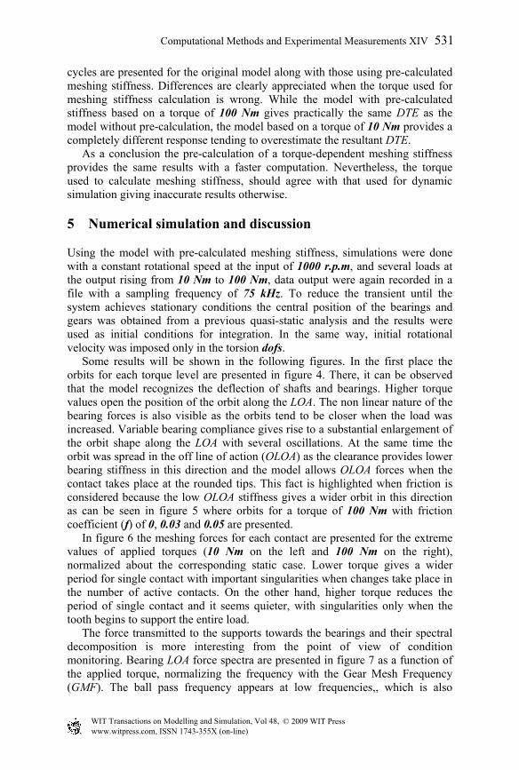
Using the model with pre-calculated meshing stiffness, simulations were done with a constant rotational speed at the input of 1000 r.p.m, and several loads at the output rising from 10 Nm to 100 Nm, data output were again recorded in a file with a sampling frequency of 75 kHz. To reduce the transient until the system achieves stationary conditions the central position of the bearings and gears was obtained from a previous quasi-static analysis and the results were used as initial conditions for integration. In the same way, initial rotational velocity was imposed only in the torsion dofs. Some results will be shown in the following figures. In the first place the orbits for each torque level are presented in figure 4. There, it can be observed that the model recognizes the deflection of shafts and bearings. Higher torque values open the position of the orbit along the LOA. The non linear nature of the bearing forces is also visible as the orbits tend to be closer when the load was increased. Variable bearing compliance gives rise to a substantial enlargement of the orbit shape along the LOA with several oscillations. At the same time the orbit was spread in the off line of action (OLOA) as the clearance provides lower bearing stiffness in this direction and the model allows OLOA forces when the contact takes place at the rounded tips. This fact is highlighted when friction is considered because the low OLOA stiffness gives a wider orbit in this direction as can be seen in figure 5 where orbits for a torque of 100 Nm with friction coefficient (f) of 0, 0.03 and 0.05 are presented. In figure 6 the meshing forces for each contact are presented for the extreme values of applied torques (10 Nm on the left and 100 Nm on the right), normalized about the corresponding static case. Lower torque gives a wider period for single contact with important singularities when changes take place in the number of active contacts. On the other hand, higher torque reduces the period of single contact and it seems quieter, with singularities only when the tooth begins to support the entire load. The force transmitted to the supports towards the bearings and their spectral decomposition is more interesting from the point of view of condition monitoring. Bearing LOA force spectra are presented in figure 7 as a function of the applied torque, normalizing the frequency with the Gear Mesh Frequency (GMF). The ball pass frequency appears at low frequencies,, which is also



-30 -20 -10 0 10 20 30

-20

-15

-10

-5

0

5

10

15

20

Coordenada x [microm]

Coo

rden

ada

y [m

icro

m]

10 [Nm]2030405060708090100

Figure 4: Orbits for several torque levels. Dashed line is the bearing clearance.

28 29 30 31 32 33

8

9

10

11

12

13

14

Coord. x [microm]

Coo

rd. y

[m

icro

m]

28 29 30 31 32 33

8

9

10

11

12

13

14

Coord. x [microm]

Coo

rd. y

[m

icro

m]

28 29 30 31 32 33

8

9

10

11

12

13

14

Coord. x [microm]

Coo

rd. y

[m

icro

m]

Figure 5: Orbit when friction is added; a) f=0; b) f=0.03; c) f=0.05.

0 0.5 1 1.5 2 2.5 3 3.5 4 4.5 50

0.2

0.4

0.6

0.8

1

1.2

1.4

Ciclo de Engrane

Fn/

F0@

10 [N

m]

Contacto 1Contacto 2Contacto 3

0 0.5 1 1.5 2 2.5 3 3.5 4 4.5 50

0.2

0.4

0.6

0.8

1

1.2

1.4

Ciclo de Engrane

Fn/

F0@

100

[Nm

]

Contacto 1Contacto 2Contacto 3

Figure 6: Normalized meshing contact forces; a) 10 Nm; b)100 Nm.

Meshing Cycle Meshing Cycle

Coo

rd.

Coord.



0 2 4 6 8 10 120

20

40

60

80

100

0

10

20

30

40

50

60

70

80

Gear Mesh Frequency

Applied Torque [Nm]

Bea

ring

For

ce [

N]

Figure 7: Spectrum of the bearing forces (b11) in the line of action.

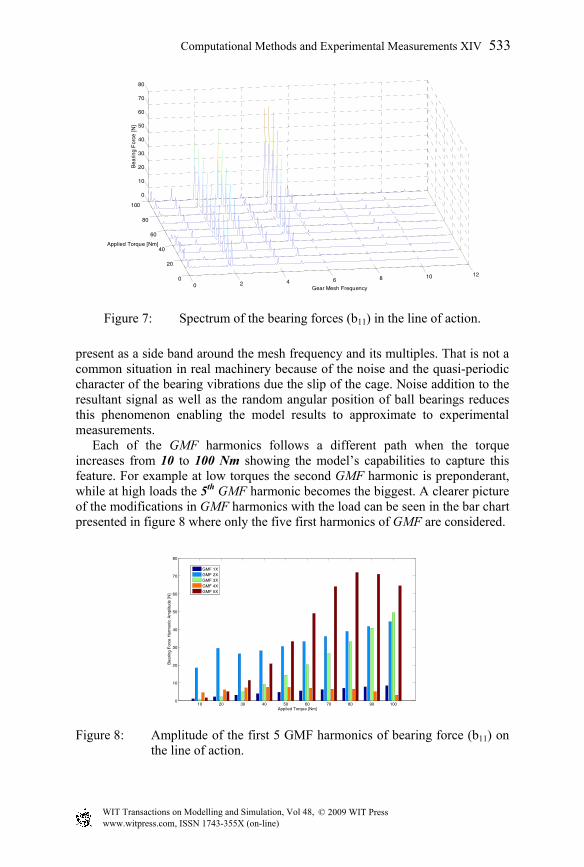
present as a side band around the mesh frequency and its multiples. That is not a common situation in real machinery because of the noise and the quasi-periodic character of the bearing vibrations due the slip of the cage. Noise addition to the resultant signal as well as the random angular position of ball bearings reduces this phenomenon enabling the model results to approximate to experimental measurements. Each of the GMF harmonics follows a different path when the torque increases from 10 to 100 Nm showing the model’s capabilities to capture this feature. For example at low torques the second GMF harmonic is preponderant, while at high loads the 5th GMF harmonic becomes the biggest. A clearer picture of the modifications in GMF harmonics with the load can be seen in the bar chart presented in figure 8 where only the five first harmonics of GMF are considered.

10 20 30 40 50 60 70 80 90 1000

10

20

30

40

50

60

70

80

Applied Torque [Nm]

Bea

ring

For

ce H

arm

onic

Am

plitu

de [N

]

GMF 1XGMF 2XGMF 3XGMF 4XGMF 5X

Figure 8: Amplitude of the first 5 GMF harmonics of bearing force (b11) on the line of action.



6 Conclusions

A model for the dynamic analysis of a gear transmission supported by bearings was presented. This model was based on an efficient formulation and solution of the meshing contact forces with a non-linear model for bearings. In order to improve the computation time, a pre-calculated value for meshing stiffness was obtained, simplifying the resultant equations system. Careful selection of the torque should be done in order to obtain accurate results. Special attention should be paid when the load cannot be considered stationary, using in these cases the original model. The model features were demonstrated with a simple transmission paying particular attention to the bearing force spectrum variation with the load and showing the capability of the model to capture this behaviour.

Acknowledgements

This paper has been developed in the framework of the Project DPI2006-14348 funded by the Spanish Ministry of Science and Technology.

References

[1] Ozguven, N. H., Houser, D. R., Mathematical Models used in gear dynamics – a review, Journal of Sound and Vibration, 121(3), pp. 383-411, 1988.

[2] A. Kahraman, R. Singh, Interactions between time-varying mesh stiffness and clearance nonlinearities in a geared system, Journal of Sound and Vibration, 146(1), pp 135-156, 1991.

[3] S. Fukata, E. H. Gad, T. Kondou, T. Ayabe, H. Tamura, On the radial vibrations of ball bearings (computer simulation), Bulletin of the JSME, 28, pp. 899 - 904, 1985.

[4] F. Viadero, A. Fernández del Rincón, R. Sancibrian, P. García Fernández, A. de Juan, A model of spur gears supported by ball bearings, WIT Transactions on Modelling and Simulation, 46, pp. 711- 722, 2007.

[5] A. Fernández del Rincón, F. Viadero, R. Sancibrian, P. García Fernández, A. de Juan, Esfuerzos de contacto en engranajes exteriores de dientes rectos con defectos, soportados mediante rodamientos, 8º Congreso Iberoamericano de Ingeniería Mecánica, CIBIM8, Cuzco (Perú), 2007.

[6] A. Andersson, L. Vedmar, A method to determine dynamic loads on spur gear teeth and on bearings, Journal of Sound and Vibration, 267(5), pp. 1065-1084, 2003.

[7] Tedric A. Harris, Rolling Bearings Analysis, John Wiley & Sons Inc., 2001. [8] F. Chaari, W. Baccar, M. S. Abbes, M. Haddar, Effect of spalling or tooth

breakage on gearmesh stiffness and dynamic response of a one-stage spur gear transmission, European Journal of Mechanics A/Solids, (2008).

[9] S. Wu, M. J. Zuo, A. Parey, Simulation of spur gear dynamics and estimation of fault growth, Journal of Sound and Vibration, (2008).



a dynamic model for the study of gear transmissions · a dynamic model for the study of gear ......

Documents