a dynamic, interactive approach to learning engineering and … · a dynamic, interactive approach...
TRANSCRIPT

A Dynamic, Interactive Approach to Learning
Engineering and Mathematics
Jason Ross Beaulieu
Thesis submitted to the Faculty of
Virginia Polytechnic Institute and State University
in partial fulfillment of the requirements for the degree of
Master of Science
In
Mechanical Engineering
Brian Vick, Chair
Srinath Ekkad
Robert L. West
April 19, 2012
Blacksburg, VA
Keywords: Mathematica, CDF, Computable Document Format, Interactive Learning,
Dynamic Learning
© Copyright 2012, Jason Beaulieu

A Dynamic, Interactive Approach to Learning
Engineering and Mathematics
Jason Ross Beaulieu
Abstract
The major objectives of this thesis involve the development of both dynamic and
interactive applications aimed at complementing traditional engineering and science
coursework, laboratory exercises, research, and providing users with easy access by
publishing the applications on Wolframs Demonstration website. A number of
applications have been carefully designed to meet cognitive demands as well as provide
easy-to-use interactivity.
Recent technology introduced by Wolfram Mathematica called CDF (Computable
Document Format) provides a resource that gives ideas a communication pipeline in
which technical content can be presented in an interactive format. This new and exciting
technology has the potential to help students enhance depth and quality of understanding
as well as provide teachers and researchers with methods to convey concepts at all levels.
Our approach in helping students and researchers with teaching and understanding
traditionally difficult concepts in science and engineering relies on the ability to use
dynamic, interactive learning modules anywhere at any time.
The strategy for developing these applications resulted in some excellent
outcomes. A variety of different subjects were explored, which included; numerical
integration, Green's functions and Duhamel's methods, chaotic maps, one-dimensional
diffusion using numerical methods, and two-dimensional wave mechanics using
analytical methods. The wide range of topics and fields of study give CDF technology a
powerful edge in connecting with all types of learners through interactive learning.

iii
Acknowledgements
I would like to begin by thanking the members of my committee, Dr. Srinath
Ekkad and Dr. Bob West. I appreciate your time from your busy schedules to review my
work. Also, I would like to express my deepest gratitude to Dr. Brian Vick. You have not
only been an amazing mentor, but most importantly a friend and someone who I will
always look up to.
A special thanks to the CIDER (Center for Instruction Development and
Education Research) for the Instructional Enhancement, Innovation and Exploration grant
that helped me complete my work.
And a final thank you to my family and friends. It would have been hard to do the
things I've done without the love and support of you all.

iv
Preface
This thesis was intended to be viewed using the CDF version located on the
Virginia Tech ETD website. It allows for the individual interactivity of each learning
module. Please download either Mathematica 8+ or Mathematica’s free CDF Player to
view the document.

v
Table of Contents
Chapter 1: Introduction…………………………….……………………….………….1
1.1 Project Description………………….………..………………………………..1
1.2 Motivation………………………..……………….…………...….…...………2
1.3 Objectives………………………….…………………………….……………3
1.4 Outline…………………………………………...……….……..……..………4
Chapter 2: Literature Review……………………..………………………….…...…….5
2.1 Interactive versus non-interactive displays……….…….…………….……….5
2.2 Design considerations…………………………….……….……….………….7
2.3 Effectiveness ……………………………………….……..…….………...…..9
2.4 Implementation……………………….…………………….……..…………11
Chapter 3: Dynamic, Interactive Learning through Mathematica………..…...…...13
3.1 Numerical Integration……………………………………………….……….13
3.2 Discrete Green's Function and Duhamel's Methods…….…….….……….....16
3.3 Dynamics of Chaotic Maps…………………………….………..………..….21
3.4 One-Dimensional Diffusion………………………...……………...……...…24
3.5 Wave Mechanics…………………………………………………..……...….29
Chapter 4: Conclusions..………………...………………...………….…………….…33
Publications………………………………………………...……………………….…..35
References……………………………………………………...………………………..36

vi
Appendix A:
Equations & Derivations……………………………….……………………………....39
A1: Numerical Integration……………....……………….………………………39
A2: Discrete Green's Function and Duhamel's Methods…….…………………..40
A3: Dynamics of Chaotic Maps…………………….……………………………42
A4: One-Dimensional Diffusion…………………….…………………………...43
A5: Wave Mechanics………………….……………………………...………….45
Appendix B:
Mathematica Source Code……………………….……..…………...………………....49
B1: Numerical Integration………………..………………………………...……49
B2: Discrete Green's Function and Duhamel's Methods……….…….…...……..51
B3: Dynamics of Chaotic Maps…………………..……………………...………54
B4: One-Dimensional Diffusion………………..………………………...……...57
B5: Wave Mechanics……………..……...………………………………...…….62
vii
List of Figures
Figure 1: Numerical integration presentation……………………..….…………………14
Figure 2: Integration rule example..………………………………………..……………14
Figure 3: Numerical integration segments example………………………..….…….….15
Figure 4: Discrete Green's function and Duhamel's methods presentation…….…….….17
Figure 5: Discrete Green’s function and Duhamel’s method ODE example……..….….18
Figure 6: Discrete Green’s function and Duhamel’s methods example……………..….19
Figure 7: Discrete Green’s function and Duhamel’s methods segments visualization….20
Figure 8: Dynamics of chaotic maps presentation………………………………..…..…21
Figure 9: Chaotic maps driving parameter example….…………………………..…..…22
Figure 10: Initial condition sensitivity for chaotic maps……..…………………….…...23
Figure 11: One-dimensional diffusion presentation…………….………..………..……26
Figure 12: Boundary conditions for one-dimensional diffusion.…….…………….…...28
Figure 13: Wave mechanics presentation..………….………………….....…………….31
Figure 14: Boundary conditions for wave mechanics……………………………..……32
Figure 15: Aspect ratio for wave mechanics…………….….…………………………..32
viii
Nomenclature
Density,
Heat Capacity,
Temperature,
Thermal Conductivity,
Heat Transfer Coefficient,
Heat Flux,
Surrounding Bulk Temperature,
Non-Dimensional Damping
Non-Dimensional Wave Speed
A Aspect Ratio

1
1
Introduction
1.1 Project Description
Visual learning has increased dramatically with the growth of high powered, low
cost computing. Resources ranging from online videos to individual dynamic learning
modules provide an alternative approach to learning various technical concepts.
However, claims about technological advances that can solve many educational problems
have been made throughout the century. Thomas Edison was quoted in saying "I believe
that the motion picture is destined to revolutionize our education system and that in a few
years it will supplant largely, if not entirely, the use of textbooks" [Hegarty, 2004]. As we
now know, this was not the case as textbooks are still used in most educational systems.
On the other hand, this does lead us into an important consideration for understanding
what conditions must be met to fully utilize recent technological advances, most notably
Mathematica' s Computable Document Format, and their effectiveness in learning and
how they may benefit traditional teaching practices.
This project focuses around the use of a recent technology called CDF
(Computable Document Format) that was released by Wolfram in the spring of 2011.
CDF Player is a free application that allows anyone to interact and explore with
Mathematica notebooks. The dynamic, interactive visualization is utilized in the CDF
format and has the potential to give a deeper understanding of historically difficult
concepts. This project is intended to add content to the science of visual learning through
dynamic, interactive applications.
Before we begin, it is important to define what a dynamic, interactive presentation
is. The term dynamic refers to the ability of an application to update information as soon
as changes occur in the input. Interactivity allows the user to define what changes are
being made and at what speed. Therefore, a dynamic interactive presentation can be

2
defined as an application that continuously updates the output as a user changes the input.
The work done in this thesis uses Mathematica's powerful computing software to create
individual learning modules.
1.2 Motivation
In order to be a successful well-rounded engineer, it is important to develop a
thorough understanding of both abstract and applied concepts. The current curriculum at
most engineering universities presents students with demanding coursework at a
relatively fast pace. The level of difficulty and amount of coursework a student is asked
to learn is within itself a difficult feat to overcome. It is unreasonable for a student to
become proficient in every subject he or she learns throughout their academic career.
However, it is important for a student to leave with a broad understanding of each
subject. On the other hand, it is often difficult for a professor to communicate technical
content on an intuitive level through conventional lectures. Therefore, it is important to
provide a resource that can complement traditional teaching methods in order to help
educators and provide students with a solid education.
For some educators, providing engineering students with a strong theoretical base
and good engineering skills come from four essential components [Wittenmark &
Haglund et al., 1998]:
• Theory
• Good engineering tools
• Engineering judgment
• Understanding
First, theory is provided by the professor via lectures and an adequate textbook.
Additionally, assigning coursework requires the student to practice and use good problem
solving techniques. However, the ability to solve a differential equation or other complex

3
problems does not necessarily entail a detailed understanding of the science or
mathematics.
Secondly, good engineering tools can enhance the progress of learning. Computer
software such as Mathematica, MATLAB, and AutoCAD provide students with the
necessary tools used to solve complex problems and gain experience with industrial
software. Additionally, state of the art lab equipment will give accurate results which
connect the analytical/theoretical analysis to experimental results.
Engineering judgment is an essential aspect to a successful engineer. Companies
can save time and money if proper theory and judgment are used. In practice, engineering
judgment can be a relatively hard topic to teach. It can be considered as an intuitive
attribute of an engineer. Nonetheless, one can gain experience in engineering judgment
by laboratory exercises, technical projects, and industrial experiences.
Finally, the last ingredient necessary for a strong theoretical base and good
engineering skills is a strong understanding of the material. The traditional approach
relies on the student to take the resources provided by a textbook and a professor via
lectures and gain a thorough understanding of the material. However, it should be
possible for a student to be able raise questions on what-if scenarios. Our approach in
helping students and researchers with understanding difficult concepts in science and
engineering relies on the ability to use dynamic, interactive learning modules anywhere at
any time. Users are able to control several variables and see how equations and processes
change. It should be noted that this is not intended to compete with tradition learning
systems, but instead is intended to complement them.
1.3 Objectives
The main objectives of this project involve developing applications that are both
dynamic and interactive using Mathematica's CDF technology. These applications are

4
intended to provide complementary material for traditional lectures, coursework,
research, and laboratory exercises. The goals we worked to achieve are:
Create applications to use in a research environment
Develop applications for use in traditional engineering and science courses
Develop virtual labs to compliment traditional laboratory courses
Publish applications on open websites, particularly on the Wolfram
Demonstration Site
1.4 Thesis Outline
Chapter 2 is a literature review on several aspects related to dynamic, interactive
learning modules. We present design considerations, effectiveness, and supporting
research for interactive applications.
Chapter 3 presents the reader with various interactive, dynamic applications
specifically designed to enhance the learning and understanding of advanced concepts.
The subjects range from a wide variety of mathematical and engineering concepts which
include:
• Numerical Integration
• Green's Functions and Duhamel’s Method
• Chaos
• Iterated Maps
• Finite Difference
• Numerical Methods
• Heat Transfer
• Orthogonal Function Expansion
• Analytical Methods
• Wave Mechanics
Lastly, chapter 4 provides a summary of the thesis and directions for future work.
Source code materials and derivations used in this thesis are included within the
appendices.

5
2
Literature Review
The next generation of scientists and engineers are faced with increasingly
challenging problems. It is important for educators and researchers to use the resources
available to them in order to provide a solid understanding of fundamental concepts to
their students and/or collaborators. In this review, we will mainly focus on dynamic,
interactive learning modules that can supplement lectures, textbooks, research, and
laboratory experiments. Considerations on the on the design approaches, effectiveness,
and implementation will be explored. Also, we will discover the advantages and
disadvantages of using dynamic, interactive displays. Finally, we will discuss future
implications and then begin presenting the main work of the thesis.
2.1 Interactive versus non-interactive displays
Numerous studies have reported that students learn better from text and pictures
than from text alone [Rasch & Shnotz, 2009]. However, it is unclear if that theory can be
extended to ‘students learn better from interactive displays than from non-interactive
displays.’ So far, the findings have mixed results. Research on this matter is still in the
beginning stages for understanding what conditions must be met in order for this
technology to enhance comprehension and learning. To begin, an overview of some
advantages and disadvantages of several types of displays are discussed.
Non-interactive displays
Non-interactive dynamic displays can include a variety of media including
animations and movies. These types of displays play at a constant rate defined by the
author. Once the video advances beyond a frame, that information is no longer available.
This results in heavy demands on memory. It is well known in literature that memory has
6
a limited capacity when dealing with new information. In fact, without rehearsal,
information in working memory is lost within 20 seconds [Peterson & Peterson, 1959].
Therefore, animations and movies that convey technical concepts may not be beneficial
to the learner. On the other hand, static displays allow the viewer to re-inspect various
parts of the display as frequently as needed to gain a comfortable understanding.
Research has concluded that displaying the corresponding states of a concept
simultaneously with static pictures would provide a much better understanding for
technical concepts [Schnotz & Lowe, 2008].
Interactive displays
On the other hand, interactive dynamic displays allow the user to define the speed
based on their own comprehension. They enable the user to adapt to their own personal
constraints on perceptual and cognitive processing by slowing down or speeding up the
rate of the display. Also, they allow the user to test various hypotheses about the
processes by defining parameters of the display accordingly. This puts fewer demands on
memory and more focus on understanding. Furthermore, research has concluded that
when interacting with dynamic displays, viewers are much more active in the learning
process [Hegarty, 2004].
Becoming comfortable with new software will take time and can vary from
student to student. The "ramp up time", or time to become comfortable with software, can
be considered disadvantageous. Most students are familiar with PowerPoint or movie
presentations and therefore do not need time to begin learning. Therefore, it is important
to consider ramp up time when designing the GUI (graphical user interface).
Furthermore, manipulation of a dynamic, interactive application requires additional
cognitive resources to determine what parameters to move and locating the associated
controls. In other words, interactivity of a dynamic display may ruin its advantages by
imposing additional loads on working memory capacity.

7
2.2 Design considerations
Several variables must be taken into account when designing an effective
dynamic, interactive learning module. Each application needs to be carefully designed to
match the needs of the users. In this section, we will discuss several considerations that
are necessary for creating useful applications. Also, we will look into research conducted
by M. Hegaty and Narayanan on design approaches for interactive presentations.
One important design feature is that the application should be able to be used
intuitively, or with limited guidance. This takes careful planning and skill throughout the
design process. There are several reasons for this. First, almost nobody reads a user
manual. Second, each module will be used without supervision. Third, users can be very
impatient.
Each of the modules designed in this project were carefully designed with
considerations towards the user and the environment it will be used. However, the layout
and graphics all follow the same relative format. These guidelines provide a useful
technique in design considerations:
• Audience - previous knowledge of ideas about specific concept
• Content - only one idea per module
• Color coding - understanding connections between concepts
• Layout - familiarity with graphic interface and interactivity
• Controls - easy to use controls like drag or click with a mouse
Research on design considerations was conducted by Narayanan and Hegarty
from the Intelligent & Interactive Systems Laboratory at Auburn University [Narayanan
& Hegarty, 2002]. In their research, they examine the assumption that interactive
graphical presentations that are designed using a cognitive approach are more effective
than commercially available material. A series of experiments compared the two
applications.

8
Design
The study began with ninety-four undergraduate students participating voluntarily
for a credit in a psychology course. The group was then split into four separate groups of
24, 24, 23, and 23 students. The first group was asked to study material on the
mechanical operation of a flushing cistern. This material was an interactive presentation
designed using the cognitive design guidelines. The second group was asked to study the
exact same material in printed form. The third and fourth groups studied another source
on the mechanical operation of a flushing cistern from "The New Way Thinks Work"
software by Macaulay. Each group was asked to study either the interactive software or
the static version. The main differences in the two visual presentations are how they were
designed. The Hegarty and Narayanan presentation was designed using guidelines from a
cognitive model. On the other hand, the material by Macaulay was designed to be
entertaining.
The students were asked to study the material until they felt comfortable with the
behavior of the system. They were then asked a series of questions related to the
operation and troubleshooting of the system. The study found some interesting results.
Results
The experiment yielded significant differences on the comprehension of the
dynamics of the mechanical system. Students who learned from the cognitive designed
media included more description on the step by step process of the flushing cistern.
Moreover, students who learned from the cognitive design were better at stating various
functions of the components of the system. However, it is important to note that students
who learned from both the interactive and static versions of the cognitive design had
similar performance on learning.
9
Overall, the results let us come to the conclusion that cognitive process models for
interactive presentations are superior to the commercially available materials. However,
we can also assume that the type of media, i.e. interactive and static presentations, does
not prove to have any advantages over one another. Instead, the more important factor in
cognitive design guidelines is the content of the material. This result was also confirmed
by [Rasch & Schnotz, 2009]. Another interesting result is that interactive demonstrations
tend to take more time to comprehend. This may be due to the time needed to learn the
software or the interaction with the controls.
2.3 Effectiveness
As the use of technology in academic environments increases, so will the use of
interactive displays. However, the effectiveness of visual learning environments must be
accounted for when deciding to implement interactive displays. Unfortunately, there have
been many difficulties for researchers to measure effectiveness. Reasons include the vast
number of topics an interactive display may include. Some topics may be better presented
more effectively through different media outlets. Furthermore, there is no standard on
design guidelines for each application. Researchers use their own design approaches
which vary from other designs and therefore the results are slightly different. Also,
interactive applications require the user to adapt to a discovery learning process. This
type of learning is demanding and can be problematic.
The process of discovery learning involves the steps of scientific reasoning:
stating a hypothesis, designing an experiment, evaluating the results, and reformulating
the hypothesis. This type of learning through simulation-based discovery has a highly
constructive potential [Rieber et al., 2004]. Interactive modules require a move from a
teacher-student dependence to a teacher-student independence, which can lead to deeper
understanding of the concept [Schnotz et al., 2009]. However, the learner encounters
many problems throughout the process of discovery learning. For instance, learners have
difficulties in defining appropriate hypothesis and evaluating results of the interactive
10
application [Bodemer et al., 2005]. Furthermore, the user has difficulties in planning their
interactions with interactive displays in a systematic, goal-orientated way. Therefore,
users tend to randomly interact with these types of applications [de Jong & Jooligen,
1998]. However, some researchers have attempted to measure the effectiveness of
complimenting this type of media in traditional learning environments.
Bodemer and his colleagues conducted research on the effectiveness of visual
learning though dynamic, interactive applications [Bodemer et al, 2004]. In two
experiments, the research group set out to determine if the implementation of interactive
applications increased learning. The theory, design, and results will be presented next.
Theory
Cognitive load theory provides various guidelines to assist in the design and
presentation of information to increase learning performance. Based on the assumptions
of (1) limited working memory and (2) unlimited long-term memory, the cognitive load
theory provides instructions that do not overburden a learners working memory
[Baddeley, 1986]. By implementing this theory, the design of each experiment revolved
around the use of several types of media in the learning system, i.e. text, static pictures,
dynamic and interactive visualizations.
Design
Two experiments were conducted with 165 students from the University of
Freiburg in Germany. The study focused on learning the principles behind a tire pump. In
the first experiment, 81 students were presented with static representations of a tire pump.
In the second experiment, students 84 students were presented with static representations
as well as dynamic, interactive visualizations. Half of the students in experiment two
were taught how to interact with the visualizations in a systematic and structured way, the
other half were not. Every student had a background in social sciences and knew what a

11
tire pump was. They were asked a series of questions before and after the study. The
students were paid for their participation.
Results
In the pre-test, it was found that there were no statistically significant differences
between each group. On the other hand, the post-test yielded some interesting results.
The experiments revealed that dynamic, interactive media can improve learning
by encouraging and teaching students how to interact and properly use these
presentations. However, presentations that are in combination with other kinds of media
can be very demanding and overburden cognitive abilities of a learner. Because of this,
leaners tend to limit their attention to the visualizations and do not interact with them in a
structured way. As a consequence, learners do not relate different sources of information
to create an overall mental representation.
Overall, this research added some important information in the study of
interactive presentations. From the results, we can conclude that proper instruction and
guidance for using dynamic, interactive displays can benefit the learning process. Also,
these displays should be used in coordination with traditional learning environments. In
the end, these results confirm that using dynamic, interactive learning modules increase
learning and understand.
2.4 Implementation
The most useful and greatest attribute about dynamic, interactive displays is
requiring only two components, the user and a computer. Essentially, this allows the user
to learn anywhere at any time. To implement our ideas, we use the new technology
offered by Wolfram Mathematica called CDF (Computable Document Format). These

12
programs are available to anyone that has Mathematica 8 or Mathematica’s free CDF
Player.
Access, availability, and simplicity are crucial when deciding to implement visual
learning as a way to compliment research or lectures. Access to CDF documents depends
on the author or other factors such as research or institutional limitations. However,
Wolframs Demonstration Site provides an easy and free way to publish and access a vast
expanse of interesting applications. Availability comes from the computer and internet
access. It is important to provide an easy and constant availability to these applications.
Lastly, simplicity comes from the selection of software. Complicated downloads and
difficult user interfaces can be a turn off for a user. In this case, CDF player is an easy,
one-step download that opens the door for constant supply of content.
Furthermore, it was found in literature that it is important to instruct and
encourage learning through interactive presentations as well as provide other traditional
learning materials. Mayer and Chandlder found that learning increases when the learner
is given the opportunity to process static information before viewing the dynamic,
interactive presentations [Mayer & Chandler, 2001]. Also, it has been suggested that a
structured learning environment would best support interactive applications [Bodemer, et
al, 2004]. Therefore, using these applications would work best as supplemental materials
in traditional lectures. These lectures provide students with instructional guides
(professor) and static visual representations (textbooks).

13
3
Dynamic, Interactive Learning through Mathematica
In this section, we present different dynamic, interactive modules created to
complement conventional lectures, laboratory exercises, and research. Each module will
have a brief explanation of the concept and its intended use. To ensure the consistency
with the CDF version of this document, please click on the
Evaluation Evaluate Initialization Cells
in Mathematica's menu bar.
3.1 Numerical Integration
Numerical integration is a method used to calculate an approximate value of the
definite integral:
∫
.
It is a fundamental concept for any engineering student to understand. The
motivation of this application is to provide students in an introductory math and science
course with an easy-to-use interactive application. This demonstration compares various
Newton-Coates methods to approximate the integrals of several different functions over
the interval [a , b]. The details of each method can be found in Appendix A1.
Figure 1 presents the dynamic, interactive learning module designed for
numerical integration. Some interesting and important features to interact with are the
integration rules, segments, and the different functions.

14
Figure 1: Numerical integration presentation
Integration rule: The integration rule allows the user to see how each respective rule
fits with a certain function. It may not be clear to a beginning student that the
Simpson's
rule (2
nd order) with one segment will give an exact approximation to a
2nd
order polynomial function. Also, one can visualize how the error typically
decreases as the order of the method is increased, as demonstrated in figure 2.
Trapezoid:
1st Order
Simpson’s 1/3:
2nd
Order
Simpson’s 3/8:
3rd
Order
Boole’s:
4th
Order
Figure 2: Integration rule example. Each image has four segments for each method. Notice how the error
decreases as the order of the method increases.

15
Segments: The design of this demonstration allows easy visualization of each
segment, i.e. alternating light blue and dark blue, and how each segment fits a
particular part of the function. Users can visualize how the trapezoid rule can be a
very crude approximation with a low number of segments but becomes increasingly
accurate as the number of segments increase. Usually, more segments leads to a more
accurate approximation of the integral. For a large number of segments, numerical
integration is almost perfect.
1 segment 2 segments 4 segments 8 segments
Figure 3: Numerical integration segments example
Function: Different functions were picked to offer a variety of behaviors. The 2nd
order polynomial is a relatively easy integral to calculate and higher order methods
give an exact approximation. The exponential function tends to require more
segments and higher order methods. The oscillator can give terrible approximations if
the choice of method and segments are not chosen properly.
Polynomial:
Oscillator:
Exponential:
Using this demonstration allows the user to visualize certain details and truly
understand numerical integration. Overall, this application provides an insight to
numerical integration that is difficult to be achieved using static documents only.
0 1x
1.0
0.5
0.5
1.0
f x
I 0.212error 100.

16
3.2 Discrete Green’s Function and Duhamel’s Methods
It is often difficult for students to get an understanding of Green's functions and
the Duhamel’s method for solving differential equations. As a result, the idea came about
to create a visual aid to complement lectures for advance mathematics or engineering
science courses.
This demonstration shows how to find approximate solutions to linear ordinary
differential equations using two methods:
1. The discrete Green’s function method, in which the source is approximated as a
sequence of pulses;
2. The discrete Duhamel’s method, in which the source is approximated by a
sequence of strips.
The complete solution is approximated by a superposition of solutions for each
individual pulse or strip. As the limit of the number of segments tends to infinity, the
pulse and strip methods approach the continuous Green’s method and Duhamel’s method,
respectively.
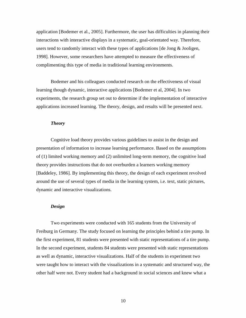
Figure 4 represents the dynamic, interactive learning module for discrete Green's
functions and Duhamel’s methods. In the graphs:
Solid, filled, red lines represent the exact source and response;
Thin, black, dashed lines represent the individual sources and responses to
each pulse or strip;
Thick, black, dashed lines represent the total approximate source and
response.
17
Figure 4: Discrete Green's function and Duhamel’s methods presentation
The idea behind this application is to show that linear problems can be
constructed by using a linear combination from simpler subproblems. If the forcing
function is expressed as:
∑
Then the total solution can be expressed as:
∑
Where is the response to . In this demonstration, we have decomposed the forcing
function, , as a sequence of either pulses or strips. This method can be extended to
solve problems that contain other types of forcing functions such as volumetric sources,
18
surface sources, and initial conditions. The approximate solution with multiple forcing
functions can be found by superimposing each response to the individual forcing
functions.
The important controls to explore are the ODE, the method, and the segments, and
the source.
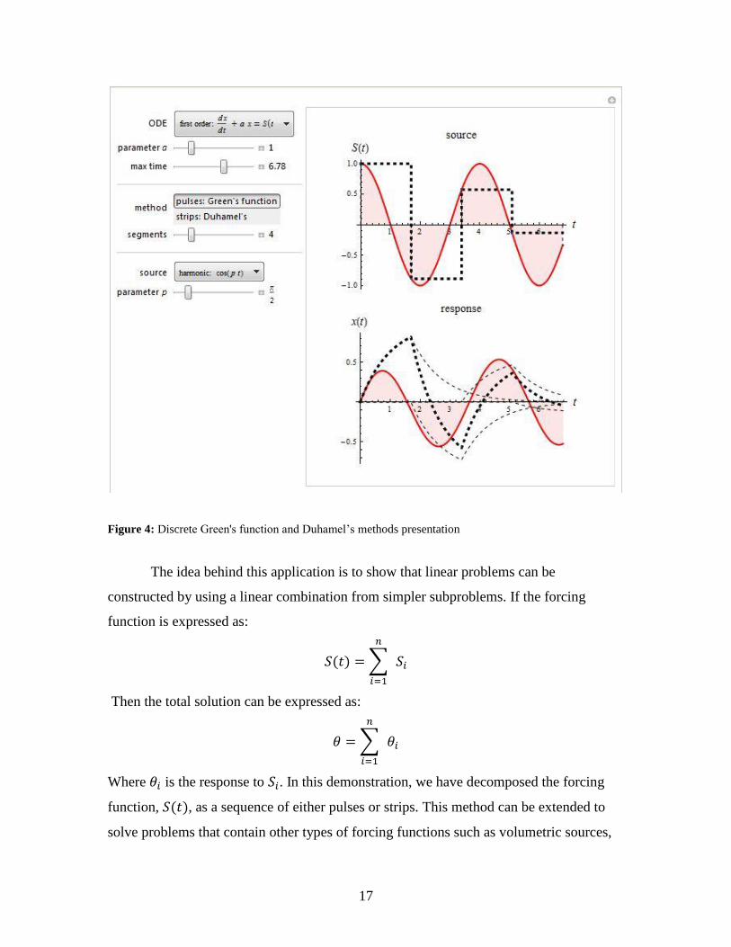
ODE: The differential equations that can be explored are a linear first order
differential equation and a linear second order differential equation. These types of
equations are found throughout most all applied and theoretical mathematics courses.
Each equation provides a different insight into the overall behavior of the methods.
1st Order ODE
2nd
Order ODE
Figure 5: Discrete Green’s function and Duhamel’s methods ODE example. The parameter, a, is equal to
0.7 and the number of segments is equal to 6.
19
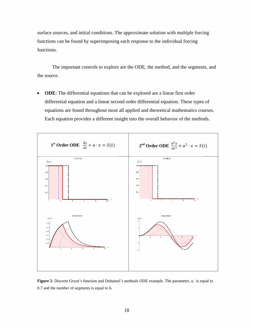
Method: The pulse method uses the linearity property to construct the total response
by the addition or superposition of the responses to all the pulses. This method is a
discrete version of the Green's function technique. In the limit as , the method
reduces to the usual Green's function method. Similarly, the strip method finds the
total response by the superposition of responses to all the strips. This method is
particularly useful in the time variable rather than the spatial variable, because time
runs indefinitely, while space is typically limited to a finite region. This method is a
discrete analog of Duhamel’s method. By taking the limit as , Duhamel's
method is obtained. Each method has its advantages and disadvantages, but they
result in the same level of approximation.
Discrete Duhamel’s: Strips Discrete Green’s functions: Pulses
Figure 6: Discrete Green’s function and Duhamel’s methods example.

20
Segments: It is interesting to see how the number of segments affects the
approximation. It is not always the case that more segments leads to a more accurate
approximation. Instead, it is more important to fit the segments in a logical way in
order to get a fairly accurate representation of the forcing function. Figure 4
demonstrates this concept.
3 Segments 8 Segments
Figure 7: Discrete Green’s function and Duhamel’s methods segment visualization. Notice how there is a
better approximate response with three segments than with eight segments. More segments do not always
lead to a better approximation of the source and response. Therefore, it is more important to consider how
the pulses fit the source.
21
3.3 Dynamics of Chaotic Maps
Iterated maps can exhibit a spectrum of dynamic and unusual behavior. This
demonstration shows the relationships of the various iterated maps and their associated
orbit, final state diagram, cobweb plot, and Lyapunov exponent. This demonstration was
designed for any course teaching mathematical modeling techniques or the behavior of
non-linear dynamics and chaos. The details of each concept, i.e. orbit, final state plot,
Lyapunov Exponent, and cobweb plot, can be found in Appendix A3. The specific
iterated functions studied in this application are:
Logistic map:
Quadratic map:
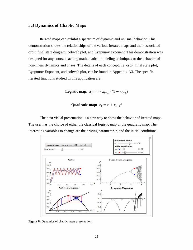
The next visual presentation is a new way to show the behavior of iterated maps.
The user has the choice of either the classical logistic map or the quadratic map. The
interesting variables to change are the driving parameter, r, and the initial conditions.
Figure 8: Dynamics of chaotic maps presentation.

22
The interactivity and layout of this application allows the user to visualize the
connections between the different dynamics of the system. Some interesting features of
each map can be found by manipulating the controls.
Driving parameter: By varying the parameter, , you can explore the bifurcations
and the onset of chaos for each iterated map. It is interesting to start out with a low
value of and watch a period-doubling sequence occur. For the logistic map, at
a stable final state bifurcates into two final states. As is driven to higher values, a
sequence of period doubling bifurcations occur until chaotic behavior is reached at
.
Figure 9: Chaotic maps driving parameter example.
23
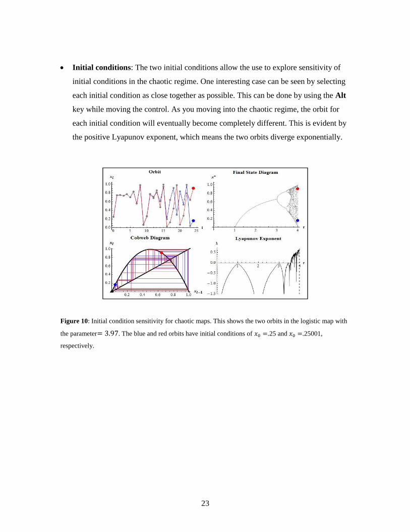
Initial conditions: The two initial conditions allow the use to explore sensitivity of
initial conditions in the chaotic regime. One interesting case can be seen by selecting
each initial condition as close together as possible. This can be done by using the Alt
key while moving the control. As you moving into the chaotic regime, the orbit for
each initial condition will eventually become completely different. This is evident by
the positive Lyapunov exponent, which means the two orbits diverge exponentially.
Figure 10: Initial condition sensitivity for chaotic maps. This shows the two orbits in the logistic map with
the parameter . The blue and red orbits have initial conditions of .25 and .25001,
respectively.
24
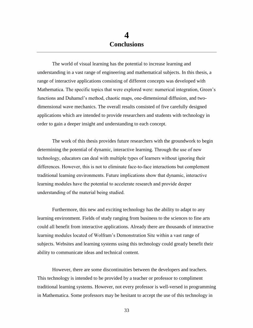
3.4 One-Dimensional Diffusion
Numerical methods are used when analytical solutions become difficult or
impossible to find because of complicated geometry, nonlinear properties, or nonlinear
boundary conditions. The most popular numerical methods are finite differences, finite
elements, and boundary elements. In this demonstration, we introduce an application that
was designed to solve the one-dimensional diffusion equation using an implicit finite
difference algorithm. The discretized equations and source code can be found in appendix
A4 and B4, respectively. The graphical user interface was designed to give an easy-to-use
interactivity to visualize the response from changing the various parameters and forcing
functions.
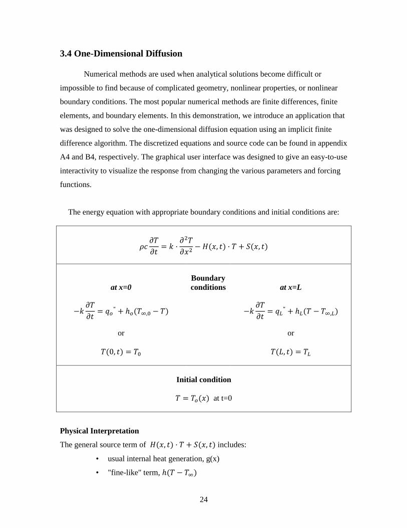
The energy equation with appropriate boundary conditions and initial conditions are:
at x=0
or
Boundary
conditions
at x=L
or
Initial condition
at t=0
Physical Interpretation
The general source term of includes:
• usual internal heat generation, g(x)
• "fine-like" term,

25
• any other linear physics; e.g., chemical reactions
The term:
represents the rate of change in energy with respect to time.
The term:
represents the net conduction effect. Mathematically it describes the concavity of the
temperature profile at one point to the temperature at neighboring points.
The next demonstration is a bit more detailed than the previous demonstrations.
However, it is a useful tool for visualizing and solving different case studies for the one-
dimensional diffusion equation. This application is intended for researchers or advanced
students who have a good understanding of heat transfer. The robust nature of this finite
difference code allows for studies of numerous heat transfer cases.

26
Figure 11: One-dimensional diffusion presentation.
In order to understand the layout, we have arranged the graphical user interface
into logical sections. Each part contributes to the understanding of heat transfer in a
different way.
Numerical parameters: The numerical parameters include (1) the time step, , (2)
the grid size, ii, and (3) max time step, pmax. They are the parameters that contribute
to the accuracy of when solving the diffusion equation in the finite difference
algorithm.
27
Material properties and Geometry: Material properties include (1) the heat
capacity, c, (2) the density, , and (3) the thermal diffusivity, k, and (4) the length, .
These properties allow for studies of numerous types of materials, i.e. gases; liquids;
and solids. They contribute to the understanding of how different materials behave.
Note that only the product is needed.
Initial conditions: The initial temperature distribution of the system is an important
feature of this demonstration. The user has the option of a spatially localized or
constant temperature distribution subject to any magnitude. The constant temperature
distribution can be obtained by setting to 0% and
to 100%.
Volumetric source, : The volumetric source includes heat generation and is
dependent on the convective environment along the one-dimensional slab. It is
defined as:
Where is internal heat generation, P is the perimeter of the slab, is the cross-
sectional area, and is the temperature of the external environment.
Proportional losses, : The proportional losses can be considered a parameter of
the external environment. It is defined as:
Boundary conditions: The middle section presents the user with the option to choose
what type of boundary conditions as well as the magnitude of several variables
associated with the specific boundary condition. Figure 12 shows the how this
demonstration can help in understanding the behavior of different boundary
conditions.

28
|
|
|
|
|
|
Figure 12: Boundary conditions for one-dimensional diffusion. The initial condition is a unit step pulse in
located in the center. The volumetric sources and proportional losses are both zero.
Solution plot: The final solution corresponding to the inputs from the first graphical
user interface is presented in the last section. The layout of this demonstration allows
for the immediate calculations as the parameters/variables are changed. However, the
solution will not re-calculate as the time-steps are varied.
Overall, this demonstration allows for a quick and relatively easy method of
exploring the many aspects related to the one-dimensional diffusion equation. It is
suggested to provide guidelines and instructions on how to properly learn from this
application. The depth of understanding and insight this application provides can be a
useful tool in many heat transfer courses.

29
3.5 Wave Mechanics
This demonstration shows the solution of the two-dimensional wave equation
subjected to an instantaneous hammer hit centered at the source point location with zero
initial displacement and velocity. The user has a choice of free or fixed boundary
conditions. A fast and accurate solution was obtained by using the orthogonal function
expansion method. The detailed derivation can be found in appendix A5. This application
originated around the idea of a virtual lab intended to complement a physical lab for
vibrational analysis. Students were asked a series of questions on both the physical lab
and the virtual lab related to wave mechanics.
The physical formulation of the non-dimensional 2D wave equation subject to
fixed or free boundary conditions is represented as:
(
)
Free boundary conditions
(
)
(
)
(
)
(
)
Fixed boundary conditions
Initial conditions
}

30
Where:
( ) ( )
H represents the unit step function. This source is localized in space with step
functions and concentrated in time with a delta function.
Physical Interpretation
The term:
represents the vertical acceleration of the membrane at point ( , ).
The term:
represents the elastic forces acting on the membrane. Mathematically it describes the
concavity of . The larger the concavity equates to stronger elastic forces acting on the
membrane at that point.
Overall, the two-dimensional wave equation can be interpreted as the acceleration
of each point of the membrane due to elastic forces. In this demonstration, the user has
the ability to see how these terms behave individually by selecting appropriate conditions
to let the application approach a one-dimensional approximation as seen in figure 15.
Figure 13 shows the dynamic, interactive learning module designed for wave
mechanics. In this application, the user has the ability to change boundary conditions,
aspect ratio, damping, and the source location.

31
Figure 13: Wave mechanics presentation
Using Fourier analysis, we can transform each forcing function and the
differential equation to create a solution in the form of trigonometric summations with
appropriate coefficients. Small errors may be seen because the summation is truncated by
a finite number of terms.
Boundary conditions: The option to change from fixed to free boundary conditions
provides a unique insight into the behavior at each boundary. A user can see how a
source located near the boundary behaves for a relatively short, medium, and long
time.

32
Free BC’s
Fixed BC’s
Figure 14: Boundary conditions for wave mechanics.
Aspect ratio: The aspect ratio allows the user to change the geometry of the plate. An
interesting case is allowing the aspect ratio to a very small value. This effectively
gives a one-dimensional approximation of the wave equation.
Aspect Ratio = 1 Aspect Ratio = .5 Aspect Ratio = .1
Figure 15: Aspect ratio for wave mechanics.
33
4 Conclusions
The world of visual learning has the potential to increase learning and
understanding in a vast range of engineering and mathematical subjects. In this thesis, a
range of interactive applications consisting of different concepts was developed with
Mathematica. The specific topics that were explored were: numerical integration, Green’s
functions and Duhamel’s method, chaotic maps, one-dimensional diffusion, and two-
dimensional wave mechanics. The overall results consisted of five carefully designed
applications which are intended to provide researchers and students with technology in
order to gain a deeper insight and understanding to each concept.
The work of this thesis provides future researchers with the groundwork to begin
determining the potential of dynamic, interactive learning. Through the use of new
technology, educators can deal with multiple types of learners without ignoring their
differences. However, this is not to eliminate face-to-face interactions but complement
traditional learning environments. Future implications show that dynamic, interactive
learning modules have the potential to accelerate research and provide deeper
understanding of the material being studied.
Furthermore, this new and exciting technology has the ability to adapt to any
learning environment. Fields of study ranging from business to the sciences to fine arts
could all benefit from interactive applications. Already there are thousands of interactive
learning modules located of Wolfram’s Demonstration Site within a vast range of
subjects. Websites and learning systems using this technology could greatly benefit their
ability to communicate ideas and technical content.
However, there are some discontinuities between the developers and teachers.
This technology is intended to be provided by a teacher or professor to compliment
traditional learning systems. However, not every professor is well-versed in programming
in Mathematica. Some professors may be hesitant to accept the use of this technology in

34
their classroom due to the time and effort with regards to programming. Therefore it is
important to find support and funding for Mathematica programmers to assist in the
creation of these interactive learning modules.
The potential for future work is infinite. The vast range of topics and ideas could
take a lifetime to develop. However, expanding on these useful dynamic, interactive
applications for specific courses would benefit students and professors in the math and
engineering field. Also, more studies on the differences in learning by traditional methods
compared to learning with interactive, dynamic presentations are suggested.
One suggested experiment would be to implement interactive learning modules in
a semester long course and compare with a control course. Each course would be taught
following the same syllabus and coursework. However, one class will be complimented
with interactive learning modules and one would not. Measuring overall understanding
and differences in learning over a long period of time will show whether the
implementation of CDF technology was effective.
Mathematica’s CDF technology has the potential to accelerate growth in modern
educational systems. The ability to quickly use and learn from dynamic, interactive
applications provides depth and quality of understanding as well as helps develop a feel
and intuition for physical processes. In the end, using dynamic, interactive applications
can offer something for all students—from beginners to world experts.

35
Publications
Jason Beaulieu and Brian Vick
"Numerical Integration Examples"
http://demonstrations.wolfram.com/NumericalIntegrationExamples/
Wolfram Demonstration Project
Published: August 25, 2011
Jason Beaulieu and Brian Vick
"Solution to Differential Equations Using Discrete Green's Function and Duhamel's
Methods"
http://demonstrations.wolfram.com/SolutionToDifferentialEquationsUsingDiscreteGreen
sFunctionAn/
Wolfram Demonstration Project
Published: November 3, 2011
Jason Beaulieu and Brian Vick
“2D Wave Propagation”
http://demonstrations.wolfram.com/2DWavePropagation/
Wolfram Demonstration Project
Published: May 2, 2012

36
References
[1] Hegarty, M., "Dynamic Visualizations and Learning: getting to the difficult
questions," Learning and Instruction, vol. 14, 2004, pp. 343-351.
[2] Wittenmark, B., H. Haglund, et al. "Dynamic Pictures and Interactive Learning,"
IEEE Control Systems, vol. 18, no. 3, June 1998, pp. 26-32.
[3] Sabry, K., and J. Barker, "Dynamic Interactive Learning Systems," Innovations in
Education and Teaching International, vol. 46, no. 2, May 2009, pp. 185-197.
[4] McGrath, M., and J. Brown, "Visual Learning for Science and Engineering," IEEE
Computer Graphics and Applications, vol. 25, no. 5, Sept. 2005, pp. 56-63.
[5] Narayanan, H. N., and M. Hegarty, "Multimedia design for communication of
dynamic information," Int. J. Human Computer Studies, vol. 57, 2002, pp. 279-315.
[6] Vick, Brian. Applied Mathematics: A Visual Approach. Vol. 1. Blacksburg: Virginia
Tech, 2011.
[7] Vick, Brian. Applied Mathematics: A Visual Approach. Vol. 2. Blacksburg: Virginia
Tech, 2011.
[8] F. P. Incropera, D. P. Dewitt, T.L. Bergman, and A.S. Lavine, Fundamentals of Heat
and Mass Transfer, 6th
ed. (Wiley)
[9] G. Vries, T. Hilen, M. Lewis, J. Muller, and B. Schonfisch, A Course in Mathematical
Biology: Quantatative Modeling with Mathematical and Computational Methods, 1st ed.
(Siam)
[10] S.H. Strogatz., Nonlinear Dynamics and Chaos,1st ed. (Westview Press)

37
[11] Loman, D., D. Lovelock, Differential Equations, 1st ed. (Wiley)
[12] D.J. Inman, Engineering Vibrations, 2nd
ed. (Pearson)
[13] G.B. Thomas, Thomas’ Calculus¸ 5th
ed. (Pearson)
[14] Humar, I., A.R. Sinigoj, et al. “Integrated Component Web-Based Interactive
Learning Systems for Engineering,” IEEE Transactions on Education, vol. 48, No. 4,
Nov. 2005, pp. 664-675
[15] Spector, J. M., “System Dynamics and Interactive Learning Environments: Lessons
Learned and Implications for the Future.” Simulation & Gaming, vol.31, 2000
[16] Hamam, H., “Dynamic Interactive e-learning: applications to optics and laser
surgery.” SPIE Digital Library, vol. 5578, 2004
[17] Rasch, T. and W. Schnotz, “Interactive and non-interactive pictures in multimedia
learning environments: Effects on learning outcomes and learning efficiency.” Learning
and Instruction, vol.19, issue 5, Oct. 2009, pp. 411-422
[18] Dhillon, A.S., “An interactive system for learning rotational dynamics.” Journal of
Computer Assisted Learning, vol 13, issue 1, Oct. 2003, pp. 59-67
[19] Bodemer, D., Ploetzner R., et al., “Supporting learning with interactive multimedia
through active integration of representations.” Instructional Science, vol. 33, 2005, pp.
73-95
[20] Peterson, L., and M. Peterson, “Short-term retention of individual verbal items.”
Journal of Experimental Psychology, 58, 1959, pp. 193-198

38
[21] Schnotz, W., and R.K. Lowe, “A unified view of learning from animated and static
graphics.” Learning with animation. Research implications for design, 2008, pp. 304-356
[22] de Jong, T., and W.R. van Jooligen, “Scientific discovery learning with computer
simulations of conceptual domains” Review of Educational Research, vol. 68, 1998, pp.
179-201
[23] Rieber, L.P., Tzeng, S., et al., “Discovery Learning, representation, and explanation
within a computer-based simulation: Finding the right mix.” Learning and Instruction,
vol. 14, 2004, pp. 307-323
[24] Wolfram, S., Mathematica: A System for Doing Mathematics by Computer, 2nd
ed.
(Addison-Wesley)
[25] Robertson, J.S., Engineering Mathematics with Mathematica, (McGraw-Hill Inc)
[26] Skeel, Robert D. & J.B. Keiper, Elementary Numerical Computing with
Mathematica, (MIT Press)

39
Appendix A
Equations and Derivations
A1: Numerical Integration
Newton-Coates Methods
The term f(x) refers to the function in one segment and h is the width between each
respective point in the segment.
Order ∫
h
Error
1st
2nd
3rd
4th
5th
6th
Composite Rules can be formed by using these single segment rules.

40
A2: Discrete Green’s Functions and Duhamel’s Methods
The basic idea behind the Green’s function method is to break the source term S
into a sequence of pulses. The response to each individual pulse is expresses in terms of
the unit strength pulse and the total solution is reconstructed using superposition.
Si(t) is the pulse of strength S(ti), starting at ti = (i-1) t and ending t later. The
response to an individual pulse Si(t) is . That is
due to S1(t) only
due to S2(t) only
…
due to Sn(t) only
Each individual pulse is expressed in terms of the unit strength impulse function.
tit
ttStttItS
i
iii
1
)(),()(
Due to the proportionality property of linear systems, can be expressed in
terms of the fundamental response , scaled or amplified by the factor
.
The complete solution for an arbitrary forcing function S(t) can now be
approximated as the summation of contributions due to each individual pulsed solution as
∑
∑
In the limit as t 0, the previous sum approaches an integral and the solution
becomes exact.
∑
∑
∫
In the limit as t 0, the impulse function I approaches the delta function.

41
Also, the limit of the fundamental response function as t 0 is known as the
Green’s function.
Where is the Green’s function. The relationship between the Green’s function
and the delta function is shown in the following schematic.
Forcing Function
Linear System
Response
An alternative representation of an arbitrary forcing function is to use strips rather
than pulses. The forcing function as a sequence of strips can be considered the discrete
Duhamel’s method.
A typical strip starts at and has a magnitude of
. The forcing function is approximated as:
∑
∑
The response is
∑
By taking the limit as , Duhamel’s method is obtained.
tt t
G
t
G

42
A3: Dynamics of Chaotic Maps
Final State Diagram - the final state diagram shows the long-term behavior of the
iterated map. It has unique characteristic in that it is actually a fractal.
Lyapunov Exponent - the Lyapunov exponent, , is the rate of exponential separation of
neighboring orbits. A negative Lyapunov exponent indicates that orbits converge
exponentially while a positive value indicates that orbits diverge exponentially and is a
sign of chaos. The Lyapunov exponent can be found by using this equation:
∑ | |
Cobweb Diagram - the cobweb diagram is a plot of the continuous version of the map,
e.g. , plotted against . The intersections of both functions
show the stable and unstable fixed points. Plotting the orbit on this graph gives a cobweb
like feature and shows how the orbit is attracted to the final State
43
A3: One-Dimensional Diffusion
at x=0
or
Boundary
Conditions
at x=L
or
Initial Conditions
at t=0
Interior Nodes:
Exterior Nodes:
Convective/Flux at x=0
Fixed Temperature at x=0

44
Convective/Flux at x=Lx
Fixed Temperature at x=Lx
Initial Condition:

45
A5: Wave Mechanics
Mathematical Formulation
Physcial Model Non-Dimensional Model
(
)
(
)
Boundary Conditions
(
)
(
)
(
)
(
)
Boundary Conditions
(
)
(
)
(
)
(
)
Initial Conditions
}
Initial Conditions
}
Variables
,
,
Parameters
( ) ( )

46
Orthogonal Function Expansion Derivation
For ease, everything is dimensionless unless otherwise noted
The appropriate eigenvalue problems are
∫
{
∫
{
Each of the forcing functions is expressed as a series of orthogonal functions.
∑
∑
∫
∫
∑
∑
∫
∫
∑
∑
∫
∫
∑
∑
∫
∫
** For this particular case, the zero eigenvalues, and , are an important part of the solution and
must be accounted for.
47
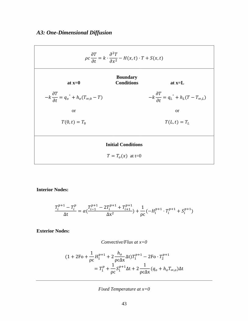
Determination of Coefficients
Multiply the wave equation by
and integrate over the domain.
∫ ∫
∫ ∫
∫ ∫
∫ ∫
1st term:
∫ ∫
(
∫ ∫
)⏟
2nd
term:
∫ ∫
3rd
term:
∫ ∫
∫
[(
)
(
)
(
)
(
)
∫
]
- , (
)
(
)
, (
)
, (
)
∫
∫
⏟
48
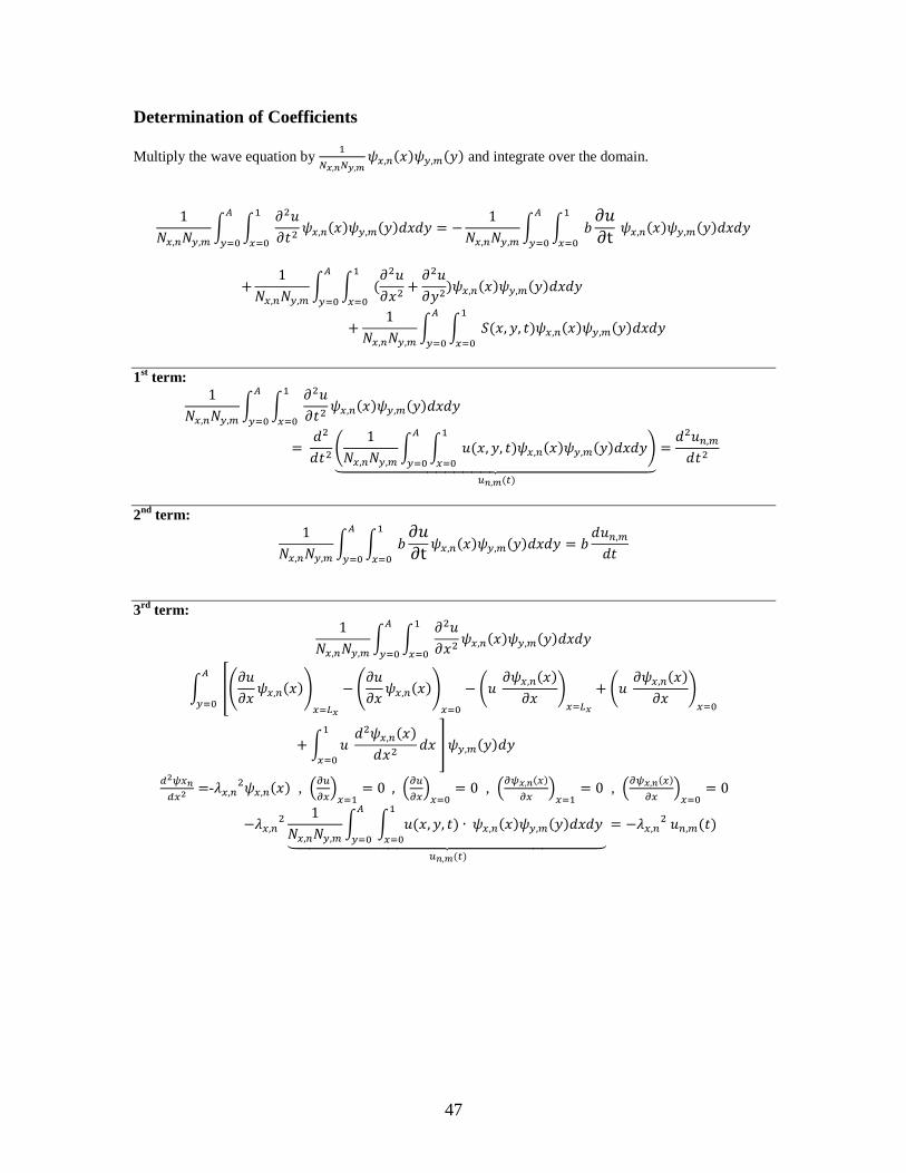
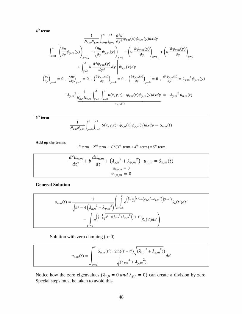
4th
term:
∫ ∫
∫
[(
)
(
)
(
)
(
)
∫
]
(
)
, (
)
, (
)
, (
)
,
-
∫
∫
⏟
5th
term
∫ ∫
Add up the terms:
1st term + 2
nd term + (3
rd term + 4
th term) = 5
th term
(
)
General Solution
√ (
)
( ∫ (
√ (
))
∫ (
√ (
))
)
Solution with zero damping (b=0)
∫ √
√
Notice how the zero eigenvalues ( can create a division by zero.
Special steps must be taken to avoid this.

49
Appendix B
Mathematica Source Code
B1: Numerical Integration
fN1[x_,c1_,c2_,c3_]:=c1+c2*x+c3*x2;
fN2[x_,c1_,c2_,c3_]:=c1+c2*Sin[c3*2*x];
fN3[x_,c1_,c2_,c3_]:=c1+c2*Exp[c3*x];
NumericalIntegration[rule_,segments_,bN1_,aN1_,fNum_,c1N1_,
c2N1_,c3N1_]:=Module[{n,x,xdata,fdata,xfdata,error,Irule,I
exact},
fN1[x_,c1_,c2_,c3_]:=c1+c2*x+c3*x2;
fN2[x_,c1_,c2_,c3_]:=c1+c2*Sin[c3*2*x];
fN3[x_,c1_,c2_,c3_]:=c1+c2*Exp[c3*x];
n=1+rule*segments;
x=(bN1-aN1)/(n-1);
xdata=aN1+x*Range[0,n-1]; fdata=fNum[xdata,c1N1,c2N1,c3N1];
xfdata=Transpose[{xdata,fdata}];
Irule=Round[Sum[
Integrate[
Interpolation[
xfdata[[1+(i-1)*rule;;1+i*rule]],
InterpolationOrderrule][x],
{x,xdata[[1+(i-1)*rule]],xdata[[1+i*rule]]}],
{i,1,segments}],.001];
Iexact=Round[Integrate[fNum[x,c1N1,c2N1,c3N1],{x,aN1,bN1}],
.001];
error=If[Iexact0,Round[Irule-Iexact,0.01],Round[Abs[(Irule-Iexact)/Iexact]*100,0.01]];
Show[{
Table[
Plot[
Interpolation[
xfdata[[1+(i-1)*rule;;1+i*rule]],
InterpolationOrderrule][x],
{x,xdata[[1+(i-1)*rule]],xdata[[1+i*rule]]},
PlotRangeAll,
PlotStyle{Dashed,Thick,Blue},

50
Filling0,
FillingStyleIf[OddQ[i],LightBlue,Opacity[0.2,Blue]]
],
{i,1,segments}
],
Table[
ListPlot[
{xfdata[[i]]},
PlotRangeAll,
PlotMarkers{,9},
Filling0,
FillingStyleIf[IntegerQ[(i-
1)/rule],{{Thin,Blue}},{{Dashed,Thin,Blue}}]
],
{i,1,n}
],
Plot[fNum[x,c1N1,c2N1,c3N1],{x,aN1,bN1},
PlotRangeAll,
PlotStyle{Thick,Black}
]
},
ImageSize400,
Ticks{{aN1,bN1},All},
AxesOrigin{aN1-(bN1-aN1)/10,0},
AxesLabel{Style["x",14],Style["f(x)",14]},
PlotLabel
Column[{
Style[Row[{"I = ",Iexact}],14],
Style[If[
Iexact0, Row[{ "abs error = ",error }],
Row[ {"error = ",error ,"%"}]
],14]
},Center]
]
]
Manipulate[
NumericalIntegration[rule,segments,bN1,aN1,fNum,c1N1,c2N1,c
3N1],
{{rule,2,"integration rule"},{1"Trapezoid: 1st
order",2"Simpson's 1/3: 2nd order",3"Simpson's 3/8: 3
rd
51
order",4"Boole's: 4th order",5"5
th order",6"6
th
order"},ControlTypePopupMenu},
{{segments,3,"segments"},1,16,1,Appearance"Labeled"},
Delimiter,
{{fNum,fN2,"function"},{fN1"polynomial: f(x) =
c1+c2·x+c3·x2",fN2"oscillator: f(x) =
c1+c2·sin(c3·2·x)",fN3"exponential: f(x) = c1+c2·
"},ControlTypePopupMenu},
{{c1N1,0,"c1"},-4,4,.1,Appearance"Labeled"},
{{c2N1,1,"c2"},-4,4,.1,Appearance"Labeled"},
{{c3N1,-2.2,"c3"},-4,4,.1,Appearance"Labeled"},
Delimiter,
{{aN1,0,"lower limit, a"},-1,bN1-
0.1,0.1,Appearance"Labeled"},
{{bN1,1,"upper limit,
b"},aN1+0.1,1,0.1,Appearance"Labeled"},
SaveDefinitionsTrue,
ControlPlacementTop]
B2: Discrete Green’s Function and Duhamel’s Methods
SC[1][t_,p_]:=UnitStep[t-0]-UnitStep[t-p];
SC[2][t_,p_]:=Cos[p*t]*UnitStep[t];
xexact[1][tmax_,a_,S_,p_]:=NDSolve[{x'[t]+a*x[t]S[t,p],x[0
]0},x,{t,0,tmax}];
xexact[2][tmax_,a_,S_,p_]:=NDSolve[{x''[t]+a^2*x[t]S[t,p],
x[0]0,x'[0]0},x,{t,0,tmax}];
[1][1][t_,to_,t_,a_]:=1/a (1--a (t-to))UnitStep[t-to]-
1/a (1--a (t-to-t))UnitStep[t-to-t];
[2][1][t_,to_,t_,a_]:=1/a (1--a (t-to))UnitStep[t-to];
[1][2][t_,to_,t_,a_]:= 1/a2 (1-Cos[a *(t-to)])UnitStep[t-
to]- 1/a2 (1-Cos[a *(t-to-t)])UnitStep[t-to-t];
[2][2][t_,to_,t_,a_]:= 1/a2 (1-Cos[a *(t-to)])UnitStep[t-
to];
c3 x

52
xapprox[1][ode_][t_,to_,t_,a_,S_,p_]:=S[to,p]*[1][ode][t,
to,t,a];
xapprox[2][ode_][t_,to_,t_,a_,S_,p_]:=(S[to,p]-S[to-
t,p])*[2][ode][t,to,t,a];
SourcePlot=
Show[{
Plot[
Evaluate[
{S[source][t,p],
sdata.(UnitStep[t-tdata]-UnitStep[t-tdata-t])}
],
{t,0,tmax},
PlotStyle{{{Red,Thick}},{Black,Dashed,Thickness[0.012]}},
Filling{10},
FillingStyleOpacity[.1,Red],
PlotRangeAll,
ExclusionsNone],
If[method1,
ListPlot[stdata,
Filling0,
FillingStyle{Black,Dashed,Thin}
],
Table[
ListLinePlot[{
{tdata[[n]],sdata[[n]]},{tmax,sdata[[n]]} },
PlotStyle{Black,Dashed,Thin}],
{n,segments}]
]},
PlotRangeAll,
AxesOrigin{0,0},
PlotLabelStyle["source",14],
AxesLabel{Style["t",14, Italic],Style["S(t)",14,
Italic]}
];
ResponsePlot=
Show[{
Plot[
Evaluate[x[t]/.xexact[ode][tmax,a,SC[source],p]],
{t,0,tmax},
PlotStyle{{Red,Thick}},
Filling0,

53
FillingStyleOpacity[.1,Red],
ExclusionsNone,
PlotRangeAll],
Plot[
Evaluate[Total[xapprox[method][ode][t,tdata,t,a,SC[source]
,p]]],
{t,0,tmax},
PlotStyle{Black,Dashed,Thickness[0.012]},
ExclusionsNone,
PlotRangeAll],
Plot[
Evaluate[xapprox[method][ode][t,tdata,t,a,SC[source],p]], {t,0,tmax},
PlotStyle{{Black,Dashed,Thin}},
PlotRangeAll,
ExclusionsNone]
},
AxesOrigin{0,0},
PlotLabelStyle["response",14],
AxesLabel{Style["t",14, Italic],Style["x(t)",14,
Italic]}
];
GraphicsColumn[{
SourcePlot,
ResponsePlot}]
]
Manipulate[
LinearityPlots[{methodC,segmentsC},{ode,aC,tmaxC},{source,p
C}],
{{ode,1,"ODE"},{
1Row[{"first order:
",Row[{Style["d",Italic],Style["x",Italic]}]/Row[{Style["d"
,Italic],Style["t",Italic]}]," + ",Style["a",Italic],"
",Style["x",Italic]," =
",Style["S",Italic],"(",Style["t",Italic],")"}],
2Row[{"second order:
",Row[{Style["d",Italic]2,Style["x",Italic]}]/Row[{Style["d"
,Italic],Style["t",Italic]2}]," + ",Style["a",Italic]
2,"
",Style["x",Italic]," =
",Style["S",Italic],"(",Style["t",Italic],")"}]},
ControlTypePopupMenu,MenuStyle"TR"},

54
{{aC,1, Row[{"parameter
",Style["a",Italic]}]},.01,5,Appearance"Labeled"},
{{tmaxC,1,"max time"},1,10,Appearance"Labeled"},
Delimiter,
{{methodC,1,"method"},{1"pulses: Green's
function",2"strips: Duhamel's"}},
{{segmentsC,4,"segments"},1,16,1,Appearance"Labeled"},
Delimiter,
{{source,2,"source"},{1Row[{"pulsed:
UnitStep(",Style["t",Italic],")-
UnitStep(",Style["t",Italic],"-
",Style["p",Italic],")"}],2Row[{"harmonic:
cos(",Style["p",Italic],"
",Style["t",Italic],")"}]},ControlTypePopupMenu,MenuStyle
"TR"},
{{pC,/2, Row[{"parameter
",Style["p",Italic]}]},0,10,Appearance"Labeled"},
ControlPlacementLeft,
SaveDefinitionsTrue,
AutorunSequencing{{5,10},4,1,6}
]

55
B3: Dynamics of Chaotic Maps
f[1][x_,r_]:=r*x(1-x)
f[2][x_,r_]:=x^2+r
SetOptions[{ListPlot,ListLinePlot,Plot},ImageSize250,AxesO
rigin{0,0}];
a=.007;
FinalStatePlots[1]=
Show[
{ListPlot[
Transpose[Table[Drop[NestList[f[1][#,r]&,.1,175],150],{r,3.
45,4,a}]],
PlotStyle{{AbsolutePointSize[0.01],Gray}},
DataRange->{3.45,4}],
Plot[(-1+r)/r,{r,1,3},PlotStyleGray,
PlotRange{0,1}],
Plot[{(r+r2-r )/(2 r
2),(r+r
2+r )/(2
r2)},{r,3,3.45},PlotStyleGray]},
AxesLabel{Style["r",Bold,10],Style["x*",Bold,10]},
PlotLabelStyle["Final State Diagram",Bold,12],
AxesOrigin{0,0},
PlotRange{{0,4},{-.05,1.05}}];
FinalStatePlots[2]=Show[{
ListPlot[
Transpose[Table[Drop[NestList[#^2+r&,.1,175],150],{r,-
2,-1.25,a}]],
PlotStyle{{AbsolutePointSize[0.01],Gray}},
DataRange->{-2,-1.25}],
Plot[{1/2 (-1- ),1/2 (-1+ )},{c,-.75,-
1.25},PlotStyleGray],
Plot[1/2 (1- ),{c,-.75,.25},PlotStyleGray]},
AxesLabel{Style["r",Bold,10],Style["x*",Bold,10]},
PlotLabelStyle["Final State Diagram",Bold,12],
PlotRangeAll];
LyapunovFunc[eqn_][r_,xo_,n_]:=1/(n+1)
Plus@@(Log[Abs[D[f[eqn][x,r],x]/.x#1]]&/@NestList[f[eqn][x
,r]/.x#1&,xo,n])
LyapunovExpPlots[1]=Plot[LyapunovFunc[1][r,.1,90],{r,0,4},
3 2 r r2 3 2 r r2
3 4 c 3 4 c
1 4 c

56
PlotStyleBlack,
PlotRange{{0,4},{-1.5,.7}},
AxesLabel{Style["r",Bold,10],Style["",Bold,10]},
PlotLabelStyle["Lyapunov Exponent",Bold,12]];
LyapunovExpPlots[2]=Plot[LyapunovFunc[2][r,.1,90],{r,-
2,.25},
PlotStyleBlack,
PlotRange{{-2,.25},{-1.5,.7}},
AxesLabel{Style["r",Bold,10],Style["",Bold,10]},
PlotLabelStyle["Lyapunov Exponent",Bold,12]];
Manipulate[
Module[{pts,OrbitData,OrbitPlot,FinalStatePlot,CobwebPlot,L
yapunovPlot},
xo11={{xo1,xo2},{xo1-.5,xo2-.5}};
r11[1]:=4*r1;
r11[2]:=2.25*r1-2;
pts=x/.Solve[xf[eqn][x,r[eqn]],x];
OrbitData=Transpose[NestList[f[eqn][#,r11[eqn]]&,xo11[[eqn]
],100]];
OrbitPlot=Show[{
ListLinePlot[
Table[Transpose[{Range[0,n11,1],OrbitData[[i]][[1;;n11+1]]}
],{i,1,2,1}],
PlotRange{
If[n11<25,{-.5,25.5},{n11-25,n11+1}],Which[eqn1,{-
.05,1.05},eqn2,{-2.05,2.05}]},
MeshFull,
MeshStyle{PointSize[Medium],Gray},
PlotStyle{Blue,Red},
DataRange{0,n11},
AxesLabel{Style["i",Bold,10],Style["xi",Bold,10]}],
ListPlot[Table[{{n11,OrbitData[[i]][[n11+1]]}},{i,1,2,1}],
PlotStyle{{PointSize[Large],Blue},{PointSize[Large],Red}}]
},
PlotLabelStyle["Orbit",Bold,12],
AxesOriginIf[n11<25,{-.5,0},{n11-25,0}],
ImageSize250];
FinalStatePlot=Show[{
FinalStatePlots[eqn],
57
ListPlot[Table[{{r11[eqn],OrbitData[[p]][[n11+1]]}},{p,1,2,
1}],
PlotStyle{{PointSize[Large],Blue},{PointSize[Large],Red}}]
}];
CobwebPlot=Show[{
Plot[{f[eqn][x,r11[eqn]],x},{x,-2,2},
PlotStyle{{Black,Thick},{Black,Thick}},
AxesLabel{Style["xi-
1",Bold,10],Style["xi",Bold,10]}],
ListPlot[
Table[{pts[[i]],pts[[i]]},{i,1,Length[pts]}],
PlotStyle{Black,PointSize[Large]}],
ListLinePlot[
Table[
Table[{If[i0,OrbitData[[p]][[1]],OrbitData[[p]][[i]]],If[i
0,0,OrbitData[[p]][[i+1]]]},{i,0,n11}],
{p,1,2,1}],
InterpolationOrder0,
PlotStyle{{Blue},{Red}},
AxesOrigin{0,0}],
Table[ListPlot[{{OrbitData[[p]][[n11]],If[n110,0,OrbitData
[[p]][[n11+1]]]}},
PlotStyle{PointSize[Large],If[p1,Blue,Red]}],{p,1,2,1}]
},
PlotLabelStyle["Cobweb Diagram",Bold,12],
PlotRangeWhich[eqn1,{{0,1},{1,0}},eqn2,{{-2,2},{-2,2}}],
ImageSize250];
LyapunovPlot=Show[{
LyapunovExpPlots[eqn],
Graphics[{Dashed,Thick,Gray,Line[{{r11[eqn],2},{r11[eqn],-
3.5}}]}]}];
Deploy[
Grid[{{
OrbitPlot,
FinalStatePlot},
{CobwebPlot,
LyapunovPlot}},
FrameTrue]]],
58
Row[{
Column[{Control[{{eqn,1,""},{1Row[{Style["logistic
map",10,Bold],Spacer[10],Style[" SubscriptBox[x,\i] = r ·
SubscriptBox[x,\i-1](1 - SubscriptBox[x,\i-
1])",12,Italic]}],
2Row[{Style["quadratic
map",Bold,10],Spacer[10],Style[" SubscriptBox[x,\i] =
SuperscriptBox[SubscriptBox[x,\i-1],\2] +
r",12,Italic]}]},ControlTypePopupMenu}],
Row[{Control[{{n11,10,Style["time
steps",10,Italic]},0,60,1,ImageSizeSmall}],Spacer[5],Style
[Dynamic[n11],10]}]}],
Spacer[100],
Column[{Style["driving parameter",Bold,10],
Row[{Control[{{r1,.5,Style["r",12,Italic]},0,1,ImageSizeTi
ny}],Spacer[5],Style[Dynamic[r11[eqn]],10]}],
Style["initial conditions",Bold,10],
Row[{Control[{{xo1,.1,Row[{Style["SubscriptBox[x,\0]",Itali
c,10],Spacer[5],Style["",Blue,10]}]},0,1,ImageSizeTiny}],
Spacer[5],Style[Dynamic[xo11[[eqn,1]]],10],Spacer[5]}],
Row[{Control[{{xo2,.2,Row[{Style["SubscriptBox[x,\0]",Itali
c,10],Spacer[5],Style["",Red,10]}]},0,1,ImageSizeTiny}],S
pacer[5],Style[Dynamic[xo11[[eqn,2]]],10],Spacer[5]}]
},
ItemSize{15.75,1},
FrameTrue]}],
SaveDefinitionsTrue,
ControlPlacement{Top}]
B4: One-Dimensional Diffusion
Lx1=1;ii1=50;
c1=1;k1=1; S11=10;Sx11=0;Sx21=.3;
H11=15;Hx11=.8;Hx21=1;
BCx01=1;T01=0;q01=0;h01=0;T01=0;
BCxL1=2;TL1=0;qL1=0;hL1=0;TL1=0;

59
Tinit11=2;Tinitx11=.25;Tinitx21=.75;
t1=.01;n11=1;
pmaxFD=100;
Temperature1D[
{Lx1_,ii1_},
{c1_,k1_},
{S11_,Sx11_,Sx21_},
{H11_,Hx11_,Hx21_},
{BCx01_,T01_,q01_,h01_,T01_},
{BCxL1_,TL1_,qL1_,hL1_,TL1_}, {Tinit11_,Tinitx11_,Tinitx21_},
{t1_,pmax1_}]:=
Module[{x1,1,Fo1,x1,upperDiag1,lowerDiag1,diag01,p1,Tinit
ial1,diag1,rhs1,coeff1},
x1=Lx1/(ii1-1);
1=k1/c1;
Fo1=(1*t1)/x12;
x1=Table[(i-1)*x1,{i,1,ii1}]; upperDiag1=-Fo1*Table[1,{ii1-1}];
lowerDiag1=upperDiag1;
diag01=(1+2*Fo1)Table[1,{ii1}];
p1=1;
Tinitial1=Tinit11*(UnitStep[x1-Tinitx11]-UnitStep[x1-
Tinitx21]);
NestList[
Module[
{},
diag1=diag01+1/c1 H11*(UnitStep[x1-Hx11]-UnitStep[x1-
Hx21])*t1;
rhs1=#+1/c1 S11*(UnitStep[x1-Sx11]-UnitStep[x1-
Sx21])*t1;
Which[
BCx01 1,
upperDiag1[[1]]=0;
diag1[[1]]=1.;
rhs1[[1]]=T01,
BCx01 2,

60
upperDiag1[[1]]=-2*Fo1;
diag1[[1]]=diag1[[1]]+2 1/(c1*x1) h01*t1 ;
rhs1[[1]]=rhs1[[1]]+2 1/(c1*x1) (q01+h01*T01)*t1 ];
Which[
BCxL1 1,
lowerDiag1[[ii1-1]]=0;
diag1[[ii1]]=1.;
rhs1[[ii1]]=TL1,
BCxL1 2, lowerDiag1[[ii1-1]]=-2*Fo1;
diag1[[ii1]]=diag1[[ii1]]+2 1/(c1*x1) hL1*t1;
rhs1[[ii1]]=rhs1[[ii1]]+2 1/(c1*x1)
(qL1+hL1*TL1)*t1 ];
coeff1=
SparseArray[
{Band[{1,2}]upperDiag1,
Band[{1,1}]diag1,
Band[{2,1}]lowerDiag1},
ii1];
LinearSolve[coeff1,rhs1]
]&,
Tinitial1,pmax1]]
Column[{
Dynamic@Deploy[Grid[{{
Column[{
Row[{"t=
",InputField[Dynamic[t1],Number,FieldSizeTiny]," s"}]
},AlignmentCenter],
Column[{
Row[{"Lx=
",InputField[Dynamic[Lx1],Number,FieldSizeTiny]," m"}],
Row[{"ii=
",Slider[Dynamic[ii1],{3,101,1},ImageSizeSmall,ContinuousA
ctionFalse]," ",Dynamic[ii1]}]},AlignmentCenter],
Column[{
Row[{"c=
",InputField[Dynamic[c1],Number,FieldSizeTiny],"
kJ/(m3·K)"}],

61
Row[{"k=
",InputField[Dynamic[k1],Number,FieldSizeTiny],"
W/(m·K)"}]
}]
},
{Column[{
Row[{Style["Boundary Condition",Bold]}],
Row[{Style["at x=0",Bold]}],
"",
Control[{BCx01,{1"constant
temp",2"convection,flux"},ControlTypeSetter,Appearance"
Vertical"}],"",
Which[
BCx011,
Row[{"T0=",InputField[Dynamic[T01],Number,FieldSizeTiny],"
K"}],
BCx012,
Column[{
Row[{"h0=
",InputField[Dynamic[h01],Number,FieldSizeTiny],"
W/(m2·K)"}],
Row[{"q0=
",InputField[Dynamic[q01],Number,FieldSizeTiny]," W"}],
Row[{"T=
",InputField[Dynamic[T01],Number,FieldSizeTiny]," K"}]
}]]
},AlignmentCenter
],
Temp=Temperature1D[{Lx1,ii1},
{c1,k1}, {S11,Sx11*Lx1,Sx21*Lx1},
{H11,Hx11*Lx1,Hx21*Lx1},
{BCx01,T01,q01,h01,T01},
{BCxL1,TL1,qL1,hL1,TL1},
{Tinit11,Tinitx11*Lx1,Tinitx21*Lx1},
{t1,pmaxFD}];
Column[{
Row[{Style["VIRGINIA TECH",14,Bold,Orange]}],
"",
Row[{Style["Mechanical
Engineering",14,Bold,Darker[RGBColor[1,0,0],.4]]}],
"",
Row[{Style["Finite Difference
Solutions",10,Bold]}],

62
Row[{Style["to 1D Diffusion Equation",10,Bold]}]
},Center],
Column[{
Row[{Style["Boundary Condition",Bold]}],
Row[{Style[" at x=L",Bold]}],
"",
Control[{BCxL1,{1"constant
Temp",2"convection,flux"},ControlTypeSetter,Appearance"
Vertical"}],"",
Which[
BCxL11,
Row[{"TL=
",InputField[Dynamic[TL1],Number,FieldSizeTiny]," K"}],
BCxL12, Column[{
Row[{"hL=
",InputField[Dynamic[hL1],Number,FieldSizeTiny],"
W/(m2·K)"}],
Row[{"qL=
",InputField[Dynamic[qL1],Number,FieldSizeTiny]," W"}],
Row[{"T=
",InputField[Dynamic[TL1],Number,FieldSizeTiny]," K"}]
}]]
},AlignmentCenter]},
{
Column[{
Row[{"",Style["Volumetric Sources,
S(x)",Bold,BackgroundOpacity[.1,Red]]}],
Row[{"So=
",InputField[Dynamic[S11],Number,FieldSizeTiny]," W/m3"}],
Row[{"So,x1= ",Slider[Dynamic[Sx11],{0,Sx21-
.05,.05},ContinuousActionFalse,
ImageSizeTiny],Spacer[5],Dynamic[Sx11],"%"}],
Row[{"So,x2=
",Slider[Dynamic[Sx21],{Sx11+.05,1,.05},ContinuousActionFa
lse, ImageSizeTiny],Spacer[5],Dynamic[Sx21],"%"}]},
AlignmentLeft,
ItemSize15],
Column[{
Row[{Style["Initial
Temperature",Bold,BackgroundOpacity[.1,Blue]]}],
Row[{Style["Distribution,
To(x)",Bold,BackgroundOpacity[.1,Blue]]}],

63
Row[{Style["To=
",12],InputField[Dynamic[Tinit11],Number,FieldSizeTiny],"
K"}],
Row[{"To,x1=
",Slider[Dynamic[Tinitx11],{0,Tinitx21-
.05,.05},ContinuousActionFalse,
ImageSizeTiny],Spacer[5],Dynamic[Tinitx11],"%"}],
Row[{"To,x2=
",Slider[Dynamic[Tinitx21],{Tinitx11+.05,1,.05},ContinuousA
ctionFalse,
ImageSizeTiny],Spacer[5],Dynamic[Tinitx21],"%"}]},
AlignmentCenter],
Column[{
Row[{Style["Proportional Losses,
H(x)",12,Bold,BackgroundOpacity[.1,Green]]}],
Row[{"Ho=
",InputField[Dynamic[H11],Number,FieldSizeTiny],"
W/(m3·K)"}],
Row[{"Ho,x1= ",Slider[Dynamic[Hx11],{0,Hx21-
.05,.05},ContinuousActionFalse,
ImageSizeTiny],Spacer[5],Dynamic[Hx11],"%"}],
Row[{"Ho,x2=
",Slider[Dynamic[Hx21],{Hx11+.05,1,.05},ContinuousActionFa
lse, ImageSizeTiny],Spacer[5],Dynamic[Hx21],"%"}]},
AlignmentLeft,
ItemSize15]
}},Frame{True,All,{{2,0}True}},
BackgroundWhite]],
Manipulate[
If[nFD>pmax1,nFD=pmax1];
Show[{
ListLinePlot[
Temp[[nFD]],
AxesLabel{"x","T"},
PlotStyle{Thickness[0.005]},
PlotRangeAll,
DataRange{0,Lx1},
Filling0,
ImageSize500,
FrameTrue,
FrameTicks{{All,None},{{0,Lx1/2,Lx1},None}},
FrameLabel{"x","T"}

64
],
Plot[.5*Max[Temp]*(UnitStep[x1FD-Sx11*Lx1]-
UnitStep[x1FD-Sx21*Lx1]),{x1FD,0,Lx1},
Filling0,
FillingStyleOpacity[.1,Red],
PlotStyleOpacity[.1,Red]],
Plot[.5*Max[Temp]*(UnitStep[x1FD-Hx11*Lx1]-
UnitStep[x1FD-Hx21*Lx1]),{x1FD,0,Lx1},
Filling0,
FillingStyleOpacity[.1,Green],
PlotStyleOpacity[.1,Green]]
},
PlotLabelRow[{"time = " ,t1*n11," sec"}],
AxesOrigin{0,0},
PlotRange{Max[Temp],Min[Temp]},
ImageSize300
]
,
{{nFD,5,"time steps,
p"},1,pmax1,1,Appearance"Labeled"},
{{pmaxFD,20,"pmax"},10,200,10,Appearance"Labeled",Continuo
usActionFalse},
LocalizeVariablesFalse,
SaveDefinitionsTrue]},
Center]
B5: Wave Mechanics
terms=20;
x[1]=N[Table[n ,{n,1,terms}]];
y[1]=N[Table[(m )/A,{m,1,terms}]];
2[1]=Table[x[1][[m]]2+y[1][[n]]2,{m,1,terms},{n,1,terms}]
;
x[2]=N[Table[n ,{n,0,terms-1}]];
y[2]=N[Table[(m )/A,{m,0,terms-1}]];
2[2]=Table[x[2][[m]]2+y[2][[n]]2,{m,1,terms},{n,1,terms}]
;
x[1]=Sin[x[1]*x];

65
y[1]=Sin[y[1]*y];
[1]=Transpose[{x[1]}].{y[1]};
x[2]=Cos[x[2]*x];
y[2]=Cos[y[2]*y];
[2]=Transpose[{x[2]}].{y[2]};
Nx[1]=Table[1/2,{i,1,terms}];
Ny[1]=Table[A/2,{i,1,terms}];
Nx[2]=Prepend[Table[1/2,{i,1,terms-1}],1];
Ny[2]=Prepend[Table[A/2,{i,1,terms-1}],A];
xint[1]=1/Nx[1]
(Integrate[Sin[lam*x],{x,xstart,xend}]/.lamx[1]);
yint[1]=1/Ny[1]
(Integrate[Sin[lam*y],{y,ystart,yend}]/.lamy[1]);
int[1]=Transpose[{xint[1]}].{yint[1]};
xint[2]=1/Nx[2]
Prepend[Integrate[Cos[lam*x],{x,xstart,xend}]/.lamx[2][[2
;;terms]],(xend-xstart)];
yint[2]=1/Ny[2]
Prepend[Integrate[Cos[lam*y],{y,ystart,yend}]/.lamy[2][[2;;terms]],(yend-ystart)];
int[2]=Transpose[{xint[2]}].{yint[2]};
Eint[1]=2*Exp[-B*t/2]*Sin[t/2* ]/ ;
Eint[2]=2*Exp[-B*t/2]*Sin[t/2* ]/ ;
Solution[1][x_,y_,t_,xstart_,ystart_,xend_,yend_,A_,B_]=Tot
al[Eint[1]*int[1]*[1],2];
Solution[2][x_,y_,t_,xstart_,ystart_,xend_,yend_,A_,B_]=Tot
al[Eint[2]*int[2]*[2],2];
Manipulate[
Plot3D[
Evaluate[
Solution[BC][x,y,t,Spts[[1]]-.05,Spts[[2]]-
.05,Spts[[1]]+.05,Spts[[2]]+.05,A,B]
],
{x,0,1},{y,0,A},
4 2 1 B2
4 2 1 B2
4 2 2 B2
4 2 2 B2

66
PlotRange0.05{-1,1},
BoxRatios{1,A,5/8},
PlotPointsControlActive[30,50],
MaxRecursion2,
BoxedFalse,
MeshNone,
AxesFalse],
{{t,0,"time\n"},0,2* ,0.01,Appearance"Labeled"},
{{BC,1,"boundaries\n"},{1" fixed ",2" free "}},
{{A,1,"aspect ratio\n"},.1,1,Appearance"Labeled"},
{{B,0.001,"damping\n"},0.001,2,Appearance"Labeled"},
{{Spts,{.5,.5},"source point "},{.05,.05},{.95,A-
.05},ControlTypeSlider2D},
ControlPlacement{Top,Top,Top,Top,Left},
SaveDefinitionsTrue]
2