a dynamic inequality generation scheme for polynomial ... · a dynamic inequality generation scheme...

Noname manuscript No.(will be inserted by the editor)

A Dynamic Inequality Generation Scheme for Polynomial Programming

Bissan Ghaddar · Juan C. Vera · Miguel F. Anjos

Received: date / Accepted: date

Abstract Hierarchies of semidefinite programs have been used to approximate or even solve polynomial pro-grams. This approach rapidly becomes computationally expensive and is often tractable only for problemsof small size. In this paper, we propose a dynamic inequality generation scheme to generate valid polyno-mial inequalities for general polynomial programs. When used iteratively, this scheme improves the boundswithout incurring an exponential growth in the size of the relaxation. As a result, the proposed scheme is inprinciple scalable to large general polynomial programming problems. When all the variables of the problemare non-negative or when all the variables are binary, the general algorithm is specialized to a more efficientalgorithm. In the case of binary polynomial programs, we show special cases for which the proposed schemeconverges to the global optimal solution. We also present several examples illustrating the computational be-havior of the scheme and provide comparisons with Lasserre’s approach and, for the binary linear case, withthe lift-and-project method of Balas, Ceria, and Cornuejols.

Keywords Polynomial programming · Binary polynomial programming · Semidefinite programming ·Inequality generation

1 Introduction

A polynomial program is a mathematical optimization problem whose objective and constraints are multivari-ate polynomials. Polynomial programming generalizes several special cases that have been thoroughly studiedin optimization, including mixed binary linear programming, convex and non-convex quadratic programming,and linear complementarity problems. Polynomial programs arise in several practical applications in the con-text of control, process engineering, facility location, economics and equilibrium, and finance. It is well knownthat solving polynomial programs is an NP-hard problem.

Since the work of Lasserre [15] and Parrilo [25], there has been a lot of research activity to devise solutionschemes to solve polynomial programs. These schemes are based on applying representation theorems fromalgebraic geometry to characterize the set of polynomials that are non-negative on a given domain. This researchincludes the recent work of de Klerk and Pasechnik [5], Lasserre [14,15], Laurent [17,18], Nie, Demmel, andSturmfels [22], Parrilo [23,25], Pena, Vera, and Zuluaga [28,36], and the early work of Nesterov [20], Shor [34],and the S−Lemma of Yakubovich (see [30]) among others. The recent handbook [1] provides an overview ofthe research activity in the area of polynomial programming.

An extended abstract version of this paper has appeared in the Proceedings of IPCO 2011.

B. GhaddarIBM Research, Dublin Technology Campus,Damastown Ind. Park, Mulhuddart, Dublin 15, Ireland.Research supported by a Canada Graduate Scholarship from the Natural Sciences and Engineering Research Council of Canada.E-mail: [email protected]

J. C. VeraTilburg School of Economics and Management, Tilburg University,Tilburg, The Netherlands.E-mail: [email protected]

M. F. AnjosCanada Research Chair in Discrete Nonlinear Optimization in Engineering, GERAD & Ecole Polytechnique de Montreal,Montreal, QC, Canada H3C 3A7.Research partially supported by the Natural Sciences and Engineering Research Council of Canada, and by a HumboldtResearch Fellowship.E-mail: [email protected]

2 B. Ghaddar, J.C. Vera, and M.F. Anjos

The general approach to solve polynomial programs is based on sum-of-squares (SOS) certificates of non-negativity for multivariate polynomials. This approach builds hierarchies of relaxations leading to solvinga sequence of positive semidefinite programs. Under mild conditions, the resulting semidefinite relaxationsprovide bounds that converge to the optimal value of the original polynomial program. Allowing for morecomplex certificates produces better approximations to the original polynomial program, but the size of suchapproximations explodes quickly, even for instances with a small number of variables. As a result, despite thetheoretical strength of SOS representations, the current schemes are only able to handle problems of smallsizes. For efficient practical performance in medium or large-scale problems, it becomes necessary to exploitthe problem structure. For example, by taking advantage of the symmetry such as the work of Bai, de Klerk,Pasechnik, and Sotirov [2], de Klerk [4], de Klerk, Pasechnik, and Schrijver [6], de Klerk and Sotirov [7], andGatermann and Parrilo [10] or by exploiting sparsity such as in Kim, Kojima, and Toint [13] and Nie andDemmel [21] and the references therein. However, in the absence of structure, the practical application of theSOS approach is severely limited.

In this paper, a dynamic inequality generation scheme (DIGS) is proposed for general polynomial pro-grams. The key idea of DIGS is to bound the complexity (degree) of the non-negative certificates, avoidingthe exponential growth of the relaxations. Instead, our approach makes use of information from the objectivefunction to construct improved approximations of the polynomial program, by dynamically generating poly-nomial inequalities that are valid on the feasible region. These valid inequalities are used to construct newnon-negative certificates. The iterated generation of inequalities yields better and better approximations tothe polynomial program without growing the degree of the certificates involved. Depending on the originalproblem and the type of relaxation used, the iterative procedure solves a sequence of linear, second-order cone,or semidefinite problems. For the purposes of this paper, we focus on semidefinite relaxations and thus obtaina sequence of semidefinite problems.

In the rest of this section we discuss Lasserre’s Hierarchy for Polynomial Programs. In Section 2 weintroduce our generic master-subproblem dynamic inequality generation scheme (Algorithm 1). Algorithm 1is a rather abstract scheme where the subproblem is not completely specified. In the rest of the paper wefocus on the specification of the subproblem. In Section 2.1, a practical algorithm for general PolynomialPrograms is presented (Algorithm 2). In the presence of extra structure, the subproblem can be implementedmore efficiently; this is done in Section 2.2 for Polynomial Programs where all variables are non-negative andin Section 3 where (some of) the variables are binary; we refer to such problems as (mixed) binary polynomialprograms (BPP). The method presented in Section 3 for the binary case can be seen as a generalization, frombinary linear programs to BPPs, of the lift-and-project methods of Balas, Ceria, and Cornuejols [3], Sherali andAdams [32], and Lovasz and Schrijver [19] (see Section 3.3). Our practical methods do not necessarily convergeto the optimal solution (see Example 5). The motivation for developing such methods is that, independentlyof the structure of the problem, they can efficiently strengthen the bounds which is helpful when incorporatedinto a branch-and-bound framework. Similar to the lift-and-project methods, these techniques can then beintegrated in the design of algorithms and solvers to efficiently solve polynomial programming problems.Convergence to the global optimal solution is proven for a family of problems in the binary case (Theorems1, 2 and 3). This specialized scheme and the convergence results are presented in Section 3. To evaluatethe proposed approach, computational results are presented for general polynomial programs (Section 2.1.2),non-negative polynomial programs (Section 2.2.1) and binary polynomial programs (Section 3.4); in each casewe compare our methodology to Lasserre’s approach [14,15]. For the binary linear case, we compare ourmethodology to the lift-and-project method of Balas, Ceria, and Cornuejols [3] (Section 3.3).

1.1 Polynomial Programming

Consider the general polynomial programming (PP) problem whose objective and constraints are multivariatepolynomials:

(PP-P) ρ = infx

f(x)

s.t. gi(x) ≥ 0, i = 1, . . . ,m.

When it is convenient, we represent a polynomial f(x) of degree deg(f) = d using use multinomial notation,i.e., we write f(x) =

∑|α|≤d fαx

α, where α = (α1, . . . αn) ∈ Nn, |α| =∑ni αi. We use R[x] := R[x1, . . . , xn]

(resp. Rd[x]) to denote the set of polynomials in n variables with real coefficients (resp. of degree at most d).

Let S = {x ∈ Rn : gi(x) ≥ 0, i = 1, . . . ,m} be the feasible set of (PP-P). Then (PP-P) can be rephrased as

supλλ

s.t. f(x)− λ ≥ 0 ∀ x ∈ S,

DIGS for Polynomial Programming 3

that is,

(PP-D) supλλ

s.t. f(x)− λ ∈ Pd(S),

where d is the maximum among deg(f(x)) and deg(gi(x)), i = 1, . . . ,m, and P(S) (resp. Pd(S)) is the coneof polynomials (resp. of degree at most d) that are non-negative over S ⊆ Rn. We refer to d as the degree of(PP-P).

The condition f(x) − λ ∈ Pd(S) is NP-hard for most (interesting) choices of S and d ≥ 1. Computablerelaxations of (PP-D) are obtained using tractable approximations of the cone Pd(S) which can be re-phrasedin terms of a linear system of equations involving positive semidefinite matrices [15,20,24–26,34,35], second-order cones [12], or linear optimization problems [16,33,36]. These approximations can be solved efficientlyusing interior-point methods.

The general idea in these methods is to relax the condition f(x)− λ ∈ Pd(S) to f(x)− λ ∈ K for a suitableK ⊆ Pd(S). Defining the relaxation

µK = supλλ

s.t. f(x)− λ ∈ K,

it follows that µK is a lower bound on the original problem (PP-P).

1.2 Lasserre’s Hierarchy for Polynomial Programs

Lasserre [15] introduced semidefinite relaxations corresponding to liftings of the polynomial programs intohigher dimensions. The construction is motivated by results related to representations of non-negative poly-nomials as SOS and the dual theory of moments. Lasserre shows that computing the global minimum of f(x)over a set S defined by polynomial inequalities reduces to solving a sequence of SOS-type representations ofpolynomials that are non-negative on S. The convergence of Lasserre’s method is based on the assumption that{g1(x), . . . , gm(x)}, the given description of S, allows the application of Putinar’s Theorem [31]. In particular,it assumes S is compact.

For ease of notation let g0(x) ≡ 1 and G = {gi(x) : i = 0, 1, . . . ,m}. For a given r > 0, let KrG be the r−thtruncated quadratic module generated by G, that is,

KrG =m∑i=0

gi(x)Σr−deg(gi),

where for any d ≥ 0, Σr denotes the cone of real polynomials of degree at most d that are SOS. Note thatΣd := {

∑Ni=1 pi(x)2 : p(x) ∈ Rb d

2c[x]}, with N = (n+dd ), and in particular Σd = Σd−1 for every odd degree d.

As KrG ⊆ P(S), we obtain a relaxation of (PP-D):

µrG = supλλ

s.t. f(x)− λ ∈ KrG,

so that µrG ≤ ρ and

µrG = supλ,σi(x)

λ

s.t. f(x)− λ =m∑i=0

gi(x)σi(x) (1)

σi(x) ∈ Σr−deg(gi), i = 0, . . . ,m.

The optimization problem (1) can be reformulated as a (convex) semidefinite optimization problem [34]. Byincreasing r, a sequence of semidefinite relaxations of increasing size is obtained. Lasserre shows [15] that undermild conditions, the optimal values of these relaxations converge to the global optimal value of the originalnon-convex problem (PP-P). Proposition 1 states the result using our notation.

Proposition 1 Let G = {gi(x) : i = 0, . . . ,m} be such that g0(x) ≡ 1. Assume there exists a real-valued polynomial

u(x) ∈∑mi=0 gi(x)Σm for some m, such that {x : u(x) ≥ 0} is compact. Then (Putinar [31])

K1G ⊆ K

2G ⊆ · · · ⊆ K

rG ⊆ · · · ⊆ P(S) and {p ∈ R[x] : p(s) > 0 ∀s ∈ S} ⊆

⋃r>0

KrG

and therefore (Lasserre [15])

µ1G ≤ µ2G ≤ · · · ≤ µ

rG ≤ · · · ≤ ρ and µrG → ρ as r →∞.


In other words, using Lasserre’s hierarchy for general polynomial programs one may approximate the globaloptimal value ρ as closely as desired by solving a sequence of semidefinite problems with increasing size ofthe semidefinite matrices and number of constraints. The computational cost of the procedure depends on r,the number of constraints m, and the number of variables n. For (PP-P) with n variables and m inequalityconstraints, the size of the optimization problem (1) is as follows:

– one psd matrix of size (n+rr );

– m psd matrices, each of size (n+r−deg(gi)r−deg(gi)

) for i = 1, . . . ,m;

– (n+rr ) linear constraints.

The number of constraints of (1) grows exponentially in r. Notice that to use all polynomial appearing in theformulation of (PP-P), r should be no smaller than d. When r > d+2, the number of variables and constraintsof (1) can be large, especially when (P-PP) involves high degree polynomials.

1.2.1 Equality Constraints

Lasserre’s approach treats equality constraints as pairs of two inequalities. Alternatively, one can differentiatebetween equality and inequality constraints as proposed in [28]. Given S = {x : gi(x) ≥ 0, i = 1, . . . ,m1, hi(x) =0, i = 1, . . . ,m2}, let G = {gi(x) : i = 0, 1, . . . ,m1, hi(x) : i = 1, . . . ,m2} where g0(x) = 1. Consider the followingapproximation of Pd(S):

KrG =

m1∑i=0

gi(x)Σr−deg(gi) +

m2∑i=1

hi(x)Rr−deg(hi)[x].

The corresponding optimization problem over S can be written as:

supλ,σi(x),δi(x)

λ

s.t. f(x)− λ =

m1∑i=0

σi(x)gi(x) +

m2∑i=1

δi(x)hi(x) (2)

σi(x) ∈ Σr−deg(gi), i = 0, . . . ,m1

δi(x) ∈ Rr−deg(hi)[x], i = 1, . . . ,m2.

In a similar way to problem (1), problem (2) can be reformulated as a semidefinite optimization problem.

2 Dynamic Approximation of Polynomial Programs

We propose a new scheme to generate a sequence of improving approximations for (P-PP). Instead of growingr and exponentially increasing the size of the relaxation (1), we fix r in (1) to a small value r0 (mainly tod, the degree of (PP-P)) and the relaxation (1) is improved by adding valid polynomial inequalities to thedescription of S, i.e., by growing the set G.

The scheme is dynamic, and consists of a master problem and a subproblem. The master problem is of theform (1) and provides bounds for problem (P-PP), while the subproblem uses the optimal dual information fromthe master to generate polynomial inequalities that are valid on the feasible region. These valid inequalities arethen incorporated into the master to construct new non-negativity certificates, obtaining better approximationsof (PP-P).

An augmented description G of S does not necessarily imply a better approximation. If p ∈ Kr0G , thenKr0G∪{p(x)} = Kr0G , and thus µr0G = µr0

G∪{p(x)}. On the other hand, if p(x) ≥ 0 is a valid inequality for S not

in Kr0G , we have Kr0G strictly contained in Kr0G∪{p(x)} improving the conic approximation to Pd(S) which may

provide a better bound for (PP-P) when using (1). We summarize this observation in Lemma 1.

Lemma 1 Let r0 ≥ d and p(x) ∈ Pr0(S) \ Kr0G . Then

Kr0G ( Kr0G∪{p(x)} ⊆ P(S) and thus µr0G ≤ µr0G∪{p(x)}.

We are interested in generating valid inequalities p(x) for which µr0G < µr0G∪{p(x)}. We call such inequalities

improving inequalities. Given a finite description G ⊆ Rd[x] for S and r0 ≥ d, Algorithm 1 is a generic dynamicinequality generation scheme (DIGS) based on Lemma 1 to construct a sequence of improving relaxations.


Algorithm 1 Generic Dynamic Inequality Generation Scheme (DIGS) for (PP-P)

Require: G ⊆ Rd[x] description of S and r0 ≥ ds← 0, G0 ← G.loop

Let

(PP-Ms) νs = supλ

λ

s.t. f(x)− λ ∈ Kr0Gs.

Look for an improving inequality ps(x) ∈ Pr0 (S) \ Kr0Gif an improving inequality does not exist then

STOPelseGs+1 ← Gs ∪ {ps(x)}s← s+ 1

end ifend loop

Lemma 1 implies that Algorithm 1 generates a sequence of strictly monotone approximations to Pd(S),and a corresponding sequence of improving bounds for the optimal value of (PP-P). This is formally stated inLemma 2.

Lemma 2 Let Gs and νs, s = 1, 2, . . . be generated by Algorithm 1. Then

Kr0G0( Kr0G1

( · · · ( Kr0Gs( Kr0Gs+1

· · · ⊆ P(S)

ν0 < · · · < νs < νs+1 < · · · ≤ ρ.

Moreover if Algorithm 1 stops at iteration s, then that bound is optimal, i.e., νs = ρ.

Proof By definition of improving inequality it follows that νs < νs+1 for all s. In particular Kr0Gs( Kr0Gs+1

. Also,

if the algorithm stops at iteration s is because no improving inequality exists, thus the current relaxation musthave optimal value νs = ρ. ut

Notice that the DIGS presented in Algorithm 1 is a paradigm shift. Instead of approximating the wholeset P(S) by increasing the size of the non-negativity certificates, the complexity of certificates is increased byiteratively using the old certificates to produce new ones while keeping the degree, and hence the size, fixed.In each iteration of the algorithm, the description of S is improved, as new valid inequalities are added. Thesenew valid inequalities are chosen using information about the objective of the optimization problem as well asthe type of non-negative certificates wanted (see algorithms 2, 3 and 4 ). In particular Algorithm 1 may stopafter a finite number of steps with the optimal value of (PP-P) without closely approximating the whole setP(S).

We refer to (PP-Ms) as the master problem. The subproblem consists of finding an improving inequalityps(x) or showing that none exists. Notice that while the master is a semidefinite problem of size polynomial inn and s, the subproblem is NP-hard. Thus, the complexity of the original problem (PP-P) is transferred to thesubproblem and the iterative nature of DIGS. In the remainder of this paper, we consider practical versions ofthe generic DIGS (Algorithm 1). Section 2.1 introduces DIGS-A for general polynomial programs, and Section2.2 proposes DIGS-A+ for problems with non-negative variables.

Since in general the set Pr0(S)\Kr0Gs, cannot be efficiently represented or even closely approximated, DIGS-

A and DIGS-A+ generate polynomials ps(x) using approximations of this set. In other words, these practicalprocedures are obtained by relaxing the subproblem: instead of looking for inequalities that are guaranteedto be improving, we look for elements of the set Pr0(S) \ Kr0Gs

that may be improving. There is in generalno guarantee that a practical stopping criterion can always be satisfied. Moreover, the relaxed subproblemsmay not return a polynomial ps(x), and the practical algorithms may stop, even if optimality does not hold.However, these algorithms generate a sequence of improving lower bounds for (PP-P), and even in caseswhere optimality is not reached, better bounds and performance may be obtained in comparison to Lasserre’sapproach.

If (PP-P) has additional structure it may be possible to exploit this structure to obtain more efficientDIGSs. It may also be possible to prove for special cases that if no ps(x) is found by the relaxed subproblemthen optimality is attained. For such cases, if the practical algorithm terminates, the computed solution isguaranteed to be optimal. We show in Section 3.1 that this holds for DIGS-B, a DIGS specialized for the caseof binary PPs.

To illustrate the potential of the proposed scheme, we implemented the three practical DIGSs (Algorithms2, 3, and 4) in Matlab and applied them to different types of PPs. To obtain a fair comparison, Lasserre’srelaxation is implemented and solved using the same code.


2.1 DIGS-A: A General DIGS for all types of PPs

Given a finite G ⊂ Rr0 [x], we want to find a polynomial p(x) of degree at most r0 such that p(x) ∈ Pr0(S)\Kr0G .Assuming that Pr0(S) \Kr0G 6= ∅, the two issues to address are: first how to generate p(x) ∈ Pr0(S); and secondhow to ensure p(x) /∈ Kr0G .

To tackle the first issue, since it is not possible in general to represent the set Pr0(S) exactly, Pr0(S) isapproximated using KrG ∩ Rr0 [x] for some r > r0. In particular, approximations of degree r = r0 + 1 couldbe used and have p(x) ∈ (Kr0+1

G \ Kr0G ) ∩ Rr0 [x]. However, when r0 is even, this might result in a very slow

improvement in the bound of (PP-P) as Σr0+1 = Σr0 . Thus, we use Kr0+2G ∩Rr0 [x] for even r0 and Kr0+1

G ∩Rr0 [x]

for odd r0. For readability, we only use Kr0+2G ∩Rr0 [x] in the sequel, independently of the parity of r0.

To address the second issue, i.e, to ensure that p(x) /∈ Kr0G , we make use of the optimal dual solution of

(5). We represent, by abuse of notation, Rr0 [x] with RN where N = (n+r0r0), i.e., we identify each polynomial

f(x) ∈ Rr0 [x] with its vector of coefficients f ∈ RN . In this way Kr0G is a cone in RN . We endow RN with aninner product 〈·, ·〉 such that for each f(x) ∈ Rr0 [x] and each u ∈ Rn, 〈f,Md(u)〉 = f(u), where for a given u,Md(u) = (uα)|α|≤d is the vector of monomials of u up to degree d.

In this way, the relaxation (PP-Ms) and its semidefinite dual correspond to the conic primal-dual pair

supλ λ infY 〈f, Y 〉s.t. f(x)− λ ∈ Kr0G s.t. 〈1, Y 〉 = 1

Y ∈ (Kr0G )∗,(3)

where (Kr0G )∗ = {Y ∈ RN : 〈p, Y 〉 ≥ 0 for all p ∈ Kr0G }. From the definition of the dual cone (Kr0G )∗, we havethe following observation.

Remark 1 Let Y be a feasible solution of (3). For all p(x) ∈ Kr0G , 〈p, Y 〉 ≥ 0.

Thus to generate p(x) ∈ Pd(S) \ Kr0G , it suffices to find p(x) ∈ Kr0+2G ∩Rr0 [x] such that 〈p, Y 〉 < 0, where Y

is an optimal dual solution of (PP-Ms). This can be done by solving the following semidefinite problem. Thisproblem is referred to as the polynomial generating subproblem:

(PP-Sub) minp〈p, Y 〉 (4)

s.t. p ∈ Kr0+2G ∩Rr0 [x]

‖ p ‖Sub ≤ 1.

The normalization constraint is added because otherwise (PP-Sub) is unbounded. Note that since p(x) andcp(x) are equivalent inequalities for any c > 0, any norm can be used.

There are several options for choosing ‖ · ‖Sub. We use the pseudo-norm ‖ p ‖Sub:=∑

0<‖α‖≤r0 p2α so that

the optimal solution to (4) maximizes the `2 distance between the given Y and the set conv{Mr0(x) : p(x) ≥ 0}(see Proposition 3 and [11, pp. 80-82]). Summing up the ideas presented in this section, we obtain DIGS-A aspresented in Algorithm 2.

As we already mentioned, a key element for the efficacy of the general scheme is the subproblem. Observethat for any s ≥ 0, the optimization problem (PP-Ms) can be written as:

νs = supλ,σi(x),ηi(x)

λ

s.t. f(x)− λ =m∑i=0

σi(x)gi(x) +s−1∑i=1

ηi(x)pi(x) (5)

σi(x) ∈ Σr0−deg(gi), i = 0, . . . ,m

ηi(x) ∈ Σr0−deg(pi), i = 1, . . . , s

where p1(x), . . . , ps−1(x) are the polynomials generated in the iterations 0, . . . , s− 1 of DIGS.At iteration s of Algorithm 2, the size of (5) is:

– one psd matrix of size (n+r0r0);

– m psd matrices, each of size (n+r0−deg(gi)r0−deg(gi)

) for i = 1, . . . ,m;

– s psd matrices, each of size (n+r0−deg(pi)r0−deg(pi)

) for i = 1, . . . , s ;

– (n+r0r0) linear constraints.

Since r is increased when using (1) while r0 is fixed in (5), the size of the positive semidefinite matrices andthe number of constraints can be significantly lower in (5) compared to (1) because (1) has m+ 1 psd matricesof size O(nr) and O(nr) constraints while (5) has m+ s+ 1 psd matrices of size O(nr0) and O(nr0) constraints.This difference is key to limiting the growth of the computational time required to solve (5); while the numberof SDP matrices is fixed in (1) the size of the corresponding SDP matrices grows exponentially on r, however in(5) the size of the SDP matrices is fixed while their number grows linearly on s. In particular, if the generationprocedure for ps(x) can ensure that deg ps = r0 then ηs(x) = ηs ∈ R+ and the size of (5) grows slowly.


Algorithm 2 DIGS-A: DIGS for general polynomial programs

Require: G description of S, r0 ≥ d, ε > 0s← 0, G0 ← G.loop

Let

(PP-Ms) νs = supλ

λ

s.t. f(x)− λ ∈ Kr0Gs.

Ys ← dual optimal solution to (PP-Ms).Let ps(x) ∈ Rr0 [x] be an optimal solution of

αs = minp〈p, Ys〉

s.t. p ∈ Kr0+2Gs

∩Rr0 [x]

‖ p ‖ ≤ 1.

if αs < −ε thenGs+1 ← Gs ∪ {ps(x)}s← s+ 1

elseSTOP

end ifend loop

2.1.1 Heuristic to find feasible solutions

Each time (PP-Ms) is solved and a dual solution Ys is computed, we apply a heuristic to obtain a candidatesolution xs for (PP-P). If this candidate solution is feasible for (PP-P) then we obtain an upper bound ψs onρ, and if this upper bound is close enough to νs then ε-optimality is achieved.

The heuristic to generate a candidate solution works as follows. Let Ys be the optimal dual solution of(PP-Ms). Set xs to be the entries of Ys corresponding to the linear monomials. (This is a projection fromthe dual space to the original variables.) If the candidate solution xs is feasible for (PP-P), i.e., if gi(xs) ≥ 0for i = 1, . . . ,m then the corresponding objective value f(xs) is an upper bound for ρ. If some variables areconstrained to be integer, the corresponding components of x are first rounded to the nearest integer to obtainthe candidate solution.

This approach is illustrated in Example 1 below and in Examples 2 and 3 in Section 2.2.1.

2.1.2 Example

To illustrate how DIGS-A works, consider the following small quadratic problem:

Example 1

maxx− 2x1 + x2 − x3 + 2x4 + 2x5 (6)

s.t. (x1 − 2)2 − x22 − (x3 − 1)2 − (x5 − 1)2 ≥ 0

x1x3 − x4x5 + x21 ≥ 1

x3 − x22 − x24 ≥ 1

x1x5 − x2x3 ≥ 2

x1 + x2 + x3 + x4 + x5 ≤ 14

0 ≤ xi.

Let G = {1, (x1− 2)2−x22− (x3− 1)2− (x5− 1)2, x1x3−x4x5 +x21− 1, x3−x22−x24− 1, x1x5−x2x3− 2, 14−x1 − x2 − x3 − x4 − x5, xi}. Setting s = 0, G0 = G and solving the master problem (5), we obtain ν0=25.000,which is an upper bound on (6), and the optimal dual solution

Y0 = [1.0 0.0 0.0 1.0 0.0 13.0 195.2 0.0 40.4 0.0 ...

... 22.1 0.0 0.0 0.0 0.0 24.2 0.0 17.6 0.0 0.0 184.6] .

By applying the heuristic, the following candidate solution is obtained

x0 = [0.0 0.0 1.0 0.0 13.0]

which is not feasible.


0 20 40 60 80 100 120 140 1600

5

10

15

Computational Time (sec)

Upp

er B

ound

DIGS−ALasserre

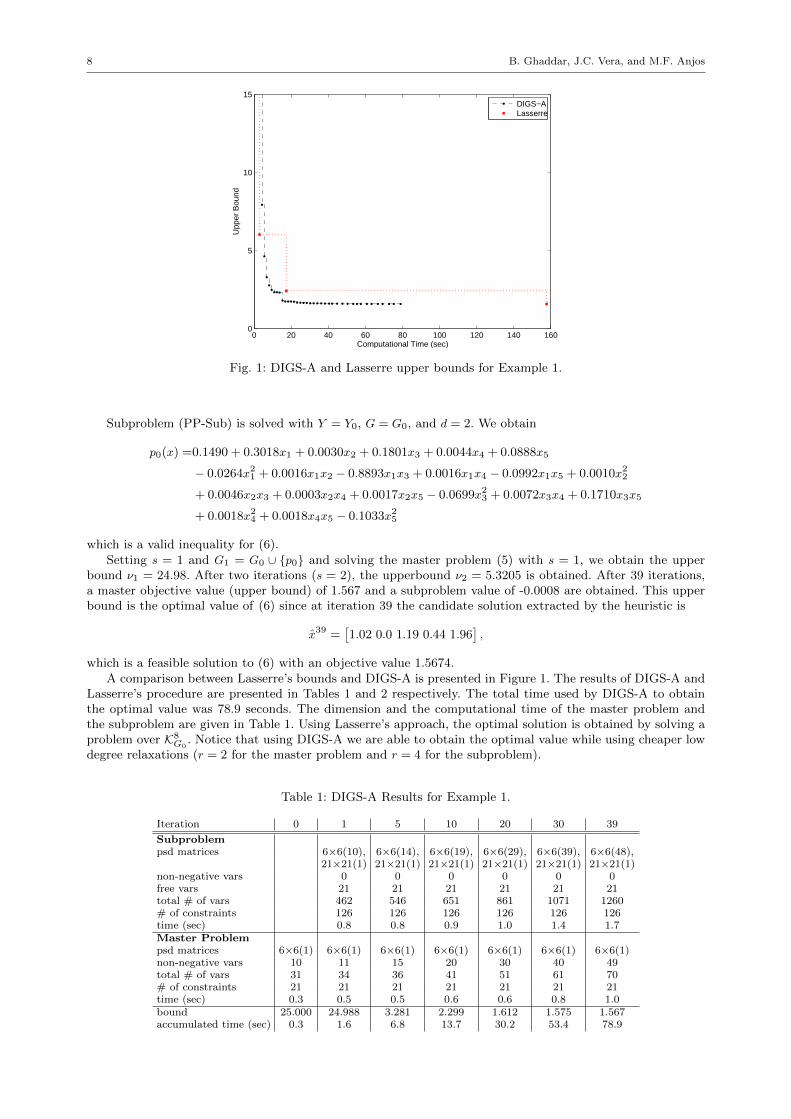
Fig. 1: DIGS-A and Lasserre upper bounds for Example 1.

Subproblem (PP-Sub) is solved with Y = Y0, G = G0, and d = 2. We obtain

p0(x) =0.1490 + 0.3018x1 + 0.0030x2 + 0.1801x3 + 0.0044x4 + 0.0888x5

− 0.0264x21 + 0.0016x1x2 − 0.8893x1x3 + 0.0016x1x4 − 0.0992x1x5 + 0.0010x22

+ 0.0046x2x3 + 0.0003x2x4 + 0.0017x2x5 − 0.0699x23 + 0.0072x3x4 + 0.1710x3x5

+ 0.0018x24 + 0.0018x4x5 − 0.1033x25

which is a valid inequality for (6).Setting s = 1 and G1 = G0 ∪ {p0} and solving the master problem (5) with s = 1, we obtain the upper

bound ν1 = 24.98. After two iterations (s = 2), the upperbound ν2 = 5.3205 is obtained. After 39 iterations,a master objective value (upper bound) of 1.567 and a subproblem value of -0.0008 are obtained. This upperbound is the optimal value of (6) since at iteration 39 the candidate solution extracted by the heuristic is

x39 =[1.02 0.0 1.19 0.44 1.96

],

which is a feasible solution to (6) with an objective value 1.5674.A comparison between Lasserre’s bounds and DIGS-A is presented in Figure 1. The results of DIGS-A and

Lasserre’s procedure are presented in Tables 1 and 2 respectively. The total time used by DIGS-A to obtainthe optimal value was 78.9 seconds. The dimension and the computational time of the master problem andthe subproblem are given in Table 1. Using Lasserre’s approach, the optimal solution is obtained by solving aproblem over K8

G0. Notice that using DIGS-A we are able to obtain the optimal value while using cheaper low

degree relaxations (r = 2 for the master problem and r = 4 for the subproblem).

Table 1: DIGS-A Results for Example 1.

Iteration 0 1 5 10 20 30 39

Subproblempsd matrices 6×6(10), 6×6(14), 6×6(19), 6×6(29), 6×6(39), 6×6(48),

21×21(1) 21×21(1) 21×21(1) 21×21(1) 21×21(1) 21×21(1)non-negative vars 0 0 0 0 0 0free vars 21 21 21 21 21 21total # of vars 462 546 651 861 1071 1260# of constraints 126 126 126 126 126 126time (sec) 0.8 0.8 0.9 1.0 1.4 1.7Master Problempsd matrices 6×6(1) 6×6(1) 6×6(1) 6×6(1) 6×6(1) 6×6(1) 6×6(1)non-negative vars 10 11 15 20 30 40 49total # of vars 31 34 36 41 51 61 70# of constraints 21 21 21 21 21 21 21time (sec) 0.3 0.5 0.5 0.6 0.6 0.8 1.0bound 25.000 24.988 3.281 2.299 1.612 1.575 1.567accumulated time (sec) 0.3 1.6 6.8 13.7 30.2 53.4 78.9


Table 2: Lasserre’s Hierarchy for Example 1.

r 2 4 6 8

psd matrices 6×6(1) 6×6(10), 21×21(10), 56×56(10),21×21(1) 56×56(1) 126×126(1)

non-negative vars 10 0 0 0total # of vars 31 441 3906 23961# of constraints 21 126 462 1287bound 25.000 6.006 2.399 1.567time (sec) 0.3 2.9 17.3 157.7

2.2 DIGS-A+: DIGS for polynomial programs with non-negative variables

We now consider the case in which the feasible set is contained in the non-negative orthant. Let R+d [x] denote

the cone of polynomials in n variables with non-negative coefficients of degree at most d. Lasserre’s relaxationscan be applied replacing the cone Σd of SOS by the cone Σd + R+

d [x] of polynomials that can be representedas a sum of squares plus a polynomial with non-negative coefficients.

For S = {x : gi(x) ≥ 0, i = 1, . . . ,m} ⊆ Rn+, consider the following approximation of P(S):

CPrG =m∑i=0

gi(x)(Σr−deg(gi) + R+r−deg(gi)

[x]). (7)

The corresponding optimization problem, (CP-Ms), over S can be written as:

νs = sup λ

s.t. f(x)− λ =m∑i=0

(σi(x) + γi(x))gi(x) +s∑i=1

(ηi(x) + εi(x))pi(x) (8)

σi(x) ∈ Σr0−deg(gi), γi(x) ∈ R+r−deg(gi)

[x] i = 0, . . . ,m

ηi(x) ∈ Σr0−deg(pi), εi(x) ∈ R+r−deg(pi)

[x] i = 1, . . . , s.

If (PP-P) has m inequality constraints at iteration s of Algorithm 1, the size of (8) is:

– m+ 1 psd matrices, each of size (n+r0−deg(gi)r0−deg(gi)

) for i ∈ {0, 1, . . . ,m};

– s psd matrices, each of size (n+r0−deg(pi)r0−deg(pi)

) for i ∈ {1, . . . , s} ;

–∑mi=0 (n+r0−deg(gi)

r0−deg(gi)) +

∑si=1 (n+r0−deg(pi)

r0−deg(pi)) non-negative variables;

– (n+r0r0) linear constraints.

The subproblem is of the form

(CP-Sub) minp〈p, Y 〉 (9)

s.t. (1 +n∑i=1

xi)p(x) ∈ CPr0+1G ∩Rr0 [x]

‖ p ‖ ≤ 1.

We call the resulting scheme DIGS-A+ and present it as Algorithm 3.

DIGS-A+ is computationally more efficient than DIGS-A. Even though the master problem for DIGS-A+

is larger due to the non-negative variables, at each iteration subproblem (9) has n+r0+1r0+1 times the number

of variables and n+r0+1r0+1 times the number of constraints of the master problem. This is much smaller than

subproblem (4) in DIGS-A.

2.2.1 Examples

We present four examples comparing the bounds obtained using DIGS-A, DIGS-A+ and Lasserre’s hierarchy.For DIGS-A and DIGS-A+ we stop when the objective value of the subproblem is greater than −ε = −10−3.All the algorithms are given a time limit of 5 hours (18000 seconds).


Algorithm 3 DIGS-A+:DIGS for polynomial programs with non-negatives variables

Require: G description of S ⊆ R+, r0 ≥ d, ε > 0s← 0, G0 ← G.loop

Let

(CP-Ms) νs = supλ

λ

s.t. f(x)− λ ∈ CPr0Gs.

Ys ← dual optimal solution to (CP-Ms).Let ps(x) ∈ Rr0 [x] be optimal solution of

αs = minp〈p, Ys〉

s.t. (1 +n∑i=1

xi)p(x) ∈ CPr0+1Gs

∩Rr0 [x]

‖ p ‖ ≤ 1.


elseSTOP

end ifend loop

Example 2

Consider the following polynomial program of degree 2:

maxx∈R

x1 + x2 − x3 + 2x4 + x5 − x6 − x7 + x8 − x9 + 2x10

s.t. (x3 − 2)2 − (x5 − 1)2 − 2x6 + x28 − (x9 − 2)2 ≥ −4

− x22 + x3x10 − x24 − x25 + x6x7 ≥ 1

x1x8 − x2x3 + x4x7 − x5x10 ≥ 2

10∑i=1

xi ≤ 5

xi ≥ 0 ∀i ∈ {1, . . . , 10}.

Tables 3a, 3b, and 3c present bounds and computational time for Lasserre’s method, DIGS-A (r0 = 2),and DIGS-A+ (r0 = 2) respectively. Figure 2 illustrates the bound improvements.

Table 3: Bounds for Example 2.

(a) Lasserre’s method

r 2 4 6

bound 10.000 7.756 5.183*T(sec) 0.2 35.8 4012.7

(b) DIGS-A

Iter. 0 1 5 9

bound 10.000 9.992 5.276 5.183*T(sec) 0.2 15.9 66.2 114.9

(c) DIGS-A+

Iter. 0 1 5 9

bound 7.760 5.749 5.192 5.183*T(sec) 0.3 2.4 9.4 16.3

Values with ∗ indicate termination reporting optimality.

100

101

102

103

104

5

5.5

6

6.5

7

7.5

8

8.5

9

9.5

10

10.5


Upp

er B

ound

DIGS−ADIGS−A+Lasserre

Fig. 2: Bounds comparison for Example 2.

All three approaches find the optimal value 5.183. For r = 6 Lasserre’s method stops with the momentmatrix optimality condition satisfied, obtaining the optimal solution in just over one hour.


Using DIGS-A and DIGS-A+ with r0 = 2, degree-two relaxations are used to obtain the optimal value inmuch less computational time. Both require the same number of iterations, but DIGS-A+ is seven times fasterthan DIGS-A and 250 times faster than Lasserre’s r = 6 relaxation. For DIGS-A, at iteration 9, the heuristicfinds the solution x1 = x8 = 1.4143, x3 = 0.6628, x10 = 1.5088, and x2 = x4 = x5 = x6 = x7 = x9 = 0 whichis optimal (tolerance of 10−3). For DIGS-A+, also at iteration 9, the heuristic finds the solution x1 = 1.4137,x3 = 0.6627, x8 = 1.4146, x10 = 1.5089, and x2 = x4 = x5 = x6 = x7 = x9 = 0 which is also optimal (toleranceof 10−3).

Example 3


maxx∈R

− 2x1 + x2 − x3 + 2x4 + x5 − x6 − x7 + x8 − x9 + 2x10

s.t. (x1 − 2)2 − x22 − (x7 − 2)2 − (x5 − 1)2 + (x6 − 2)2 + x210 ≥ 0

x24 − x21 − (x3 − 1)2 − (x8 − 2)2 + (x9 − 2)2 + (x10 − 2)2 ≥ 0

x3x8 − x4x5 + x21 + x6x9 + x1x7 ≥ 1

10∑i=1

xi ≤ 10

xi ≥ 0 ∀i ∈ {1, . . . , 10}.

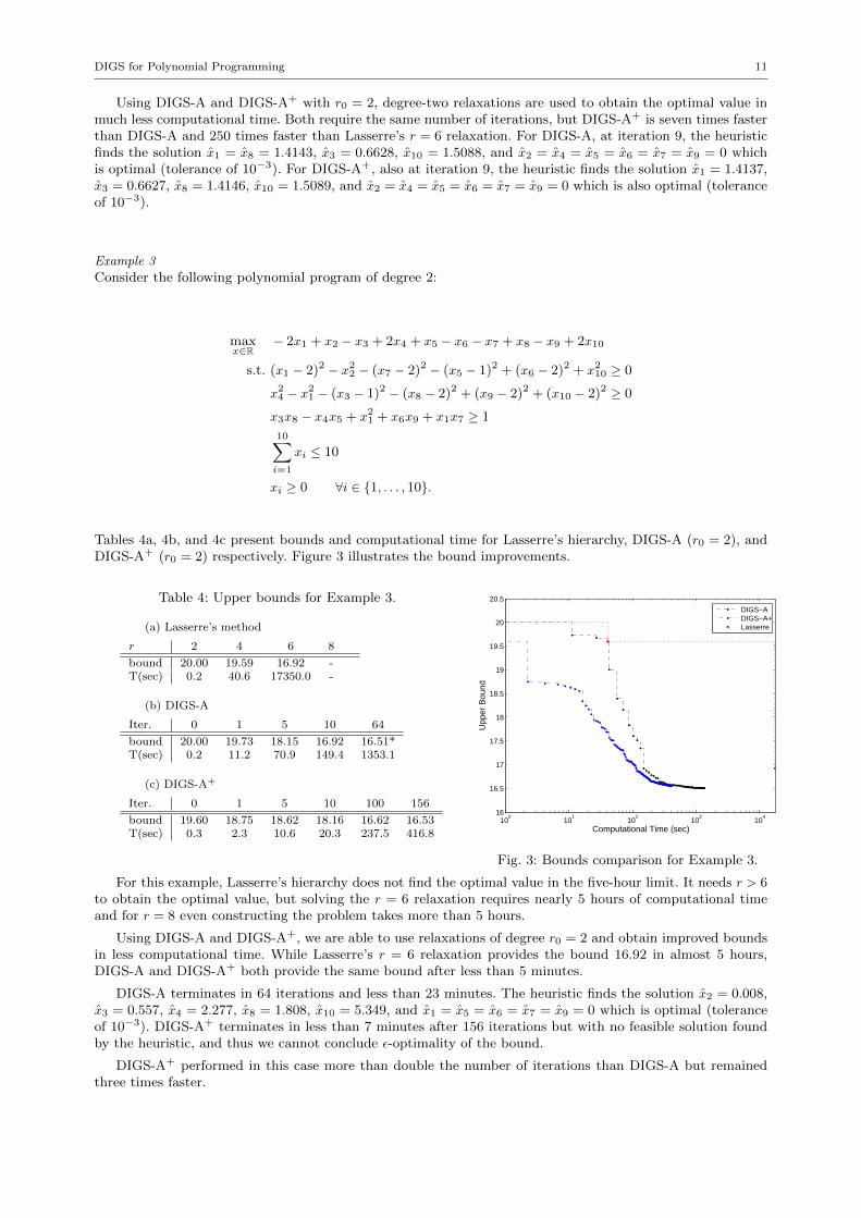
Tables 4a, 4b, and 4c present bounds and computational time for Lasserre’s hierarchy, DIGS-A (r0 = 2), andDIGS-A+ (r0 = 2) respectively. Figure 3 illustrates the bound improvements.

Table 4: Upper bounds for Example 3.


r 2 4 6 8

bound 20.00 19.59 16.92 -T(sec) 0.2 40.6 17350.0 -

(b) DIGS-A

Iter. 0 1 5 10 64

bound 20.00 19.73 18.15 16.92 16.51*T(sec) 0.2 11.2 70.9 149.4 1353.1

(c) DIGS-A+

Iter. 0 1 5 10 100 156

bound 19.60 18.75 18.62 18.16 16.62 16.53T(sec) 0.3 2.3 10.6 20.3 237.5 416.8

100

101

102

103

104

16

16.5

17

17.5

18

18.5

19

19.5

20

20.5


Upp

er B

ound


Fig. 3: Bounds comparison for Example 3.

For this example, Lasserre’s hierarchy does not find the optimal value in the five-hour limit. It needs r > 6to obtain the optimal value, but solving the r = 6 relaxation requires nearly 5 hours of computational timeand for r = 8 even constructing the problem takes more than 5 hours.

Using DIGS-A and DIGS-A+, we are able to use relaxations of degree r0 = 2 and obtain improved boundsin less computational time. While Lasserre’s r = 6 relaxation provides the bound 16.92 in almost 5 hours,DIGS-A and DIGS-A+ both provide the same bound after less than 5 minutes.

DIGS-A terminates in 64 iterations and less than 23 minutes. The heuristic finds the solution x2 = 0.008,x3 = 0.557, x4 = 2.277, x8 = 1.808, x10 = 5.349, and x1 = x5 = x6 = x7 = x9 = 0 which is optimal (toleranceof 10−3). DIGS-A+ terminates in less than 7 minutes after 156 iterations but with no feasible solution foundby the heuristic, and thus we cannot conclude ε-optimality of the bound.

DIGS-A+ performed in this case more than double the number of iterations than DIGS-A but remainedthree times faster.


Example 4


maxx∈R

− x1 + x2 − x3 + x4 + x5 − x6 − x7 + x8 − x9 + x10 − x11 + x12 − x13 + x14 − x15

s.t. (x1 − 2)2 − x22 + (x3 − 2)2 − (x4 − 1)2 − (x5 − 1)2 + (x6 − 1)2 − (x7 − 2)2 − x28− (x9 − 2)2 − (x10 − 1)2 + x211 − x212 + (x13 − 2)2 + x214 − (x15 − 1)2 ≥ 0

− x1x7 − x4x5 − x213 + x6x9 + x10x12 ≥ 3

x2x3 − x8x11 − x214 + x5x15 ≥ 3

15∑i=1

xi ≤ 10

xi ≥ 0 ∀i ∈ {1, . . . , 15}.

Table 5a presents Lasserre’s Hierarchy results. As in the previous examples, quadratic inequalities (r0 = 2)are added using DIGS-A and DIGS-A+ to improve the bound. Tables 5b and 5c present the bounds andcomputational time for DIGS-A and DIGS-A+ respectively.

Table 5: Upper bounds for Example 4.


r 2 4 6

bound 10.00 8.0593 -T(sec) 0.3 2754.3 -

(b) DIGS-A

Iter. 0 1 5 10 18

bound 10.00 10.00 7.93 7.58 7.43*T(sec) 0.3 717.8 3128.0 5720.1 10236.1

(c) DIGS-A+

Iter. 0 1 5 7

bound 8.07 7.67 7.44 7.43*T(sec) 0.6 6.7 33.4 43.9

100

101

102

103

104

7

7.5

8

8.5

9

9.5

10

10.5


Upp

er B

ound


Fig. 4: Bounds comparison for Example 4.This example illustrates how the dimension affects the three methods. Lasserre’s relaxations could not

be solved for r > 4 due to memory and time limitations. Both DIGS-A and DIGS-A+ obtain better boundsthan Lasserre’s r = 4 relaxation, and DIGS-A+ outperforms DIGS-A (see Figure 4). Indeed DIGS-A+ isthree orders of magnitude faster than DIGS-A and nevertheless both DIGS-A and DIGS-A+ terminate (after7 and 18 iterations respectively) with the optimal objective value of 7.43 and ε-optimal heuristic solutionx1 = x3 = x6 = x7 = x9 = x13 = 0.0000, x2 = 0.5881, x4 = 0.3344, x5 = 2.6244, x8 = 0.5673, x10 = 2.3443,x11 = 0.0008, x12 = 1.6538, x14 = 0.6047, and x15 = 1.2822.

Example 5

This is an example where DIGS-A+ fails to converge to the optimal solution of the polynomial program. ThePP is a formulation of the maximum stable set number for the icosahedron graph.

Given an undirected graph G = (V,E), a stable set of G is a set of vertices U ⊆ V such that there is no edgeconnecting any two vertices in U . The stable set number problem is to find α(G) the maximum k for whichthe graph has a stable set of cardinality k. Letting n = |V |, and identifying V with {1, . . . , n}, the maximumstable set problem can be formulated as follows:

(SS-POP) α(G) = maxx

(n∑i=1

xi

)2

(10)

s.t. xixj = 0 ∀(i, j) ∈ En∑i=1

x2i = 1

x ≥ 0.

Notice that Lasserre’s relaxation of (SS-POP) for r = 2 is equivalent to the Lovasz theta relaxation. Thus,DIGS-A and DIGS-A+ can be interpreted here as adding quadratic valid inequalities to strengthen the Lovasztheta relaxation.


We consider the case in which G is the icosahedron graph on n = 12 vertices (see Figure 5). ApplyingDIGS-A+ results in an objective function of 3.236 at the initial iteration, and the algorithm immediately stopsbecause the subproblem objective function value is of order −10−8. However, using Lasserre’s hierarchy forr = 4 gives the optimal bound 3.000. DIGS-A terminates in 16 iterations with the bound 3.002.

−3 −2 −1 0 1 2 3−2

−1.5

−1

−0.5

0

0.5

1

1.5

2

2.5

3

Fig. 5: Icosahedron graph for Example 5.

Table 6: Bounds for Example 5.


r 2 4 6

bound 3.708 3.000 -T(sec) 0.1 94.8 -

(b) DIGS-A

Iter. 0 1 5 10 16

bound 3.708 3.164 3.002 3.002 3.002T(sec) 0.1 31.9 209.2 547.9 1057.5

(c) DIGS-A+

Iter. 0 1

bound 3.2361 3.2361T(sec) 0.1 2.0

3 The Special Case of Binary Polynomial Programs

This section focus on the special case of polynomial programs with binary variables. We specialize Algorithm1 to this class of problems and propose a specialized DIGS called DIGS-B. The main improvement in DIGS-Bis the use of a computationally cheaper subproblem for the binary case. The subproblem is obtained using theapproach proposed in [28] and [37]. Furthermore, we show that if the initial set of constraints G is rich enough,the stopping criterion is optimal, that is, DIGS-B only stops when optimality is reached. Theorems 1 and 2show that DIGS-B terminates only at optimality when starting from the exact representation of the domain setexcluding the binary constraints. Such a representation is not tractable in general, but these results hint thatif our approximation QG of Pd(S ∩ {−1, 1}n) captures enough of Pd(S), then the optimality criterium couldbe applied. Recall that we use a heuristic approach (see Section 2.1.1) to check optimality. The advantage ofthis heuristic approach is that when successful it also generates an optimal solution. Theorem 3 shows that aLP-variation of DIGS-B always stops after a finite number of iterations.

Several techniques have been developed to construct hierarchies of linear and semidefinite relaxations tosolve binary linear programs; in particular, by Balas, Ceria, and Cornuejols [3], Sherali and Adams [32], andLovasz and Schrijver [19]. The method presented in this section can be seen as a generalization of the lift-and-project methods based on these hierarchies. For the pure binary case, Lasserre [14] presents necessary andsufficient conditions under which his method converges to the optimal objective value of the 0-1 polynomialprogram after a finite sequence of liftings. A comparison of these different schemes and bounds on the numberof steps required for convergence is given by Laurent [17].

3.1 DIGS-B: DIGS for polynomial programs with binary variables

We assume that the feasible set of (PP-P) has the form S = D∩{−1, 1}n where D = {x : gi(x) ≥ 0, i = 1, . . . ,m}.We further assume without loss of generality that D ⊆ [−1, 1]n; this can be ensured for example by adding theinequalities −1 ≤ xi ≤ 1 to the definition of D. Problem (PP-D) becomes

ρ = supλλ (11)

s.t. f(x)− λ ∈ Pd(D ∩ {−1, 1}n).

Proceeding similarly as in Section 2, we let G = {g0(x), g1(x), . . . , gm(x)} where g0(x) = 1. Define QrG asthe following approximation to Pd(S):

QrG =

|G|∑i=0

gi(x)Σr−deg(gi) +n∑i=1

(1− x2i )Rr−2[x]


Fix r0 ≥ d and define the polynomial programming master problem

ϕr0G = supλλ (12)

s.t. f(x)− λ ∈ Qr0G ,

which can be written as

ϕr0G = supλ,σi(x),δi(x)

λ

s.t. f(x)− λ =m∑i=0

σi(x)gi(x) +n∑i=1

δi(x)(1− x2i ).

σi(x) ∈ Σr0−deg(gi), i = 0, 1, . . . ,m

δi(x) ∈ Rr0−2[x], i = 1, . . . , n.

Let Hj = {x ∈ Rn : xj ∈ {−1, 1}} and H = {−1, 1}n. Notice that H =⋂j∈{1,...,n}Hj . Instead of solving

the polynomial generating subproblem over Qr0+2G as defined in Section 2.1, we use Proposition 2 to obtain a

computationally-cheaper polynomial generating subproblem.

Proposition 2 [28] For any degree d and compact set D,

Pd(D ∩Hj) =(

(1 + xj)Pd(D) + (1− xj)Pd(D) + (1− x2j )Rd−1[x])∩Rd[x].

From Proposition 2, defining for any Q ⊆ Rr0 [x],

Cr0j (Q) :=(1 + xj)

2Q+

(1− xj)2

Q+ (1− x2j )Rr0−1[x],

we have Cr0j (Pd(D))∩Rd[x] = Pd(D∩Hj) for any r0 ≥ d and any compact set D. Another important property

of the operator Cr0j is that if Q ( Pd(S) then (Cr0j (Q)\Q)∩Rd[x] 6= ∅ for some j (see Lemma 3). This property

is critical to obtain a more efficient DIGS for the binary case: when looking for improving inequalities, Cr0j (Qr0G )

can be used instead of Qr0+2G in the definition of Subproblem (PP-Sub), resulting in a much smaller subproblem.

Let Y be the optimal dual variable for (12), then the j-th polynomial generating subproblem for the binarycase is defined as

minp〈p, Y 〉 (13)

s.t. p ∈ Cr0j (Qr0G ) ∩Rr0 [x]

‖ p ‖≤ 1.

Replacing the master problem and subproblem in Algorithm 2 by (12) and (13) respectively, we obtainDIGS-B (Algorithm 4).

DIGS-B terminates when the subproblem (13) has objective value equal to zero for all indexes j. In practice,the algorithm stops when the value of every subproblem is sufficiently close to zero.

For the binary case, DIGS-B is a priori computationally more efficient than DIGS-A. The master problemsare of the same size but solving the subproblem (13) is of the same order as solving the master problem (12),since at each iteration, (13) has twice the number of variables and n+r0+1

r0+1 times the number of constraints of

the master problem. This is significantly smaller than subproblem (4) for the general case which has O(n2/r20)times the number of variables and O(n2/r20) times the number of constraints compared to the master problem.

3.2 Optimality and Finiteness of DIGS-B

In general we do not expect our algorithms to stop, or even if they do, we do not expect them to alwaysprovide the optimal value (see example 5). In this section, we prove (see Theorems 1 and 2) that under someassumptions DIGS-B certifies optimality for binary polynomial programs. Optimality is certified in the sensethat if DIGS-B stops, i.e., if all sub-problems have optimal value zero, then the bound provided by DIGS-B isequal to the optimal value of (11). We also prove (Theorem 3) finite termination for DIGS-B∗ (see Algorithm5), a variation of DIGS-B.


Algorithm 4 DIGS-B: DIGS for binary polynomial problems

Require: G description of S, r0 ≥ d, ε > 0s← 0, G0 ← G.loop

Let

(BP-Ms) νs = supλ

λ

s.t. f(x)− λ ∈ Qr0Gs.

Ys ← dual optimal solution to (BP-Ms).LET ps(x) ∈ Rr0 [x] be an optimal solution of

αs = minj=1,...,n

minp〈p, Ys〉

s.t. p ∈ Cj(Qr0Gs) ∩Rr0 [x]

‖ p ‖≤ 1,


elseSTOP

end ifend loop

First we discuss the properties of the operator Cdj that will be key for our results.

Lemma 3 Let D ⊂ [−1, 1]n and let Q ⊆ Pd(D ∩H).

1. For every j and r0 ≥ d, Q ⊆ Cr0j (Q) ∩Rd[x] ⊆ Pd(D ∩H),

2. If Pd(D) ⊆ Q then Pd(D ∩Hj) ⊆ Cr0j (Q) ∩Rd[x],

3. Moreover, if Pd(D) ⊆ Q ( Pd(D ∩H) then for some j, Q ( Cr0j (Q) ∩Rd[x].

Proof

1. From the definition of Cr0j , Q ⊆ (1−xj)2 Q+

(1+xj)2 Q ⊆ Cr0j (Q). On the other hand if Q ⊆ Pd(D ∩H) then

(1−xj)2 Q, (1+xj)

2 Q ⊆ Pd+1(D ∩H) and thus Cr0j (Q) ⊆ Pr0+1(D ∩H).2. Follows from Proposition 2.3. For the sake of contradiction, assume Q = Cr0j (Q)∩Rd[x] for all j. Applying part 2 for all i = 1, . . . , n we have

Pd(D∩⋂j≤iHj) ⊆ C

r0i (Pd(D∩

⋂j≤i−1Hj))∩Rd[x] and by induction it follows that Pd(D∩

⋂j≤iHj) = Q

for all i = 1, . . . , n. In particular Pd(D ∩H) ⊆ Q.ut

Recall from (3) that the optimal dual solution Y ∈ {X ∈ (QdG)∗ : 〈1, X〉 = 1}. When D is compact, theset Pd(D)∗ can be characterized in terms of truncated moment matrices of atomic measures, using classicaltheorems from [?] and [?] (see [?, Thms 5.9 and 5.13]). Using the compactness of D implies that Pd(D)∗

is pointed, {Pd(D)∗ : 〈1, X〉 = 1} could be then characterized in terms of truncated moment matrices ofatomic probability measures, which are themselves convex combinations of truncated moment matrices ofDirac measures. Truncated moment matrices of Dirac measures are in correspondence with Md(u), the vector

of monomials of u up to degree d for some u. All this is subsumed in Proposition 3, where {Pd(D)∗ : 〈1, X〉 = 1} ischaracterized as the convex hull ofMd(D) = {Md(u) : u ∈ D}, for compact D. A more elemental, self-containedproof is also given.

Proposition 3 Let D ⊆ Rn be a compact set, then

{X ∈ Pd(D)∗ : 〈1, X〉 = 1} = conv(Md(D)).

Proof By definition,

Md(D)∗ = {p : 〈p,X〉 ≥ 0 ∀X ∈Md(D)}= {p : 〈p,Md(s)〉 ≥ 0 ∀s ∈ D}= {p : p(s) ≥ 0 ∀s ∈ D}= Pd(D).

Therefore, Pd(D)∗ =Md(D)∗∗ = closure(cone(conv(Md(D)))). Since D is compact, Md(D) is compact. Also,for all x ∈ D, 〈1,Md(x)〉 = 1 and thus

{X ∈ Pd(D)∗ : 〈1, X〉 = 1} = {X ∈Md(D)∗∗ : 〈1, X〉 = 1} = conv(Md(D)).

ut


The set convM2({−1, 1}n) is closely related to conv{xxT : x ∈ {−1, 1}n}, the Boolean Quadratic Polytope [8,9].More generally conv{Md(u) : u ∈ D} is a polytope for any finite D. We will use this fact later in the proof ofTheorem 3.

Lemma 4 Let d ≥ 1 and let D be a finite set. Then convMd(D) is a polytope, and Pd(D) is a polyhedral cone.

3.2.1 Optimality

In this section we prove optimality for DIGS-B under certain conditions. More precisely we show that if thestarting set G is such that the approximation Qr0G contains Pd(D), DIGS-B only stops if the bound given bythe master problem is optimal. If Qr0G ⊇ Pd(D) then subproblem (13) is equivalent to optimizing over a setcontaining Pd(D ∩ Hj) (by Lemma 3, part 2). Intuitively, if the subproblem has a value of 0, it is becauserestricting xj to be binary does not change the objective value. Thus if the value of all subproblems is zero,then the algorithm has converged to the optimal value. This intuition is formally expressed in Theorems 1 and2.

Theorem 1 Let d ≥ 2. Suppose that D ⊆ [−1, 1]n is a compact set, and that r0 ≥ d and G := {gi(x) : i =1, . . . ,m} ⊂ R[x] are such that Pd(D) ⊆ Qr0G ∩Rd[x] ⊆ Pd(D ∩ {−1, 1}n). If the optimal value of subproblem (13)is zero for all j = 1, . . . , n, then the optimal value of the dual problem of the master (12) equals the optimal value of

the original binary polynomial program (11).

Proof Let Q = Qr0G ∩ Rd[x]. Let ρ be the optimal value of (11) and ωj be the optimal value of the j-thsubproblem (13). Further let ϕ be the optimal value and Y be an optimal solution of the dual problem of (12).Since Q ⊆ Pd(D ∩ {−1, 1}n) then ϕ≤ρ. By Proposition 3,

Y ∈ {X ∈ Q∗ : 〈1, X〉 = 1} ⊆ {X ∈ Pd(D)∗ : 〈1, X〉 = 1} = conv(Md(D)).

As D is compact, conv(Md(D)) is compact, and by Caratheodory’s Theorem, Y can be expressed in the formY =

∑i aiMd(ui) with ai > 0,

∑i ai = 1 and every ui ∈ D. It follows that for any p ∈ Rd[x] we have 〈p, Y 〉 =∑

i ai 〈p,Md(ui)〉 =∑i aip(ui). It is enough to show that ui ∈ H for all i, as then ϕ = 〈f, Y 〉 =

∑i aif(ui)≥ρ

and we are done. Assume, there exists uk /∈ H for some k. Then there is a j ≤ n such that uk /∈ Hj . Considerp(x) = 1− x2j . We have

ωj ≥ 〈p, Y 〉 as p(x) ∈ Cr0j (Qr0G )

=∑i

aip(ui)

≥ akp(uk) as for all i, ui ∈ D ⊆ [−1, 1]n

> 0, because uk /∈ Hj

which is a contradiction. ut

For d ≥ 4 the condition D ⊆ [−1, 1]n can be dropped from Theorem 1. This allows more freedom in choosingthe set D.

Theorem 2 Let d ≥ 4. Suppose that D is a compact set, and that r0 ≥ d and G := {gi(x) : i = 1, . . . ,m} ⊂ R[x]are such that Pd(D) ⊆ Qr0G ∩ Rd[x] ⊆ Pd(D ∩ {−1, 1}n). If the optimal value of subproblem (13) is zero for all

j = 1, . . . , n, then the optimal value of the dual problem of the master (12) equals the optimal value of the original

binary polynomial program (11).

Proof We follow the lines of the proof of Theorem 1. We write Y as the convex combination Y =∑i aiMd(ui),

where each ui ∈ D. Again, it is enough to show that each ui belongs to H.Consider p(x) = −x4j + 2x2j − 1 = −(x2j − 1)2 ∈ Cr0j (Qr0G ). We have,

0 ≤ 〈p, Y 〉 = −∑i

aiu4ij + 2

∑i

aiu2ij − 1. (14)

Now consider q(x) = 1− x2j ; we have ±q(x) ∈ Cr0j (Qr0G ), and thus

0 ≤ 〈±q, Y 〉 = ±∑i

aiq(ui) = ±

(1−

∑i

aiu2ij

),

and thus, ∑i

aiu2ij = 1. (15)


Plugging (15) into (14) we obtain ∑i

aiu4ij ≤ 1. (16)

Now, using the Cauchy-Schwarz inequality,

1 =

(∑i

aiu2ij

)2

≤

(∑i

aiu4ij

)(∑i

ai

)=∑i

aiu4ij (17)

Using (16), equality follows in (17), and thus for each i we have√aiu

2ij = t

√ai for some constant t. Therefore,

u2ij = t for all i and from Equation (15):∑i ait = 1, that is t = 1. ut

Using that when DIGS-B stops, all the subproblems have value 0, we obtain the following corollary toTheorems 1 and 2.

Corollary 1 Let D be a compact set. Assume d ≥ 4, or d ≥ 2 and D ⊆ [−1, 1]n. Let r0 ≥ d and G := {gi(x) : i =1, . . . ,m} ⊂ R[x] be a description of D ∩ {−1, 1}n such that Pd(D) ⊆ Qr0G . Assume DIGS-B (Algorithm 4) is run

starting with G0 = G, and it stops with all subproblems having value 0. Then, at stopping, the optimal value of the

dual problem of the master (12) equals the optimal value of the original binary polynomial program (11).

Proof Notice that as G is a description of D ∩ {−1, 1}n we have Qr0G ∩Rd[x] ⊆ Pd(D ∩ {−1, 1}n). Also Pd(D) ⊆Qr0G ∩Rd[x] by assumption. By induction, At each iteration s ≥ 0, we have Pd(D) ⊆ Qr0Gs

∩Rd[x] ⊆ Pd(D ∩{−1, 1}n). Thus if DIGS-B stops at iteration k, the assumptions of Theorem 1 or Theorem 2 hold for G = Gk.

ut

3.2.2 Finite Termination

For the next theorem we need to define a variation of DIGS-B which we refer to as DIGS-B∗. We show thatDIGS-B∗ stops after a finite number of steps. Notice that Theorems 1 and 2 also hold for this version ofDIGS-B (i.e. replacing QrG by QrG). To ensure finite termination, we use polyhedral approximations to the setPd(D ∩ {−1, 1}n). Recall that for any D the set Pd(D ∩ {−1, 1}n) is a polyhedron (Lemma 4).

Proceeding similarly as in Section 3.1, we let G = {g0(x), g1(x), . . . , gm(x)} where g0(x) = 1. Define QrG asthe following approximation to Pd(D ∩ {−1, 1}n):

QrG =

|G|∑i=0

gi[1− x, 1 + x]R+r−deg(gi)

[x] +n∑i=1

(1− x2i )Rr−2[x]

Fix r0 ≥ d and define the polynomial programming master problem

ϕr0G = supλλ

s.t. f(x)− λ ∈ Qr0G ,

which can be written as

ϕr0G = supλ,σi(x),δi(x)

λ

s.t. f(x)− λ =m∑i=0

σi(x)gi(x) +n∑i=1

δi(x)(1− x2i ).

σi(x) ∈ R+r0−deg(gi)

[x], i = 0, 1, . . . ,m

δi(x) ∈ Rr0−2[x], i = 1, . . . , n.

In each iteration of DIGS-B∗ we add to the master problem the inequality produced by the subproblemwith negative value of largest index. The main differences with the DIGS-B subproblem, besides using thepolyhedral approximation, is that we use the 1-pseudo-norm, ‖p‖1 =

∑0<‖α‖≤r0 |pα| and for the j-subproblem

we only take into account inequalities added when using subproblems of lower index. Thus we maintain aseparate list of inequalities for each index. With these changes the master and all subproblems are linearprograms.


Algorithm 5 DIGS-B∗: DIGS for binary polynomial problems

Require: G description of S, r0 ≥ d,

s← 0, Gj0 =← G for j = 1, . . . , nloop

Let

(BP-Ms) νs = supλ

λ

s.t. f(x)− λ ∈ Qr0Gns.

Ys ← dual optimal solution to (BP-Ms).

LET pjs(x) ∈ Rr0 [x] be an optimal (extreme) solution of

αjs = minp〈p, Ys〉

s.t. p ∈ Cr0j (Qr0G

js

) ∩Rr0 [x]

‖ p ‖1≤ 1,

if αjs ≥ 0 for all j = 1, . . . , n thenSTOP

elseLET j∗s = max{j : αjs < 0}Gis+1 ← Gis ∪ {p

j∗ss (x)} for i = j∗s , . . . , n

s← s+ 1end if

end loop

Theorem 3 Algorithm 5 terminates in finitely many iterations.

Proof For sake of contradiction, assume Algorithm 5 does not stop for some d > 0 some finite G ⊂ Pd(S) andsome r0 ≥ d. Consider the infinite sequence 〈j∗s 〉s=1,2,3,... generated by the algorithm. As each j∗s ∈ {1, . . . , n},the set Ui = {s : j∗s = i} is infinite for some 1 ≤ i ≤ n. Let i∗ be the minimum such i. For each s ∈ Ui∗ we

have that pj∗ss = pi

∗s is a extreme point of Ws = {p ∈ Cr0i∗ (Qr0

Gi∗s

) ∩Rr0 [x] : ‖p‖1 = 1}. As each Ws is a polytope,

it has finitely many extreme points. Algorithm 5 does not generate repeated inequalities as every inequalitygenerated has value 0 for all subproblems in future iterations. Thus the sequence 〈Ws〉s∈Ui∗ has to changeinfinitely many times.

Now if s1 < s2 are such that j∗s1 = j∗s2 = i∗ and j∗s > i∗ for all s1 < s < s2, then Gi∗s1 = Gi

∗

s1+1 = · · · = Gi∗

s2−1

and Gi∗s2 = Gi

∗s1 ∪ {p} where p = pi

∗s2 is a extreme point of Ws2−1 = Ws1 . We claim that Ws2 = Ws1 . To show

this write

p(x) =1− xj∗

2p−(x) +

1 + xj∗

2p+(x) + (1− x2j )r(x), (18)

where p−, p+ ∈ Qr0Gi∗

s1

and r ∈ Rr0−1[x]. Notice that

1− xj∗2

p(x) =1− xj∗

2p−(x) +

1− x2j4

(2(1− xj∗)r(x) + p+(x)− p−(x)). (19)

From (18), d = deg p(x) ≥ deg(xj∗(p−(x)−p+(x)+2xjr(x))) and thus deg(p−(x)−p+(x)+2xjr(x)) ≤ d−1. Using

(19) we get1−xj∗

2 p(x) ∈ Cr0i∗ (Qr0Gi∗

s1

). Similarly,1+xj∗

2 p(x) ∈ Cr0i∗ (Qr0Gi∗

s1

) and thus Cr0i∗ (Qr0Gi∗

s2

) = Cr0i∗ (Qr0Gi∗

s1∪{p}) =

Cr0i∗ (Qr0Gi∗

s1

) and the claim follows.

We have that the sequence 〈Ws〉s∈Ui∗ has to change infinitely many times, but every time it changes thereis an s between two consecutive elements of Ui∗ such that j∗s < i∗. Therefore {s : j∗s < i∗} is infinite, but thiscontradicts the selection of i∗. ut

3.3 Comparison with Lift-And-Project Methods

For the case of binary linear programming, i.e. when d = 1, Algorithm 5 is equivalent to the Balas-Ceria-Cornuejols (BCC) lift-and-project method [3].

Theorem 4 Suppose D is polyhedral and f(x) is linear in (11). With r0 = 1, Algorithm 5 is equivalent to (the dual

of) BCC lift-and-project.


Proof The Theorem follows from the fact that the projection of the (linearized) BCC lifting, denoted Pj(x) in[3], is the dual of {p(x) ∈ Rd[x] : p(x) ∈ C1j (Q)}, the set of valid inequalities of the convex hull of D ∩Hj .

This fact follows by Farkas’ Lemma: if G = {aTi x ≥ bi, i = 0, 1, . . . ,m} with a0 = 0 and b0 = 1, thenQ1G :=

∑mi=1(aTi x− bi)Σ0 = P1(D). ut

We illustrate the dual relation between BCC and our approach by considering the LP relaxation of thebinary linear programming problem

min cT x

s.t. Ax ≥ b,x ∈ {−1, 1}n.

For any given j, applying BCC with the variable xj yields the lifting step

min cT x

s.t. (1 + xj)(Ax− b) ≥ 0

(1− xj)(Ax− b) ≥ 0,

where the constraints include the box constraints −1 ≤ xi ≤ 1 for all i.Next we linearize and project by substituting the product of xjxk by a new variable xjk and using the

substitution x2j = 1:

(PL) min∑i

cix0i

s.t.∑i

aikx0i +∑i

aikxij − bkx0j ≥ bk ∀k (20)∑i

aikx0i −∑i

aikxij + bkx0j ≥ bk ∀k (21)

xjj = 1. (22)

On the other hand, the problem

max λ

s.t.∑i

cixi − λ ∈ C1j (Q)

is equivalent to

maxλ

s.t.∑i

cixi − λ = (1 + xj)

[∑k

µk(aTk x− bk)

]+ (1− xj)

[∑k

νk(aTk x− bk)

]+ r(1− x2j ).

Equating the coefficients of the monomials of the left side to the ones on the right side, we obtain

maxλ

s.t. λ =∑k

µkbk +∑k

νkbk − r

cj = −∑k

bkµk +∑k

bkνk +∑k

akjµk +∑k

akjνk

ci =∑k

akjµk +∑k

akjνk

0 = −∑k

akjµk −∑k

akjνk − r

0 = −∑k

akjµk −∑k

akjνk.

Substituting λ by∑k µkbk +

∑k νkbk − r in the objective, we obtain the dual problem of (PL) where µk, νk,

and r are the dual variables of constraints (20)-(22) respectively.Theorem 4 shows that DIGS-B∗ is a generalization of BCC from degree 1 to higher degrees. This gener-

alization suggests not only solving binary PPs of degree higher than one, but also the possibility for solving


degree-one binary PPs as problems of higher degrees. In other words, when solving a binary linear programusing DIGS-B∗, setting r0 = 1 will generate the same linear inequalities as those generated by BCC. However,if we set r0 to a higher value, then we can generate valid polynomial inequalities of higher degree. It is not cleara priory which one of the two methods is more efficient. While r0 = 1 reduces to using linear programming,making each iteration much cheaper, larger values of r0 might produce stronger valid inequalities, and possiblyfewer iterations.

As an illustration, the next example compares DIGS-B with r0 = 2 to BCC (DIGS-B with r0 = 1) on themaximum stable set problem on instances taken from [27].

Example 6

The stable set number (see Example 5) can be formulated as a binary linear program as follows:

(SS-LP) α(G) = maxn∑i=1

xi

s.t. xi + xj ≤ 1 ∀(i, j) ∈ Ex ∈ {0, 1}n.

The maximum stable set problem can also be formulated as follows:

(SS-D2) α(G) = maxn∑i=1

xi

s.t. xixj = 0 ∀(i, j) ∈ Ex ∈ {0, 1}n.

We compare different versions of DIGS-B. For each instance we impose a 300-seconds time limit for eachprocedure. The upper bound obtained from BCC (i.e., by starting with the LP-relaxation of (SS-LP) andsetting r0 = 1, in which case master and subproblem are LP’s) is compared to three different variations ofDIGS-B, based on the (SS-D2) formulation. Linear refers to generating linear inequalities that are added to themaster problem by using a non-negative multiplier. SOC refers to generating linear inequalities that are addedto the master problem by using a polynomial multiplier that is in P1(B) [12]. Quadratic refers to generatingquadratic inequalities similar to the previous examples described. The results are reported in Table 7.

Table 7: Computational results for the stable set problem with a time limit of 300 seconds.

DIGS-BOptimal (SS-LP) Balas et al. (SS-D2) Linear SOC Quadratic

n value UB UB Iter. UB UB Iter. UB Iter. UB Iter.

8 3 4.00 3.00 197 3.44 3.00 186 3.00 126 3.02 4911 4 5.50 4.00 160 4.63 4.00 139 4.00 130 4.05 10914 5 7.00 5.02 135 5.82 5.02 114 5.01 91 5.14 8217 6 8.50 6.22 121 7.00 6.23 84 6.09 63 6.30 5420 7 10.00 7.46 104 8.18 7.43 68 7.25 45 7.42 3823 8 11.50 8.81 88 9.36 8.61 50 8.36 33 8.67 2226 9 13.00 10.11 77 10.54 9.84 37 9.60 25 9.96 1429 10 14.50 11.65 65 11.71 11.10 24 10.87 17 11.18 1032 11 16.00 13.03 56 12.89 12.37 18 12.20 14 12.53 635 12 17.50 14.48 49 14.07 13.49 13 13.32 10 13.66 438 13 19.00 16.05 43 15.24 14.80 8 14.74 7 14.85 441 14 20.50 17.69 39 16.42 15.88 7 15.77 6 16.26 144 15 22.00 19.10 34 17.59 17.19 6 17.09 5 17.30 147 16 23.50 20.78 29 18.77 18.39 4 18.26 4 18.59 150 17 25.00 22.18 27 19.94 19.52 4 19.42 4 19.77 1

From Table 7 it can be observe that the BCC performs the largest number of iterations for these instances. Ituses linear programming which is computationally more efficient, however this efficiency comes at the expenseof weaker improvement per iteration on the bound. On the other hand, the Quadratic approach provides thestronger average improvement per iteration but it is the method with the most expensive iterations. For allinstances the bounds obtained by using the SOC version of DIGS-B are the best within 300 seconds. Thethree options for DIGS-B present comparable bounds, even though their subproblems correspond to differentcombinations of cost and bound improvement per iteration.


3.4 Examples for the Binary Case

Unless otherwise specified, the following stopping criteria are used

– For all algorithms a time limit of 5 hours (18000 seconds) is imposed. When the algorithm does notterminate in the time limit this is expressed using a dash (-). The symbol [ besides the computational timeindicates that performing one more iteration of the algorithm will exceed the time limit.

– For DIGS-B we stop if the subproblems have a value close to 0 (≥ −10−3) or if we are able to extract afeasible solution that certifies optimality.

For the examples presented, we report the objective function value at iteration 0 and after performing a numberof iterations of DIGS-B. As a reference for comparison we also present Lasserre’s results. Values marked with∗ indicate that the approach used terminated reporting optimality.

Example 7 Degree Two BPPWe consider quadratic problems with the following formulation

max xTCx

s.t. aT x ≤ bx ∈ {−1, 1}n.

Tables 8a-8c present computational results for quadratic instances where the parameters are generatedaccording to [29]. The results are given for iterations 0, 1, 5, 10, 100, and 1000. In case the algorithm terminatesbefore the given iteration, the number of iterations reached is shown in (·). The results show that DIGS-B ismuch more efficient than Lasserre’s approach, in particular when n gets large. For n > 20, we are not able togo beyond r = 2 for Lasserre’s relaxations in the given time limit of 5 hours while using DIGS-B we are ableto improve the bounds by using this iterative scheme.

Table 8: Computational results for quadratic BPP.

(a) Lasserre’s hierarchy

r = 2 r = 4 r = 6n Optimal bound T(sec) bound T(sec) bound T(sec)

10 1653 1857.7 0.8 1707.3 28.1 1653.0* 11251.320 8510 9060.3 2.9 8639.7 17269.1 - -30 18229 19035.9 4.3 - - - -40 2679 4735.9 6.8 - - - -50 16192 21777.9 19.2 - - - -60 58451 62324.4 126.6 - - - -

(b) DIGS-A

n Optimal Iter. 0 Iter. 1 Iter. 5 Iter. 10 Iter. 100 T(sec)

10 1653 1857.7 1781.3 1735.3 1691.3 1653.0*(31) 748.9

20 8510 9060.3 8674.9 - - - 1668.4[

30 18229 19035.9 - - - - 4.3[

40 2679 4735.9 - - - - 6.8[

50 16192 21777.9 - - - - 19.2[

60 58451 62324.4 - - - - 126.6[

(c) DIGS-B

n Optimal Iter. 0 Iter. 1 Iter. 5 Iter. 10 Iter. 100 Iter. 1000 T(sec)

10 1653 1857.7 1821.9 1797.4 1782.2 1724.1 1669.8(1065) 17923.4[

20 8510 9060.3 9015.3 8925.9 8826.6 8683.2 8653.8(517) 17750.3[

30 18229 19035.9 18920.2 18807.4 18737.0 18626.2 18600.7(243) 17840.1[

40 2679 4735.9 4590.7 4248.2 4105.3 3556.7(100) - 18020.1[

50 16192 21777.9 21390.3 20162.1 19407.1 18652.7(31) - 18123.9[

60 58451 62324.4 62019.1 60906.0 60585.5 - - 17961.1[

Example 8 Degree Three BPPWe consider the general BPP problem with degree-3 objective. The problem can be formulated as follows


max∑|α|≤3

cαxα

s.t. aT x ≤ bx ∈ {−1, 1}n.

In Tables 9a-9c, we present Lasserre’s, DIGS-A, and DIGS-B results on degree three instances where cα isgenerated randomly between 0 and 10, each a is generated randomly between 1 and 50, and b is generatedrandomly between 50 and

∑ni=1 ai. The generated parameters cα, a, and b are integer.

Lasserre’s relaxation is not defined for r = 2, the smallest r we can take is r = 4. For n ≥ 25, we are notable to compute any bound using Lasserre’s relaxation within the time limit bound of 5 hours.

As we are working with a degree 3 BPP, DIGS-A is applied with a master problem of degree 3 (i.e. r0 = 3)and a subproblem of degree r0 + 1 = 4, creating inequalities of degree 2. That is, we apply Algorithm 2 withstep 3 replaced by:

minps

⟨ps, Y

s⟩s.t. ps(x) ∈ K4

Gs∩R2[x]

‖ ps ‖ ≤ 1.

The results for various iterations are reported and the total time is given in seconds. In case the algorithmterminates before the given iteration, the number of iterations reached is shown in (·).

Table 9: Computational results for degree 3 BPP.

(a) Lasserre’s hierarchy

r = 4 r = 6n Optimal bound T(sec) bound T(sec)

5 58 59.37 2.1 58.00∗ 9.610 139 148.97 35.9 139.00∗ 4866.015 1371 1524.71 1436.2 - -20 1654 1707.95 18106.6 - -25 - - - - -

(b) DIGS-A


5 58 67.16 63.59 58.37 58.00∗(8) 19.610 139 154.59 153.22 142.32 139.19 139.00∗(12) 606.3

15 1371 1582.04 1569.92 1498.60 1470.98 1429.89(23) 18037.9[

20 1654 1718.53 1716.67 - - - 16009.2[

25 - 3967.12 - - - - 5038.6[

(c) DIGS-B


5 58 67.16 58.45 58.00∗(3) 5.110 139 154.59 151.43 143.33 139.64 139.00(13)∗ 100.9

15 1371 1582.04 1550.04 1511.76 1497.37 1392.89(91) 18058.1[

20 1654 1718.53 1716.00 1709.40 1701.65 1699.70(12) 18168.6[

25 - 3967.12 3960.78 - - - 14287.3[

Table 9c presents computational results of applying Algorithm 4. We report results for iterations 0, 1, 5,and 10, 100, and 1000 and the total time in seconds. At Iteration 0, we use a relaxation of order 3 and thenapply DIGS-B to add valid degree 3 inequalities to improve the bounds of the relaxation. Comparing theresults of Table 9c with Table 9b, we see that using the specialized DIGS-B reduces the computational timesignificantly and provides better bounds.

4 Conclusion

We proposed a dynamic inequality generation scheme to generate valid polynomial inequalities for generalpolynomial programs. This scheme can be iterated to improve the SOS relaxation of a polynomial program


without incurring an exponential growth in the size of the relaxation. As a result, the proposed scheme is inprinciple scalable to large general polynomial programming problems. We also proposed specialized schemesfor polynomial programs with all variables non-negative or with all variables binary. For binary polynomialprograms, we prove that the proposed scheme converges to the global optimal solution for some problemfamilies. We presented several examples illustrating the computational behavior of the scheme and comparingit to the behavior of the well-known Lasserre hierarchy.

DIGS can be applied to improve the bound of a PP in a computationally efficient way that can be usedin solvers as an effective tool for strengthening the corresponding PP relaxation, unlike Lasserre’s hierarchythat jumps with respect to the bound incurring a drastic increase in computational time. Therefore, given alimited time window, DIGS can improve the bounds iteratively and hence more efficiently than a hierarchicalapproach, for instance within a branch-and-bound approach.

An important issue for future research is to improve the time efficiency of the inequality generation sub-problems. This will be key to improve the computational efficiency of the various DIGSs. A related questionis how to generate more than one inequality using the same subproblem. These are important issues for thepurpose of applying the proposed approach within a branch-and-cut framework.

Acknowledgements The authors sincerely thank the associate editor and two anonymous referees for their many helpfulcomments and suggestions.

References

1. M. Anjos and J. Lasserre, editors. Handbook on Semidefinite, Conic and Polynomial Optimization. International Seriesin Operations Research & Management Science. Springer-Verlag, 2012.

2. Y. Bai, E. de Klerk, D. Pasechnik, and R. Sotirov. Exploiting group symmetry in truss topology optimization. Optimizationand Engineering, 10(3):331–349, 2009.

3. E. Balas, S. Ceria, and G. Cornuejols. A lift-and-project cutting plane algorithm for mixed 0-1 programs. MathematicalProgramming, 58:295–324, 1993.

4. E. de Klerk. Exploiting special structure in semidefinite programming: A survey of theory and applications. EuropeanJournal of Operational Research, 201(1):1–10, 2010.

5. E. de Klerk and D. Pasechnik. Approximation of the stability number of a graph via copositive programming. SIAMJournal on Optimization, 12(4):875–892, 2002.

6. E. de Klerk, D. Pasechnik, and A. Schrijver. Reduction of symmetric semidefinite programs using the regular∗-representation. Mathematical Programming, 109(2-3):613–624, 2007.

7. E. de Klerk and R. Sotirov. Exploiting group symmetry in semidefinite programming relaxations of the quadratic assign-ment problem. Mathematical Programming, 122(2):225–246, 2010.

8. M. Deza and M. Laurent. Applications of cut polyhedra I. Journal of Computational and Applied Mathematics, 55(2):191– 216, 1994.

9. M. Deza and M. Laurent. Applications of cut polyhedra II. Journal of Computational and Applied Mathematics,55(2):217–247, Nov. 1994.

10. K. Gatermann and P. Parrilo. Symmetry groups, semidefinite programs, and sums of squares. Journal of Pure and AppliedAlgebra, 192(1-3):95–128, 2004.

11. B. Ghaddar. New Conic Optimization Techniques for Solving Binary Polynomial Programming Problems. PhD thesis,University of Waterloo, 2011. Available at http://uwspace.uwaterloo.ca/bitstream/10012/6139/1/Ghaddar Bissan.pdf.

12. B. Ghaddar, J. C. Vera, and M. F. Anjos. Second-order cone relaxations for binary quadratic polynomial programs. SIAMJournal on Optimization, 21(1):391–414, 2011.

13. S. Kim, M. Kojima, and P. Toint. Recognizing underlying sparsity in optimization. Mathematical Programming, 9(2):273–303, 2009.

14. J. Lasserre. An explicit equivalent positive semidefinite program for nonlinear 0-1 programs. SIAM Journal on Optimiza-tion, 12(3):756–769, 2001.

15. J. Lasserre. Global optimization problems with polynomials and the problem of moments. SIAM Journal on Optimization,11:796–817, 2001.

16. J. Lasserre. Semidefinite programming vs. LP relaxations for polynomial programming. Mathematics of OperationsResearch, 27(2):347–360, 2002.

17. M. Laurent. A comparison of the sherali-adams, lovasz-schrijver and lasserre relaxations for 0-1 programming. Mathematicsof Operations Research, 28:470–496, 2001.

18. M. Laurent. Semidefinite representations for finite varieties. Mathematical Programming, 109(Ser. A):1–26, 2007.19. L. Lovasz and A. Schrijver. Cones of matrices and set-functions and 0-1 optimization. SIAM Journal on Optimization,

1:166–190, 1991.20. Y. Nesterov. Structure of non-negative polynomials and optimization problems. Technical report, Technical Report 9749,

CORE, 1997.21. J. Nie and J. Demmel. Sparse SOS relaxations for minimizing functions that are summation of small polynomials. SIAM

Journal on Optimization, 19(4):1534–1558, 2008.22. J. Nie, J. Demmel, and B. Sturmfels. Minimizing polynomials via sum of squares over the gradient ideal. Mathematical

Programming: Series A and B, 106(3):587–606, 2006.23. P. Parrilo. Structured semidefinite programs and semialgebraic geometry methods in robustness and optimization. PhD

thesis, Department of Control and Dynamical Systems, California Institute of Technology, Pasadena, California, 2000.24. P. Parrilo. An explicit construction of distinguished representations of polynomials nonnegative over finite sets. Technical

report, IFA Technical Report AUT02-02, Zurich - Switzerland, 2002.25. P. Parrilo. Semidefinite programming relaxations for semialgebraic problems. Mathematical Programming, 96(2):293–320,

2003.


26. P. Parrilo and B. Sturmfels. Minimizing polynomial functions, algorithmic and quantitative real algebraic geometry.DIMACS Series in Discrete Mathematics and Theoretical Computer Science, 60:83–89, 2003.

27. J. Pena, J. C. Vera, and L. Zuluaga. Computing the stability number of a graph via linear and semidefinite programming.SIAM Journal on Optimization, 18(1):87–105, February 2007.

28. J. F. Pena, J. C. Vera, and L. F. Zuluaga. Exploiting equalities in polynomial programming. Operations Research Letters,36(2), 2008.

29. D. Pisinger. The quadratic knapsack problem-a survey. Discrete Applied Mathematics, 155(5):623–648, 2007.30. I. Polik and T. Terlaky. A survey of the S-lemma. SIAM Review, 49:371–418, 2007.31. M. Putinar. Positive polynomials on compact semi-algebraic sets. Indiana University Mathematics Journal, 42:969–984,

1993.32. H. D. Sherali and W. P. Adams. A hierarchy of relaxations between the continuous and convex hull representations for

zero-one programming problems. SIAM Journal on Discrete Mathematics, 3(3):411–430, 1990.33. H. D. Sherali and C. H. Tuncbilek. Comparison of two reformulation-linearization technique based linear programming

relaxations for polynomial programming problems. Journal of Global Optimization, 10(4):381–390, 1997.34. N. Shor. A class of global minimum bounds of polynomial functions. Cybernetics, 23(6):731–734, 1987.35. H. Wolkowicz, R. Saigal, and L. Vandenberghe. Handbook of Semidefinite programming -Theory, Algorithms, and Appli-

cations. Kluwer, 2000.36. L. Zuluaga, J. C. Vera, and J. Pena. LMI approximations for cones of positive semidefinite forms. SIAM Journal on

Optimization, 16(4), 2006.37. L. F. Zuluaga. A conic programming approach to polynomial optimization problems: Theory and applications. PhD thesis,

The Tepper School of Business, Carnegie Mellon University, Pittsburgh, 2004.

a dynamic inequality generation scheme for polynomial ... · a dynamic inequality generation scheme...

Documents