A Dynamic General Equilibrium Approach to Asset Pricing

Experiments

Sean Crockett∗

Baruch College (CUNY)

John Duffy†

University of Pittsburgh

November 2010

Abstract

We implement a consumption-based dynamic general equilibrium model of asset pricing in the labo-

ratory. In one treatment subjects buy and sell assets so as to intertemporally smooth consumption, while

in a second treatment there is no consumption-smoothing motive for trade. We find that subjects in the

first treatment do use the asset to smooth their consumption, but assets typically trade at a discount

relative to the risk-neutral fundamental price. The latter finding is a stark departure from the “bubbles”

observed in many recent asset pricing experiments which lack a consumption-smoothing objective. How-

ever in our second treatment, with no motive for trade in the asset, we find that assets frequently trade

at a premium relative to expected value and shareholdings are more highly concentrated.

JEL Codes: C90, D51, D91, G12.

Keywords: Asset Pricing, Experimental Economics, General Equilibrium, Intertemporal Choice, Macro-

finance, Consumption Smoothing, Risk Attitudes.

For useful comments we thank Elena Asparouhova, Peter Bossaerts, Craig Brown, Guillaume Frechette, John Geanakoplos,

Steven Gjerstad, David Porter, Stephen Spear and seminar participants at various conferences and universities.

∗Contact: sean.crockett@baruch.cuny.edu†Contact: jduffy@pitt.edu

1 Introduction

The consumption-based general equilibrium approach to asset pricing, as pioneered in the work of Stiglitz

(1970), Lucas (1978) and Breeden (1979), remains a workhorse model in the literature on financial asset

pricing in macroeconomics, or macrofinance. This approach relates asset prices to individual risk and time

preferences, dividends, aggregate disturbances and other fundamental determinants of an asset’s value.1

While this class of theoretical models has been extensively tested using archival field data, the evidence to

date has not been too supportive of the models’ predictions. For instance, estimated or calibrated versions

of the standard model generally under-predict the actual premium in the return to equities relative to

bonds, the so-called “equity premium puzzle” (Hansen and Singleton (1983), Mehra and Prescott (1985),

Kocherlakota (1996)), and the actual volatility of asset prices is typically much greater than the model’s

predicted volatility based on changes in fundamentals alone – the “excess volatility puzzle” (Shiller (1981),

LeRoy and Porter (1981)).2

A difficulty with testing this model using field data is that important parameters like individual risk and

time preferences, the dividend and income processes, and other determinants of asset prices are unknown

and have to be calibrated, approximated or estimated in some fashion. An additional difficulty is that the

available field data, for example data on aggregate consumption, are measured with error (Wheatley (1988))

or may not approximate well the consumption of asset market participants (Mankiw and Zeldes (1991)). A

typical approach is to specify some dividend process and calibrate preferences using micro-level studies that

may not be directly relevant to the domain or frequency of data examined by the macrofinance researcher.

In this paper we follow a different path, by designing and analyzing data from a laboratory experiment

that implements a simple version of an infinite horizon, consumption–based general equilibrium model of

asset pricing. In the lab we control the income and dividend processes, and can induce the stationarity

associated with an infinite horizon and time discounting by introducing an indefinite horizon with a constant

continuation probability. We can precisely measure individual consumption and asset holdings and estimate

each individual’s risk preferences separately from those implied by his market activity, providing us with a

clear picture of the environment in which agents are making asset pricing decisions. We can also reliably

induce heterogeneity in agent types to create a clear motivation for subjects to engage in trade, whereas the

theoretical literature frequently presumes a representative agent and derives equilibrium asset prices at which

the equilibrium volume of trade is zero. The degree of control afforded by the lab presents an opportunity

to diagnosis the causes of specific deviations from theory which are not identifiable using field data alone.

There already exists a literature testing asset price formation in dynamic laboratory economies, but

the design of these experiments departs in significant ways from consumption-based macrofinance models.3

The early experimental literature (e.g., Forsythe, Palfrey and Plott (1982), Plott and Sunder (1982) and

Friedman, Harrison and Salmon (1984)) instituted markets comprised of several 2-3 period cycles. Each

subject was assigned a type which determined his endowment of experimental currency units (commonly

1See, e.g., Cochrane (2005) and Lengwiler (2004) for surveys.2Nevertheless, as Cochrane (2005, p. 455) observes, while the consumption-based model “works poorly in practice. . . it is

in some sense the only model we have. The central task of financial economics is to figure out what are the real risks that drive

asset prices and expected returns. Something like the consumption-based model–investor’s first-order conditions for savings

and portfolio choice–has to be the starting point.”3There is also an experimental literature testing the static capital-asset pricing model (CAPM), see, e.g., Bossaerts and Plott

(2002), Asparouhova, Bossaerts, and Plott (2003), Bossaerts, Plott and Zame (2007). In contrast to consumption-based asset

pricing, the CAPM is a portfolio-based approach and presumes that agents have only asset-derived income. Further, the CAPM

is not an explicitly dynamic model; laboratory investigations of the CAPM involve repetition of a static, one-period economy.

Cochrane (2005) does note that intertemporal versions of the CAPM can be viewed as a special case of the consumption-based

approach to asset pricing where the production technology is linear and there is no labor/endowment income.

1

called“francs”) and asset shares in the first period of a cycle as well as his deterministic type-dependent

dividend stream. Francs and assets carried across periods within a cycle. At the end of the cycle’s final

period, francs were converted to U.S. dollars at a linear rate and paid to subjects, while assets became

worthless. Each period began with trade in the asset and ended with dividend payments. The main finding

from this literature is that market prices effectively aggregate private information about dividends and tend

to converge toward rational expectations values. While such results are in line with the efficient markets

view of asset pricing, the primary motivation for exchange owed to heterogeneous dividend values rather

than intertemporal consumption-smoothing as in the framework we study.

In later, highly influential work by Smith, Suchanek, and Williams (1988) (hereafter SSW), a simple four-

state i.i.d. dividend process was made common for all subjects. A finite number of trading periods ensured

that the expected value of the asset declined at a constant rate over time. Unlike the aforementioned

heterogeneous dividends literature there was no induced motive for subjects to engage in any trade at

all. Nevertheless SSW observed substantial trade in the asset, with prices typically starting out below the

fundamental value then rapidly soaring above it for a sustained duration of time before collapsing near

the end of the experiment. The “bubble-crash” pattern of the SSW design has been replicated by many

authors under a variety of treatment conditions, and has become the primary focus of the large and growing

experimental literature on asset price formation (key papers include Porter and Smith (1995), Lei et al.

(2001), Dufwenberg, et al. (2005), Haruvy et al. (2007) and Hussam et al. (2008); for a review of the

literature, see chapters 29 and 30 in Plott and Smith (2008)). Despite many treatment variations (e.g., adding

short sales or futures markets, computing expected values for subjects, implementing a constant dividend,

inserting “insiders” who have previously experienced bubbles, using professional traders in place of students

as subjects), the only reliable means of eliminating the bubble-crash pattern in the SSW environment has

been to repeat the same market trading conditions several times with the same group of subjects.4

In contrast to the existing experimental asset pricing literature, we induce “consumption” at the end of

every period as in a standard macrofinance economy. In the aforementioned asset pricing designs subjects

were given a large, one-time endowment (or loan) of francs. Thereafter, an individual’s franc balance varied

with asset purchases, sales, and dividends earned. Individual franc balances carried over from one period to

the next. Following the final period of the experiment, franc balances were converted into money earnings

using a linear exchange rate. This design differs from the sequence–of–budget–constraints faced by agents

in standard intertemporal models. In our design subjects receive an exogenous endowment of francs at the

start of each period, which we interpret as income. Next, a franc-denominated dividend is paid on each

share of the asset a subject holds. Then an asset market is opened, with prices denominated in francs, so

that each transaction alters the subject’s franc balances. After the asset market has closed, each subject’s

end-of-period franc balance is converted into dollars and stored in a private payment account that cannot

be used for asset purchases or consumption in any future period of the session. Thus in our experimental

design all francs disappear from the system at the end of each period; that is, they are “consumed”. Assets

are durable “trees” and francs are perishable “fruit” in the language of Lucas (1978).5

We motivate trade in the asset in our baseline treatment by introducing heterogeneous cyclic incomes

and a concave franc-to-dollar exchange rate. Thus long-lived assets become a vehicle for intertemporally

smoothing consumption, a critical feature of most macrofinance models which are built around the permanent

income model of consumption but one that is absent from the experimental asset pricing literature. In a

second treatment, the franc-to-dollar exchange rate is made linear (as in SSW-type designs). Since the

4Lugovskyy, Puzzello, and Tucker (2010) have recently implemented the SSW framework using a tatonnement institution in

place of the double auction and report a significant reduction in the incidence of bubbles.5Notice that francs play a dual role as “consumption good” and “medium of exchange” within a period, but assets are the

only intertemporal store of value in our design.

2

dividend process is common to all subjects there is no induced reason for subjects to trade in the asset at all

in the second treatment, a design feature connecting our baseline macrofinance economy with the laboratory

asset bubble design of SSW.

Most consumption-based asset pricing models posit stationary infinite planning horizons, while most

dynamic asset pricing experiments impose finite horizons with declining asset values. We induce a stationary

environment by adopting an indefinite time horizon in which assets become worthless at the end of each

period with a known constant probability.6 If subjects are risk-neutral expected utility maximizers, our

indefinite horizon economy features the same steady state equilibrium price and shareholdings as its infinite

horizon constant time discounting analogue.

We also consider the consequences of departures from risk-neutral behavior. Our analysis of this issue is

both theoretical and empirical. Specifically, we elicit a measure of risk tolerance from subjects in most of

our experimental sessions using the Holt-Laury (2002) paired lottery choice instrument. To our knowledge

no prior study has seriously investigated risk preferences in combination with a multi-period asset pricing

experiment. Our evidence on risk preferences, elicited from participants who have also determined asset prices

in a dynamic general equilibrium setting, should be of interest to macrofinance researchers investigating the

“puzzles” in the asset pricing literature; for example, the equity premium puzzle and the related risk-free

rate puzzle depend on assumptions made about risk attitudes, which, to date has been derived from survey

and experimental studies that do not involve asset pricing (see, e.g., the discussion in Lengwiler (2004).

Therefore our design links the experimental asset pricing literature with the macrofinance literature in

several novel ways. It also connects to laboratory research on intertemporal consumption-smoothing. Ex-

perimental investigation of intertemporal consumption smoothing (without tradeable assets) is the focus of

papers by Hey and Dardanoni (1988), Noussair and Matheny (2000), Ballinger et al. (2003) and Carbone

and Hey (2004). A main finding from that literature is that subjects appear to have difficulty intertemporally

smoothing consumption in the manner prescribed by the solution to a dynamic optimization problem; in par-

ticular, current consumption appears to be too closely related to current income relative to the predictions

of the optimal consumption function. By contrast, in our experimental design where intertemporal con-

sumption smoothing must be implemented by buying and selling assets at market-determined prices, we find

strong evidence that subjects are able to consumption-smooth in a manner that approximates the dynamic,

equilibrium solution. This finding suggests that asset-price signals may provide an important coordination

mechanism enabling individuals to more readily implement near-optimal consumption and savings plans.

The main findings of our experiment can be summarized as follows. First, the stochastic horizon in the

linear exchange rate treatment (where, as in SSW, there is no induced motive to trade the asset) does not

suffice to eliminate asset price “bubbles.” Indeed, we often observe sustained prices above fundamentals in

this environment. However, the frequency, magnitude, and duration of asset price bubbles are significantly

reduced in our concave exchange rate treatment; in fact, assets tend to trade at a discount relative to their

risk-neutral fundamental price (a fact which suggests a modified design might help to identify an equity

premium, although the lack of a risk-free bond prevents us from doing so here). The higher prices in

the linear exchange rate economies are driven by a concentration of shareholdings among the most risk-

tolerant subjects in the market as identified by the Holt-Laury measure of risk attitudes. By contrast, in the

concave exchange rate treatment, most subjects actively traded shares in each period so as to smooth their

consumption in the manner predicted by theory; consequently, shareholdings were much less concentrated.

Thus market thin-ness and high prices appear to be endogenous features of our more naturally speculative

treatment. We conclude that the frequency, magnitude, and duration of asset price bubbles can be reduced

6Camerer and Weigelt (1993) used such a device to study asset price formation within the heterogeneous dividends framework

referenced earlier. Their main finding is that asset prices converge slowly and unreliably to predicted levels.

3

by the presence of an incentive to intertemporally smooth consumption in an otherwise identical economy.

2 A simple asset pricing framework

In this section we first describe an infinite horizon, consumption-based asset pricing framework – a hetero-

geneous agent version of Lucas’s (1978) one-tree model. We then present the indefinite horizon version of

this economy that we implement in the laboratory, and demonstrate that both economies share the same

steady state equilibrium under the assumption that subjects are risk-neutral expected utility maximizers.

In Section 5 we consider how the model is impacted by departures from the assumption of risk neutrality.

2.1 The infinite horizon economy

Time t is discrete, and there are two agent types, i = 1, 2, who participate in an infinite sequence of markets.

There is a fixed supply of an infinitely durable asset (trees), shares of which yield some dividend (fruit)

in amount dt per period. Dividends are paid in units of the single non-storable consumption good at the

beginning of each period. Let sit denote the number of asset shares agent i owns at the beginning of period

t, and let pt be the price of an asset share in period t. In addition to dividend payments, agent i receives an

exogenous endowment of the consumption good yit at the beginning of every period. His initial endowment

of shares is denoted si1.

Agent i faces the following objective function:

max{ci

t}∞

t=1

E1

∞∑

t=1

βt−1ui(cit),

subject to

cit ≤ yi

t + dtsit − pt

(

sit+1 − si

t

)

and a transversality condition. Here, cit denotes consumption of the single perishable good by agent i in

period t, ui(·) is a strictly monotonic, strictly concave, twice differentiable utility function, and β ∈ (0, 1)

is the (common) discount factor. The budget constraint is satisfied with equality by monotonicity. We will

impose no borrowing and no short sale constraints on subjects in the experiment, but the economy will be

parameterized in such a way that these restrictions only bind out-of-equilibrium. Substituting the budget

constraint for consumption in the objective function, and using asset shares as the control, we can restate

the problem as:

max{si

t+1}∞

t=1

E1

∞∑

t=1

βt−1ui(yit + dts

it − pt(s

it+1 − si

t)).

The first order condition for each time t ≥ 1, suppressing agent superscripts for notational convenience, is:

u′(ct)pt = Etβu′(ct+1)(pt+1 + dt+1).

Rearranging we have the asset pricing equation:

pt = Etµt+1(pt+1 + dt+1) (1)

where µt+1 = β u′(ct+1)u′(ct)

, a term that is referred to variously as the stochastic discount factor, the pricing

kernel, or the intertemporal marginal rate of substitution. If we assume, for example, that u(c) = cγ

1−γ(the

commonly studied CRRA utility), we have µt+1 = β(

ct

ct+1

)γ

. Notice from equation (1) that the price of the

asset depends on 1) individual risk parameters such as γ; 2) the rate of time preference, r, which is implied

4

by the discount factor β = 1/(1 + r); 3) the income process; and 4) the dividend process, which is assumed

to be known and common for both player types.

We assume the aggregate endowment of francs and assets is constant across periods.7 We further suppose

the dividend is equal to a constant value dt = d for all t, so that a constant steady state equilibrium price

exists.8 The latter assumption and the application of some algebra to equation (1) yields:

p∗ =d

Etu′(ct)

βu′(ct+1)− 1

. (2)

This equation applies to each agent, so if one agent expects consumption growth or decay they all must

do so in equilibrium. Since the aggregate endowment is constant, strict monotonicity of preferences implies

that there can be no growth or decay in consumption for all individuals in equilibrium. Thus it must be the

case that in a steady state competitive equilibrium each agent perfectly smoothes his consumption, that is,

cit = ci

t+1, so equation (2) simplifies to the standard fundamental price equation:

p∗ =β

1 − βd. (3)

2.2 The indefinite horizon economy

Obviously we cannot observe infinite periods in a laboratory study, and the economy is too complex to

consider eliciting continuation strategies from subjects in order to compute discounted payoff streams after a

finite number of periods of real-time play. As we describe in greater detail in the following section, in place of

implementing an infinite horizon with constant time discounting, we follow Camerer and Weigelt (1993) and

study an indefinite horizon with a constant continuation probability. We also note that this technique for

implementing infinite horizon environments in a laboratory setting is standard in game theory experiments

and has a rich history, beginning with Roth and Murnighan (1978).

We will refer to units of the consumption good as “francs”. The utility function ui(ci) in the experiment

thus serves as a map from subject i’s end-of-period franc balance (consumption) to U.S. dollars. While

shares of the asset transfer across periods, once francs for a given period are converted into dollars they

disappear from the system, as the consumption good is not storable. Dollars accumulate across periods in a

non-transferable account and are paid in cash at the end of the experiment. The indefinite horizon economy

is terminated with probability 1 − β at the end of each period, in which event shares of the asset become

worthless. Thus from the decision-maker’s perspective a share of the asset today is worth more than a share

tomorrow not because subjects are impatient as in the infinite horizon model, but because the asset may

cease to have value in the next period.

Let mt = u (ct) and Mt =∑t

s=0 ms be the sum of dollars a subject has earned through period t given

initial wealth m0. We consider initial wealth quite generally; it may equal zero or include some combination

of the promised show-up fee, cumulative earnings during the experimental session, or even an individual’s

personal wealth outside of the laboratory. Superscripts indexing individual subjects are suppressed for

notational convenience. Let v (m) be a subject’s indigenous (homegrown) utility of m dollars, and suppose

7The absence of income growth in our design rules out the possibility of “rational bubbles”.8If the dividend is stochastic, it is straightforward to show that a steady state equilibrium price does not exist. Instead, the

price will depend (at a minimum) upon the current realization of the dividend. See Mehra and Prescott (1985) for a derivation

of equilibrium pricing in the representative agent version of this model with a finite-state Markovian dividend process. We adopt

the simpler, constant dividend framework since our primary motivation was to induce an economic incentive for asset trade in

a standard macrofinance setting. We hope to consider stochastic processes for dividends in future research. We note Porter

and Smith (1995) show that implementing constant dividends in the SSW design does not substantially reduce the incidence

or magnitude of asset price bubbles.

5

this function is strictly concave, strictly monotonic, and twice differentiable. Then the subject’s expected

value of participating in an indefinite horizon economy is

V =

∞∑

t=1

βt−1 (1 − β) v (Mt) . (4)

The sequence 〈st〉∞t=2 is the control used to adjust V . The first order conditions for V with respect to st+1

for t ≥ 1 can be written as:

u′ (ct) pt

∞∑

s=t

βs−tEt{v′ (Ms)} =

∞∑

s=t

βs−t+1Et{v′ (Ms+1) u′ (ct+1) (d + pt+1)}. (5)

Again focusing on a steady state price, the subject’s first-order condition reduces to:

p =d

u′(ct)u′(ct+1)

(

1 + v′(Mt)P

∞

s=tβs−t+1v′(Ms+1)

)

− 1. (6)

Notice the similarity of (6) to (2). This is not a coincidence; if indigenous risk preferences are linear,

the indigenous marginal utility of wealth is constant, and applying a little algebra to (6) produces (2). This

justifies our earlier claim that the infinite horizon economy and its indefinite horizon economy analogue

share the same steady-state equilibrium provided that subjects are risk-neutral. We consider departures

from indigenous risk neutrality in Section 5.

3 Experimental design

We conducted sixteen laboratory sessions of an indefinite horizon version of the economy introduced above. In

each session there were twelve subjects, six of each induced type, for a total of 192 subjects. The endowments

of the two subject types and their utility functions are given in Table 1.

Type No. Subjects si1 {yi

t} = ui(c) =

1 6 1 110 if t is odd, δ1 + α1cφ1

44 if t is even

2 6 4 24 if t is odd, δ2 + α2cφ2

90 if t is even

Table 1: Treatment Parameters

In every session the franc endowment, yit, for each type i = 1, 2 followed the same deterministic two-

cycle. Subjects were informed that the aggregate endowment of income and shares would remain constant

throughout the session, but otherwise were only privy to information regarding their own income process,

shareholdings, and induced utility functions. We implemented a 2×2 design, where in each session dividends

took a constant value of either d = 2 or d = 3, and either a linear or concave utility function was induced

for both subject types. The four treatments were C2 (concave utility, d = 2), C3 (concave utility, d = 3), L2

(linear utility, d = 2), and L3 (linear utility, d = 3).

Utility parameters were chosen so that subjects would earn $1 per period in the risk-neutral steady state

competitive equilibrium in C2 and L2. In C2 subjects earn an average of $.45 per period in autarky (no trade).

In L2 expected earnings in autarky equaled competitive equilibrium earnings due to the linear exchange rate.9

9The higher dividend d = 3 results in modestly higher benchmark payments in C3 and L3.

6

The utility function was presented to each subject as a table converting his end-of-period franc balance into

dollars (this schedule was also represented and shown to subjects graphically). By inducing subjects to hold

certain utility functions, we were able to exert some degree of control over individual preferences and provide

a rationale for trade in the asset.

In our baseline treatments C2 and C3 we set φi < 1 and αiφi > 0.10 Given our two-cycle income process,

it is straightforward to show from (3) and the budget constraint that steady state shareholdings must also

follow a two-cycle between the initial share endowment, siodd = si

1, and

sieven = si

odd +yi

odd − yieven

d + 2p∗. (7)

Notice that in equilibrium subjects smooth consumption by buying asset shares during high income periods

and selling asset shares during low income periods. In the treatment where d = 2, the equilibrium price is

p∗ = 10. Thus in equilibrium, according to (7), a type 1 subject holds 1 share in odd periods and 4 shares

in even periods, and a type 2 subject holds 4 shares in odd periods and 1 share in even periods. In the

treatment where d = 3, the equilibrium price is p∗ = 15. In equilibrium, type 1 subjects cycle between 1

and 3 shares, while type 2 subjects cycle between 4 and 2 shares.

Our primary variation on the baseline concave treatments was to set φi = 1 for both agent types so

that there was no longer an incentive to smooth consumption.11 Our aim in the linear treatments was to

examine an environment that was closer to the SSW framework. In SSW’s design, dividends were common

to all subjects and dollar payoffs were linear in francs, so risk-neutral subjects had no induced motivation to

engage in any asset trade. We hypothesized that in L2 and L3 we might observe asset trade at prices greater

than the fundamental price, in line with SSW’s bubble findings.

To derive the equilibrium price for linear utility (since the first-order conditions no longer apply), suppose

there exists a steady state equilibrium price p. Substituting in each period’s budget constraint we can re-write

U =∑∞

t=1 βt−1u(ct) as

U =

∞∑

t=1

βt−1yt + (d + p)s1 +

∞∑

t=2

βt−2 [βd − (1 − β)p] st. (8)

Notice that the first two right-hand side terms in (8) are constant, because they consist entirely of exogenous,

deterministic variables. If p = p∗, the third right-hand term in (8) is equal to zero regardless of the sequence

of future shareholdings, so clearly this is an equilibrium price; any feasible distribution of the aggregate

endowment is a supporting equilibrium allocation (since agents are indifferent to buying or selling the asset).

If p > p∗, the third right-hand term is negative, so each agent would like to hold zero shares, but this cannot

be an equilibrium since excess demand would be negative. If p < p∗, this same term is positive, so each agent

would like to buy as many shares as his no borrowing constraint would allow in each period, thus resulting

in positive excess demand. Thus p∗ is the unique steady state equilibrium price in the case of linear utility.

In all sessions of our experiment we imposed the following trading constraints on subjects:

yit + dts

it − pt(s

it+1 − si

t) ≥ 0,

sit ≥ 0,

where the first constraint is a no borrowing constraint and the second is a no short sales constraint. These

constraints do not impact the fundamental price in either treatment nor on steady-state equilibrium share-

holdings in the concave treatment. They do restrict the set of equilibrium shareholdings in the linear treat-

10Specifically, φ1 = −1.195, α1 = −311.34, δ1 = 2.6074, φ2 = −1.3888, α2 = −327.81, and δ2 = 2.0627.11In these linear treatments, α1 = 0.0122, α2 = 0.0161, and δ1 = δ2 = 0.

7

ment, which without these constraints must merely sum to the aggregate share endowment. No borrowing

or short sales are standard restrictions in market experiments.

3.1 Inducing time discounting (or bankruptcy risk)

An important methodological issue is how to induce time discounting and the stationarity associated with an

infinite horizon and constant time discounting. We follow Camerer and Weigelt (1993) and address this issue

by converting the infinite horizon economy to one with a stochastic number of trading periods. Subjects

participate in a number of “sequences,” with each sequence consisting of a number of trading periods. Each

trading period lasts for three minutes during which time units of the asset can be bought and sold by all

subjects in a centralized marketplace (more on this below). At the end of each three minute trading period

subjects take turns rolling a six-sided die in public view of all other participants. If the die roll results in a

number between 1 and 5 inclusive, the current sequence continues with another three minute trading period.

Each individual’s asset position at the end of period t is carried over to the start of period t + 1, and the

common, fixed dividend amount d is paid on each unit carried over. If the die roll comes up 6, the sequence

of trading periods is declared over and all subjects’ assets are declared worthless. Thus, the probability that

assets continue to have value in future trading periods is 5/6 (.833), which is our means of implementing

time discounting, i.e., a discount factor β = 5/6.

The fact that the asset may become worthless at the conclusion of any period has a natural interpretation

as bankruptcy risk, where the (exogenous) dividend-issuing firm becomes completely worthless with constant

probability. This type of risk is not present in any existing experimental asset pricing models aside from

Camerer and Weigelt’s (1993) study. For instance, in SSW the main risk that agents face is price risk –

uncertainty about the future prices that assets will command – as it is known that assets are perfectly

durable and will continue to pay a stochastic dividend (with known support) for T periods, after which time

all assets will cease to have value.12 However, participants in naturally occurring financial markets face both

price and bankruptcy risk, (as the recent financial crisis has made rather clear). It is therefore of interest

to examine asset pricing in environments (such as ours) where both types of risk are present; for instance,

it is possible that bankruptcy risk alone might interact with indigenous subject risk aversion to inhibit the

formation of asset price bubbles, even in our linear treatments.

To give subjects experience with the possibility that their assets might become worthless, our experimental

sessions were set up so that there would likely be several sequences of trading periods. We recruited subjects

for a three hour block of time. We informed them they would participate in one or more “sequences,” each

consisting of an indefinite number of “trading periods” for at least one hour after the instructions had been

read and all questions answered. Following one hour of play (during which time one or more sequences were

typically completed), subjects were instructed that the sequence they were currently playing would be the

last one played, i.e., the next time a 6 was rolled the session would come to a close. This design ensured that

we would get a reasonable number of trading periods, while at the same time limited the possibility that

the session would not finish within the 3-hour time-frame for which subjects had been recruited. Indeed, we

never failed to complete the final sequence within three hours.13 The expected mean (median) number of

12There is also some dividend risk but it is relatively small given the number of draws relative to states.13In the event that we did not complete the final sequence by the three hour limit, we instructed subjects at the beginning

of the experiment that we would bring all of them back to the laboratory as quickly as possible to complete the final sequence.

Subjects would be paid for all sequences that had ended in the current session, but would be paid for the continuation sequence

only when it had been completed. Their financial stake in that final sequence would be derived from at least 25 periods of play,

which makes such an event very unlikely (about 1%) but quite a compelling motivator to get subjects back to the lab. As it

turned out, we did not have to bring back any group of subjects in any of the sessions we report on here, as they all finished

within the 3-hour time-frame for which subjects had been recruited.

8

trading periods per sequence in our design is 6 (4), respectively. The realized mean (median) were 5.3 (4) in

our sessions. On average there were 3.3 sequences per session.

3.2 The trading mechanism

Another methodological issue is how to implement asset trading. General equilibrium models of asset

pricing simply combine first-order conditions for portfolio choices with market clearing conditions to obtain

equilibrium prices, but do not specify the actual mechanism by which prices are determined and assets are

exchanged. Here we adopt the double auction as the market mechanism as it is well known to reliably

converge to competitive equilibrium outcomes in a wide range of experimental markets. We use the double

auction module found in Fischbacher’s (2007) z-Tree software. Specifically, prior to the start of each three

minute trading period t, each subject i was informed of his beginning of period asset position, sit, and the

number of francs he would have available for trade in the current period, equal to yit + si

td. The dividend, d,

paid per unit of the asset held at the start of each period was made common knowledge to subjects (via the

experimental instructions), as was the discount factor β. After all subjects clicked a button indicating they

understood their beginning-of-period asset and franc positions, the first three minute trading period was

begun. Subjects could post buy or sell orders for one unit of the asset at a time, though they were instructed

that they could sell as many assets as they had available, or buy as many assets as they wished so long as they

had sufficient francs available. During a trading period, standard double auction improvement rules were in

effect: buy offers had to improve on (exceed) existing buy offers and sell offers had to improve on (undercut)

existing sell offers before they were allowed to appear in the order book visible to all subjects. Subjects could

also agree to buy or sell at a currently posted price at any time by clicking on the bid/ask. In that case, a

transaction was declared and the transaction price was revealed to all market participants. The agreed upon

transaction price in francs was paid from the buyer to the seller and one unit of the asset was transferred

from the seller to the buyer. The order book was cleared, but subjects could (and did) immediately begin

reposting buy and sell orders. A history of all transaction prices in the trading period was always present on

all subjects’ screens, which also provided information on asset trade volume. In addition to this information,

each subject’s franc and asset balances were adjusted in real time in response to any transactions.

3.3 Subjects, payments and timing

Subjects were primarily undergraduates from the University of Pittsburgh. No subject participated in more

than one session of this experiment. At the beginning of each session, the 12 subjects were randomly assigned

a role as either a type 1 or type 2 agent, so that there were 6 subjects of each type. Subjects remained in the

same role for the duration of the session. They were seated at visually isolated computer workstations and

were given written instructions that were also read aloud prior to the start of play in an effort to make the

instructions public knowledge. As part of the instructions, each subject was required to complete two quizzes

to test comprehension of his induced utility function, the asset market trading rules and other features of

the environment; the session did not proceed until all subjects had answered these quiz questions correctly.

Representative instructions (including quizzes, payoff tables, charts and endowment sheets) from a single

treatment of our experiment are reproduced in Appendix B; other instructions are similar.14 Subjects were

recruited for a three hour session, but a typical session ended after around two hours. Subjects earned

their payoffs from every period of every sequence played in the session. Mean (median) payoffs were $22.45

14Copies of the instructions and materials from all treatments of our experiment are available at

http://www.pitt.edu/∼jduffy/assetpricing.

9

($21.84) per subject in the linear sessions and $18.26 ($18.68) in the concave sessions, including a $5 show-

up payment but excluding the payment for the Holt-Laury individual choice experiment.15 Payments were

higher in the linear sessions because it was a zero-sum market (whereas social welfare was uniquely optimized

in the steady-state equilibrium in the concave sessions).

At the end of each period t, subject i’s end-of-period franc balance was declared his consumption level,

cit, for that period; the dollar amount of this consumption holding, ui(ci

t), accrued to his cumulative cash

earnings (from all prior trading periods), which were paid at the completion of the session. The timing of

events in our experimental design is summarized below:

-

t dividends paid;

francs=sitd + yi

t,

assets=sit.

3-minute trading period

using a double auction

to trade assets and francs.

consumption takes place:

cit = si

td + yit

+∑Ki

t

kit=1

pt,kit

(

sit,ki

t−1− si

t,kit

)

.

die role:

continue

to t + 1

w.p. 5/6,

else end.

t + 1

In this timeline, Kit is the number of transactions completed by i in period t, pt,ki

tis the price governing the

kth transaction for i in t, and sit,ki

t

is the number of shares held by i after his kth transaction in period t.

Thus sit,0 = si

t and sit,Ki

t

= sit+1. Of course, this summation does not exist if i did not transact in period t;

in this “autarkic” case, cit = si

td + yit. In equilibrium, sale and purchase prices are predicted to be identical

over time and across subjects, but under the double auction mechanism they can differ within and across

periods and subjects.

Following completion of the last sequence of trading periods, beginning with Session 7 we asked subjects

to participate in a further brief experiment involving a single play of the Holt-Laury (2002) paired lottery

choice instrument. The Holt-Laury paired-lottery choice task is a commonly-used individual decision-making

experiment for measuring individual risk attitudes. This second experimental task was not announced in

advance; subjects were instructed that, if they were willing, they could participate in a second experiment

that would last an additional 10-15 minutes for which they could earn an additional monetary payment

from the set {$0.30, $4.80, $6.00, $11.55}.16 All subjects agreed to participate in this second experiment.

We had subjects use the same ID number in the Holt-Laury individual-decision making experiment as they

used in the 12-player asset-pricing/consumption smoothing experiment enabling us to associate behavior in

the latter with a measure of each individual’s risk attitudes. Appendix B includes the instructions for the

Holt-Laury paired-lottery choice experiment. The Java program used to carry out the Holt-Laury test may

be found at http://www.pitt.edu/∼jduffy/assetpricing.

4 Experimental findings

We conducted sixteen experimental sessions. Each session involved twelve subjects with no prior experience

in our experimental design (192 subjects total). The treatments used in these sessions are summarized in

Table 2.

We began administering the Holt-Laury paired-lottery individual decision-making experiment following

15Subjects earned an average of $7.40 for the subsequent Holt-Laury experiment and this amount was added to subjects’

total from the asset pricing experiment.16These payoff amounts are 3 times those offered by Holt and Laury (2002) in their “low-payoff” treatment. We chose to

scale up the possible payoffs in this way so as to make the amounts comparable to what subjects could earn over an average

sequence of trading periods.

10

Session d u(c) Holt-Laury test Session d u(c) Holt-Laury test

1 2 concave No 9 2 concave Yes

2 3 concave No 10 2 linear Yes

3 2 linear No 11 3 concave Yes

4 3 linear No 12 3 linear Yes

5 2 linear No 13 3 linear Yes

6 2 concave No 14 3 concave Yes

7 3 linear Yes 15 2 concave Yes

8 3 concave Yes 16 2 linear Yes

Table 2: Assignment of Sessions to Treatment

completion of the asset pricing experiment in sessions 7 through 16 after it had become apparent to us that

indigenous risk preferences might be playing an important role in our experimental findings. Thus in 10

of our 16 sessions, we have Holt-Laury measures of individual subject’s tolerance for risk (120 of our 196

subjects, or 62.5%).

We summarize our main results as a number of different findings.

Finding 1 In the concave utility treatment (φi < 1), observed transaction prices at the end of the session

were generally less than or equal to p∗ = β(1−β) d.

Figure 1 displays median transaction prices by period for all sessions. The graphs on the top (bottom)

row show median transaction prices in the concave (linear) utility sessions, d = 2 on the left and d = 3 on

the right. Solid dots represent the first period of a new indefinite trading sequence. To facilitate comparisons

across sessions, prices have been transformed into percentage deviations from the predicted equilibrium price

(e.g., a price of -40% in panel (a), where d = 2, reflects a price of 6 in the experiment, whereas a price of

-40% in panel (b), where d = 3, reflects a price of 9 in the experiment).

Of the eight concave utility sessions depicted in panels (a) and (b), half end relatively close to the asset’s

fundamental price (7%, 0%, 0%, -13%) while the other half finish well below it (-30%, -40%, -47%, -60%).

In two sessions (8 and 9) there were sustained departures of prices above the fundamental price, but in both

cases these “bubbles” were self-correcting and prices finished close to fundamental value. We emphasize

that these corrections were wholly endogenous rather than forced by a known finite horizon as in SSW. We

further emphasize that while prices in the concave treatment lie at or below the prediction of p∗ = β(1−β) d,

subjects were never informed of this fundamental trading price (as is done in some of the SSW-type asset

market experiments). Indeed in our design, p∗ must be inferred from fundamentals alone, namely β and d

and a presumption that agents are forward-looking, risk-neutral expected utility maximizers.

Finding 2 In the linear induced utility sessions (φi = 1) trade in the asset did occur, at volumes similar

to those observed in the concave sessions. Transaction prices in the linear utility sessions are significantly

higher than transaction prices in the corresponding concave utility sessions (same value for d).

On average, about 24 shares were traded in each period of both the linear and the concave sessions.17

However, prices (in terms of deviations from equilibrium predictions) were much higher in the linear sessions,

particularly by the end of those sessions.

17Mean (median) allocative efficiency – earnings as a fraction of the payoffs that were possible under the CE prediction for the

concave economies averaged 0.71 (0.77). The linear economies reach full allocative efficiency regardless of prices and allocations.

11

0 5 10 15 20 25 30

−60

−40

−20

0

20

40

60

80

100

120

140

Period

% D

evia

tion

Fro

m E

q. P

rice

Session 1Session 6Session 9Session 15Begin Horizon

(a) Concave d = 2

0 5 10 15 20

−60

−40

−20

0

20

40

60

80

100

120

140

Period

% D

evia

tion

Fro

m E

q. P

rice

Session 2Session 8Session 11Session 14Begin Horizon

(b) Concave d = 3

0 5 10 15 20 25 30

−60

−40

−20

0

20

40

60

80

100

120

140

Period

% D

evia

tion

Fro

m E

q. P

rice

Session 3Session 5Session 10Session 16Begin Horizon

(c) Linear d = 2

0 5 10 15 20

−60

−40

−20

0

20

40

60

80

100

120

140

Period

% D

evia

tion

Fro

m E

q. P

rice

Session 4Session 7Session 12Session 13Begin Horizon

(d) Linear d = 3

Figure 1: Equilibrium-normalized Prices, All Sessions

Table 3 displays the mean of median transaction prices over various period frequencies at both the

treatment and individual session levels. Notice that for a given dividend value d, mean prices at nearly all

period frequencies are higher in the linear treatment than for the corresponding concave treatment. Further,

the price difference between linear and concave treatments involving the same d value is diverging over time;

in moving from the mean of all periods, to the mean of the second half of all periods, to the mean of the

final five periods, to the mean of the final period, mean prices are monotonically decreasing in the concave

treatments and monotonically increasing in the linear treatments. To see evidence of these trends at the

session level, we fit a simple quadratic regression of mean prices on periods for each session. In the final 3

columns of Table 3 we use those regression estimates to forecast the next period price and we also report the

change in this forecast over the final realized price as well as the estimated probability that the next realized

price would be less than the fitted value in the final period. Notice that five of eight concave sessions are

trending downward, while five of eight linear sessions are trending upward. By contrast, only three concave

sessions have a substantial trend (9, 8, and 11), all of which are decreasing. Only one linear session has a

substantial trend (13), which is also negative.

This evidence suggests that price differences between the concave and linear sessions would likely have

been even greater if our experimental sessions had involved more periods of play. For this reason, we choose

12

Mean First Pd Final Half Final 5 Pds Final Pd Forecast Change Prob

C2-Mean 9.4 10.4 8.9 8.8 8.3

S1 7.1 15.0 5.5 5.2 6.0 6.8 0.61 0.31

S6 9.1 10.0 9.1 9.2 10 9.7 0.16 0.27

S9 13.8 8.5 13.9 13.2 10.0 9.6 -1.48 0.87

S15 7.4 8 7.2 7.4 7.0 7.5 0.07 0.43

L2-Mean 15.0 13.5 15.8 16.0 16.5

S3 12.9 13.0 12.8 12.7 13.0 12.5 -0.05 0.56

S5 10.0 10.0 9.9 10.2 11.0 10.6 0.18 0.36

S10 18.9 18.0 20.3 20.8 20.0 21.4 0.38 0.38

S16 18.2 13.0 20.0 20.2 22.0 20.7 0.00 0.50

C3-Mean 11.6 9.3 11.4 11.2 10.8

S2 7.5 7.0 7.4 7.4 8.0 7.5 -0.01 0.50

S8 15.4 9.0 17.4 17.4 16.0 15.7 -0.80 0.91

S11 10.2 10.0 7.6 6.8 6.0 3.9 -1.01 0.73

S14 13.2 11.0 13.1 13.2 13.0 12.6 -0.18 0.58

L3-Mean 12.0 8.8 12.5 12.6 13.3

S4 10.3 6.0 11.2 11.7 13.0 12.0 0.11 0.45

S7 12.3 10.5 12.5 12.6 13.0 12.4 -0.12 0.54

S12 10.4 11.5 9.7 9.9 10.0 10.5 0.33 0.35

S13 14.8 7.0 16.6 16.0 17.0 13.5 -1.29 0.78

Table 3: Averages of Median Period Transaction Prices By Session and Treatment (in boldface)

to look for treatment differences in median prices during the final period of each session. Another justification

for our focus on final period prices is that in a relatively complicated market experiment such as this one

there is the potential for significant learning over time; prices in the final period of each session reflect the

actions of subjects who are the most experienced with the trading institution, realizations of the continuation

probability, and the behavior of other subjects. Final period prices thus best reflect learning and long-term

trends in these markets.

We again consider prices as percentage deviations from the fundamental price to facilitate comparisons

across treatments. Pooling the final period prices across dividends by induced utility type, on average the

eight linear sessions were 27% above the fundamental price, while the eight concave sessions were 23% below

the fundamental price. Applying a (two-tailed) Mann-Whitney rank sum test of the null hypothesis that

the two sets of prices come from the same distribution, this difference is significant at the 0.0350 level. If we

had instead considered the mean of the median transaction price per period during the second half of each

session, the mean price across linear sessions would be 21% above the fundamental price, and 18% below in

the concave sessions. Thus the difference is still quite large, but no longer significant at the 5% level (p-value

is 0.1412). Breaking down these equilibrium-normalized prices by the four treatments, the mean final period

price is 65% in L2 vs. -18% in C2, and -12% in L3 vs. -28% in C3. The difference between C2 and L2 is

significant (p-value = 0.0209), the difference between C3 and L3 is not (p-value = 0.5637).

The difference between prices in L2 and L3 is significant (p-value = 0.0433) and, surprisingly, the asset

which pays the smaller dividend tends to be priced a little higher (the larger dividend is priced higher than

the smaller one in the concave sessions, but the price difference is not significant, with a p-value of 0.5637).

13

3 3.5 4 4.5 5 5.56

8

10

12

14

16

18

20

Mean Holt−Laury Score

Med

ian

Firs

t Per

iod

Pric

e

L2L3C2C3

Figure 2: Influence of Indigenous Risk Preferences on Initial Prices

It is important to note that the mean within-session price change was actually 1.5 times greater in L3 than

in L2 (4.5 vs. 3 francs), so the difference in final equilibrium-normalized prices between L2 and L3 stems

from a very large difference in initial prices. The mean of median first period prices in L2 was 13.5 francs vs.

8.75 francs in L3; by way of comparison, the mean of median first period prices in the concave treatments

were similar (10.38 in C2 and 9.25 in C3). We offer a hypothesis and supporting evidence for the difference

in initial prices between the linear treatments: Subjects in L3 were innately more risk-averse than subjects

in L2.

In the description of Finding 5 we detail our implementation of an individual decision-making experiment

following the group asset market experiment designed to identify differences in risk preferences between

subjects (these Holt-Laury paired lottery choice experiments were run beginning with session 7). For now

we note that in this second experiment, each subject had the option to choose a high-variance or low-variance

lottery at each of ten decision nodes. We define a subject’s Holt-Laury score as the number of high-variance

lotteries chosen; the higher the Holt-Laury score, the greater a subject’s risk tolerance. In Finding 5, we

report that a subject’s Holt-Laury score had a significant and substantial positive influence on the number

of shares he acquired in the linear (but not in the concave) treatments.

Figure 2 displays the mean Holt-Laury score in a session against the median initial (first trading period)

transaction price for the ten sessions in which we conducted the paired lottery choice. The figure indicates

that there is a strong positive relationship between the two; sessions with greater average risk tolerance

among the twelve subjects tend to start with a much higher mean transaction price. Indeed, a simple

linear regression (using pooled data) of the median initial trading price on the Holt-Laury score yields the

compelling fitted line in Figure 2.

We also observe that asymmetric distributions of risk tolerance between types account for most of the

deviations from the fitted line; including the squared difference between a session’s mean HL score and the

mean HL score of its type 2 subjects brings the R2 in the above regression up from 0.73 to 0.97 (the full

regression result is reported in Table A-1 of Appendix A). Thus the difference in prices between L2 and L3

appears to be at least in part based on the difference in the distribution of risk preferences in these sessions.18

18We believe this result supports our decision to pool equilibrium-normalized prices within the linear and concave treatments

and report a significant difference in median final prices between the linear and concave sessions.

14

Finding 3 In the concave utility treatments, there is strong evidence that subjects used the asset to intertem-

porally smooth their consumption.

Figure 3 shows the per capita shareholdings of type 1 subjects by period (the per capita shareholdings of

type 2 subjects is 5 minus this number). Dashed vertical lines denote the first period of a sequence,19 dashed

horizontal lines mark equilibrium shareholdings (the bottom line in odd periods of a sequence, the top line

in even periods). Recall that equilibrium shareholdings follow a perfect two-cycle, increasing in high income

periods and decreasing in low income periods. As Figure 3 indicates, a two-cycle pattern (at least in sign)

is precisely what occurred in each and every period on a per capita basis.20 The two sessions with the most

pronounced deviations from predicted per capita trades, sessions 8 and 9, were the sessions that produced

sustained deviations above the fundamental price.

Across all concave sessions, type 1 subjects buy an average of 1.63 shares in odd periods (when they

have high endowments of francs) and sell an average of 1.71 shares in even periods (when they have low

endowments of francs). By contrast, in the linear sessions, type 1 subjects buy an average of just 0.28 shares

in odd periods and sell and average of just 0.23 shares in even periods. Thus, while there is a small degree of

consumption-smoothing taking place in the linear sessions (on a per capita basis, subjects sell shares in low

income periods and buy shares in high income periods in 6 of 8 sessions), the larger magnitude of average

trades in the concave sessions indicates that it is the concavity of induced utility that matters most for the

consumption-smoothing observed in Figure 3, and not the cyclic income process alone.

We can also confirm a strong degree of consumption-smoothing at the individual level. Consider the

proportion of periods a subject smoothes consumption; that is, the proportion of periods that a type 1 (2)

subject buys (sells) shares if the period is odd, and sells (buys) shares if the period is even. Figure 4 displays

the cumulative distribution across subjects of this proportion, pooled by whether the session had linear or

concave induced utility functions. Half of the subjects in the concave sessions smoothed consumption in at

least 80% of all trading periods while just 2% of subjects in the linear sessions smoothed consumption so

frequently. Nearly 90% of the subjects in the concave sessions smoothed consumption in at least half of the

periods, whereas only 30% of the subjects in the linear sessions smoothed consumption that frequently. We

note that the comparative absence of consumption smoothing in the linear sessions is not indicative of anti-

consumption smoothing behavior. Rather, it results from the fact that many subjects in the linear treatment

did not actively trade shares in many periods. It is clear from the figure that subjects in the concave sessions

were actively trading in most periods, and had a strong tendency to smooth their consumption.

As noted in the introduction, the experimental evidence on whether subjects can learn to consumption-

smooth in an optimal manner (without tradeable assets) has not been encouraging; by contrast, in our design

where subjects must engage in trade in the asset in order to implement the optimal consumption plan and

can observe transaction prices, consumption-smoothing seems to come rather naturally to most subjects.

Finding 4 In the linear utility treatment, the asset was “hoarded” by just a few subjects.

In the linear treatment subjects have no induced motivation to smooth consumption, and thus no induced

reason to trade at p∗ under the assumption of risk neutrality. However, we nevertheless observe substantial

trade in these linear sessions, with close to half of the subjects selling nearly all of their shares, and a

small number of subjects accumulating most of the shares. Figure 5 displays the cumulative distribution of

mean individual shareholdings during the final two periods of the final sequence of each session, aggregated

19Since each subject begins period t with si

tand finishes the period with si

t+1, all vertical lines but the first also correspond

to shares that were bought in the final period of the previous sequence but which expired without paying a dividend.20In these figures, the period numbers shown are aggregated over all sequences played. The actual period number of each

individual sequence starts with period 1, which is indicated by the dashed vertical lines.

15

0 5 10 150

1

2

3

4

5

Period

Per

Cap

ita S

hare

s

(a) Session 1: d = 2

0 5 10 150

1

2

3

4

5

Period

Per

Cap

ita S

hare

s

(b) Session 6: d = 2

0 5 10 150

1

2

3

4

5

Period

Per

Cap

ita S

hare

s

(c) Session 9: d = 2

0 5 10 15 20 25 300

1

2

3

4

5

Period

Per

Cap

ita S

hare

s

(d) Session 15: d = 2

0 5 10 150

1

2

3

4

5

Period

Per

Cap

ita S

hare

s

(e) Session 2: d = 3

0 5 10 150

1

2

3

4

5

Period

Per

Cap

ita S

hare

s

(f) Session 8: d = 3

0 5 10 150

1

2

3

4

5

Period

Per

Cap

ita S

hare

s

(g) Session 11: d = 3

0 5 10 150

1

2

3

4

5

Period

Per

Cap

ita S

hare

s

(h) Session 14: d = 3

Figure 3: Per Capita Shareholdings of Type 1 Subjects in the Concave Utility Sessions

16

0 0.1 0.2 0.3 0.4 0.5 0.6 0.7 0.8 0.9 10

0.1

0.2

0.3

0.4

0.5

0.6

0.7

0.8

0.9

1

Proportion of Periods in Which Individual Smoothed Consumption

Cum

ulat

ive

Dis

trib

utio

n of

Sub

ject

s

Concave SessionsLinear Sessions

Figure 4: Evidence of Individual Consumption-Smoothing

0 2 4 6 8 10 12 14 160

0.1

0.2

0.3

0.4

0.5

0.6

0.7

0.8

0.9

1

Mean Shares During Final Two Periods

Cum

ulat

ive

Dis

trib

utio

n of

Sub

ject

s

Concave SessionsLinear Sessions

Figure 5: Distribution (by Treatment) of Mean Shareholdings During the Final Two Periods

according to whether the treatment induced a linear or concave utility function.21 We average across the

final two periods due to the consumption-smoothing identified in Finding 3; use of final period data would

bias upward the shareholdings of subjects in the concave sessions. We consider the final two periods rather

than averaging shares over the final sequence or over the entire session because it can take several periods

21We use the final sequence with a duration of at least two periods.

17

within a sequence for a subject to achieve a targeted position due to the budget constraint. Forty-three

percent of subjects in the linear sessions held an average of 0.5 shares or less during the final two periods.

By contrast, just 9% of subjects in the concave sessions held so few shares during the final two periods. At

the other extreme, 16% of subjects in the linear sessions held an average of at least 6 shares during the final

two periods, while only 4% of subjects in the concave sessions held so many shares. Thus subjects in the

linear sessions were five times more likely to hold ‘few’ (< 1) shares and four times more likely to hold ‘many’

(≥ 6) shares as were subjects in the concave sessions, while subjects in the concave sessions were more than

twice as likely to hold an intermediate quantity (∈ (1, 6)) of shares (87% vs. 41%).

A useful summary statistic for the distribution of shares is the Gini coefficient, a measure of inequality

that is equal to zero when each subject holds an identical quantity of shares and is equal to one when one

subject owns all shares. Under autarky, where subjects hold their initial endowments (type 1 subjects hold 1

share, type 2 subjects hold 4 shares), the Gini coefficient is 0.3. In the consumption-smoothing equilibrium of

the concave utility treatment, the Gini coefficient when d = 2 (treatment C2) is the same as under autarky:

0.3. When d = 3 (treatment C3), the Gini coefficient (over two periods) is slightly lower at 0.25. We find

that the mean Gini coefficient for mean shareholdings in the final two periods of all concave sessions is

0.37. By contrast, the mean Gini coefficient for mean shareholdings in the final two periods of all linear

sessions is significantly larger, at 0.63; (Mann-Whitney test, p-value 0.0008). This difference largely reflects

the hoarding of a large number of shares by just a few subjects in the linear treatment, behavior that was

absent in the concave treatment sessions.

Indeed, an interesting regularity is that exactly two of twelve (16.67%) subjects in each of the 8 linear

sessions held an average of at least 6 shares of the asset during the final two trading periods (recall there are

only 30 shares of the asset in total in each session of our design). Thus the subjects identified in the right

tail of the distribution in Figure 5 were divided up evenly across the 8 linear sessions. The actual proportion

of shares held by the two largest shareholders during the final two periods averaged 61% across all linear

sessions, compared with just 38% across all concave sessions. Applying the Mann-Whitney rank sum test,

the distribution of shares held by the largest two shareholders in the linear sessions is significantly larger

than the same distribution found in the concave sessions (p-value = 0.0135). To benchmark these statistics,

under autarky the two largest shareholders would hold 27% (8/30) of the shares in all sessions. If subjects

in the C2 (C3) treatment coordinated on the risk-neutral steady state equilibrium, 17% (20%) of the shares

would be held by the two largest shareholders on average during the final two periods.

Finding 5 In the linear sessions there is a strong and significant positive relationship between a subject’s

number of high-variance choices in the Holt-Laury paired lottery choice task (a measure of their risk tolerance)

and a subjects’ end-of-session shareholdings. There is no such relationship in the concave sessions. In the

concave sessions, the further that a subject’s indigenous risk preference depart from risk neutrality, the worse

is the expected value of his net transactions. There is no such relationship in the linear sessions.

After running the first six sessions of this experiment it became apparent to us that the “indigenous”

(home-grown) risk preferences of subjects may be a substantial influence on asset prices and the distribution

of shareholdings, particularly in the linear sessions. Intuitively, over the course of a linear session sequence

the price of the asset should be bid up by those subjects with the highest risk tolerance, causing shareholdings

to become concentrated among these subjects. Thus, beginning with experimental session 7 we asked our

subjects to participate in a second experiment, involving the Holt-Laury paired lottery choice instrument. As

mentioned in the discussion of Finding 2, this second experiment occurred after the asset market experiment

had concluded, and was not announced in advance so that we could continue to make comparisons with

asset price data across sessions. In this second experiment, subjects faced a series of ten choices between

18

two lotteries, each paying either a low or high payoff; one lottery, choice A, had a low variance between the

two payoffs while the other lottery, choice B, had a higher variance between the two payoffs. For choice

n ∈ {1, 2, ..10}, the probability of getting the high payoff in the chosen lottery was (0.1)n. One of the

choices was selected at random after all lottery choice decisions had been made, that lottery was played

(with computer-generated probabilities), and the subject was paid according to the outcome. As detailed in

Holt and Laury (2002), a risk-neutral expected utility maximizer should choose the high-variance lottery B

six times. We refer to a subject’s HL score as the number of times he selected the high-variance lottery B.

The mean HL score was 3.9. Roughly 16% of the subjects had an HL score of at least 6, and 30% had a

score of at least 5, a distribution reasonably consistent with the experimental literature for lotteries of this

scale.

For pooled linear and pooled concave treatments (separately), we ran a random effects regression of

average shareholdings during the final two periods of each session on HL scores for that session. We chose a

random effects specification with the experimental session as the random factor since the distribution of HL

scores in each session was endogenous (e.g., a subject with an HL score of 6 might be the least risk-averse

subject in one session but only the third least risk-averse subject in another session). In the linear case,

the estimated coefficient on the HL score variable was 0.46 and its associated p-value was 0.033 (the full

regression results are presented in Table A-2 of Appendix A). Thus the model predicts that for every two

additional high-variance choices in the Holt-Laury lottery choice experiment, a subject will hold nearly one

additional share of the asset by the end of the period. This is a large impact, as there are only 2.5 shares

per capita in these economies. On the other hand, in the concave case the estimated coefficient on the HL

score is -0.10 with an associated p-value of 0.407 (full results are reported in Table A-3 of Appendix A).

The estimated coefficients and p-values in these regressions are nearly identical to those in the analogous

fixed effects regressions. Thus we find that the HL score is a useful predictor of final shareholdings only in

the linear sessions: The more risk-tolerant a subject was relative to his session cohort, the more shares he

tended to own by the end of a linear-treatment session.

To further corroborate this finding, let us rank subjects within a session in terms of their HL score.22

Specifically, we assign a rank of 12 to the most risk tolerant and a rank of 1 to the least risk tolerant of the

12 subjects in each session. Ties are assigned the average of the rank positions; e.g., if the second-highest

HL score is a 6 and it is shared by two subjects, then each of those subjects is assigned the rank of 10.5. The

mean “HL rank” for the two largest shareholders in each of the 5 linear sessions for which we have HL scores

is 8.3. How likely is it that we would obtain such a high average ranking if shareholdings and HL ranks are

independent? Suppose we draw 5 samples (with replacement) of 12 observations (without replacement) from

the distribution of Holt-Laury scores observed in our experiment, and we rank those HL scores from highest

to lowest in each of the five samples. Next we draw two HL ranks at random (no replacement) from each

sample. The probability that the average rank of these ten draws is greater than or equal to 8.3 is 0.0381.23

Finally, we characterize the relationship between a subject’s HL score and the expected value of a subject’s

net transactions. For subject i in period t, let hit denote his net shares acquired and f i

t denote his net francs

acquired. Recalling that p∗ is the fundamental price, let νit = f i

t + hitp

∗ denote the net change in the

expected value of subject i’s asset and cash position during period t. For each subject we calculate the mean

νit separately for odd and even periods, then average over these two values and call the new statistic νi.24

This gives us the mean net addition to expected value for a subject in each period.

22The ranking is done within a session to control for session-level effects23This result is obtained by simulating this process 1 million times and calculating the fraction of average HL ranks greater

than or equal to 8.3.24We first average over even and odd periods separately as there are generally more odd than even periods in our sequences.

Averaging over the odd and even mean values avoids introducing a bias for subjects who smooth consumption.

19

1 2 3 4 5 6 7 8 9 10

−10

−8

−6

−4

−2

0

2

4

6

8

10

Number of Holt−Laury High Variance Choices

Ave

rage

Fra

ncs

Per

Per

iod

Fitted Quadratic Regression

(a) Mean Net Expected Value of Trades Per Period

1 2 3 4 5 6 7 8 9 10−0.6

−0.4

−0.2

0

0.2

0.4

0.6

0.8

1

1.2

Number of Holt−Laury High Variance Choices

Dol

lars

Fitted Quadratic Regression

(b) Earnings Per Period

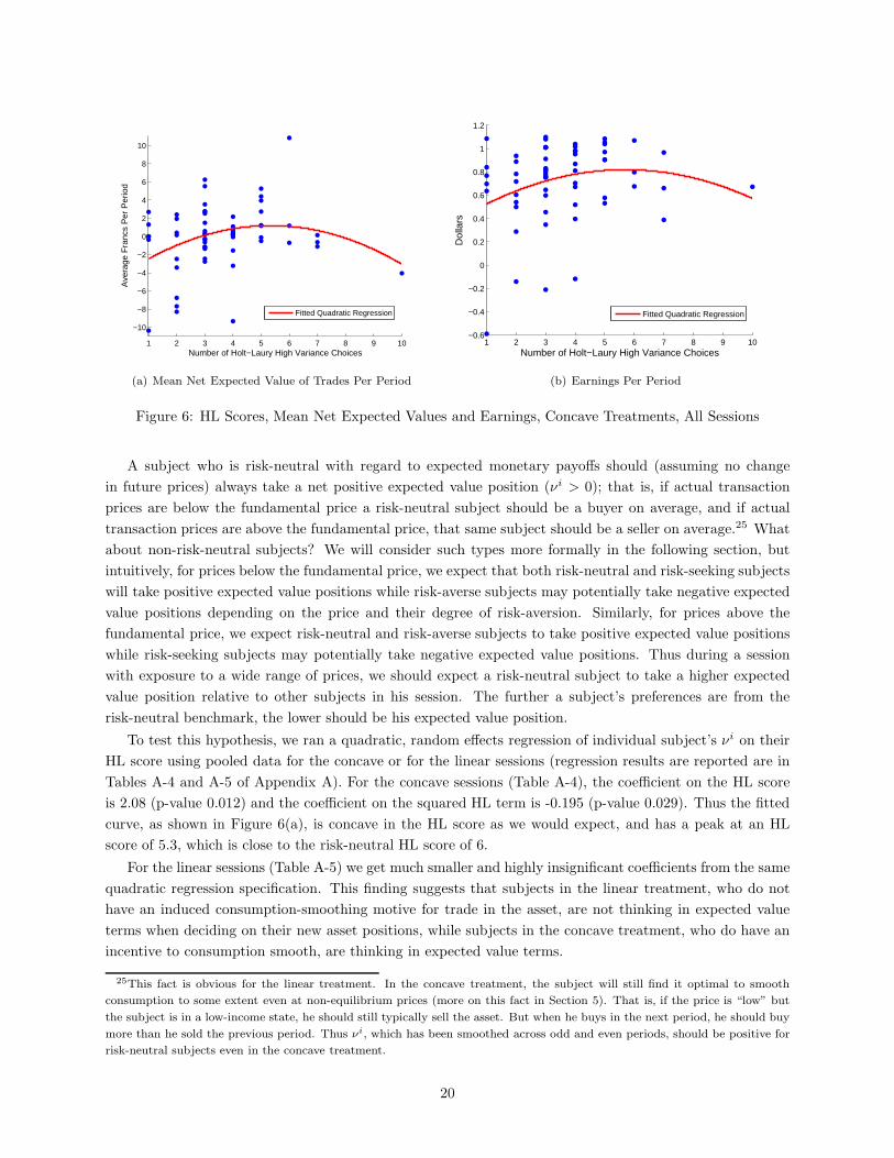
Figure 6: HL Scores, Mean Net Expected Values and Earnings, Concave Treatments, All Sessions

A subject who is risk-neutral with regard to expected monetary payoffs should (assuming no change

in future prices) always take a net positive expected value position (νi > 0); that is, if actual transaction

prices are below the fundamental price a risk-neutral subject should be a buyer on average, and if actual

transaction prices are above the fundamental price, that same subject should be a seller on average.25 What

about non-risk-neutral subjects? We will consider such types more formally in the following section, but

intuitively, for prices below the fundamental price, we expect that both risk-neutral and risk-seeking subjects

will take positive expected value positions while risk-averse subjects may potentially take negative expected

value positions depending on the price and their degree of risk-aversion. Similarly, for prices above the

fundamental price, we expect risk-neutral and risk-averse subjects to take positive expected value positions

while risk-seeking subjects may potentially take negative expected value positions. Thus during a session

with exposure to a wide range of prices, we should expect a risk-neutral subject to take a higher expected

value position relative to other subjects in his session. The further a subject’s preferences are from the

risk-neutral benchmark, the lower should be his expected value position.

To test this hypothesis, we ran a quadratic, random effects regression of individual subject’s νi on their

HL score using pooled data for the concave or for the linear sessions (regression results are reported are in

Tables A-4 and A-5 of Appendix A). For the concave sessions (Table A-4), the coefficient on the HL score

is 2.08 (p-value 0.012) and the coefficient on the squared HL term is -0.195 (p-value 0.029). Thus the fitted

curve, as shown in Figure 6(a), is concave in the HL score as we would expect, and has a peak at an HL

score of 5.3, which is close to the risk-neutral HL score of 6.

For the linear sessions (Table A-5) we get much smaller and highly insignificant coefficients from the same

quadratic regression specification. This finding suggests that subjects in the linear treatment, who do not

have an induced consumption-smoothing motive for trade in the asset, are not thinking in expected value

terms when deciding on their new asset positions, while subjects in the concave treatment, who do have an

incentive to consumption smooth, are thinking in expected value terms.

25This fact is obvious for the linear treatment. In the concave treatment, the subject will still find it optimal to smooth

consumption to some extent even at non-equilibrium prices (more on this fact in Section 5). That is, if the price is “low” but

the subject is in a low-income state, he should still typically sell the asset. But when he buys in the next period, he should buy

more than he sold the previous period. Thus νi, which has been smoothed across odd and even periods, should be positive for

risk-neutral subjects even in the concave treatment.

20

In addition to having higher net expected values, risk neutral subjects in the concave sessions also tend

to earn more than other subjects as is apparent in Figure 6(b), which shows actual mean earnings per period

as a function of subjects’ HL scores. The maximum of the fitted curve through the data depicted in Figure

6(b) is for an HL score of 5.7 (recall that risk neutrality implies an HL score of 6); regression results are

reported in Table A-6. By contrast, there is again no relationship between mean earnings per period and

HL scores in the linear treatment sessions.

5 Indigenous (homegrown) risk preferences

The HL scores indicate that a majority of subjects in our experiment are risk averse, in contrast with our

theoretical assumption of risk-neutral expected utility maximizers. It is therefore necessary for us to address

the extent to which the model’s predictions are altered by the presence of individuals with indigenous risk

aversion.

Once we alter the model to allow for indigenous risk aversion, we must make an assumption concerning

initial wealth as introduced by the term m0 in Section 2.2, as this term will matter for decision-making in

equation (6). One view of m0 is that it corresponds to the (unobserved) wealth of individual subjects at

the start of the experiment. However, as Rabin (2000) points out, it is difficult to rationalize risk aversion

over the small stakes of our experiment given the likely wealth levels that subjects have at the start of the

experiment. A second view of m0 is that it corresponds to the wealth accumulated in the experiment up to

the point of the current decision (e.g., the promised show-up payment of $5 plus earnings in all prior periods

of the experiment). A third (more myopic) view is that m0 is re-initialized to $0 at the start of every new

indefinite sequence of periods. Finally, the most extreme myopic assumption is that m0 is reset to $0 at the

start of each period.

From Rabin’s critique, we can rule out the assumption that indigenously risk averse agents set m0

equal to their actual wealth. Therefore we will consider the last three assumptions in our analysis of the

effect of initial wealth on optimization by indigenously risk-averse agents. We will maintain the (partial

equilibrium) assumption that prices are expected with certainty to remain constant at some level, p, which

greatly simplifies our analysis and allows us to focus on how the introduction of indigenous risk aversion

affects optimal behavior. Thus we can use the Euler equation (6) as our starting point. We will show that

the most straightforward way to rationalize our data is to assume extreme myopia with regard to the value

of m0.

5.1 Behavior in the Linear Treatments

We begin with the case where induced utility is linear (that is, treatments L2 and L3), so that u(c) = αc.

Recall that Mt is cumulative dollar earnings through period t, and v(m) is the subject’s indigenous utility

from m dollars, which we assume to be strictly concave (i.e., risk-averse) throughout this section. Then, by

equation (6), prices can be constant only if v′ (Mt+1) = kv′ (Mt) for all t, where k ∈ (0, 1) is a constant rate

of decay of marginal utility. Thus (6) reduces to

p =kβ

1 − kβd. (9)

Suppose subjects’ indigenous utility is characterized by the CRRA function v(m) = 11−γ

m1−γ , where

γ > 0. Then k =(

Mt

Mt+1

)γ

. Substituting this expression into (9) and applying some algebra, we obtain the

condition Mt+1 = gMt, where g =

[

(d+p)β

p

]1γ

is the optimal growth rate of wealth for period t > 1.

21

0 2 4 6 8 100

50

100

150

200

250

300

Period

Sha

res

Treatment L3, γ = 0.5, m0 = $5

Type 1 DemandType 2 DemandExcess Demand Per Pair

0 2 4 6 8 10−20

0

20

40

60

80

100

120

Period

Sha

res

Treatment L3, γ = 0.5, m0 = $0

Type 1 DemandType 2 DemandExcess Demand Per Pair

0 2 4 6 8 10−5

0

5

10

15

Period

Sha

res

Treatment L3, γ = 1, m0 = $0

Type 1 DemandType 2 DemandExcess Demand Per Pair

0 2 4 6 8 100

5

10

15

20

25

Period

Sha

res

Treatment C3, γ = 0 (risk−neutral)

Type 1 DemandType 2 DemandExcess Demand Per Pair

Figure 7: Optimal Behavior Under Constant Price p = 10

If the prevailing price p ≥ p∗ then g ≤ 1, so the subject would prefer for consumption to be zero after

the first period. Since short sales are not allowed, a risk-averse subject adopts the corner solution in which

he sells all of his shares of the asset in the first period (or as soon as possible) and simply consumes his

endowment income in subsequent periods. The behavior of many subjects was close to this prediction in the

L2 treatment (in particular, about half of the subjects held fewer than one share of the asset per period),

where prices were often above p∗.

If the prevailing price p < p∗ we have g > 1, so a risk-averse subject prefers that his wealth grows over time

at a constant rate. This growth rate is decreasing in the risk-aversion of the subject and price. Thus a more

risk-averse subject facing higher prices prefers more of his earnings earlier in the sequence and accumulates

wealth at a slower rate. For all γ > 0 (that is, for all risk-averse subjects) wealth eventually explodes as

the curvature of the subject’s indigenous utility function becomes approximately linear at “high” levels of

consumption; that is, the subject behaves approximately like a risk-neutral agent once he’s accumulated

sufficient wealth (and would prefer to borrow assets at the current price if he were allowed to borrow). Note

that it is not possible for all subjects to behave as expected utility maximizers at a constant price below p∗

because aggregate income in the experiment is constant in each period. Eventually demand would outpace

supply, causing prices to rise up toward p∗.

An important question is how quickly should we expect excess demand (and thus prices) to rise in our

experiment due to this wealth effect? Let’s focus first on the L3 treatment, where p = 10 was a commonly

observed and fairly stable price in 2 of our 4 sessions (p∗ = 15 in the L3 treatment so we have p < p∗).

Consider the behavior of a subject with γ = 0.5 (the mean degree of risk-aversion implied by our distribution

of HL scores). Suppose this subject believes that prices will continue to be 10 and further considers initial

wealth m0 to be his show-up fee, $5. The upper-left panel of Figure 7 displays the optimal shareholdings for

type 1 and type 2 subjects under these assumptions, along with their excess demand. Desired shareholdings

at the end of the first period are more than 12 for type 1 and more than 7 for type 2; thus excess demand

22

for a pair of risk-averse subjects (γ = .5) will be four times their endowment of shares at the end of the first

period alone! Thus the notion that subjects maximize utility given initial wealth earned in the experiment

(just $5) appears to be incompatible with the below-equilibrium prices observed in the two L3 sessions, at

least under the assumption of constant prices.

Suppose next that m0 = $0 at the beginning of each new sequence (so that subjects attempt to maximize

utility within each sequence independently). The upper-right panel of Figure 7 shows that our pair of

opposite-type subjects with an average degree of risk aversion (γ = .5) will now have excess demand for

shares that is nearly four times their share endowment by the fifth period. Even a pair of highly risk-averse

subjects (γ → 1, which is log utility) with m0 = $0 will have positive excess demand for shares by the

eighth period (see the lower-left panel of Figure 7). Thus regardless of the value of m0 and the degree of risk

aversion, we should not have observed stable prices as far below p∗ as we observed in some sessions of L3.

Thus it seems unlikely that subjects in the L3 sessions were attempting to dynamically optimize expected

utility when prices were consistently below p∗.26

Finally suppose that risk-averse subjects ignore wealth effects entirely, even within a sequence, i.e., m0

resets to $0 at the start of every period. In that case the Euler equation (6) is no longer binding. Under

that assumption, one can view the decision to hold an asset indefinitely as a compound lottery having an

expected value of p∗ francs. For a subject with γ = 0.5, the certainty equivalent of this compound lottery

when d = 2 is 6.9 francs, and is 10.4 francs when d = 3.27 With this view of decision-making, it is easier to

rationalize sales of assets at prices greater than or equal to these certainty equivalent values throughout a

session. Recall that prices in the L2 sessions averaged 10 or greater while prices in the L3 sessions averaged

10.3 or greater (see Table 4). Thus, a subject with a mean degree of indigenous risk aversion who ignores all

wealth effects will prefer not to buy assets at the transaction prices that prevailed on average in all sessions

of the linear treatment. Noting that nearly half of all subjects quickly sold all or nearly all of their asset

shares in the linear sessions, it appears that the assumption of extreme myopia with regard to wealth can

rationalize more of the data than can dynamic optimization of expected utility.

5.2 Behavior in the Concave Treatment

For the concave treatment, equation (6) is difficult to solve numerically for risk-averse agents.28 Thus we

will focus here on the out-of-equilibrium behavior of indigenous risk-neutral subjects in the concave induced

utility treatment and make some inferences based on that analysis for the behavior of indigenously risk-averse

subjects. In this case where agents are indigenously risk neutral, the marginal utility of indigenous wealth

becomes constant in equation (6), so that the induced marginal rate of substitution over time becomes the

only variable. Initial wealth levels don’t matter in this case.

In the lower-right panel of Figure 7 we observe optimal shareholdings for a pair of opposite type subjects

who are indigenously risk-neutral (γ = 0) and who face a constant price of 10 < p∗ = 15 (as in our C3

treatment). Desired shareholdings increase over time since p < p∗, but the optimal rate of increase is much

slower than it is for moderately risk-averse subjects (γ = 0.5) at the same price of 10 (and same p∗) when

induced preferences are linear (compare with the top two panels of Figure 7 and not the change in the scale

on the vertical axis). Thus while the risk-neutral steady state equilibrium prices of analogous linear and

concave economies are the same, optimal behavior out of equilibrium is distinctly different in the two cases.

26We are presently conducting a new stochastic horizon study where subjects can trade as much as they like in a “perfectly

competitive” market at a constant price, which will provide a rigorous test of this hypothesis.27This is the discounted expected utility of the dividend stream under the assumption of CRRA utility with γ = 0.528This is due to the interaction of the infinite sum of discounted, indigenous marginal utilities of wealth and the induced

marginal rate of substitution. To our knowledge this is a novel dynamic programming problem.

23

From Figure7 we observe that in the L3 treatment, rationally risk-averse subjects facing a below-equilibrium

price may spend early periods at a constrained outcome where they wish only to buy or sell assets. The

transition from the constrained outcome where the subject is a seller to one where he is a buyer happens very

quickly, as can be readily inferred from the first three panels of Figure 7 when coupled with the fact that

the aggregate endowment was fixed at only 5 shares per pair of subjects. This knife-edge feature of induced

linear preferences also applies to the behavioral strategy introduced above, where wealth effects within the

sequence are ignored entirely.

On the other hand, for concave induced preferences, consumption-smoothing remains a strong feature

of optimal behavior even out of equilibrium. This is apparent for the risk-neutral agents represented in the

lower-right panel of Figure 7, and we conjecture that this will also hold true for indigenously risk-averse

agents, who presumably should seek to increase their shareholdings at an even slower rate. Intuitively, the

excess demand of a pair of indigenously risk-averse agents should be bounded from above by the excess

demand of a pair of indigenously risk-neutral agents as depicted in the lower right panel of Figure 7.

We next ask whether there is a behavioral strategy analogous to the compound lottery for myopic risk-

averse subjects with concave induced preferences. Suppose subjects myopically equate the expected marginal

cost of a trade with its expected marginal benefit. Thus a type 1 subject in the first period of a sequence

would equate the marginal cost of buying ∆ shares at any price, p, in the current period with the expected

marginal benefit of those shares in the subsequent period (these shares return a dividend plus the option

value of re-sale). Assuming CRRA utility, the subject would choose ∆ such that:

[

δ + α (y2 + s1d + ∆(d + p))φ

δ + α (y1 + s1d − ∆p)φ

]γ

= −β(d + p)

p

[

y2 + s1d + ∆(d + p)

y1 + s1d − ∆p

]φ−1

(10)

The equation for a type 2 agent is similar, except this subject would set the marginal benefit of selling shares

in the current period equal to the expected marginal cost in the subsequent period.

Suppose d = 3. At the steady-state equilibrium price of p∗ = 15, all subjects following this strategy

would like to buy two shares in high income periods and sell two shares in low income periods regardless

of their degree of risk-aversion; that is, these subjects would be observationally equivalent to risk-neutral

expected utility maximizers. If p = 10, a risk-neutral type 1 subject following this behavioral strategy would

like to purchase 3 shares in the first period and sell 2.78 shares in the second period. Thus he still has a

preference to increase his shareholdings over time, but at a much slower rate than a risk-neutral expected

utility maximizer. In fact, because shares are actually discrete in our experiment, the subject would simply

prefer to cycle between buying and selling three shares.

Interestingly, this decision rule would result in nearly identical behavior regardless of the subject’s degree

of risk-aversion. For example, a type 1 subject with γ → 1 (i.e., log utility) would prefer to buy 2.94 shares

in the first period and sell 2.81 shares in the second period. In fact, if subjects follow this decision rule, the

presence of discrete asset shares implies that all prices we observe in the concave sessions are sustainable as

behavioral equilibria. It is only if prices get too low (around 60% below p∗) that we should expect to see the

least risk-averse subjects accumulate shares over time, and prices in the experiment generally remain above

this threshold.

Since prices are endogenous and typically vary within-session in our experiment, our design is ill-suited

to identify individual strategies used by subjects in the experiment. Our goal in this section is to make

it clear that optimal behavior out of equilibrium, under the simplifying assumption of constant prices, is

very different between the linear and concave treatments, and this difference is robust to intuitive behavioral

deviations from dynamic optimization of expected utility within the lab. Optimal behavior for linear induced

preferences has a knife-edge quality: Most subjects in our linear treatment should either buy or sell as many

24

shares as possible at nearly any price. Findings 4 and 5 appear to be consistent with this prediction; most

subjects sell most of their shares while a small fraction buy nearly all of the shares that are available.

Those who buy tend to be the least risk-averse subjects in the session as identified by the Holt-Laury paired

choice lottery. By contrast, optimal behavior under concave induced preferences is characterized by “thick”

markets where everyone buys or sells shares in every period, a characterization consistent with Finding 3.

Further, while large excess demand should quickly push prices to at least p∗ very quickly in the case of linear

induced preferences, substantially lower prices are consistent with “reasonable” myopic behavior in the case

of concave induced preferences.

6 Conclusion

Our research design provides an important bridge between experimental methods and experimental asset

pricing models, and the equilibrium asset pricing models used by macroeconomic/business cycle and finance

researchers. To date there has been little communication between these two fields. Our work integrating

methods and models from both fields will enable both literatures to speak to a broader audience.

What we learn from our experimental design is that an induced incentive to trade assets for the purpose

of consumption-smoothing can serve as a powerful brake on asset prices. If we loosely define a bubble as a

sustained deviation of asset prices above the fundamental price, one-half of our laboratory economies with no

induced incentive to trade the asset (the linear utility treatments) exhibited bubbles, and in three-quarters

of those sessions the bubble exhibited no signs of any collapse. Indeed, in half of the linear treatment sessions

exhibiting bubbles, the median price of the asset towards the end of the experiment was more than double the

fundamental price and was continuing to rise. In contrast, when consumption-smoothing was induced (the

concave utility treatments) in an otherwise identical economy, “bubbly” prices were observed in only one-

quarter of sessions, and in these sessions the median price of the asset had collapsed to the fundamental price

by the (random) end of the experimental session. Thus price bubbles were less frequent, of lesser magnitude,

and of shorter duration when we induced consumption-smoothing in an otherwise identical economy.

These results may offer some preliminary guidance as to which naturally occurring markets are more prone

to experience large asset price bubbles. We might reasonably expect that markets with a high concentration

of speculators, focused primarily on capital gains derived from expected price movements, are the most likely

to bubble, while markets with a large number of participants who trade at least in part for consumption-

smoothing purposes are less likely to bubble. Of course, in our current design we do not have subjects

with both linear and concave induced utility functions so at this point we merely offer the possibility that

laboratory experiments may provide the basis for such a characterization in the future.

Our experimental design can be extended in at least three distinct directions. First, the design can

be moved a step closer to the environments used in the macrofinance literature; specifically, by adding a

Markov process for dividends and/or a known, constant growth rate in endowment income. The purpose

of such treatments would be to explore the robustness of our present findings in the deterministic setting

to stochastic or growing environments. A further step would be to induce consumption-smoothing through

overlapping generations rather than via a cyclic income process and a concave exchange rate.

In another direction, it would be useful to clarify the impact of features of our experimental design relative

to the much-studied experimental design of Smith, Suchanek, and Williams (1988). For example, one could

study a finite horizon, linear (induced) utility design as in SSW, but where there exists a constant probability

of firm bankruptcy as in our present design. Would the interaction of a finite horizon but the possibility of

firm bankruptcy inhibit bubbles relative to the SSW design, or is an induced economic incentive to trade

assets necessary to prevent a small group of speculators from effectively setting asset prices across a broad

25

range of economies?

Finally, it would be useful to design an experiment to rigorously test for within-session risk preferences

and wealth effects. In our present design we observe little evidence that risk-averse subjects (classified by

the Holt-Laury paired lottery choice instrument) attempt to increase their shareholdings over time in the

linear induced utility treatment in sessions where prices are relatively low, a contradiction of time-consistent

rational risk-aversion. This result is perhaps not surprising; if subjects exhibit a different degree of risk

aversion in small stakes laboratory gambles than they apply to ‘large’ economic decisions (i.e., Rabin’s

(2000) critique), then perhaps it should be expected that they exhibit myopic risk aversion over a sequence

of small stake gambles rather than maximize expected utility globally over a sequence. To our knowledge this

hypothesis has not been directly tested. In fact, most laboratory studies of risk preferences quite consciously

and explicitly eliminate the possibility of laboratory wealth effects on subject behavior.

Modifying our present design, subjects could face a sequence of decisions to directly buy assets from or

sell assets to the experimenter at a constant price, p∗, with a constant risk of bankruptcy, i.e., we can study

individual risk preferences in a stationary, competitive market. Will risk-averse subjects (as identified by

the HL test instrument) tend to increase their shareholdings as their earnings in the experiment accumulate,

as dictated by CRRA preferences, or will their decisions be more myopic? This is an important question,

because empirical macroeconomic studies are often calibrated to a distribution of CRRA preferences as

estimated from laboratory studies. Our paper suggests the possibility that the wealth effects implied by

CRRA utility are ignored by many subjects. It is possible that an alternative to the static Holt-Laury

measure is necessary to capture the role of risk aversion in dynamic decision-making. We leave these topics

to future research.

26

References

Asparouhova, Elena, Peter Bossaerts, and Charles R. Plott (2003), “Excess Demand and Equilibration in

Multi-Security Financial Markets: The Empirical Evidence,” Journal of Financial Markets 6, 1-21.

Ballinger, T. Parker, Michael G. Palumbo and Nathanial T. Wilcox (2003), “Precautionary Savings and

Social Learning Across Generations: An Experiment,” Economic Journal 113, 920-947.

Benjamin, Daniel, Sebastian Brown, and Jesse Shapiro (2006), “Who is ‘Behavioral’? Cognitive Ability

and Anomalous Preferences,” mimeo.

Bossaerts, Peter and Charles R. Plott (2002), “The CAPM in thin experimental financial markets,” Journal

of Economic Dynamics and Control 26, 1093-1112.

Bossaerts, Peter Charles R. Plott and William R. Zame (2007), “Prices and portfolio choices in financial

markets: Theory, econometrics, experiments,” Econometrica 75, 993-1038.

Breeden, Douglas T. (1979), “An intertemporal asset pricing model with stochastic consumption and in-

vestment opportunities,” Journal of Financial Economics 7, 265–296.

Camerer, Colin and Keith Weigelt (1993), “Convergence in experimental double auctions for stochastically

lived assets,” in D. Friedman and J. Rust, Eds., The Double Auction Market: Institutions, Theories

and Evidence Cambridge, MA: Perseus Publishing, 355-396.

Carbone, Enrica and John D. Hey (2004), “The Effect of Unemployment on Consumption: An Experimental

Analysis,” Economic Journal 114, 660-683.

Cochrane, John H. (2005), Asset Pricing, Revised Edition. Princeton: Princeton University Press.

Dufwenberg, Martin, Tobias Lindqvist, and Evan Moore (2005), “Bubbles and experience: An experiment,”

American Economic Review 95, 1731-37.

Fischbacher, Urs (2007), “z-Tree: Zurich toolbox for ready-made economic experiments,” Experimental

Economics 10, 171-178.

Forsythe, Robert, Thomas Palfrey and Charles R. Plott (1982), “Asset valuation in an experimental mar-

ket,” Econometrica 50, 537-567.

Friedman, Daniel, Glenn Harrison and Jon Salmon (1984), “The informational efficiency of experimental

asset markets,” Journal of Political Economy 92, 349-408.

Hansen, Lars P., and Kenneth J. Singleton (1983), “Stochastic consumption, risk aversion and the temporal

behavior of asset returns,” Journal of Political Economy 91, 249-265.

Harrison, Glenn W., Morten I. Lau, Elisabet E. Rutstrom, and Melanie B. Sullivan, “Eliciting risk and time

preferences using field experiments: Some methodological issues,” in J. Carpenter, G.W. Harrison, and

J.A. List (eds.), Field Experiments in Economics (Greenwich, CT: JAI Press, Research in Experimental

Economics, Volume 10, 2005).

Haruvy, Ernan, Yaron Lahav and Charles N. Noussair (2007), Traders’ expectations in asset markets:

Experimental evidence. American Economic Review, 97, 1901-1920.

27

Hey, John D. and Valentino Dardanoni (1988), “Optimal consumption under uncertainty: An experimental

investigation,” Economic Journal 98, 105-116.

Holt, Charles A., and Susan K. Laury (2002), “Risk aversion and incentive effects in lottery choices,”

American Economic Review 92(5), 1644-1655.

Holt, Charles A., and Susan K. Laury (2005), “Risk aversion and incentive effects: New data without order

effects,” American Economic Review 95(3), 902-912.

Hussam, Reshmaan N., David Porter, and Vernon L. Smith “Thar she blows: Can bubbles be rekindled

with experienced subjects?” American Economic Review 98(3), 924937.

Kocherlakota, Narayana R. (1996), “The equity premium: It’s still a puzzle,” Journal of Economic Litera-

ture 34, 42-71.

Lei, Vivian, Charles N. Noussair and Charles R. Plott (2001), “Nonspeculative bubbles in experimental

asset markets: Lack of common knowledge of rationality vs. actual irrationality,” Econometrica 69,

831–59.

Lengwiler, Yvan (2004), Microfoundations of Financial Economics, Princeton: Princeton University Press.

LeRoy, Stephen F. and Richard D. Porter (1981), “The present value relation: Tests based on implied

variance bounds,” Econometrica, 49, 555—574.

Lucas, Robert E. Jr., (1978), “Asset prices in an exchange economy,” Econometrica 46, 1429–1445.

Lugovskyy, Volodymyr, Daniela Puzzello, and Steven Tucker (2010), “An experimental study of bubble

formation in asset markets using the tatonnement pricing mechanism,” mimeo.

Mankiw, N. Gregory and Stephen P. Zeldes, (1991), “The consumption of stockholders and nonstockhold-

ers,” Journal of Financial Economics, 29, 97-112.

Noussair, Charles N. and Kenneth J. Matheny (2000), “An experimental study of decisions in dynamic

optimization problems,” Economic Theory 15, 389-419

Plott, Charles R. and Vernon L. Smith (2008), Eds., Handbook of Experimental Economic Results Vol.1,

Amsterdam: North Holland.

Plott, Charles R. and S. Sunder (1982), “Efficiency of experimental security markets with insider trading,”

Journal of Political Economy 90, 663-698.

Porter, David P. and Vernon L. Smith (1995), “Futures contracting and dividend uncertainty in experi-

mental asset markets,” Journal of Business 68, 509-541.

Rabin, Matthew (2000), “Diminishing Marginal Utility of Wealth Cannot Explain Risk Aversion,” in

Choices, Values, and Frames, edited by Daniel Kahneman and Amos Tversky, New York: Cambridge

University Press, 202-208.

Roth, Alvin and J. Keith Murnighan (1978), “Equilibrium behavior and repeated play of the prisoners’

dilemma,” Journal of Mathematical Psychology, 17, 189-198.

Shiller, Robert J. (1981), Do stock prices move too much to be justified by subsequent changes in dividends?”

American Economic Review, 71, 421—436.

28

Smith, Vernon L. (1962), “An experimental study of competitive market behavior,” Journal of Political

Economy 70, 111-137.

Smith, Vernon L., Gerry L. Suchanek, and Arlington W. Williams (1988), “Bubbles, crashes and endogenous

expectations in experimental spot asset markets,” Econometrica 56, 1119-51.

Stiglitz, Joseph E. (1970), “A consumption-oriented theory of the demand for financial assets and the term

structure of interest rates,” Review of Economic Studies 37, 321-351.

Wheatley, S. (1988), “Some tests of the consumption-based asset pricing model,” Journal of Monetary

Economics 22, 193—215.

29

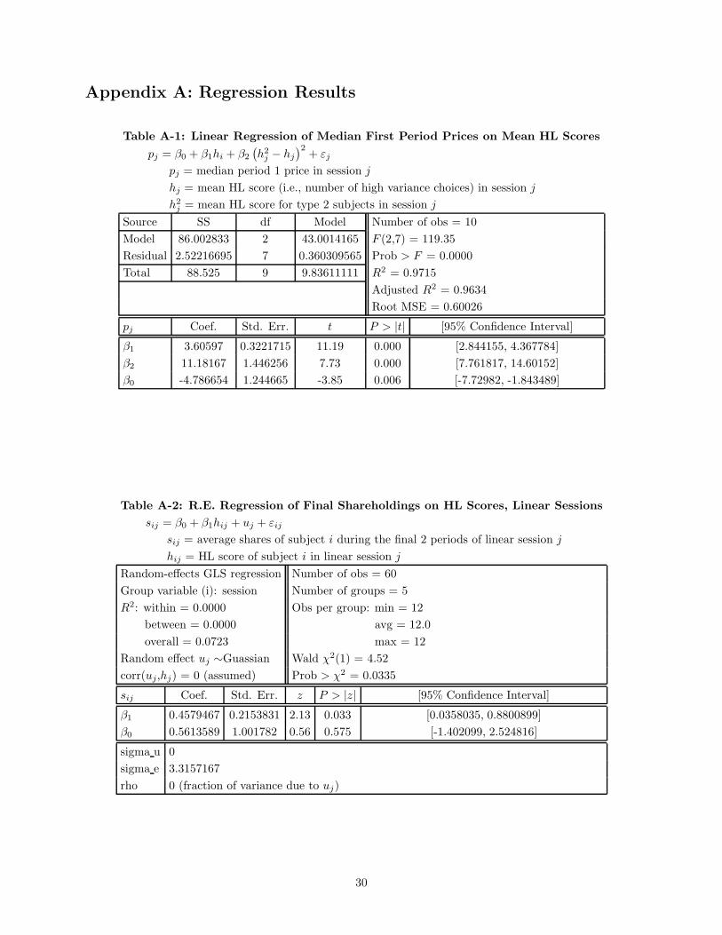
Appendix A: Regression Results

Table A-1: Linear Regression of Median First Period Prices on Mean HL Scores

pj = β0 + β1hi + β2

(

h2j − hj

)2+ εj

pj = median period 1 price in session j

hj = mean HL score (i.e., number of high variance choices) in session j

h2j = mean HL score for type 2 subjects in session j

Source SS df Model Number of obs = 10

Model 86.002833 2 43.0014165 F (2,7) = 119.35

Residual 2.52216695 7 0.360309565 Prob > F = 0.0000

Total 88.525 9 9.83611111 R2 = 0.9715

Adjusted R2 = 0.9634

Root MSE = 0.60026

pj Coef. Std. Err. t P > |t| [95% Confidence Interval]

β1 3.60597 0.3221715 11.19 0.000 [2.844155, 4.367784]

β2 11.18167 1.446256 7.73 0.000 [7.761817, 14.60152]

β0 -4.786654 1.244665 -3.85 0.006 [-7.72982, -1.843489]

Table A-2: R.E. Regression of Final Shareholdings on HL Scores, Linear Sessions

sij = β0 + β1hij + uj + εij

sij = average shares of subject i during the final 2 periods of linear session j

hij = HL score of subject i in linear session j

Random-effects GLS regression Number of obs = 60

Group variable (i): session Number of groups = 5

R2: within = 0.0000 Obs per group: min = 12

between = 0.0000 avg = 12.0

overall = 0.0723 max = 12

Random effect uj ∼Guassian Wald χ2(1) = 4.52

corr(uj,hj) = 0 (assumed) Prob > χ2 = 0.0335

sij Coef. Std. Err. z P > |z| [95% Confidence Interval]

β1 0.4579467 0.2153831 2.13 0.033 [0.0358035, 0.8800899]

β0 0.5613589 1.001782 0.56 0.575 [-1.402099, 2.524816]

sigma u 0

sigma e 3.3157167

rho 0 (fraction of variance due to uj)

30

Table A-3: R.E. Regression of Final Shareholdings on HL Scores, Concave Sessions

sij = β0 + β1hij + uj + εij

sij = average shares of subject i during the final 2 periods of concave session j

hij = HL score of subject i in concave session j

Random-effects GLS regression Number of obs = 60

Group variable (i): session Number of groups = 5

R2: within = 0.0000 Obs per group: min = 12

between = 0.0000 avg = 12.0

overall = 0.0117 max = 12

Random effect uj ∼Guassian Wald χ2(1) = 0.69

corr(uj,hj) = 0 (assumed) Prob > χ2 = 0.4074

sij Coef. Std. Err. z P > |z| [95% Confidence Interval]

β1 -0.0969082 0.1169705 -0.83 0.407 [0.3261662, 0.1323499]

β0 2.847254 0.4656838 6.11 0.000 [1.934531, 3.759978]

sigma u 0

sigma e 1.6286249

rho 0 (fraction of variance due to uj)

Table A-4: R.E. Quadratic Regression, Net E.V. Positions on HL Scores, Concave Sessions

νij = β0 + β1hij + β2h2ij + uj + εij

νij = mean expected value position of subject i in concave session j

hij = HL score of subject i in concave session j

Random-effects GLS regression Number of obs = 60

Group variable (i): session Number of groups = 5

R2: within = 0.1093 Obs per group: min = 12

between = 0.1738 avg = 12.0

overall = 0.1049 max = 12

Random effect uj ∼Guassian Wald χ2(1) = 6.68

corr(uj,hj) = 0 (assumed) Prob > χ2 = 0.0355

vij Coef. Std. Err. z P > |z| [95% Confidence Interval]

β1 2.08459 0.8316107 2.51 0.012 [0.4546632, 3.714517]

β2 -0.1953346 0.0891952 -2.19 0.029 [-0.370154, -0.0205152]

β0 -4.373728 1.750486 -2.50 0.012 [-7.804617, -0.9428389]

sigma u 0

sigma e 3.5726936

rho 0 (fraction of variance due to uj)

31

Table A-5: R.E. Quadratic Regression, Net E.V. Positions on HL Scores, Linear Sessions

νij = β0 + β1hij + β2h2ij + uj + εij

νij = mean expected value position of subject i in linear session j

hij = HL score of subject i in linear session j

Random-effects GLS regression Number of obs = 60

Group variable (i): session Number of groups = 5

R2: within = 0.0009 Obs per group: min = 12

between = 0.0127 avg = 12.0

overall = 0.0009 max = 12

Random effect uj ∼Guassian Wald χ2(1) = 0.05

corr(uj,hj) = 0 (assumed) Prob > χ2 = 0.9751

vij Coef. Std. Err. z P > |z| [95% Confidence Interval]

β1 -0.049834 0.6942685 -0.07 0.943 [-1.410575, 1.310907]

β2 0.0084909 0.0651754 0.13 0.896 [-0.1192505, 0.1362323]

β0 0.02728 1.685973 0.02 0.987 [-3.277166, 3.331726]

sigma u 0

sigma e 3.1090359

rho 0 (fraction of variance due to uj)

Table A-6: R.E. Quadratic Regression of Period Earnings on HL Scores, Concave Sessions

dij = β0 + β1hij + β2h2ij + uj + εij

dij = mean dollars per period earned by subject i in concave session j

hij = HL score of subject i in concave session j

Random-effects GLS regression Number of obs = 60

Group variable (i): session Number of groups = 5

R2: within = 0.0732 Obs per group: min = 12

between = 0.0018 avg = 12.0

overall = 0.0641 max = 12

Random effect uj ∼Guassian Wald χ2(1) = 4.23

corr(uj,hj) = 0 (assumed) Prob > χ2 = 0.1205

dij Coef. Std. Err. z P > |z| [95% Confidence Interval]

β1 0.1479577 0.079462 1.86 0.063 [-0.0077849, 0.3037003]

β2 -0.0128485 0.0085561 -1.50 0.133 [-0.029618, 0.0039211]

β0 0.3932561 0.1736306 2.26 0.024 [0.0529465, 0.7335658]

sigma u 0.11107893

sigma e 0.33065127

rho 0.10141079 (fraction of variance due to uj)

32

Appendix B: Instructions Used in the Experiment

The instructions distributed to subjects in the C2 treatment are reproduced on the following pages. Sub-

jects in the C3 treatment received identical instructions, except that dividends were changed from 2 to 3

throughout. Subjects in the L2 and L3 treatments received identical instructions to their counterparts in C2

and C3, respectively, except for the fourth paragraph. The modified fourth paragraph in the instructions for

the L2 and L3 treatments is reproduced at the end of the C2 treatment instructions.

Following these instructions we present a reproduction of the endowment sheets, payoff tables, and payoff

charts for all subjects. After these supplements we present the instructions distributed to all subjects for the

Holt-Laury paired-choice lottery. A complete set of all instructions used in all treatments of this experiment

can be found at http://www.pitt.edu/∼jduffy/assetpricing.

33

Experimental Instructions

I. Overview

This is an experiment in the economics of decision making. If you follow the instructions

carefully and make good decisions you may earn a considerable amount of money that will

be paid to you in cash at the end of this session. Please do not talk with others for the

duration of the experiment. If you have a question please raise your hand and one of the

experimenters will answer your question in private.

Today you will participate in one or more “sequences”, each consisting of a number of

“trading periods”. There are two objects of interest in this experiment, francs and assets.

At the start of each period you will receive the number of francs as indicated on the page

entitled “Endowment Sheet”. In addition, you will earn 2 francs for each unit of the asset

you hold at the start of a period (please look at the endowment sheet now). During the

period you may buy assets from or sell assets to other participants using francs. Details

about how this is done are discussed below in section IV.

At the end of each period, your end-of-period franc balance will be converted into dollar

earnings. These dollar earnings will accumulate across periods and sequences, and will be

paid to you in cash at the end of the experiment. The number of assets you own carry

over from one period to the next, if there is a next period (more on this below), whereas

your end-of-period franc balance does not -you start each new period with the endowment of

francs indicated on your Endowment Sheet. Therefore, there are two reasons to hold assets:

(1) they provide additional francs at the beginning of each period and (2) assets may be sold

for francs in some future period.

Please open your folder and look at the “Payoff Table” showing how your end-of-period franc

balance converts into dollars. The “Payoff Chart” provides a graphical illustration of the

payoff table. There are several things to notice. First, very low numbers of francs yield

negative dollar payoffs. The lowest number in the payoff table is 11 francs. You are not

permitted to hold less than 11 francs at any time during the experiment. Second, the more

francs you earn in a period, the higher will be your dollar earnings for that period. Finally,

the dollar payoff from each additional franc that you earn in a period is diminishing; for

example, the payoff difference between 56 and 57 francs is larger than the difference between

93 and 94 francs.

NOTE: The total number of francs and assets held by all participants in this market does

not change over the course of a sequence. Further, the number of francs provided by each

asset, 2, is the same for all participants.

34

II. Preliminary Quiz

Using your endowment sheet and payoff table, we now pause and ask you to answer the

following questions. We will come around to verify that your answers are correct.

1. Suppose it is the first period of a sequence (an odd-numbered period). What is the

number of assets you own?

2. What is the total number of francs you have available at the start of the first period,

including both your endowment of francs and the 2 francs you get for each unit of the asset

you own at the start of the period?

3. Suppose that at the end of the first period you have not bought or sold any assets, so

your franc total is the same as at the start of the period (your answer to question 2). What

is your payoff in dollars for this first period?

4. Suppose that the sequence continues with period 2 (an even-numbered period), and that

you did not buy or sell any assets in the first period, so you own the same number of assets.

What is the total number of francs you have available at the start of period 2, including

both your endowment of francs and the 2 francs you get for each unit of the asset you own

at the start of a period?

5. Suppose again that at the end of period 2 you have not bought or sold any assets, so

your franc total is the same as at the start of the period (your answer to question 4). What

is your payoff in dollars for this second period? What would be your

dollar earnings in the sequence to this point?

III: Sequences of Trading Periods

As mentioned, today’s session consists of one or more “sequences,” with each sequence con-

sisting of a number of “periods.” Each period lasts 3 minutes. At the end of each period your

end-of-period franc balance, dollar payoff and the number of assets will be shown to you on

your computer screen. One of the participants will then roll a die (with sides numbered from

1-6). If the number rolled is 1-5, the sequence will continue with a new, 3-minute period.

If a 6 is rolled, the sequence will end and your cash balance for that sequence will be final.

Any assets you own will become worthless. Thus, at the start of each period, there is a 1 in

6 (or about 16.7 percent) chance that the period will be the last one played in the sequence

and a 5 in 6 (or about 83.3 percent) chance that the sequence will continue with another

period.

If less than 60 minutes have passed since the start of the first sequence, a new sequence will

begin. You will start the new sequence and every new sequence just as you started the first

35

sequence, with the number of francs and assets as indicated on your endowment sheet. The

quantity of francs you receive in each period will alternate as before, between odd and even

periods, and the total number of assets available for sale (across all participants) will remain

constant in every period of the sequence. If more than 60 minutes has elapsed since the

beginning of the first sequence then the current sequence will be the last sequence played;

that is, the next time a 6 is rolled the sequence will end and the experiment will be over.

The total dollar amount you earned from all sequences will be calculated and you will be

paid this amount together with your $5 show-up fee in cash and in private before exiting the

room.

If, by chance, the final sequence has not ended by the three-hour period for which you have

been recruited, we will schedule a continuation of this sequence for another time in which

everyone here can attend. You would be immediately paid your earnings from all sequences

that ended in today’s session. You would start the continuation sequence with the same

number of assets you ended with in today’s session, and your franc balance would continue

to alternate between odd and even periods as before. You would be paid your earnings for

this final sequence after it has been completed.

IV. Asset Trading Rules

During each three minute (180 second) trading period, you may choose to buy or sell assets.

Trade happens on the trading window screen, show below. The current period is shown in

the upper left and the time remaining for trading in this period (in seconds) is indicated in

the upper right. The number of francs and assets you have available is shown on the left.

Assets are bought and sold one unit at a time, but you can buy or sell more than one unit

in a trading period.

To submit a bid or buying price for an asset, type in the amount of francs you are willing to

pay for a unit of the asset in the “Buying price” box on the right. Then click on the “Post

Buying Price” button on the bottom right. The computer will tell you if you don’t have

enough francs to place a buy order; recall that you cannot go below a minimum of 11 francs

in your account. Once your buy price has been submitted, it is checked against any other

existing buy prices. If your buy price is higher than any existing buy price, it will appear

under the “Buying Price” column in the middle right of the screen; otherwise, you will be

asked to revise your bid upward - you must improve on existing bids. Once your buy price

appears on the trading screen, any player who has a unit of the asset available can choose

to sell it to you at that price by using the mouse to highlight your buy price and clicking on

the button “Sell at Highest Price” (bottom center-right of the screen). If that happens, the

number of francs you bid is transferred to the seller and one unit of the asset is transferred

36

from the seller to you. Another possibility is that another person will choose to improve on

the buy price you submitted by entering a higher buy price. In that case, you must increase

your buy price even higher to have a chance of buying the asset.

Trading Window Screen

To submit a selling or “ask” price for an asset, type in the amount of francs you would be

willing to accept to sell an asset in the “Selling offer” box on the left and then click the

“Post Selling Price” button on the bottom left. Note: you cannot sell an asset if you do

not presently have an asset available to sell in your account. Once your sell price has been

submitted, it is checked against any other existing sell prices. If your sell price is lower

than any existing sell prices, it will appear on the trading screen under the ”Selling Price”

column in the middle left of the screen; otherwise, you will be asked to revise your sell price

downward - you must improve on existing offers to sell. Any participant who has enough

francs available can choose to buy the asset from you at your price by using the mouse to

highlight your sell price and clicking on the button labeled ”Buy at Lowest Price” (bottom

center-left of the screen). If that happens, one unit of the asset is transferred from you to the

buyer, and in exchange the number of francs you agreed to sell the asset for is transferred

37

from the buyer to you. Another possibility is that another person will choose to improve on

the sell price you submitted, by entering an even lower sell price. In that case, you will have

to lower your sell price even further to have a chance of selling the asset.

Whenever an agreement to buy/sell between any two players takes place, the transaction

price is shown in the middle column of the trading screen labeled “Transaction Price.” If

someone has chosen to buy at the lowest price, all selling prices are cleared from the trading

screen. If someone has chosen to sell at the highest price, all buying prices are cleared from

the trading screen. As long as trading remains open, you can post new buy and sell prices

and agree to make transactions following the same rules given above. The entire history of

transaction prices will remain in the middle column for the duration of each trading period.

At the end of each period, you will be told your end-of-period franc balance and dollar payoff

for the period, along with your cumulative total dollar payoff over all periods played in the

sequence thus far. At then end of each sequence (whenever a “6” is rolled), we will ask you

to write down, on your earnings sheet, the sequence number, the number of trading periods

in that sequence and your total dollar payoff for that sequence.

V. Final Quiz

Before continuing on to the experiment, we ask that you consider the following scenarios and

provide answers to the questions asked in the spaces provided. The numbers used in this

quiz are merely illustrative; the actual numbers in the experiment may be quite different.

You will need to consult your payoff table to answer some of these questions.

Question 1: Suppose that a sequence has reached period 15. What is the chance that this

sequence will continue with another period - period 16? . Would your

answer be any different if we replaced 15 with 5 and 16 with 6? Circle one: yes / no.

Question 2: Suppose a sequence ends (a 6 is rolled) and you have n assets. What is the

value of those n assets? . Suppose instead, the sequence continued

into another period (a 1-5 is rolled)-how many assets would you hold in the next period?

.

For questions 3-6 below: suppose at the start of this period you are given 70 francs. In

addition, you own 3 assets.

Question 3: What is the maximum number of assets you can sell at the start of the 3-minute

trading period? .

Question 4: What is the total number of francs you will have available at the start of the

trading period (including francs from assets owned)? . If you do not

38

buy or sell any assets during the 3-minute trading period, what would be your end-of-period

dollar payoff? .

Question 5: Now suppose that, during the 3-minute trading period, you sold 2 of your 3

assets: specifically, you sold one asset for a price of 4 francs and the other asset for a price of

8 francs. What is your end-of-period franc total in this case? . What

would be your dollar payoff for the period? . What is the number of

assets you would have at the start of the next period (if there is one)? .

Question 6: Suppose that instead of selling assets during the trading period (as in question

5), you instead bought one more asset at a price of 18 francs. What would be your end-of-

period franc total in this case? . What would be your dollar payoff for

the period? . What is the number of assets you will have at the start

of the next period (if there is one)? .

VI. Questions

Now is the time for questions. If you have a question about any aspect of the instructions,

please raise your hand.

What follows below is the fourth paragraph of the instructions for subjects in the L2 and L3

treatments.

Please open your folder and look at the “Payoff Table” showing how your end-of-period

franc balance converts into dollars. The “Payoff Chart” provides a graphical illustration of

the payoff table. There are several things to notice. First, the lowest number in the payoff

table is 11 francs. You are not permitted to hold less than 11 francs at any time during

the experiment. Second, the more francs you earn in a period, the higher will be your dollar

earnings for that period. Finally, the dollar payoff from each additional franc that you earn

in a period is the same; the formula for converting between francs and dollars is fixed and is

given at the bottom of your table.

39

ENDOWMENT SHEET[Not visible to subjects: Type 1 subject, d = 2]

This information is private. Please do

not share with others.

Initial franc balance in all odd periods (first,

third, fifth, etc.): 110

Initial franc balance in all even periods (second,

fourth, sixth, etc.): 44

Assets you own in the first period: 1

Francs paid per asset at start of each period: 2

Therefore, you will begin the first period with

110 + 1*2 = 112 francs

40

ENDOWMENT SHEET[Not visible to subjects: Type 2 subject, d = 2]

This information is private. Please do

not share with others.

Initial franc balance in all odd periods (first,

third, fifth, etc.): 24

Initial franc balance in all even periods (second,

fourth, sixth, etc.): 90

Assets you own in the first period: 4

Francs paid per asset at start of each period: 2

Therefore, you will begin the first period with

24 + 4*2 = 32 francs

41

ENDOWMENT SHEET[Not visible to subjects: Type 1 subject, d = 3]

This information is private. Please do

not share with others.

Initial franc balance in all odd periods (first,

third, fifth, etc.): 110

Initial franc balance in all even periods (second,

fourth, sixth, etc.): 44

Assets you own in the first period: 1

Francs paid per asset at start of each period: 3

Therefore, you will begin the first period with

110 + 1*3 = 113 francs

42

ENDOWMENT SHEET[Not visible to subjects: Type 2 subject, d = 3]

This information is private. Please do

not share with others.

Initial franc balance in all odd periods (first,

third, fifth, etc.): 24

Initial franc balance in all even periods (second,

fourth, sixth, etc.): 90

Assets you own in the first period: 4

Francs paid per asset at start of each period: 3

Therefore, you will begin the first period with

24 + 4*3 = 36 francs

43

[Not visible to subjects: Type 1 subject, concave treatments (C2 and C3)]

44

[Not visible to subjects: Type 1 subject, concave treatments (C2 and C3)]

45

[Not visible to subjects: Type 2 subject, concave treatments (C2 and C3)]

46

[Not visible to subjects: Type 2 subject, concave treatments (C2 and C3)]

47

[Not visible to subjects: Type 1 subject, linear treatments (L2 and L3)]

48

[Not visible to subjects: Type 1 subject, linear treatments (L2 and L3)]

49

[Not visible to subjects: Type 2 subject, linear treatments (L2 and L3)]

50

[Not visible to subjects: Type 2 subject, linear treatments (L2 and L3)]

51

Instructions [Not visible to subjects: Holt-Laury Procedure

You will face a sequence of 10 decisions. Each decision is a paired choice between two options, labeled

“Option A” and “Option B”. For each decision you must choose either Option A or Option B. You do this

by clicking next to the radio button corresponding to your choice on the computer screen. After making

your choice, please also record it on the attached record sheet under the appropriate headings.

The sequence of 10 decisions you will face are as follows:

Decision Option A Option B

1 Receive $6.00 10 out of 100 draws OR Receive $11.55 10 out of 100 draws OR

Receive $4.80 90 out of 100 draws Receive $ 0.30 90 out of 100 draws

2 Receive $6.00 20 out of 100 draws OR Receive $11.55 20 out of 100 draws OR

Receive $4.80 80 out of 100 draws Receive $ 0.30 80 out of 100 draws

3 Receive $6.00 30 out of 100 draws OR Receive $11.55 30 out of 100 draws OR

Receive $4.80 70 out of 100 draws Receive $ 0.30 70 out of 100 draws

4 Receive $6.00 40 out of 100 draws OR Receive $11.55 40 out of 100 draws OR

Receive $4.80 60 out of 100 draws Receive $ 0.30 60 out of 100 draws

5 Receive $6.00 50 out of 100 draws OR Receive $11.55 50 out of 100 draws OR

Receive $4.80 50 out of 100 draws Receive $ 0.30 50 out of 100 draws

6 Receive $6.00 60 out of 100 draws OR Receive $11.55 60 out of 100 draws OR

Receive $4.80 40 out of 100 draws Receive $ 0.30 40 out of 100 draws

7 Receive $6.00 70 out of 100 draws OR Receive $11.55 70 out of 100 draws OR

Receive $4.80 30 out of 100 draws Receive $ 0.30 30 out of 100 draws

8 Receive $6.00 80 out of 100 draws OR Receive $11.55 80 out of 100 draws OR

Receive $4.80 20 out of 100 draws Receive $ 0.30 20 out of 100 draws

9 Receive $6.00 90 out of 100 draws OR Receive $11.55 90 out of 100 draws OR

Receive $4.80 10 out of 100 draws Receive $ 0.30 10 out of 100 draws

10 Receive $6.00 100 out of 100 draws OR Receive $11.55 100 out of 100 draws OR

Receive $4.80 0 out of 100 draws Receive $ 0.30 0 out of 100 draws

After you have made all 10 decisions, the computer program will randomly select 1 of the 10 decisions and

your choice for that decision will be used to determine your payoff. All 10 decisions have the same chance

of being chosen.

Notice that for each decision, the two options describe two different amounts of money you can receive,

depending on a random draw. The random draw will be made by the computer and will be a number

(integer) from 1 to 100 inclusive. Consider Decision 1. If you choose Option A, then you receive $6.00 if the

random number drawn is 10 or less, that is, in 10 out of 100 possible random draws made by the computer,

or 10 percent of the time, while you receive $4.80 if the random number is between 11 and 100, that is in 90

out of 100 possible random draws made by the computer, or 90 percent of the time. If you choose Option B,

then you receive $11.55 if the random number drawn is 10 or less, that is, in 10 out of 100 possible random

draws made by the computer, while you receive $0.30 if the random number is between 11 and 100, that is

in 90 out of 100 possible random draws made by the computer, or 90 percent of the time. Other decisions

are similar, except that your chances of receiving the higher payoff for each option increase. Notice that all

decisions except decision 10 involve random draws. For decision 10, you face a certain (100 percent) chance

52

of $6.00 if you choose Option A or a certain (100 percent) chance of $11.55 if you choose Option B.

Even though you make 10 decisions, only ONE of these decisions will be used to determine your earnings

from this experiment. All 10 decisions have an equal chance of being chosen to determine your earnings.

You do not know in advance which of these decisions will be selected.

Consider again decision 1. This will appear to you on your computer screen as follows:

The pie charts help you to visualize your chances of receiving the two amounts presented by each option.

When you are ready to make a decision, simply click on the button below the option you wish to choose.

Please also circle your choice for each of the 10 decisions on your record sheet. When you are satisfied with

your choice, click the Next button to move on to the next decision. You may choose Option A for some

decisions and Option B for others and you may change your decisions or make them in any order using the

Previous and Next buttons.

When you have completed all 10 choices, and you are satisfied with those choices you will need to click

the Confirm button that appears following decision 10. The program will check that you have made all 10

decisions; if not, you will need to go back to any incomplete decisions and complete those decisions which you

can do using the Previous button. You can also go back and change any of your decisions prior to clicking

the confirm button by using the Previous button.

Once you have made all 10 decisions and clicked the Confirm button, the results screen will tell you the

decision number 1, 210, that was randomly selected by the computer program. Your choice of option A or

B for that decision (and that decision only) will then be used to determine your dollar payoff. Specifically,

the computer will draw a random number between 1 and 100 (all numbers have an equal chance) and report

to you both the random number drawn and the payoff from your option choice.

Your payoff will be added to the amount you have already earned in today’s experiment. Please circle the

decision that was chosen for payment on your record sheet and write down both the random number drawn

by the computer program and the amount you earned from the option you chose for that decision on your

record sheet. On the computer monitor, type in your subject ID number, which is the same number used to

identify you in the first experiment in today’s session. Then click the ”Save and Close” button.

Are there any questions before we begin?

53

Please do not talk with anyone while these decisions are being made. If you have a question while making

decisions, please raise your hand.

Record Sheet Player ID Number

Circle Option Choice

Decision 1 A B

Circle Option Choice

Decision 2 A B

Circle Option Choice

Decision 3 A B

Circle Option Choice

Decision 4 A B

Circle Option Choice

Decision 5 A B

Circle Option Choice

Decision 6 A B

Circle Option Choice

Decision 7 A B

Circle Option Choice

Decision 8 A B

Circle Option Choice

Decision 9 A B

Circle Option Choice

Decision 10 A B

At the end of this experiment, circle the Decision number selected by the computer program for payment.

Write down the random number drawn for the selected decision (between 1 and 100):

Write down your payment earned for this part of the experiment: $

54