a dynamic control approach to modeling and analysing the e

A Dynamic Control Approach toModeling and Analysing the Effects

of Rewards on Behaviour andAttitude Change

by

Elizabeth Vanderwater

A thesispresented to the University of Waterloo

in fulfillment of thethesis requirement for the degree of

Master of Applied Sciencein

Electrical and Computer Engineering

Waterloo, Ontario, Canada, 2010

c© Elizabeth Vanderwater 2010

I hereby declare that I am the sole author of this thesis. This is a true copy of the thesis,including any required final revisions, as accepted by my examiners.

I understand that my thesis may be made electronically available to the public.

ii

Abstract

Motivated by the dynamic feedback nature of human attitudes and behaviours, this workadopts a control systems engineering approach to studying a psychological system. In par-ticular, two discrete-time nonlinear attitude-behaviour models are developed to describehow rewards influence a person’s attitude and behaviour. The first model arises from threewell-established social psychological theories: the theory of planned behaviour, cognitivedissonance theory and the overjustification effect. This model, called the one-person sys-tem, consists of a single person who is influenced (in a controlling manner) by a reward.The second model, called the two-person system, consists of two people, one of whom isinfluenced by a reward, and is obtained by extending the framework of the one-personsystem to incorporate the additional influence exerted by the behaviours of other people.Many interesting control problems arise for these two systems; this work focuses on theproblem of finding a sequence of reward values that is capable of forcing the behaviour ofa person (who has an initially negative attitude) to a certain, positive value. Open-loopand closed-loop controllers are designed to meet this control objective and simulations areused to confirm the functionality of these controllers. Additionally, throughout the systemanalysis, psychological predictions made by the models that may be of interest to socialpsychologists are highlighted.

iii

Acknowledgements

I would like to thank my supervisor, Professor Daniel Davison, for his support andguidance. I would also like to thank Professors Kulic and Nielsen for their comments onthis thesis. Finally, I would like to thank my family and friends for their endless patienceand encouragement.

iv

Contents

List of Tables x

List of Figures xiii

1 Introduction 1

1.1 Motivation . . . . . . . . . . . . . . . . . . . . . . . . . . . . . . . . . . . . 1

1.2 Problem Statement . . . . . . . . . . . . . . . . . . . . . . . . . . . . . . . 3

1.3 Contributions . . . . . . . . . . . . . . . . . . . . . . . . . . . . . . . . . . 5

1.4 Thesis Overview . . . . . . . . . . . . . . . . . . . . . . . . . . . . . . . . . 6

2 One-Person System:Psychology and Modelling 7

2.1 Psychology Describing How AttitudesDrive Behaviour . . . . . . . . . . . . . . . . . . . . . . . . . . . . . . . . . 8

2.1.1 Background . . . . . . . . . . . . . . . . . . . . . . . . . . . . . . . 8

2.1.2 Theory of Planned Behaviour . . . . . . . . . . . . . . . . . . . . . 8

2.2 Psychology Describing How BehaviourDrives Attitudes . . . . . . . . . . . . . . . . . . . . . . . . . . . . . . . . . 12

2.2.1 Cognitive Dissonance Theory:Overview . . . . . . . . . . . . . . . . . . . . . . . . . . . . . . . . 13

2.2.2 Cognitive Dissonance Theory:Induced Compliance Paradigm . . . . . . . . . . . . . . . . . . . . . 14

2.2.3 The Overjustification Effect . . . . . . . . . . . . . . . . . . . . . . 17

2.3 A Dynamic Attitude-Behaviour Model . . . . . . . . . . . . . . . . . . . . 18

v

2.3.1 Details of Component A . . . . . . . . . . . . . . . . . . . . . . . . 20

2.3.2 Details of Component B . . . . . . . . . . . . . . . . . . . . . . . . 20

2.3.3 Simplifying Assumptions and Initial Conditions . . . . . . . . . . . 23

2.3.4 Interpreting the Discrete-Time Model . . . . . . . . . . . . . . . . . 24

2.4 Model Consistency Verification . . . . . . . . . . . . . . . . . . . . . . . . 26

3 One-Person System:Simulation and Control Strategies 36

3.1 Open-Loop Investigation . . . . . . . . . . . . . . . . . . . . . . . . . . . . 36

3.1.1 Impulse-Reward Controller Design . . . . . . . . . . . . . . . . . . 36

3.1.2 Step-Reward Controller Design . . . . . . . . . . . . . . . . . . . . 43

3.2 Closed-Loop Investigation . . . . . . . . . . . . . . . . . . . . . . . . . . . 46

3.2.1 State-Feedback Controllers . . . . . . . . . . . . . . . . . . . . . . . 47

3.2.2 Output-Feedback Controller Design . . . . . . . . . . . . . . . . . . 52

3.2.3 Output-Feedback Controller Analysis . . . . . . . . . . . . . . . . . 62

4 Two-Person System:Psychology and Modelling 75

4.1 Psychology Describing the Influence ofOther People . . . . . . . . . . . . . . . . . . . . . . . . . . . . . . . . . . 76

4.1.1 Social Pressure . . . . . . . . . . . . . . . . . . . . . . . . . . . . . 76

4.1.2 Conformity Pressure . . . . . . . . . . . . . . . . . . . . . . . . . . 78

4.2 The Augmented Dynamic Feedback Model . . . . . . . . . . . . . . . . . . 80

4.2.1 Revising Component A . . . . . . . . . . . . . . . . . . . . . . . . . 83

4.2.2 Revising Component B . . . . . . . . . . . . . . . . . . . . . . . . . 83

4.2.3 Simplifying Assumptions and Initial Conditions . . . . . . . . . . . 87

4.3 Model Consistency Verification . . . . . . . . . . . . . . . . . . . . . . . . 89

4.3.1 Social Pressure Consistency Verification . . . . . . . . . . . . . . . 89

4.3.2 Conformity Pressure Consistency Verification . . . . . . . . . . . . 92

4.4 Other Psychological Phenomena . . . . . . . . . . . . . . . . . . . . . . . . 95

vi

5 Two-Person System:Simulation and Control Strategies 99

5.1 Zero-Input Response Analysis . . . . . . . . . . . . . . . . . . . . . . . . . 99

5.1.1 Zero-Input Response Analysis: Region V . . . . . . . . . . . . . . . 100

5.1.2 Zero-Input Response Analysis: Region VI . . . . . . . . . . . . . . 104

5.1.3 Zero-Input Response Analysis: Region VIII . . . . . . . . . . . . . 106

5.1.4 Zero-Input Response Analysis: Region VII . . . . . . . . . . . . . . 108

5.2 Open-Loop Investigation . . . . . . . . . . . . . . . . . . . . . . . . . . . . 114

5.2.1 Simplified Step-Reward Controller Design . . . . . . . . . . . . . . 117

5.2.2 General Step-Reward Controller Design . . . . . . . . . . . . . . . . 124

5.3 Closed-Loop Investigation . . . . . . . . . . . . . . . . . . . . . . . . . . . 128

6 Summary and Future Work 136

APPENDICES 139

A Mathematical Tools 140

B Summary of Assumptions 141

B.1 Psychological Assumptions . . . . . . . . . . . . . . . . . . . . . . . . . . . 141

B.2 Parameter Value Assumptions . . . . . . . . . . . . . . . . . . . . . . . . . 141

B.2.1 One-Person System . . . . . . . . . . . . . . . . . . . . . . . . . . . 141

B.2.2 Two-Person System . . . . . . . . . . . . . . . . . . . . . . . . . . . 142

B.3 Other Simplifying Assumptions . . . . . . . . . . . . . . . . . . . . . . . . 142

B.3.1 One-Person System . . . . . . . . . . . . . . . . . . . . . . . . . . . 142

B.3.2 Two-Person System . . . . . . . . . . . . . . . . . . . . . . . . . . . 143

C Detailed Proofs for Chapter 2 144

C.1 Proof of Lemma 2.1 . . . . . . . . . . . . . . . . . . . . . . . . . . . . . . . 144

C.2 Proof of Lemma 2.2 . . . . . . . . . . . . . . . . . . . . . . . . . . . . . . . 145

vii

D Detailed Proofs for Chapter 3 147

D.1 Proof of Theorem 3.1 . . . . . . . . . . . . . . . . . . . . . . . . . . . . . . 147

D.2 Proof of Lemma 3.2 . . . . . . . . . . . . . . . . . . . . . . . . . . . . . . . 148



D.5 Proof of Lemma 3.3 . . . . . . . . . . . . . . . . . . . . . . . . . . . . . . . 153

D.6 Proof of Lemma 3.4 . . . . . . . . . . . . . . . . . . . . . . . . . . . . . . . 155







D.13 Proof of Lemma 3.5 . . . . . . . . . . . . . . . . . . . . . . . . . . . . . . . 165

D.14 Proof of Lemma 3.6 . . . . . . . . . . . . . . . . . . . . . . . . . . . . . . . 170

D.15 Proof of Lemma 3.7 . . . . . . . . . . . . . . . . . . . . . . . . . . . . . . . 171

D.16 Proof of Lemma 3.8 . . . . . . . . . . . . . . . . . . . . . . . . . . . . . . . 172

D.17 Proof of Lemma 3.9 . . . . . . . . . . . . . . . . . . . . . . . . . . . . . . . 172

D.18 Proof of Lemma 3.10 . . . . . . . . . . . . . . . . . . . . . . . . . . . . . . 173

E Detailed Proofs for Chapter 5 175

E.1 Proof of Lemma 5.1 . . . . . . . . . . . . . . . . . . . . . . . . . . . . . . . 175

E.2 Proof of Lemma 5.2 . . . . . . . . . . . . . . . . . . . . . . . . . . . . . . . 175

E.3 Proof of Lemma 5.3 . . . . . . . . . . . . . . . . . . . . . . . . . . . . . . . 176

E.4 Proof of Lemma 5.4 . . . . . . . . . . . . . . . . . . . . . . . . . . . . . . . 177

E.5 Proof of Lemma 5.5 . . . . . . . . . . . . . . . . . . . . . . . . . . . . . . . 178

E.6 Proof of Lemma 5.7 . . . . . . . . . . . . . . . . . . . . . . . . . . . . . . . 180

E.7 Proof of Lemma 5.8 . . . . . . . . . . . . . . . . . . . . . . . . . . . . . . . 182

E.8 Proof of Lemma 5.10 . . . . . . . . . . . . . . . . . . . . . . . . . . . . . . 183

viii

E.9 Proof of Lemma 5.11 . . . . . . . . . . . . . . . . . . . . . . . . . . . . . . 185

E.10 Proof of Lemma 5.12 . . . . . . . . . . . . . . . . . . . . . . . . . . . . . . 191

E.11 Proof of Lemma 5.13 . . . . . . . . . . . . . . . . . . . . . . . . . . . . . . 197

E.12 Proof of Lemma 5.14 . . . . . . . . . . . . . . . . . . . . . . . . . . . . . . 201

E.13 Proof of Lemma 5.15 . . . . . . . . . . . . . . . . . . . . . . . . . . . . . . 202

E.14 Proof of Lemma 5.16 . . . . . . . . . . . . . . . . . . . . . . . . . . . . . . 203

E.15 Proof of Lemma 5.17 . . . . . . . . . . . . . . . . . . . . . . . . . . . . . . 204

E.16 Proof of Theorem 5.1 . . . . . . . . . . . . . . . . . . . . . . . . . . . . . . 207



Bibliography 215

ix

List of Tables

2.1 Expectancy-value model of attitude formation . . . . . . . . . . . . . . . . 11

2.2 One-person system: summary of key signals and parameters . . . . . . . . 19

2.3 Timing chart portraying sequence of events at each time step . . . . . . . . 25

4.1 Two-person system: summary of key signals and parameters . . . . . . . . 82

4.2 Two-person system: initial operating regions . . . . . . . . . . . . . . . . . 96

4.3 Two-person system: predicted psychological trends for each initial region . 98

5.1 Two-person system: Description of system responses . . . . . . . . . . . . 101

x

List of Figures

1.1 Some factors influencing a person’s attitude and behaviour dynamics . . . 3

1.2 Conceptual representation of the one-person system. . . . . . . . . . . . . . 4

1.3 Conceptual representation of the two-person system. . . . . . . . . . . . . 5

2.1 Conceptual representation of Ajzen’s theory of planned behaviour [2]. . . . 12

2.2 Predicted relationship between dissonance pressure and reward . . . . . . . 16

2.3 Block diagram of the one-person system . . . . . . . . . . . . . . . . . . . 20

2.4 Details of Component B . . . . . . . . . . . . . . . . . . . . . . . . . . . . 21

2.5 Simulation of attitude changing to reduce dissonance pressure arising fromrewards . . . . . . . . . . . . . . . . . . . . . . . . . . . . . . . . . . . . . 30

2.6 Plot of the relationship between dissonance pressure and reward in the one-person system . . . . . . . . . . . . . . . . . . . . . . . . . . . . . . . . . . 31

2.7 Simulation of overjustification pressure decreasing a positive attitude . . . 34

3.1 Simulation of the impulse response using a small reward . . . . . . . . . . 41

3.2 Simulation of the impulse response using a large reward . . . . . . . . . . . 42

3.3 Simulation of the extended-impulse-reward controller . . . . . . . . . . . . 50

3.4 Simulation of two state-feedback controllers for non-zero initial conditions . 53

3.5 Simulation of two state-feedback controllers for initial conditions in (2.16) . 54

3.6 Simulation of an output-feedback proportional controller . . . . . . . . . . 56

3.7 Block diagram of a standard linear output-feedback system . . . . . . . . . 56

3.8 Block diagram of the one-person output-feedback system . . . . . . . . . . 57

3.9 Block diagram of the approximated output-feedback system . . . . . . . . 60

xi

3.10 A root locus plot of an unstable controller . . . . . . . . . . . . . . . . . . 60

3.11 Simulation of an output-feedback controller that ensures the system transi-tions from stage I to stage II . . . . . . . . . . . . . . . . . . . . . . . . . . 65

3.12 Simulation of three output-feedback controllers demonstrating the impor-tance of proper tuning . . . . . . . . . . . . . . . . . . . . . . . . . . . . . 66

3.13 Block diagram expanding the controller given in (3.21) into first-order com-ponents . . . . . . . . . . . . . . . . . . . . . . . . . . . . . . . . . . . . . 68

3.14 Simulation of two output-feedback controllers supporting the results of The-orem 3.10 and Conjecture 3.1 . . . . . . . . . . . . . . . . . . . . . . . . . 71

3.15 Simulation of an output-feedback controller with non-zero initial conditionssupporting the results of Conjecture 3.2 . . . . . . . . . . . . . . . . . . . . 73

4.1 Block diagram of the two-person system . . . . . . . . . . . . . . . . . . . 80

4.2 Details of the revised Component B . . . . . . . . . . . . . . . . . . . . . . 84

4.3 Simulation of attitude changing to reduce dissonance pressure arising fromsocial pressure . . . . . . . . . . . . . . . . . . . . . . . . . . . . . . . . . . 93

4.4 Graphical representation of the two-person system’s initial operating regions 97

5.1 Simulation of the zero-input system beginning in region V . . . . . . . . . 103

5.2 Simulation of the zero-input system beginning in region VI . . . . . . . . . 107

5.3 Simulation of the zero-input system beginning in region VIII . . . . . . . . 109

5.4 Simulation of the zero-input system beginning in region VII: Type A response112

5.5 Simulation of the zero-input system beginning in region VII: Type C response113

5.6 Simulation of the zero-input system beginning in region VII: Type D response115

5.7 Simulation demonstrating that a small step reward may not be sufficient forachieving the control objective . . . . . . . . . . . . . . . . . . . . . . . . . 118

5.8 Simulation of two step-reward controllers for initial region V . . . . . . . . 122

5.9 Simulation of two step-reward controllers for initial region VI . . . . . . . . 123

5.10 Simulation demonstrating a step-reward controller with magnitude (5.25)meets the control objective . . . . . . . . . . . . . . . . . . . . . . . . . . . 129

5.11 Simulation of a state-feedback controller for two-person system . . . . . . . 131

5.12 Simulation of a state-feedback controller that produces unbounded systemoutput . . . . . . . . . . . . . . . . . . . . . . . . . . . . . . . . . . . . . . 133

xii

5.13 Simulation of a control scheme that meets the control objective and ensuresall signals are bounded . . . . . . . . . . . . . . . . . . . . . . . . . . . . . 135

xiii

Chapter 1

Introduction

To begin, the thesis motivation and problem statement are discussed. Then, the maincontributions of the research are given, followed by the thesis outline.

1.1 Motivation

Psychology first emerged as a science at the end of the nineteenth century. By the be-ginning of the twentieth century, behaviourism become the predominant focus of majorpsychology research. Behaviourism, popularized by Ivan Pavlov and B.F. Skinner, flour-ished because it allowed researchers to use a scientific approach to study behaviour. Sincethis approach presumed internal mental states (e.g., attitudes, feelings, and emotions) weretoo subjective to evaluate with any degree of accuracy, researchers performed experimentsmeasuring the observable behavioural response to a pre-determined stimulus. However, bythe mid 1950s, criticism of behaviourism reached a tipping point, arguably through NoamChomsky’s critical review of Skinner’s book “Verbal Behavior” [6]. In this review, Chom-sky argues that language development in children does not follow the behaviourism model.This, and other criticisms, contributed to the cognitive revolution. The cognitive revolutionwas further promoted by the development of new, innovative computer technology. Thesenew computers allowed scientists to view brain activity, thus providing evidence that inter-nal mental states are indeed perceptible and, to some degree, quantifiable. Moreover, theinformation-processing approach used in communications engineering provided the foun-dation upon which researchers, such as Donald Broadbent, developed cognitive thinkingmodels [5]. The cognitive revolution paved way to cognitive psychology, a term first used byUlric Neisser [15], which considers people to be dynamic information-processing systems.

Since this time, other areas of psychology have developed cognitive-based theories,notably Festinger’s contribution to social psychology, cognitive dissonance theory [9], in

1

which aspects of the relationship between attitudes and behaviours are studied. Cognitivedissonance theory is not the only description of the attitude-behaviour relationship; otherexamples include Ajzen’s theory of planned behaviour and Deci’s overjustification effect.However, even though psychologists widely accept the dynamic nature of attitudes andbehaviours and have developed single-stage, “cause and effect” attitude-behaviour models,a major deficiency in psychology is that these models predominantly neglect more involveddynamic phenomena such as feedback. The main premise of this thesis is that psychologyas a science may benefit from dynamic attitude-behaviour models, much like other scienceshave benefited from dynamic models (i.e., physics and chemistry). Other researchers agreewith this premise and have made contributions towards dynamic modelling of psychologicalsystems. Systems dynamics theory and perceptual control theory are examples of suchcontributions.

Systems dynamics originated through Jay Forrester’s pioneering work at MassachusettsInstitute of Technology. In [12], Forrester describes how the behaviour of large groups ofpeople (i.e., society, organizations) can be dynamically modelled. Systems dynamics mod-elling use concepts such as first-order dynamics and feedback [17]. However, these modelsare not used for control purposes and most do not model dynamics of individuals withinthe group and instead, model the group as a whole. On the other hand, perceptual controltheory, proposed by William T. Powers [16], does consider the dynamics associated withthe behaviour of an individual. Specifically, this area of research focuses on modellinghow an individual controls himself; thus, these models are not controlled by external fac-tors, such as rewards and other people. A third research area that is somewhat relatedto modelling human behaviour is in the field of computer science, which typically focuseson large groups of people [13]. Generally, computer science models do not consider theunderlying psychological dynamics that drive human behaviour and, instead, take a heuris-tic approach. Therefore, these computer science models are fundamentally different thanthose of systems dynamics and perceptual control theory.

This work has similarities to both the fields of systems dynamics and perceptual controltheory. Like perceptual control theory, this work focuses on the underlying cognitiveprocesses at the level of an individual person. Furthermore, like systems dynamics, thiswork models human behaviour as a key system output. The main difference betweenthis work and these two research areas is that the models developed for this work areused for control purposes. Since this work considers human behaviour to be a key systemoutput, from a psychological perspective, controlling the system output can be consideredas influencing human behaviour. Finally, not only does this research contribute to dynamicattitude-behaviour modelling, it provides evidence that interesting control problems arisefrom this new control systems application.

2

internal cognitive state

Child

Rewards, Punishment

Parents

Social Influences

Friends

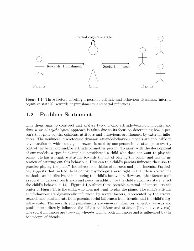
Figure 1.1: Three factors affecting a person’s attitude and behaviour dynamics: internalcognitive state(s), rewards or punishments, and social influences.

1.2 Problem Statement

This thesis aims to construct and analyse two dynamic attitude-behaviour models, andthus, a social psychological approach is taken due to its focus on determining how a per-son’s thoughts, beliefs, opinions, attitudes and behaviours are changed by external influ-ences. The nonlinear, discrete-time dynamic attitude-behaviour models are applicable inany situation in which a tangible reward is used by one person in an attempt to overtlycontrol the behaviour and/or attitude of another person. To assist with the developmentof our models, a specific example is considered: a child who does not want to play thepiano. He has a negative attitude towards the act of playing the piano, and has no in-tention of carrying out this behaviour. How can this child’s parents influence their son topractice playing the piano? Intuitively, one thinks of rewards and punishments. Psychol-ogy suggests that, indeed, behaviourist psychologists were right in that these controllingmethods can be effective at influencing the child’s behaviour. However, other factors suchas social influences from friends and peers, in addition to the child’s cognitive state, affectthe child’s behaviour [14]. Figure 1.1 outlines these possible external influences. At thecenter of Figure 1.1 is the child, who does not want to play the piano. The child’s attitudeand behaviour are dynamically influenced by several factors, represented by the arrows:rewards and punishments from parents, social influences from friends, and the child’s cog-nitive state. The rewards and punishments are one-way influences, whereby rewards andpunishments directly influence the child’s behaviour and attitude (but not vice versa).The social influences are two-way, whereby a child both influences and is influenced by thebehaviours of friends.

3


Child

Rewards

Parents

Figure 1.2: Conceptual representation of the one-person system.

This thesis considers two systems derived from Figure 1.1. Both models assume theparents offer their child a reward in an attempt to explicitly control him. The first assumesthe child does not experience social influences. Other important psychological assumptionsare also made but are discussed when the relevant concepts are introduced in future chap-ters. The first system can be considered within the typical plant-controller framework ofcontrol theory. The “plant” is a dynamic attitude-behaviour model of the child and the“controller” is the parents. Apart from the child’s initial attitude and behaviour, whichare negative, all of the plant’s initial conditions are zero. Furthermore, since the parentsinfluence their child through a sequence of rewards, the “control signal” is the reward.Finally, the child’s behaviour is the “system output”. Given that the plant contains thedynamics of one person, this system, conceptually shown in Figure 1.2, is referred to asthe one-person system.

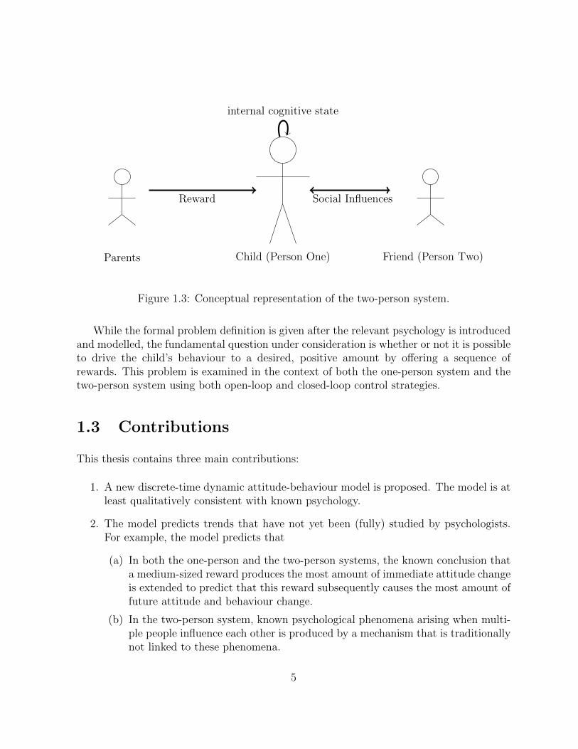
The conceptual representation of the second system, referred to as the two-person sys-tem, is shown Figure 1.3. This system drops the assumption that the child does notexperience social influences. Instead, the child is influenced by the behaviour of a friendand likewise, the friend is influenced by the behaviour of the child. Therefore, the two-person system plant contains dynamic attitude-behaviour models of both the child, thefriend and the effect these models have on each other. With the exception of each person’sinitial attitude and behaviour, all initial conditions are assumed to be zero. The initialattitude and behaviour of the child are negative and the initial attitude and behaviour ofthe friend are arbitrary. Similar to the one-person system, the control signal is the rewardoffered to the child (the friend is not offered a reward). Finally, the system output is thechild’s behaviour.

4


Child (Person One)

Reward

Parents

Social Influences

Friend (Person Two)

Figure 1.3: Conceptual representation of the two-person system.

While the formal problem definition is given after the relevant psychology is introducedand modelled, the fundamental question under consideration is whether or not it is possibleto drive the child’s behaviour to a desired, positive amount by offering a sequence ofrewards. This problem is examined in the context of both the one-person system and thetwo-person system using both open-loop and closed-loop control strategies.

1.3 Contributions

This thesis contains three main contributions:

1. A new discrete-time dynamic attitude-behaviour model is proposed. The model is atleast qualitatively consistent with known psychology.

2. The model predicts trends that have not yet been (fully) studied by psychologists.For example, the model predicts that

(a) In both the one-person and the two-person systems, the known conclusion thata medium-sized reward produces the most amount of immediate attitude changeis extended to predict that this reward subsequently causes the most amount offuture attitude and behaviour change.

(b) In the two-person system, known psychological phenomena arising when multi-ple people influence each other is produced by a mechanism that is traditionallynot linked to these phenomena.

5

3. Studying a dynamic attitude-behaviour model demonstrates the existence of inter-esting control problems in this new control systems application.

1.4 Thesis Overview

Following this introduction, the thesis continues with an overview of the relevant socialpsychological concepts associated with the one-person problem. Using these concepts, adiscrete-time, nonlinear model is developed and verified to be qualitatively consistent withthese concepts. In Chapter 3, the formal problem statement is given, followed by an in-vestigation of several open-loop and closed-loop control strategies. Chapter 4 extends theone-person plant to a two-person plant by introducing and applying social psychologicalconcepts describing how individuals influence each other; then model verification and con-trol strategies are discussed in Chapter 5. Finally, concluding remarks summarize the keyresults and highlight possible directions for future work.

6

Chapter 2

One-Person System:Psychology and Modelling

The thesis begins by exploring the one-person system: a child who does not want to play thepiano. The child’s parents wish to use a reward to influence their child to practice playingthe piano. The problem at hand is whether or not there exists a sequence of rewardsthat will induce the child to play the piano. Before answering this question, a dynamicattitude-behaviour model of the child is developed from the relevant social psychology.

The key “signals” of the one-person system are the child’s attitudes and behaviour. Awell-known result of social psychology, the theory of planned behaviour, is used to modelhow the child’s attitudes affect his behaviour. The theory of planned behaviour is a populardescription of an intuitive conclusion of psychology research: attitudes influence behaviour.Social psychologists have found sufficient evidence to suggest the converse is also true:behaviour influences attitudes. Support for this less-intuitive result is found in cognitivedissonance theory and the overjustification effect. Clearly, these two conclusions suggestthe attitude-behaviour relationship is dynamic. Indeed, psychology literature supportsthis suggestion [11]. Attitudes influence behaviours and vice versa; hence, from a controlsystems engineering perspective, the attitude-behaviour relationship forms a feedback loop.The feedback system block diagram is shown later (see Figure 2.3) after the necessarypsychology and signals have been defined.

Sections 2.1 and 2.2 present the relevant psychology theories, which are used in Sec-tion 2.3 to develop our model. The end of Section 2.3 includes an interpretation of thesignals in our model. After the model of the one-person system is developed, it is verifiedto be qualitatively consistent with the relevant psychology.

7

2.1 Psychology Describing How Attitudes

Drive Behaviour

The first step to understanding the attitude-behaviour relationship is studying how atti-tudes combine to form a behaviour. In this section, justification is given to explain thepsychological theory chosen for this component of our model. Following this justification,the theory is explained.

2.1.1 Background

Most people find it intuitive that actions follow attitudes, i.e., an individual’s internalbeliefs, thoughts, opinions and values will combine in some way to form his/her behaviour.However, this seemingly obvious result faced severe criticism in the 1970s, when manyexperimental studies suggested that behaviours do not necessarily follow attitudes. Thesecriticisms sparked a flurry of research on determining when attitudes predict behaviour.In [14], researchers conclude that attitudes predict behaviour when

(i) external influences are minimized,

(ii) attitudes are specific to the behaviour under consideration, and

(iii) the individual considers the attitudes as being important.

Researchers such as Icek Ajzen and Martin Fishbein extended these results by devel-oping models that incorporate the effect external influences have on behaviour formation.Indeed, their theory of planned behaviour considers several external factors affecting be-haviour, including rewards and social influences [11]. Not only is this theory well estab-lished in the psychology literature, it has a wide application range and is simple enoughfor modelling purposes. For these reasons, the theory of planned behaviour is chosen todescribe the influence attitudes have on behaviour.

2.1.2 Theory of Planned Behaviour

Icek Ajzen’s theory of planned behaviour [2], [11] stems from his earlier work with MartinFishbein: the theory of reasoned action [3]. Ajzen’s theory has been verified through manyexperimental results and thus, is well established in the psychology literature. The theoryof planned behaviour is a model of how people make reasoned decisions about performingor not performing a behaviour, based on various attitudes. For our model, attitudes are

8

not affected by irrational influences on attitude, such as emotion and motivation (but couldbe considered in future work).

The theory of planned behaviour is composed of five elements: behaviour, intent tobehave, attitude towards the behavioural outcome, external influences and perceived be-havioural control. These five elements are described in detail below:

1. Behaviour: The behaviour is some action that an individual may or may not perform.For the piano example, the behaviour the child is considering is “I will accept thereward from my parents and practise the piano today.” For our model, this decisionis made at each sample k, measured in days.

2. Intent to behave: Before a behaviour can be realized, there must be some intention toperform the behaviour. Essentially, the intent to behave is the individual’s assessmentof the likelihood that he/she will engage in a behaviour. Statements such as “Iwill try to execute behaviour x,” “I plan to execute behaviour x,” and “I expectI will execute behaviour x” represent the intent to execute behaviour x [11]. Anindividual’s behavioural intent may or may not yield the behaviour, but is a goodindicator that the behaviour will be performed. An intent to behave may not leadto the behaviour due to unforeseen circumstances that could make the behaviourimpossible. For example, suppose the child intends to accept the reward offered tohim by his parents and practise the piano. If, after this intention has been formed,the child realizes the piano has been stolen, then the child is not able play the piano.Since, however, intention is a good predictor of behaviour, the following assumptionis made:

Assumption 2.1. Behaviour and intent to behave are equal.

For this thesis, the terms behaviour, behavioural intent and intent to behave are usedinterchangeably and are denoted B[k]. An intent to perform the behaviour occurswhen B[k] ≥ 0 and an intent to not perform the behaviour occurs when B[k] < 0.Furthermore, the strength of this intention is represented by the magnitude |B[k]|.The notion of a positive behaviour and negative behaviours depends on the behaviouritself. For most behaviours, B[k] ≥ 0 is demonstrated by carrying out the behaviour,while the behaviour strength is an indicator of how much time and/or effort is putinto carrying out the behaviour. On the other hand, B[k] < 0 may not make sensefor particular behaviours (as could be the case for the piano situation). However, forsimplicity, we allow for negative behaviours. Investigating this issue in more detail isan item for future work. Finally, in practice there are various ways to measure B[k]and the attitude elements (Aout[k], Arew[k], described below), for example a 5-pointLikert scale [11]; thus, it is possible to quantify these values. For our model, we begin

9

with continuous values for B[k]. Considering discrete values for B[k] is an item offuture work.

3. Attitude towards the behavioural outcome: This element is the first of three contrib-utors to behavioural intent and is related to how a person feels about performing thebehaviour. Performing a behaviour results in one or more outcomes. Examples ofbehavioural outcomes of a child playing the piano may include: 1) feeling a sense ofaccomplishment; 2) becoming a more well-rounded person; and 3) becoming a socialoutcast. To keep our model simple, the following assumption is made:

Assumption 2.2. There is exactly one behavioural outcome.

Thus, suppose the child is concerned about only the first of the three aforementionedbehavioural outcomes. At each sample k, the child forms an attitude towards thisbehavioural outcome, denoted Aout[k]. Following a popular approach to attitudemodelling, the attitude consists of two factors: the likelihood the outcome will occur(the expectancy, E) and the importance the child places on the outcome (the value,V ). Both the expectancy and the value range from positive to negative values. Forexample, if the child believes that it is highly likely that playing the piano leads toa sense of accomplishment, then E > 0. On the other hand, if the child’s believesthat playing the piano is unlikely to lead to a sense of accomplishment, then E < 0.Finally, if the child believes that it is neither likely nor unlikely that playing thepiano leads to a sense of accomplishment, then E ≈ 0. Moreover, if feeling a sense ofaccomplishment is very important to the child, then V > 0, whereas V < 0 if the childfeels that it is entirely unimportant that he feels accomplished. Finally, V ≈ 0 whena sense of accomplishment is neither important nor unimportant to the child. Theinternal attitude, Aout, is formed from the product EV , i.e., Aout = EV ; thus fromTable 2.1, a positive internal attitude could have two interpretations (likewise for anegative attitude). For simplicity, assume the child values a sense of accomplishment,i.e., V > 0. If, at sample k, the child believes that practising the piano certainly leadsto a sense of accomplishment, then he has a high, positive attitude towards playingthe piano (i.e., Aout[k] � 0). On the other hand, if, at sample k, the child feels thebehavioural outcome is extremely unlikely, then his attitude towards the behaviouraloutcome is negative (i.e., Aout[k] � 0). Furthermore, Aout[k] is more moderate forless extreme beliefs about the likelihood that performing the behaviour leads to theoutcome in question. Finally, for simplicity, the terms attitude and internal attitudeare used interchangeably when referring to Aout[k].

4. External influences: This element is the second of three contributors to behaviouralintent and is related to a key result of psychology research: external influences aris-ing from rewards and other people affect an individual’s behaviour. Although this

10

E V Aout

negative negative positivepositive negative negativenegative positive negativepositive positive positive

Table 2.1: Attitude formation using the expectancy-value model. A negative expectancy(E) means the behavioural outcome is highly unlikely, whereas a positive expectancy meansthe behavioural outcome is highly likely. A negative value (V ) means the behaviouraloutcome is regarded as being totally unimportant, whereas a positive value means thebehavioural outcome is regarded as being very important.

result appears obvious, most people underestimate the extent to which these externalinfluences affect their behaviour, a phenomena termed by psychologists as the fun-damental attribution error [14]. For the one-person system, one external influence isconsidered: the effect of a reward on the individual’s behaviour. (For the two-personsystem, other external influences are also considered, as discussed in Section 4.1.)For our model, a monetary reward is used, where R[k] denotes the number of dollarsoffered to the child, at time k, to entice him to play the piano. Furthermore, theextent to which the child values money, denoted µ1, also contributes to the effect thereward has on the behavioural intent. This effect, is denoted Arew[k] and is referredto as the attitude towards the reward or reward attitude. Note that reward values arenon-negative and thus R[k] ≥ 0.

5. Perceived behavioural control: This element is the third of three contributors to be-havioural intent and is related to the extent to which a person believes the behaviourcan be executed. Two factors contribute to the perceived behavioural control: doubtsa person may have regarding his/her ability to perform the behaviour and known ob-stacles that may prevent the behaviour. For example, the child may doubt his abilityto play the piano if he hurt his hand, and thus, may have a lower behavioural intent.On the other hand, the child may recognize an actual obstacle, the absence of a pianofor example, and thus have a lower behavioural intent. For simplicity, the followingassumption is made:

Assumption 2.3. No doubts or obstacles arise that would reduce the behaviouralintent.

The theory of planned behaviour, conceptually shown in Figure 2.1, states that internalattitudes, external influences and perceived behavioural control together contribute to theformation of an intent to behave. Experimental results have shown that stronger internal

11

InternalAttitudes

ExternalInfluences

PerceivedBehavioural

Control

Behaviour

Aout[k]

Arew[k]

Figure 2.1: Conceptual representation of Ajzen’s theory of planned behaviour [2].

attitudes and external influences contribute to stronger intentions, whereas perceived be-havioural control has a “moderating” effect (i.e., a strong perceived behavioural controldoes not necessarily mean that a person will engage in the behaviour but a lower perceivedbehavioural control means a person is less likely to engage in the behaviour). Furthermore,the amount of weight placed on internal attitudes and external pressures affects the be-havioural intent. For example, when a large reward is offered to a child who values money,i.e., Arew[k] � 0, and who also has a large negative internal attitude, i.e., Aout[k] � 0,the behavioural intent that is formed may or may not be positive. If the internal attitudecarries more weight than the reward attitude, then the behavioural intent will be negative.Likewise, if the reward attitude carries more weight than the internal attitude, then thebehavioural intent will be positive. This weighting of attitudes and external pressures isknown to vary by individual and situation. Thus, for our model, this weighting is includedin the parameter values (see Table 2.2 for a summary of key parameters and signals thatappear in our model).

2.2 Psychology Describing How Behaviour

Drives Attitudes

The second step to understanding the attitude-behaviour relationship is studying ways inwhich behaviour can influence and change attitudes. These influences are characterized in

12

our model’s second component, thus closing the attitude-behaviour feedback loop. Severalwell-known, experimentally verified, psychological results support the seemingly counter-intuitive effect that behaviours influence attitudes, including cognitive dissonance theorydeveloped by Festinger [9], and the overjustification effect, proposed by Deci [7]. Thesetwo theories are selected to form the basis of our model’s “behaviour-driving-attitude”component. Cognitive dissonance theory is selected due to its wide application range andthe overjustification effect is used due to its relevance to how the one-person system iscontrolled: rewards.

2.2.1 Cognitive Dissonance Theory:Overview

Cognitive dissonance theory is one of social psychology’s most widely known and estab-lished theories. First proposed by Leon Festinger in 1957, cognitive dissonance has beenexperimentally verified in thousands of studies across dozens of settings, thus resulting inmany different paradigms [4], [9]. Among other things, the theory contains a non-intuitiveresult: behaviour can influence attitudes. Before discussing cognitive dissonance theory inthe context of our model and the piano example, a general understanding of the theory’sconcepts is required. Cognitive dissonance theory has two important concepts: dissonancepressure and dissonance pressure reduction.

Dissonance pressure is an uncomfortable psychological feeling that arises when a personholds two opposing cognitions (where a cognition is defined as knowledge of a thought,feeling, attitude or behaviour). For example, suppose a person who smokes cigaretteson a daily basis knows the harmful side-effects of his behaviour but has several friendswho also smoke. Since this person’s behaviour (choosing to smoke) is inconsistent withhis knowledge that smoking his bad for his health, he experiences dissonance pressure.However, the knowledge that he has several friends who also smoke is consistent with hissmoking behaviour. The smoker compares his behaviour cognition (termed the generativecognition by Beauvois and Joules [4]) with each of his other cognitions related to the actof smoking, thus forming cognitive pairs. If the behaviour cognition follows naturally fromthe other element in the cognitive pair, then the cognitive pair is said to be consistent. Onthe other hand, an inconsistent cognitive pair is one in which the two cognitions contradicteach other. Inconsistent cognitive pairs lead to dissonance pressure.

The extent to which a cognitive pair is consistent (or inconsistent) is given a magni-tude, denoted Mcon (or Mincon). The consistency (or inconsistency) magnitude indicateshow strongly the cognitive pair is consistent (or inconsistent). Festinger argues that themore strongly a cognition is held, the greater will be the consistency (or inconsistency)magnitude. The exact details of this calculations are given in Section 2.3.2. At this time,

13

it is only important to understand that each cognitive pair has an associated consistency orinconsistency magnitude (whatever the case may be) that is proportional to the strengthof each element in the cognitive pair.

Since dissonance pressure occurs when an inconsistent cognitive pair exists and such apair has an associated magnitude, it follows that dissonance pressure also has a magnitude,i.e., a person can experience different amounts of dissonance pressure. Indeed, Festingerprovides a description of dissonance pressure magnitude (P ) which Beauvois and Jouletransform into the following mathematical equation:

P =

∑Mincon∑

Mincon +∑Mcon

. (2.1)

Since, Festinger argues, dissonance pressure is an uncomfortable feeling, people want toreduce or eliminate it. This motivates the second concept of cognitive dissonance theory:dissonance pressure reduction. Festinger suggests three dissonance reduction techniques,outlined below:

(i) Decreasing (or eliminating) the inconsistency magnitude sum,∑Mincon. For the

smoking example, the smoker could, for instance, decrease the inconsistency magni-tude by believing that smoking is not as harmful as he once thought.

(ii) Increasing the consistency magnitude sum,∑Mcon. For the smoking example, the

smoker could accomplish this by changing the strength of the consistent cognition,i.e., he could believe a greater proportion of his friends smoke, or he could acquirenew smoking friends to increase the fraction who smoke.

(iii) Introducing a new, consistent cognition, thus increasing∑Mcon. For the smoking

example, the smoker could, for instance, begin to convince himself that smoking hasmore, and stronger, benefits (stress reduction, weight loss, etc.) than it really does.

These three techniques are consistent with how the magnitude given in (2.1) could bedecreased. Finally, the more dissonance pressure a person experiences, the more the personwill tend to perform these three dissonance reduction techniques.

2.2.2 Cognitive Dissonance Theory:Induced Compliance Paradigm

Cognitive dissonance theory is now discussed within the context of our model and thepiano example. The setup of the one-person problem, given in Chapter 1, indicates that

14

the child initially has a negative attitude and behaviour, i.e., Aout[0] < 0 and B[0] < 0.The child’s parents offer him a reward at some time k ≥ 0, thus producing a positivereward attitude, Arew[k] for k > 0. Thus, two cognitive pairs are formed: (Aout[k], B[k])and (Arew[k], B[k]). This setup follows the classic induced compliance paradigm of cogni-tive dissonance theory. In the induced compliance paradigm, a person is offered a rewardto do something he/she does not want to do. Moreover, the person does not experienceany other external influences. Classic induced compliance studies have shown that subjectsexperience dissonance pressure because one of their two cognitive pairs is inconsistent. Fur-thermore, in these studies, subjects were shown to reduce dissonance pressure by changingtheir internal attitude [10]. Thus, for our purposes, the following assumption is made:

Assumption 2.4. Dissonance pressure reduction occurs through change in Aout[k].

Note, for future work, our model could be extended to allow for other dissonancereduction methods.

The induced compliance paradigm considers two different cases, one in which the re-ward is large enough to induce a positive behaviour and the one in which the reward isinsufficient. In each of these cases, dissonance pressure arises. First, the factors contribut-ing to dissonance pressure are discussed, followed by an investigation into the relationshipbetween how the amount of dissonance pressure varies with respect to the reward value.Then, for the two cases, dissonance pressure reduction methods are presented. Let Case Abe the situation in which a sufficiently large reward is offered, thus inducing a positivebehaviour. Let Case B be the situation in which the reward is insufficient at producing apositive behaviour.

In Case A, the sufficiently large reward produces a positive behaviour and therefore,the reward attitude and the behaviour are consistent. On the other hand, the positive be-haviour and the negative internal attitude are inconsistent and hence, dissonance pressurearises. When a person is given a reward that is just large enough to produce a positivebehaviour, some amount of dissonance pressure occurs. If, instead, a larger reward is of-fered, then less dissonance pressure occurs because the person essentially rationalizes theirbehaviour as being due to the reward (instead of their internal attitude). Therefore, inCase A, larger rewards produce less dissonance pressure.

In Case B, the reward is insufficient and thus, produces a negative behaviour, whichforms an inconsistency between the reward attitude and the behaviour. Due to this incon-sistency, dissonance pressure arises. Note, however, that in this case, the negative internalattitude is consistent with the negative behavioural intent. Like Case A, the amount ofdissonance pressure a person experiences varies with respect to the reward value. When aperson is offered a very small reward, a small amount of dissonance pressure occurs becausehe/she is rejecting a small reward. However, the dissonance pressure is larger in the case

15

reward

dissonance pressure magnitude

R∗

Case B Case A

Figure 2.2: Short-term relationship between dissonance pressure magnitude and amountof reward when initial attitude is negative [9]. R∗ is the smallest reward value that issufficiently large to induce a positive behaviour. As the reward value varies from zero toR∗, dissonance pressure increases. As the reward value varies from R∗ to infinity, dissonancepressure decreases. This figure looks only at the short-term relationship between dissonancepressure magnitude and reward, as the dissonance pressure magnitude can change overtime.

of larger (but still insufficient) rewards. This increased dissonance pressure is due to theperson rejecting a larger reward, which is a more uncomfortable experience. Therefore, inCase B, larger rewards produce more dissonance pressure.

In Figure 2.2, the relationship describing how dissonance pressure varies with respectto the reward is shown in graphical form. In this thesis, this relationship is termed thedissonance triangle. Festinger notes that the dissonance triangle does not represent theexact mathematical equation for calculating dissonance pressure. Instead, Festinger arguesthat the exact nature of the relationship has yet to be determined. As will be shown inChapter 3, our model is consistent with Figure 2.2.

Now, dissonance pressure reduction is considered for the two situations. In Case A,the internal attitude is negative and the behaviour is positive, i.e., for some sample k,Aout[k] < 0 and B[k] ≥ 0. Clearly, (Aout[k], B[k]) form the inconsistent cognitive pair. ByAssumption 2.4, dissonance pressure is reduced by increasing or decreasing Aout[k]. SinceAout[k] contributes to the inconsistency magnitude and from before, dissonance pressurecan be reduced by decreasing

∑Mincon, the inconsistency magnitude must decrease. There

are two ways to achieve this:

1. The internal attitude can become less negative (but still remain negative); thus,

16

reducing the strength of Aout[k] and consequently,∑Mincon.

2. The internal attitude can become positive; thus, eliminating∑Mincon and introduc-

ing a new, consistent cognition, which increases∑Mcon. In this situation, two of the

three techniques outlined in Section 2.2.1 are employed simultaneously.

In both cases, Aout[k] basically increases to reduce dissonance pressure.

On the other hand, in Case B, the behaviour is negative and therefore, (Aout[k], B[k])form the consistent cognitive pair. By Assumption 2.4, dissonance is reduced by increasingor decreasing Aout[k]. Since Aout[k] contributes to the consistency magnitude and frombefore, dissonance pressure can be reduced by increasing

∑Mcon, the consistency magni-

tude must increase. For our model, this increase can only occur by the internal attitudebecoming more negative; hence, for Case B, Aout[k] decreases to reduce dissonance pressure.

To summarize, in the induced compliance paradigm, dissonance pressure arises when areward is offered to induce a “counter-attitudinal” behaviour. The amount of dissonancepressure varies with respect to the reward value, as shown in Figure 2.2. When the rewardis sufficiently large, dissonance pressure reduces through the internal attitude becomingless negative, i.e., Aout[k] increases; whereas in the case of an insufficient reward, disso-nance pressure reduces through the internal attitude becoming more negative, i.e., Aout[k]decreases.

2.2.3 The Overjustification Effect

Cognitive dissonance theory suggests how behaviour can affect attitudes when there areinconsistent cognitions. If all attitudes are consistent with behaviour, then cognitive disso-nance theory concludes no dissonance pressure arises and thus predicts no attitude changeoccurs. However, researchers including Edward Deci and colleagues have shown that atti-tude can still change when all cognitions are consistent [8]. Specifically, when a person hasa positive internal attitude towards a behaviour and is offered a reward in a controllingmanner, then the person’s internal attitude will decrease. Hence, it is counter-productive tooffer a person a reward if his attitude is already positive. This is called the overjustificationeffect.

The overjustification effect can be explained through attribution theory : the personattributes their performance of the behaviour to the reward instead of their internal atti-tude, i.e., the person thinks “I must be performing the behaviour because I’m getting areward and therefore, I am less motivated to perform this behaviour without a reward.” Ina study on the overjustification effect, [7], subjects who were were interested in an activitywere given a reward to continue performing the activity. Upon removal of the reward, thesubjects still continued the activity, but to a much lesser extent. Thus, from the theory of

17

planned behaviour, the internal attitude must have decreased to account for the differencebetween pre-reward and post-reward behaviour strength. Important to note is the fact thateven though the internal attitude decreases, it does not stop the behaviour altogether, thus,the attitude does not become negative. Furthermore, the initial strength of the attitudeand the reward amount were both factors in the amount of attitude change.

The dynamic attitude-behaviour model proposed in this thesis includes the overjusti-fication effect due to the possibility in the induced compliance paradigm that the child’sinternal attitude may become positive (see Case A of the induced compliance paradigm inSection 2.2.2). In this case, the child’s behaviour, internal attitude and reward attitudeare all positive, so overjustification pressure arises, causing attitude to decrease.

2.3 A Dynamic Attitude-Behaviour Model

The three social psychological theories introduced in Sections 2.1 and 2.2 are now com-bined to form a discrete-time dynamic attitude-behaviour model. Even though it seemsnatural to consider human attitude and behaviour as a varying continuously with time, adiscrete-time model is developed for two reasons. First, attitude measurement cannot bedone instantaneously. However, the area of research pertaining to attitude measurement,psychometrics, provides methods to sample an individual’s attitude. Thus, it is natural tofollow this discrete-time approach. Second, a continuous-time reward signal makes littlesense from a practical perspective. When a reward is offered, it is offered at a certain pointin time and thus, the system input is a discrete-time signal.

The second modelling decision that has been made involves how dynamics are incor-porated into our model. Two factors contribute to the system’s dynamics: feedback andmental processing. The first factor, as previously discussed, incorporates feedback intothe attitude-behaviour model to account for the feedback nature of the attitude-behaviourrelationship. The second factor accounts for the mental processing that occurs when anew attitude is formed or pressure is experienced. Researchers in the field of cognitivepsychology have concluded that humans take time to mentally process information; thus,following standard research on mental processing dynamics [17], first-order lag mental pro-cessing dynamics are assumed throughout our model.

Figure 2.3 provides a high-level diagram of our model. Component A essentially modelsthe theory of planned behaviour, while Component B models how cognitive dissonancetheory and the overjustification effect result in changes to Aout. The overall change, asindicated in the figure, is denoted ∆Aout[k]. Component A and Component B are examinedmore carefully below. See Table 2.2 for a summary of key parameters and signals.

18

Sym

bol

Desc

ripti

on

[valueorunits]

Aout[k]∈

(−∞,∞

)at

titu

de

tow

ards

the

beh

avio

ur

outc

ome

[att

itu

deu

nit

s]∆Aout[k]∈

(−∞,∞

)ch

ange

inat

titu

de

tow

ards

the

beh

avio

ur

due

toco

gnit

ive

dis

so-

nan

cean

dov

erju

stifi

cati

oneff

ects

[att

itu

deu

nit

s]Arew

[k]∈

[0,∞

)at

titu

de

tow

ards

acce

pti

ng

are

war

dto

per

form

the

beh

avio

ur

[at-

titu

deu

nit

s]R

[k]∈

[0,∞

)re

war

dva

lue

[dol

lars

]B

[k]∈

(−∞,∞

)b

ehav

iour

[att

itu

deu

nit

s]PCD

raw

[k],PCD

[k]∈

(−0.

5,0.

5)pre

ssure

aris

ing

from

cogn

itiv

edis

sonan

ceeff

ects

[un

itle

ss]

POJ

raw

[k],POJ[k

]∈

[0,∞

)pre

ssure

aris

ing

from

the

over

just

ifica

tion

effec

t[(

atti

tude

un

its)

2]

K1∈

[0,∞

)†ga

inre

flec

ting

how

the

dis

sonan

cepre

ssure

affec

tsat

titu

de

chan

ge[K

1=

30at

titu

deu

nit

s]K

2∈

[0,∞

)†ga

inre

flec

ting

how

the

over

just

ifica

tion

pre

ssure

affec

tsat

titu

de

chan

ge[K

2=

0.1

1/(a

ttit

ude

un

it)]

µ1∈

(0,∞

)va

lue

assi

gned

toon

edol

lar

[1at

titu

deu

nit

per

doll

ar]

r 1∈

[0,1

)†m

enta

lpro

cess

ing

pol

elo

cati

onfo

rre

war

dat

titu

de

form

atio

nin

(2.3

)[r

1=

0]r 2∈

[0,1

)†m

enta

lpro

cess

ing

pol

elo

cati

onfo

rdis

sonan

cepre

ssure

in(2

.11)

[r2

=0.

5]r 3∈

[0,1

)†m

enta

lpro

cess

ing

pol

elo

cati

onfo

rov

erju

stifi

cati

oneff

ect

in(2

.14)

[r3

=0.

5]

Tab

le2.

2:K

eysi

gnal

san

dpar

amet

ers

that

app

ear

inth

em

odel

.T

he

par

amet

erva

lues

list

edar

eth

ose

use

dfo

ran

alysi

sin

Chap

ter

3.P

aram

eter

sm

arke

d†

dep

end

onsa

mpling

per

iod,

take

nher

eto

be

one

day

.

19

Component B

Cognitive DissonanceOverjustification

Component A

Theory of Planned Behaviour

R[k]

Arew[k]

Aout[k]

B[k] B[k]

Aout[k]

∆Aout[k]

Figure 2.3: Block diagram of the one-person system (dotted box), decomposed into Com-ponents A and B. The system input is R[k], and the system outputs are Aout[k] and B[k].

2.3.1 Details of Component A

Component A is based on the theory of planned behaviour, discussed in Section 2.1.2,which states that an individual’s behaviour is formed from his/her internal attitude andexternal influences (assuming full perceived behavioural control). The internal attitudedepends on how much attitude change is formed through dissonance and overjustificationpressures. The reward attitude depends on the reward in dollars (R[k]), how much thereward is valued (µ1), and a first-order mental processing model (with r1 denoting the polelocation). From the theory of planned behaviour, stronger internal attitudes and externalinfluences cause stronger behavioural intent. Moreover, a weighting factor influences theextent to which each of these elements affects B[k]. For our model, this weighting iscontained in µ1. Thus, Component A is modelled by the following three equations:

Aout[k] = Aout[k − 1] + ∆Aout[k − 1] (2.2)

Arew[k] = r1Arew[k − 1] + µ1 (1− r1)R[k − 1] (2.3)

B[k] = Aout[k] + Arew[k]. (2.4)

2.3.2 Details of Component B

Component B, shown in more detail in Figure 2.4, is based on cognitive dissonance theoryand the overjustification effect. These two psychological effects create pressure, producingattitude change. Thus, the output of Component B is ∆Aout[k], the change in attitude

20

∆Aout[k]

(2.15) (2.14) (2.13)

(2.12) (2.11) (2.10)

B[k]Aout[k]Arew[k]

∆ACDout [k] PCD[k] PCD

raw[k]

∆AOJout[k] POJ [k] POJ

raw[k]

Figure 2.4: Details of Component B. The thick line is used to indicate multiple signals.

towards the behavioural outcome:

∆Aout[k] = ∆ACDout [k] + ∆AOJout[k]. (2.5)

Each of the terms in (2.5) will now be examined.

Cognitive Dissonance Theory Model

As discussed in Section 2.2.2, the effects due to the induced compliance paradigm of cog-nitive dissonance theory arise when Aout[k] < 0 and Arew[k] > 0. If these two inequalitieshold, then each of these cognitions form a cognitive pair with the generative cognition,B[k], one of which is inconsistent, thus causing dissonance pressure and attitude change.

The dissonance pressure magnitude equation in (2.1) depends on∑Mcon and

∑Mincon.

For the one-person system, there are two cognitive pairs, (Aout[k], B[k]) and (Arew[k], B[k]),each of which have an associated Mcon[k] and Mincon[k]. Festinger states that these mag-nitudes are proportional to the strength of each element in the cognitive pair; thus, define

M1incon[k] =

{|Arew[k]B[k]| if Arew[k] > 0, B[k] < 0,

0 otherwise,(2.6)

M2incon[k] =

{|Aout[k]B[k]| if Aout[k] < 0, B[k] > 0,

0 otherwise,(2.7)

21

and

M1con[k] =

{|Arew[k]B[k]| if Arew[k] > 0, B[k] > 0,

0 otherwise,(2.8)

M2con[k] =

{|Aout[k]B[k]| if Aout[k] < 0, B[k] < 0,

0 otherwise.(2.9)

Let Mincon[k] =∑2

i=1Miincon[k] and Mcon[k] =

∑2i=1 M

icon[k]. Then, the (raw, unprocessed)

dissonance pressure at time k is:

PCDraw [k] =

sgn (B[k]) Mincon[k]

Mincon[k]+Mcon[k]if Aout[k] < 0, Arew[k] > 0, and B[k] 6= 0,

|Aout[k]||Aout[k]|+|Arew[k]| if Aout[k] < 0, Arew[k] > 0, and B[k] = 0,

0 otherwise.

(2.10)

The first case in (2.10) captures the cognitive dissonance effects in all situations exceptthe special situation B[k] = 0, where a division by zero error would occur. The specialsituation B[k] = 0 is handled in the second case in (2.10). The “sgn (B[k])” factor ensuresthat the sign of ∆ACDout [k] is consistent with cognitive dissonance theory in that it resultsin a decrease in dissonance pressure at the next time instant.

Having derived an expression for the raw dissonance pressure, the first-order mentalprocessing model is applied as follows. Let PCD[k] represent the actual dissonance pressureexperienced at time k. Then,

PCD[k] = r2PCD[k − 1] + (1− r2)PCD

raw [k]. (2.11)

Finally, the dissonance pressure results in attitude change, denoted ∆ACDout [k], given by

∆ACDout [k] = K1PCD[k]. (2.12)

In (2.12), it is assumed that attitude change is proportional to the dissonance pressure;psychologists have yet to identify the exact relationship.

The Overjustification Effect Model

As discussed in Section 2.2.3, the overjustification effect applies only when Arew[k] > 0,Aout[k] > 0 and B[k] > 0. The basic pressure arising from the overjustification effect ismodelled as

POJraw[k] =

{Aout[k]Arew[k] if Aout[k] > 0, B[k] > 0, and Arew[k] > 0,

0 otherwise.(2.13)

22

In (2.13), it is assumed that the pressure depends on the product of the relevant attitudes.The use of a product is somewhat arbitrary; psychologists have not yet determined theexact relationship, so any function that increases in magnitude with each of Aout[k] andArew[k] would be equally justified.

Assuming first-order mental processing of the pressure POJraw[k], the following equation

for the processed pressure is obtained:

POJ [k] = r3POJ [k − 1] + (1− r3)POJ

raw[k]. (2.14)

Finally, to avoid the situation where POJ [k] is large enough to actually change the sign ofAout[k] (an effect that is inconsistent with overjustification theory), POJ [k] is saturated asfollows:

∆AOJout[k] =

−K2P

OJ [k] if POJ [k] > 0, K2POJ [k] ≤ Aout[k],

−Aout[k] if POJ [k] > 0, K2POJ [k] > Aout[k],

0 otherwise.

(2.15)

As in (2.12), attitude change is assumed to be proportional to the experienced psychologicalpressure.

The terms ∆ACDout [k] and ∆AOJout[k] handle the basic one-person configuration. The two-person system, discussed in Chapter 4, contains additional equations modelling the effectanother significant person has on the attitude-behaviour model.

2.3.3 Simplifying Assumptions and Initial Conditions

Along with the problem statement given in Chapter 1, the psychology behind this discrete-time model suggests initial conditions. In particular, the child in the one-person systeminitially has a negative internal attitude. Furthermore, it can be reasonably assumedthat he has not previously been offered a reward; thus, initially, his behavioural intentmatches his negative attitude. A second reasonable assumption is that the child has notpreviously experienced any pressures due to dissonance or overjustification effects and thus,experiences no initial attitude change.

In the context of our model, these initial conditions are given by:

PCD[0] = POJ [0] = 0,

∆ACDout [0] = ∆AOJout[0] = 0,

Arew[0] = 0,

B[0] = Aout[0] = Ao, (2.16)

where Ao < 0.

Additionally, the following assumptions are made on the parameter values:

23

Assumption 2.5. Gains reflecting how the dissonance and overjustification pressures af-fect attitude change are strictly positive, i.e., K1 > 0 and K2 > 0.

Assumption 2.6. The value assigned to one dollar is strictly positive, i.e., µ1 > 0.

Assumption 2.7. The mental processing pole location for reward attitude formation in(2.3) is zero, i.e., r1 = 0.

Assumption 2.7 simplifies the expressions for Arew[k] in (2.3) to

Arew[k] = µ1R[k − 1]. (2.17)

Assumption 2.8. The mental processing pole locations for dissonance and overjustifi-cation pressures in (2.11) and (2.14) respectively, are contained in the range [0, 1), i.e.,0 ≤ r2, r3 < 1.

These assumptions are used throughout the remainder of this chapter, as well as in Chap-ter 3.

2.3.4 Interpreting the Discrete-Time Model

From a practical perspective, it is useful to understand how to interpret Aout[k], Arew[k],R[k], B[k] and ∆Aout[k]. Since a discrete-time approach is taken, it is natural to alsodiscuss the timing sequence of these signals, summarized in Table 2.3. This discussionconsiders the motivating piano situation with a sample period of one day, using the valuesin Table 2.2.

On the morning of the first day (k = 0), the child’s internal attitude towards playingthe piano is negative (say, Ao = −15 attitude units) and since he has not previously beenoffered a reward, his reward attitude is zero (say, Arew[0] = 0 attitude units). These twoattitudes combine to form the child’s intent to play the piano at some point during thefirst day (B[0] = −15 attitude units). Since the child does not intend to practise piano onday one, his parents offer him a reward at the end of the day (say, R[0] = $16) to inducetheir child to play piano on the next day. From (2.3), the child needs time to mentallyprocess this reward; thus it is clear this reward does not influence B[0].

On the morning of the second day (k = 1), the child’s attitude is the same (because nodissonance or overjustification pressures arose on the first day, i.e., ∆Aout[0] = 0). However,the child has had sufficient time to mentally process the reward offered by his parents onthe previous evening. This processed reward has formed an attitude towards the rewardthat was offered to play the piano at some point on day two (Arew[1] = 16 attitude units).In this example, the internal attitude and reward attitude combine to form a positive

24

Day 1 Day 2 Day 3(k = 0) (k = 1) (k = 2)

Aout[k] −15 −15 −12.58Arew[k] 0 16 16

B[k] −15 1 3.419∆Aout[k] 0 2.4194 3.4106

R[k] 16 16 16

Table 2.3: Timing chart portraying sequence of events at each time step. At the beginningof each day, the child wakes up with an internal attitude, Aout[k], and an attitude towardsaccepting a reward and playing the piano, Arew[k]. These two attitudes form a behaviouralintent, B[k], which translates into the child engaging (or not engaging) in the behaviour tosome degree throughout the day. Once this behaviour is realized, the child may or may notexperience pressure (due to effects from dissonance and/or overjustification). This pres-sure creates an attitude change, which must undergo mental processing before influencingAout[k] (see (2.2)). At the end of the day, the parents offer their child some reward, R[k],to induce their child to practise the piano on the subsequent day.

behavioural intent, i.e., the child decides to accept the reward and practise piano on daytwo (B[1] = 1 attitude units). The amount of time and effort he spends practising thepiano is related to the strength of his behavioural intent, |B[k]|. At the end of the day, thechild has played the piano and thus, since B[1] > 0 and Aout[1] < 0, the child experiencesdissonance pressure. However, due to mental processing, this dissonance pressure does notaffect Aout[1]. Instead, the dissonance pressure causes the child to wake up on the morningof the third day with a new attitude (because Aout[2] = Aout[1]+∆Aout[1] and ∆Aout[1] > 0due to dissonance pressure). Finally, suppose the parents choose to offer their son the samereward on the evening of day two to induce him to play the piano on day three.

The same sequence of events occurs on the third day. However, where on the morningof day two the internal attitude remained the same, on the morning of day three, thechild wakes up with a changed attitude, due to the dissonance pressure experienced on theprevious day. From (2.12), the dissonance pressure experienced on day two produces someamount of attitude change. This attitude change undergoes mental-processing by the child(see (2.2)) and thus influences attitude such that on the beginning of day three, the childhas a new attitude. This sequence of events continues for each subsequent day.

25

2.4 Model Consistency Verification

Typically, after a system is modelled, model validation is performed. However, for ourmodel, the amount of time required for adequate validation is quite large. Additionally,further expertise and resources are needed to perform the psychology experiments necessaryfor formal model verification. Finally, it is unclear if experts in the field of psychometrics,which among other things, studies the measurement of attitudes and behaviours, are ableto reliably measure all of the key signals in our model, such as dissonance pressure. Forthese reasons, a model consistency verification is conducted instead of formal model vali-dation. For this verification, the consistency between the one-person system, developed inSection 2.3, and the relevant psychological theories, introduced in Sections 2.1 and 2.2, isstudied. This model consistency verification is accomplished by comparing key qualitativecharacteristics and trends of the relevant psychology theories (the theory of planned be-haviour, cognitive dissonance theory and the overjustification effect) with the qualitativecharacteristics and trends of signals within our model.

The theory of planned behaviour, which describes how attitudes combine to generatea behavioural intent, has two qualitative trends:

1. When all attitudes are positive (or negative), behavioural intent is positive (or neg-ative).

2. An increase (or decrease) in any one attitude causes an increase (or decrease) inbehavioural intent.

By inspection of the behavioural intent equation given in (2.4), it is clear that our modelis consistent with these two characteristics.

The induced compliance paradigm of cognitive dissonance theory suggests, among otherthings, how behaviour can influence attitude through dissonance pressure and exhibits twodistinct qualitative trends:

1. From general cognitive dissonance theory, people tend to reduce the dissonance pres-sure magnitude, should it arise.

2. From the induced compliance paradigm, the relationship between the reward andthe dissonance pressure magnitude is similar to the dissonance triangle, shown inFigure 2.2.

In addition to these two qualitative trends, Festinger proposed a quantitative feature ofcognitive dissonance theory. In [9], Festinger states “that the weighted proportion of[inconsistent cognitions] cannot be greater than 50 per cent.” This suggests a maximum

26

dissonance pressure of 50 per cent, or 0.5; hence, verification is performed to determinewhether or not our model is consistent with this conclusion. Now our model is shown toexhibit these three characteristics.

To verify if the one-person system exhibits the first trend, recall that by Assump-tion 2.4, dissonance reduction occurs through attitude change. Now, consider the mod-elling equations associated with cognitive dissonance pressure and the resulting attitudechange, i.e., (2.6)–(2.12). Verifying that dissonance pressure is reduced through attitudechange amounts to showing that when PCD

raw [k] 6= 0, following relationship holds:

|PCDraw [k + 1]| < |PCD

raw [k]|

when Aout[k + 1] 6= Aout[k]. The raw, unprocessed dissonance pressure is considered herebecause the mental processing dynamics make it more challenging to compare the amountof dissonance pressure arising at each sample. If the above relationship is shown to betrue, then, since the mental processing dynamics are simply modelled by a first-order lagtransfer function, the processed dissonance pressure magnitude also decreases eventually.Furthermore, the magnitude is considered because it represents the amount or strength ofthe dissonance pressure.

From (2.10), the internal attitude must be negative and the reward attitude must bepositive for raw, unprocessed dissonance pressure to arise. To understand why, considera non-negative internal attitude. This internal attitude, combined with a positive reward,generates a positive behaviour and therefore, both cognitive pairs are consistent, i.e., dis-sonance pressure does not arise. Suppose instead, that the internal attitude is negativebut the reward attitude is zero; then, the behavioural intent is the same at the internalattitude and again, both cognitive pairs are consistent. Therefore, in both the case whenAout[k] ≥ 0 and when Arew[k] = 0, the raw, unprocessed dissonance pressure is zero.

Supposing Aout[k] < 0 and Arew[k] > 0, two cases must be considered. These two casesmatch Case A and Case B from the induced compliance paradigm discussed in Section 2.2.2,i.e., the first case considers when B[k] ≥ 0 and the second case considers when B[k] <0. For the situation in which B[k] ≥ 0, from (2.6)–(2.9), Mincon[k] = |Aout[k]B[k]| andMcon[k] = |Arew[k]B[k]|. Assuming B[k] 6= 0, from (2.10),

PCDraw [k] =

|Aout[k]B[k]||Aout[k]B[k]|+ |Arew[k]B[k]|

=|Aout[k]|

|Aout[k]|+ |Arew[k]|. (2.18)

Note that if B[k] = 0, then PCDraw [k] = |Aout[k]|

|Aout[k]|+|Arew[k]| , which is the same as the above

expression. From (2.11), this raw, unprocessed dissonance pressure produces a positivePCD[k] and thus from (2.12) a positive attitude change, i.e.,

Aout[k + 1] = Aout[k] +K1PCD[k] > Aout[k].

27

Note that ∆AOJout[k] = 0 since the conditions required for overjustification effect to holdare not met. The above expression is consistent with Case A of the induced complianceparadigm. A sufficiently large reward that is able to produce a positive behavioural intenthas the effect of causing a negative attitude to increase. To see how this affects the raw,unprocessed dissonance pressure at sample k + 1, assume that this increased attitude,Aout[k + 1] is still negative (otherwise, PCD

raw [k + 1] = 0 and thus, dissonance pressure isreduced). Furthermore, since the reward attitude also contributes to the magnitude ofPCDraw [k], assume the reward attitude is constant to ensure only the effects of changes to the

internal attitude are studied. Since the internal attitude increases and the reward remainsconstant, B[k] necessarily increases and is therefore, still positive. Hence, from (2.10),

PCDraw [k + 1] =

|Aout[k + 1]B[k + 1]||Aout[k + 1]B[k + 1]|+ |Arew[k + 1]B[k + 1]|

=|Aout[k + 1]|

|Aout[k + 1]|+ |Arew[k + 1]|.

Since Arew[k + 1] = Arew[k] and |Aout[k + 1]| < |Aout[k]| (because Aout[k] < Aout[k + 1]and both are negative), it follows that PCD

raw [k + 1] < PCDraw [k] as required. Note that since

PCDraw [k] > 0, the magnitude signs are omitted.

For the situation in which B[k] < 0, from (2.6)–(2.9), Mcon[k] = |Aout[k]B[k]| andMincon[k] = |Arew[k]B[k]|. From (2.10),

PCDraw [k] = − |Arew[k]B[k]|

|Arew[k]B[k]|+ |Aout[k]B[k]|= − |Arew[k]||Arew[k]|+ |Aout[k]|

. (2.19)

From (2.11), this raw, unprocessed dissonance pressure produces a negative PCD[k] andthus from (2.12) a negative attitude change, i.e.,

Aout[k + 1] = Aout[k] +K1PCD[k] < Aout[k].

Similar to before, ∆AOJout[k] = 0. The above expression is consistent with Case B of theinduced compliance paradigm. An insufficient reward that is not able to produce a positivebehavioural intent has the effect of causing a negative attitude to decrease. This decreaseeffectively decreases B[k] (again, assuming a constant reward attitude). Hence, from (2.10),

PCDraw [k + 1] = − |Arew[k + 1]B[k + 1]|

|Arew[k + 1]B[k + 1]|+ |Aout[k + 1]B[k + 1]|

= − |Arew[k + 1]||Arew[k + 1]|+ |Aout[k + 1]|

.

Since Arew[k+ 1] = Arew[k] and |Aout[k+ 1]| > |Aout[k]| (because Aout[k] > Aout[k+ 1] andboth are negative), it follows that |PCD

raw [k + 1]| < |PCDraw [k]| as required.

28

For illustrative purposes, two simulations are performed, shown in Figure 2.5. In bothsimulations, a step reward is applied to the one-person system with the initial conditionsgiven in (2.16) and the parameter values given in Table 2.2. The first simulation, shown inthe left-hand side plots, is related to Case A of the induced compliance paradigm, whereasthe right-hand side plots are the results of the second simulation, related to Case B. Asboth simulations show, when dissonance pressure arises, the raw, unprocessed dissonancepressure decreases through attitude change. Furthermore, the processed dissonance pres-sure, PCD[k] also decreases, as expected. Therefore, our model is consistent with thefirst qualitative characteristic of the induced compliance paradigm of cognitive dissonancetheory.

Next, the second characteristic related to cognitive dissonance on page 26, which de-scribes the relationship between the reward and the dissonance pressure magnitude, isconsidered. Again, the unprocessed dissonance pressure is studied due to the additionalcomplexity arising from the mental processing dynamics. From Section 2.2.2, the rewardand the dissonance pressure magnitude should exhibit the dissonance triangle relationship,given in Figure 2.2. The dissonance triangle indicates that the larger of two insufficientrewards produces more dissonance pressure than the smaller of these two rewards, whereasthe larger of two sufficiently large rewards produces less dissonance pressure. To check ifour model is consistent with this conclusion, the expression for the raw, unprocessed dis-sonance pressure is examined. From before, there are two possible expression for PCD

raw [k]:(2.18) and (2.19). To determine how the magnitude of these two expressions varies withrespect to Arew[k], fix Aout[k] to some constant value. In Case A, when B[k] ≥ 0, PCD

raw [k]is given by (2.18). For some fixed Aout[k], increasing Arew[k] produces a smaller PCD

raw [k](since Arew[k] is only in the denominator term of the expression). Therefore, for sufficientlylarge rewards, greater rewards produce smaller dissonance pressure. On the other hand, inCase B, when B[k] < 0, PCD

raw [k] is given by (2.19). This expression can be rearranged to

|PCDraw [k]| = 1

1 + |Aout[k]|Arew[k]

.

Again, the magnitude is considered because the sign simply indicates the attitude changedirection. From the above expression it is evident that for a fixed Aout[k], larger valuesof Arew[k] produce larger values of |PCD

raw [k]|. Therefore, for insufficient rewards, greaterrewards produce greater dissonance pressure. The relationship between the reward attitudeand the dissonance pressure is illustrated in Figure 2.6. In the figure, the expressions forPCDraw [k] are plotted with respect to Arew[k]. For insufficient rewards, the expression given

in (2.19) is used, whereas (2.18) is used for sufficiently large rewards. Figure 2.6 clearlydemonstrates that our model exhibits the same dissonance triangle relationship predictedby Festinger.

In addition to the two qualitative trends of cognitive dissonance theory, the final charac-teristic, which is quantitative in nature, is considered by analysing the maximum dissonance

29

0 5 100

10

20

0 5 10

−60−40−20

0

0 5 100

0.5

0 5 10−60−40−20

020

sample (k)

0 5 100

10

20

0 5 10

−60−40−20

0

0 5 100

0.5

0 5 10−60−40−20

020

sample (k)

Arew[k]

R[k]

Aout[k]

Aout[k]

|PCDraw[k]| |PCD

raw[k]|

|PCD[k]|

B[k]

B[k]

Arew[k]R[k]

|PCD[k]|

Figure 2.5: Simulation demonstrating how the one-person system with the initial condi-tions given in (2.16) responds to a step reward. Set Ao = −15 attitude units and considertwo step reward magnitudes: a reward that is sufficiently large enough to produce posi-tive behavioural intent (R[k] = $20, left plots), and a reward that is not sufficiently large(R[k] = $10, right plots). For a sufficiently large reward, the magnitude of Aout[k] firstdecreases and, as a result, Aout[k] becomes less negative. This has the effect of reducingPCDraw [k] and PCD[k]. Note though, that once attitude becomes positive, overjustification

pressure arises and affects Aout[k]. For an insufficient reward, Aout[k] decreases, thus in-creasing its magnitude. This has the effect of reducing PCD

raw [k] and PCD[k]. B[k], R[k] andArew[k] are also included in the above plots.

30

0 5 10 15 20 25 30 35 40 45 500

0.05

0.1

0.15

0.2

0.25

0.3

0.35

0.4

0.45

0.5

Arew[k]

|PC

Dra

w[k

]|

Figure 2.6: Relationship between raw, unprocessed dissonance pressure magnitude andreward attitude for the one-person system. Set Aout[k] = −15 attitude units ; then,the raw, unprocessed dissonance pressure magnitude, |PCD

raw [k]|, is calculated using(2.19) when Arew[k] ∈ [0 attitude units, 15 attitude units) and (2.18) when Arew[k] ∈[15 attitude units, 50 attitude units]. The left-hand side of the plot is related to Case B,whereas the right-hand side of the plot is related to Case A.

31

pressure magnitude. Festinger’s proposition that the weighted amount of inconsistent cog-nitive pairs must be less than 50 per cent suggests that the raw, unprocessed dissonancepressure has a maximum value. The raw, unprocessed dissonance pressure, PCD

raw [k], is afraction; consequently, the maximum dissonance pressure magnitude should be 1

2or 0.5.

Lemma 2.1 below confirms this proposition. Determining the maximum dissonance pres-sure magnitude is not only important for verifying whether or not our model is consistentwith the psychology, it is also useful for controller design. For simplicity, the maximum dis-sonance pressure analysis only considers the one-person system with the initial conditionsgiven in (2.16).

Lemma 2.1. For the one-person system with the initial conditions given in (2.16), themaximum raw, unprocessed dissonance pressure magnitude (|PCD

raw [k]|) is 0.5.

Proof. See Appendix C.1.

In conclusion, our model exhibits all three characteristics of cognitive dissonance.

The final component of our model, the overjustification effect, is now shown to be qual-itatively consistent with the psychology introduced in Section 2.2.3. The overjustificationeffect has has two qualitative trends describing attitude change direction and magnitude:

1. When all cognitions are positive, i.e., B[k] > 0, Aout[k] > 0 and Arew[k] > 0, theattitude towards the behavioural outcome decreases but does not change sign.

2. The attitude change magnitude increases with an increase in reward and/or attitudetowards behavioural outcome.

To show that our model is consistent with the first trend, consider the overjustificationmodelling equations: (2.13), (2.14) and (2.15). From (2.13), if B[k] > 0, Aout[k] > 0 andArew[k] > 0, then POJ

raw[k] > 0. Note that POJraw[k] can never be negative. Since POJ

raw[k] > 0,from (2.14), POJ [k] > 0; consequently, from (2.15) there are two possible expressions for∆AOJout[k]:

(i) ∆AOJout[k] = −K2POJ [k], and

(ii) ∆AOJout[k] = −Aout[k].

Since POJ [k] > 0 and Aout[k] > 0, it follows that ∆AOJout[k] < 0. From (2.2) and (2.5),

Aout[k + 1] = Aout[k] + ∆ACDout [k] + ∆AOJout[k].

From the above expression, it is evident that ∆AOJout[k] has a tendency to reduce attitude.Even though the ∆ACDout [k] term may actually be positive, its effect is small because the

32

dissonance pressure that exists can only be residual dissonance pressure from previoussamples. Extensive simulation results indicate that the attitude change arising from over-justification pressure is greater than that of any residual dissonance pressure. Figure 2.7is an example of such a simulation. In this simulation, a sufficiently large step reward isapplied to the system, thus increasing Aout[k] to a positive value. At this point, overjusti-fication pressure arises and, and shown in Figure 2.7 is likely to be greater in magnitudethan the residual dissonance pressure arising from previous, raw, unprocessed dissonancepressure. Although the overjustification pressure is larger in magnitude and has a de-creasing effect on Aout[k], the simulation results suggest that the internal attitude remainspositive and thus, the overjustification pressure does not cause attitude to change signs.This result is formalized in the lemma below.

Lemma 2.2. If, for the one-person system, there is a k such that

(i) PCD[k] ≥ 0,

(ii) Arew[k] ≥ 0, and

(iii) Aout[k] ≥ 0,

then for k ≥ k, Aout[k] ≥ 0.

Proof. See Appendix C.2.

The requirement that PCD[k] ≥ 0 is merely a technical condition arising from combiningdissonance pressure and overjustification pressure into the same model, as negative valuesof PCD[k] may case attitude to become negative. Therefore, when Aout[k] > 0, Arew[k] > 0and B[k] > 0, overjustification pressure arises, resulting in a decreased internal attitudethat, from Lemma 2.2, remains non-negative.

To show that our model exhibits the second trend, again, the overjustification effectmodelling equations are studied. Consider two attitudes, Aout1[k] and Aout2[k], whereAout1[k] > Aout2[k] > 0. Then, from (2.13), POJ

raw1[k] > POJraw2[k]. Assuming POJ

1 [k − 1] =POJ

2 [k − 1], from (2.14), the overjustification pressure arising from the larger attitude isgreater than that arising from the smaller attitude, i.e.,

POJ1 [k] > POJ

2 [k].

The same argument can be applied in the case of two different reward attitude values.To see how these two overjustification pressures affect the attitude change magnitude, theattitude change equation, given in (2.15), is used.

33

0 5 10 150

10

20

0 5 10 150

5

10

0 5 10 15−20

0

20

0 5 10 15−50

0

50

sample (k)

0 5 10 1519

20

21

|∆ AoutCD[k]|

Aout[k]

|∆ AoutOJ[k]|

B[k][k]

Arew[k]

R[k]

Figure 2.7: A step reward (R[k] = $20) is applied to the one-person system with theinitial conditions given in (2.16) with Ao = −15 attitude units. This reward generates areward attitude that is large enough to cause B[k] ≥ 0 for k ≥ 1. This positive behaviourproduces dissonance pressure that causes attitude to increase and, at k = 4, becomepositive. Once attitude becomes positive, overjustification pressure arises. Even thoughresidual dissonance pressure exists, the overjustification pressure attitude change, ∆AOJout[k],overpowers the positive effect of the dissonance pressure attitude change, ∆ACDout [k], and,therefore, causes attitude to decrease but remain non-negative.

34

First, suppose K2POJ2 [k] ≤ Aout2[k]; then from (2.15), |∆AOJout2[k]| = K2P

OJ2 [k] <

K2POJ1 [k]. If K2P

OJ1 [k] ≤ Aout1[k], then from (2.15), |∆Aout1[k]| = K2P

OJ1 [k], implying

|∆AOJout2[k]| < |∆AOJout1[k]|.

If, on the other hand, K2POJ1 [k] > Aout1[k], then from (2.15), |∆Aout1[k]| = Aout1[k]. Since,

Aout1[k] > Aout2[k] and from above, Aout2[k] ≥ K2POJ2 [k] = |∆AOJout2[k]|, it follows that

|∆AOJout2[k]| < |∆AOJout1[k]|.

Therefore, if K2POJ2 [k] ≤ Aout2[k], then the attitude change magnitude resulting from the

larger attitude is greater than the attitude change magnitude resulting from the smallerattitude.

Now, suppose K2POJ2 [k] > Aout2[k]; then from (2.15), |∆AOJout2[k]| = Aout2[k] < Aout1[k].

If K2POJ1 [k] > Aout1[k], then from (2.15), |∆Aout1[k]| = Aout1[k], implying

|∆AOJout2[k]| < |∆Aout1[k]|.

If, on the other hand, K2POJ1 [k] ≤ Aout1[k], then from (2.15), |∆Aout1[k]| = K2P

OJ1 [k].

However, since K2POJ1 [k] > K2P

OJ2 [k] and from above K2P

OJ2 [k] > Aout2[k], it follows that

|∆AOJout2[k]| < |∆Aout1[k]|.

Therefore, if K2POJ2 [k] > Aout2[k], then again, the attitude change magnitude resulting

from a larger attitude is greater than that arising from the smaller attitude and thus, ourmodel exhibits the second qualitative trend of the overjustification effect.

In conclusion, the one-person system, modelled in Section 2.3 from the psychologyconcepts introduced in Sections 2.1 and 2.2, exhibits the key qualitative characteristics oftheory of planned behaviour, cognitive dissonance theory and the overjustification effect.Not only is the one-person system qualitatively consistent with the relevant psychology, twolemmas provide some quantitative consistency. The first lemma quantifies the maximumamount of dissonance pressure magnitude; the second formally shows the overjustificationeffect cannot cause attitude to become negative. These two results prove useful in the nextchapter, when open-loop and closed-loop controllers are designed.

35

Chapter 3

One-Person System:Simulation and Control Strategies

This chapter explores open-loop and closed-loop control strategies to achieve a controlobjective for the one-person system with the initial conditions given in (2.16): the controlobjective is to determine whether or not, for any Bd > 0, there exists a reward sequence,R[k], such that B[k] ≥ Bd as k tends to infinity. For this analysis, Assumptions 2.5–2.8are used, as are two technical lemmas found in Appendix A.

3.1 Open-Loop Investigation

To begin investigating whether or not there exists a reward sequence, R[k], such thatB[k] ≥Bd as k → ∞, open-loop control strategies are considered. Motivated by the psychologypresented in Chapter 2, an impulse reward is first examined. However, Section 3.1.1 revealsthat this control strategy is not sufficient to ensure the control objective is met for anyinitial attitude, Ao, and desired behaviour, Bd. Nevertheless, the impulse-reward resultsare promising and suggest that by simply offering the same reward at each sample k, thecontrol objective may be achievable. Indeed, Section 3.1.2 demonstrates that a sufficientlylarge step reward is able to meet the control objective for any initial attitude and desiredbehaviour.

3.1.1 Impulse-Reward Controller Design

Recall that the control objective is to find a sequence of rewards such that B[k] ≥ Bd

as k tends to infinity. Given that our model is qualitatively consistent with the relevant

36

psychology, a natural starting point for finding such a sequence of rewards is the psychologyliterature, specifically, the psychological experiments related to the induced complianceparadigm of cognitive dissonance theory. In these experiments, psychologists offer subjectsa reward at a single instance in time in an attempt to influence behaviour. From a controlspoint of view, this translates into an impulse control signal; hence, consider a control signalgiven by

R[k] =

{Ro if k = 0,

0 otherwise,(3.1)

where Ro > 0. From (2.17), this control signal generates a reward attitude signal given by

Arew[k] =

{µ1Ro if k = 1,

0 otherwise.(3.2)

In the context of the piano example, applying an impulse reward to the one-person systemmeans the child’s parents are offering him a one-time reward, with the hope that the childeventually produces the desired behavioural intent, denoted here by some Bd > 0.

The reward attitude given in (3.2) simplifies the equation for B[k] given in (2.4). Thebehaviour is simply a sum of two attitudes, Aout[k] and Arew[k]. However, for k ≥ 2, thereward attitude is zero and therefore for k ≥ 2,

B[k] = Aout[k]. (3.3)

A direct result of (3.3) is that changes to Aout[k] produce changes to B[k].

Since the initial conditions state B[0] < 0, it follows that to meet the control objective,the behaviour must increase; consequently, Aout[k] must necessarily increase. From thepsychology presented in Section 2.2, changes to the internal attitude are caused by disso-nance pressure and overjustification pressure. However, due to the nature of the rewardsignal and the initial conditions, overjustification pressure does not arise in the case of animpulse reward. The lemma below provides the foundation upon which this claim is made.

Lemma 3.1. For all k ≥ 0, if, for each k in the interval 0 ≤ k ≤ k, one or more of thefollowing conditions hold:

(i) Aout[k] < 0,

(ii) Arew[k] = 0, and/or

(iii) B[k] < 0,

then for 0 ≤ k ≤ k, ∆AOJout[k] = 0.

37

Proof. If any of the conditions hold for each k in the interval 0 ≤ k ≤ k, then the raw,unprocessed overjustification pressure, given in (2.13), equals zero, i.e., POJ

raw[k] = 0. Sincethe raw, unprocessed overjustification pressure is zero, then for 0 ≤ k ≤ k, the processeddissonance equation, given in (2.14), becomes POJ [k] = r3P

OJ [k−1]. The initial conditionsgiven in (2.16) imply POJ [k] = 0 for 0 ≤ k ≤ k. Therefore, from (2.15), ∆AOJout[k] = 0 for0 ≤ k ≤ k.

Notice that Aout[0] < 0 and from the initial conditions, Aout[1] = Aout[0] + ∆Aout[0] =Aout[0]; hence the first relationship of Lemma 3.1 holds for k = 0 and k = 1. Moreover,from (3.2), Aout[k] = 0 for k ≥ 2 and thus, the second relationship of Lemma 3.1 holdsfor k ≥ 2. Combining these two facts shows that for k ≥ 0, the conditions of Lemma 3.1hold and hence, the above claim that overjustification pressure does not arise follows.Consequently, in the case of an impulse reward,

∆Aout[k] = ∆ACDout [k], (3.4)

i.e., the only factor contributing to attitude (and thus, behaviour) change is dissonancepressure.

As shown in Section 2.4, the amount of reward offered to induce a behaviour affectsthe attitude change direction. In particular, an insufficient reward causes an initiallynegative attitude to become more negative, whereas a sufficiently large reward producesan increase in the internal attitude. For an impulse reward, there is only one sample atwhich the reward directly influences the behaviour: k = 1. From (2.4), (2.16) and (3.2),B[1] = Ao + µ1Ro, which means that an insufficient reward that produces a negative B[1]is given by

Ro <−Aoµ1

, (3.5)

whereas a sufficiently large reward that produces a non-negative B[1] is given by

Ro ≥−Aoµ1

. (3.6)

Note that due to the initial conditions, −Ao > 0 and therefore the term on the right-handside of both (3.5) and (3.6). This is important because the reward must at least satisfyR[k] ≥ 0, as the model is not valid for negative reward values.

From Section 2.4, (3.5) should cause the attitude to decrease because it is unable toproduce a positive behaviour. On the other hand, Section 2.4 suggests that (3.6) causesthe attitude to increase due to its ability to drive behaviour positive. The theorem belowcombines these two hypotheses with the fact that B[k] = Aout[k] for k ≥ 2 to demonstratethat the impulse response of B[k] depends on which of the two inequalities is satisfied.

38

Theorem 3.1. If a control signal of the form (3.1) is applied to the one-person systemwith the initial conditions given in (2.16), then

(a) if Ro <−Aoµ1

, then B[k] is a decreasing function of k for k ≥ 2; and

(b) if Ro ≥ −Aoµ1

, then B[k] is an increasing function of k for k ≥ 2.

Proof. See Appendix D.1.

Theorem 3.1 states that if an impulse reward is too small, then not only does it fail toproduce a positive behaviour, it also has the unintended consequence of causing the be-haviour to become more negative. From a practical point of view, this conclusion indicatesthat a small reward is counter-productive, as the aim of applying a reward is to increasethe behaviour.

Furthermore, Theorem 3.1 implies that Ro ≥ −Aoµ1

is a necessary (though not sufficient)

condition to meet the control objective. Since, for k ≥ 2, B[k] = Aout[k], the only wayto meet the control objective is if Aout[k] ≥ Bd as k tends to infinity. From (3.4), Aout[k]changes when dissonance pressure arises. From (2.10) an impulse reward produces noraw, unprocessed dissonance pressure for k ≥ 2. Nevertheless, PCD

raw [1] 6= 0 and therefore,from (2.11), dissonance pressure arises for k ≥ 1. Unfortunately, for k ≥ 2, no new, rawdissonance pressure occurs and therefore, PCD[k] is simply a decaying function. As a result,the ensuing attitude change decays at each sample, which suggests Aout[k] converges as ktends to infinity. As the lemma below states, not only does Aout[k] converge as k tends toinfinity, but an impulse reward has a limited ability to increase the attitude. This resultshould not be surprising given that from Lemma 2.1, there is a maximum possible rawdissonance pressure, and from (2.10) and (3.2), the raw, unprocessed dissonance pressureis non-zero only at k = 1. As the maximum value for PCD

raw [k] is 0.5, the results of thefollowing lemma appear reasonable.

Lemma 3.2. If a control signal of the form (3.1) is applied to the one-person system withthe initial conditions given in (2.16), then, provided (3.6) is satisfied, Aout[∞] exists andis given by

Aout[∞] = Ao +K1|Ao|

|Ao|+ |µ1Ro|. (3.7)

Moreover, Aout[∞] is maximized over values of Ro when Ro = −Aoµ1

, and the maximumvalue is given by

maxRo

Ro≥−Aoµ1

Aout[∞] = Ao +K1

2. (3.8)

39


A direct consequence of Lemma 3.2 is that if Bd is greater than the maximum possiblesteady-state value of Aout[k], then the control objective is impossible to meet with an im-pulse reward. Theorem 3.2 summarizes this result and, for the situation in which achievingthe control objective is possible, provides the set of impulse-reward control signals that isable to meet the control objective.

Theorem 3.2. If a control signal of the form (3.1) is applied to the one-person systemwith the initial conditions given in (2.16), then it is possible to drive B[k] ≥ Bd as k tendsto infinity if and only if

Ao +K1

2≥ Bd. (3.9)

Assuming (3.9) is satisfied, the range of Ro values that are able to meet the control objectiveis given by

|Ao|µ1

≤ Ro ≤|Ao|µ1

(K1

Bd − Ao− 1

). (3.10)


Theorem 3.2 states that meeting the control objective may be impossible for somecombinations of Ao, Bd and K1. Within the context of the piano example, this conclusionmeans that, for a one-time reward, it may not be possible to drive the child’s behaviourto the desired strength if his attitude is quite negative and his sensitivity/susceptibility todissonance pressure is quite small. To support the results of Theorem 3.2, two simulationsare performed. The first simulation, shown in Figure 3.1, demonstrates that when (3.9)is not met, the control objective cannot be achieved. The second simulation, shown inFigure 3.2, demonstrates that when (3.9) is met, the control objective is achievable.

To summarize, for an impulse-reward controller, given in (3.1), if Ro <−Aoµ1

, then from

Theorem 3.1, B[k] is a decreasing function for k ≥ 2 and therefore, the control objectivecannot be met. To meet the control objective, it is necessary that the impulse-rewardmagnitude satisfies Ro ≥ −Ao

µ1. This reward generates dissonance pressure, which is reduced

through increasing Aout[k]. This increase has the effect of increasing B[k], a prediction ofthe model that may be of interest to psychologists. Unfortunately, from Lemma 3.2, theimprovements gained by the attitude and behaviour are limited, i.e., as k tends to infinity,Aout[k] and B[k] converge to the value given by (3.7). Furthermore, for a given Ao, Bd andK1, there is a maximum steady-state value for Aout[k] (and thus, B[k]), given by (3.8). IfBd is greater than this maximum value, then meeting the control objective is impossiblewith an impulse reward. On the other hand, if Bd is less than this maximum value, then itis possible to meet the control objective with a reward magnitude within the range given

40

0 5 10 15−30

−25

−20

−15

−10

−5

0

5

10

15

sample (k)

B[k

]

Ro = $15

Ro = $25

Ro = $10 Ro = $5

Figure 3.1: Impulse response of B[k] when Ao = −15 attitude units. The control signalgiven in (3.1) is applied to the one-person system with the initial conditions in (2.16) andparameter values given in Table 2.2 for various values of Ro. Since the parameter valuesdo not satisfy (3.9), from Theorem 3.2, the reward is not able to produce enough attitudechange to ensure B[k] reaches Bd = 5 attitude units (denoted by the thick solid line) ask → ∞. In particular, in the case when Ro < 15, the behaviour decreases, whereas whenRo ≥ 15, the behaviour increases. In the latter scenario, larger values of Ro produce smallerchanges to behaviour and therefore, the simulation results suggest that meeting the controlobjective is impossible for this combination of initial attitude (Ao), desired behaviour (Bd)and susceptibility to dissonance pressure (K1).

41

0 5 10 15

−15

−10

−5

0

5

10

sample (k)

B[k

]

Ro = $5

Ro = $13Ro = $10

Ro = $3

Figure 3.2: Impulse response of B[k] when Ao = −5 attitude units. The control signal givenin (3.1) is applied to the one-person system with the initial conditions in (2.16) and param-eter values given in Table 2.2 for various values of Ro. When Ro <

−Aoµ1

= $5, B[k] decreasesand is unable to reach the desired behaviour, Bd = 5 attitude units, denoted on the graph

by the thick solid line. On the other hand, when $5 ≤ Ro ≤|Ao|µ1

(K1

Bd − Ao− 1

)= $10,

B[k] not only increases, but is able to meet the control objective. Lastly, when Ro > $10,the dissonance pressure is not sufficient to produce the required change to the internalattitude (and thus, behaviour).

42

by (3.10). Since the impulse-reward controller is unable to meet the control objective forany initially negative Ao, desired behaviour Bd, and susceptibility to dissonance pressure,K1, a different control strategy is considered next.

3.1.2 Step-Reward Controller Design

An impulse reward that is sufficiently large has the effect of increasing Aout[k] and subse-quently B[k]. Unfortunately, the amount of attitude and behaviour change that is possiblemay not be enough to meet the control objective. As discussed in the previous section, theattitude change is produced by dissonance pressure, which, after the reward is removed,is a decaying function. If, however, new dissonance pressure arises at each sample, thenthe resulting overall attitude change may be greater. Given that a reward generates disso-nance pressure, it is natural to predict that a reward offered at every sample creates newdissonance pressure at every sample until Aout[k] ≥ 0. The simplest scheme of this typeis a step reward and its effectiveness at meeting the control objective is studied in thissection.

Applying a step reward to the one-person system means the child’s parents offer hima fixed amount of money each day, with the hope that the child eventually produces thedesired behavioural intent, denoted here by some Bd > 0. Formally speaking, this problemasks whether or not there exists some Ro > 0 and control signal

R[k] = Ro, k ≥ 0 (3.11)

such that B[k] ≥ Bd as k tends to infinity. From (2.17), this control signal generates areward attitude signal for k ≥ 1 given by

Arew[k] = µ1Ro. (3.12)

Since, for k ≥ 1,B[k] = Aout[k] + µ1Ro, (3.13)

a change in Aout[k] produces some change in B[k]. Since changes in Aout[k] cause B[k]to change, understanding the factors contributing to ∆Aout[k] is important. From Sec-tion 2.2, the internal attitude changes can be generated through dissonance pressure andoverjustification pressure. Unlike the impulse reward, a step reward may produce overjus-tification pressure. This detail is explored later in this section because, initially, the onlypressure arising from a step reward is dissonance pressure. From the initial conditions,Aout[1] = Aout[0] + ∆Aout[0] = Ao < 0, and therefore, by Lemma 3.1, ∆AOJout[1] = 0. Sincethe only pressure that can arise at k = 1 is dissonance pressure, the effect of the rewardon this dissonance pressure is first explored.

43

As previously discussed, when Aout[k] < 0, a reward that is sufficiently large to producea positive B[k] causes dissonance pressure. This dissonance pressure is reduced throughattitude change, specifically, an increased attitude. On the other hand, an insufficientreward causes dissonance pressure that is decreased by the internal attitude becoming morenegative. From (3.13), it appears that if the reward is insufficient at driving B[1] ≥ 0, then,due to the decreasing Aout[k], the behaviour will always remain negative. The range of Ro

values that generate this decreasing effect on Aout[k] and thus, B[k], is found through theexpression for B[1] and the inequality B[1] < 0, i.e., B[1] = Ao + µ1Ro < 0. Rearrangingfor Ro gives the reward that causes Aout[k] (and hence, B[k]) to decrease:

Ro <−Aoµ1

.

On the other hand, if a reward is large enough to drive B[1] ≥ 0, then the attitude increases,resulting in an increased behaviour. This sufficient reward is given by

Ro ≥−Aoµ1

.

Thus, similar to the impulse reward, a larger reward shows promise in its ability to achievethe control objective. Given that this goal requires B[k] to increase from its initiallynegative value, it is evident that Ro ≥ −Ao

µ1must hold. From this discussion, it follows

that B[k] can exhibit one of two trends, depending on the value of Ro. The theorem belowcharacterizes these two trends.

Theorem 3.3. If a control signal of the form (3.11) is applied to the one-person systemwith the initial conditions given in (2.16), then

(a) if Ro <−Aoµ1

, then B[k] tends to negative infinity as k tends to infinity; and

(b) if Ro ≥ −Aoµ1

, then B[k] is an increasing function of k for 0 ≤ k ≤ T where T :=

max{T : Aout[k] < 0 for 0 ≤ k ≤ T

}.


Up until this point, the results of the step reward are quite similar to those of the impulsereward. In the case of a small reward, i.e., Ro <

−Aoµ1

, B[k] decreases for both controllers.

For an impulse reward, B[k] converges as k tends to infinity, whereas B[k] tends to negativeinfinity in the case of a step reward. On the other hand, when Ro ≥ −Ao

µ1, the characteristics

exhibited by B[k] are different. In particular, Aout[k] exhibits a different trend when itbecomes positive. For an impulse reward, overjustification pressure never occurs. However,if, in the case of a step reward, the internal attitude becomes positive, then both Aout[k] > 0

44

and Arew[k] > 0, implying B[k] > 0 and as a result, overjustification pressure arises,decreasing the internal attitude that, by Lemma 2.2, remains positive. Nevertheless, sincethe internal attitude remains positive (and the reward attitude is positive), B[k] alsoremains positive. As previously argued, B[k] ≥ 0 for 1 ≤ k ≤ T and since B[k] remainspositive after Aout[k] ≥ 0, i.e., for k > T , it follows that if Ro ≥ −Ao

µ1, then B[k] ≥ 0 for

k ≥ 1. When the behaviour is positive for all k ≥ 1, several key signals converge as k →∞,as stated in Lemma 3.3 below.

Lemma 3.3. For the one-person system with the initial conditions given in (2.16), ifB[k] ≥ 0 for k ≥ 1, then, as k tends to infinity,

(a) Aout[k] converges to some constant, c,

(b) ∆ACDout [k] converges to zero, and

(c) ∆AOJout[k] converges to zero.


If Ro ≥ −Aoµ1

, then Lemma 3.3 and Theorem 3.3 imply that Aout[∞] exists; consequently,

from (3.13), B[∞] exists. To determine the steady-state value of B[k] the value for Aout[∞]is given in the following lemma.

Lemma 3.4. If a control signal of the form (3.11) is applied to the one-person system withthe initial conditions given in (2.16), and Ro ≥ −Ao

µ1, then

Aout[k]→ 0 as k →∞.


An interesting consequence of Lemma 3.4 is the undesirable effect of the reward onceAout[k] ≥ 0. When the internal attitude becomes positive, the reward, through overjustifi-cation pressure, causes the attitude to decrease to zero. Consequently, to ensure B[k] ≥ Bd

as k tends to infinity, the reward must be large enough to generate a reward attitude suchthat Arew[k] ≥ Bd. Indeed, by combining the requirement that Ro ≥ −Ao

µ1with the control

objective that B[∞] ≥ Bd, a necessary and sufficient condition on Ro is obtained, as statedin the follow theorem.

Theorem 3.4. For all Bd > 0, if a control signal of the form (3.11) is applied to theone-person system with the initial conditions given in (2.16), then it is possible to driveB[k] ≥ Bd as k tends to infinity. Indeed, this goal is attained if and only if

Ro ≥ max

(−Aoµ1

,Bd

µ1

).

45


Theorem 3.4 says that a step-reward controller is always able to meet the control ob-jective of driving B[k] ≥ Bd as k → ∞. Within the context of the piano example, thisconclusion means that provided the reward is large enough, parents can offer their childa fixed reward every day and the child will eventually play the piano to the desired be-havioural intent strength. To support the results of Theorem 3.4, consider the simulationsshown in Figure 2.5 of Section 2.4. For the first simulation, a step reward of amplitudeRo = $20 is applied to the one-person system with the initial conditions given in (2.16) andinitial attitude Ao = −15 attitude units. From Theorem 3.3, this reward is large enough tocause B[k] to increase until Aout[k] is positive. Once the internal attitude becomes positive,from Lemma 3.4 it converges to zero as k tends to infinity. Finally, from Theorem 3.4, thereward is able to produce the desired behavioural intent, Bd = 20 attitude units, as k tendsto infinity. For the second simulation, a step reward of amplitude Ro = $10 is appliedto the one-person system with the initial conditions given in (2.16) and initial attitudeAo = −15 attitude units. From Theorem 3.3, this reward is too small and therefore, causesB[k] to tend to negative infinity as k tends to infinity.

In conclusion, Theorem 3.4 provides an open-loop control scheme that is always able tomeet the control objective. However, the interesting consequence of Lemma 3.4 providesa significant drawback of the step-reward control strategy. In particular, once attitudebecomes positive, a reward has a negative effect on the internal attitude. Perhaps then,instead of a step reward, a reward that is constant from 0 ≤ k ≤ T and zero for k > T canbe used to capitalize on the contribution a positive internal attitude has on the behaviouralintent. This controller, termed the extended-impulse-reward controller, is essentially a crossbetween the impulse reward considered in Section 3.1.1 and the step reward considered inthis section. Unfortunately, T cannot be easily determined without feedback. This providesone reason for investigating closed-loop control strategies.

3.2 Closed-Loop Investigation

The particular open-loop controllers considered thus far have drawbacks: the impulse re-ward is not always able to meet the control objective and the step reward eventuallyeliminates the contribution a positive internal attitude has on the behavioural intent. Mo-tivated by the benefits of closed-loop control (i.e., the ability to more effectively fightdisturbances and uncertainty), a closed-loop approach is taken instead of continuing toinvestigate other open-loop control strategies. This section begins by investigating state-feedback controllers, the first of which is the extended-impulse-reward controller originallyproposed in the previous section. Considering the impracticality of state measurement ateach sample, an output-feedback controller is then designed.

46

3.2.1 State-Feedback Controllers

State-feedback is a natural place to start for closed-loop controller design. First, motivatedby the open-loop control results, an extended-impulse-reward controller is considered. How-ever, the analysis reveals that this controller is unable to meet the control objective formost values of Bd. For this reason, a second state-feedback controller is then designed.

Extended-Impulse-Reward Controller

The extended-impulse-reward controller is essentially a cross between an impulse rewardand a step reward. Loosely speaking, this controller applies a step reward to the one-person system until the internal attitude becomes positive. Once the internal attitudebecomes positive, the reward is removed to ensure its undesirable effect on a positiveinternal attitude does not arise. From Theorem 3.3, a step reward with magnitude Ro <−Aoµ1

causes B[k] to decrease to negative infinity, whereas a step reward with magnitude

Ro ≥ −Aoµ1

generates dissonance pressure that forces B[k] to increase for 0 ≤ k ≤ T where T

is the last sample at which Aout[k] < 0. It is apparent that for the extended-impulse-rewardcontroller to meet the control objective, Ro ≥ −Ao

µ1must hold when the reward is “turned

on.”

To determine the sample at which the reward “turns off,” the overjustification pressureequations are studied. The overjustification pressure causes a positive internal attitudeto decrease (but remain positive). This undesirable effect is eliminated by guaranteeingthat overjustification pressure never arises. The overjustification pressure arises when,from (2.13), Aout[k] > 0, Arew[k] > 0 and B[k] > 0; thus, by ensuring Arew[k] = 0when Aout[k] > 0, the overjustification pressure is forced to be zero, i.e., POJ [k] = 0, andsubsequently, ∆AOJout[k] = 0 as desired.

To ensure overjustification pressure does not arise, Arew[k] = 0 when Aout[k] > 0; butfrom (2.17), Arew[k] is a scaled, delayed version of R[k]. The condition that R[k − 1] = 0when Aout[k] > 0 is non-causal. However, from (2.2),

Aout[k] = Aout[k − 1] + ∆Aout[k − 1].

As a result, the condition guaranteeing overjustification pressure does not arise becomesR[k−1] = 0 when Aout[k−1] + ∆Aout[k−1] > 0. Hence, the control signal can be defined,for Ro > 0, as

R[k] =

{Ro if Aout[k] + ∆Aout[k] < 0,

0 otherwise.(3.14)

Regarding the timing sequence needed to implement 3.14, recall from Section 2.3.4 thatAout[k] is the child’s internal attitude at the beginning of the sample period (taken for

47

this thesis to be a day). The child begins the day with some internal attitude, Aout[k].Throughout the day, some amount of attitude change may arise, ∆Aout[k], and at theend of the day, the parents offer their child a reward, R[k]. Therefore, the control signalat sample k is formed at the end of the sample period and depends on states that areevaluated at the beginning and middle of the sample period.

From (2.17), the control signal in (3.14) yields the following equation for the rewardattitude:

Arew[k] =

{µ1Ro if Aout[k] < 0,

0 otherwise.(3.15)

The above equation for Arew[k] implies that for k > T , B[k] = Aout[k]. To see why,note that at k = T , Aout[k] < 0 but Aout[k + 1] = Aout[k] + ∆Aout[k] ≥ 0 and therefore,Arew[k + 1] = 0, i.e., Arew[k + 1] = 0 for k > T .

Practically speaking, using this reward scheme, parents offer their child a fixed rewardeach day to play the piano, until it becomes clear that the child’s internal attitude is aboutto become positive. At this time, the reward is no longer offered. However, as shown inthe theorem below, the benefits of this strategy are limited.

Theorem 3.5. If a control signal of the form (3.14) is applied to the one-person systemwith the initial conditions given in (2.16), then it is possible to drive B[k] ≥ 0 for k ≥ 1.Indeed, this goal is attained if and only if

Ro ≥−Aoµ1

.


As indicated in Theorem 3.5, the extended-impulse-reward strategy only guaranteesthat a positive behaviour is obtained. To understand why B[k] cannot be driven arbi-trarily large, note that the only pressure driving attitude change is dissonance pressure.Given that the reward attitude is zero when the internal attitude is positive, all cogni-tions are positive and are thus, consistent; therefore, no new, raw, unprocessed dissonancepressure arises upon the internal attitude switching from being negative. Similar to theimpulse-reward strategy, in which the dissonance pressure decays because no new, raw,unprocessed dissonance pressure arises after a certain sample, in the case of the extended-impulse-reward controller, the dissonance pressure is a decaying function upon the inter-nal attitude becoming positive because the raw, dissonance pressure is zero. Since theextended-impulse-reward controller ensures B[k] ≥ 0 for k ≥ 1, by Lemma 3.3, Aout[k]converges as k tends to infinity. Since B[k] = Aout[k] for k > T , B[k] also converges as

48

k →∞. In the case of small values of Bd, this control strategy may meet the control objec-tive, but unfortunately, for high values of Bd, the value to which the behaviour convergesmay not reach this desired behavioural intent.

The simulation shown in Figure 3.3 is consistent with above discussion. The system’sinitial conditions and parameter values are such that the conditions given in Theorem 3.5are met. As shown in these results, B[k] ≥ 0 for k ≥ 0 and settles as k tends to infinity.These results show that if Bd is small, say Bd = 5 attitude units, then the control objectiveof driving B[k] ≥ Bd as k tends to infinity is met. On the other hand, for large valuesof Bd, say Bd = 20 attitude units, the control objective is not met. Hence, an alternativefeedback-controller is considered.

General State-Feedback Controller

Recall that the control objective is to drive B[k] ≥ Bd as k tends to infinity. The controlobjective focuses on B[k] and therefore, a natural place to start is examining the equationfor B[k]:

B[k] = Aout[k] + Arew[k].

It follows from this equation that if, for all k ≥ 1, Aout[k] + Arew[k] ≥ Bd, then thecontrol objective is met, not only as k → ∞, but for all k ≥ 1. Observe that becauseArew[k] = µ1R[k−1], the reward enters the above inequality in a straight-forward manner.As a result, the above inequality can be arranged as

R[k − 1] ≥ 1

µ1

(Bd − Aout[k]) .

Using the equation for Aout[k] given in (2.2), this inequality can be re-written as

R[k − 1] ≥ 1

µ1

(Bd − Aout[k − 1]−∆Aout[k − 1]) .

Accounting for the requirement that R[k] ≥ 0 and shifting samples suggests a state-feedback controller given by

R[k] = max

{0,

1

µ1

(Bd − Aout[k]−∆Aout[k])

}, (3.16)

which, from the theorem below, meets the control objective.

Theorem 3.6. For all Bd > 0, if the control signal given in (3.16) is applied to theone-person system, then B[k] ≥ Bd for k ≥ 1.


49

0 5 10 15 20 250

10

20

0 5 10 15 20 25−20

0

20

0 5 10 15 20 25−20

0

20

sample (k)

0 5 10 15 20 250

10

20

Aout[k]

B[k]

Arew[k]

R[k]

Figure 3.3: Simulation results of the one-person system when the extended-impulse-rewardcontroller given in (3.14) is applied. The system’s initial conditions are given by (2.16) andparameter values are given in Table 2.2. Moreover, the initial attitude is given by Ao = −15attitude units and the reward magnitude is given by Ro = $20. This reward satisfies theconditions given in Theorem 3.5 and produces the reward attitude shown in the secondplot. This reward attitude is large enough to drive behaviour positive at k = 1, shown inthe bottom plot, and therefore, Aout[k] increases, as shown in the third plot. Immediatelypreceding Aout[k] becoming positive, the reward equals zero, thus ensuring Arew[k] = 0when Aout[k] ≥ 0. For the above simulation, Aout[k] ≥ 0 at k = 4 and since Aout[k] ≥ 0for k ≥ 4 (by Lemma 2.2), the controller ensures Arew[k] = 0 for k ≥ 4. Consequently,B[k] = Aout[k], implying B[k] is also non-negative. In other words, B[k] ≥ 0 for k ≥ 1. IfBd is small, then the control objective is met, whereas the control objective is not achievedfor larger values of Bd.

50

Note that Theorem 3.6 does not depend on the initial conditions. That is, the state-feedback controller given in (3.16) meets the control objective for any set of initial condi-tions (due to how the reward enters the expression for B[k]). Additionally, the controllergiven in (3.16) suggests that not only can a constant Bd be achieved, but by modifying(3.16) to

R[k] = max

{0,

1

µ1

(Bd[k]− Aout[k]−∆Aout[k])

}. (3.17)

for some bounded Bd[k], it is possible to guarantee that B[k] ≥ Bd[k − 1] for k ≥ 1. Thisresult is formalized in the theorem below.

Theorem 3.7. For any bounded sequence Bd[·] satisfying, for all k ≥ 0, 0 < Bd[k] ≤Bd,max, if the control signal given in (3.17) is applied to the one-person system, then B[k] ≥Bd[k − 1] for k ≥ 1.


The results of Theorem 3.7 are stronger than those of Theorem 3.6 since they allowthe desired behaviour to vary at each sample. The simulation results shown in Figure 3.4support Theorems 3.6 and 3.7. The plots on left-hand side of Figure 3.4 show a simulationdemonstrating that the controller given in (3.16) ensures B[k] ≥ Bd for k ≥ 1 when appliedto the one-person system. On the other hand, the plots on the right-hand side of Figure 3.4show a simulation demonstrating that the controller given in (3.17) ensures B[k] ≥ Bd[k−1]for k ≥ 1. For both simulations, the system’s initial conditions do not satisfy (2.16). If,however, the initial conditions given in (2.16) are met, then further conclusions can bedrawn, given in the theorem below.

Theorem 3.8. For any bounded sequence Bd[·] satisfying, for all k ≥ 0, 0 < Bd[k] ≤Bd,max, if the control signal given in (3.17) is applied to the one-person system with theinitial conditions given in (2.16), then

(a) B[k] ≥ Bd[k − 1] for k ≥ 1,

(b) Arew[·] and B[·] remain bounded, and

(c) Aout[k], ∆ACDout [k], ∆AOJout[k], PCD[k] and POJ [k] all converge as k tends to infinity.

Moreover, if Bd[k] is constant for all k ≥ 0, then the controller maintains internal stabilityin the sense that all signals converge as k →∞.


51

The simulation results given in Figure 3.5 support the above theorem. The plots on theleft-hand side demonstrate that when Bd[k] is a constant, i.e., Bd[k] = Bd for all k ≥ 0, allsignals converge as k tends to infinity and B[k] ≥ Bd for k ≥ 1. On the other hand, theplots on the right demonstrate the more general result that for a bounded sequence, Bd[k],B[k] ≥ Bd[k − 1] for k ≥ 1 and, Arew[k] and B[k] remain bounded while all other signalsconverge as k tends to infinity. Furthermore, although Theorem 3.8 requires the initialconditions given in (2.16) be met to ensure conclusions (b) and (c), simulation resultssuggest that meeting this requirement is not necessary. The results shown in Figure 3.4provide evidence supporting this hypothesis, as these simulations use initial conditions thatdo not satisfy (2.16), yet the conclusions of Theorem 3.8 above still hold.

Unfortunately, the controllers given in Theorems 3.6, 3.7 and 3.8 bear the same draw-back as the step reward: a positive internal attitude may be eliminated due to overjustifi-cation pressures, and as a result, the reward must be large enough to generate the desiredbehaviour. At this point, it is evident that there is a trade-off between meeting the con-trol objective of driving B[k] ≥ Bd as k → ∞, and maintaining some amount of positiveinternal attitude. A reward may be necessary for the former to occur, thus eliminatingany positive internal attitude that may arise. On the other hand, maintaining a positiveinternal attitude (should it arise) is possible using the extended-impulse-reward controller;but the behavioural intent, while positive, may not meet the desired strength, Bd.

Both state-feedback controllers suffer an additional drawback, which is practical innature. Specifically, measuring the state information at each sample is, at best, quitedifficult. In particular, at each sample, these controllers require knowledge of the internalattitude and the amount of attitude change arising from dissonance and overjustificationpressures. For the piano example, this amounts to the parents measuring their child’sinternal attitude, the pressures he experiences, and the extent to which these pressuresinfluence his attitude change. This is hardly a feasible task. Perhaps though, there is acontroller that simply relies on the child’s behaviour, i.e., the system output. The nextsection investigates whether or not such an output-feedback controller exists.

3.2.2 Output-Feedback Controller Design

Output-feedback control has the benefit of simply requiring information about the output,which from an implementation perspective, is easier than needing to know full state infor-mation. In the remaining sections, output-feedback control is studied: this section designsa suitable output-feedback controller and the next section analyses the system’s responseto this controller. First, a simple proportional controller is considered as an option formeeting the control objective. Although this approach does not work well, it motivatesanother linear control approach to controller design. This latter control approach exploits

52

0 10 20 300

50

0 10 20 300

50

0 10 20 30−50

0

50

0 10 20 30−20

0

20

sample (k)

0 10 20 300

50

0 10 20 300

50

0 10 20 30−50

0

50

0 10 20 30−20

0

20

sample (k)

R[k]

Arew[k]

B[k]

R[k]

Arew[k]

Aout[k] Aout[k]

B[k]

Figure 3.4: Simulation results supporting Theorems 3.6 and 3.7. For both simulations, theone-person system’s parameters are given in Table 2.2, the initial conditions do not satisfy(2.16), and Ao = −15 attitude units. The plots on the left-hand side show simulationresults when the controller given in (3.16) is applied to the one-person system, whereBd = 15 attitude units, denoted by the thick, solid line. The simulation results confirmthat B[k] ≥ Bd for k ≥ 1, as stated in Theorem 3.6. The plots on the right-hand sideshow simulation results when the controller given in (3.17) is applied to the one-personsystem, where Bd[k] is given by the thick, solid line. The simulation results confirm thatB[k] ≥ Bd[k − 1] for k ≥ 1, as stated in Theorem 3.7.

53

0 10 20 3010

20

30

0 10 20 300

20

40

0 10 20 30−20

0

20

0 10 20 30−20

0

20

sample (k)

0 10 20 3010

20

30

0 10 20 300

20

40

0 10 20 30−20

0

20

0 10 20 30−20

0

20

sample (k)

B[k] B[k]

R[k]

Aout[k]Aout[k]

Arew[k] Arew[k]

R[k]

Figure 3.5: Simulation results supporting Theorem 3.8. For both simulations, the one-person system’s parameters are given in Table 2.2, the initial conditions satisfy (2.16) andAo = −15 attitude units. For the simulation results shown on the left, Bd[k] = Bd for k ≥ 0and therefore, the controller in (3.17) simplifies to (3.16). This controller drives B[k] ≥ Bd

for k ≥ 1 and ensures the system maintains internal stability. For the simulation resultsshown on the right, the controller given in (3.17) is applied to the one-person system forsome bounded sequence, Bd[k]. These plots support Theorem 3.8, as Arew[k] and B[k]remain bounded, while the other signals converge as k tends to infinity.

54

the system characteristics discussed in previous sections to give an output-feedback con-troller that, under some mild technical conditions, appears to meet the control objectiveof driving B[k] ≥ Bd as k tends to infinity.

From a practical standpoint, a proportional controller allows parents to measure theirchild’s behaviour at each sample and offer a reward proportional to the difference betweenthe measured value and the desired behavioural intent, Bd. This is a simple approach and isthus the starting point of the output-feedback controller design. Consider the proportionalcontroller given by

R[k] = Kc (Bd −B[k]) , (3.18)

where, Kc > 0, is the controller gain and B[k] is given by (2.4). From a control engineer-ing perspective, proportional control has potential drawbacks, including poor steady-statetracking. As the control objective is to generate a behaviour that is at least as large as Bd,control theory suggests that (3.18) may not be sufficient (since B[k] could settle to somevalue less that Bd). Simulation results suggest that this is indeed the case. Figure 3.6shows a simulation demonstrating that a proportional controller is not necessarily able tomeet the control objective.

Although a proportional controller is not necessarily able to meet the control objective,the strategy of employing linear control techniques is appealing. Even though the one-person system is non-linear, it can be arranged in a manner similar to the framework oflinear output-feedback systems. Figure 3.7 shows the standard linear feedback controlsystem with an output disturbance. The reference (r[k]), control (u[k]) and output (y[k])signals in Figure 3.7 can map to the desired behaviour (Bd), reward (R[k]) and behaviour(B[k]) of our model respectively. The expression for B[k] given in (2.4) suggests a straight-forward way to integrate the remainder of the one-person system into the framework shownin Figure 3.7. Specifically,

B[k] = Aout[k] + Arew[k],

and therefore, one of the two attitude signals can be the plant signal y[k], while the othercan be represented by the disturbance, d[k]. The control signal choice suggests that Arew[k]be y[k], whereas Aout[k] be considered as d[k].

Identifying the expression for P [z] follows directly from the model equations. From(2.17), the plant output (Arew[k]) is a scaled, delayed version of the plant input (R[k]). Asa result,

P [z] =µ1

z. (3.19)

The initial conditions given in (2.16) imply the plant above has zero initial conditions.

Incorporating the nonlinear expression for Aout[k] is more involved. From the modelequations, Aout[k] can be expressed as the sum of the initial attitude and all previous

55

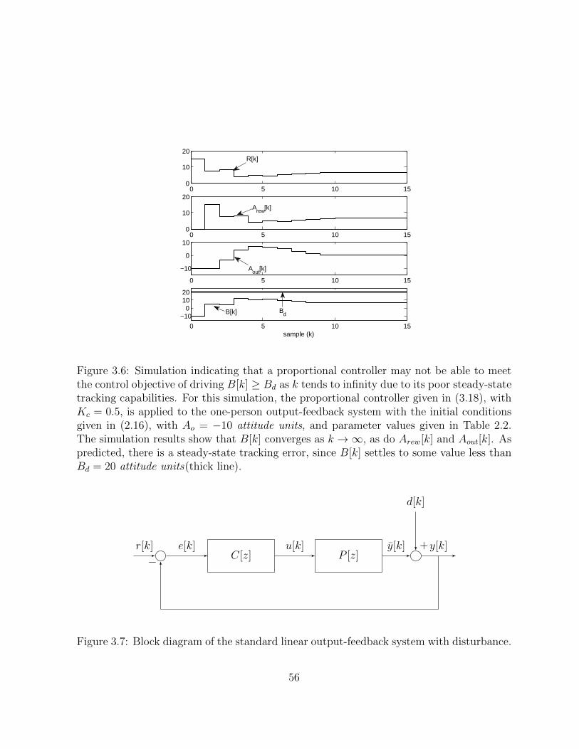
0 5 10 150

10

20

0 5 10 150

10

20

0 5 10 15

−10

0

10

0 5 10 15

−100

1020

sample (k)

R[k]

Aout[k]

B[k] Bd

Arew[k]

Figure 3.6: Simulation indicating that a proportional controller may not be able to meetthe control objective of driving B[k] ≥ Bd as k tends to infinity due to its poor steady-statetracking capabilities. For this simulation, the proportional controller given in (3.18), withKc = 0.5, is applied to the one-person output-feedback system with the initial conditionsgiven in (2.16), with Ao = −10 attitude units, and parameter values given in Table 2.2.The simulation results show that B[k] converges as k →∞, as do Arew[k] and Aout[k]. Aspredicted, there is a steady-state tracking error, since B[k] settles to some value less thanBd = 20 attitude units(thick line).

C[z] P [z]

d[k]

u[k]r[k] e[k] y[k] +y[k]

−

Figure 3.7: Block diagram of the standard linear output-feedback system with disturbance.

56

C[z] µ1

z

1z−1

∆Aout[k]

R[k]Bd e[k] Arew[k]

Aout[k]

+ B[k]

−

Figure 3.8: Block diagram of the one-person output-feedback system. The linear plantconverts the control signal, i.e., the reward, to a reward attitude. The disturbance, whicharises from the nonlinear plant dynamics, forms the internal attitude. Summing these twoattitudes generates the behavioural intent, which is fed back and compared against thedesired behaviour, Bd. The resulting error signal is used by the controller, C[z], to updatethe reward. The control signal, R[k], is given by (3.21).

attitude changes, i.e.,

Aout[k] = Ao +k−1∑i=0

∆Aout[i].

The summation term can be modelled with a discrete-time transfer function:

Aout[z]

∆Aout[z]=

1

z − 1,

with the non-zero initial condition Aout[0] = Ao. Integrating P [z] and the disturbancemodel into the standard output-feedback configuration yields the closed-loop system givenin Figure 3.8. This configuration is termed the one-person output-feedback system. Now,the problem essentially becomes a step-tracking problem, where the reference input is astep representing the desired (positive) behavioural intent, Bd > 0.

At this point, the one-person system is framed in such a way as to fit into the stan-dard linear output-feedback configuration with one complication: the disturbance, Aout[k],depends (nonlinearly) on signals within the closed-loop system. To ensure perfect steady-state tracking in the presence of step-disturbances, the feedforward system must containone summer, whereas the feedforward system must contain two summers in the case of

57

ramp-disturbances. To determine if Aout[k] can be approximated as a step-disturbance ora ramp-disturbance, the effect of the initial conditions on the system behaviour is examinedand the following assumption is made:

Assumption 3.1. The mental processing pole location for dissonance pressure in (2.11)is zero, i.e., r2 = 0.

The above assumption is made to simplify the analysis of the output-feedback analysisand thus, is specific to this section. All simulations in this section still use the mentalprocessing pole location for dissonance pressure given in Table 2.2. A direct consequenceof Assumption 3.1 is that PCD[k] = PCD

raw [k] and thus, from Lemma 2.1, PCD[k] has amaximum magnitude.

From the initial conditions on the attitudes, i.e., Aout[0] = Ao and Arew[0] = 0, theoutput, B[k], is initially negative. Suppose the controller produces a reward that is toosmall to drive behaviour positive. Previous analysis has demonstrated that in this case,attitude change occurs due to dissonance pressure alone, causing Aout[k] to decrease. Sincein this case, dissonance pressure is the only pressure contributing to attitude change, itfollows from Assumption 3.1 that this attitude change is bounded. To see why, noticethat since no overjustification pressure arises, the attitude change is simply proportionalto the dissonance pressure, which is bounded. In other words, the disturbance experiencedin the one-person output-feedback system is bounded by a ramp-function with a slopecorresponding to the maximum possible attitude change.

If, on the other hand, the controller produces a reward that is large enough to drivebehaviour positive, then initially, the only pressure experienced is dissonance pressure(since Ao < 0). Like the previous case, this dissonance pressure produces an internalattitude change, which is bounded by a ramp-function. However, unlike the case of asmall reward, the large reward potentially produces enough dissonance pressure to causeAout[k] ≥ 0, in which case overjustification pressure may arise. Should this situation occur,by Assumption 3.1, PCD[k] = 0 and therefore, only overjustification pressure arises. Asthe overjustification pressure causes Aout[k] to decrease but ensures Aout[k] ≥ 0, it followsthat ∆AOJout[k] is bounded. In conclusion, changes to Aout[k] at each sample are boundedand as a result, Aout[k] can be bounded by a ramp function.

Before proceeding, a technical detail is addressed. Since Aout[k] can both increase anddecrease, saying that Aout[k] can be bounded by a ramp function is ambiguous. In reality,this claim is composed of two different statements. First, if Aout[k] is an increasing functionof k, then it can be bounded from above by a ramp function. Alternatively, if Aout[k] isa decreasing function of k, then it can be bounded from below by a ramp function. Inthe case when Aout[k] switches from being an increasing function to a decreasing function(or vice versa), it does not make sense for one ramp function to bound Aout[k]; thus,

58

this switch means the bounding ramp function also switches. From a control perspective,switching the slope of a ramp-disturbance influences the controller’s ability to achieveperfect steady-state tracking. A double summer ensures perfect steady-state tracking fora constant ramp but does not guarantee that tracking is achieved if the slope of the rampchanges. Nevertheless, the boundedness of ∆Aout[k] is simply used as motivation for thecontroller design and therefore, this issue is not considered in more detail.

Since Aout[k] is at worst a ramp-function, and from before, perfect steady-state trackingof a linear plant with a ramp-disturbance is possible only when two summers are in thefeed-forward system, consider

C[z] =Kc

(z − 1)2 .

Before proceeding, two important details are examined: closed-loop stability and the re-quirement that Arew[k] cannot be negative.

To study the closed-loop stability of the one-person output-feedback system with theabove controller, a simplification is made: the disturbance Aout[k] is assumed to be ex-actly a ramp function. In particular, the simplifying assumption reduces the problemto considering the closed-loop stability of the system given in Figure 3.9, called the ap-proximated one-person output-feedback system or simply the approximated output-feedbacksystem. Closed-loop stability of the approximated output-feedback system is studied usingroot locus techniques. The root locus plot of P [z]C[z] is shown in Figure 3.10. This plotclearly demonstrates that for the given plant-controller combination, it is not possible tostabilize the approximated output-feedback system since any gain Kc > 0 is not able toensure that the closed-loop poles, initially located at z = 1, are contained within the unitdisk. To provide closed-loop stability of the approximated output-feedback system, a zerois included in the controller; thus, suppose

Cnom[z] =Kc (z − a)

(z − 1)2 . (3.20)

Finding the range of values for Kc and a that guarantee closed-loop stability of the ap-proximated output-feedback system is performed later in this section (see Theorem 3.9).

The second detail to discuss is the requirement that Arew[k] ≥ 0. To meet this re-quirement, a saturator and anti-windup scheme are included in the controller. Note that,Cnom[z] = R[z]

E[z], which, using the above equation for Cnom[z], can be converted into a

difference equation:

R[k] = Kce[k − 1]−Kcae[k − 2] + 2R[k − 1]−R[k − 2].

Applying the anti-windup saturator gives the follow control law:

R[k] = max {0, Kce[k − 1]−Kcae[k − 2] + 2R[k − 1]−R[k − 2]} . (3.21)

59

C[z] P [z]

ramp

R[k]Bd e[k] + B[k]

−

Figure 3.9: Block diagram of the approximated output-feedback system. The plant, P [z],is given by (3.19) and the controller, C[z], is given by (3.20). The ramp disturbancerepresents the worst possible amount of attitude change that can occur.

Real Axis

Imag

inar

y A

xis

−3 −2 −1 0 1 2 3−3

−2

−1

0

1

2

3

Figure 3.10: The root locus plot of P [z]C[z] demonstrates that the closed-loop systemof P [z]C[z] is unstable for any controller gain. Parameter values used are those given inTable 2.2.

60

Before detailed analysis is performed, a high level examination of the trends exhibitedby the one-person output-feedback system is presented. This high-level overview not onlyindicates that the controller in (3.21) may be able to meet the control objective of drivingB[k] ≥ Bd as k tends to infinity, but also provides stepping-stones used in the analysis.

At a high-level, when the controller given in (3.21) is applied to the one-person output-feedback system, the closed-loop system undergoes three stages:

I: For 0 ≤ k ≤ k − 1, Aout[k] < 0 and B[k] ≤ 0

II: For k ≤ k ≤ k − 1, Aout[k] < 0 and B[k] > 0, and

III: For k ≥ k, Aout[k] ≥ 0 and B[k] ≥ 0.

The switching from stage I to stage II occurs at k = k, whereas the switching from stageII to stage III occurs at k = k.

In stage I, the fact that B[k] is non-positive means the control signal should work toincrease B[k], resulting in a positive reward, R[k] > 0. If this reward is large enough toproduce a positive behaviour, then the system enters stage II. On the other hand, in thecase of smaller rewards, the system may continue in stage I, in which case, the positivereward attitude generated by R[k] > 0 is inconsistent with the non-positive behaviour,causing dissonance pressure to arise. Note that no overjustification pressure arises andtherefore dissonance is the only pressure contributing to attitude change. This attitudechange is in the negative direction due to the negative behaviour. Although this situationdoes not seem promising, the controller is designed to provide steady-state tracking andthus, eventually the controller should generate a R[k] that is sufficiently large to drivebehaviour positive, in which case, the system enters stage II. In fact, Lemma 3.5 presentssufficient conditions for ensuring the system enters stage II.

In stage II, the behaviour is positive but the internal attitude is still negative andtherefore, no overjustification pressure arises. However, owing to the sign change of B[k],the dissonance pressure becomes positive, but again, is bounded. In other words, theinternal attitude increases by at most a bounded rate and therefore, the assumption thatAout[k] is a ramp-disturbance still holds and therefore perfect steady-state tracking stillseems reasonable. Moreover, since attitude is increasing, it may become positive, thusplacing the system in stage III.

In stage III, the fact that Aout[k] ≥ 0, B[k] ≥ 0 and Arew[k] ≥ 0 means overjustificationpressure arises. Furthermore, by Assumption 3.1, PCD[k] = 0 (because PCD

raw [k] = 0 whenall cognitions are positive); thus, overjustification pressure is the only pressure contributingto attitude change. Previous analysis demonstrates that overjustification pressure cannotdrive attitude negative and therefore, attitude change is, again, bounded. Furthermore,

61

since Aout[k] remains positive, it follows that once the system enters stage III, it remainsin stage III; hence, provided the system is closed-loop stable, the controller should achieveperfect steady-state tracking in this stage III.

At a high-level, the controller given in (3.21) seems promising in its ability to meetthe control objective. To proceed with the analysis, closed-loop stability of the systemis first examined; then, the system characteristics for each of the three aforementionedstages are investigated. Results ensuring the system transitions through these stages toultimately reach stage III are given throughout. Once the system reaches stage III, fourpossible output trends are studied. Two of these trends are shown to be impossible, andone is shown to occur when the system is closed-loop unstable. A final conjecture ispresented indicating that if the system is closed-loop stable, then upon entering stage III,the controller is able to provide perfect steady-state tracking of the desired behaviour, Bd.

3.2.3 Output-Feedback Controller Analysis

To begin the formal analysis, closed-loop stability is examined in the context of the ap-proximated output-feedback system given in Figure 3.9. Since the controller is designedto reject ramp-like disturbances, the stability of the approximated output-feedback systemdepends on the characteristic polynomial of the closed-loop system composed of P [z] andCnom[z]. The closed-loop stability of the approximated one-person output-feedback systemis considered over that of the actual one-person output-feedback system for simplificationpurposes. The motivation for this simplification is two-fold. The primary reason for thissimplification is that if the controller given in (3.20) is unable to provide closed-loop sta-bility for the approximated output-feedback system, then the likelihood that the morerestrictive controller given in (3.21) is able to provide this stability is low. Secondly, theapproximated output-feedback system assumes a ramp-disturbance, which is considered tobe a worst-case scenario for the actual disturbance generated by Aout[k]. Using a modifiedRouth-Hurwitz approach, the theorem below gives the range of permissible gains (Kc) andzeros (a) that provide closed-loop stability of approximated output-feedback system.

Theorem 3.9. For the approximated one-person output-feedback system containing thecontroller given in (3.20), if for a ∈ (0.5, 1), Kc satisfies

0 < Kc < min

{4

µ1 (1 + 3a),2a− 1

µ1a2

},

then the closed-loop system is stable.

Proof. The proof, found in Appendix D.12, uses the Routh-Hurwitz stability test on abilinear transformation of the closed-loop system’s characteristic polynomial.

62

The conditions of Theorem 3.9 are sufficient to ensure closed-loop stability of the ap-proximated output-feedback system. To determine if the controller given by (3.21) is ableto meet the control objective, the dynamic performance of the system is studied throughconsideration of trends exhibited in each of the three aforementioned stages. In the firststage, both the behaviour and the internal attitude are negative. Since the goal is to meeta desired, positive behaviour, the controller must necessarily drive B[k] > 0. SupposeB[k] > 0 at k = k while for 0 ≤ k < k, B[k] ≤ 0. As previously discussed, the rewardprovided by the control signal either causes B[k] to increase (if the reward is large enoughto drive behaviour positive) or decrease (if the reward is too small). To guarantee B[k]eventually switches from being negative, it is enough to find conditions to ensure that B[k]becomes an increasing function of k until (at least) B[k] > 0. To this end, define T ∗ < kto be the first sample at which B[T ∗ + 1] > B[T ∗]. The lemma below states T ∗ existsand gives sufficient conditions to ensure B[k] is an increasing function of k for at least theinterval T ∗ ≤ k ≤ k.

Lemma 3.5. If the one-person output-feedback system with initial conditions given in(2.16), contains the controller given in (3.21) with zero initial conditions, then T ∗ exists.Moreover, if

Bd >K1

2µ1Kc

, (3.22)

then B[k] is an increasing function of k for at least the interval T ∗ ≤ k ≤ k, eventuallybecoming positive at k = k.


Lemma 3.5 states that as long as the desired behaviour, Bd, is large enough, then onceB[k] begins increasing, it remains an increasing function of k at least until B[k] becomespositive. Since PCD[k] < 0 for 0 ≤ k < k (due to the sign of B[k] over this interval),Aout[k] < 0 for 0 ≤ k ≤ k. Therefore, B[k] necessarily becomes positive before Aout[k] canbecome positive. Consequently, provided Bd is large enough, the system is guaranteed totransition from stage I to stage II (and not to stage III). The simulation results shown inFigure 3.11 confirm this result. Figure 3.11 contains simulation results of three differentsituations. The left-hand side plots show the behaviour and the internal attitude for asimulation using the strategy of Lemma 3.5. In this simulation, the condition given in(3.22) is met and B[k] not only starts increasing immediately, but continues increasinguntil after B[k] > 0. However, the sufficient condition given by Lemma 3.5 is conservativebecause it is derived assuming the maximum amount of dissonance pressure occurs at eachsample, which is generally not the case. The simulation results shown in the middle plotsof Figure 3.11 suggest that it is still possible for B[k] to remain an increasing function whenthe condition given by Lemma 3.5 is not met. For this simulation, Bd = 40 attitude units,

63

K1 = 30, Kc = 0.3 and µ1 = 1; thus, (3.22) is not met. Nevertheless, B[k] not only beginsto increase immediately, but B[k] continues increasing until after it becomes positive.

Not only does Lemma 3.5 provide a conservative condition for guaranteeing B[k] be-comes positive, the strategy of ensuring B[k] remains an increasing function is also con-servative. In particular, it is still possible for the system to enter stage II in the case whenB[k] does not remain an increasing function after the first sample at which it increases.The simulation results shown in the right-hand side plots of Figure 3.11 support this claim.For this simulation, the condition given in (3.22) is not met. Moreover, even though B[k] isan increasing function for 0 ≤ k ≤ 5, it becomes a decreasing function of k for 5 < k ≤ 11before again becoming an increasing function and, at k = 26, becoming positive. There-fore, the strategy to ensure B[k] remains an increasing function once it begins increasingis not necessary for ensuring the system enters stage II.

Nevertheless, Lemma 3.5 provides conditions that guarantee the system enters stage II;thus, suppose the system enters stage II at k = k, i.e., B[k] > 0 at k = k but B[k] ≤ 0for 0 ≤ k < k. In the ideal situation, B[k] > 0 for k ≥ k. However, simulation resultsdemonstrate that it is possible for the system to switch back into stage I. In fact, theclosed-loop system can display three possible trends, shown in Figure 3.12. The first trend,displayed in the top plot in Figure 3.12, is the ideal situation in which, upon switchingpositive, behaviour remains positive. Once B[k] becomes positive, it remains positive.The middle plot of Figure 3.12 shows the second trend, in which the behaviour eventuallyremains positive. This trend is acceptable, although the switching characteristics of B[k]are undesirable due to additional complications arising in the analysis. The last trend,displayed in the bottom plot of Figure 3.12, demonstrates that the behaviour could remainoscillating between positive and negative values as k tends to infinity. Extensive simulationssuggest that this final trend occurs only for smaller controller gains and small values forBd or if the controller parameters do not satisfy the conditions of Theorem 3.9.

Finding conditions to guarantee B[k] > 0 for k ≥ k is quite difficult. However,Lemma 3.5 suggests Bd err on the side of being large to ensure the system enters stageII, and since simulation results indicate larger values of Bd lead to less switching betweenstage I and stage II, it is reasonable to make the following assumption:

Assumption 3.2. The controller given in (3.21) can be tuned such that upon enteringstage II, the one-person output-feedback system never returns to stage I, i.e., B[k] > 0 fork ≤ k < k and B[k] ≥ 0 for k ≥ k.

By Assumption 3.2, the system either remains in stage II or enters stage III. Recallthat to enter stage III, Aout[k] must become non-negative. Due to being in stage II, thebehaviour is positive and therefore, the dissonance pressure that arises causes Aout[k] toincrease. This increase could drive Aout[k] ≥ 0, or could potentially lead to attitude

64

0 500

100

200

300

400

0 50

−400

−300

−200

−100

0

0 50

−100

0

100

sample (k)

0 500

100

200

300

400

0 50

−400

−300

−200

−100

0

0 50

−100

0

100

sample (k)

0 500

100

200

300

400

0 50

−400

−300

−200

−100

0

0 50

−100

0

100

sample (k)

B[k]

Aout[k]Aout[k]

R[k] R[k]R[k]

B[k]

Aout[k]

B[k]

Figure 3.11: Simulation results demonstrating that the condition given in Lemma 3.5 isconservative. The one-person output-feedback system is simulated with the controller givenin (3.21). The desired behavioural intent is set to Bd = 40 attitude units (dashed) andthe controller zero is set to a = 0.959. The one-person system has the initial conditionsgiven in (2.16) with Ao = −40 attitude units and parameter values given in Table 2.2.The simulation is performed for three different controller gains: Kc = 0.4 (left), Kc =0.3 (middle) and Kc = 0.15 (right). The left simulation uses a controller that meetsthe sufficient condition of Lemma 3.5 and demonstrates that B[k] remains an increasingfunction in stage I, as predicted by Lemma 3.5. The middle simulation demonstrates thatthe condition in Lemma 3.5 is conservative, as the parameter values used for this simulationdo not meet the condition given in Lemma 3.5, yet B[k] remains an increasing function of k.The right simulation demonstrates that the overall strategy of B[k] remaining an increasingfunction is a conservative approach, since in the simulation B[k] does not remain increasingfunction but still becomes positive.

65

0 10 20 30 40 50 60 70 80 90 100−50

0

50

100

150

B[k

]

0 10 20 30 40 50 60 70 80 90 100−50

0

50

100

150

B[k

]

0 10 20 30 40 50 60 70 80 90 100−50

0

50

100

150

sample (k)

B[k

]

Figure 3.12: Simulation results indicating three possible trends for B[k] when the systementers stage II. The one-person output-feedback system is simulated with the controllergiven in (3.21). The desired behavioural intent is set to Bd = 5 attitude units (dotted).The one-person system has the initial conditions given in (2.16) with Ao = −40 attitudeunits and parameter values given in Table 2.2. The simulation is performed for threecontroller parameter value sets: Kc = 0.4, a = 0.75 (top), Kc = 0.4, a = 0.6 (middle)and Kc = 0.1, a = 0.6 (bottom). The first controller demonstrates that once B[k] > 0,it remains positive. The second controller demonstrates that even though B[k] switchesbetween positive and negative values, the controller is eventually able to ensure B[k] > 0after some specific sample. The final controller shows that it is possible for a controller thatmeets the conditions of Theorem 3.9 to cause B[k] to never remain exclusively positive.

66

converging to a negative constant as k tends to infinity. The following lemma states thatif Aout[k] < 0 for all k, then Aout[k] converges to zero.

Lemma 3.6. If the one-person output-feedback system, with initial conditions given in(2.16), contains the controller given in (3.21) with zero initial conditions, and, for allk ≥ k,

(i) B[k] > 0, and

(ii) Aout[k] < 0;

then Aout[k]→ 0 as k →∞.


Although Lemma 3.6 does not guarantee Aout[k] becomes non-negative, thus ensuringthe system enters stage III, it is later shown that if Aout[k] ≥ 0 at some k = k, then Aout[k]still tends to zero as k tends to infinity (see Lemma 3.9). As a result, the characteristicsof the system output, B[k], as k → ∞ are the same in the case when Aout[k] < 0 for allk ≥ 0 as when Aout[k] becomes non-negative at k = k. Thus, the analysis continues byinvestigating the system characteristics for the case when Aout[k] ≥ 0.

Suppose the system enters stage III at k = k, i.e., B[k] ≥ 0 and Aout[k] ≥ 0 (butAout[k] < 0 for 0 ≤ k < k); then, the system remains in stage III for k ≥ k becauseArew[k] ≥ 0 (due to the controller equation given in (3.21)) and Aout[k] ≥ 0 for k ≥ k.The latter claim holds from the fact that the overjustification effect cannot decrease theinternal attitude to a negative value. Furthermore, since PCD

raw [0] = 0 at k = k, it followsfrom Assumption 3.1 that PCD[k] = 0 at k = k and therefore, overjustification pressure isthe only contributor to attitude change, i.e., Aout[k] ≥ 0 for k ≥ k. Moreover, as behaviouris the sum of Arew[k] and Aout[k], both of which are non-negative for k ≥ k, B[k] ≥ 0 alsoand therefore, the system necessarily remains in stage III for k ≥ k.

Now, it only remains to determine whether or not the controller given in (3.21) is ableto drive B[k] ≥ Bd as k →∞. At this point, B[k] could display four possible trends as ktends to infinity.

• B[k] remains below Bd in the sense that there exists an ε > 0 and N such that, forall k > N , B[k] < Bd − ε.

• B[k] remains above Bd in the sense that there exists an ε > 0 and N such that, forall k > N , B[k] > Bd + ε.

• B[k] converges to Bd.

67

e[k]1

z − 1

1

z − 1Kc (z − a) max

0

R[k]e1[k] e2[k] Rus[k]

Figure 3.13: The controller given in (3.21) is expanded into several first-order components.Intermediate signals are given names to aid the analysis. The input to the controller isgiven by e[k] = Bd − B[k] and the output of the controller is the reward signal, R[k].This expanded block-diagram is used in Lemmas 3.7 and 3.10 to show that two of the fourpossible characteristics for B[k] are impossible.

• B[k] oscillates around Bd without converging, in the sense that there exists an ε > 0such that, for every N , there is a k1 > N and a k2 > N such that B[k1] > Bd + εand B[k2] < Bd − ε.

The trend of remaining below Bd is considered first. To aid the analysis, the controlleris separated into various components and intermediate signals as shown in Figure 3.13. Ata high level, this figure helps explain why, provided a mild technical condition holds, thesystem cannot exhibit the first trend, as stated in the lemma below.

Lemma 3.7. For all Bd >K1

2, if the one-person output-feedback system, with initial con-

ditions given in (2.16), contains the controller given in (3.21) with zero initial conditionsand enters stage III at k = k, then, for all ε > 0, there does not exist a k such that for allk ≥ k, B[k] ≤ Bd − ε.


Lemma 3.7 says that the one-person output-feedback behaviour signal cannot remainless than Bd as k tends to infinity provided Bd >

K1

2. To understand why this technical

condition exists, consider the state-feedback controllers in the previous section. For rela-tively small values of Bd, the controller forces R[k] = 0, whereas larger Bd values requirepositive reward, as the internal attitude cannot alone produce the desired behaviour. Inthe same vein, the technical condition in Lemma 3.7 simplifies the analysis by forcing thecontrol signal to always be positive. As a result, not only is a positive reward necessaryfor achieving the control objective, R[k] cannot converge to zero as k tends to infinity, asstated in the lemma below.

68



ditions given in (2.16), contains the controller given in (3.21) with zero initial conditionsand enters stage III at k = k, then R[k] cannot converge to zero as k tends to infinity.


Not only does Lemma 3.8 conclude that, as k →∞, a reward is necessary for achievingthe control objective, it can be used to show two more conclusions relevant to the system’scharacteristics. First, the fact that R[k] cannot converge to zero as k → ∞ helps showthat Aout[k] necessarily converges to zero as k tends to infinity as stated in the followinglemma.



ditions given in (2.16), contains the controller given in (3.21) with zero initial conditionsand enters stage III at k = k, then

Aout[k]→ 0 as k →∞.


By combining the results of Lemmas 3.6 and 3.9, we conclude that if the system entersstage II, then the internal attitude converges to zero as k tends to infinity and, therefore,the trends exhibited by B[k] as k →∞ are the same in the case when the system remainsin stage II as in the case when the system reaches stage III.

The second conclusion arising from Lemma 3.8 is Lemma 3.10 below, which says thatthe second of the four aforementioned trends for B[k] is impossible.


2, if the one-person output-feedback system, with initial

conditions given in (2.16), contains the controller given in (3.21) with zero initial conditionsand enters stage III at k = k, then, for any ε > 0, there does not exists a k such that forall k ≥ k, B[k] ≥ Bd + ε.


The results of Lemmas 3.7 and 3.10 are conditional on the system eventually enteringstage III. However, Lemmas 3.6 and 3.9 show that in both the case when the system remainsin stage II and when the system reaches (and remains in) stage III, Aout[k] converges tozero as k tends to infinity. Consequently, the trends exhibited by B[k] as k → ∞ are thesame in both cases. The theorem below summarizes these results.

69

Theorem 3.10. For all Bd >K1

2, if the one-person output-feedback system, with initial

conditions given in (2.16), contains the controller given in (3.21) with zero initial conditionsand enters stage II at k = k, then, for any ε > 0, there does not exist a k such that

(a) B[k] ≥ Bd + ε for all k ≥ k, or

(b) B[k] ≤ Bd − ε for all k ≥ k.

Proof. The theorem follows immediately from Lemmas 3.6, 3.7, 3.9 and 3.10.

There are now two remaining possible trends that could be exhibited by B[k]: oscillationaround Bd or convergence to Bd as k tends to infinity. We first consider the case whenB[k] oscillates.

Consider the parameters a and Kc, which are common to the controller of both theapproximated and actual output-feedback systems ((3.20) and (3.21) respectively). Giventhat (3.21) is more restrictive than (3.20) (because of the additional saturator and anti-windup scheme in (3.21)), it is reasonable to suggest that if a andKc do not provide stabilityfor the approximated system, these same parameters are unlikely to provide stability forthe actual system. Since Theorem 3.10 does not assume the system is closed-loop stable,two of the three potentially unstable trends have been eliminated, i.e., B[k] cannot tendto positive or negative infinity as k → ∞ because B[k] cannot remain above or below Bd

as k tends to infinity. Thus, the remaining unstable trend, oscillation around Bd, is likelyto occur only if the conditions of Theorem 3.9 fail to hold, whereas the desirable outcomeof B[k] converging to Bd as k tends to infinity is likely to occur only if the conditions ofTheorem 3.9 hold. This hypothesis is summarized in the conjecture below.

Conjecture 3.1. For all Bd >K1

2, suppose the one-person output-feedback system, with

initial conditions given in (2.16), contains the controller given in (3.21) with zero initialconditions and enters stage II at k = k. If the controller parameters do not satisfy theconditions of Theorem 3.9, then B[k] oscillates around Bd as k →∞. On the other hand,if the controller parameters satisfy the conditions of Theorem 3.9, then B[k] tends to Bd

as k →∞.

Figure 3.14 below presents simulations supporting Conjecture 3.1 and Theorem 3.10. Inthese simulations, the controller is tuned to ensure Assumption 3.2 is met. Both simulationresults are consistent with Theorem 3.10 because both demonstrate that B[k] does notremain above or below Bd as k tends to infinity. In the left simulation, the controllerparameters used satisfy the conditions of Theorem 3.9. Since these simulation results showB[k] converges to Bd as k tends to infinity, they provide evidence to support Conjecture 3.1.Furthermore, in the simulation shown on the right-hand side of Figure 3.14, the controller

70

0 50 1000

100

200

0 50 1000

100

200

0 50 100−40

−20

0

0 50 100−50

0

50

100

150

sample (k)

0 50 1000

100

200

0 50 1000

100

200

0 50 100−40

−20

0

0 50 100−50

0

50

100

150

sample (k)

R[k]

Arew[k] Arew[k]

Aout[k] Aout[k]

R[k]

B[k] B[k]

Figure 3.14: Simulation of the one-person output-feedback system with initial conditionsgiven in (2.16), controller given in (3.21) and parameter values given in Table 2.2. Bothsimulations use an initial attitude Ao = −40 attitude units, desired behaviour Bd = 40attitude units, and controller zero, a = 0.65. Using these parameter values, the approxi-mated output-feedback system is stable when Kc < 0.71. In the left simulation, Kc = 0.5.The system enters stage III at k = 10 because B[k] ≥ 0 and Aout[k] ≥ 0 for k ≥ 10. AsConjecture 3.1 hypothesizes, as k tends to infinity, B[k] converges to Bd (denoted by thedotted line). The right simulation provides additional support for Conjecture 3.1. In thissimulation Kc = 0.72, and, therefore, the conditions of Theorem 3.9 are not met. Thesystem enters stage III at k = 10, and the output, B[k], oscillates around the desiredbehaviour, Bd, again denoted by the dotted line. Both simulations demonstrate the resultsof Theorem 3.10 by showing B[k] cannot remain above or below Bd as k tends to infinity.

71

parameters do not meet the conditions of Theorem 3.9, and the output signal, B[k], isshown to oscillate around Bd as k tends to infinity, thus supporting Conjecture 3.1.

Although showing that the controller given in (3.21) can meet the control objective forany set of initial conditions is currently an open problem, there is evidence to suggest thatthis is the case. Note that the approximation on the nonlinear disturbance in Figure 3.9still holds for any set of initial conditions. To see why, recall that this disturbance isthe internal attitude, Aout[k]. To show that changes to Aout[k] are bounded, we arguethat ∆Aout[k] is bounded. From (2.5), ∆Aout[k] is the sum of two signals, ∆ACDout [k] and∆AOJout[k]. By Lemma 2.1, −0.5 ≤ PCD

raw [k] ≤ 0.5 and therefore, PCDraw [k] is bounded. Since

PCD[k] = r2PCD[k−1]+(1− r2)PCD

raw [k] is BIBO stable, it follows that PCD[k] is bounded.As a result, ∆ACDout [k] is also bounded. Next, consider ∆AOJout[k]. If raw overjustificationpressure exists at times k ≥ k, then Aout[k], Arew[k] and B[k] are all positive for k ≥ k.This result implies that PCD

raw [k] = 0 for k ≥ k, meaning PCD[k] tends to zero as k tendsto infinity. Also, due to the signs in (2.13)–(2.15), ∆AOJout[k] ≤ 0. As a result, Aout[k] isbounded above for k ≥ k. Finally, from (2.15), Aout[k] ≥ 0 for k ≥ k and thus, Aout[k] isbounded. Therefore, the nonlinear disturbance can be approximated with a ramp for anyset of initial conditions; hence, the following conjecture is made.

Conjecture 3.2. For all Bd > 0, if the one-person output-feedback system contains thecontroller given in (3.21), then the controller parameter values can be selected to ensure

B[k]→ Bd as k →∞.

To provide further evidence of Conjecture 3.2, a set of 200 simulations is performed. Foreach of the 200 simulations, random values are given to Bd, the initial conditions (bothof the model and the controller), and the model parameters (according to the restrictionsin Table 2.2). Then the controller parameters are chosen to meet the condition given inTheorem 3.9. In each simulation, the output, B[k], converges to Bd as k →∞. Figure 3.15shows the simulation results for one of the tests.

To summarize, this chapter studied various open-loop and closed-loop controllers tomeet the control objective of driving B[k] ≥ Bd as k tends to infinity. Two open-loopcontrollers were considered: an impulse reward and a step reward. The impulse-rewardcontroller was shown to be able to increase B[k] but is unable to meet the control objectivefor all combinations of Ao, Bd and K1, unlike the step-reward controller. Although thestep-reward controller is able to meet the control objective, the undesirable consequenceof the reward on the internal attitude motivated studying closed-loop controllers. Thefirst, a state-feedback controller, was the extended-impulse-reward controller, where thereward signal is removed immediately before the internal attitude becomes non-negative.Although this controller is unable to always satisfy the goal of driving B[k] ≥ Bd as k tendsto infinity, its use of state-feedback motivated a more general state-feedback controller.

72

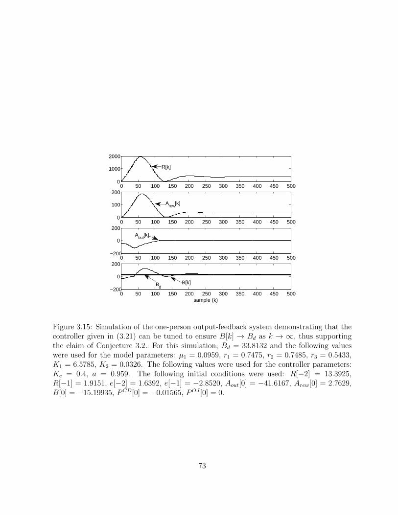
0 50 100 150 200 250 300 350 400 450 5000

1000

2000

0 50 100 150 200 250 300 350 400 450 5000

100

200

0 50 100 150 200 250 300 350 400 450 500−200

0

200

0 50 100 150 200 250 300 350 400 450 500−200

0

200

sample (k)

R[k]

BdB[k]

Arew[k]

Aout[k]

Figure 3.15: Simulation of the one-person output-feedback system demonstrating that thecontroller given in (3.21) can be tuned to ensure B[k] → Bd as k → ∞, thus supportingthe claim of Conjecture 3.2. For this simulation, Bd = 33.8132 and the following valueswere used for the model parameters: µ1 = 0.0959, r1 = 0.7475, r2 = 0.7485, r3 = 0.5433,K1 = 6.5785, K2 = 0.0326. The following values were used for the controller parameters:Kc = 0.4, a = 0.959. The following initial conditions were used: R[−2] = 13.3925,R[−1] = 1.9151, e[−2] = 1.6392, e[−1] = −2.8520, Aout[0] = −41.6167, Arew[0] = 2.7629,B[0] = −15.19935, PCD[0] = −0.01565, POJ [0] = 0.

73

This second state-feedback controller is not only able to meet the goal as k → ∞, it isable to meet the goal immediately, for k ≥ 1, while also maintaining internal stability.However, due to the impractical nature of state-feedback for the given application, anoutput feedback controller was then considered. Since the one-person output-feedbacksystem can be framed as a linear output-feedback system with a disturbance, linear controltechniques were used to design this final controller. In particular, the disturbance wasapproximated to be a ramp. The output-feedback controller was then designed usinglinear control techniques to attain perfect steady-state tracking and perfect steady-stateramp-disturbance rejection. The analysis given showed that the system passes throughthree stages, eventually reaching a stage with only two possible outcomes. Supported byextensive simulation results, a final conjecture hypothesizes that B[k] necessarily convergesto Bd as k → ∞ if the approximated system is stable, whereas B[k] necessarily oscillatesaround Bd if the approximated system is unstable. The results presented in this chapter arenot only useful for control of the one-person system, but also motivate design approachestaken in Chapter 5 when control of the two-person system is investigated.

74

Chapter 4

Two-Person System:Psychology and Modelling

In the one-person system, a person with an initially negative attitude is offered a reward inan attempt to overtly control the person’s behaviour. This person does not experience anyother external influences. This assumption is idealistic since an individual may experiencesocial influences from a variety of sources including friends, peers, society and media;hence, this assumption is now relaxed. In particular, we now assume that, in additionto the external influence of a reward, an individual experiences a social influence fromthe behaviour of another person. In the context of the piano situation, the child’s friendrepresents this additional person. The friend’s behaviour influences the child’s attitude andbehaviour and, likewise, the child’s behaviour influences his friend. Thus, the two-personsystem consists of attitude-behaviour models of two individuals, connected in some waythrough the behaviour of these two individuals.

To model this connection and its effect on attitude and behaviour, additional psychol-ogy background is required. From the theory of planned behaviour, three elements combineto generate a behaviour, one of which is external influences. The one-person system dealswith only one external influence, rewards. However, the theory of planned behaviour ex-tends beyond rewards and models how two general categories of external influences affectan individual’s behaviour. These categories, termed social pressure and conformity pres-sure, are explained in Sections 4.1.1 and 4.1.2 respectively. Provided in these explanationsis a discussion of how these pressures relate to cognitive dissonance theory and the over-justification effect. Following this discussion, a two-person discrete-time dynamic model isderived using the framework given in Chapter 2. The model is then verified to be qualita-tively consistent with the psychology. Finally, other psychological phenomena arising fromgroup dynamics are introduced and discussed within the context of the two-person system.

75

4.1 Psychology Describing the Influence of

Other People

In Chapter 2, the effect of external influences is not fully captured. For the one-personsystem, the external influence is simply a reward. However, the theory of planned behaviourextends beyond the effect rewards have on an individual’s behaviour. The theory capturesthe effects of two general categories of external influences, which for the thesis are termedsocial pressure and conformity pressure. These two influences, studied, among others, byAjzen in [11], are defined below:

1. Social pressure: Influence arising from the perception of “what should or ought tobe done with respect to performing a given behaviour.”

2. Conformity pressure: Influence arising from the perception “that others are orare not performing the behaviour in question.”

The external influence in the one-person system, a reward, is a special case of socialpressure, as the presence of a reward is accompanied by the expectation of performinga given behaviour. The two-person system contains external influences from both of thesecategories; hence, each are now discussed in more detail.

4.1.1 Social Pressure

Social pressure refers to pressures arising from perceptions of the expectations other peoplehave of an individual carrying out a particular behaviour. For example, a child may perceivethat other people, such as his teachers, friends and/or parents, want him to play the piano.If the child perceives that his teachers strongly want him to play the piano, then the socialpressure experienced by the child, denoted P SP [k], is high, i.e., P SP [k]� 0. On the otherhand, if the child perceives that his teachers strongly want him to not play the piano, thenP SP [k]� 0. The sign of P SP [k] indicates whether the expectation is to play or to not playthe piano, whereas the magnitude |P SP [k]| indicates the social pressure strength. Notethat P SP [k] is not the actual expectation of another person, but instead, is an individual’sperception of this expectation.

Research suggests that even though social pressure may arise, it does not necessarilyinfluence the behaviour of an individual. A second component is thus needed to transformthis social pressure into an attitude and, consequently, into behaviour. This componentreflects the value an individual places on the wishes of the person exerting the socialpressure and is denoted in our model by µ2. For example, suppose the child experiencesstrong social pressure from his teachers. If he does not care about the wishes of his teachers,

76

then the influence this social pressure has on the child’s attitude is small, whereas thisinfluence is larger in the case when the child cares about the expectations of his teachers.The value placed on the wishes of the individual exerting this pressure combines with thesocial pressure, P SP [k], through a product, forming the attitude towards a behaviouraloutcome that arises from social pressure due to other people, denoted Aothers[k]. If morethan one person is applying social pressure, then Aothers[k] is the sum of the attitudes arisingfrom the social pressure applied by each individual. That is, the social pressure exerted byperson n, P SP

n [k], and the degree to which the individual cares about the expectations ofperson n, µ2n, combine over N people to form Aothers[k] as follows:

Aothers[k] =N∑n=1

P SPn [k]µ2n.

The above sum excludes social pressure that arises from rewards because our model al-ready has a specific mechanism in place to generate a reward attitude. This mechanism isconsistent with the above formation of Aothers[k] (see (2.3)). The two attitudes are differ-entiated because, later, rewards are the only social pressure considered in the two-personmodel and Arew[k] provides intuitive notation.

Not only does social pressure directly influence behaviour through the theory of plannedbehaviour, the related attitude, Aothers[k], is a cognition, much like Aout[k] and Arew[k].As such, it forms a cognitive pair with the generative cognition, B[k], and potentiallycontributes to dissonance pressure and overjustification pressure. From the psychology lit-erature, overjustification pressure arises in a very specific paradigm: it assumes a reward isused to control the behaviour of an individual with a pre-existing positive attitude towardsthe behaviour, i.e., Aout[k] > 0, Arew[k] > 0 and B[k] > 0. Since rewards are a special caseof social pressure, the following assumption is made to extend the overjustification effectpsychology to the more general social pressure:

Assumption 4.1. Any type of social pressure can produce overjustification pressure.

Following the way in which Arew[k] leads to overjustification pressure, if all cognitive pairsare consistent, we model that if Aothers[k] = 0 then no overjustification pressure arises; onthe other hand, if Aothers[k] > 0, then overjustification pressure arises because the childattributes his behaviour to being overtly controlled by other people as opposed to his owninternal attitude. If any cognitive pair is inconsistent, then overjustification pressure doesnot arise and, instead, dissonance pressure arises. In this case, the amount of dissonancepressure experienced is formed as described in Section 2.2.1, i.e.,

P =

∑Mincon∑

Mincon +∑Mcon

.

77

To summarize, one type of external influence on an individual’s behaviour is socialpressure, which forms a related attitude. In the case of rewards, this attitude is given byArew[k], whereas for more general social pressure, given by P SP [k], the related attitudeis given by Aothers[k]. Both Arew[k] and Aothers[k] form cognitive pairs with B[k] and cancontribute to dissonance and overjustification pressures. It is through the reward thatsocial pressure is considered in this thesis. The effect of Aothers[k] on the internal attitudeand the behaviour of an individual is an item for future, related work and is included inthe model for completeness.

4.1.2 Conformity Pressure

If other, significant people are performing the behaviour, then an individual is more likelyto also perform the behaviour. This is the well-known psychological theory of conformity,which Myers and Spencer, in [14], describe as the “change of behaviour or belief to accordwith others.” This description raises an interesting observation: conformity can influ-ence both the behaviour and the attitude of an individual. Indeed, psychology literatureseparates conformity into two cases [14]:

1. Compliance: When an individual carries out the given behaviour because other peo-ple carry out the behaviour, while privately disagreeing. That is, behaviour changesbut not attitude.

2. Acceptance: When an individual carries out the given behaviour because otherpeople carry out the behaviour, and this individual changes his internal attitude tomatch. That is, both attitude and behaviour change.

Both compliance and acceptance involve change in behaviour, and the theory of plannedbehaviour offers one mechanism through which such change can occur; thus, we use thistheory as the way of modelling behaviour change arising from conformity pressures.1

From the theory of planned behaviour, when conformity pressure is experienced, aconformity attitude is formed, denoted Aconf [k]. Similar to the other attitudes in ourmodel, the conformity attitude consists of two components. The first component is thebehaviour of a second person. For our model, the behaviours of the two people are denotedB1[k] and B2[k], where the subscripts 1 and 2 differentiate between the person beingoffered a reward and the person not being offered a reward. In the context of the pianoexample, the child is person one and his friend is person two. The conformity pressure

1The original formulation of Ajzen’s theory of planned behaviour did not consider the effect of otherpeople’s behaviour. However, in [11], Ajzen states that there is plenty of evidence to suggest that thisinfluence should be included in his model.

78

experienced by the child depends on the behaviour of his friend, B2[k], and vice versa. Thesecond component of conformity attitude is the extent to which a person can be influencedby another and is denoted µ3. For our model, there are two people and µ32 representshow much the behaviour of person two influences the conformity attitude of person one,whereas µ31 represents the extent to which person one’s behaviour influences person two’sconformity attitude. These two components combine to generate a conformity attitudeand, although psychologists have yet to determine this exact relationship, in [11] Ajzenproposes the following model for the conformity attitude arising from conformity pressureexerted by N other people:

Aconf [k] =N∑i=1

µ3iBi[k].

In our model, there are two people and thus, each person experiences conformity pres-sure from one other person, i.e., N = 1. For each person in the model, the conformityattitude, Aconf,i[k], then combines (through the theory of planned behaviour) with theother attitudes, Aout,i[k], Arew,i[k] and Aothers,i[k] to produce a behaviour, Bi[k]. More-over, as Aconf,i[k] is another cognition in the two-person model, it forms a cognitive pairwith Bi[k], which is either consistent or inconsistent. If this (or any) cognitive pair in thetwo-person system is inconsistent, then dissonance pressure arises and is calculated in theusual manner.

In cases where acceptance occurs, research in the field of conformity suggests thatbehaviour changes tend to precede attitude change [14]. To model this attitude change, aswell as to ensure consistency in the order in which behaviour and attitude change, cognitivedissonance theory can be used. In [9], Festinger discusses dissonance pressure arising fromsocial situations and argues that the behaviour of others can produce dissonance pressure,which can be reduced through (internal) attitude change. Since our model includes theeffects of dissonance pressure, it already contains a mechanism through which acceptancecan occur.

The final point to consider is the effect of Aconf,i[k] on the overjustification pressure.Unlike the social pressures Arew,i[k] and Aothers,i[k], an individual does not feel overtlycontrolled through conformity pressure. Since Aconf,i[k] is not controlling in nature, thefollowing psychological assumption is made:

Assumption 4.2. Overjustification pressure cannot arise due to conformity pressure.

Note that, in particular, if the cognitive pair (Aconf,i[k], Bi[k]) is consistent and no otherinconsistencies arise, then Aconf,i[k] does not contribute to overjustification pressure.

To summarize, conformity pressure arises from one individual observing the behaviourof another. The compliance element of conformity describes how an individual’s behaviouris directly influenced by that of another person. In the context of the piano situation, the

79

Person One(Child)

Person Two(Friend)

R[k]B2[k]

B1[k]

Figure 4.1: The overall psychological system of the two-person model (dotted box), de-composed into attitude-behaviour models of each person, each of which is an augmentedone-person system, updated to include the effects of other external influences, Aconf [k] andAothers[k]. The system input is R[k] and the system outputs are B1[k] and B2[k].

behaviour of the child’s friend and the extent to which this friend can influence the childcombine to form a conformity attitude, Aconf [k]. This conformity attitude has a direct in-fluence on the child’s behaviour. Furthermore, the acceptance element of conformity, whichsays that an individual’s attitude may also change, is modelled by the existing dissonancepressure mechanism. If any cognitive pair in the two-person system is inconsistent, thendissonance pressure arises and Aconf [k] contributes to the dissonance pressure magnitudeand, thus, attitude change.

4.2 The Augmented Dynamic Feedback Model

The framework given in Section 2.3 is now used to develop the two-person discrete-timemodel. First, Component A, which models the theory of planned behaviour, is updated toinclude Aothers[k] and Aconf [k] as described in Section 4.1.1 and 4.1.2 respectively. Then,Component B, which models cognitive dissonance and the overjustification effect, is up-dated to include these two new cognitions. Component A and Component B form anupdated version of the one-person system with an additional input: the behaviour of an-other person. The two-person system, shown in Figure 4.1, is essentially composed of two,one-person models connected via behaviour. Specifically, the behaviour of one person inthe system is an input to the other person. To distinguish between the signal and parame-ter values for each person, additional subscripts are used in the notation given in Table 2.2;Table 4.1 summarizes new signals and provides the parameter values used for simulatingthe two-person system. Finally, although each one-person system allows for two inputs,for this thesis only one of the two people receives a reward input. An item for future workis to consider two input reward signals, one for each person. In the context of the pianosituation, person one is the child and person two is the child’s friend.

80

Sym

bol

Desc

ripti

on

[valueorunits]

Aothers,i[k]∈

(−∞,∞

)at

titu

de

tow

ards

the

beh

avio

ur

aris

ing

from

soci

alpre

ssure

[att

itu

deu

nit

s]Aconf,i[k

]∈

(−∞,∞

)at

titu

de

tow

ards

the

beh

avio

ur

aris

ing

from

confo

rmit

ypre

ssure

[att

itu

deu

nit

s]PSP

i[k

]∈

(−∞,∞

)so

cial

pre

ssure

[soc

ial

pres

sure

un

its]

POJ,rew

raw,i

[k],POJ,rew

i[k

]∈

[0,∞

)pre

ssure

aris

ing

from

the

over

just

ifica

tion

effec

tdue

tore

war

ds

[(at

titu

deu

nit

s)2]

POJ,others

raw,i

[k],POJ,others

i[k

]∈

[0,∞

)pre

ssure

aris

ing

from

the

over

just

ifica

tion

effec

tdue

toso

cial

pre

s-su

re[(

atti

tude

un

its)

2]

K1i∈

[0,∞

)†ga

inre

flec

ting

how

the

dis

sonan

cepre

ssure

affec

tsat

titu

de

chan

ge[K

11

=K

12

=30

atti

tude

un

its]

K2i∈

[0,∞

)†ga

inre

flec

ting

how

the

over

just

ifica

tion

pre

ssure

due

tore

war

ds

affec

tsat

titu

de

chan

ge[K

21

=K

22

=0.

11/

(att

itu

deu

nit

)]K

3i∈

[0,∞

)†ga

inre

flec

ting

how

the

over

just

ifica

tion

pre

ssure

due

toso

cial

pre

s-su

reaff

ects

atti

tude

chan

ge[K

31

=K

32

=0.

11/

(att

itu

deu

nit

)]µ

1i∈

[0,∞

)va

lue

assi

gned

toon

edol

lar

[µ11

=µ

12

=1

atti

tude

un

itpe

rdo

llar

]µ

2i∈

[0,∞

)im

por

tance

ofot

her

peo

ple

who

apply

soci

alpre

ssure

[µ21

=µ

22

=50

atti

tude

un

its

per

soci

alpr

essu

reu

nit

]µ

3i∈

[0,∞

)ex

tent

tow

hic

hp

erso

non

ein

fluen

ces

per

son

two

and

vic

eve

rsa

[µ31

=µ

32

=0.

5u

nit

less

]r 1i∈

[0,1

)†m

enta

lpro

cess

ing

pol

elo

cati

onfo

rre

war

dat

titu

de

form

atio

nin

(4.2

)[r

11

=r 1

2=

0]r 2i∈

[0,1

)†m

enta

lpro

cess

ing

pol

elo

cati

onfo

rso

cial

pre

ssure

atti

tude

form

a-ti

onin

(4.3

)[r

21

=r 2

2=

0]r 3i∈

[0,1

)†m

enta

lpro

cess

ing

pol

elo

cati

onfo

rco

nfo

rmit

yat

titu

de

form

atio

nin

(4.4

)[r

31

=r 3

2=

0]r 4i∈

[0,1

)†m

enta

lpro

cess

ing

pol

elo

cati

onfo

rdis

sonan

cepre

ssure

in(4

.16)

[r41

=r 4

2=

0.5]

Con

tinued

onN

ext

Pag

e...

81

Tab

le4.

1–

Con

tinued

Sym

bol

Desc

ripti

on

[valueorunits]

r 5i∈

[0,1

)†m

enta

lpro

cess

ing

pol

elo

cati

onfo

rre

war

dov

erju

stifi

cati

oneff

ect

in(4

.20)

[r51

=r 5

2=

0.5]

r 6i∈

[0,1

)†m

enta

lpro

cess

ing

pol

elo

cati

onfo

rot

her

sov

erju

stifi

cati

oneff

ect

in(4

.21)

[r61

=r 6

2=

0.5]

Tab

le4.

1:K

eysi

gnal

san

dpar

amet

ers

that

app

ear

inth

etw

o-p

erso

nsy

stem

.T

he

par

amet

erva

lues

list

edar

eth

ose

use

dfo

ran

alysi

sin

Chap

ter

5.P

aram

eter

sm

arke

d†

dep

end

onth

esa

mpling

per

iod,

take

nher

eto

be

one

day

.

82

4.2.1 Revising Component A

Component A models the theory of planned behaviour. The equations presented in Sec-tion 2.3.1 detail how an individual’s internal attitude and reward attitude combine toproduce a behavioural intent (see (2.2)–(2.4)). Since our model now contains two peo-ple, the attitudes and behavioural intent of each person must be represented by distinctequations; thus, let the subscripts i and j (where i = 1 and j = 2, or i = 2 and j = 1)differentiate between the attitudes and behaviours of the two individuals. In Section 4.1,two additional attitudes were considered: the attitude arising from the social pressure ex-erted by others, Aothers[k], and the attitude arising from conformity pressure, Aconf [k]. Theformer attitude depends on social pressure (P SP [k]), the importance of the people applyingthe social pressure (µ2), and a first-order mental processing model (with r2 denoting thepole location). Furthermore, the conformity attitude of person i (Aconf,i[k]) depends onthe behaviour of person j (Bj[k]), the amount of influence person j has on person i (µ3j),and again, a first order-mental processing model (with r3 denoting the pole location). Theinternal attitude and reward attitude are the same as in the one-person model. As before,the theory of planned behaviour states that the weight of each attitude varies by situationand individual; thus, for our model, this weighting is contained in µ1, µ2 and µ3, scalingthe reward, social pressure and conformity pressure into attitude units respectively. Thus,Component A for person i is now modelled by the following five equations:

Aout,i[k] = Aout,i[k − 1] + ∆Aout,i[k − 1] (4.1)

Arew,i[k] = r1iArew,i[k − 1] + µ1i (1− r1i)Ri[k − 1] (4.2)

Aothers,i[k] = r2iAothers,i[k − 1] + µ2i (1− r2i)PSPi [k − 1] (4.3)

Aconf,i[k] = r3iAconf,i[k − 1] + µ3j (1− r3i)Bj[k − 1] (4.4)

Bi[k] = Aout,i[k] + Arew,i[k] + Aothers,i[k] + Aconf,i[k]. (4.5)

4.2.2 Revising Component B

As before, Component B, shown in detail in Figure 4.2, is based on cognitive dissonancetheory and the overjustification effect. These two psychological effects create pressure,producing attitude change. Thus, the output of Component B, ∆Aout[k], remains thesame as in the one-person system:

∆Aout,i[k] = ∆ACDout,i[k] + ∆AOJout,i[k]. (4.6)

The difference between the one-person system and the two-person system lies in how theseattitude change terms are formed. Each of these terms will now be examined.

83

∆Aout,i[k]

(4.22) (4.20) (4.18)

(4.17) (4.16) (4.15)

(4.23) (4.21) (4.19)

Bi[k]Aout,i[k]Arew,i[k]Aconf,i[k]Aothers,i[k]

∆AOJ,rewout,i [k] POJ,rew

i [k] POJ,rewraw,i [k]

∆ACDout,i[k] PCD

i [k] PCDraw,i[k]

∆AOJ,othersout,i [k] POJ,others

i [k] POJ,othersraw,i [k]

∆AOJout,i[k]

Figure 4.2: Details of the revised Component B. Thick line is used to indicate multiplesignals.

Revising the Cognitive Dissonance Theory Model

For the one-person system, the induced compliance paradigm of cognitive dissonance theoryis used, resulting in simplified dissonance pressure equations. This paradigm applies whenAout[k] < 0 and Arew[k] > 0 and does not consider how other people affect dissonancepressure. As such, a more general approach is now needed for modelling the dissonancepressure. The assumption that the internal attitude is negative is dropped, while thereward attitude is still assumed to be non-negative. Recall that the dissonance pressure isthe ratio between the inconsistency magnitudes and the magnitudes of all cognitive pairsand therefore, the consistency and inconsistency magnitudes for each cognitive pair arefirst presented.

For the two-person model, person i has four attitudes, Aout,i[k], Arew,i[k], Aothers,i[k]and Aconf,i[k], each of which forms a cognitive pair with the generative cognition, Bi[k].Each cognitive pair has an associated Mcon,i[k] or Mincon,i[k]. Similar to the one-personmodel, these magnitudes are proportional to the strength of each element in the cognitive

84

pair; thus, define

M1incon,i[k] =

{|Arew,i[k]Bi[k]| if Arew,i[k] ≥ 0, Bi[k] < 0,

0 otherwise,(4.7)

M2incon,i[k] =

|Aout,i[k]Bi[k]| if Aout,i[k] < 0, Bi[k] ≥ 0,

or Aout,i[k] ≥ 0, Bi[k] < 0,

0 otherwise,

(4.8)

M3incon,i[k] =

|Aothers,i[k]Bi[k]| if Aothers,i[k] < 0, Bi[k] ≥ 0,

or Aothers,i[k] ≥ 0, Bi[k] < 0,

0 otherwise,

(4.9)

M4incon,i[k] =

|Aconf,i[k]Bi[k]| if Aconf,i[k] < 0, Bi[k] ≥ 0,

or Aconf,i[k] ≥ 0, Bi[k] < 0,

0 otherwise,

(4.10)

and

M1con,i[k] =

{|Arew,i[k]Bi[k]| if Arew,i[k] ≥ 0, Bi[k] ≥ 0,

0 otherwise,(4.11)

M2con,i[k] =

|Aout,i[k]Bi[k]| if Aout,i[k] < 0, Bi[k] < 0,

or Aout,i[k] ≥ 0, Bi[k] ≥ 0,

0 otherwise.

(4.12)

M3con,i[k] =

|Aothers,i[k]Bi[k]| if Aothers,i[k] < 0, Bi[k] < 0,

or Aothers,i[k] ≥ 0, Bi[k] ≥ 0,

0 otherwise.

(4.13)

M4con,i[k] =

|Aconf,i[k]Bi[k]| if Aconf,i[k] < 0, Bi[k] < 0,

or Aconf,i[k] ≥ 0, Bi[k] ≥ 0,

0 otherwise.

(4.14)

Note that if Aconf,i[k] = 0, Aothers,i[k] = 0 and Aout,i[k] < 0, then the above cognitivepair magnitudes reduce to those of the one-person system, given in (2.6)–(2.9). Similar tothe one-person model, let Mincon,i[k] =

∑4m=1M

mincon,i[k] and Mcon,i[k] =

∑4m=1M

mcon,i[k].

Then, for Bi[k] 6= 0, the (raw, unprocessed) dissonance pressure at time k is

PCDraw,i[k] = sgn (Bi[k])

Mincon,i[k]

Mincon,i[k] +Mcon,i[k](4.15)

85

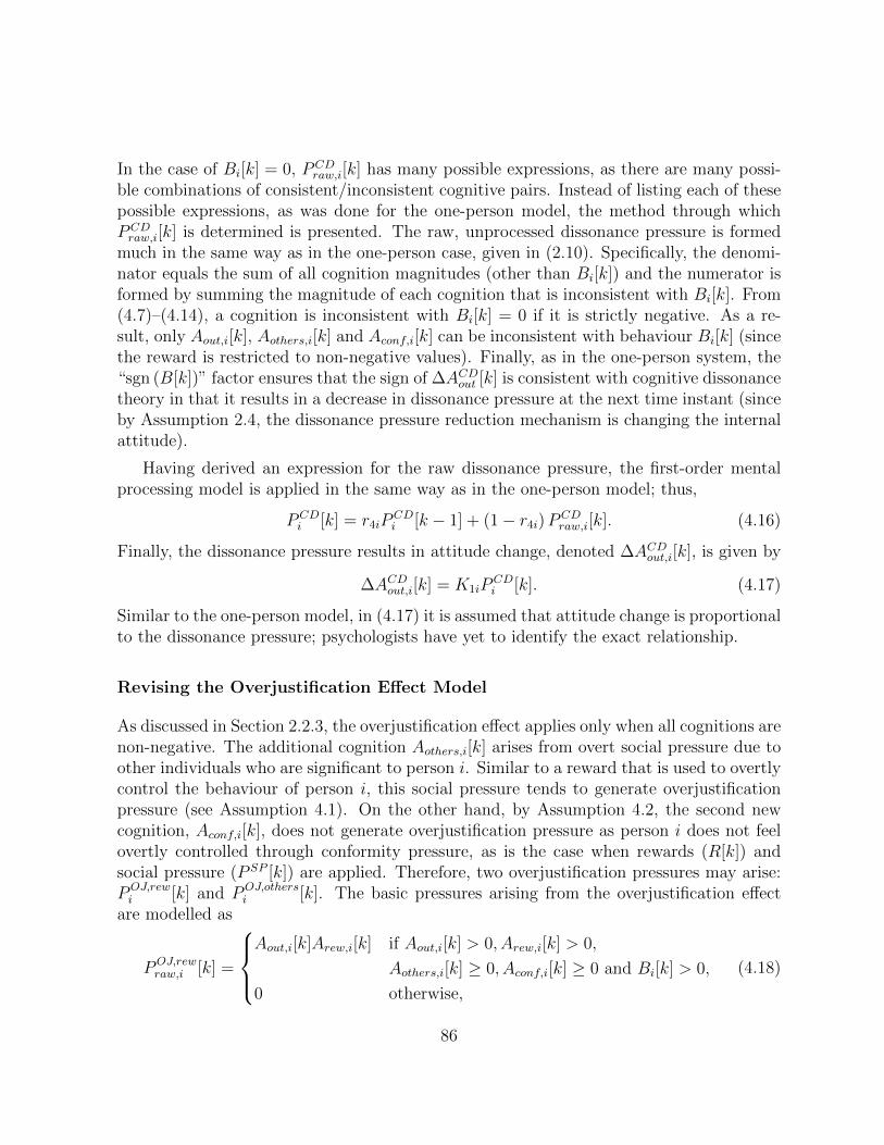
In the case of Bi[k] = 0, PCDraw,i[k] has many possible expressions, as there are many possi-

ble combinations of consistent/inconsistent cognitive pairs. Instead of listing each of thesepossible expressions, as was done for the one-person model, the method through whichPCDraw,i[k] is determined is presented. The raw, unprocessed dissonance pressure is formed

much in the same way as in the one-person case, given in (2.10). Specifically, the denomi-nator equals the sum of all cognition magnitudes (other than Bi[k]) and the numerator isformed by summing the magnitude of each cognition that is inconsistent with Bi[k]. From(4.7)–(4.14), a cognition is inconsistent with Bi[k] = 0 if it is strictly negative. As a re-sult, only Aout,i[k], Aothers,i[k] and Aconf,i[k] can be inconsistent with behaviour Bi[k] (sincethe reward is restricted to non-negative values). Finally, as in the one-person system, the“sgn (B[k])” factor ensures that the sign of ∆ACDout [k] is consistent with cognitive dissonancetheory in that it results in a decrease in dissonance pressure at the next time instant (sinceby Assumption 2.4, the dissonance pressure reduction mechanism is changing the internalattitude).

Having derived an expression for the raw dissonance pressure, the first-order mentalprocessing model is applied in the same way as in the one-person model; thus,

PCDi [k] = r4iP

CDi [k − 1] + (1− r4i)P

CDraw,i[k]. (4.16)

Finally, the dissonance pressure results in attitude change, denoted ∆ACDout,i[k], is given by

∆ACDout,i[k] = K1iPCDi [k]. (4.17)

Similar to the one-person model, in (4.17) it is assumed that attitude change is proportionalto the dissonance pressure; psychologists have yet to identify the exact relationship.

Revising the Overjustification Effect Model

As discussed in Section 2.2.3, the overjustification effect applies only when all cognitions arenon-negative. The additional cognition Aothers,i[k] arises from overt social pressure due toother individuals who are significant to person i. Similar to a reward that is used to overtlycontrol the behaviour of person i, this social pressure tends to generate overjustificationpressure (see Assumption 4.1). On the other hand, by Assumption 4.2, the second newcognition, Aconf,i[k], does not generate overjustification pressure as person i does not feelovertly controlled through conformity pressure, as is the case when rewards (R[k]) andsocial pressure (P SP [k]) are applied. Therefore, two overjustification pressures may arise:POJ,rewi [k] and POJ,others

i [k]. The basic pressures arising from the overjustification effectare modelled as

POJ,rewraw,i [k] =

Aout,i[k]Arew,i[k] if Aout,i[k] > 0, Arew,i[k] > 0,

Aothers,i[k] ≥ 0, Aconf,i[k] ≥ 0 and Bi[k] > 0,

0 otherwise,

(4.18)

86

and

POJ,othersraw,i [k] =

Aout,i[k]Aothers,i[k] if Aout,i[k] > 0, Arew,i[k] ≥ 0,

Aothers,i[k] > 0, Aconf,i[k] ≥ 0 and Bi[k] > 0,

0 otherwise.

(4.19)

Like the one-person system, in (4.18) and (4.19), it is assumed that the pressure dependson the product of the relevant attitudes.

Assuming first-order mental processing of the pressures POJ,rewraw,i [k] and POJ,others

raw,i [k], thefollowing equations for the processed pressures are obtained:

POJ,rewi [k] = r5iP

OJ,rewi [k − 1] + (1− r5i)P

OJ,rewraw,i [k], (4.20)

POJ,othersi [k] = r6iP

OJ,othersi [k − 1] + (1− r6i)P

OJ,othersraw,i [k]. (4.21)

Finally, to avoid the situation where POJ,rewi [k] and POJ,others

i [k] are large enough to actuallychange the sign of Aout,i[k] (an effect that is inconsistent with overjustification theory),

POJ,rewi [k] and POJ,others

i [k] are saturated as follows:

∆AOJ,rewout,i [k] =

−K2iP

OJ,rewi [k] if POJ,rew

i [k] > 0, K2iPOJ,rewi [k] ≤ Aout,i[k],

−Aout,i[k] if POJ,rewi [k] > 0, K2iP

OJ,rewi [k] > Aout,i[k],

0 otherwise,

(4.22)

and

∆AOJ,othersout,i [k] =

−K3iP

OJ,othersi [k] if POJ,others

i [k] > 0, K3i3POJ,othersi [k] ≤ Aout,i[k],

−Aout,i[k] if POJ,othersi [k] > 0, K3iP

OJ,othersi [k] > Aout,i[k],

0 otherwise.

(4.23)Combining these two attitude change equations yields

∆AOJout,i[k] = ∆AOJ,rewout,i [k] + ∆AOJ,othersout,i [k].

Again, like the one-person model, attitude change in (4.22) and (4.23) is assumed to beproportional to the experienced psychological pressure.

4.2.3 Simplifying Assumptions and Initial Conditions

Similar to the one-person system, the problem statement given in Chapter 1 suggests somepreliminary assumptions and initial conditions. The original problem statement considersthe child and his friend. The child’s initial attitude is negative, whereas his friend’s initialattitude is arbitrary. Furthermore, only the child is offered a reward and as a result, thefollowing assumption is made on the reward offered to the friend:

87

Assumption 4.3. Arew,2[k] = 0 for k ≥ 0.

Moreover, the child experiences two external pressures: a reward offered to him by hisparents, and conformity pressure exerted by his friend; thus, this thesis is restricted tothe effects of rewards and conformity pressure (and not any other social pressure) and thefollowing assumption is made:

Assumption 4.4. Aothers,i[k] = 0 for k ≥ 0, i = 1, 2.

Assumption 4.4 simplifies the expression for Bi[k] in (4.5) to

Bi[k] = Aout,i[k] + Arew,i[k] + Aconf,i[k]. (4.24)

In addition, note that from Assumption 4.4 and (4.19), POJ,othersraw,i [k] = 0 for all k ≥ 0

and thus from (4.21), POJ,othersi [k] = 0 for all k ≥ 0. As a result, ∆AOJ,othersout,i [k] = 0 and

consequently the expression for ∆AOJout,i[k] simplifies to

∆AOJout,i[k] = ∆AOJ,rewout,i [k]. (4.25)

Furthermore, previous to sample k = 0, the child and his friend do not experienceany external influences; thus, initially, the behavioural intentions of both the child and hisfriend match their respective initial internal attitudes. Finally, a last reasonable assumptionis that the child and his friend have not previously experienced any pressures due todissonance of overjustification effects and thus, both experience no initial attitude change.Hence, the initial conditions for i = 1, 2 are:

PCDi [0] = POJ

i [0] = 0,

∆ACDout,i[0] = ∆AOJout,i[0] = 0,

Arew,i[0] = Aconf,i[0] = 0,

Bi[0] = Aout,i[0] = Aoi, (4.26)

where Ao1 < 0 and Ao2 is arbitrary. Note that, by Assumption 4.4, the initial conditionson Aothers,1[k] and Aothers,2[k] are omitted.

Finally, similar to the one-person system, assumptions are made on our model’s pa-rameter values as follows:

Assumption 4.5. Gains reflecting how the dissonance and overjustification pressures af-fect attitude change are strictly positive, i.e., K1i > 0, K2i > 0 and K3i > 0.

Assumption 4.6. The value assigned to one dollar is strictly positive, i.e., µ1i > 0.

88

Assumption 4.7. The extent to which each person in the two-person system experiencesconformity pressure cannot be more than 100%, i.e., 0 ≤ µ31 < 1 and 0 ≤ µ32 < 1.

Assumption 4.8. The mental processing pole locations for reward attitude formation andthe conformity attitude formation in (4.2) and (4.4) are zero, i.e., r1i = r3i = 0.

Assumption 4.8 simplifies the expressions for Arew,i[k] and Aconf,i[k] in (4.2) and (4.4)respectively to

Arew,i[k] = µ1iRi[k − 1] (4.27)

Aconf,i[k] = µ3jBj[k − 1]. (4.28)

Assumption 4.9. The mental processing pole locations for dissonance and overjusti-fication pressures in (4.16), (4.20), and (4.21) are contained in the range [0, 1), i.e.,0 ≤ r4i, r5i, r6i < 1.

These assumptions are used throughout the remainder of this chapter, as well as in Chap-ter 5. A final assumption is used only for analysis and does not apply to simulations:

Assumption 4.10. The mental processing pole location for dissonance pressure in (4.16)is zero, i.e., r4i = 0 for i = 1, 2.

Assumption 4.10 simplifies the expressions for PCDi [k] (4.16) to

PCDi [k] = PCD

raw,i[k]. (4.29)

4.3 Model Consistency Verification

The model of Section 4.2 is now verified to be qualitatively consistent with the psychologypresented in Section 4.1. First, the social pressure component is studied by consideringhow it contributes to the theory of planned behaviour, cognitive dissonance theory, andthe overjustification effect. Then, the conformity pressure component of the two-personsystem is examined.

4.3.1 Social Pressure Consistency Verification

We show that the following four qualitative features are exhibited by the social pressurecomponent of the two-person system:

89

1. Strong social pressures have a greater influence on behavioural intent then weak socialpressures.

2. A person tends to reduce dissonance pressure, should it arise.

3. Overjustification pressure, should it arise, cannot cause attitude to switch signs.

4. The magnitude of the attitude change arising from overjustification pressure increaseswith an increase in social pressure and/or attitude towards behavioural outcome.

To perform this qualitative analysis, it is assumed for simplicity that no conformity pressurearises and no reward is offered and thus, the subscript i is omitted from the model equations.

First, a strong social pressure is given by higher magnitudes of P SP [k] in (4.3), leadingto a large Aothers[k] magnitude. From (4.5), large Aothers[k] magnitudes have a greaterinfluence on B[k] than small magnitudes; hence, the model displays the first qualitativecharacteristic listed above.

The second trend, related to dissonance pressure, is the same as in the one-personsystem. Thus, similar to the one-person system, to show dissonance pressure is reducedthrough attitude change, it is sufficient (recalling Assumption 4.10) to show that

|PCDraw [k + 1]| < |PCD

raw [k]|

for any combination of dissonance pressures. Given that Aconf [k] and Arew[k] are as-sumed to be zero for this analysis, there are two cognitive pairs, (Aothers[k], B[k]) and(Aout[k], B[k]); thus, from the two-person model equations, there are four possible situa-tions in which dissonance may arise. These situations are given as follows:

1. Aothers[k] ≥ 0, Aout[k] < 0, B[k] ≥ 0,

2. Aothers[k] ≥ 0, Aout[k] < 0, B[k] < 0,

3. Aothers[k] < 0, Aout[k] ≥ 0, B[k] ≥ 0, and

4. Aothers[k] < 0, Aout[k] ≥ 0, B[k] < 0.

The first two situations are the same as the induced compliance paradigm discussed in theone-person case, with Aothers[k] replacing Arew[k]. As such, the first two situations havealready been shown to satisfy the requirement that |PCD

raw [k + 1]| < |PCDraw [k]|. Now, it only

remains to show that the last two situations satisfy this relationship.

For the situation in which B[k] ≥ 0, from (4.12), Mcon[k] = |Aout[k]B[k]| and from(4.9), Mincon[k] = |Aothers[k]B[k]|. Assuming B[k] 6= 0, from (4.15),

PCDraw [k] =

|Aothers[k]B[k]||Aothers[k]B[k]|+ |Aout[k]B[k]|

=|Aothers[k]|

|Aothers[k]|+ |Aout[k]|. (4.30)

90

Note that if B[k] = 0, then PCDraw [k] = |Aothers[k]|

|Aothers[k]|+|Aout[k]| , which is the same as the above

expression. From (4.16), this raw, unprocessed dissonance pressure produces a positivePCD[k] and thus, from (4.17) and Assumption 4.5, a positive attitude change, i.e.,

Aout[k + 1] = Aout[k] +K1PCD[k] > Aout[k].

Note that ∆AOJout[k] = 0 since the conditions required for overjustification effect to holdare not met. To see how this increased attitude affects the raw, unprocessed dissonancepressure at sample k + 1, assume that the social pressure is constant, ensuring only theeffect of changes to the internal attitude is studied. Since the internal attitude increasesand the social pressure remains constant, B[k] necessarily increases and is, therefore, stillpositive. Hence, from (4.15),

PCDraw [k + 1] =

|Aothers[k + 1]B[k + 1]||Aothers[k + 1]B[k + 1]|+ |Aout[k + 1]B[k + 1]|

=|Aothers[k + 1]|

|Aothers[k + 1]|+ |Aout[k + 1]|

Since Aothers[k + 1] = Aothers[k] and |Aout[k + 1]| > |Aout[k]|, it follows that PCDraw [k + 1] <

PCDraw [k], as required. Note that since PCD

raw [k] > 0, the magnitude signs are omitted.

For the situation in which B[k] < 0, from (4.13), Mcon[k] = |Aothers[k]B[k]| and from(4.8), Mincon[k] = |Aout[k]B[k]|. From (4.15),

PCDraw [k] = − |Aout[k]B[k]|

|Aout[k]B[k]|+ |Aothers[k]B[k]|= − |Aout[k]||Aout[k]|+ |Aothers[k]|

. (4.31)

From (4.16), this raw, unprocessed dissonance pressure produces a negative PCD[k] andthus from (4.17) and Assumption 4.5, a negative attitude change, i.e.,

Aout[k + 1] = Aout[k] +K1PCD[k] < Aout[k].

Similar to before, ∆AOJout[k] = 0. The above attitude effectively decreases B[k] (again,assuming a constant reward attitude); thus B[k+ 1] < 0. Moreover, if this decrease causesAout[k + 1] < 0, then PCD

raw [k + 1] = 0 and thus, dissonance pressure magnitude is reducedvia attitude change. On the other hand, if Aout[k + 1] ≥ 0, then from (4.15),

PCDraw [k + 1] = − |Aout[k + 1]B[k + 1]|

|Aout[k + 1]B[k + 1]|+ |Aothers[k + 1]B[k + 1]|

= − |Aout[k + 1]||Aout[k + 1]|+ |Aothers[k + 1]|

.

Since Aothers[k + 1] = Aothers[k] and Aout[k + 1] < Aout[k], it follows that |PCDraw [k + 1]| <

|PCDraw [k]|, as required. Therefore, in each of the four possible situations in which dissonance

91

pressure arises exclusively from social pressure, attitude change results in a reduction ofthe amount of dissonance pressure experienced.

For illustrative purposes, a simulation is performed for two of the situations in whichdissonance may arise. In both simulations, shown in Figure 4.3, a constant, negative socialpressure is applied to a person in the system, whose initial attitude is positive. Further-more, this person has no reward attitude and no conformity attitude. The simulationresults show the response of the person in question (since no conformity is present). Thefirst simulation, shown in the left plots, is related to the situation in which Aothers[k] < 0,Aout[k] ≥ 0, and B[k] < 0, whereas the second simulation is shown the right plots, andis related to the situation in which Aothers[k] < 0, Aout[k] ≥ 0, and B[k] ≥ 0. As bothsimulations in Figure 4.3 show, when dissonance pressure arises, the raw, unprocessed dis-sonance pressure strength decreases through attitude change. Furthermore, the processeddissonance pressure magnitude, |PCD[k]|, also decreases, as expected. (Since the situationsin which Aothers[k] ≥ 0 and Aout[k] < 0 are essentially the same as the induced complianceparadigm of cognitive dissonance theory, no simulations are given because they would bethe same as those shown in Figure 2.5.) Therefore, the two-person model is consistent withthe second qualitative characteristic on page 90.

The remaining two characteristics, related to the overjustification pressure, are the sameas the overjustification pressure trends in the one-person system. As the equations for theoverjustification pressure arising from social pressure, i.e., POJ

others[k], are the same as thosefor the overjustification pressure arising from rewards, i.e., POJ

rew[k], which has been shownto demonstrate these two trends (see Section 2.4), the two remaining characteristics areindeed exhibited by the two-person system.

4.3.2 Conformity Pressure Consistency Verification

The conformity pressure component of the two-person model is now considered. For thisverification, assume no reward or social pressure is applied. In this case, the two-personmodel is called the zero-input system because no external input is applied to the sys-tem. Recall from Section 4.1.2 that there are two types of conformity, compliance andacceptance. Compliance occurs when a person’s behaviour switches sign due to conformitypressure, while his attitude does not switch sign, whereas acceptance occurs when a personswitches the sign of both his behaviour and attitude; typically behaviour switches first.For our model, showing that it is possible for a person’s behaviour to switch sign due tostrong counter-attitudinal conformity pressure (which refers to the conformity pressure aperson experiences that is contrary to his internal attitude) is evidence that our modelis consistent with at least compliance. Additionally, showing that the sign of the internalattitude can also change is evidence that our model exhibits acceptance. As the acceptancetype of conformity was not explicitly taken into account when modelling the two-person

92

0 10 20 30−100

−50

0

0 10 20 300

100

200

0 10 20 300

0.5

0 10 20 30−100

0

100

200

sample (k)

0 10 20 30−100

−50

0

0 10 20 300

100

200

0 10 20 300

0.5

0 10 20 30−100

0

100

200

sample (k)

Aout[k] Aout[k]

Aothers[k]

B[k]B[k]

|PCDraw[k]| |PCD

raw[k]|

|PCD[k]| |PCD[k]|

Aothers[k]

Figure 4.3: Simulation demonstrating how the two-person system responds to constantsocial pressure. Set Ao = 60 attitude units and consider two social pressure magnitudes:negative social pressure that is strong enough to drive behaviour negative (say, P SP [k] = −2social pressure units, left plots) and negative social pressure that does not cause behaviourto become negative (say, P SP [k] = −1 social pressure units, right plots). The simulationsresults show how Aout[k], Aothers[k], PCD[k] and B[k] respond to the applied social pressure.For the stronger social pressure, Aout[k] decreases. This has the effect of reducing |PCD

raw [k]|and |PCD[k]|. For the weaker social pressure, Aout[k] increases, which has the effect ofreducing PCD

raw [k] and PCD[k]. However, since Aout[k] ≥ 0, B[k] ≥ 0 and Aothers[k] < 0for k ≥ 0, there is always dissonance pressure. It can be shown that this dissonancepressure cannot converge to zero as k tends to infinity; thus Aout[k] (and hence, B[k]) isan unbounded increasing function of k as k tends to infinity.

93

system, showing the model exhibits this effect is of potential interest to psychologists asconformity theory does not traditionally link acceptance with dissonance pressure effects.

To begin, our model is shown to exhibit compliance. From the psychology literature,strong conformity pressure influences an individual’s behaviour more than weak conformitypressure [11]. This trend is exhibited by our model’s theory of planned behaviour equations,specifically, for the zero-input system,

Bi[k] = Aout,i[k] + Aconf,i[k].

Thus, when |Aconf,i[k]| is greater, its effect onBi[k] is also greater. Moreover, ifAout,i[k] < 0,then, provided Aconf,i[k] ≥ 0 and is sufficiently large, it is possible for Bi[k] ≥ 0. In otherwords, a person’s behaviour can become positive due to positive conformity pressure, eventhough his internal attitude is negative. A similar argument holds when Aout,i[k] ≥ 0 andAconf,i[k] < 0. Hence, our model can demonstrate compliance effects.

To show our model can exhibit acceptance, the internal attitude is considered. Inparticular, if conformity pressure forces behaviour to become positive while the internalattitude is negative, then acceptance is demonstrated if the internal attitude also becomes,at some point in time, positive. Similarly, if conformity pressure forces behaviour to be-come negative while the internal attitude is positive, then acceptance is demonstrated ifthe internal attitude also becomes, at some point in time, negative. To determine whetheror not these two trends are exhibited by the two-person system, the effect of a counter-attitudinal conformity pressure on one of the two people in our model is studied. Thisconformity pressure is chosen to be high enough to force the initially consistent cognitivepair, (Aout,i[k], Bi[k]), to become inconsistent, by changing the sign of Bi[k]. If the in-ternal attitude changes according to the above two trends, then we will have shown thatacceptance can be exhibited by our model.

Suppose person one has a negative internal attitude and experiences zero conformitypressure before sample k > 0, i.e., Aconf,1[k] = 0 for 0 ≤ k < k. Then, since Arew,1[k] =Aothers,1[k] = 0 for k ≥ 0, the behaviour of person one, B1[k], equals the internal attitude,Aout,1[k], for 0 ≤ k < k. Both Aout,1[k] and B1[k] remain constant for 0 ≤ k < k sincePCD

1 [k] = 0 and POJ1 [k] = 0 for 0 ≤ k < k, implying ∆Aout,1[k] = 0 over this sample range.

Let Aconf,1[k] > 0 at k = k and suppose this conformity pressure is high enough to causeB1[k] ≥ 0. Then (Aout,1[k], B1[k]) form an inconsistent cognitive pair and, therefore, fromour model’s dissonance pressure equations,

PCDraw,1[k] =

|Aout,1[k]||Aout,1[k]|+ |Aconf,1[k]|

> 0.

Since the raw unprocessed dissonance pressure is positive at k = k and zero for 0 ≤ k < k, itfollows from the model equations that ∆ACDout,1[k] > 0. Moreover, since no overjustification

94

pressure arises, ∆Aout,1[k] = ∆ACDout,1[k] > 0. Therefore,

Aout,1[k + 1] = Aout,1[k] + ∆Aout,1[k] > Aout,1[k].

In other words, person one’s internal attitude increases. If Aout,1[k+1] ≥ 0, then acceptanceoccurs. Otherwise, even though attitude increases, compliance occurs. A similar argumentcan be used to show that if person one has a positive internal attitude and experiencesa sufficiently large, negative conformity pressure, then Aout,1[k] decreases. If the inter-nal attitude decreases to a negative value, then acceptance occurs; otherwise, complianceoccurs.

To summarize, our model is consistent with the psychological trend that conformitypressure influences behaviour. Moreover, a sufficiently large counter-attitudinal confor-mity pressure changes a behaviour’s sign and thus, our model can exhibit compliance. Fi-nally, since this sufficiently large counter-attitudinal conformity pressure produces attitudechange (through our model’s dissonance equations), acceptance may also arise. Therefore,our model is qualitatively consistent with the psychology related to conformity.

Combining the results of this section show that the two-person system is qualitativelyconsistent with the psychology used to develop our model. There are, however, otherpsychological phenomena that arise in a group setting, which were not taken into accountwhen modelling the two-person system. In the next section, these trends are introducedand discussed within the context of our model.

4.4 Other Psychological Phenomena

Psychology researchers who study group dynamics have discovered various phenomenarelated to how people’s attitudes and behaviours change when in a group setting. Threeof these possible trends are relevant to the two-person system and are given below:

1. When all people in a group share a similar attitude, i.e., the sign of each person’sattitude is the same, the average attitude and/or behaviour of the group tends toincrease. This is called group polarization [14].

2. When a person in a group experiences pressure to carry out a behaviour that iscontrary (in sign) to his internal attitude, this person conforms (by complying to thispressure) if his attitude is weak, relative to the average pressure exerted by the group[18].

3. When a person in a group experiences pressure to perform a behaviour that is con-trary (in sign) to his internal attitude, this person reacts (by strengthening the mag-nitude of his pre-existing attitude and/or behaviour) if his attitude is strong, relativeto the average pressure exerted by the group [18].

95

Initial Region Ao1 Ao2 Relationship

I positive positive anyII positive negative |Ao2| ≤ µ31Ao1III positive negative µ31Ao1 < |Ao2| ≤ Ao1

µ32

IV positive negative Ao1µ32

< |Ao2|V negative negative anyVI negative positive Ao2

µ31< |Ao1|

VII negative positive µ32Ao2 < |Ao1| ≤ Ao2µ31

VIII negative positive |Ao1| ≤ µ32Ao2

Table 4.2: Initial operating regions for the two-person system.

The development of the two-person system modelled the immediate impact conformitypressure has on the behaviour of an individual and did not attempt to model the threetrends described above; thus, showing the two-person system is qualitatively consistentwith these trends is of potential interest to psychologists and to us, since it provides fur-ther evidence of the validity of our model. Most interesting, perhaps, is the consistency ofthe model with the reactance trend above, as in this situation, dissonance pressure arisesand is the mechanism through which this trend is exhibited. To the best of our knowledge,psychologists have not explicitly linked the reactance trend with cognitive dissonance the-ory, but our model suggests that dissonance theory may be a possible explanation for thischaracteristic.

The three psychological trends above depend on a person’s internal attitude, and itsstrength, relative to the average conformity pressure exerted by the group. For our model,there are two people, and therefore, there is no need to average the conformity pressureexperienced by each person. To determine which of the three psychological trends a personin our model will exhibit, the relative strength of each initial attitude is examined (becauseeach initial attitude produces a conformity pressure at k = 1). Table 4.2 defines eightpossible relationships between the two initial attitudes. These eight relationships formeight initial operating regions, shown graphically in Figure 4.4. If the zero-input systembegins in regions I or V, then both people share a similar (i.e., same sign) attitude and,therefore, psychology predicts that group polarization should occur. If the system beginsin region II, IV, VI or VIII, then the two people do not share a similar attitude and oneattitude is relatively weak, while the other is relatively strong; thus, psychology predictsthat the person with the weak attitude should conform and the person with the strongattitude should react. Finally, if the system begins in region III or VII, then the twopeople do not share a similar attitude, and neither attitude is weak (or strong) relativeto the other. In this case, psychology does not predict whether reactance or conformity

96

Ao1

Ao2

I

II

IIIIV

V

VI

VII

VIII

Figure 4.4: Graphical representation of initial operating regions of the two-person system.Regions are denoted on the graph and lines are given by the relationships in Table 4.2.

should occur (only that each person should exhibit one of these two trends). Table 4.3summarizes these expected psychological trends for each initial region given in Table 4.2.Note that because each person’s attitude may change over time, the relative strength ofeach person’s attitude may also change, in which case, the expected psychological trendmay change. As a result, Table 4.3 summarizes the short-term expected psychological trendfor the zero-input system. Showing that our model demonstrates the three group dynamictrends above (group polarization, reactance, conformity) amounts to showing the zero-input system response of each initial region is consistent with the relevant psychologicaltrend given in Table 4.3. This analysis is carried out in Chapter 5 due to its relevance tocontroller design.

To summarize, this chapter relaxes the assumption that an individual experiences onlyone external influence (a reward) and considers the effect a second person has on theattitude and behaviour of the first individual. Two general types of external influenceswere explained, social pressure and conformity pressure. Then, a two-person discrete-timemodel was developed using the framework of the one-person model and the new psychologypresented in this chapter. The two-person system was shown to be qualitative consistencywith the psychology related to social pressure and conformity pressure. Finally, otherpsychological phenomena arising from group dynamics were introduced. Verification ofthe consistency between the zero-input system and these phenomena is given in Chapter 5,along with open-loop and closed-loop controller design.

97

Initial Region Expected PsychologicalTrend for Person One

Expected PsychologicalTrend for Person Two

I Group Polarization Group PolarizationII Reactance ConformityIII Conformity or Reactance Reactance or ConformityIV Conformity ReactanceV Group Polarization Group PolarizationVI Reactance ConformityVII Conformity or Reactance Reactance or ConformityVIII Conformity Reactance

Table 4.3: Short-term psychological trends expected for each initial region of the two-personsystem.

98

Chapter 5

Two-Person System:Simulation and Control Strategies

This chapter explores open-loop and closed-loop control strategies to achieve a controlobjective for the two-person system with the initial conditions given in (4.26): the controlobjective is to determine whether or not, for any Bd > 0, there exists a reward sequence,R1[k], such that B1[k] ≥ Bd as k tends to infinity. For this analysis, the assumptionspresented in Section 4.2.3 are used.

In the last section of Chapter 4, three psychological phenomena related to group dynam-ics were introduced: group polarization, conformity and reactance. To determine whetheror not these trends are exhibited by the two-person system, the zero-input response of eachof the eight initial operating regions (see Figure 4.4) is determined. This chapter beginswith this analysis. Key qualitative characteristics uncovered in this analysis are then ex-ploited to design controllers that meet the control objective. First, open-loop controllersare considered; then, due to drawbacks of open-loop control, closed-loop controllers aredesigned to meet the required control objective.

5.1 Zero-Input Response Analysis

Table 5.1 collects together various responses of the zero-input system, labelled A1–D1.Each of these responses characterizes at least one of the three psychological phenomenaarising from group dynamics, as indicated in Table 5.1. By comparing the zero-inputresponse for each initial region with the response descriptions in Table 5.1, the psychologicaltrend(s) arising for each initial region can be determined. In some initial regions, thesystem exhibits different psychological trends over time, i.e., the short-term psychological

99

trends exhibited by some initial regions are different than the long-term trends. For eachinitial region, if the short-term psychological trends exhibited by the model’s zero-inputresponse are consistent with the expected psychological trends, as given in Table 4.3, thenthe model is qualitatively consistent with the trends predicted by psychology related togroup dynamics.

For this analysis, regions V, VI, VII and VIII are considered since, from the initialconditions, Ao1 is restricted to negative values. From Table 4.2, initial regions I, II, IIIand IV correspond with non-negative values for Ao1. Even though these four regions arenot included in the analysis, the initial regions are symmetric about the Ao1 = −Ao2 axis(see Figure 4.4). Furthermore, each person in the two-person system is modelled by thesame set of equations. As such, the zero-input system response is symmetric about theAo1 = −Ao2 axis, meaning the responses of initial regions I, II, III and IV can be inferredfrom those of initial regions V, VI, VII and VIII. Finally, in some cases, an approximationis made for |µn31µ

m32| for any whole numbers m and n with m + n ≥ 2. Specifically, since

|µ31| < 1 and |µ32| < 1 (by Assumption 4.7), their product is also less than one. Forsome of this analysis, this product is approximated as |µn31µ

m32| ≈ 0 for any m and n with

m+ n ≥ 2.

5.1.1 Zero-Input Response Analysis: Region V

First, suppose the system begins in region V, which is defined by the following initialattitude relationship:

Ao1, Ao2 < 0. (5.1)

From the system’s initial conditions given in (4.26), B1[0] = Ao1 and B2[0] = Ao2; thus,both behaviours are also initially negative. As a result, each person experiences negativeconformity pressure, further decreasing their behaviour at k = 1. Each person’s behaviourat k = 1 is still consistent with their attitude at k = 1 because for i = 1, 2, Aout,i[1] =Aout,i[0] + ∆Aout,i[0] and, from (4.26), ∆Aout,i[0] = 0 for i = 1, 2, meaning Aout,i[1] =Aoi < 0. Moreover, since each person experiences negative conformity pressure at k = 1,the cognitive pair (Aconf,i[1], Bi[1]) is also consistent, implying dissonance pressure does notarise at k = 1. Finally, by Assumption 4.2 and the fact that the zero-input system assumesArew,i[k] = 0 for k ≥ 0, i = 1, 2, overjustification pressure cannot arise, i.e., POJ,rew

i [k] = 0for k ≥ 0, i = 1, 2; consequently, ∆Aout,i[1] = 0 for i = 1, 2. This argument can be repeatedfor each k ≥ 0, leading to the following conclusion:

Lemma 5.1. For the zero-input two-person system with the initial conditions given by(4.26), if the initial attitudes satisfy (5.1), then, for k ≥ 0, and i = 1, 2,

(a) ∆ACDout,i[k] = 0 and

100

Resp

onse

Desc

rip

tion

Psy

cholo

gic

al

Tre

nd

for

Pers

on

One

Psy

cholo

gic

al

Tre

nd

for

Pers

on

Tw

o

A1

Fork≥k,Aout,

1[k

],Aout,

2[k

],B

1[k

],B

2[k

]≥

0.B

1[k

],B

2[k

]ar

ein

crea

sing

funct

ions

ofk

and

sett

leto

stea

dy-s

tate

valu

es.

Gro

up

Pol

ariz

atio

nG

roup

Pol

ariz

atio

n

A2

Fork≥k,Aout,

1[k

],B

1[k

],B

2[k

]≥

0,Aout,

2[k

]<

0.B

1[k

],B

2[k

]ar

ein

crea

sing

funct

ions

ofk

and

sett

leto

stea

dy-s

tate

valu

es.

Rea

ctan

ceC

onfo

rmit

y

A3

Fork≥k,Aout,

2[k

],B

1[k

],B

2[k

]≥

0,Aout,

1[k

]<

0.B

1[k

],B

2[k

]ar

ein

crea

sing

funct

ions

ofk

and

sett

leto

stea

dy-s

tate

valu

es.

Con

form

ity

Rea

ctan

ce

B1

Fork≥k,Aout,

1[k

],B

1[k

]≥

0,Aout,

2[k

],B

2[k

]<

0.B

1[k

]in

crea

ses

and

isunb

ounded

andB

2[k

]dec

reas

esan

dis

unb

ounded

.

Rea

ctan

ceR

eact

ance

C1

Fork≥k,Aout,

1[k

],Aout,

2[k

],B

1[k

],B

2[k

]<

0.B

1[k

],B

2[k

]ar

edec

reas

ing

funct

ions

ofk

and

sett

leto

stea

dy-s

tate

valu

es.

Gro

up

Pol

ariz

atio

nG

roup

Pol

ariz

atio

n

C2

Fork≥k,Aout,

1[k

],B

1[k

],B

2[k

]<

0,Aout,

2[k

]≥

0.B

1[k

],B

2[k

]ar

edec

reas

ing

funct

ions

ofk

and

sett

leto

stea

dy-s

tate

valu

es.

Rea

ctan

ceC

onfo

rmit

y

C3

Fork≥k,Aout,

2[k

],B

1[k

],B

2[k

]<

0,Aout,

1[k

]≥

0.B

1[k

],B

2[k

]ar

edec

reas

ing

funct

ions

ofk

and

sett

leto

stea

dy-s

tate

valu

es.

Con

form

ity

Rea

ctan

ce

D1

Fork≥k,Aout,

2[k

],B

2[k

]≥

0,Aout,

1[k

],B

1[k

]<

0.B

2[k

]in

crea

ses

and

isunb

ounded

andB

1[k

]dec

reas

esan

dis

unb

ounded

.

Rea

ctan

ceR

eact

ance

Tab

le5.

1:D

escr

ipti

onof

two-

per

son

syst

emre

spon

ses

and

the

rela

ted

psy

chol

ogic

altr

ends.

101

(b) ∆AOJout,i[k] = 0.

Proof. See Appendix E.1.

Lemma 5.1 dictates that if the zero-input, two-person system begins in region V, thenboth attitudes remain constant for k ≥ 0. (Moreover, a similar argument holds if the systembegins in region I.) In the case when both people in the zero-input system experienceno dissonance or overjustification pressures, the expressions for B1[k] and B2[k] can besimplified:

Lemma 5.2. For the zero-input two-person system with the initial conditions given by(4.26), if for k ≥ 0 and i = 1, 2

(i) ∆ACDout,i[k] = 0, and

(ii) ∆AOJout,i[k] = 0,

then, for k ≥ 1,

B1[k] = Ao1

(1− (µ31µ32)1+b k

2c

1− (µ31µ32)

)+ µ32Ao2

(1− (µ31µ32)1+b k−1

2c

1− (µ31µ32)

)(5.2)

B2[k] = µ31Ao1

(1− (µ31µ32)1+b k−1

2c

1− (µ31µ32)

)+ Ao2

(1− (µ31µ32)1+b k

2c

1− (µ31µ32)

). (5.3)


By Lemma 5.1, if the system begins in region V, then the conditions of Lemma 5.2 apply;therefore, the above lemma provides simplified expressions for B1[k] and B2[k] when thesystem begins in region V. From these expressions, the system response is determined.

Along with Assumption 4.7, (5.2) and (5.3) imply that the zero-input response of initialregion V is stable in the sense that B1[k] and B2[k] converge and all other signals remainbounded as k tends to infinity. Moreover, Assumption 4.7, (5.2) and (5.3) imply thatB1[k] < 0 and B2[k] < 0 for k ≥ 0. Not only are both behaviours negative for all k ≥ 0, itcan be shown that they are decreasing functions of k for k ≥ 0:

Lemma 5.3. For the zero-input two-person system with the initial conditions given by(4.26), if the initial attitudes satisfy (5.1), then

(a) Aout,1[k] < 0, Aout,2[k] < 0, B1[k] < 0, B2[k] < 0, for all k ≥ 0, and

102

0 2 4 6 8 10 12 14 16 18 20

−40

−30

−20

0 2 4 6 8 10 12 14 16 18 20−40

−20

0

0 2 4 6 8 10 12 14 16 18 20−80

−60

−40

−20

sample (k)

Aout,2[k]

Aconf,1[k]

Aconf,2[k]

B1[k]B2[k]

Aout,1[k]

Figure 5.1: Simulation results of the two-person system, with the initial conditions givenin (4.26), parameter values in Table 4.1, beginning in region V with no reward applied tothe system. Person one’s initial attitude is Ao1 = −40 attitude units, whereas person two’sinitial attitude is Ao2 = −25 attitude units. The simulation results confirm Lemma 5.3since all attitudes and behaviours remain negative for k ≥ 0, while both behaviours aredecreasing functions of k for k ≥ 0, eventually converging to steady-state values.

(b) B1[k] and B2[k] are decreasing functions of k, converging as k tends to infinity.


The system response given by Lemma 5.3 is the same as that described by responsetype C1 in Table 5.1, where k = 0; consequently, if the system begins in initial regionV, then its response is of type C1 (both in the short-term and in the long-term). FromTable 5.1, response type C1 characterizes group polarization for person one and persontwo. This is consistent with the prediction given by Table 4.3, which indicates that if thesystem begins in region V, then the short-term psychological trend it should exhibit is thegroup polarization phenomenon. To illustrate the trends of Lemma 5.3, simulation resultsare shown in Figure 5.1.

103

5.1.2 Zero-Input Response Analysis: Region VI

Now, suppose the system begins in region VI, which is defined by the following conditionson the two initial attitudes:

Ao1 < 0, Ao2 ≥ 0,

Ao2 < µ31|Ao1|. (5.4)

Unlike in the case of initial region V, for initial region VI dissonance pressure may ariseand, thus, the expressions for B1[k] and B2[k] in Lemma 5.2 are not applicable. Instead,more general equations are needed. Iterating through the system equations yields

B1[k] =

Ao1 if k = 0

B1[0] + µ32Ao2 if k = 1,

B1[1] +K11PCD1 [1] + µ31µ32Ao1 if k = 2,

B1[k − 1] +K11PCD1 [k − 1]+

µ32

b k−12c∑

i=1

K12PCD2 [k − 2i] (µ31µ32)i−1 if k ≥ 3,

+∑b k−2

2c

i=1 K11PCD1 [k − 2i− 1]µi31µ

i−132 + µ

b k−22c+1

31 µb k−1

2c

32 Aoi

](5.5)

B2[k] =

Ao2 if k = 0

B2[0] + µ31Ao1 if k = 1,

B2[1] +K12PCD2 [1] + µ31µ32Ao2 if k = 2,

B2[k − 1] +K12PCD2 [k − 1]+

µ31

b k−12c∑

i=1

K11PCD1 [k − 2i] (µ31µ32)i−1 if k ≥ 3,

+∑b k−2

2c

i=1 K12PCD2 [k − 2i− 1]µi32µ

i−131 + µ

b k−22c+1

32 µb k−1

2c

31 Aoj

](5.6)

where {j = 1, i = 2, if k is odd

j = 2, i = 1 if k is even.

Along with Assumption 4.10 and the approximation that |µn31µm32| ≈ 0 for any m and n with

m+n ≥ 2, these two equations can be used to deduce the signs of B1[k] and B2[k] for k ≥ 0.Once the signs of B1[k] and B2[k] are known for k ≥ 0, the signs of PCD

1 [k] and PCD2 [k]

are easily obtained from Assumption 4.10. Specifically, if Bi[k] < 0 then PCDi [k] ≤ 0;

104

otherwise PCDi [k] ≥ 0. (It is possible for there to be zero dissonance pressure at some

sample and, thus, this possibility is included.) By Assumption 4.2, dissonance pressureis the only pressure driving attitude change and, therefore, the sign of Bi[k] indicates theattitude change direction of Aout,i[k].

When the system begins in region VI, the initial attitude of person one is strong relativeto person two and, therefore, the conformity pressure of person one should dominate. Inother words, the behaviour of person one is strong enough such that it should drive persontwo’s behaviour negative. From (5.5) and (5.6), it can be shown that this is the case. Infact, not only does person two’s behaviour eventually become negative due to the negativeconformity pressure exerted by person one, it becomes negative at k = 1 and remainsnegative for k ≥ 1. Additionally, person one’s behaviour remains negative for k ≥ 0. Thelemma below formalizes this conclusion.

Lemma 5.4. For the zero-input two-person system with the initial conditions given by(4.26), if the initial attitudes satisfy (5.4), and the approximation |µn31µ

m32| ≈ 0 for any m

and n with m+ n ≥ 2 is used, then for k ≥ 1

B1[k] < 0

B2[k] < 0.


The above lemma states that if the system begins in region VI, then both behavioursare negative for k ≥ 1, implying (from the previous discussion) that Aout,i[k] is a non-increasing function of k for k ≥ 1 and i = 1, 2. For Aout,1[k], this conclusion guarantees theattitude of person one remains negative for k ≥ 0. For Aout,2[k], this conclusion means thatthe attitude of person two may become negative at some sample, k∗, or by Lemma A.1,converge to some non-negative constant as k tends to infinity.

Although Lemma 5.4 says that both behaviours remain negative for k ≥ 1, moreinformation about the response of these two signals can be obtained by considering (5.5)and (5.6). In particular, from (5.5) and the approximation on |µn31µ

m32|, B1[k] can be

approximated as

B1[k] ≈ B1[k − 1] +K11PCD1 [k − 1] + µ32K12P

CD2 [k − 2].

for k ≥ 3. From Lemma 5.4, for k ≥ 3, B1[k − 1] < 0 and B2[k − 2] < 0, thus from (4.29)PCD

1 [k − 1] < 0 and PCD2 [k − 2] < 0. As a result, B1[k] < B1[k − 1] for k ≥ 3. Similarly,

B2[k] < B2[k−1] for k ≥ 3. Combining these two conclusions implies that for k ≥ 3, B1[k]and B2[k] are decreasing functions of k. Not only are these two signals decreasing functionsof k, it can also be shown that each converges as k tends to infinity. The following lemmasummarizes the response of the two-person system beginning in region VI.

105



and n with m+ n ≥ 2 is used, then

(a) Aout,1[k] < 0, B1[k] < 0 and B2[k] < 0, for k ≥ 1,

(b) Aout,2[k] ≥ 0 for k ≥ 0, or there exists a k∗ such that Aout,2[k] ≥ 0 for 0 ≤ k < k∗ andAout,2[k] < 0 for all k ≥ k∗, and

(c) B1[k] and B2[k] are non-increasing functions of k for k ≥ 3, converging as k tends toinfinity.


The system response given by Lemma 5.5 is the same as that described by responsetypes C1 and C2 in Table 5.1. The case when Aout,2[k] ≥ 0 for k ≥ 0 corresponds with

response type C2, where k = 3, whereas the case when Aout,2[k] < 0 for k ≥ k∗ corresponds

with response type C1 where k = k∗. From Table 5.1, response type C2 characterizes reac-tance for person one and conformity for person two. This is consistent with the predictiongiven in Table 4.3, which indicates that if the system begins in region VI, then it shouldexhibit reactance for person one and conformity for person two. Additionally, althoughresponse type C1, which corresponds to group polarization, does not match the expectedpsychological trend give in Table 4.3, recall that Table 4.3 gives the short-term expectedpsychological trends for each initial region. In the case when Aout,2[k] < 0 for k ≥ k∗,it’s also true that Aout,2[k] ≥ 0 for 0 ≤ k < k∗, and therefore, over this range, personone exhibits reactance and person two exhibits conformity, which is consistent with theprediction given in Table 4.3. To illustrate the trends of Lemma 5.5, simulation results areshown in Figure 5.2.

5.1.3 Zero-Input Response Analysis: Region VIII

Before continuing to initial region VII, initial region VIII is considered. This region isdefined by the following initial attitudes:

Ao1 < 0, Ao2 ≥ 0,

|Ao1| ≤ µ32Ao2. (5.7)

The initial signs of Ao1 and Ao2 are the same as those of region VI. Furthermore, the aboverelationship between the two attitudes is symmetric (across the Ao1 = −Ao2 axis) withtheir relationship in region VI, given by (5.4). This similarity between the initial attitude

106

0 2 4 6 8 10 12 14 16 18 20−50

0

50

0 2 4 6 8 10 12 14 16 18 20−40

−20

0

20

0 2 4 6 8 10 12 14 16 18 20−100

−50

0

50

sample (k)

Aout,1[k]

Aout,2[k]

Aconf,1[k]Aconf,2[k]

B2[k] B1[k]

Figure 5.2: Simulation results of the two-person system, with the initial conditions givenin (4.26), parameter values in Table 4.1, beginning in region VI with no reward appliedto the system. Person one’s initial attitude is Ao1 = −40 attitude units, whereas persontwo’s initial attitude is Ao2 = 15 attitude units, thus satisfying the relationship given in(5.4). This simulation confirms Lemmas 5.4 and 5.5 since both behaviours are negative,decreasing functions of k for k ≥ 1, converging as k →∞, while Aout,1[k] < 0 for k ≥ 0. Inthe above simulation, Aout,2[k] becomes negative at k = 4, resulting in response type C1

where k = 4.

107

relationships of regions VI and VIII suggests a symmetry in their responses. Since, ininitial region VI, the attitude of person one is strong relative to person two, person twoconforms to the behaviour of person one. On the other hand, in initial region VIII, theattitude of person two is strong relative to person one and thus by symmetry, personone should conform to the behaviour of person two and therefore their behaviour shouldbecome positive, suggesting a type A response. From Table 5.1, apart from the attitudeand behaviour signs, response type A1 is identical to response type C1. Similarly, responsetype A3 is symmetric (across the Ao1 = −Ao2 axis) with type C2. Consequently, thefollowing lemma describes the system response when the initial attitudes are in regionVIII, which is symmetric with the zero-input system response of initial region VI, given inLemma 5.5.




(a) Aout,2[k] ≥ 0, B1[k] ≥ 0 and B2[k] ≥ 0, for k ≥ 1,

(b) Aout,1[k] < 0 for k ≥ 0, or there exists a k∗ such that Aout,1[k] < 0 for 0 ≤ k < k∗ andAout,1[k] ≥ 0 for all k ≥ k∗, and

(c) B1[k] and B2[k] are increasing functions of k for k ≥ 3, converging as k tends toinfinity.

Proof. The lemma follows from Lemma 5.5 and symmetry with region VI.

Similar to Lemma 5.5, Lemma 5.6 is also the same as two responses described in Ta-ble 5.1. In particular, the case when Aout,1[k] < 0 for k ≥ 0 corresponds with response type

A3, where k = 3, while the case when Aout,1[k] ≥ 0 for k ≥ k∗ corresponds with response

type A1, where k = k∗. As before, Table 5.1 indicates the psychological phenomenonexhibited by each response type. Using the same arguments as initial region VI, the re-sponse of the zero-input system beginning in region VIII can be shown to be consistentwith the short-term expected psychological trends given in Table 4.3. To illustrate thetrends of Lemma 5.6, simulation results are shown in Figure 5.3. These simulation resultsalso illustrate further the point that the system responses of initial regions VI and VIIIare symmetric.

5.1.4 Zero-Input Response Analysis: Region VII

Finally, the response of the system beginning in region VII is studied. This region is themost complicated and, perhaps, the most interesting region to study, as very different types

108

0 2 4 6 8 10 12 14 16 18 20−50

0

50

0 2 4 6 8 10 12 14 16 18 20−20

0

20

40

0 2 4 6 8 10 12 14 16 18 20−50

0

50

100

sample (k)

Aout,2[k]

Aconf,1[k]

B2[k]B1[k]

Aconf,2[k]

Aout,1[k]

Figure 5.3: Simulation results of the two-person system, with the initial conditions given in(4.26), parameter values in Table 4.1, beginning in region VIII with no reward applied tothe system. Person one’s initial attitude is Ao1 = −15 attitude units, whereas person two’sinitial attitude is Ao2 = 40 attitude units, thus satisfying the relationship given in (5.7).The initial conditions used for this simulation are symmetric with those of the simulationfor region VI. The magnitudes of person one’s signals in this simulation are the same asthe magnitudes of the corresponding signals of person two in the simulation results givenin Figure 5.2, while their sign is different (and vice versa for person two). Therefore,this simulation also provide evidence supporting the argument that the zero-input systemresponse is symmetric across the Ao1 = −Ao2 axis. Moreover, this simulation confirmsLemma 5.6 since both behaviours and Aout,2[k] are positive for k ≥ 1. At k = 4, Aout,1[k]

becomes positive, resulting in response type A1 where k = 4.

109

of system response can occur. In this region, the two attitudes have approximately thesame strength, but differ in sign. Psychology literature suggests that in this case, peoplecan either react or conform. If one person conforms, then the other person likely reacts.However, as will be demonstrated in this subsection, our model predicts that it is alsopossible for both people to react, with both people’s attitudes and behaviours becomingstronger.

For initial region VII, defined by the following initial attitudes,

Ao1 < 0, Ao2 ≥ 0,

µ32Ao2 < |Ao1| ≤Ao2µ31

, (5.8)

the behaviour can be expressed by (5.5) and (5.6). From the above relationship between theinitial attitudes, it can be shown (from (5.5) and (5.6)) that for 0 ≤ k ≤ 2, B1[k] < 0 andB2[k] ≥ 0. From (4.29), negative dissonance pressure arises from a negative behaviour, andpositive dissonance pressure arises from a positive behaviour. By Assumption 4.2, attitudechange is driven only by dissonance pressure and, therefore, for 0 ≤ k ≤ 2, Aout,1[k] is adecreasing function of k, whereas Aout,2[k] is an increasing function of k. At this point, thesystem response depends on the relative size of K11 and K12; thus three possible situationsarise for k = 3:

1. K11 and K12 are similar enough to ensure B1[3] < 0 and B2[3] ≥ 0;

2. K11 is small relative to K12 and therefore, B1[3] ≥ 0 and B2[3] ≥ 0; and

3. K12 is small relative to K11 and therefore, B1[3] < 0 and B2[3] < 0.

For the last two of these three situations, it is possible to show that after k = 3, eachbehaviour signal maintains its sign for k ≥ 3, as summarized in the lemma below.




(a) if B1[3] ≥ 0 and B2[3] ≥ 0, then for k ≥ 3, B1[k] ≥ 0 and B2[k] ≥ 0; whereas

(b) if B1[3] < 0 and B2[3] < 0, then for k ≥ 3, B1[k] < 0 and B2[k] < 0.


110

Lemma 5.7 gives two possible responses for the behaviour signals. The analysis for thesituation in which B1[3] < 0 and B2[3] ≥ 0 is more complicated, yet simulations suggestthat in this case, B1[k] < 0 and B2[k] ≥ 0 for k ≥ 3. This detail is presented after analysingthe two above known system responses.

First, consider the case when B1[k] ≥ 0 and B2[k] ≥ 0 for k ≥ 3. Since Ao2 ≥ 0 andB2[k] ≥ 0 for k ≥ 0, from (4.29), PCD

2 [k] ≥ 0 for k ≥ 0; thus, for k ≥ 0, Aout,2[k] ≥ 0 and isa non-decreasing function of k. Moreover, since B1[k] ≥ 0 for k ≥ 3, PCD

1 [k] ≥ 0 for k ≥ 3.If, for all k ≥ 3, Aout,1[k] < 0, then PCD

1 [k] > 0, otherwise, all cognitions are positiveand no dissonance pressure arises; hence, either Aout,1[k] is an increasing function of k fork ≥ 3, remaining negative (thus converging) as k tends to infinity, or Aout,1[k] becomespositive at some sample k = k∗ and remains positive for k ≥ k∗. This response is the sameas that described by Lemma 5.6, which corresponds with initial region VIII. Therefore, ifB1[3] ≥ 0 and B2[3] ≥ 0, the system response is similar to that of initial region VIII, asgiven in the lemma below.

Lemma 5.8. For the zero-input two-person system with the initial conditions given by(4.26), if the initial attitudes satisfy (5.8), B1[3] ≥ 0, B2[3] ≥ 0, and the approximation|µn31µ

m32| ≈ 0 for any m and n with m+ n ≥ 2 is used, then

(a) B1[k] ≥ 0, B2[k] ≥ 0 and Aout,2[k] ≥ 0 for k ≥ 3;

(b) Aout,1[k] < 0 for k ≥ 0, or there exists some k∗ such that Aout,1[k] < 0 for 0 ≤ k < k∗

and Aout,1[k] ≥ 0 for k ≥ k∗; and

(c) B1[k] and B2[k] converge as k →∞.


Similar to Lemma 5.6, the system response given by Lemma 5.8 is the same as thatdescribed by response types A1 and A3 in Table 5.1. It can be argued (as before) thatresponse given by Lemma 5.8 is consistent with the short-term expected psychologicaltrends given in Table 4.3. To illustrate the trends of Lemma 5.8, simulation results areshown in Figure 5.4.

Now consider the second result of Lemma 5.7, where B1[k] < 0 and B2[k] < 0 for k ≥ 3.By symmetry across the Ao1 = −Ao2 axis, the previous argument can be used to show thatthe system response is given by the following lemma.

Lemma 5.9. For the zero-input two-person system with the initial conditions given by(4.26), if the initial attitudes satisfy (5.8), B1[3] < 0, B2[3] < 0, and the approximation|µn31µ


111

0 2 4 6 8 10 12 14 16 18 20−20

0

20

40

0 2 4 6 8 10 12 14 16 18 20−50

0

50

0 2 4 6 8 10 12 14 16 18 20−50

0

50

sample (k)

Aout,2[k]

Aconf,2[k]

Aconf,1[k]

B2[k]B1[k]

Aout,1[k]

Figure 5.4: Simulation results of the two-person system, with the initial conditions given in(4.26) beginning in region VII with no reward applied to the system. With the exceptionof µ32 and K11, parameter values used are those given in Table 4.1. Person one’s initialattitude is Ao1 = −10 attitude units, whereas person two’s initial attitude is Ao2 = 10.5attitude units. Moreover, µ32 = 0.95, thus the relationship given in (5.8) is satisfied.Finally, K11 = 5 (thus K11 is small relative to K12 = 30). At k = 3, both behaviours arepositive and remain positive for k ≥ 3, thus confirming Lemma 5.7. Finally, the simulationresults show both attitudes are non-decreasing functions of k for k ≥ 3 and both behavioursconverge as k tends to infinity, which supports the results of Lemma 5.8. Due to Aout,1[k]

remaining negative for all k ≥ 0, the system response is of type A3 where k = 3.

112

0 2 4 6 8 10 12 14 16 18 20−40

−20

0

20

0 2 4 6 8 10 12 14 16 18 20−50

0

50

0 2 4 6 8 10 12 14 16 18 20−50

0

50

sample (k)

B2[k]

Aout,2[k] Aout,1[k]

Aconf,1[k]

Aconf,2[k]

B1[k]

Figure 5.5: Simulation results of the two-person system, with the initial conditions givenin (4.26) beginning in region VII with no reward or social pressure applied to the system.With the exception of µ31 and K12, parameter values used are those given in Table 4.1.Person one’s initial attitude is Ao1 = −10.5 attitude units, whereas person two’s initialattitude is Ao2 = 10 attitude units. Moreover, µ31 = 0.95, thus the relationship given in(5.8) is satisfied. Finally, K12 = 5. At k = 3, both behaviours are negative and therefore,the simulation results confirm Lemma 5.7, as both behaviours remain negative for k ≥ 3.Finally, the simulation results support Lemma 5.9 because they show that both attitudesare decreasing functions of k and both behaviours converge as k tends to infinity. Due toAout,2[k] remaining positive for all k ≥ 0, the system response is of type C2 where k = 3.

(a) B1[k] < 0, B2[k] < 0 and Aout,1[k] < 0 for k ≥ 3;

(b) Aout,2[k] ≥ 0 for k ≥ 0, or there exists some k∗ such that Aout,2[k] ≥ 0 for 0 ≤ k < k∗

and Aout,2[k] < 0 for k ≥ k∗; and

(c) B1[k] and B2[k] converge as k →∞.

Proof. The lemma follows from symmetry with Lemma 5.8.

The system response given by Lemma 5.9 is the same as that described by responsetypes C1 and C2 in Table 5.1. It can be argued (as before) that response given byLemma 5.9 is consistent with the short-term expected psychological trends given in Ta-ble 4.3. The simulation results given in Figure 5.5 illustrate the results of Lemma 5.9 and,again, highlight the symmetric trend exhibited by the system.

113

Finally, the situation in which B1[3] < 0 and B2[3] ≥ 0 is discussed. Simulationssuggest that when this situation arises, B1[k] < 0 and B2[k] ≥ 0 for k ≥ 3. Suppose itis true that B1[3] < 0 and B2[3] ≥ 0 implies B1[k] < 0 and B2[k] ≥ 0 for k ≥ 3; then,both people experience dissonance pressure due to the conformity pressure exerted by theother individual. From (4.29), these dissonance pressures cause Aout,1[k] to decrease andAout,2[k] to increase. Since Aout,1[k] is initially negative and is a decreasing function of k,it follows that it remains negative. Likewise, Aout,2[k] ≥ 0 for k ≥ 0. Since dissonancepressure always exists for each person, neither attitude converges as k tends to infinity andas a result Aout,1[k] → −∞ and Aout,2[k] → ∞ as k → ∞ and, hence, neither behaviourconverges. Therefore, the conjecture below is presented to summarize the observed systembehaviour in this situation.

Conjecture 5.1. For the zero-input two-person system with the initial conditions given by(4.26), if the initial attitudes satisfy (5.8), B1[3] < 0, B2[3] ≥ 0, and the approximation|µn31µ


(a) B1[k] < 0 and B2[k] ≥ 0 for k ≥ 0;

(b) Aout,1[k] < 0 and Aout,2[k] ≥ 0 for k ≥ 0; and

(c) B1[k]→ −∞ and B2[k]→∞ as k →∞.

The system response given in the above conjecture is the same as that described byresponse type D1 in Table 5.1. Interesting to note is that both people exhibit reactance,since the attitude and behaviour of each person maintains its original sign and becomesstronger as k tends to infinity. The simulation shown in Figure 5.6 provides evidencesupporting the results of Conjecture 5.1.

The results of the initial region VII analysis are interesting because they confirm thatboth reactance and compliance may arise when conformity pressure is experienced. Theseresults are consistent with psychology literature related to conformity, as are the possi-ble responses of initial regions V, VI and VIII. Although, when developing our model,the dynamic effects of conformity were not considered, it is interesting that our systemexhibits these trends through dissonance pressure. This result suggests that cognitive dis-sonance may be a key underlying mechanism that is responsible for the trends discoveredby psychologists.

5.2 Open-Loop Investigation

To begin investigating whether or not there exists a reward sequence, R1[k], 0 ≤ k < ∞,such that B1[k] ≥ Bd as k → ∞, an open-loop control strategy is first studied. The

114

0 2 4 6 8 10 12 14 16 18 20−200

0

200

0 2 4 6 8 10 12 14 16 18 20−50

0

50

0 2 4 6 8 10 12 14 16 18 20−100

0

100

sample (k)

Aout,2[k]

Aconf,1[k]

Aout,1[k]

Aconf,2[k]

B1[k]

B2[k]

Figure 5.6: Simulation results of the two-person system, with the initial conditions givenin (4.26), parameter values in Table 4.1, beginning in region VII with no reward applied tothe system. Person one’s initial attitude is Ao1 = −10 attitude units, whereas person two’sinitial attitude is Ao2 = 10.5 attitude units, thus satisfying the relationship given in (5.8).This simulation provides evidence to support Conjecture 5.1, because B1[3] < 0, B2[3] ≥ 0,and all attitudes and behaviours maintain their initial signs for k → ∞. Moreover, thebehaviours tend to positive/negative infinity as k tends to infinity, resulting in responsetype D1 for k ≥ 0.

115

dynamics of the two-person system are more complicated than the one-person system asdemonstrated by the analysis in the last section. Nevertheless, the one-person open-loopinvestigation in Section 3.1 provides some insight into where the two-person open-loopinvestigation could begin. The first open-loop control strategy considered for the one-person system was an impulse reward, which was shown to not necessarily be able to meetthe control objective. As the two-person system contains the dynamics of the one-personsystem, and additional dynamics due to the conformity feedback loop, the impulse-rewardcontrol strategy is not even considered in this analysis. Instead, motivated by the successof the step-reward control strategy presented in Section 3.1.2, a step reward is examinedhere. Since person one is the only person being offered a reward, the reward sequence,R1[k], is the control signal, and is simply denoted R[k] (see Figure 4.1).

Applying a step reward to the two-person system means that the child’s parents offerhim a fixed amount of money each day, with the hope that the child eventually producesthe desired behavioural intent, denoted here by some Bd > 0. Moreover, this child andhis friend influence each other’s behaviour through conformity pressure. The problem isto determine whether or not there exists some Ro > 0 and control signal

R[k] = Ro, k ≥ 0 (5.9)

such that B1[k] ≥ Bd as k tends to infinity. From (4.27) this control signal generates areward attitude signal for k ≥ 1 given by

Arew,1[k] = µ1Ro. (5.10)

Before proceeding with the analysis to find an Ro that meets the control objective, aneasier problem is studied. Since the control objective is to drive B1[k] ≥ Bd as k tendsto infinity, it is useful to know whether or not it is possible to at least drive person one’sbehaviour positive. Instead of finding an Ro that drives B1[k] ≥ 0 as k → ∞, the resultsof the zero-input analysis motivate finding an Ro that drives B1[k] ≥ 0 for k ≥ 1. Inparticular, the zero-input analysis from the previous section demonstrates that the mostcomplicated dynamics occur within the first few samples, when the signs of B1[k] and B2[k]are switching. Knowing the signs of B1[k] and B2[k] is one of the more useful pieces ofinformation for understanding the system’s response. By driving B1[k] ≥ 0 immediately,the analysis is simplified, as the reward’s effect on the first few samples of each behaviourcan be considered explicitly, and then, through induction, its effect on the remainingsamples of each behaviour can be determined. Thus, the easier problem of finding an Ro

such that B1[k] ≥ 0 for k ≥ 1 is studied, providing useful tools for solving the main controlobjective.

116

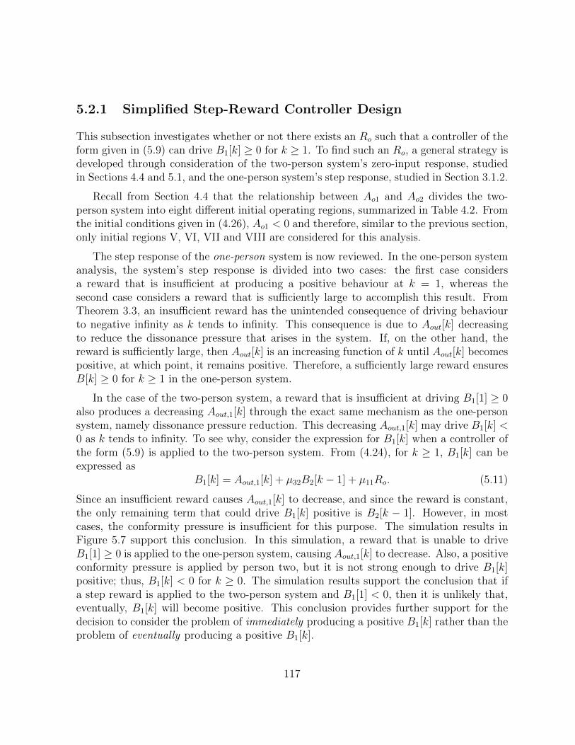
5.2.1 Simplified Step-Reward Controller Design

This subsection investigates whether or not there exists an Ro such that a controller of theform given in (5.9) can drive B1[k] ≥ 0 for k ≥ 1. To find such an Ro, a general strategy isdeveloped through consideration of the two-person system’s zero-input response, studiedin Sections 4.4 and 5.1, and the one-person system’s step response, studied in Section 3.1.2.

Recall from Section 4.4 that the relationship between Ao1 and Ao2 divides the two-person system into eight different initial operating regions, summarized in Table 4.2. Fromthe initial conditions given in (4.26), Ao1 < 0 and therefore, similar to the previous section,only initial regions V, VI, VII and VIII are considered for this analysis.

The step response of the one-person system is now reviewed. In the one-person systemanalysis, the system’s step response is divided into two cases: the first case considersa reward that is insufficient at producing a positive behaviour at k = 1, whereas thesecond case considers a reward that is sufficiently large to accomplish this result. FromTheorem 3.3, an insufficient reward has the unintended consequence of driving behaviourto negative infinity as k tends to infinity. This consequence is due to Aout[k] decreasingto reduce the dissonance pressure that arises in the system. If, on the other hand, thereward is sufficiently large, then Aout[k] is an increasing function of k until Aout[k] becomespositive, at which point, it remains positive. Therefore, a sufficiently large reward ensuresB[k] ≥ 0 for k ≥ 1 in the one-person system.

In the case of the two-person system, a reward that is insufficient at driving B1[1] ≥ 0also produces a decreasing Aout,1[k] through the exact same mechanism as the one-personsystem, namely dissonance pressure reduction. This decreasing Aout,1[k] may drive B1[k] <0 as k tends to infinity. To see why, consider the expression for B1[k] when a controller ofthe form (5.9) is applied to the two-person system. From (4.24), for k ≥ 1, B1[k] can beexpressed as

B1[k] = Aout,1[k] + µ32B2[k − 1] + µ11Ro. (5.11)

Since an insufficient reward causes Aout,1[k] to decrease, and since the reward is constant,the only remaining term that could drive B1[k] positive is B2[k − 1]. However, in mostcases, the conformity pressure is insufficient for this purpose. The simulation results inFigure 5.7 support this conclusion. In this simulation, a reward that is unable to driveB1[1] ≥ 0 is applied to the one-person system, causing Aout,1[k] to decrease. Also, a positiveconformity pressure is applied by person two, but it is not strong enough to drive B1[k]positive; thus, B1[k] < 0 for k ≥ 0. The simulation results support the conclusion that ifa step reward is applied to the two-person system and B1[1] < 0, then it is unlikely that,eventually, B1[k] will become positive. This conclusion provides further support for thedecision to consider the problem of immediately producing a positive B1[k] rather than theproblem of eventually producing a positive B1[k].

117

0 2 4 6 8 10 12 14 16 18 20−2

0

2

4

0 2 4 6 8 10 12 14 16 18 20−2

0

2

4

0 2 4 6 8 10 12 14 16 18 20−200

0

200

0 2 4 6 8 10 12 14 16 18 20−50

0

50

0 2 4 6 8 10 12 14 16 18 20−100

0

100

sample (k)

R1[k]

Arew,1[k] Arew,2[k]

B1[k]

B2[k]

Aconf,2[k]

Aconf,1[k]

Aout,1[k]

Aout,2[k]

R2[k]

Figure 5.7: A controller of the form (5.9) is applied to the two-person system with theinitial conditions given in (4.26), parameter values in Table 4.1, where Ao1 = −10 attitudeunits, Ao2 = 12 attitude units and Ro = $3. This reward is insufficient at driving B1[1] ≥ 0and, therefore, Aout,1[k] decreases. Even though the conformity pressure exerted on personone is positive, i.e., Aconf,1[k] ≥ 0, it is not sufficient to overcome the decreasing Aout,1[k],and, as a result, B1[k] < 0 for k ≥ 0.

118

On the other hand, if the reward causes B1[1] ≥ 0, then Aout,1[k] increases. Shouldthis increase cause Aout,1[k] ≥ 0, overjustification pressure may arise (due to the reward),causing Aout,1[k] (and thus B1[k]) to decrease. However, similar to the one-person system,overjustification pressure is able to decrease Aout,1[k] only to a certain point: it is not ableto drive Aout,1[k] < 0, as summarized in the lemma below.

Lemma 5.10. If, for the two-person system, there is a k such that

(i) Arew,1[k] ≥ 0,

(ii) Aout,1[k] ≥ 0, and

(iii) Aconf,1[k] ≥ 0 for k ≥ k,

then for k ≥ k, Aout,1[k] is a non-increasing function of k, lower bounded by zero.


The above lemma implies that if Aout,1[k] decreases due to overjustification pressure, thena sufficiently large reward can be applied to counteract any negative effect this decreasinginternal attitude has on B1[k].

Although a reward that drives B1[1] ≥ 0 causes Aout,1[k] to initially increase, theadditional dynamics of B2[k] may be such that B2[k] (and thus, Aconf,1[k]) is a decreasingfunction that causes B1[k] to become negative. To see why, consider the expression forB2[k], which, from (4.24), is given by

B2[k] = Aout,2[k] + µ31B1[k − 1]. (5.12)

If B2[k] < 0, then any dissonance pressure that arises causes Aout,2[k] to decrease. ShouldB2[k] remain negative, Aout,2[k] remains a decreasing function of k and thus, it is possiblethat Aconf,1[k], through B2[k], becomes strong enough to drive B1[k] < 0 (see (5.11)).On the other hand, if B2[k] is positive, then any dissonance pressure that arises causesAout,2[k] to increase and thus, increases B2[k] (and, through Aconf,1[k], B1[k]). Therefore,it is desirable to also drive B2[k] positive. The reward first affects B2[k] at k = 2. Asbefore, if B2[2] < 0, then B2[k] is unlikely to become positive due to a decreasing Aout,2[k].Thus, the control strategy also attempts to drive B2[2] ≥ 0.

To summarize, the approach for achieving the easier control objective is to find an Ro

such that when a controller of the form (5.9) is applied to the two-person system, B1[1] ≥ 0and B2[2] ≥ 0. Since B1[1] and B2[2] are given by

B1[1] = Ao1 + µ32Ao2 + µ11Ro (5.13)

B2[2] = Ao2 +K12PCD2 [1] + µ31 (Ao1 + µ11Ro + µ32Ao2) , (5.14)

119

such an Ro must satisfy the following two inequalities:

Ro ≥ −Ao1 + µ32Ao2

µ11

and (5.15)

Ro ≥ −Ao2 (1 + µ31µ32) +K12P

CD2 [1] + µ31Ao1

µ31µ11

. (5.16)

Although these two inequalities drive B1[1] ≥ 0 and B2[2] ≥ 0, they do not necessarilyimply that B1[k] ≥ 0 for k ≥ 1, due to the complicated dynamics arising from the con-formity feedback loop. However, by slightly modifying the conditions given in (5.15) and(5.16), not only can we guarantee B1[k] ≥ 0 for k ≥ 1, but also B2[k] ≥ 0 for k ≥ 2.Modifications to (5.15) and (5.16) are specific to the sign of PCD

2 [1], which depends on theinitial operating region. If the system begins in region V, VII or VIII, then PCD

2 [1] ≥ 0,whereas PCD

2 [1] < 0 if the system begins in region VI. These two cases are consideredseparately, beginning with initial regions V, VII and VIII .

Suppose the system begins in region V. Then, since B2[1] is given by B2[1] = Ao2 +µ31Ao1, both cognitions at k = 1 are negative and thus, PCD

2 [1] = 0. On the other hand, ifthe system begins in region VII, then Ao2 > 0 and Ao2 ≥ µ31|Ao1|. As a result, B2[1] ≥ 0and thus from (4.29), PCD

2 [1] > 0. Finally, if the system begins in region VIII, then Ao2 > 0

and Ao2 ≥ |Ao1|µ32

. As a result, B2[1] ≥ 0 and thus from (4.29), PCD2 [1] > 0. From (5.14), if

PCD2 [1] ≥ 0, then ensuring

Ao2 + µ31 (Ao1 + µ11Ro + µ32Ao2) ≥ 0

is sufficient to guarantee B2[2] ≥ 0. By rearranging the above inequality, the range ofsufficient Ro values able to drive B2[2] ≥ 0 is given by

Ro ≥ −Ao2 (1 + µ31µ32) + µ31Ao1

µ11µ31

. (5.17)

Thus, for initial regions V, VII and VIII, driving B1[1] ≥ 0 and B2[2] ≥ 0 requires thatboth (5.15) and (5.17) hold. The reward magnitude that satisfies these two inequalitiescan be refined to guarantee B1[k] ≥ 0 for k ≥ 1 and B2[k] ≥ 0 for k ≥ 2. The lemmabelow presents the refined Ro that satisfies the given strategy of driving both behaviourspositive.

Lemma 5.11. If a control signal of the form (5.9) is applied to the two-person system withthe initial conditions given by (4.26), and the initial attitudes satisfy (5.1), (5.7) or (5.8),then B1[k] ≥ 0 for k ≥ 1 and B2[k] ≥ 0 for k ≥ 2 when

Ro ≥ max

{−Ao1 (1 + µ31µ32) + µ32Ao2

µ11

,−(Ao2 + µ31Ao1) (1 + µ31µ32)

µ11µ31

}. (5.18)

120


The second expression in (5.18) is the same as the right-hand side of (5.17) with anadditional term, µ2

31µ32Ao1, which is used to guarantee B1[k] ≥ 0 for k ≥ 1 and B2[k] ≥0 for k ≥ 2. To demonstrate the effectiveness of the above controller, a simulation isperformed, shown in the left-hand side plots of Figure 5.8. The plots on the right-handside of Figure 5.8 show that the control strategy given in Lemma 5.11 is conservative.

Now, suppose the system begins in region VI. Then, since Ao2 ≥ 0 and Ao2 < µ31|Ao1|,it follows that B2[1] < 0 and, thus, dissonance pressure arises due to the inconsistencybetween B2[1] and Aout,2[1] = Ao2. From (4.29), this dissonance pressure is given by

PCD2 [1] = − |Ao2|

|Ao2|+ µ31|Ao1|.

As a result, (5.16) can be expressed as

Ro ≥1

µ11µ31

(K12|Ao2|

|Ao2|+ µ31|Ao1|− (Ao2 (1 + µ31µ32) + µ31Ao1)

). (5.19)

For initial region VI, ensuring B1[1] ≥ 0 and B2[2] ≥ 0 requires that both (5.15) and(5.19) hold. The reward magnitude that satisfies these two inequalities can be refined toguarantee B1[k] ≥ 0 for k ≥ 1 and B2[k] ≥ 0 for k ≥ 2. The lemma below presents therefined Ro that satisfies the given strategy of driving both behaviours positive.

Lemma 5.12. If a control signal of the form (5.9) is applied to the two-person system withthe initial conditions given by (4.26), and the initial attitudes satisfy (5.4), then B1[k] ≥ 0for k ≥ 1 and B2[k] ≥ 0 for k ≥ 2 when

Ro ≥ max

{−Ao1 (1 + µ31µ32) + µ32Ao2

µ11

,

1

µ11µ31

(K12Ao2

Ao2 + µ31|Ao1|− (Ao2 + µ31Ao1) (1 + µ31µ32)

)}. (5.20)


The second expression in (5.20) is the same as (5.19) with an additional term, µ231µ32Ao1,

which is used to guarantee B1[k] ≥ 0 for k ≥ 1 and B2[k] ≥ 0 for k ≥ 2. To demonstratethe effectiveness of the above controller, a simulation is performed, shown in the left plotsof Figure 5.9. The plots on the right-hand side of Figure 5.9 show that the control strategygiven in Lemma 5.12 is conservative.

121

0 5 10 15 200

20

40

60

0 5 10 15 200

20

40

60

0 5 10 15 20

−100

0

100

0 5 10 15 20−50

0

50

0 5 10 15 20−100

0

100

sample (k)

0 5 10 15 200

20

40

60

0 5 10 15 200

20

40

60

0 5 10 15 20

−100

0

100

0 5 10 15 20−50

0

50

0 5 10 15 20−100

0

100

sample (k)

Arew,1[k]

R1[k]

R2[k]

R1[k]

R2[k]

Arew,1[k]

Arew,2[k] Arew,2[k]

Aout,1[k]

Aout,2[k]Aout,1[k]

Aout,2[k]

Aconf,1[k] Aconf,2[k] Aconf,1[k]

Aconf,2[k]

B1[k]B2[k]B1[k] B2[k]

Figure 5.8: A controller of the form (5.9) is applied to the two-person system with the initialconditions given in (4.26), parameter values in Table 4.1, where Ao1 = −10 attitude unitsand Ao2 = −20 attitude units (thus the system begins in initial region V). The plots onthe left-hand side show the simulation results for a reward magnitude that satisfies (5.18),specifically, Ro = $63. This reward is sufficient to drive B1[1] ≥ 0 and B2[2] ≥ 0 and tokeep both behaviours positive for k ≥ 2. The plots on the right-hand side demonstratethat not only is Lemma 5.11 conservative because the reward magnitude, Ro = $60, doesnot satisfy (5.18), but the strategy of driving B1[k] ≥ 0 for k ≥ 1 and B2[k] ≥ 0 for k ≥ 2 isalso conservative, since in this simulation B2[k] < 0 as k tends to infinity yet B1[k] ≥ 0 fork ≥ 1. Initial region V is used for simulations to show that even in the case when personone experiences significant, negative conformity pressure, it is possible to drive B1[k] ≥ 0as k tends to infinity.

122

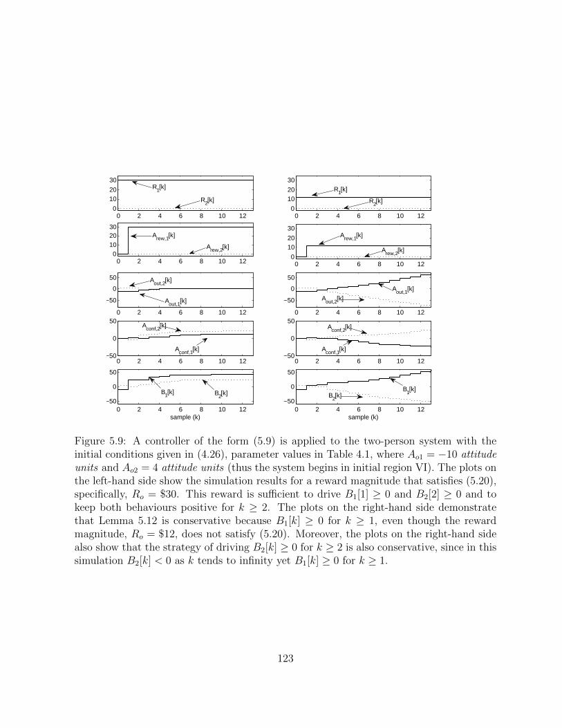
0 2 4 6 8 10 120

1020

30

0 2 4 6 8 10 120

102030

0 2 4 6 8 10 12

−50

0

50

0 2 4 6 8 10 12−50

0

50

0 2 4 6 8 10 12−50

0

50

sample (k)

0 2 4 6 8 10 120

1020

30

0 2 4 6 8 10 120

1020

30

0 2 4 6 8 10 12

−50

0

50

0 2 4 6 8 10 12−50

0

50

0 2 4 6 8 10 12−50

0

50

sample (k)

R1[k]

B1[k] B1[k]

Arew,2[k]

R2[k]

B2[k] B2[k]

Aconf,1[k]

Aconf,2[k]

Aconf,1[k]

Aconf,2[k]

Aout,2[k]

Aout,2[k]

Aout,1[k]

Arew,2[k]

R2[k]

R1[k]

Arew,1[k]Arew,1[k]

Aout,1[k]

Figure 5.9: A controller of the form (5.9) is applied to the two-person system with theinitial conditions given in (4.26), parameter values in Table 4.1, where Ao1 = −10 attitudeunits and Ao2 = 4 attitude units (thus the system begins in initial region VI). The plots onthe left-hand side show the simulation results for a reward magnitude that satisfies (5.20),specifically, Ro = $30. This reward is sufficient to drive B1[1] ≥ 0 and B2[2] ≥ 0 and tokeep both behaviours positive for k ≥ 2. The plots on the right-hand side demonstratethat Lemma 5.12 is conservative because B1[k] ≥ 0 for k ≥ 1, even though the rewardmagnitude, Ro = $12, does not satisfy (5.20). Moreover, the plots on the right-hand sidealso show that the strategy of driving B2[k] ≥ 0 for k ≥ 2 is also conservative, since in thissimulation B2[k] < 0 as k tends to infinity yet B1[k] ≥ 0 for k ≥ 1.

123

To conclude this section, Lemmas 5.11 and 5.12 provide sufficient conditions on Ro

such that for k ≥ 1, B1[k] ≥ 0. This goal is achieved by finding an Ro that is able todrive the behaviour of both people positive for k ≥ 2. These two lemmas show that,provided the reward is high enough, not only are parents able to induce their child toplay the piano when he does not want to, this reward is also enough to entice the child’sfriend to play the piano as well, even though the friend is not being offered a reward. Thisresult is somewhat interesting and highlights the impact conformity pressure may have onan individual’s behaviour. The conclusions of this section suggest that, provided a highenough reward is offered, parents can eventually induce their child to to play piano atsome desired strength, Bd > 0; thus, in the next section, the main control objective isconsidered.

5.2.2 General Step-Reward Controller Design

This section investigates whether or not, for all Bd > 0, there exists an Ro such that acontroller of the form given in (5.9) can drive B1[k] ≥ Bd as k →∞. The strategy to findsuch an Ro builds on the results of the previous section. To obtain a closed-form expressionfor a sufficient reward to meet the control objective, first it is shown that it is possible forB1[k] to converge as k tends to infinity. Then, the expression for B1[∞] can be used tofind a reward that is sufficient to drive B1[k] ≥ Bd as k tends to infinity.

Before determining whether or not an Ro exists such that B1[k] converges as k tendsto infinity, a few preliminary results are needed. Since B1[k] depends on Aout,1[k] andAout,2[k] (indirectly through Aconf,1[k]), it is necessary to characterize Aout,1[k] and Aout,2[k]as k tends to infinity. From Lemmas 5.11 and 5.12, it is possible to drive B1[k] ≥ 0 fork ≥ 1 and B2[k] ≥ 0 for k ≥ 2. When both behaviours are positive, by Assumption 4.10,both attitudes are non-decreasing functions of k until Aout,1[k] becomes positive (at whichtime, Aout,1[k] decreases due to the overjustification effect). Similar to Lemma 3.3 fromthe one-person system, if both behaviours are positive, then each attitude converges as ktends to infinity. The lemma below formalizes this result.

Lemma 5.13. For the two-person system with the initial conditions given by (4.26), ifB1[k] ≥ 0 for k ≥ 1 and B2[k] ≥ 0 for k ≥ 2, then Aout,1[k] and Aout,2[k] converge to someconstants c1 and c2 respectively as k tends to infinity. Moreover,

(a) if there exists some k > 0 such that Aout,1[k] > 0, then c1 = 0, otherwise, c1 ≤ 0; and

(b) if there exists some k > 2 such that Aout,2[k] > 0, then c2 = Aout,2[k], otherwise, c2 ≤ 0.


124

The above lemma states that if a reward drives B1[k] ≥ 0 for k ≥ 1 and B2[k] ≥ 0 fork ≥ 2, then both attitudes converge as k tends to infinity. For Aout,2[k], the condition thatk > 2 (instead of k > 0) is a technical detail that accounts for the case when PCD

2 [1] < 0,and the delay between when the reward is first applied and the sample at which it firstaffects person two.

Since both attitudes converge as k tends to infinity, each attitude is bounded. Thisconclusion is promising because B1[k] and B2[k] depend on both attitudes, i.e.,

B1[k] = Aout,1[k] + µ11Ro + µ32Aout,2[k − 1] + µ31µ32B1[k − 1]

B2[k] = Aout,2[k] + µ31Aout,1[k − 1] + µ31µ11Ro + µ31µ32B2[k − 1]

In both of the above equations, the only signals that could possibly be unbounded areB1[k] and B2[k]. Through a non-trivial analysis, Assumption 4.7 and Lemma 5.13 can beused to show that both behaviours are bounded. The lemma below formalizes this result.

Lemma 5.14. If a control signal of the form (5.9) is applied to the two-person systemwith the initial conditions given by (4.26) and drives B1[k] ≥ 0 for k ≥ 1 and B2[k] ≥ 0for k ≥ 2, then B1[·] and B2[·] are bounded.


At this point, it has been shown that there exists an Ro such that a controller of theform given by (5.9) is able to drive B1[k] ≥ 0 for k ≥ 1 and B2[k] ≥ 0 for k ≥ 2 and thesetwo behaviours are bounded. To show that, in this situation, B1[k] converges as k tendsto infinity, consider that by defining

α[k] := Aout,1[k] + µ1Ro + µ32Aout,2[k − 1],

B1[k] can be expressed as

B1[k] = α[k] + µ31µ32B1[k − 2]. (5.21)

From Lemma 5.13, α[k] is bounded, and, from Lemma 5.14, B1[k] is bounded. If it can beshown that for large enough k, α[k] is a non-decreasing function of k, then, since B1[k] isbounded and is given by (5.21), it follows (from Lemma A.2) that B1[k] must necessarilyconverge as k tends to infinity. Since α[k] depends on Aout,1[k] and Aout,2[k], showing α[k]is eventually a non-decreasing function of k requires knowing more information about thesteady-state values of Aout,1[k] and Aout,2[k].

From Lemma 5.13, if Aout,1[k] becomes positive, then Aout,1[k] necessarily tends to zeroas k tends to infinity. To determine the value to which Aout,1[k] converges in the case whenAout,1[k] < 0 for k ≥ 0, the dissonance pressure expression is considered. It turns out thatsince B2[k] is a bounded function of k, again Aout,1[k] necessarily converges to zero, asstated in the lemma below.

125

Lemma 5.15. If a control signal of the form (5.9) is applied to the two-person systemwith the initial conditions given by (4.26) and drives B1[k] ≥ 0 for k ≥ 1 and B2[k] ≥ 0for k ≥ 2, then

Aout,1[k]→ 0 as k →∞.


Now, consider Aout,2[k], which, from Lemma 5.13, converges as k tends to infinity.Since, by Lemma 5.13, the steady-state value of Aout,2[k] is given in the case when Aout,2[k]becomes positive at some k > 2, it only remains to determine the value for Aout,2[∞] in thecase when Aout,2[k] < 0 for k ≥ 2. Similar to Aout,1[k], the dissonance pressure expressionand the results Lemma 5.14 imply that Aout,2[k] tends to zero as k tends to infinity. Thelemma below formalizes these conclusions.


(a) if, at some k > 2, Aout,2[k] ≥ 0, then Aout,2[k]→ Aout,2[k] as k →∞;

(b) otherwise, Aout,2[k]→ 0 as k →∞.


Now, the results of Lemmas 5.15 and 5.16 can be used to show that for large enough k,α[k] in (5.21) remains non-negative, implying that B1[k] converges as k tends to infinity.The steady-state value of B1[k] is given by the lemma below.


limk→∞

B1[k] =µ11Ro + µ32c2

1− µ31µ32

. (5.22)


In other words, the above lemma demonstrates that there exists an Ro such that whenstep reward is applied to the two-person system, B1[k] converges as k tends to infinity,provided this Ro is sufficient to drive both behaviours positive for k ≥ 2. From Lemmas5.11 and 5.12, there exists an Ro that is able to meet this condition. Such an Ro mustsatisfy (5.18) if the system begins in regions V, VII or VIII, or (5.20) if the system begins

126

in region VI. Define R1o as the reward magnitude at the right-hand side of (5.18) and R2

o

as the reward magnitude at the right-hand side of (5.20). Now, it only remains to find anexpression for an Ro that is able to drive B1[k] ≥ Bd as k tends to infinity. This amountsto setting, by (5.22),

µ11Ro + µ32c2

1− µ31µ32

≥ Bd,

and rearranging for Ro, giving the following inequality:

Ro ≥Bd (1− µ31µ32)− µ32c2

µ11

. (5.23)

With the exception of c2, all of the terms in the above inequality are given directly by theparameter values. From Lemma 5.16, c2 has two possible values: zero (in the case whenAout,2[k] remains negative) and Aout,2[k] (in the case when Aout,2[k] becomes positive). From(5.23), a lower bound on c2 provides a value that can replace c2 in the above inequality.Of the two possible steady-state values for Aout,2[k], zero is the smallest. Thus, if

Ro ≥Bd (1− µ31µ32)

µ11

, (5.24)

then (5.23) also holds. If the system begins in region V, VII or VIII, then, providedRo ≥ R1

o, the above inequality ensures B1[k] ≥ Bd as k tends to infinity. Similarly, ifthe system begins in region VI, then, provided Ro ≥ R2

o, the above inequality ensuresthe control objective is met. Define R3

o as the reward magnitude at the right-hand sideof (5.24). By combining the results of Lemmas 5.11, 5.12 and 5.17, the final theorem isobtained, which gives an expression for a sufficient Ro such that a step-reward controlleris able to meet the control objective of driving B1[k] ≥ Bd as k tends to infinity.

Theorem 5.1. For all Bd > 0, if a control signal of the form (5.9) is applied to thetwo-person system with the initial conditions given by (4.26), then, provided

Ro ≥

{max {R1

o, R3o} if (5.1), (5.7) or (5.8) hold,

max {R2o, R

3o} if (5.4) holds,

(5.25)

B1[k] ≥ Bd as k tends to infinity.


The above theorem states that a step reward is able to meet the control objective of drivingB1[k] ≥ Bd as k tends to infinity. Instead of selecting the maximum value between R1

o, R2o

and R3o, two cases are considered: the first case considers the situation in which PCD

2 [1] ≥ 0,while the second case considers the situation in which PCD

2 [1] < 0. By distinguishing

127

between these two situations, the reward most specific to the initial conditions can beobtained. In particular, R2

o, which is specific to initial region VI, compensates for theeffect of negative dissonance pressure experienced by person two at k = 1. If the systembegins in region V, then no dissonance pressure arises (for either person) at k = 1; thus R2

o

is higher than the value necessary to meet the control objective when the system beginsin region V. Practically speaking, suppose, in the piano example, that the child and hisfriend both have initially negative attitudes. If the child’s parents offer a reward that is atleast the maximum value between R1

o, R2o and R3

o, then these parents are spending moremoney than is required for convincing their child to play the piano at some desired level.Instead, the parents can save money by offering the maximum value between R1

o and R3o,

as proposed by (5.25).

A second interesting consequence of Theorem 5.1 is that in some cases, the reward valuenecessary to drive B1[k] ≥ 0 and B2[k] ≥ 0 for k ≥ 2, i.e., R1

o or R2o, is greater than R3

o.This is typically the case for highly negative initial attitudes, as the reward must overcometheir negative effect on B1[k] and B2[k]. In these situations, B1[k] settles to a steady-statevalue that is greater than Bd. The simulation results given in Figure 5.10 demonstratethis consequence along with the results of Theorem 5.1. A simulation is performed for twosituations, both of which begin in region V. The plots on the left-hand side show the resultsof a simulation for attitudes that, relative to the desired behaviour, are weak; thus, theRo = R3

o. The plots on the right-hand side show the results of a simulation for attitudesthat are strong enough to require Ro = R1

o. In this situation, B1[k] converges to a valuegreater than Bd as k tends to infinity.

The strategy of driving B1[k] ≥ 0 for k ≥ 1 and B2[k] ≥ 0 for k ≥ 2 proves to be auseful stepping-stone for achieving the main control objective, as many key results arisefrom this strategy. These key results include determining B1[k] and B2[k] are bounded(Lemma 5.14), obtaining steady-state expressions for Aout,1[k] and Aout,2[k] (Lemmas 5.15and 5.16), and finding a steady-state expression for B1[k] (Lemma 5.17), from which arange of Ro values that are able to meet the control objective is obtained. However, eventhough Theorem 5.1 states that is it possible to meet the control objective with a stepreward, open-loop control has drawbacks and, therefore, a closed-loop control approach isconsidered.

5.3 Closed-Loop Investigation

Similar to the controller design for the one-person system, closed-loop control is consid-ered because of its general benefits (i.e., the ability to more effectively fight disturbancesand uncertainty). For the one-person system, two types of closed-loop controllers weredesigned: state-feedback and output-feedback. Since the output-feedback controller design

128

0 10 20 30 40 500

20

4060

0 10 20 30 40 500

204060

0 10 20 30 40 50−20

−10

0

10

0 10 20 30 40 50

0

20

40

0 10 20 30 40 50

0

50

100

sample (k)

0 10 20 30 40 500

20

4060

0 10 20 30 40 500

20

4060

0 10 20 30 40 50−20

−10

0

10

0 10 20 30 40 50

0

20

40

0 10 20 30 40 50

0

50

100

sample (k)

B2[k]B1[k]


Aout,2[k]Aout,1[k]

Arew,2[k]

Arew,1[k]

R1[k] R2[k]R1[k]

R2[k]

Arew,1[k]

Arew,2[k]

Aout,1[k] Aout,2[k]


B1[k]B2[k]

Figure 5.10: A controller of the form (5.9) is applied to the two-person system with theinitial conditions given in (4.26), parameter values in Table 4.1 and Bd = 75 attitude units.The plots on the left-hand side show a situation in which Ao1 = −10 attitude units andAo2 = −5 attitude units. In this situation, the attitude magnitudes are small relative to thedesired behaviour, Bd = 75 attitude units, denoted by the dashed line in the bottom plot.From (5.25), Ro ≥ max {R1

o, R3o} (since the system begins in region V). For the parameter

values used, R1o = $25 and R3

o = $56.25; thus a step reward with magnitude Ro = $56.25is applied to the two-person system. The plots on the right-hand side show a situationin which Ao1 = −20 attitude units and Ao2 = −15 attitude units. In this situation, theattitude magnitudes are large enough, relative to the desired behaviour, Bd = 75 attitudeunits, such that R1

o = $62.5 is the larger of the two possible reward values (note that R3o

remains the same as in the previous case); thus, a reward magnitude of Ro = $62.5 isapplied to the two-person system. In both situations, Aout,1[k] converges to zero, Aout,2[k]converges to Aout,2[k], B2[k] is bounded and B1[k] converges to at least Bd as k tends toinfinity, thus supporting Lemmas 5.14, 5.15, and 5.16, and Theorem 5.1.

129

for the one-person system was complicated, designing an output-feedback controller for thetwo-person system is not even considered due to the additional complexities arising fromconformity pressure dynamics. Therefore, the state-feedback approach is the only closed-loop control strategy considered for the two-person system. Note that, as an item forfuture work, examining how the one-person output-feedback controller given in Section 3.2performs when applied to the two-person system could provide insight to designing anoutput-feedback controller for the two-person system.

The general state-feedback controller developed for the one-person system (in Sec-tion 3.2.1) suggests a strategy that could be used for the two-person system. Recall fromSection 3.2.1 that the general state-feedback controller for the one-person system is givenby

R[k] = max

{0,

1

µ1

(Bd − Aout[k]−∆Aout[k])

}.

This controller was developed by rearranging the equation for B[k] in terms of the controlsignal, R[k], and limiting R[k] to ensure it remains non-negative. From Theorem 3.8, theabove state-feedback controller drives B[k] ≥ Bd for k ≥ 1, while ensuring all signalsconverge as k tends to infinity. Since the control objective for the two-person system isto drive B1[k] ≥ Bd as k → ∞, a state-feedback controller with a form similar to theone-person state-feedback controller above is considered. From (4.24), B1[k] is given by

B1[k] = Aout,1[k] + Arew,1[k] + Aconf,1[k].

It follows from this equation that if, for k ≥ 1, Aout,1[k] +Arew,1[k] +Aconf,1[k] ≥ Bd, thenthe control objective is met, not only as k → ∞, but for all k ≥ 1. Observe that becauseArew,1[k] = µ11R1[k−1], and R1[k] equals the control signal, R[k], the control signal entersthe above inequality in a straight-forward manner. As a result, the above inequality canbe arranged as

R[k − 1] ≥ 1

µ11

(Bd − Aout,1[k]− Aconf,1[k]) .

Using the expression for Aout,1[k] given in (4.1) and the expression for Aconf,1[k] given in(4.28), this inequality can be re-written as

R[k − 1] ≥ 1

µ11

(Bd − Aout,1[k − 1]−∆Aout,1[k − 1]− µ32B2[k − 1]) .

Accounting for the requirement that R[k] ≥ 0 and shifting samples suggests a state-feedback controller given by

R[k] = max

{0,

1

µ11

(Bd − Aout,1[k]−∆Aout,1[k]− µ32B2[k])

}, (5.26)

which, from the theorem below, meets the control objective.

130

0 2 4 6 8 10 12 14 16 18 200

20

40

60

0 2 4 6 8 10 12 14 16 18 200

20

40

60

0 2 4 6 8 10 12 14 16 18 20−40

−20

0

20

0 2 4 6 8 10 12 14 16 18 20−20

0

20

0 2 4 6 8 10 12 14 16 18 20−50

0

50

R1[k]

Arew,1[k]

Arew,2[k]

Aconf,2[k]

Aconf,1[k]

B2[k]B1[k]

R2[k]

Aout,1[k]

Aout,2[k]

Figure 5.11: A controller of the form (5.26) is applied to the two-person system withparameter values in Table 4.1. In this simulation, Ao1 = −40 attitude units, Ao2 = 15attitude units, Bd = 25 attitude units and the initial conditions do not match those givenin (4.26). Note that the initial conditions used for this simulation result in dissonancepressure at k = 0 and thus attitude change begins at k = 1 for both person one and persontwo. Nevertheless, the controller given by (5.26) is able to drive B1[k] ≥ Bd for k ≥ 1.

Theorem 5.2. For all Bd > 0, if the control signal given in (5.26) is applied to thetwo-person system, then B[k] ≥ Bd for k ≥ 1.


Note that Theorem 5.2 does not depend on the initial conditions. That is, the state-feedback controller given in (5.26) meets the control objective for any set of initial condi-tions (due to how the reward enters the expression for B1[k]). The simulation results inFigure 5.11 demonstrate that the controller works for initial conditions that do not satisfy(4.26).

131

Although this state-feedback controller does, indeed, meet the control objective of driv-ing person one’s behaviour to at least Bd, it may result in unbounded states. For example,suppose the control signal in (5.26) is applied to the two-person system when both initialattitudes are negative (and all other initial conditions are given by (4.26)). Although thecontroller can ensure B1[k] ≥ Bd for k ≥ 1, it may not drive B2[k] ≥ 0. In this situation,person two experiences negative dissonance pressure, which decreases his attitude, and,in turn, his behaviour. In fact, person two’s behaviour could be decreasing indefinitely,while person one’s behaviour could be increasing indefinitely, and thus, these signals couldbe unbounded. The simulation shown in Figure 5.12 proves this situation may arise. Al-though the controller given by (5.26) meets the control objective for k ≥ 1, bounded signalsare desirable over unbounded signals. Therefore, a slight modification is made to (5.26),ensuring all signals are bounded and giving a stable system.

Recall from the previous section that if B1[k] ≥ 0 for k ≥ 1 and B2[k] ≥ 0 for k ≥ 2,then both attitudes converge as k tends to infinity (see Lemma 5.13). The controller givenin (5.26) ensures B1[k] ≥ Bd for k ≥ 1 and, thus, the behaviour of person one is positivefor k ≥ 1. However, as shown in the simulation results of Figure 5.12, this controller doesnot guarantee that the behaviour of person two is positive for k ≥ 2. By slightly modifying(5.26) at k = 0, and imposing some mild, technical conditions on Bd, it is possible to forceB2[k] ≥ 0 for k ≥ 2. Since the reward first affects B2[k] at k = 2, R[0] must be large enoughto ensure B2[2] ≥ 0. From Section 5.2, there exists a reward value for each initial regionthat guarantees B2[2] ≥ 0. Therefore, the above state-feedback controller is modified bysetting R1[0] to either R1

o or R2o (depending on the initial region), while remaining of the

form given by (5.26) for k ≥ 1, i.e.,

R[k] =

R1o if (5.1), (5.7)

or (5.8) hold, and k = 0

R2o if (5.4) holds, and k = 0

max{

0, 1µ11

(Bd − Aout,1[k]−∆Aout,1[k]− µ32B2[k])}

if k ≥ 1.

(5.27)Theorem 5.1 implies that the above controller ensures B1[1] ≥ 0 and B2[2] ≥ 0. Moreover,it can be shown that B1[k] ≥ Bd for k ≥ 2. As the goal of the above controller is toalso ensure B2[k] ≥ 0 for k ≥ 2, it may be necessary, in some initial regions, to imposeconditions on Bd. The theorem below summarizes these results and provides the expressionfor a sufficiently large Bd for all initial regions that may arise from the initial conditions.

Theorem 5.3. For all Bd ≥ 1µ31

max{|Ao2|, K12

2

}, if the control signal given by (5.27) is

applied to the two-person system with the initial conditions given by (4.26), then

(a) B1[k] ≥ Bd for k ≥ 2,

132

0 5 10 15 20 25 30 35 40 45 500

20

40

60

0 5 10 15 20 25 30 35 40 45 500

20

40

60

0 5 10 15 20 25 30 35 40 45 50−500

0

500

0 5 10 15 20 25 30 35 40 45 50−200

0

200

0 5 10 15 20 25 30 35 40 45 50−500

0

500

sample (k)

R1[k]

R2[k]

Arew,2[k]

Aout,2[k]Aout,1[k]

Aconf,2[k]

Arew,1[k]

Aconf,1[k]

B1[k]

B2[k]

Figure 5.12: A controller of the form (5.26) is applied to the two-person system with theinitial conditions given in (4.26) and parameter values in Table 4.1. In this simulation,Ao1 = −20 attitude units, Ao2 = −15 attitude units and Bd = 30 attitude units. Thecontroller fails to ensure B2[k] ≥ 0, and thus, the attitude of person two decreases dueto the resulting negative dissonance pressure, causing B2[k] to continuing decreasing. Theincreasingly negative conformity pressure exerted by person two results in person oneexperiencing dissonance pressure which causes Aout,1[k] to increase. As a result, B1[k]increases and the control signal, R[k], decreases (as less reward is required to meet thecontrol objective due to the increased internal attitude). Eventually, no reward is necessary,and each behaviour and internal attitude continues to grow in magnitude as k tends toinfinity.

133

(b) For i = 1, 2, Aout,i[k], ∆ACDout,i[k], ∆AOJout,i[k], PCDi [k], POJ

i [k] converge as k tends toinfinity, and

(c) R[·], B1[·] and B2[·] are bounded.


The above theorem provides a controller that is able to meet the control objective fork ≥ 2. Note that, in contrast to Theorem 5.2, Theorem 5.3 requires the initial conditionsto be those specified in (4.26). Moreover, if the system encounters some disturbance thatcauses B2[k] < 0, there is no guarantee that the above controller will ensure B2[k] willeventually become positive again (since, after k = 1, the controller above simplifies tothat given in (5.26), which does not guarantee B2[k] ≥ 0). The condition that Bd besufficiently large is to ensure that the desired behaviour is large enough to overcome anegative value for Aout,2[2]. This condition is relatively conservative, as it is derived fromknown bounds on Aout,2[2] instead of the exact expression for Aout,2[2] for each initial region.The simulation results in Figure 5.13 demonstrate that the condition on Bd is conservative,as the inequality given in Theorem 5.3 is not satisfied, yet the control objective is met andall signals converge as k tends to infinity. Although Theorem 5.3 says that B1[k], B2[k] andR[k] are bounded signals of k, the simulation results shown in Figure 5.13 suggest that, atleast under some conditions, these three signals converge as k tends to infinity.

To summarize, this chapter considered open-loop and closed-loop control strategies fordriving B1[k] ≥ Bd as k tends to infinity. Before designing these controllers, the zero-inputsystem response was studied to not only confirm the consistency between our model andthe psychology, but to motivate the open-loop control approach of driving both behaviourspositive as soon as possible. From this strategy, several intermediate results arose thatwere useful for meeting the control objective with a step reward. Then, due to the benefitsof closed-loop controllers, a state-feedback controller was developed to drive B1[k] ≥ Bd

for k ≥ 1.

134

0 5 10 15 20 25 30 35 40 45 500

20

40

60

0 5 10 15 20 25 30 35 40 45 500

20

40

60

0 5 10 15 20 25 30 35 40 45 50−20

0

20

0 5 10 15 20 25 30 35 40 45 50−20

0

20

0 5 10 15 20 25 30 35 40 45 50−50

0

50

sample (k)

R2[k]

Arew,1[k]

Arew,2[k]

Aout,1[k]

Aconf,1[k]

Aconf,2[k]

B1[k]

R1[k]

Aout,2[k]

B2[k]

Figure 5.13: A controller of the form (5.27) is applied to the two-person system with theinitial conditions given in (4.26) and parameter values in Table 4.1. In this simulation,Ao1 = −20 attitude units, Ao2 = −15 attitude units and Bd = 10 attitude units. Since thesystem begins in region V, R[0] = R1

o = $62.5, which has the effect of driving B1[1] > Bd;then, when the state-feedback expression is applied for k ≥ 1, B1[k] = Bd for k ≥ 2.Moreover, confirming the results of Theorem 5.3, R[·], B1[·] and B2[·] are bounded and theremaining signals converge as k tends to infinity.

135

Chapter 6

Summary and Future Work

This thesis introduced a new application of control systems engineering; specifically, theeffects of rewards on an individual’s attitudes and behaviour were modelled and controlstrategies were developed. The fundamental problem considered was whether or not thereexists a sequence of reward values that is able to drive a person’s behaviour to a desired,positive amount (Bd > 0). This problem was examined in the context of two discrete-time nonlinear models, the one-person system (Figure 1.2) and the two-person system(Figure 1.3).

To model the one-person system, three well-established theories from social psychologywere used: the theory of planned behaviour, which models how attitudes combine to form abehaviour, cognitive dissonance theory, which models (among other things) how behaviourcan influence attitudes, and the overjustification effect, which models the effect a rewardhas on a person with a positive attitude. The one-person system was then augmented toincorporate the effect of two additional external influences (social pressure and conformitypressure), which provided the framework for the the two-person system. In particular, byconnecting two instances of the augmented model (through the conformity pressure exertedby each person’s behaviour) the two-person system was formed. The main conclusionarising from the modelling stage is that each model has predictive power. In both theone-person and the two-person systems, the known conclusion that a medium-sized rewardproduces the most amount of immediate attitude change is extended to predict that thisreward subsequently causes the most amount of future attitude and behaviour change. Inthe two-person system, known psychological phenomena arising from group dynamics wereshown to be produced by dissonance pressure, a mechanism that is traditionally not linkedto these phenomena. Even though the models developed in this thesis were shown to bequalitatively consistent with the relevant psychology, several simplifying assumptions weremade. To make the model more realistic and, perhaps, to allow for experimental validation,future work can include:

136

• Differentiating between behaviour and intent to behave, possibly by incorporatingrandomness into the model;

• Using discrete values for B[k];

• Generalizing the model forN people, including determining whether or not the natureof conformity pressure changes with respect to group size;

• Incorporating various dissonance reduction methods into the model, including anoverall scheme for determining when each technique should be applied;

• Modelling how attitudes are influenced by factors such as motivation and emotion;

• Considering more than one behavioural outcome (which would generate more thanone Aout[k] for a single person);

• Modelling the effect of punishments; and

• Validating the model, possibly by using data from smoking cessation studies.

To study the effect of rewards on a person’s attitudes and behaviour, a particularcontrol objective was considered: finding a sequence of non-negative reward values thatcan ensure B[k] ≥ Bd as k tends to infinity (for the one-person system) or B1[k] ≥ Bd as ktends to infinity (for the two-person system). Various open-loop and closed-loop controllerswere designed to meet this control objective for both systems. The most notable resultarising from these controller designs is that driving a person’s behaviour positive as soonas possible is an effective strategy for achieving the overall control objective. Although thisstrategy proved effective, in most controller designs considered, it was shown to be onlysufficient. Additionally, other intermediate steps taken throughout the various controllerdesigns relied on sufficient conditions and simplifying assumptions. Furthermore, in someof the analysis, conjectures about the system response were made. Open problems include,specifically, the following:

• For the one-person system output-feedback controller, find necessary and sufficientconditions guaranteeing the system never returns to stage I after leaving stage I;

• For the one-person system output-feedback controller, confirm or refute Conjectures3.1 and 3.2;

• For the two-person system zero-input response analysis, confirm or refute Conjec-ture 5.1;

• For the two-person system step-reward controller, find necessary and sufficient con-ditions to achieve the control objective;

137

• For the two-person system, for any set of initial conditions, find a state-feedbackcontroller that meets the control objective while guaranteeing each signal is bounded;and

• Investigate the performance of the one-person output-feedback controller on the two-person system by considering the additional attitudes, Aothers[k] and Aconf [k], as“disturbances” to the one-peson output-feedback system.

Finally, although one particular control problem was considered in this thesis, studying adynamic attitude-behaviour model demonstrates the existence of many interesting controlproblems, including:

• Examining how multiple reward signals can be used to drive B1[k] ≥ Bd,1 and B2[k] ≥Bd,2 as k tends to infinity;

• Controlling the internal attitude, Aout[k], rather than the behaviour B[k];

• Studying optimal control problems such as minimizing the total required rewardwhile ensuring B[k] ≥ Bd as k tends to infinity; and

• Investigating robust closed-loop controllers that specifically fight disturbances andaccommodate uncertainty in the model.

138

APPENDICES

139

Appendix A

Useful Mathematical Tools

In the analysis of both the one-person and the two-person systems, the following Lemmasare required. The first states that a non-increasing function that is bounded below con-verges and the second states that a non-decreasing function that is bounded above alsoconverges. These two lemmas are standard results [1].

Lemma A.1. Let a[·] be a sequence with a[i] ≤ 0 for i ≥ 0. Let

h[k] =k∑i=0

a[i].

If h[k] is bounded below by M1, then h[k] converges to some constant, c1 ≥M1.

Lemma A.2. Let b[·] be a sequence with b[i] ≥ 0 for i ≥ 0. Let

g[k] =k∑i=0

b[i].

If g[k] is bounded above by M2, then g[k] converges to some constant, c2 ≤M2.

140

Appendix B

Summary of Assumptions

Throughout the thesis, several key assumptions are made, which are collected and sum-marized below.

B.1 Psychological Assumptions

Assumption 2.1: Behaviour and intent to behave are equal.

Assumption 2.2: There is exactly one behavioural outcome.

Assumption 2.3: No doubts or obstacles arise that would reduce the behavioural intent.

Assumption 2.4: Dissonance pressure reduction occurs through change in Aout[k].

Assumption 4.1: Any type of social pressure can produce overjustification pressure.

Assumption 4.2: Overjustification pressure cannot arise due to conformity pressure.

B.2 Parameter Value Assumptions

B.2.1 One-Person System

The following assumptions hold for all analysis and simulation performed on the one-personsystem.

Assumption 2.5: Gains reflecting how the dissonance and overjustification pressuresaffect attitude change are strictly positive, i.e., K1 > 0 and K2 > 0.

Assumption 2.6: The value assigned to one dollar is strictly positive, i.e., µ1 > 0.

141

Assumption 2.7: The mental processing pole location for reward attitude formation in(2.3) is zero, i.e., r1 = 0.

Assumption 2.8: The mental processing pole locations for dissonance and overjustifi-cation pressures in (2.11) and (2.14) respectively, are contained in the range [0, 1), i.e.,0 ≤ r2, r3 < 1.

B.2.2 Two-Person System

The following assumptions hold for all analysis and simulation performed on the two-personsystem.

Assumption 4.3: Arew,2[k] = 0 for k ≥ 0.

Assumption 4.4: Aothers,i[k] = 0 for k ≥ 0, i = 1, 2.

Assumption 4.5: Gains reflecting how the dissonance and overjustification pressuresaffect attitude change are strictly positive, i.e., K1i > 0, K2i > 0 and K3i > 0.

Assumption 4.6: The value assigned to one dollar is strictly positive, i.e., µ1i > 0.

Assumption 4.7: The extent to which each person in the two-person system experiencesconformity pressure cannot be more than 100%, i.e., 0 ≤ µ31 < 1 and 0 ≤ µ32 < 1.

Assumption 4.8: The mental processing pole locations for reward attitude formationand the conformity attitude formation in (4.2) and (4.4) are zero, i.e., r1i = r3i = 0.

Assumption 4.9: The mental processing pole locations for dissonance and overjustifi-cation pressures in (4.16) and (4.20) and (4.21), are contained in the range [0, 1), i.e.,0 ≤ r4i, r5i, r6i < 1.

B.3 Other Simplifying Assumptions

B.3.1 One-Person System

The following assumptions are used to simplify the analysis of the one-person output-feedback system. These assumptions do not necessarily hold for simulations.

Assumption 3.1: The mental processing pole location for dissonance pressure in (2.11)is zero, i.e., r2 = 0.

Assumption 3.2: The controller given in (3.21) can be tuned such that upon enteringstage II, the one-person output-feedback system never returns to stage I, i.e., B[k] > 0 fork ≤ k < k and B[k] ≥ 0 for k ≥ k.

142

B.3.2 Two-Person System

The following assumption is used to simplify the analysis of the two-person system. Thisassumption does not necessarily hold for simulations.

Assumption 4.10: The mental processing pole location for dissonance pressure in (4.16)is zero, i.e., r4,i = 0 for i = 1, 2.

143

Appendix C

Detailed Proofs for Chapter 2

C.1 Proof of Lemma 2.1

Proof. To find the maximum dissonance pressure magnitude, all cases in which dissonanceoccurs are considered. For the given initial conditions, there are two situations in whichdissonance occurs. To see this, note that if Arew[k] = 0, then from (2.10), PCD

raw [k] = 0;thus for raw, unprocessed dissonance pressure to arise, it is necessary that Arew[k] > 0.Furthermore, if Aout[k] ≥ 0 and Arew[k] > 0, then from (2.4), B[k] ≥ 0 and thus bothcognitive pairs are consistent, i.e., PCD

raw [k] = 0. Since Arew[k] > 0, it follows that Aout[k] < 0must hold to guarantee PCD

raw [k] 6= 0. This leaves the following two situations in whichdissonance pressure arises:

(i) Arew[k] > 0, Aout[k] < 0 and B[k] < 0; and

(ii) Arew[k] > 0, Aout[k] < 0 and B[k] ≥ 0

Consider, first, the case when Arew[k] > 0, Aout[k] < 0 and B[k] < 0. Since, from (2.4),B[k] = Aout[k] + Arew[k], and B[k] < 0, it follows that

Arew[k] < −Aout[k]. (C.1)

Furthermore, from (2.10), the magnitude of the raw, unprocessed dissonance pressure is

|PCDraw [k]| = Mincon[k]

Mincon[k] +Mcon[k].

Substituting in the expressions for Mincon[k] and Mcon[k] from (2.6)–(2.9) and simplifyingyields

|PCDraw [k]| = |Arew[k]|

|Arew[k]|+ |Aout[k]|.

144

Additionally, since Aout[k] < 0, it follows that |Aout[k]| = −Aout[k]; therefore

|PCDraw [k]| = |Arew[k]|

|Arew[k]| − Aout[k].

Using the inequality in (C.1), the denominator in the above expression can be replaced,giving

|PCDraw [k]| < |Arew[k]|

2|Arew[k]|=

1

2.

Consider, instead, the second case: Arew[k] > 0, Aout[k] < 0 and B[k] ≥ 0. From theexpression for B[k] and the condition that B[k] ≥ 0, it follows that

Arew[k] ≥ −Aout[k] = |Aout[k]|. (C.2)

In this case, the magnitude of the raw, unprocessed dissonance pressure is calculatedas above and, after some simplification, is given by

|PCDraw [k]| = |Aout[k]|

|Aout[k]|+ |Arew[k]|.

Using the inequality in (C.2), the denominator in the above expression can be replaced,giving

PCDraw [k] ≤ |Aout[k]|

2|Aout[k]|=

1

2.

In both cases, the magnitude of the raw, unprocessed dissonance pressure is always nomore than 0.5, as predicted by Festinger.

C.2 Proof of Lemma 2.2

Proof. From the expression for Aout[k] and ∆Aout[k], given in (2.2) and (2.5) respectively,Aout[k + 1] can be expressed as

Aout[k + 1] = Aout[k] + ∆ACDout [k] + ∆AOJout[k].

If PCD[k] ≥ 0, it follows from (2.12) that ∆ACDout [k] ≥ 0. Therefore, it is evident that ifAout[k] + ∆AOJout[k] ≥ 0, then Aout[k + 1] ≥ 0.

From the conditions of the lemma, Aout[k] ≥ 0. Furthermore, from (2.15), ∆AOJout[k] hasthree possible expressions:

145

(i) If POJ [k] > 0 and K2POJ [k] ≤ Aout[k], then ∆AOJout[k] = −K2P

OJ [k].

(ii) If POJ [k] > 0 and K2POJ [k] > Aout[k], then ∆AOJout[k] = −Aout[k].

(iii) If POJ [k] = 0, then ∆AOJout[k] = 0.

Note that due to (2.13) and (2.14), negative values of POJ [k] are impossible.

First, suppose that POJ [k] > 0 and K2POJ [k] ≤ Aout[k]; then,

∆AOJout[k] = −K2POJ [k] ≥ −Aout[k].

Rearranging the above inequality gives Aout[k] + ∆AOJout[k] ≥ 0, as required.

Instead, suppose that POJ [k] > 0 and K2POJ [k] > Aout[k]; thus,

∆AOJout[k] = −Aout[k];

hence Aout[k] + ∆AOJout[k] = 0, as required.

Finally, suppose for POJ [k] = 0; then,

∆AOJout[k] = 0,

and thus, Aout[k] + ∆AOJout[k] = Aout[k] ≥ 0, as required.

This analysis shows that Aout[k+ 1] ≥ 0, which implies that B[k+ 1] ≥ 0 (owing to thefact that the model is only valid for non-negative rewards). Since B[k + 1] ≥ 0, it followsthat PCD

raw [k+1] ≥ 0, implying PCD[k+1] ≥ 0 and thus, ∆ACDout [k+1] ≥ 0. Thus, conditionsof the lemma again hold, and therefore, it must follow that Aout[k] ≥ 0 for k ≥ k.

146

Appendix D


D.1 Proof of Theorem 3.1

Proof. From (3.3), for k ≥ 2, B[k] = Aout[k]. Thus B[k] is a decreasing (increasing)function of k if and only if Aout[k] is a decreasing (increasing) function of k. From (2.2)

Aout[k] = Aout[k − 1] + ∆Aout[k − 1].

Along with (3.4), the above expression implies that if ∆ACDout [k] < 0 for k ≥ 2 then Aout[k]is a decreasing function of k for k ≥ 2. Moreover, if ∆Aout[k] > 0 for k ≥ 2 then Aout[k] isan increasing function of k for k ≥ 2.

First, suppose Ro <−Aoµ1

, implying B[1] < 0; then, to show B[k] is a decreasing function

for k ≥ 2, it is enough to show that ∆ACDout [k] < 0 for k ≥ 2. If B[1] < 0, then it followsfrom the dissonance pressure equations, i.e., (2.10) and (2.11), that PCD[1] < 0. Moreover,since for k ≥ 2, Arew[k] = 0, it follows that PCD

raw [k] = 0 for k ≥ 2, which, for k ≥ 2, reducesthe expression for PCD[k] in (2.11) to

PCD[k] = r2PCD[k − 1].

Consequently, PCD[k] < 0 for k ≥ 1. This inequality implies that ∆ACDout [k] < 0 for k ≥ 1as required; thus if B[1] < 0, then B[k] is a decreasing function of k for k ≥ 2.

Suppose instead that Ro ≥ −Aoµ1

, implying B[1] ≥ 0; then, to show B[k] is an increasing

function for k ≥ 2, it is enough to show that ∆ACDout [k] > 0 for k ≥ 2. If B[1] ≥ 0, thenit follows from the dissonance pressure equations, i.e., (2.10) and (2.11), that PCD[1] > 0.Using an argument similar to the previous case, this inequality implies that PCD[k] > 0for k ≥ 2 and thus, ∆ACDout [k] > 0 for k ≥ 2, as required.

147

D.2 Proof of Lemma 3.2

Proof. First, the existence of Aout[∞] is proven; then, using the expression for Aout[∞],the maximum steady-state value of Aout[k] over values of Ro is determined, subject to thecondition that Ro ≥ −Ao

µ1.

Part 1

To show Aout[k] converges as k tends to infinity, the expression for Aout[k], given in (2.2), isstudied. Since, from (3.4), the ∆Aout[k] term in (2.2) only depends on cognitive dissonanceeffects, the expression for ∆ACDout [k] can be directly substituted into (2.2). This substitutionyields Aout[k] = Aout[k − 1] +K1P

CD[k − 1]. The above expression can be re-written as


K1PCD[i].

From the initial conditions given in (2.16), PCD[0] = 0; hence, the above expression be-comes


K1PCD[i]. (D.1)

To show Aout[k] converges as k tends to infinity, the expression for PCD[k] is firstobtained. The expression for the raw, unprocessed dissonance pressure, given in (2.10)states that PCD

raw [k] is non-zero when Aout[k] < 0 and Arew[k] > 0. However, Arew[k] = 0for k ≥ 2; thus for k ≥ 2, PCD

raw [k] = 0 and PCD[k] = r2PCD[k − 1].

Since at k = 1, the raw, unprocessed dissonance pressure is non-zero, it follows thatPCD[1] = (1− r2)PCD

raw [1]. From this expression, the dissonance pressure equation fork ≥ 1 can be obtained in terms of PCD

raw [1]; specifically,

PCD[k] = rk−12 (1− r2)PCD

raw [1].

Substituting this into (D.1) gives

Aout[k] = Ao +K1 (1− r2)PCDraw [1]

k−1∑i=1

ri−12 ,

which, after rearranging the summation limits, produces

Aout[k] = Ao +K1 (1− r2)PCDraw [1]

k−2∑i=0

ri2.

148

The summation term above is simply the sum of geometric series, which can be simplifiedas

k−2∑i=0

ri2 =1− rk−1

2

1− r2

.

Substituting the equation above into the expression for Aout[k] results in the followingequation, valid for k ≥ 2:

Aout[k] = Ao +(K1 (1− r2)PCD

raw [1])(1− rk−1

2

1− r2

).

From Table 2.2, r2 ∈ [0, 1) and hence, the right-hand side of the above expression convergesas k tends to infinity, thereby allowing limits to be taken of the above expression:

limk→∞

Aout[k] = Ao +(K1P

CDraw [1]

)limk→∞

(1− rk−1

2

)⇒ lim

k→∞Aout[k] = Ao +K1P

CDraw [1]. (D.2)

Thus, Aout[k] converges as k tends to infinity.

Part 2

Solving max RoRo≥−Aoµ1

Aout[∞] follows simply from the expression for PCDraw [1] and the inequal-

ity Ro ≥ −Aoµ1

. Note that to guarantee a maximum value for Aout[∞], the condition that

Ro ≥ −Aoµ1

must hold, since from Theorem 3.1, if Ro <−Aoµ1

, then (due to Aout[k] decreasing)

B[k] is a decreasing function of k. From this result, it is clear that Aout[k] only increasesif Ro ≥ −Ao

µ1. From the condition that Ro ≥ −Ao

µ1, it follows that B[1] ≥ 0 and thus, from

the model equations that the raw, unprocessed dissonance pressure at k = 1 is given by

PCDraw [1] =

|Aout[1]||Aout[1]|+ |Arew[1]|

.

Since there is no attitude change at k = 0, it follows that Aout[1] = Ao. By substitutingthis value for Aout[1] into PCD

raw [1] in (D.2), the problem becomes determining

maxRo

Ro≥−Aoµ1

{Ao +K1

|Ao||Ao|+ |µ1Ro|

}.

Since a smaller Ro yields a larger Aout[∞] and since Ro must be greater than someminimum value, it follows that Aout[∞] is maximized subject to the given conditions when

149

Ro = −Aoµ1

. Note that Ro > 0 holds because Ao < 0 and µ1 > 0. Substituting the above

expression for Ro into (D.2) gives

Aout[∞] = Ao +K1|Ao|

|Ao|+ |µ1

(−Ao

µ1

)|.

Rearranging the above expression presents the conclusion that

maxRo

Ro≥−Aoµ1

Aout[∞] = Ao +K1

2.


Proof. To determine whether or not an impulse-reward controller is able to meet the con-trol objective, (3.3) and Lemma 3.2 are used. From (3.3), B[k] = Aout[k] for k ≥ 2.Furthermore, if Ro ≥ −Ao

µ1, then from Lemma 3.2, Aout[k] converges as k tends to infinity,

and therefore B[k] converges as k tends to infinity. From (3.3), these two signals convergeto the same value. From Lemma 3.2, the maximum value to which Aout[k] can converge is

Ao +K1

2. If Bd is larger than this maximum value, then it is impossible for B[k] ≥ Bd as

k tends to infinity. Consequently, it is possible to drive B[k] ≥ Bd as k tends to infinity ifand only if

Ao +K1

2≥ Bd.

To find the set of Ro values that are able to meet the control objective, two conditionsare examined: Ro ≥ −Ao

µ1and B[∞] ≥ Bd. The first condition is necessary for producing

a positive B[k] as k tends to infinity (but is not sufficient). The second condition is thecontrol objective.

From (3.3), the second condition is equivalent to Aout[∞] ≥ Bd. Using the expressionfor Aout[∞], obtained from Lemma 3.2, the second condition is re-stated as

Ao +K1|Ao|

|Ao|+ |µ1Ro|≥ Bd.

Rearranged for Ro gives

Ro ≤|Ao|µ1

(K1

Bd − Ao− 1

). (D.3)

150

Since both Ro ≥ −Aoµ1

and (D.3) must hold simultaneously, the set of Ro values that areable to meet the control objective is given by

|Ao|µ1

≤ Ro ≤|Ao|µ1

(K1

Bd − Ao− 1

).


Proof. The proof is presented in two parts, one for Ro <−Aoµ1

and the other for Ro ≥ −Aoµ1

.

Part 1

This part of the proof uses induction to show that if Ro <−Aoµ1

, then B[k] tends to negative

infinity as k tends to infinity. First, suppose Ro <−Aoµ1

, implying B[1] < 0; then, from the

model equations and the reward attitude expression given (3.12), B[1] and B[2] are givenby

B[1] = Aout[1] + µ1Ro,

B[2] = Aout[1] + ∆Aout[1] + µ1Ro.

Since B[1] < 0 and Arew[1] > 0, dissonance pressure arises and thus, from (2.10) and(2.11), PCD[1] < 0, which then implies that ∆ACDout [1] < 0. From the initial conditionthat B[0] < 0 and from the supposition that B[1] < 0, Lemma 3.1 applies for 0 ≤ k ≤ 1;thus ∆Aout[1] = ∆ACDout [1] < 0. By comparing the expressions for B[1] and B[2], clearlyB[2] < B[1], which implies B[2] < 0.

More generally, suppose B[k] < B[k − 1] for 1 ≤ k < k, which implies B[k] < 0 for0 ≤ k < k. It follows from the dissonance pressure and attitude change equations that∆ACDout [k] < 0 for 0 ≤ k < k. Furthermore, from Lemma 3.1, ∆Aout[k] = ∆ACDout [k] < 0 for0 ≤ k < k.

From (2.2) and (2.4),

B[k − 1] = Aout[k − 1] + µ1Ro, and

B[k] = Aout[k − 1] + ∆Aout[k − 1] + µ1Ro.

Thus, B[k] = B[k − 1] + ∆Aout[k]. Due to the inductive assumption, B[k − 1] < 0 andthus from (2.10), (2.11), (2.12) and Lemma 3.1, ∆Aout[k] < 0; hence, B[k] < B[k − 1].Therefore, by induction, it has been shown that if Ro <

−Aoµ1

, then B[k] is a decreasing

function of k for k ≥ 1, which implies that either B[k] tends to negative infinity as k tendsto infinity, or B[k] converges as k tends to infinity.

151

To show B[k] does not converge, contradiction is used; thus, suppose B[k] convergesas k tends to infinity. From (2.4), this implies that for some c ≤ 0, lim

k→∞Aout[k] = c. The

expression for Aout[k], given in (2.2), can be re-written as


∆Aout[i]. (D.4)

Since Aout[k] < 0 for k ≥ 0, Lemma 3.1 applies, i.e., ∆Aout[k] = ∆ACDout [k]. By substitutingthe expression for ∆ACDout [k] given in (2.12) into (D.4), the following expression is obtained:

Aout[k] = Ao +K1

k−1∑i=0

PCD[i].

Since the left-hand side of the above expression converges to c as k tends to infinity,limits can be taken on both sides of the equation, giving

limk→∞

Aout[k] = Ao +K1 limk→∞

k−1∑i=0

PCD[i].

Given that Aout[k] converges as k tends to infinity, it necessarily follows that PCD[k] tendsto zero as k tends to infinity. This conclusion will be used shortly.

Since B[1] < 0 and B[k] is a decreasing function, B[k] < 0 for k ≥ 0. Likewise,Aout[k] < 0 for k ≥ 0. Since these two inequalities hold for k ≥ 0, the raw, unprocesseddissonance pressure, PCD

raw [k], has a specific form for k ≥ 0. In particular,

PCDraw [k] = − µ1Ro

|Aout[k]|+ µ1Ro

.

Substituting this equation into the expression for PCD[k] gives

PCD[k] = r2PCD[k − 1]− (1− r2)µ1Ro

|Aout[k]|+ µ1Ro

.

Furthermore, since PCD[k] tends to zero as k tends to infinity, limits can be taken on bothsides of the above equation, giving

limk→∞

PCD[k] = limk→∞

(r2P

CD[k − 1]− (1− r2)µ1Ro

|Aout[k]|+ µ1Ro

).

⇒0 = limk→∞

(1− r2)µ1Ro

|Aout[k]|+ µ1Ro

,

⇒ limk→∞

(1− r2)µ1Ro

|Aout[k]|+ µ1Ro

= 0,

⇒ limk→∞|Aout[k]| =∞.

152

This violates the assumption that Aout[k] settles to a constant as k tends to infinity. There-fore, Aout[k] does not converge as k tends to infinity. Since Aout[k] is a decreasing functionthat does not converge, Aout[k] tends to −∞ as k →∞.

Therefore, if B[1] < 0 then B[k] tends to negative infinity as k tends to infinity.

Part 2

This part of the proof uses induction to show that if Ro ≥ −Aoµ1

, then B[k] is an increasing

function for 0 ≤ k ≤ T . From the initial conditions, B[0] = Ao < 0. Suppose Ro ≥ −Aoµ1

,

implying B[1] ≥ 0; then, B[1] > B[0]. Moreover, as in the previous part, B[1] and B[2]can be expressed as

B[1] = Aout[1] + µ1Ro,

B[2] = Aout[1] + ∆Aout[1] + µ1Ro.

Since B[1] ≥ 0 and Aout[1] < 0, dissonance pressure arises and thus, PCD[1] > 0, whichthen implies that ∆ACDout [1] > 0. It follows directly from the initial conditions that for0 ≤ k ≤ 1, Aout[k] = Ao < 0; hence, Lemma 3.1 applies over this range of k values. Inparticular, ∆Aout[1] = ∆ACDout [1]. Since ∆ACDout [1] > 0, it follows from the expressions forB[1] and B[2] that B[2] > B[1].

More generally, suppose B[k] > B[k − 1] for 1 ≤ k < k where k ≤ T ; then, it followsthat B[k] > 0 for 1 ≤ k ≤ k; thus PCD[k] > 0 and ∆ACDout [k] > 0. Furthermore, since k ≤ Tand T is defined as the largest value of k such that Aout[k] < 0 for 0 ≤ k ≤ T , it followsthat Aout[k] < 0 for 0 ≤ k < k, and therefore, Lemma 3.1 applies, i.e, ∆Aout[k] = ∆ACDout [k]for 0 ≤ k < k.

Now use induction. Start with

B[k − 1] = Aout[k − 1] + µ1Ro,

B[k] = Aout[k − 1] + ∆Aout[k − 1] + µ1Ro.

Since ∆Aout[k − 1] = ∆ACDout [k − 1] and ∆Aout[k − 1] > 0, it follows that B[k] > B[k − 1].Hence, by induction, B[k] is an increasing function of k for 0 ≤ k ≤ T .


Proof. Suppose Ro ≥ −Aoµ1

, implying B[k] ≥ 0 for k ≥ 1. Then, from (2.10), PCDraw [k] > 0 for

k ≥ 1, implying PCD[k] > 0 and thus ACDout [k] > 0 for k ≥ 1. Consider, first, the case when

153

Aout[k] ≤ 0 for all k ≥ 0. Then, POJ [k] = 0 and thus ∆AOJout[k] = 0 for k ≥ 0, i.e., ∆AOJout[k]converges to zero as k tends to infinity. Furthermore, since Aout[k] can be expressed as


K1PCD[i],

Aout[k] is an increasing function of k for k ≥ 1. From the condition that Aout[k] ≤ 0for k ≥ 0 and given that Aout[k] is an increasing function of k, Lemma A.2 applies;hence Aout[k] converges as k tends to infinity. From the above expression for Aout[k],this conclusion implies that PCD[k] tends to zero as k tends to infinity and, as a result,∆ACDout [k] tends to zero as k tends to infinity. In summary, if Aout[k] ≤ 0 for k ≥ 1, then,as k tends to infinity, Aout[k] converges and ∆ACDout [k] and ∆AOJout[k] tend to zero.

Suppose instead, that Aout[k] > 0 at some k = k. Then, from Lemma 2.2, Aout[k] ≥ 0for all k ≥ k; hence, overjustification pressure may arise and, thus, must be considered inthe expression for Aout[k], which, for k > k, can be stated as

Aout[k] = Aout[k] +k−1∑i=k

∆ACDout [i] +k−1∑i=k

∆AOJout[i]. (D.5)

To show Aout[k] converges as k tends to zero, each summation term in the above expressionis examined.

First, consider the summation term related to PCD[k], i.e., the one containing ∆ACDout [k].Like the case when Aout[k] ≤ 0, B[k] ≥ 0 for k ≥ 1 implies PCD[k] > 0 and ∆ACDout [k] > 0for k ≥ 1. Furthermore, since for k ≥ k, Arew[k] ≥ 0 and Aout[k] ≥ 0, it follows thatPCDraw [k] = 0 over this sample range; thus, for k ≥ k, PCD[k] = r2P

CD[k − 1]. Solving thisequation in terms of PCD[k] gives, for k ≥ k,

PCD[k] = rk−k2 PCD[k]. (D.6)

In other words, after attitude becomes positive, no more raw, unprocessed dissonancepressure arises and therefore, the dissonance pressure is decaying according to r2. Sincer2 ∈ [0, 1), it follows that PCD[k] converges to zero as k tends to infinity; thus ∆ACDout [k]tends to zero as k tends to infinity. Moreover, the first summation term in (D.5) can alsobe shown to converge. Substituting (D.6) gives the following for the first summation term:

k−1∑i=k

∆ACDout [i] = K1

k−1∑i=k

ri−k2 PCD[k]

= K1PCD[k]

k−1∑i=k

ri−k2

= K1PCD[k]

1− rk−k2

1− r2

.

154

Since |r2| < 1,1−rk−k2

1−r2 converges as k tends to infinity and, therefore the first summationterm in (D.5) converges as k tends to infinity.

Now, the convergence of the second summation term in (D.5) is considered. SinceAout[k] ≥ 0 for k ≥ k and (D.5) gives an expression for Aout[k] for k > k, set the Aout[k] ≥ 0in (D.5), giving

Aout[k] +k−1∑i=k

∆ACDout [i] +k−1∑i=k

∆AOJout[i] ≥ 0.

Rearranging the above inequality gives

k−1∑i=k

∆AOJout[i] ≥ −

(Aout[k] +

k−1∑i=k

∆ACDout [i]

).

From before, the summation term on the right-hand side of the above inequality can bewritten in a different form, giving

k−1∑i=k

∆AOJout[i] ≥ −

(Aout[k] +K1P

CD[k]1− rk−k2

1− r2

).

As k tends to infinity, the last term in the above inequality converges. Therefore, bothterms in the right-hand side of the above inequality are constant as k tends to infinity,and thus, it follows that the summation term on the left-hand side is bounded from below.From (2.15) the summation term on the left-hand side is also a non-increasing function.Therefore, Lemma A.1 applies since the left-hand side is a non-increasing function boundedfrom below; hence, this sum converges as k tends to infinity. As a result, the term insidethe sum, ∆AOJout[k], converges to zero as k tends to infinity.

Since the two sums in (D.5) converge as k tends to infinity, Aout[k] converges as k tendsto infinity.


Proof. The proof to show attitude converges to zero as k tends to infinity is done in twoparts. The first part considers the case when Aout[k] ≤ 0 for all k; the second part considersthe case when Aout[k] > 0 at some k = k.

Part 1

155

Suppose Aout[k] ≤ 0 for k ≥ 0; then, Lemma 3.1 applies and, as a result, ∆Aout[k] =∆ACDout [k] for k ≥ 0. The equation for Aout[k], given in (2.2), then simplifies to

Aout[k] = Ao +K1

k−1∑i=0

PCD[i].

Since B[1] ≥ 0, Theorem 3.3 states that B[k] is an increasing function for 0 ≤ k ≤ T .Given the definition of T , clearly T = ∞ and, therefore, B[k] is an increasing functionof k for k ≥ 0 and thus, B[1] ≥ 0 implies B[k] ≥ 0 for k ≥ 1. As a result, Lemma 3.3applies, stating that Aout[k] converges to some constant, c, as k tends to infinity. Giventhat Aout[k] ≤ 0 for k ≥ 1, naturally, c ≤ 0. Moreover, Lemma 3.3 states that ∆ACDout [k]tends to zero as k tends to infinity, which implies PCD[k] tends to zero as k tends to infinity.By examining the steady-state expression for PCD[k], the value of c is obtained.

Since Aout[k] ≤ 0, B[k] ≥ 0 and Arew[k] = µ1Ro > 0 for k ≥ 1, from (2.10) and (2.11),PCD[k] can be expressed as

PCD[k] = r2PCD[k − 1] +

(1− r2)|Aout[k]||Aout[k]|+ µ1Ro

. (D.7)

Since PCD[k] tends to zero and Aout[k] tends to c as k tends to infinity, both sides of theabove equation are well behaved, thus taking limits gives

0 = limk→∞

(1− r2)|Aout[k]||Aout[k]|+ µ1Ro

.

Therefore, it follows that Aout[k] necessarily converges to zero as k tends to infinity ifAout[k] ≤ 0 for k ≥ 0.

Part 2

Now, suppose at some k = k, Aout[k] > 0. Since Aout[k] is an increasing function of k for0 ≤ k ≤ T , where T is the last sample at which Aout[k] < 0, it follows that k = T + 1.Furthermore, since Aout[k] is increasing, and since the overjustification effect does not arisefor negative values of Aout[k], it must be true that at k = k, PCD[k] > 0. Furthermore,since Arew[k] > 0 for k ≥ 1, the conditions of Lemma 2.2 hold at k = k, i.e., Aout[k] ≥ 0 fork ≥ k. As a result, it follows that B[k] > 0 for k ≥ k. Combining this with the results fromPart 1 shows that B[k] ≥ 0 for k ≥ 1 and, thus, Lemma 3.3 can be applied. Therefore,Aout[k] converges as k tends to infinity and both ∆ACDout [k] and ∆AOJout[k] tend to zero as ktends to infinity. To find the steady-state value of Aout[k], the expression for ∆AOJout[k] isexamined. From (2.15), there are three possible expressions for ∆AOJout[k] for k ≥ k:

∆AOJout[k] = −K2POJ [k], (D.8)

∆AOJout[k] = −Aout[k], and (D.9)

∆AOJout[k] = 0. (D.10)

156

Clearly, there are several possible expression sequences for ∆AOJout[k], as switching betweenthe three cases above may occur. However, since at k = k, Aout[k] > 0, Arew[k] > 0and B[k] > 0, it follows directly from the model equations that POJ [k] > 0. As a result,POJ [k] > 0 for all k ≥ k (since POJ [k] = r3P

OJ [k−1]+(1− r3)POJraw[k] and POJ

raw[k] cannotbe negative). From the expression for ∆AOJout[k], if POJ [k] > 0 for k ≥ k, then (D.10)cannot hold, as it requires POJ [k] = 0 and hence, only (D.8) and (D.9) are permissibleexpressions for ∆AOJout[k] for k ≥ k.

The two remaining expressions for ∆AOJout[k], i.e., (D.8) and (D.9), can combine in threepossible ways:

(i) For k ≥ k, (D.8) applies;

(ii) For k ≤ k < k, (D.8) applies, and for k ≥ k, (D.9) applies; and

(iii) For k ≥ k, (D.9) applies.

To see this, note that if at k = k, (D.9) holds true, thenAout[k+1] = 0. Since POJ [k+1] > 0,it follows that K2P

OJ [k + 1] > Aout[k + 1] = 0 and thus, (D.9) holds again at k = k + 1.Therefore, it is impossible to switch from (D.9) to (D.8). It is however, possible to switchfrom the (D.8) to (D.9).

Finally, it only remains to show that the convergence of ∆AOJout[k] to zero as k tendsto infinity implies that for each of the possible combinations above, Aout[k] necessarilyconverges to zero as k tends to infinity. Suppose the first of the three combinations occur.Then,

∆AOJout[k]→ 0 as k →∞⇒ −K2POJ [k]→ 0 as k →∞,

⇒ POJ [k]→ 0 as k →∞.

Since Aout[k] ≥ 0, B[k] > 0, and Arew[k] > 0 for k ≥ k, POJ [k] is given by

POJ [k] = r3POJ [k − 1] + (1− r3)Aout[k]Arew[k]

for k ≥ k. Since the left-hand side of the above expression is well-behaved as k tends toinfinity, the right-hand is also well-behaved. Therefore, limits can be taken on of bothsides, giving

limk→∞

POJ [k] = limk→∞

(r3P

OJ [k − 1] + (1− r3)Aout[k]Arew[k])

Given that Arew[k] is a constant and POJ [k] converges to zero as k tends to infinity, theabove expression implies Aout[k] tends to zero as k tends to infinity.

157

Suppose instead that the second of the three combinations occur. Given that thesteady-state trend of Aout[k] is being considered, only values for k ≥ k need to be considered(because as previously shown for k ≤ k < k, Aout[k] is well-behaved). Thus, suppose k ≥ k,then, using (D.9) as the expression for ∆AOJout[k],

∆AOJout[k]→ 0 as k →∞⇒ −Aout[k]→ 0 as k →∞,

i.e., Aout[k] necessarily tends to zero as k tends to infinity.

Finally, suppose the last of the three combinations occur; then, similar to the previouscase, Aout[k] tends to zero as k tends to infinity. Since Aout[k] tends to zero as k tends toinfinity for any admissible sequences of ∆AOJout[k]

∆AOJout[k]→ 0 as k →∞⇒ Aout[k]→ 0 as k →∞.

By combining the results of Part 1 and Part 2, Aout[k] necessarily tends to zero as k tendsto infinity.


Proof. The expression for B[k], from (2.4) and (3.12), is given by B[k] = Aout[k] + µ1Ro.B[∞] exists if and only if Aout[∞] exists. Suppose Ro ≥ −Ao

µ1. From Lemma 3.4, Aout[k]

tends to zero as k tends to infinity, and thereforeB[k] converges to µ1Ro. Thus, ifRo ≥ −Aoµ1

,

then the control objective is met if and only if Ro ≥ Bdµ1

.

On the other hand, if Ro <−Aoµ1

, then Theorem 3.3 implies that the control objectivecannot be achieved. Hence, it is achieved if and only if

Ro ≥ max

(−Aoµ1

,Bd

µ1

).


Proof. First, to show the given range of Ro is necessary, suppose

Ro <−Aoµ1

. (D.11)

158

From the model equations and the initial conditions, these values of Ro produce a negativevalue for B[1]. To see this, note B[1] = Ao + µ1R[0]. Since Aout[1] = Ao < 0, it followsfrom (3.14) that R[0] = Ro; hence,

B[1] < Ao − µ1Aoµ1

< 0.

Since B[1] < 0, Aout[1] < 0 and Arew[1] > 0, it follows from the model equations thatPCDraw [1] < 0 and therefore, PCD[1] < 0 and ∆ACDout [1] < 0. Furthermore, from Lemma 3.1,

∆AOJout[1] = 0 and therefore,

Aout[2] = Aout[1] + ∆ACDout [1] < Aout[1],

i.e., the internal attitude decreases. This decrease causes B[2] < B[1] owing to the factthat Arew[k] is a constant as long as Aout[k] < 0, which, in this case, it is. This argumentapplies at each sample k ≥ 1 and therefore, if Ro satisfies (D.11), then the reward is simplya step reward and, from Theorem 3.3, B[k] decreases and tends to negative infinity ask tends to infinity. Clearly, the reward is not able to drive B[k] positive and therefore,Ro ≥ −Ao

µ1is a necessary condition.

Now, we show that Ro ≥ −Aoµ1

is sufficient for driving B[k] ≥ 0 for k ≥ 1. From the

controller equation, R[k] = Ro when Aout[k]+∆Aout[k] < 0. Since Aout[0]+∆Aout[0] = Ao <0, it follows that R[0] = Ro. Suppose Ro ≥ −Ao

µ1; then B[1] = Aout[0]+∆Aout[0]+µ1Ro ≥ 0.

As a result, PCD[1] ≥ 0. Note that since Aout[1] = Ao < 0, ∆AOJout[1] = 0; hence ∆Aout[1] =∆ACDout ≥ 0. Therefore

Aout[2] = Aout[1] + ∆Aout[1] ≥ Aout[1].

If Aout[1] + ∆Aout[1] < 0, then R[1] = Ro, in which case

B[2] = Aout[2] + µ1Ro

≥ Aout[1] + µ1Ro

= B[1]

≥ 0.

Repeating this argument for each k < T , i.e., each k such that Aout[k] + ∆Aout[k] < 0,implies that for 1 ≤ k ≤ T , B[k] ≥ 0. When k = T ,

Aout[T ] + ∆Aout[T ] ≥ 0,

and therefore, the controller equation forces R[T ] = 0; hence,

B[T + 1] = Aout[T ] + ∆Aout[T ] + 0 ≥ 0.

159

Moreover, by Lemma 2.2, Aout[k]+∆Aout[k] ≥ 0 for k ≥ T . Therefore, for k ≥ T , R[k] = 0and B[k + 1] = Aout[k] + ∆Aout[k] ≥ 0.

Combining the results above, Ro ≥ −Aoµ1

is a necessary and sufficient condition to ensure

B[k] ≥ 0 for k ≥ 1.


Proof. The proof to show B[k] ≥ Bd for k ≥ 1 is straight-forward. Suppose R[k − 1] =1µ1

(Bd − Aout[k − 1]−∆Aout[k − 1]). Then,

B[k] = Aout[k − 1] + ∆Aout[k − 1] + µ1R[k − 1]

= Aout[k − 1] + ∆Aout[k − 1] +Bd − Aout[k − 1]−∆Aout[k − 1]

= Bd.

Alternatively, suppose R[k−1] = 0, which occurs when Bd−Aout[k−1]−∆Aout[k−1] <0; hence, Bd ≤ Aout[k − 1] + ∆Aout[k − 1]. Substituting this inequality and the controlequation into the expression for B[k] gives


= Aout[k − 1] + ∆Aout[k − 1] + 0

≥ Bd.

Thus, the controller satisfies B[k] ≥ Bd for k ≥ 1.


Proof. The proof to show B[k] ≥ Bd[k − 1] for k ≥ 1 is straight-forward. First, supposeR[k − 1] = 1

µ1(Bd[k − 1]− Aout[k − 1]−∆Aout[k − 1]). Then,


= Aout[k − 1] + ∆Aout[k − 1] +Bd[k − 1]− Aout[k − 1]−∆Aout[k − 1]

= Bd[k − 1].

Alternatively, suppose R[k − 1] = 0, which occurs when Bd[k − 1] − Aout[k − 1] −∆Aout[k−1] < 0; hence, Bd[k−1] ≤ Aout[k−1]+∆Aout[k−1]. Substituting this inequality

160

and the control equation into the expression for B[k] gives


= Aout[k − 1] + ∆Aout[k − 1] + 0

≥ Bd[k − 1].

Thus, the controller satisfies B[k] ≥ Bd[k − 1] for k ≥ 1.


Proof. From Theorem 3.7, B[k] ≥ Bd[k − 1] for k ≥ 1. As a result, B[k] is positive fork ≥ 1 implying (from Lemma 3.3) the following states converge as k tends to infinity:Aout[k], ∆ACDout [k] and ∆AOJout[k]. It follows directly (2.12) that the convergence of ∆ACDout [k]implies PCD[k] also converges in steady-state. Before showing POJ [k] converges as k tendsto infinity, B[k] and Arew[k] are considered.

To show Arew[·] is bounded, the expression for the controller is examined. From (3.17),Arew[k] can be expressed as

Arew[k] =

{0, if Bd[k]− Aout[k] ≤ 0

Bd[k]− Aout[k], otherwise.

Since Aout[k] converges as k tends to infinity, it is bounded. Along with the fact thatBd[·] is bounded, this conclusion implies that the second expression in the above equationis bounded. Moreover, the first expression in the above equation is also bounded. As aresult, Arew[·] is bounded. Finally, since B[k] = Aout[k] + Arew[k], and both Aout[·] andArew[·] are bounded, it follows that B[·] is also bounded.

For the special case when Bd[k] = Bd for k ≥ 0, Arew[k] can be expressed as

Arew[k] =

{0, if Bd − Aout[k] ≤ 0

Bd − Aout[k], otherwise.

Since Aout[k] converges as k tends to infinity, it follows that Bd−Aout[k] also converges ask tends to infinity. If Bd−Aout[k] converges to some negative value, then Arew[k] convergesto zero as k tends to infinity. If, instead, Bd−Aout[k] converges to some positive value, thenArew[k] converges to Bd − Aout[k] as k tends to infinity. Finally, if Bd − Aout[k] convergesto zero as k tends to infinity, then both possible expressions for Arew[k] tend to zero as ktends to infinity and, thus, Arew[k] tends to zero as k tends to infinity. As a result, Arew[k]converges as k tends to infinity. Finally, since B[k] = Aout[k] + Arew[k], and both Aout[k]

161

and Arew[k] converge as k tends to infinity, it follows that B[k] also converges as k tendsto infinity.

Now, it only remains to show that POJ [k] converges as k tends to infinity. Consider firstthe case when Aout[k] ≤ 0 for k ≥ 0. It follows directly from Lemma 3.1 that POJ [k] = 0for k ≥ 0 and, thus, POJ [k] converges to zero as k tends to infinity.

Now, suppose Aout[k] > 0 at k = k (but Aout[k] ≤ 0 at k = k − 1). Note that sinceAout[k] < 0 at k = k − 1, it follows from (3.17) that R[k − 1] > 0 and hence Arew[k] > 0.As a result, POJ [k] > 0, implying POJ [k] > 0 for k ≥ k. Therefore, for k ≥ k, only twoexpressions are possible for ∆AOJout[k]:

∆AOJout[k] =

{−K2P

OJ [k], if POJ [k] > 0 and K2POJ [k] ≤ Aout[k],

−Aout[k], if POJ [k] > 0 and K2POJ [k] > Aout[k].

It has previously been argued that these two expressions can combine in three possibleways:

(i) For k ≥ k, ∆AOJout[k] = −K2POJ [k];

(ii) For k ≤ k < k, ∆AOJout[k] = −K2POJ [k], and for k ≥ k, ∆AOJout[k] = −Aout[k]; and

(iii) For k ≥ k, ∆AOJout[k] = −Aout[k].

First, suppose for k ≥ k, ∆AOJout[k] = −K2POJ [k]. Then, since, by Lemma 3.3, ∆AOJout[k]

tends to zero as k tends to infinity, it follows that POJ [k] necessarily converges to zero ask tends to infinity.

Now, suppose that for k ≥ k, ∆AOJout[k] = −Aout[k] (which applies in both of theremaining combinations for ∆AOJout[k] above). Then, for k ≥ k,

Aout[k + 1] = Aout[k] + ∆AOJout[k] + ∆ACDout [k] = ∆ACDout [k].

Since, by Lemma 3.3, ∆ACDout [k] converges to zero as k tends to infinity, it follows thatAout[k] tends to zero as k tends to infinity. Additionally, note that for k ≥ k,

POJ [k] = r3POJ [k − 1] + (1− r3)Aout[k]Arew[k].

Since the above equation can be re-written as

POJ [k]− r3POJ [k − 1] = (1− r3)Aout[k]Arew[k],

162

Because Aout[k] converges as k tends to infinity and Arew[·] is bounded, the above equationcan be viewed as a LTI system with an input that converges as k tends to infinity. Specifi-cally, by defining u[k] as the right-hand side of the above equation and taking z-transformsgives

POJ [z]

u[z]=

z

z − r3

.

The above system is stable because |r3| < 1 and, thus, since the input, u[k] converges as ktends to infinity, the output, POJ [k] also converges as k tends to infinity.


Proof. Define the numerator and denominator of the plant and the controller by

P [z] =Np[z]

Dp[z]:=

µ1

z,

Cnom[z] =Nc[z]

Dc[z]:=

Kc (z − a)

(z − 1)2 .

Then, the characteristic polynomial given by ∆[z] = Nc[z]Np[z] + Dc[z]Dp[z] is convertedto continuous-time via a bilinear transformation, giving

∆(s) = ∆(z)|z= 1+s1−s

= Kc (z − a)µ1 + z(z2 − 2z + 1

)|z= 1+s

1−s

= z3 − 2z2 + z (1 + µ1Kc)− µ1Kca|z= 1+s1−s

=

(1 + s

1− s

)3

− 2

(1 + s

1− s

)2

+

(1 + s

1− s

)(1 + µ1Kc)− µ1Kca

=(1 + s)3 − 2 (1 + s)2 (1− s) + (1 + µ1Kc) (1 + s) (1− s)2 − µ1Kca (1− s)3

(1− s)3 .

Since the bilinear transformation maintains stability properties after transformation,the roots of ∆[z] are in the unit circle if and only if the roots of ∆(s) are in the OLHP.The numerator of ∆(s) is

s3 (4 + µ1Kc (1 + a)) + s2 (4− µ1Kc (1 + 3a))− s (µ1Kc (1− 3a)) + µ1Kc (1− a) .

Thus, the Routh Array of the numerator of ∆(s) is given by

s3 4 + µ1Kc (1 + a) −µ1Kc (1− 3a) 0s2 4− µ1Kc (1 + 3a) µ1Kc (1− a) 0s1 A 0 0s0 µ1Kc (1− a) 0 0,

163

where

A =−µ18Kc (µ1Kca

2 − 2a+ 1)

4− µ1Kc (1 + 3a).

The Routh-Hurwitz criterion states if there are no sign changes in the first column ofthe Routh array, then all of the roots of ∆(s) are in the OLHP.

Now the conditions on Kc and a that guarantee stability of the closed-loop system arefound. To simply things, consider only the case when the sign of all terms in the firstcolumn are positive. From the last element of the first column, notice that since µ1 > 0and Kc > 0, (1− a) > 0 must hold, thus restricting the controller zero to a < 1.

Now consider the case when a < 0. Suppose a < 0; then, since the second element ofthe Routh Array must remain positive,

Kc <4

1 + 3a

must hold. However, Kc > 0 must also hold and therefore, the right-hand side of the aboveinequality must necessarily be positive. To ensure the right-hand side is positive, a mustbe greater than −1

3. Furthermore, from the first element of the Routh Array,

Kc >−4

(1 + a)µ1

.

Since µ1Kc > 0, it follows that if −13< a < 1, then the right-hand side of the above

inequality is negative and therefore, this element does not provide additional informationon the range of permissible values for a and Kc.

Now, only one element in the Routh Array remains:

−µ18Kc (µ1Kca2 − 2a+ 1)

4− µ1Kc (1 + 3a)> 0.

To ensure the above inequality holds, the numerator and the denominator must have thesame sign. Notice that the denominator is the same as the second element of the RouthArray and has previously been shown to be positive; thus the numerator must also bepositive. Since µ1 > 0 and Kc > 0, it only remains to find conditions on Kc and a toguarantee

µ1Kca2 − 2a+ 1 < 0.

Rearranging gives,

Kc <2a− 1

µ1a2.

Since Kc > 0, the right-hand side of the above inequality must necessarily be positive.This further restricts the range of a to 0.5 < a < 1.

164

In summary, from the fourth element of the Routh Array, an upper bound on a of 1 isobtained. From the first element of the Routh Array, an upper bound is obtained for Kc

and an initial lower bound of −13

is obtained for a. Finally, the third element of the RouthArray further bounds a to yield the final permissible range of a values to 0.5 < a < 1.Moreover, this third element provides a second upper bound on Kc. Combining these twoupper bounds with the restriction that Kc > 0 gives

0 < Kc < min

{4

µ1 (1 + 3a),2a− 1

µ1a2

}as required.


Proof. The proof to show that B[k] is an increasing function of k for at least the intervalT ∗ ≤ k ≤ k, eventually becoming non-negative at k = k, is done in three parts. The firstpart shows that there exists a T ∗, i.e., eventually B[k + 1] > B[k]. The second part showsthat B[k] is an increasing function of k for at least the interval T ∗ ≤ k ≤ k. The final partshows that B[k] must necessarily become positive.

Part 1

First, another expression for the reward is derived for the case when B[k] ≤ 0 for0 ≤ k < k, i.e., when the system is in stage I. This expression is then shown to imply thatT ∗ exists. Thus, suppose B[k] ≤ 0 for 0 ≤ k < k. Then, over this sample range,

R[k] = Kce[k − 1]−Kcae[k − 2] + 2R[k − 1]−R[k − 2] = Kc

k−1∑i=0

e[i] ((k − i) (1− a) + a) .

To show that the above expression can be used as the controller expression for 0 ≤ k < k,induction is used. Since B[0] = Ao < 0, it follows that e[0] := Bd−B[0] > 0 and, therefore,

Kce[0] + 2R[0] > 0,

i.e., R[1] = max {0, Kce[0] + 2R[0]} > 0. In other words at k = 1, R[k] is not saturated.More generally, suppose, for 1 ≤ k < k, B[k] ≤ 0 and R[k] > 0. Then, for the given rangeof k, the controller is not saturated. As a result, R[k] = Kce[k− 1]−Kcae[k− 2] + 2R[k−1]−R[k − 2], which can alternatively be expressed as

R[k] = Kc

k−1∑i=0

e[i] ((k − i) (1− a) + a) . (D.12)

165

Since e[k] = Bd − B[k], and B[k] ≤ 0 for 1 ≤ k < k, e[k] > 0 for 1 ≤ k < k and thus, thereward is guaranteed to be positive for the given range of k. Since R[k] only depends onvalues of k in the range 0 ≤ k < k, it follows that the expression given in (D.12) can beused for the second of the two possible expressions for R[k], i.e.,

R[k] = max

0, Kc

k−1∑i=0

e[i]((k − i

)(1− a) + a

) .

It only remains to show that the second expression is larger than the first. Since for0 ≤ k < k, B[k] ≤ 0 and given that e[k] is defined as the difference Bd − B[k] for allk ≥ 0, it follows that for 0 ≤ k < k, e[k] > 0. Due to the summation range, for the secondexpression to be positive, e[k] > 0 must hold for 0 ≤ k < k, which is exactly the case.Note that the range of permissible values for a implies 1 − a > 0 and a > 0. Moreover,since i can be at most k − 1, it follows that k − i > 0 also and, therefore, all terms in thesummation are positive. In other words, R[k] > 0 and, therefore, when B[k] ≤ 0, (D.12)can be used as the controller expression.

This controller expression is now used to show T ∗ exists. We first show that R[k] is anincreasing function of k as long as B[k] ≤ 0; note that

R[k]−R[k − 1] = Kc

(e[k − 1] +

k−2∑i=0

e[i] (1− a)

)(D.13)

on the interval 0 ≤ k < k (since B[k] ≤ 0 for 0 ≤ k < k). Moreover, e[k] > 0 over thisinterval. Therefore R[k] − R[k − 1] > 0 for 0 ≤ k < k, i.e., R[k] is an increasing functionof k over this interval.

Suppose k is in the range 0 ≤ k < k, i.e., B[k] ≤ 0 and the system is in stage I. Then,no overjustification pressure arises and therefore, from (2.2), (2.4), (2.5), (2.12) and (D.12),B[k] can be expressed, for 0 ≤ k < k, as

B[k] = Ao +k−1∑i=0

K1PCD[i] + µ1Kc

k−2∑i=0

e[i] ((k − 1− i) (1− a) + a) . (D.14)

To show T ∗ exists, we look at the difference B[k+ 1]−B[k], which, for 0 ≤ k < k, is givenby

B[k + 1]−B[k] = K1PCD[k] + µ1Kc

(e[k − 2] +

k−3∑i=0

e[i] (1− a)

). (D.15)

Suppose T ∗ does not exist. Then, B[k + 1] − B[k] ≤ 0 for all k ≥ 0, which implies thate[k + 1]− e[k] ≥ 0 for all k ≥ 0 (because e[k] = Bd −B[k] for all k ≥ 0). Therefore, e[k] is

166

an non-decreasing function of k for k ≥ 0 and, thus, either e[k] tends to positive infinityas k tends to infinity, or e[k] converges as k tends to infinity. We show now that e[k]does not converge as k tends to infinity by showing B[k] does not converge as k tends toinfinity (by contradiction). Thus, suppose B[k] is a non-increasing function of k for k ≥ 0,converging as k tends to infinity. Since B[k] ≤ 0 for k ≥ 0, it follows that PCD[k] < 0 fork ≥ 1. Therefore, Aout[k] < Aout[k− 1] for k ≥ 1. Moreover, since B[k] is a non-increasingfunction of k for k ≥ 1, the reward is necessarily increasing at a slower rate than theinternal attitude is decreasing, i.e.,

µ1R[k − 1]

|Aout[k]|<

µ1R[k − 2]

|Aout[k − 1]|.

Since PCD[k] = − 1

1+µ1R[k−1]|Aout[k]|

for k ≥ 0, PCD[k] < PCD[k − 1]. Therefore, PCD[k] is a

decreasing function of k for k ≥ 0, which, by Lemma 2.1, is lower bounded by −0.5. FromLemma A.1, this implies that PCD[k] converges to some non-zero, negative value as k tendsto infinity. Therefore, Aout[k] does not converge as k tends to infinity, since


K1PCD[i].

Since B[k] = Aout[k]+µ1R[k−1], Aout[k] does not converge as k tends to infinity and R[k] isan increasing function of k for k ≥ 0, B[k] does not converge as k tends to infinity, a resultthat contradicts the initial supposition that B[k] converges as k tends to infinity. Therefore,B[k] does not converge as k tends to infinity; consequently, e[k] does not converge as ktends to infinity.

Since e[k] does not converge as k tends to infinity and e[k] is an non-decreasing functionof k for k ≥ 0 (from the supposition that T ∗ does not exist) there exists a k such thatµ1Kce[k − 2] > K1

2. Substituting this relationship into (D.15) gives

B[k + 1]−B[k] > K1PCD[k] +

K1

2+ µ1Kc

(k−3∑i=0

e[i] (1− a)

).

By Lemma 2.1, PCD[k] > −12

; thus,

B[k + 1]−B[k] > µ1Kc

(k−3∑i=0

e[i] (1− a)

).

Moreover, since e[k] ≥ 0 for 0 ≤ k < k and 1− a > 0, it follows that the right-hand side ofthe above inequality is positive, thus B[k+1]−B[k] > 0, which contradicts the suppositionthat T ∗ does not exist. Therefore, T ∗ exists.

167

Part 2

Now, to show that B[T ∗ + 1] > B[T ∗] implies B[k] remains an increasing function forat least the interval T ∗ ≤ k ≤ k, we show that for any k in the interval T ∗ ≤ k ≤ k,B[k + 1]−B[k] > 0.

Note from (2.2), (2.4) and (2.12),

B[k + 1]−B[k] = Aout[k] +K1PCD[k]− Aout[k] + µ1

(R[k]−R[k − 1]

).

Since B[k] ≤ 0 and B[k − 1] ≤ 0, (D.12) can be used for R[k] and R[k − 1]; therefore,(D.13) can be used for the difference R[k]−R[k − 1], giving

B[k + 1]−B[k] = K1PCD[k] + µ1Kc

e[k − 1] +k−2∑i=0

e[i] (1− a)

.

By Assumption 3.1 and Lemma 2.1, |PCD[k]| < 0.5. Since B[k] ≤ 0, it follows thatPCD[k] < 0 and therefore, PCD[k] > −1

2. Furthermore, e[k− 1] = Bd−B[k− 1], and thus,

substituting (3.22) into the expression for B[k + 1]−B[k] gives

B[k + 1]−B[k] >−K1

2+ µ1Kc

(K1

2µ1Kc

)− µ1KcB[k − 1] + µ1Kc

k−2∑i=0

e[i] (1− a) .

Simplifying the above expression yields

B[k + 1]−B[k] >−K1

2+K1

2− µ1KcB[k − 1] + µ1Kc

k−2∑i=0

e[i] (1− a)

= −µ1KcB[k − 1] + µ1Kc

k−2∑i=0

e[i] (1− a) .

Since B[k−1] ≤ 0, and, for the summation range, e[k] > 0, the right-hand side of the aboveexpression is positive, i.e., B[k + 1]−B[k] > 0. Therefore, for some arbitrary T ∗ ≤ k ≤ k,if B[k] > B[k − 1] then, provided Bd >

K1

2µ1Kc, B[k + 1] > B[k]; thus, B[k] remains an

increasing function of k, at least for T ∗ ≤ k ≤ k.

Part 3

Since B[k] is an increasing function it will either go positive or, by Lemma A.2, it willconverge to some non-positive constant. Suppose the latter case is true, i.e., B[k] tendsto c ≤ 0 as k tends to infinity; then the error, e[k], converges to Bd − c > 0 as k tends to

168

infinity. Since (D.12) holds over the interval 0 ≤ k < k, it follows that B[k] converging toc as k tends to infinity implies k =∞. Thus, for k ≥ 0,

R[k] = Kce[k − 1]−Kcae[k − 2] + 2R[k − 1]−R[k − 2].

Notice that the expression for B[k + 1] given in (2.4) can be rearranged as µ1R[k] =B[k + 1]− Aout[k + 1]; hence, the control signal can be written as

B[k+1]−Aout[k+1] = µ1Kce[k−1]−µ1Kcae[k−2]+2B[k]−2Aout[k]−B[k−1]+Aout[k−1].

Using the fact that Aout[k] = Aout[k − 1] + K1PCD[k − 1], the above expression can be

simplified and rearranged to

B[k + 1]− 2B[k] +B[k − 1] = µ1Kce[k − 1]− µ1Kcae[k − 2] +K1P [k]−K1P [k − 1].

From the assumption that B[k] tends to c ≤ 0 as k tends to infinity, the left-hand side of theabove expression is well-behaved. Therefore, the right-hand side of the above expressionis also well-behaved, meaning limits can be taken on both sides, giving

c− 2c+ c = limk→∞

(µ1Kce[k − 1]− µ1Kcae[k − 2] +K1P [k]−K1P [k − 1]) . (D.16)

Since B[k] converges as k tends to infinity, e[k] also converges as k tends to infinity.

Note though, that since B[k] is an increasing function of k, the reward is necessarilyincreasing at a faster rate than the internal attitude is decreasing and therefore,

µ1R[k − 1]

|Aout[k]|>

µ1R[k − 2]

|Aout[k − 1]|.

From Assumption 3.1, PCD[k] = PCDraw [k] and therefore, PCD[k] = − 1

1+µ1R[k−1]|Aout[k]|

. In other

words, the above inequality implies PCD[k] > PCD[k − 1], i.e., dissonance pressure isan increasing function, which is bounded from above by 0 (since B[k] ≤ 0 for k ≥ 0).Therefore, by Lemma A.2, PCD[k] converges as k tends to infinity. Therefore, (D.16)becomes

0 = limk→∞

µ1Kce[k − 1] (1− a) ,

implying e[k] converges to zero as k tends to infinity. However, since e[k] := Bd −B[k], itmust be true that Bd−B[k] tends to zero as k tends to infinity. Given that limk→∞B[k] = c,it follows that

Bd = c.

The above conclusion contradicts the restriction that c ≤ 0, because Bd > 0; thus, theassumption that B[k] converges to a non-positive number as k tends to infinity is incorrect.Therefore, B[k] must become positive.

169


Proof. By Assumption 3.2, B[k] ≥ 0 for k ≥ k; therefore, by Assumption 3.1, PCD[k] ≥ 0for k ≥ k. As a result, Aout[k] is an increasing function over this sample range due tothe positive dissonance pressure. Since Aout[k] < 0 and is an increasing function of k, byLemma A.2, it converges to some non-positive constant as k tends to infinity.

Notice that for k ≥ k, Aout[k] can be written as


K1PCD[i].

Since Aout[k] converges as k tends to infinity, the summation term converges to zero as ktends to infinity and therefore, PCD[k] necessarily converges to zero as k tends to infinity.This conclusion has implications on the control signal. In particular, given that B[k] ≥ 0for k ≥ k and Aout[k] < 0 over this sample range, PCD[k], by Assumption 3.1, is given by

PCD[k] =|Aout[k]|

|Aout[k]|+ µ1R[k − 1]=

1

1 + µ1R[k−1]|Aout[k]|

.

Taking limits of both sides of the above expression implies that, as k → ∞, R[k] → ∞,|Aout[k]| → 0, or both.

Suppose R[k] tends to infinity as k tends to infinity; then, since B[k] = Aout[k]+µ1R[k−1] and Aout[k] converges to some non-positive constant, B[k] must also tend to infinity ask tends to infinity. Therefore, e[k] must tend to negative infinity as k tends to infinity.Moreover, if R[k] tends to infinity as k tends to infinity, then as k gets sufficiently large,the reward is in the form given by (D.12); thus, for large k,

R[k]−R[k − 1] = Kc

(e[k − 1] +

k−2∑i=0

e[i] (1− a)

).

From the conclusion that the error tends to negative infinity as k tends to infinity, itfollows that R[k]−R[k− 1] also tends to negative infinity as k tends to infinity. ThereforeR[k] must be decreasing as k tends to infinity. However, this violates the supposition thatR[k] tends to infinity as k tends to infinity and thus, the supposition is incorrect. As aresult, Aout[k] necessarily tends to zero as k tends to infinity.

170


Proof. The lemma is proven by contradiction. Suppose, for some ε > 0, there exists a ksuch that for all k ≥ k, B[k] ≤ Bd − ε; thus, for all k ≥ k

e[k] = Bd −B[k] ≥ Bd −Bd + ε = ε.

Now, to aid the analysis, consider the expanded controller given in Figure 3.13. In partic-ular, the characteristics of the following signals are discussed for k ≥ k: e1[k], e2[k] andRus[k].

Since e[k] ≥ ε for k ≥ k and e1[k] = e[k−1]+e1[k−1], it follows that e1[k] ≥ ε+e1[k−1].In other words, e1[k] is the sum of its previous sample, e1[k−1], and some positive number,ε; thus, e1[k] is an increasing function with the property that it increases by at least ε ateach sample. As a result, e1[k] is unbounded and, hence, there exists a k such that for allk ≥ k, e1[k] ≥ ε. Repeating this argument for e2[k] we conclude that there exists a k suchthat for all k ≥ k, e2[k] ≥ ε and e2[k + 1] ≥ e2[k] + ε.

Now, taking the inverse z-transform of the relationship between Rus[z] and e2[z] yields

Rus[k] = Kce2[k + 1]−Kcae2[k].

Use e2[k + 1] > e2[k], for k ≥ k to deduce

Rus[k] > Kc (e2[k]− ae2[k]) = Kce2[k] (1− a) . (D.17)

Since Kc > 0, 1 − a > 0 and e2[k] ≥ ε, it follows that Rus[k] > ε and therefore, R[k] isunsaturated for k ≥ k.

Because e2[k] is increasing by at least ε at each time sample, there exists a sampleN ≥ k such that

e2[N ] >Bd − ε− Aout[N + 1]

(1− a)µ1Kc

.

Thus, from (D.17),

Rus[N ] > KcBd − ε− Aout[N + 1]

(1− a)µ1Kc

(1− a) =Bd − ε− Aout[N + 1]

µ1

.

From the fact that R[k] is unsaturated for k ≥ k, it follows that R[k] = Rus[k]. Using theabove inequality for Rus[k] in the expression for B[N + 1] gives

B[N + 1] = Aout[N + 1] + µ1Rus[N ]

> Aout[N + 1] + µ1Bd − ε− Aout[N + 1]

µ1

= Aout[N + 1] +Bd − ε− Aout[N + 1]

= Bd − ε.

171

Therefore, B[N+1] > Bd−ε, which is a contradiction of the original supposition. Therefore,there does not exists a k such that for all k ≥ k, B[k] ≤ Bd − ε.


Proof. First, Aout[k] is shown to converge to some non-negative constant as k tends toinfinity. From the system equations, for k > k,


∆AOJout[i].

It follows from the construction of ∆AOJout[k] that Aout[k] is a non-increasing function lowerbounded by zero. Therefore, it must converge to come non-negative constant, c, i.e.,limk→∞Aout[k] = c ≥ 0. Since Aout[k] < K1

2, it follows that c < K1

2and since Bd >

K1

2, it

follows that c < Bd.

Now, contradiction is used to show that R[k] cannot converge to zero as k tends toinfinity; thus, suppose limk→∞R[k] = 0. Since Aout[k] converges to c as k tends to infinity,the right-hand side of the expression for B[k], given by B[k] = Aout[k] + Arew[k], is well-behaved as k tends to infinity. As a result, limits can be taken on both sides of the aboveexpression as follows:

limk→∞

B[k] = limk→∞

(Aout[k] + µ1R[k − 1]) .

From the assumption that R[k] tends to zero as k tends to infinity, it follows that B[k]tends to c as k tends to infinity. But c < Bd, so B[k] settles to some value c that is lessthan Bd, which contradicts Lemma 3.7. Therefore, the supposition that R[k] converges tozero as k tends to infinity is incorrect.


Proof. For k ≥ k, Aout[k] ≥ 0, Arew[k] ≥ 0 and B[k] ≥ 0 and, therefore, no raw, unpro-cessed dissonance pressure arises for k ≥ k. By Assumption 3.1, PCD[k] = 0 for k ≥ k,implying ∆ACDout [k] = 0 for k ≥ k. Therefore, for k > k,


∆AOJout[i].

172

Since Aout[k] ≥ 0 for k ≥ k and ∆AOJout[k] ≤ 0 for k ≥ k, it follows that Aout[k] is anon-increasing function of k for k ≥ k, lower bounded by zero. Therefore, by Lemma A.1,Aout[k] converges as k tends to infinity, which implies that ∆AOJout[k] tends to zero as ktends to infinity.

To determine the effect this conclusion has on the steady-state value for Aout[k], considerthe three possible expressions for ∆AOJout[k], given by (2.15). Since from Lemma 3.8, R[k]cannot converge to zero as k tends to infinity, it follows that at some k ≥ k, R[k] > 0;therefore, POJ [k] > 0 and POJ [k] > 0 for k ≥ k. Therefore, for k ≥ k, there are threepossible expressions for ∆AOJout[k], each depending on the magnitude of POJ [k]:

1. ∆AOJout[k] = −K2POJ [k] for k ≥ k;

2. ∆AOJout[k] = −K2POJ [k] for k ≤ k < k and ∆AOJout[k] = −Aout[k] for k ≥ k; and

3. ∆AOJout[k] = −Aout[k] for k ≥ k.

From the above three possible sequences for ∆AOJout[k], if ∆AOJout[k] tends to zero as ktends to infinity, either POJ [k] tends to zero as k tends to infinity or Aout[k] tends to zeroas k infinity (or both). Since the objective is to show Aout[k] tends to zero as k tendsto infinity, is suffices to show that if POJ [k] tends to zero as k tends to infinity, thenAout[k]→ 0 as k →∞. Thus, suppose POJ [k]→∞ as k →∞; then

limk→∞

POJ [k] = r3 limk→∞

POJ [k − 1] + (1− r3) limk→∞

Aout[k]Arew[k]

⇒0 = 0 + (1− r3) limk→∞

Aout[k]Arew[k].

The above implies that either limk→∞Aout[k] = 0 or limk→∞Arew[k] = 0. However, fromLemma 3.8, Arew[k] does not converge to zero as k tends to infinity and Aout[k] necessarilyconverges to zero as k tends to infinity.


Proof. Similar to Lemma 3.7, this proof uses contradiction. Suppose there exists a k suchthat for all k ≥ k, B[k] ≥ Bd + ε. Thus, for all k ≥ k

e[k] = Bd −B[k] ≤ Bd −Bd − ε = −ε.

Now, to aid the analysis, the controller is again expanded as shown in Figure 3.13 and thefollowing intermediate signals are studied for k ≥ k: e1[k], e2[k] and Rus[k].

173

Since e[k] ≤ −ε for k ≥ k and e1[k] = e[k−1]+e1[k−1], it follows that e1[k] ≤ e1[k−1]−εand thus, e1[k] is a decreasing function with the additionally property that it decreases byat least −ε at each step. As a result, e1[k] is an unbounded decreasing function and hence,there exists a k such that for all k ≥ k, e1[k] ≤ −ε. Repeating this argument for e2[k],there exists a k such that for all k ≥ k, e2[k] ≤ −ε and e2[k + 1] ≤ e2[k]− ε.

Now, taking the inverse z-transform of the relationship between Rus[z] and e2[z] yields

Rus[k] = Kce2[k + 1]−Kcae2[k].

Use e2[k + 1] < e2[k] for k ≥ k to deduce

Rus[k] < Kc (e2[k]− ae2[k]) = Kce2[k] (1− a) .

Since Kc > 0, 1 − a > 0 and e2[k] ≤ −ε, it follows that Rus[k] < 0 and hence, R[k] issaturated for k ≥ k. However, from Lemma 3.8, R[k] cannot converge to zero as k tendsto infinity and therefore, R[k] cannot be saturated for all k ≥ k. Thus, B[k] cannot remainabove Bd + ε as k tends to infinity.

174

Appendix E


E.1 Proof of Lemma 5.1

Proof. Since Arew,i[k] = 0 for k ≥ 0 and i = 1, 2, (4.25) implies ∆AOJout,i[k] = 0 for k ≥ 0and i = 1, 2. To show dissonance pressure does not occur, induction is used. First,consider B1[1], which, from the initial conditions and (4.24) and (4.28), is given by B1[1] =Ao1+µ32Ao2. From the initial conditions, Ao1 < 0 and Ao2 < 0, and therefore, all cognitionsare negative; thus PCD

1 [1] = 0, implying ∆ACDout,1[1] = 0. Similarly, consider B2[1], whichis given by B2[1] = Ao2 + µ31Ao1. From the initial conditions, Ao1 < 0 and Ao2 < 0, andtherefore, all cognitions are negative, thus PCD

2 [1] = 0, implying ∆ACDout,2[1] = 0. Moreover,Aout,i[2] = Aout,i[1] < 0 for i = 1, 2.

More generally, suppose for 1 ≤ k < k, Aout,1[k] < 0 and Aout,2[k] < 0; then, B1[k] < 0and B2[k] < 0, implying PCD

1 [k] = 0, PCD2 [k] = 0, ∆ACDout,1[k] = 0 and ∆ACDout,2[k] = 0 for

1 ≤ k < k. From (4.1), (4.24) and (4.28), B1[k] is given by

B1[k] = Aout,1[k − 1] + ∆Aout,1[k − 1] + µ32B2[k − 1].

Since ∆AOJout,i[k] = 0 for k ≥ 0, it follows that ∆Aout,1[k − 1] = ∆ACDout,1[k − 1]. By theinductive hypothesis, Aout,1[k − 1] < 0, ∆ACDout,1[k − 1] = 0 and B2[k − 1] < 0, implyingPCD

1 [k] = 0 and thus, ∆ACDout,1[k] = 0. Similarly, ∆ACDout,2[k] = 0. Therefore, if the systembegins in region V, then ∆ACDout,i[k] = 0 for k ≥ 0 and i = 1, 2.


Proof. For the zero-input system, Arew,i[k] = 0 for all k ≥ 0 and i = 1, 2. Additionally,since for i = 1, 2 and all k ≥ 0, ∆ACDout,i[k] = 0 and ∆AOJout,i[k] = 0, from (4.1), (4.24) and

175

(4.28), the expressions for B1[k] and B2[k] are given by

B1[k] = Ao1 + µ32B2[k − 1] and B2[k] = Ao2 + µ31B1[k − 1],

for k ≥ 1. Iterating through the system equations yields

B1[k] = Ao1

b k2c∑

j=0

(µ31µ32)j + µ32Ao2

b k−12c∑

j=0

(µ31µ32)j

B2[k] = Ao2

b k2c∑

j=0

(µ31µ32)j + µ31Ao1

b k−12c∑

j=0

(µ31µ32)j .

The summation terms are geometric series and therefore, for k ≥ 1, the above equationscan be given by

B1[k] = Ao1

(1− (µ31µ32)1+b k

2c

1− (µ31µ32)

)+ µ32Ao2

(1− (µ31µ32)1+b k−1

2c

1− (µ31µ32)

)

B2[k] = µ31Ao1

(1− (µ31µ32)1+b k−1

2c

1− (µ31µ32)

)+ Ao2

(1− (µ31µ32)1+b k

2c

1− (µ31µ32)

),

as required.


Proof. From Lemma 5.1, ∆ACDout,i[k] = 0 and ∆AOJout,i[k] = 0 for k ≥ 0 and i = 1, 2 andtherefore, Lemma 5.2 applies; thus, the expression for each behaviour is given by (5.2) and(5.3). From these expressions, Assumption 4.7, which says that |µ31| < 1 and |µ32| < 1,and the fact that Ao1 < 0 and Ao2 < 0, it follows that Bi[k] < 0 for i = 1, 2 and all k ≥ 0,converging as k tends to infinity.

To show each behaviour is a decreasing function of k, consider the behaviour expressionsgiven by (5.2) and (5.3). First examine (5.2) at two consecutive samples:

B1[k] = Ao1

(1− (µ31µ32)1+b k

2c

1− (µ31µ32)

)+ µ32Ao2

(1− (µ31µ32)1+b k−1

2c

1− (µ31µ32)

)

B1[k + 1] = Ao1

(1− (µ31µ32)1+b k+1

2c

1− (µ31µ32)

)+ µ32Ao2

(1− (µ31µ32)1+b k

2c

1− (µ31µ32)

).

176

By Assumption 4.7, |µ31µ32| < 1; hence each numerator term is positive. Furthermore,note that

1− (µ31µ32)1+b k2c < 1− (µ31µ32)1+b k+1

2c and

1− (µ31µ32)1+b k−12c < 1− (µ31µ32)1+b k

2c .

Combining this result with the fact that Ao1 < 0 and Ao2 < 0 leads to the conclusion thatB1[k + 1] < B1[k], i.e., B1[k] is a decreasing function of k for k ≥ 0 (since k can be anyk ≥ 0). A similar analysis can be performed on (5.3), and hence, B2[k] is also a decreasingfunction of k for k ≥ 0.


Proof. To show that B1[k] < 0 and B2[k] < 0 for k ≥ 1, induction is used. First, bothbehaviours are shown to be negative for k = 1, 2, 3. From the initial conditions, (4.24) and(4.28), the two behaviours are given by

B1[1] = Ao1 + µ32Ao2 and B2[1] = Ao2 + µ31Ao1.

From (5.4), Ao2 < µ31|Ao1| and Ao1 < 0. Thus,

B1[1] < Ao1 + µ32µ31|Ao1| = Ao1 (1− µ31µ32)

B2[1] < µ31|Ao1|+ µ31Ao1 = 0

Since |µ31| < 1 and |µ32| < 1, it follows that B1[1] < 0. Therefore, from (4.29), PCDi [1] < 0

for i = 1, 2. Now, consider B1[2]: B1[2] = Aout,1[1] + K11PCD1 [1] + µ32B2[1]. From the

previous step, PCD1 [1] < 0 and B2[1] < 0, and from the initial conditions, Aout,1[1] =

Ao1 + ∆Aout,1[0] = Ao1 < 0; thus, all terms in the expression for B1[2] are negative andtherefore, B1[2] < 0. Additionally, from (5.6), B2[2] is given by

B2[2] = B2[1] +K12PCD2 [1] + µ31µ32Ao2.

From the approximation that |µn31µm32| ≈ 0 for any m and n with m + n ≥ 2, the above

equation is approximated by

B2[2] ≈ B2[1] +K12PCD2 [1].

From the previous step, both terms in the above expression are negative and therefore,B2[2] < 0. Since both B1[2] < 0 and B2[2] < 0, it follows from (4.29) that PCD

1 [2] < 0 andPCD

2 [2] < 0.

177

Finally, consider B1[3]: B1[3] = Aout,1[2] + K11PCD1 [2] + µ32B2[2]. From the k = 2

step, Aout,1[2] < 0 because Aout,1[1] + PCD1 [1] < 0. Moreover, B2[2] < 0 and PCD

1 [2] < 0;therefore, B1[3] < 0. Additionally, from (5.6), B2[3] can be expressed as

B2[3] = B2[2] +K12PCD2 [2] + µ31

(K11P

CD1 [1] + µ31µ32Ao1

).

From the k = 2 step, B2[2] < 0, PCD2 [2] < 0. From the k = 1 step, PCD

1 [1] < 0 and fromthe initial conditions, Ao1 < 0; therefore, all the terms in the above expression negative,hence B2[3] < 0. Consequently, PCD

1 [3] < 0 and PCD2 [3] < 0.

More generally, suppose, for 3 ≤ k < k, B1[k] < 0 and B2[k] < 0 ; then from (4.29),PCD

1 [k] < 0 and PCD2 [k] < 0 over this sample range. From (4.1), (4.24) and (4.28), B1[k]

can be expressed as

B1[k] = Ao1 +k−1∑i=0

K11PCD1 [i] + µ32B2[k − 1].

The inductive hypothesis implies PCD1 [k] < 0 for 3 ≤ k < k. Additionally, PCD

1 [0] < 0from the initial conditions, PCD

1 [1] < 0 and PCD1 [2] < 0 from previous steps. Finally, from

the inductive hypothesis, B2[k − 1] < 0. Thus all of the terms in the above equation arenegative, therefore, B1[k] < 0. Therefore, by induction, B1[k] < 1 for k ≥ 1.

Equations (5.6) provides and expression for B2[k] for k ≥ 3. Using the approximation|µn31µ

m32| ≈ 0 for any m and n with m+ n ≥ 2, B2[k] can be approximated as

B2[k] ≈ B2[k − 1] +K12PCD2 [k − 1] + µ31K11P

CD1 [k − 2],

, for k ≥ 3. Recall that from the inductive hypothesis, B2[k − 1] < 0, PCD2 [k − 1] < 0

and PCD1 [k − 2] < 0. Thus, all the terms in the above equation are negative and, thus,

B2[k] < 0. Therefore, by induction, B2[k] < 0 for k ≥ 1.


Proof. From Lemma 5.4, B1[k] < 0 and B2[k] < 0 for k ≥ 1 and thus, from (4.29),PCDi [k] ≤ 0 for i = 1, 2 and all k ≥ 1. Along with the initial conditions on Aout,1[k],

this conclusion implies Aout,1[k] < 0 for all k ≥ 0. Moreover, Aout,2[k] is a non-increasingfunction of k for k ≥ 1. As a result, either Aout,2[k] ≥ 0 for k ≥ 0, converging as k tends toinfinity (by Lemma A.1), or there exists a k∗ such that for 0 ≤ k < k∗, Aout,2[k] ≥ 0 andfor k ≥ k∗, Aout,2[k] < 0. Therefore, conclusions (a) and (b) of the lemma hold.

178

To show conclusion (c), i.e., B1[k] and B2[k] are decreasing functions of k for k ≥ 3,consider the expressions for B1[k] and B2[k] given by (5.5) and (5.6). For k ≥ 3, using|µn31µ

m32| ≈ 0 for any m and n with m+ n ≥ 2, B1[k] can be approximated by

B1[k] ≈ B1[k − 1] +K11PCD1 [k − 1] + µ32K12P

CD2 [k − 2].

Since B1[k] < 0 and B2[k] < 0 for k ≥ 1, it follows that PCD1 [k−1] ≤ 0 and PCD

2 [k−2] ≤ 0for k ≥ 3. Therefore, B1[k] is approximately equal to the sum of its previous sample, andtwo non-positive terms, which means that B1[k] is a non-incresaing function of k for k ≥ 3.The exact same argument holds for B2[k] and thus, B2[k] is a non-increasing function of kfor k ≥ 3.

To show B1[k] and B2[k] converge as k → ∞, note that since B2[k] < 0 for k ≥ 1, itfollows that for k ≥ 2, Aconf,1[k] < 0. Along with conclusion (a) and (4.29), this impliesthat for k ≥ 2, PCD

1 [k] = 0. This result means that Aout,1[k] remains constant for k ≥ 2and B1[k] can be expressed as

B1[k] = Aout,1[2] + µ32B2[k − 1],

for k ≥ 2. If B2[k−1] converges as k tends to infinity, then B1[k] also converges as k tendsto infinity.

Consider now B2[k]. If Aout,2[k] < 0 at some sample k∗, then for k ≥ k∗, Aout,2[k] < 0,Aconf,2[k] < 0 and B2[k] < 0, implying PCD

2 [k] = 0 for k ≥ k∗. Since, for k ≥ 3, B2[k] canbe approximated by

B2[k] ≈ B2[k − 1] +K12PCD2 [k − 1] + µ31K11P

CD1 [k − 2],

this conclusion, along with the fact that PCD1 [k] = 0 for k ≥ 2, implies thatB2[k] ≈ B2[k−1]

for k ≥ 3 and thus, B2[k] converges as k tends to infinity. On the other hand, if Aout,2[k] ≥ 0for k ≥ 0, then, for k ≥ 2, B2[k] can be approximated as

B2[k] ≈ B2[k − 1] +K12PCD2 [k − 1],

which can alternatively be expressed, for k ≥ 2 as

B2[k] ≈ B2[1] +K12

k−1∑i=1

PCD2 [i].

To show B2[k] converges as k tends to infinity, we must show thatk−1∑i=1

PCD2 [i] converges as

k tends to infinity. Recall that since Aout,2[k] ≥ 0 and is a non-increasing function of k fork ≥ 1, Lemma A.1 applies; thus, Aout,2[k] converges as k →∞. Since, for k ≥ 0,

Aout,2[k] = Ao2 +k−1∑i=0

K12PCD2 [i],

179

it follows thatk−1∑i=0

K12PCD2 [i] necessarily converges as k tends to infinity. As a result, B2[k]

converges as k tends to infinity. Moreover, PCD2 [k] necessarily converges to zero as k tends

to infinity.

Both in the case when Aout,2[k] < 0 for k ≥ k∗ and when Aout,2[k] ≥ 0 for k ≥ 0, B2[k]converges as k tends to infinity. As a result, B1[k] also converges as k tends to infinity aspreviously argued.


Proof. First, the signs of B1[1], B1[2], B2[1] and B2[2] are established. The rest of theproof consists of two parts. Part 1 proves conclusion (a), whereas Part 2 proves conclusion(b).

B1[1] and B2[1] are given by

B1[1] = Ao1 + µ32Ao2 and B2[1] = Ao2 + µ31Ao1.

Since the initial conditions satisfy (5.8), it follows that

Ao1 + µ32Ao2 < Ao1 + |Ao1|Ao2 + µ31Ao1 ≥ µ31|Ao1|+ µ31Ao1.

Since Ao1 < 0, it follows that B1[1] < 0 and B2[1] ≥ 0. This result implies that PCD1 [1] ≤ 0

and PCD2 [1] ≥ 0.

B1[2] and B2[2] are given by

B1[2] = Ao1 +K11PCD1 [1] + µ32B2[1]

B2[2] = Ao2 +K12PCD2 [1] + µ31B1[1].

Substituting the expressions for B1[1] and B2[1] into the above equations gives

B1[2] = Ao1 +K11PCD1 [1] + µ32 (Ao2 + µ31Ao1)

B2[2] = Ao2 +K12PCD2 [1] + µ31 (Ao1 + µ32Ao2) .

Note that Ao1 +µ32Ao2 = B1[1] < 0. The remaining terms in the first equation, K11PCD1 [1]

and µ31µ32Ao1 are non-positive and, thus, B1[2] < 0. Similarly, B2[2] ≥ 0. This resultimplies that PCD

1 [2] ≤ 0 and PCD2 [2] ≥ 0.

Part 1

180

To show B1[3] ≥ 0 and B2[3] ≥ 0 implies B1[k] ≥ 0 and B2[k] ≥ 0 for k ≥ 3, induction isused with k = 3 as the base step. Suppose for 3 ≤ k < k, B1[k] ≥ 0 and B2[k] ≥ 0. Then,from (4.29), PCD

1 [k] ≥ 0 and PCD2 [k] ≥ 0 for 3 ≤ k < k. From (5.5) and the approximation

that |µn31µm32| ≈ 0 for any m and n with m+ n ≥ 2,

B1[k] ≈ B1[k − 1] +K11PCD1 [k − 1] + µ32K12P

CD2 [k − 2],

for k ≥ 3. From the inductive hypothesis, B1[k − 1] ≥ 0, and PCD1 [k − 1] ≥ 0. Note

that PCD2 [k] ≥ 0 for 0 ≤ k < 3 (from the initial conditions, and the k = 1 and k = 2

steps). Moreover, from the inductive hypothesis, PCD2 [k] ≥ 0 for 3 ≤ k < k; therefore,

PCD2 [k − 2] ≥ 0. Therefore, all terms in the above equation are positive, and B1[k] ≥ 0.

Additionally, B2[k] can be expressed as

B2[k] = Ao2 +K12

k−1∑i=0

PCD2 [i] + µ31B[k − 1],

for k ≥ 1. Since PCD2 [k] ≥ 0 for 0 ≤ k < k, Ao2 ≥ 0, and the inductive hypothesis that

B1[k − 1] ≥ 0, it follows that B2[k] ≥ 0. Hence, by induction, for k ≥ 3,

B1[k] ≥ 0 and

B2[k] ≥ 0.

Part 2

To show B1[3] < 0 and B2[3] < 0 implies B1[k] < 0 and B2[k] < 0 for k ≥ 3, induction isused. Suppose for 3 ≤ k < k, B1[k] < 0 and B2[k] < 0. Then, from (4.29), PCD

1 [k] ≤ 0and PCD

2 [k] ≤ 0 for 3 ≤ k < k. From (5.6), and the approximation that |µn31µm32| ≈ 0 for

any m and n with m+ n ≥ 2,

B2[k] ≈ B2[k − 1] +K12PCD2 [k − 1] + µ31K11P

CD1 [k − 2]

for k ≥ 3. From the inductive hypothesis, B2[k − 1] < 0 and PCD2 [k − 1] ≤ 0. Note

that PCD1 [k] ≤ 0 for 0 ≤ k < 3 (from the initial conditions and the k = 1 and k = 2

steps). Moreover, from the inductive hypothesis, PCD1 [k] ≤ 0 for 3 ≤ k < k; therefore,

PCD1 [k − 2] ≤ 0, and thus, B2[k] < 0.

Additionally, B1[k] can be expressed as

B1[k] = Ao1 +K11

k−1∑i=0

PCD1 [i] + µ32B[k − 1],

181

for k ≥ 1. Since PCD1 [k] ≤ 0 for 0 ≤ k < k, Ao1 < 0, and the inductive hypothesis that

B2[k − 1] < 0, it follows that B1[k] < 0. Hence, by induction, for k ≥ 3,

B1[k] < 0 and

B2[k] < 0.


Proof. From Lemma 5.7, B1[k] ≥ 0 and B2[k] ≥ 0 for k ≥ 3. This conclusion, along with(4.29), implies that PCD

1 [k] ≥ 0 and PCD2 [k] ≥ 0 for k ≥ 3. To show that Aout,2[k] ≥ 0 for

k ≥ 3, it is first shown that Aout,2[3] ≥ 0. Then, since PCD2 [k] ≥ 0 for k ≥ 3, it follows that

Aout,2[k] ≥ 0 for k ≥ 3. From the initial conditions, Ao2 ≥ 0. Moreover, it has previouslybeen shown that if the zero-input, two-person system begins in region VII, then B2[1] ≥ 0and B2[2] ≥ 0. As a result, PCD

2 [1] ≥ 0 and PCD2 [2] ≥ 0 and hence, ∆Aout,2[1] ≥ 0 and

∆Aout,2[2] ≥ 0. Additionally, from the initial conditions, ∆Aout,2[0] = 0. Thus,

Aout,2[3] = Ao2 +K12

(PCD

2 [0] + PCD2 [1] + PCD

2 [2])≥ 0.

Therefore, Aout,2[k] ≥ 0 for k ≥ 3 as previously argued.

Moreover, since PCD1 [k] ≥ 0 for k ≥ 3, Aout,1[k] is a non-decreasing function of k for

k ≥ 3. To prove conclusion (b), the sign of Aout,1[3] must be determined. Since, Ao1 < 0,and, as previously shown, B1[1] < 0 and B1[2] < 0, it follows that ∆Aout,1[1] ≤ 0 and∆Aout,1[2] ≤ 0. Moreover, from the initial conditions, ∆Aout,1[0] = 0. Therefore,

Aout,1[3] = Ao1 +K11

(PCD

1 [0] + PCD1 [1] + PCD

1 [2])< 0.

Since Aout,1[k] is a non-decreasing function of k for k ≥ 3, it follows that either Aout,1[k] < 0for all k ≥ 0, which implies that Aout,1[k] converges as k tends to infinity, or, there existssome k∗ such that for 0 ≤ k < k∗, Aout,1[k] < 0 and for all k ≥ k∗, Aout,1[k] ≥ 0.

To show B1[k] and B2[k] converge as k → ∞, note that since B1[k] ≥ 0 for k ≥ 3, itfollows that for k ≥ 4, Aconf,2[k] ≥ 0. Along with conclusion (a) and (4.29), this impliesthat for k ≥ 4, PCD

2 [k] = 0. This result means that Aout,2[k] remains constant for k ≥ 4,and B2[k] can be expressed as

B2[k] = Aout,2[4] + µ31B1[k − 1]

for k ≥ 4. If B1[k−1] converges as k tends to infinity, then B2[k] also converges as k tendsto infinity.

182

Consider now B1[k]. If Aout,1[k] ≥ 0 at some sample k∗, then for k ≥ k∗, Aout,1[k] ≥ 0,Aconf,1[k] ≥ 0 and B1[k] ≥ 0, implying PCD

1 [k] = 0. Since B1[k] can be approximated by

B1[k] ≈ B1[k − 1] +K11PCD1 [k − 1] + µ32K12P

CD2 [k − 2],

this conclusion implies that B1[k] ≈ B1[k − 1] and thus, B1[k] converges as k tends toinfinity. On the other hand, if Aout,1[k] < 0 for k ≥ 0, then, for k ≥ 4, B1[k] can beapproximated as

B1[k] ≈ B1[k − 1] +K11PCD1 [k − 1],

which can alternatively be expressed, for k ≥ 4 as

B1[k] ≈ B1[3] +K11

k−1∑i=3

PCD1 [i].

To show B1[k] converges as k tends to infinity, we must show thatk−1∑i=3

PCD1 [i] converges as

k tends to infinity. Recall that since Aout,1[k] < 0 and is a non-decreasing function of k fork ≥ 3, Lemma A.2 applies; thus, Aout,1[k] converges as k →∞. Since, for k ≥ 0,

Aout,1[k] = Ao1 +k−1∑i=0

K11PCD1 [i],

it follows thatk−1∑i=0

K11PCD1 [i] necessarily converges as k tends to infinity. As a result, B1[k]

converges as k tends to infinity. Moreover, PCD1 [k] necessarily converges to zero as k tends

to infinity.

Both in the case when Aout,1[k] ≥ 0 for k ≥ k∗ and when Aout,1[k] < 0 for k ≥ 0,B1[k] converges as k tends to infinity. As a result, B2[k] converges as k tends to infinity aspreviously argued.


Proof. First, we show that for k ≥ k, Aout,1[k] ≥ 0, which is done by induction, with k = kas the base step. Thus, suppose, for k ≤ k < k, Aout,1[k] ≥ 0. Since Arew,1[k] ≥ 0 for allk ≥ 0 and since Aconf,1[k] ≥ 0 for k ≥ k, it follows from the expression for B1[k], i.e.,

B1[k] = Aout,1[k] + Arew,1[k] + Aconf,1[k],

183

that B1[k] ≥ 0 for k ≤ k < k. It is now shown that Aout,1[k] ≥ 0. Recall that Aout,1[k] canbe expressed as

Aout,1[k] = Aout,1[k − 1] + ∆ACDout,1[k − 1] + ∆AOJ,rewout,1 [k − 1].

Since at k− 1, all cognitions are non-negative, from (4.29), PCD1 [k− 1] = 0, which implies

that ∆ACDout,1[k − 1] = 0. Therefore, the above equation simplifies to

Aout,1[k] = Aout,1[k − 1] + ∆AOJ,rewout,1 [k − 1].

From (4.22), there are three possible expressions for ∆AOJ,rewout,1 [k − 1], each of which isexamined below.

First suppose POJ,rew1 [k − 1] > 0 and Aout,1[k − 1] ≥ K21P

OJ,rew1 [k − 1]. Then, from

(4.22)

Aout,1[k] = Aout,1[k − 1] + ∆AOJ,rewout,1 [k − 1]

⇒Aout,1[k] = Aout,1[k − 1]−K21POJ,rew1 [k − 1] ≥ 0.

Instead, suppose POJ,rew1 k − 1] > 0 and K21P

OJ1 [k − 1] > Aout,1[k − 1]. Then, from

(4.22)

Aout,1[k] = Aout,1k − 1] + ∆AOJ,rewout,1 [k − 1]

⇒Aout,1[k] = Aout,1[k − 1]− Aout,1[k − 1] = 0.

Finally, suppose POJ,rew1 [k − 1] = 0. Then, from (4.22)

Aout,1[k1] = Aout,1[k − 1] + ∆AOJout,1[k − 1]

⇒Aout,1[k] = Aout,1[k − 1] + 0.

Since Aout,1[k−1] ≥ 0, Aout,1[k] ≥ 0. Therefore, for any possible expression of ∆AOJ,rewout,1 [k−1], Aout,1[k] ≥ 0. Therefore, by induction, Aout,1[k] ≥ 0 for k ≥ k.

The fact that Aout,1[k] is a non-increasing function of k for k ≥ k follows directly fromthe equation for Aout,1[k] for k ≥ k. Since, for k ≥ k, Aout,1[k] ≥ 0, Arew,1[k] ≥ 0 andAconf,1[k] ≥ 0, all cognitions are non-negative, and therefore, PCD

1 [k] = 0. As a result, fork > k,

Aout,1[k] = Aout,1[k − 1] + ∆AOJ,rewout,1 [k − 1].

From (4.22), ∆AOJ,rewout,1 [k − 1] ≤ 0, and thus, Aout,1[k] is a non-increasing function of k fork ≥ k.

184


Proof. The proof to show (5.18) is sufficient for a step reward to drive B1[k] ≥ 0 for k ≥ 1and B2[k] ≥ 0 for k ≥ 2 is split into two main parts. In Part A, the first few samples ofB1[k] and B2[k] are examined. In Part B, a more general expression for each behaviour isused, along with induction, to show that B1[2] ≥ 0 and B2[2] ≥ 0 implies B1[k] ≥ 0 andB2[k] ≥ 0 for k ≥ 2. Part B considers two separate cases: one when Aout,1[k] < 0 for allk ≥ 0 and the other when Aout,1[k] becomes positive as some sample k.

Part A

From (5.11), the expression for B1[1] is given by B1[1] = Aout,1[1]+µ32B2[0]+µ11Ro. Usingthe first relationship given in (5.18) and initial conditions given in (4.26) gives

B1[1] ≥ Ao1 + µ32Ao2 − Ao1 (1 + µ31µ32)− µ32Ao2

= −µ31µ32Ao1.

Since Ao1 < 0 , it follows that B1[1] ≥ 0. Note from (4.29), this implies PCD1 [1] ≥ 0 and

since Aout,1[1] < 0 and B1[1] ≥ 0, overjustification pressure does not arise at k = 1, i.e.,

∆AOJ,rewout,1 [1] = 0.

Additionally, from (5.12), B2[1] is given by B2[1] = Aout,2[1] + µ31B1[0]. Since thesystem can begin in region V, VII or VIII, the sign of B2[1] is unknown. However, forregion V, Ao1 < 0 and Ao2 < 0 and therefore, B2[1] < 0. On the other hand, in region VIIand VIII, it has previously been shown that B2[1] ≥ 0. These conclusions, together, implyPCD

2 [1] ≥ 0. Furthermore, recall that POJ,rew2 [k] = 0 for all k ≥ 0 by Assumptions 4.2 and

4.4.

Now consider k = 2. From (5.11), B1[2] can be given by

B1[2] = Aout,1[2] + µ11Ro + µ32B2[1]

= Ao1 +K11PCD1 [1] + ∆AOJ,rewout,1 [1] + µ11Ro + µ32B2[1]

From before, ∆AOJ,rewout,1 [1] = 0. Additionally, using the first expression for Ro given in (5.18)and substituting the expression for B2[1] gives

B1[2] ≥ Ao1 +K11PCD1 [1]− Ao1 (1 + µ31µ32)− µ32Ao2 + µ32 (Ao2 + µ31Ao1)

= K11PCD1 [1].

From before, PCD1 [1] ≥ 0. Therefore, B1[2] ≥ 0, implying PCD

1 [2] ≥ 0. Note that, unlike atk = 1, the sign of Aout,1[2] is unknown (since PCD

1 [1] ≥ 0, which may drive Aout,1[2] ≥ 0).Moreover, since the sign of B2[1] may be also be positive (if the system begins in region

185

VII or VIII), then overjustification may arise, meaning ∆AOJ,rewout,1 [2] may be non-zero. Thishas implications at the k = 3 step.

Now consider B2[2], which is given by B2[2] = Aout,2[2] +µ31B1[1]. If the system beginsin region VII or VIII, then Aout,2[2] = Ao2 +K12P

CD2 [1] ≥ 0. Since B1[1] ≥ 0, it follows that

B2[2] ≥ 0. On the other hand, if the system begins in region V, then Aout,2[2] < 0, sincePCD

2 [1] = 0. However, by substituting the expression for B1[1] into the above equation andusing the second expression for Ro given in (5.18), the following inequality is obtained:

B2[2] ≥ Ao2 +K12PCD2 [1] + µ31 (Ao1 + µ32Ao2)− (Ao2 + µ31Ao1) (1 + µ31µ32)

= −µ231µ32Ao1.

From the initial conditions, Ao1 < 0 and thus, B2[2] ≥ 0, which implies PCD2 [2] ≥ 0.

The final sample to consider in Part A is k = 3. From (5.11), B1[3] can be expressed as

B1[3] = Aout,1[3] + µ11Ro + µ32B2[2].

Aout,1[3] can be expanded to give

B1[3] = Aout,1[2] +K11PCD1 [2] + ∆AOJ,rewout,1 [2] + µ11Ro + µ32B2[2].

From the k = 2 step, PCD1 [2] ≥ 0 and B2[2] ≥ 0. Moreover, if overjustification does arise

k = 2, then Lemma 5.10 implies Aout,1[2] + AOJ,rewout,1 [2] ≥ 0. Thus, B1[3] ≥ 0. On the other

hand, if overjustification does not arise at k = 2, then ∆AOJ,rewout,1 [2] = 0, in which case, theabove expression for B1[3] must be further expanded using the expressions for Aout,1[2] andB2[2]:

B1[3] = Ao1 +K11

(PCD

1 [1] + PCD1 [2]

)+ µ11Ro

+ µ32

(Ao2 +K12P

CD2 [1] + µ31 (Ao1 + µ32Ao2 + µ11Ro)

).

Substituting the first expression for Ro from (5.18) into the two reward terms gives

B1[3] ≥ Ao1 +K11

(PCD

1 [1] + PCD1 [2]

)− Ao1 (1 + µ31µ32)− µ32Ao2

+ µ32

(Ao2 +K12P

CD2 [1] + µ31 (Ao1 + µ32Ao2 − Ao1 (1 + µ31µ32)− µ32Ao2)

)= K11

(PCD

1 [1] + PCD1 [2]

)− Ao1 (µ31µ32) + µ32

(K12P

CD2 [1]− Ao1µ2

31µ32

).

Since Ao1 < 0, PCD1 [1] ≥ 0, PCD

1 [2] ≥ 0 and PCD2 [1] ≥ 0, all of the terms in the above

expression are non-negative and thus B1[3] ≥ 0. Note that this implies PCD1 [3] ≥ 0. Similar

to the k = 2 step, the sign of Aout,1[3] is unknown, thus, ∆AOJ,rewout,1 [3] may be non-zero.

Finally, consider B2[3], which can be expressed as

B2[3] = Ao2 +K12

(PCD

2 [1] + PCD2 [2]

)+ µ31B1[2].

186

If the system begins in region VII or VIII, then Ao2 ≥ 0 and PCD2 [1] ≥ 0. Moreover, from

the k = 2 step, PCD2 [2] ≥ 0 and B1[2] ≥ 0. Thus all the terms on the above equations are

non-negative, and B2[3] ≥ 0. On the other hand, if the system begins in region V, thenAo2 < 0 and PCD

2 [1] = 0. In this case, the expression for B1[2] is further expanded:

B2[3] = Ao2 +K12PCD2 [2] + µ31

(Ao1 +K11P

CD1 [1] + µ11Ro + µ32Ao2 + µ31µ32Ao1

).

Substituting the second expression for Ro from (5.18) gives

B2[3] ≥ Ao2 +K12PCD2 [2]− (Ao2 + µ31Ao1) (1 + µ31µ32)

+ µ31

(Ao1 +K11P

CD1 [1] + µ32Ao2 + µ31µ32Ao1

)= K12P

CD2 [2] + µ31K11P

CD1 [1].

Since PCD2 [2] ≥ 0 and PCD

1 [1] ≥ 0, it follows that B2[3] ≥ 0.

Thus, in Part A, it has been shown that for 1 ≤ k ≤ 3, B1[k] ≥ 0 and for 2 ≤ k ≤ 3,B2[k] ≥ 0. As a result, PCD

1 [k] ≥ 0 and PCD2 [k] ≥ 0 for 1 ≤ k ≤ 3 (since PCD

2 [1] ≥ 0both when the system begins in region V, VII or VIII). Moreover, the sign of Aout,1[k] isunknown for samples of k ≥ 2, since Ao1 < 0 and Aout,1[k] is an increasing function of kfor 1 ≤ k ≤ 3.

Part B

Now, induction is used to show that if B1[k] ≥ 0 and B2[k] ≥ 0 for k = 3, then for k ≥ 3,B1[k] ≥ 0 and B2[k] ≥ 0. Two cases are considered. Case 1 considers the situation whenAout,1[k] < 0 for k ≥ 0, whereas Case 2 considers the situation when Aout,1[k] ≥ 0 at some

k = k. For both cases, the following expressions are used for B1[k] and B2[k]:

B1[k] = Ao1 +k−1∑i=0

∆Aout,1[i] + µ11Ro + µ32B2[k − 1]

B2[k] = Ao2 +k−1∑i=0

K12PCD2 [i] + µ31B1[k − 1].

For Case 1,∆Aout,1[k] = K11P

CD1 [k] for k ≥ 0,

whereas, for Case 2,

∆Aout,1[k] =

{K11P

CD1 [k] for 0 ≤ k ≤ k,

K11PCD1 [k] + ∆AOJ,rewout,1 [k] for k > k.

Each case is examined separately below.

187

Case 1

Suppose, for 3 ≤ k < k, B1[k] ≥ 0 andB2[k] ≥ 0. Then, over this sample range, PCD1 [k] ≥ 0

and PCD2 [k] ≥ 0. Moreover, since Aout,1[k] < 0 for k ≥ 0, it follows that ∆AOJ,rewout,1 [k] = 0

for k ≥ 0. Using the first expression for Ro in (5.18) results in the following inequality:

B1[k] ≥k−1∑i=0

K11PCD1 [i]− µ31µ32Ao1 − µ32Ao2 + µ32B2[k − 1]

If the system begins in region V, then Ao1 < 0 and Ao2 < 0. Moreover, from the initialconditions, k = 1, 2, 3 steps, and the inductive hypothesis, PCD

1 [k] ≥ 0 for 0 ≤ k < k.Additionally, from the inductive hypothesis, B2[k − 1] ≥ 0; thus all terms in the aboveinequality are non-negative and B1[k] ≥ 0. On the other hand, if the system begins inregion VII or VIII, then, by expanding the B2[k − 1] term, the above inequality becomes

B1[k] ≥k−1∑i=0

K11PCD1 [i]− µ32 (µ31Ao1 + Ao2) + µ32

(Ao2 +

k−2∑i=0

K12PCD2 [i] + µ31B1[k − 2]

)

=k−1∑i=0

K11PCD1 [i]− µ31µ32Ao1 + µ32

(k−2∑i=0

K12PCD2 [i] + µ31B1[k − 2]

).

From the initial conditions, k = 1, 2, 3 steps, and the inductive hypothesis, PCD1 [k] ≥ 0 for

0 ≤ k < k and B1[k − 2] ≥ 0; thus all terms in the above inequality are non-negative andB1[k] ≥ 0.

Now, consider B2[k] when Aout,1[k] < 0 for k ≥ 0. Since

B2[k] = Ao2 +k−1∑i=0

K12PCD2 [i] + µ31B1[k − 1],

if the system begins in region VII or VIII, then all terms in the above inequality are non-negative and thus, B2[k] ≥ 0. On the other hand, if the system begins in region V, thenAo2 < 0 and thus, B1[k − 1] is expanded, giving

B2[k] = Ao2 +k−1∑i=0

K12PCD2 [i] + µ31

(Ao1 +

k−2∑i=0

K11PCD1 [i] + µ11Ro + µ32B2[k − 2]

).

Substituting the second expression from (5.18) for Ro in the above expression yields the

188

following inequality for B2[k]:

B2[k] ≥ Ao2 +k−1∑i=0

K12PCD2 [i]− (Ao2 + µ31Ao1) (1 + µ31µ32)

+ µ31

(Ao1 +

k−2∑i=0

K11PCD1 [i] + µ32B2[k − 2]

)

=k−1∑i=0

K12PCD2 [i]− µ31µ32 (Ao2 + µ31Ao1) + µ31

(k−2∑i=0

K11PCD1 [i] + µ32B2[k − 2]

).

From the initial conditions, Ao1 < 0, Ao2 < 0, PCD1 [0] = 0 and PCD

2 [0] = 0. Moreover, fromk = 1, 2, 3 steps, and the inductive hypothesis, PCD

1 [k] ≥ 0 and PCD2 [k] ≥ 0 for 1 ≤ k < k,

and B2[k − 2] ≥ 0; thus, B2[k] ≥ 0.

To summarize, if Aout,1[k] < 0 for k ≥ 0, then, by induction, B1[k] ≥ 0 for k ≥ 1 andB2[k] ≥ 0 for k ≥ 2.

Case 2

Suppose, Aout,1[k] ≥ 0 at k = k. In this situation, the results of Case 1 hold for 3 ≤ k < k,

i.e., for 3 ≤ k < k, B1[k] ≥ 0 and B2[k] ≥ 0 and thus, over this sample range, PCD1 [k] ≥ 0

and PCD2 [k] ≥ 0. To show B1[k] ≥ 0 and B2[k] ≥ 0 for k ≥ k, induction is used. Before

giving the inductive hypothesis, it must be shown that B1[k] ≥ 0 and B2[k] ≥ 0. Thenthe inductive hypothesis can be given and used to shown that for k ≥ k, B1[k] ≥ 0 andB2[k] ≥ 0. Since B1[k] is given by

B1[k] = Aout,1[k] + µ11Ro + µ32B2[k − 1],

all of the terms in the above expression are non-negative and thus, B1[k] ≥ 0.

Now consider B2[k]:

B2[k] = Ao2 +k−1∑i=0

K12PCD2 [i] + µ32B1[k − 1].

If the system begins in region VII or VIII, then Ao2 > 0. Moreover, for 0 ≤ k < k,PCD

2 [k] ≥ 0 and at k = k, and, from Case 1, B1[k − 1] ≥ 0; thus B2[k] ≥ 0. On the otherhand, if the system begins in region V, then Ao2 < 0; thus, B1[k − 1] can be expanded to

B2[k] = Ao2 +k−1∑i=0

K12PCD2 [i] + µ31

Ao1 +k−2∑i=0

K11PCD1 [i] + µ11Ro + µ32B2[k − 2]

.

189

Substituting the second expression in (5.18) for Ro into the above equation gives

B2[k] ≥ Ao2 +k−1∑i=0

K12PCD2 [i]− (Ao2 + µ31Ao1) (1 + µ31µ32)

+ µ31

Ao1 +k−2∑i=0

K11PCD1 [i] + µ32B2[k − 2]

≥

k−1∑i=0

K12PCD2 [i]− µ31µ32 (Ao2 + µ31Ao1) + µ31

k−2∑i=0

K11PCD1 [i] + µ32B2[k − 2]

.

From Part 1, for 0 ≤ k ≤ 3, PCD1 [k] ≥ 0 and PCD

2 [k] ≥ 0. Additionally, for 3 ≤ k < k,Case 1 applies and thus PCD

1 [k] ≥ 0 and PCD2 [k] ≥ 0 for all 3 ≤ k < k and therefore, the

summation terms in the above expression are non-negative. Finally, since B2[k − 2] ≥ 0(from Case 1 ) and Ao1 < 0 and Ao2 < 0 (from the initial conditions of region V), all of theterms in the above expression are non-negative, and thus, B2[k] ≥ 0.

More generally, suppose for k ≤ k < k, B1[k] ≥ 0 and B2[k] ≥ 0. Therefore, for thissample range, PCD

1 [k] ≥ 0 and PCD2 [k] ≥ 0. Moreover, by Lemma 5.10, Aout,1[k] ≥ 0 for

k ≤ k < k. From the system equations, B1[k] can be given by

B1[k] = Aout,1[k − 1] +K11PCD1 [k − 1] + ∆AOJout,1[k − 1] + µ11Ro + µ32B2[k − 1].

Even though ∆AOJout,1[k−1] ≤ 0, Lemma 5.10 implies that Aout,1[k−1]+∆AOJ,rewout,1 [k−1] ≥ 0.Additionally, from the inductive hypothesis, PCD

1 [k− 1] ≥ 0 and B2[k− 1] ≥ 0. Therefore,B1[k] ≥ 0.

Finally, B2[k] can be expressed as

B2[k] = Ao2 +k−1∑i=0

K12PCD2 [i] + µ32

(Aout,1[k − 1] + µ11Ro + µ32B2[k − 2]

).

If the system begins in region VII or VIII, then all terms in the above expression are non-negative and thus, B2[k] ≥ 0. On the other hand, if the system begins in region V, then,

190

using the second expression for Ro in (5.18) gives

B2[k] ≥ Ao2 +k−1∑i=0

K12PCD2 [i]− (Ao2 + µ31Ao1) (1 + µ31µ32)

+ µ31

(Aout,1[k − 1] + µ32B2[k − 2]

)=

k−1∑i=0

K12PCD2 [i]− µ31 (Ao1 (1 + µ31µ32) + µ32Ao2)

+ µ31

(Aout,1[k − 1] + µ32B2[k − 2]

).

From Part 1, for 0 ≤ k ≤ 3, PCD1 [k] ≥ 0 and PCD

2 [k] ≥ 0, from Case 1, and the inductivehypothesis, for 3 ≤ k < k, PCD

1 [k] ≥ 0 and PCD2 [k] ≥ 0, B2[k] ≥ 0, and from the initial

conditions of region V, Ao1, Ao2 < 0. Finally, it follows from the inductive hypothesis thatAout,1[k − 1] ≥ 0; thus, all of the terms in the above expression are non-negative, and,

B2[k] ≥ 0. Therefore, in the case when Aout1[k] ≥ 0 at some k = k, the reward given in(5.18) is sufficient to drive B1[k] ≥ 0 for k ≥ 1 and B2[k] ≥ 0 for k ≥ 2.

To summarize, for both Case 1 and Case 2, a step-reward magnitude satisfying (5.18)ensures B1[k] ≥ 0 for k ≥ 1 and B2[k] ≥ 0 for k ≥ 2


Proof. The proof is split into three parts. Part 1 considers the first few samples of thesystem’s response. Part 2 uses induction to show that if Aout,1[k] < 0 for all k ≥ 0, thenthe reward given in (5.20) is sufficient to ensure B1[k] ≥ 0 for k ≥ 1 and B2[k] ≥ 0 fork ≥ 2. Part 3 shows that if Aout,1[k] becomes positive, then the reward is sufficient to driveB1[k] ≥ 0 for k ≥ 1 and B2[k] ≥ 0 for k ≥ 2.

Part 1

The equations for B1[k] and B2[k] given in (4.24) can be expanded to use the followingform:

B1[k] = Ao1 +k−1∑i=1

K11PCD1 [i] +

k−1∑i=1

∆AOJ,rewout,1 [i] + µ11Ro

+ µ32

(Ao2 +

k−2∑i=1

K12PCD2 [i] + µ31B1[k − 2]

), (E.1)

191

and

B2[k] = Ao2 +k−1∑i=1

K12PCD2 [i] + µ31

(Ao1 +

k−2∑i=1

K11PCD1 [k − 2]

+k−2∑i=1

∆AOJ,rewout,1 [i] + µ11Ro + µ32B2[k − 2]

). (E.2)

These forms for B1[k] and B2[k] are used for the first two parts of the proof.

First, we show that the reward in (5.20) satisfies the requirements of the strategy todrive B1[1] ≥ 0 and B2[2] ≥ 0. From the equations given in (E.1) and (E.2), B1[1] is givenby B1[1] = Ao1 + µ32Ao2 + µ11Ro. By substituting the first expression for Ro from (5.20)into the above expression for B1[1], we obtain

B1[1] ≥ Ao1 + µ32Ao2 − Ao1 (1 + µ31µ32)− µ32Ao2

= −µ31µ32Ao1.

From the initial conditions, Ao1 < 0, and therefore, the reward in (5.20) is sufficient todrive B1[1] ≥ 0. Furthermore, from (4.29), B1[1] ≥ 0 implies PCD

1 [1] ≥ 0, and sinceAout,1[1] = Ao1 < 0, POJ,rew

1 [1] = 0.

Now consider B2[2], which from the equations given in (E.1) and (E.2), can be expressedas

B2[2] = Ao2 +K12PCD2 [1] + µ31 (Ao1 + µ32Ao2 + µ11Ro) .

To determine the sign of PCD2 [1], consider the relationship between Ao1 and Ao2 from (5.4).

It has previously been shown that for the zero-input system beginning in initial region VI,B2[1] < 0. Since the R[0] first affects B2[2], it follows that in the case of a step reward,B2[1] is the same as the in the zero-input case, and thus,

PCD2 [1] = − |Aout,2[1]|

|Aconf,2[1]|+ |Aout,2[1]|< 0,

which, when using the initial conditions, simplifies to

PCD2 [1] = − Ao2

µ31|Ao1|+ Ao2.

Using the above expression for PCD2 [1] and the second expression for Ro from (5.20) in the

expression for B2[2] gives

B2[2] ≥ Ao2 −K12Ao2

(Ao2 + µ31|Ao1|)+ µ31 (Ao1 + µ32Ao2)

+K12Ao2

(Ao2 + µ31|Ao1|)− (Ao2 + µ31Ao1) (1 + µ31µ32)

= −µ231µ32Ao1.

192

From the initial conditions, Ao1 < 0, and therefore, the reward in (5.20) is sufficient todrive B2[2] ≥ 0, hence PCD

2 [2] ≥ 0.

Part 2

Now, induction is used to show that if person one does not experience the overjustificationeffect, i.e., Aout,1[k] < 0 for all k ≥ 0, then B1[k] ≥ 0 for k ≥ 1 and B2[k] ≥ 0 for k ≥ 2.Suppose then, that Aout,1[k] < 0 for all k ≥ 0. Before proceeding to the base step, the signof B1[2] must be determined. From (E.1) and the initial conditions, B1[2] is given by

B1[2] = Ao1 +K11PCD1 [1] + ∆AOJ,rewout,1 [1] + µ11Ro + µ32 (Ao2 + µ31Ao1) .

However, as previously shown, POJ,rew1 [1] = 0 and therefore,

B1[2] = Ao1 +K11PCD1 [1] + µ11Ro + µ32 (Ao2 + µ31Ao1) .

By substituting in the first expression for Ro given in (5.20) into the above expression, thefollowing relationship is obtained

B1[2] ≥ Ao1 +K11PCD1 [1]− Ao1 (1 + µ31µ32)− µ32Ao2 + µ32 (Ao2 + µ31Ao1)

= K11PCD1 [1].

From Part 1, B1[1] ≥ 0; therefore, PCD1 [1] ≥ 0. As a result, B1[2] ≥ 0 and PCD

1 [2] ≥ 0.Lastly, since Aconf,1[2] = µ31B2[1] < 0, it follows that POJ,rew

1 [2] = 0.

To proceed with the base step of the inductive proof, let k = 3. Since POJ,rew1 [2] = 0,

the ∆AOJ,rewout,1 [2] term can be omitted from (E.1), and thus, B1[3] is given by

B1[3] = Ao1 +K11

(PCD

1 [1] + PCD1 [2]

)+ µ11Ro + µ32

(Ao2 +K12P

CD2 [1] + µ31B1[1]

).

By substituting the first expression for Ro given in (5.20) into the above expression, thefollowing relationship is obtained

B1[3] ≥ Ao1 +K11

(PCD

1 [1] + PCD1 [2]

)− Ao1 (1 + µ31µ32)− µ32Ao2

+ µ32

(Ao2 +K12P

CD2 [1] + µ31B1[1]

)= K11

(PCD

1 [1] + PCD1 [2]

)− µ31µ32Ao1 + µ32K12P

CD2 [1] + µ31µ32B1[1]

From the initial conditions, Ao1 < 0. From Part 1, B1[1] ≥ 0 and PCD1 [1] ≥ 0 and from the

previous step, PCD1 [2] ≥ 0. However, since PCD

2 [1] < 0, B1[1] is expanded and the second

193

expression for Ro from (5.20) is substituted into the above inequality, giving

B1[3] ≥ K11

(PCD

1 [1] + PCD1 [2]

)− µ31µ32Ao1 + µ32K12P

CD2 [1] +

K12Ao2Ao2 + µ31|Ao1|

− (Ao2 + µ31Ao1) (1 + µ31µ32) + µ31µ32 (Ao1 + µ32Ao2)

= K11

(PCD

1 [1] + PCD1 [2]

)+ µ32K12P

CD2 [1]−K12P

CD2 [1]

− (Ao2 + µ31Ao1) (1 + µ31µ32) + µ31µ232Ao2

= K11

(PCD

1 [1] + PCD1 [2]

)− µ32K12P

CD2 [1] (1− µ32)

−B2[1] (1 + µ31µ32) + µ31µ232Ao2.

Since Ao2 ≥ 0, B2[1] < 0, PCD2 [1] < 0 and |µ32| < 1, it follows that all terms in the

above inequality are non-negative; thus B1[3] ≥ 0. Therefore, the reward given in (5.20) issufficient to drive B1[3] ≥ 0.

Additionally, from (E.2), B2[3] is given by

B2[3] = Ao2 +K12

(PCD

2 [1] + PCD2 [2]

)+ µ31

(Ao1 +K11P

CD1 [1] + µ11Ro + µ32B2[1]

).

By substituting the second expression for Ro given in (5.20) into the above equation, thefollowing relationship is obtained

B2[3] ≥ Ao2 +K12

(PCD

2 [1] + PCD2 [2]

)+

K12Ao2Ao2 + µ31|Ao1|

− Ao2 − µ31 (Ao1 + µ32Ao2 + µ31µ32Ao1) + µ31

(Ao1 +K11P

CD1 [1] + µ32B2[1]

)= K12P

CD2 [2]− µ31µ32 (Ao2 + µ31Ao1) + µ31

(K11P

CD1 [1] + µ32B2[1]

).

There are two negative terms in the above inequality, −Ao2 and B2[1]. However, sinceAo2 + µ31Ao1 = B2[1], the µ31µ32B2[1] term is cancelled out by the µ31µ32 (Ao2 + µ31Ao1)term. Consequently, B2[3] ≥ 0 and thus, PCD

2 [3] ≥ 0.

More generally, suppose B1[k] ≥ 0 and B2[k] ≥ 0 for 3 ≤ k < k. Therefore, sinceAout,1[k] < 0 for all k ≥ 0, person one does not experience overjustification pressure for

3 ≤ k < k, i.e., POJ,rew1 [k] = 0, and hence, ∆AOJ,rewout,1 [k] = 0 for 0 ≤ k < k. Additionally,

since each behaviour is positive for 3 ≤ k < k, it follows that PCD1 [k] ≥ 0 and PCD

2 [k] ≥ 0for 3 ≤ k < k. Now, from (E.1), B1[k] can be given by

B1[k] = Ao1 +k−1∑i=1

K11PCD1 [i] + µ11Ro + µ32B2[k − 1].

By substituting in the first expression for Ro given in (5.20), the following relationship is

194

obtained

B1[k] ≥ Ao1 +k−1∑i=1

K11PCD1 [i]− Ao1 (1 + µ31µ32)− µ32Ao2 + µ32B2[k − 1]

=k−1∑i=1

K11PCD1 [i]− µ32B2[1] + µ32B2[k − 1]

From the initial conditions, B2[1] < 0. From Part 1, the base step, and the inductivehypothesis, PCD

1 [k] ≥ 0 for 1 ≤ k ≤ k. Also, from the inductive hypothesis, B2[k− 1] ≥ 0,and hence, all of the terms in the above expression are non-negative. Thus B1[k] ≥ 0.

Finally, from (E.2), B2[k] is given by

B2[k] = Ao2 +k−1∑i=1

K12PCD2 [i] + µ31

(Ao1 +

k−2∑i=1

K11PCD1 [i− 2] + µ11Ro + µ32B2[k − 2]

).

By substituting the second expression for Ro given in (5.20) into the above equations andexpanding the expression for PCD

2 [1], the following relationship is obtained

B2[k] ≥ Ao2 +k−1∑i=1

K12PCD2 [i] +

K12Ao2(Ao2 + µ31|Ao1|)

− (Ao2 + µ31Ao1) (1 + µ31µ32)

+ µ31

(Ao1 +

k−2∑i=1

K11PCD1 [i− 2] + µ32B2[k − 2]

)

=k−1∑i=2

K12PCD2 [i]− µ31µ32B2[1] + µ31

(k−2∑i=1

K11PCD1 [i− 2] + µ32B2[k − 2]

).

Since B2[1] < 0, it follows that −B2[1] ≥ 0. From Part 1, the base step, and the inductivehypothesis, PCD

1 [k] ≥ 0 for 1 ≤ k < k and PCD2 [k] ≥ 0 for 2 ≤ k < k. Finally, from the

inductive hypothesis, B2[k−2] ≥ 0; thus, all terms in the above inequality are non-negative,and B2[k] ≥ 0.

Therefore, by induction, the reward given in (5.20) is sufficient to drive B1[k] ≥ 0 fork ≥ 1 and B2[2] ≥ 0 for k ≥ 2.

Part 3

Finally, the case when person one experiences overjustification pressure is considered; thus,suppose Aout,1[k] < 0 for 0 ≤ k < k, and Aout,1[k] ≥ 0 at k = k. For 0 ≤ k < k, the resultsof Part 2 apply. Therefore, it is enough to show that the reward given in (5.20) is sufficient

195

to drive B1[k] ≥ 0 and B2[k] ≥ 0 for k ≥ k. Given that it has already been shown thatB1[1] ≥ 0, B1[2] ≥ 0 and B2[2] ≥ 0, it is assumed that k > 2.

Before proceeding with the inductive proof, once again, consider B2[k]. From (E.2),B2[k] is given by

B2[k] = Ao2 +k−1∑i=1

K12PCD2 [i] + µ31

Ao1 +k−2∑i=1

K11PCD1 [i− 2]

+k−2∑i=1

∆AOJ,rewout,1 [i] + µ11Ro + µ32B2[k − 2]

.

No overjustification pressure is experienced for 0 ≤ k < k because Aout,1[k] < 0 over thegiven range. Additionally, substituting the second expression for Ro from (5.20) into theabove expression gives

B2[k] ≥ Ao2 +k−1∑i=1

K12PCD2 [i] +

K12Ao2(Ao2 + µ31|Ao1|)

− (Ao2 + µ31Ao1) (1 + µ31µ32)

+ µ31

Ao1 +k−2∑i=1

K12PCD1 [i− 2] + µ32B2[k − 2]

=

k−1∑i=2

K12PCD2 [i]− µ31µ32B2[1]

+ µ31

k−2∑i=1

K11PCD1 [i− 2] + µ32B2[k − 2]

From Parts 1 and 2, PCD

1 [k] ≥ 0 for 1 ≤ k < k, PCD2 [k] ≥ 0 for 2 ≤ k < k, B2[1] < 0 and

B2[k − 2] ≥ 0. Therefore, all of the terms in the above expression are non-negative, andtherefore, B2[k] ≥ 0.

More generally, suppose for k ≤ k < k, B1[k] ≥ 0 and B2[k] ≥ 0. Consequently,PCD

1 [k] ≥ 0 and PCD2 [k] ≥ 0 over this sample range. Moreover, since Aout,1[k] ≥ 0,

Aconf,1[k] ≥ 0 and Arew,1[k] ≥ 0, from Lemma 5.10, Aout,1[k + 1] ≥ 0. From the inductive

hypothesis, this implies that for k ≤ k < k, Aout,1[k] ≥ 0. Now, from (4.24), B1[k] is givenby

B1[k] = Aout,1[k − 1] +K11PCD1 [k − 1] + ∆AOJ,rewout,1 [k − 1] + µ11Ro + µ32B2[k − 1].

196

From the inductive hypothesis, Aout,1[k − 1] ≥ 0, B2[k − 1] ≥ 0 and PCD1 [k − 1] ≥ 0.

Moreover, from Lemma 5.10, Aout,1[k − 1] + ∆AOJ,rewout,1 [k − 1] ≥ 0. Thus, B1[k] ≥ 0.

Moreover, from (4.24), B2[k] is given by B2[k] = Aout,2[k] + µ31B1[k − 1]. ExpandingAout,2[k] and using the second expression for Ro in (5.20) gives

B2[k] ≥ Ao2 +k−1∑i=1

K12PCD2 [i]

+K12Ao2

Ao2 + µ31|Ao1|− (Ao2 + µ31Ao1) (1 + µ31µ32) + µ31B1[k − 1]

=k−1∑i=2

K12PCD2 [i]− µ31 (Ao1 + µ32B2[1]) + µ31B1[k − 1].

From the initial conditions, Ao1 < 0 and B2[1] < 0. From Parts 1 and 2, PCD2 [k] ≥ 0 for

2 ≤ k < k. From the base step and the inductive hypothesis, PCD2 [k] ≥ 0 for k ≤ k < k.

Finally, from the inductive hypothesis, B1[k − 1] ≥ 0; thus, all of the terms in the aboveinequality are non-negative, and B2[k] ≥ 0.

Therefore, by induction, in the case when Aout,1[k] ≥ 0 at some k = k, the reward givenin (5.20) is sufficient to drive B1[k] ≥ 0 for k ≥ 1 and B2[k] ≥ 0 for k ≥ 2.

Together, the results from Parts 1, 2 and 3 show that if the two-person begins in regionVI, then there exists a sufficient reward to drive B1[k] ≥ 0 for k ≥ 1 and B2[k] ≥ 0 fork ≥ 2.


Proof. The proof is done to two parts, each of which focuses on one of the two signals.

Part 1

Part 1 examines Aout,1[k] as k tends to infinity. Two cases must be considered: Aout,1[k] ≤ 0

for all k, and Aout,1[k] ≤ 0 for 0 ≤ k < k, while Aout,1[k] > 0 at k = k. The former case isdiscussed first.

Suppose Aout,1[k] ≤ 0 for all k. Then, from (4.1), Aout,1[k] can be expressed as

Aout,1[k] = Ao1 +k−1∑i=0

K11PCD1 [i]. (E.3)

Since B1[k] ≥ 0 for k ≥ 1, it follows that PCD1 [k] ≥ 0 for k ≥ 1 and hence, Aout,1[k] is a

non-decreasing function of k for k ≥ 1. Additionally, owing to the restriction that Aout,1[k]

197

is upper bounded by zero, Lemma A.2 can be applied. Therefore, Aout,1[k] converges tosome c1 ≤ 0 as k tends to infinity.

Suppose instead, that at some k = k, Aout,1[k] becomes positive, i.e., Aout,1[k] ≤ 0

for 0 ≤ k < k, and Aout,1[k] > 0 at k = k. Since B2[k] ≥ 0 for k ≥ 2, it follows thatAconf,1[k] ≥ 0 for k ≥ 3. Moreover, since R[k] ≥ 0 for k ≥ 0, it follows that Arew,1[k] ≥ 0for k ≥ 0. Therefore, the conditions of Lemma 5.10 hold, and, as a result, Aout,1[k] is a

non-increasing function of k for k ≥ k, lower bounded by zero. As a result, from LemmaA.1, Aout,1[k] converges to some c1 ≥ 0 as k tends to infinity.

Now, it is left to show that if Aout,1[k] converges as k tends to infinity, then Aout,1[k]necessarily tends to zero as k tends to infinity. Recall that Aout,1[k] can be expressed as

Aout,1[k] = Aout,1[k] +k−1∑i=k

∆AOJ,rewout,1 [i], (E.4)

for k > k (because for k ≥ k, PCD1 [k] = 0). Since the left-hand side of (E.4) is well-behaved

as k tends to infinity, the right-hand side is also well-behaved. Thus, limits can be takenon both sides of (E.4) giving

limk→∞

Aout,1[k] = limk→∞

Aout,1[k] +k−1∑i=k

∆AOJ,rewout,1 [i]

⇒c1 = lim

k→∞

(Aout,1[k]

)+ lim

k→∞

k−1∑i=k

∆AOJ,rewout,1 [i]

⇒c1 = Aout,1[k] + lim

k→∞

k−1∑i=k

∆AOJ,rewout,1 [i]

⇒c1 − Aout,1[k] = limk→∞

k−1∑i=k

∆AOJ,rewout,1 [i].

Since c1, and Aout,1[k] are constants, the above limit converges as k tends to infinity.Therefore,

∆AOJ,rewout,1 [k]→ 0 as k →∞. (E.5)

It remains to show that (E.5) implies Aout,1[k] tends to zero as k tends to infinity. Since,

Aout,1[k] > 0, Arew,1[k] > 0, and Aconf,1[k] ≥ 0, it follows that B1[k] > 0 and POJ,rew1 [k] > 0.

From (4.20), note that if POJ,rew1 [k] > 0, then POJ,rew

1 [k] > 0 for k ≥ k. To see this, note

198

that Lemma 5.10 implies Aout,1[k + 1] ≥ 0. From (4.18), POJ,rew1 [k] is given by

POJ,rew1 [k] =

r51P

OJ,rew1 [k − 1] if Aout,1[k], B1[k],

+ (1− r51)Aout,1[k]Arew,1[k] Aconf,1[k], and Arew,1[k] > 0

r51POJ,rew1 [k − 1] otherwise,

for k ≥ 0. Because POJ,rew1 [k] ≥ 0, Aout,1[k + 1] ≥ 0, Arew,1[k + 1] ≥ 0 and 0 ≤ r51 < 1, it

follows that POJ,rew1 [k + 1] > 0 for either of the two possible expressions of POJ,rew

1 [k + 1].Therefore, if POJ,rew

1 [k] > 0 then POJ,rew1 [k] > 0 for k ≥ k. In this case, from (4.22),

∆AOJ,rewout,1 [k] is simply

∆AOJ,rewout,1 [k] =

−K21P

OJ,rew1 [k] if POJ,rew

1 [k] > 0,

and K21POJ,rew1 [k] ≤ Aout,1[k],

−Aout,1[k] otherwise

(E.6)

for k ≥ k. Hence, it remains to show that (E.5) and (E.6) together imply that Aout,1[k]tends to zero as k tends to infinity.

From (E.6), there are only three admissible combinations for ∆AOJ,rewout,1 [k]:

• For k ≥ k, ∆AOJ,rewout,1 [k] = −K21POJ,rew1 [k],

• For k ≤ k < k, ∆AOJout,1[k] = −K21POJ,rew1 [k], and for k ≥ k, ∆AOJ,rewout,1 [k] =

−Aout,1[k], and

• For k ≥ k, ∆AOJ,rewout,1 [k] = −Aout,1[k].

Each case is considered below.

Suppose for all k ≥ k, ∆AOJ,rewout,1 [k] = −K21POJ,rew1 [k]. Then, from (E.5)

∆AOJ,rewout,1 [k]→ 0 as k →∞⇒POJ,rew

1 [k]→ 0 as k →∞

Since for k ≥ k, Aout,1[k] ≥ 0, B1[k] ≥ 0, Arew,1[k] ≥ 0 and Aconf,1[k] ≥ 0, POJ,rew1 [k] is

given byPOJ,rew

1 [k] = r51POJ,rew1 [k − 1] + (1− r51)Aout,1[k]Arew,1[k], (E.7)

for k ≥ k. Since the left-hand side of (E.7) is well-behaved as k tends to infinity, theright-hand side of (E.7) is well-behaved as k tends to infinity. Therefore, limits can be

199

taken on of both sides of (E.7), giving

limk→∞

POJ,rew1 [k] = lim

k→∞

(r5P

OJ,rew1 [k − 1] + (1− r5)Aout,1[k]Arew,1[k]

)⇒0 = 0 + (1− r51)µ11Ro lim

k→∞Aout,1[k]

⇒Aout,1[k]→ 0 as k →∞.

Hence, if, for k ≥ k, POJ,rew1 [k] > 0 and K21P

OJ,rew[k] ≤ Aout,1[k], then Aout,1[k]necessarily tends to zero as k tends to infinity.

Suppose instead that for k ≤ k < k, ∆Aout,1[k] = −K21POJ,rew1 [k] and for k ≥ k,

∆AOJ,rewout,1 [k] = −Aout,1[k]. Since we are interesting in Aout,1[k] as k tends to infinity, k = kis used as the starting point. Thus, from (E.5),

∆AOJ,rewout,1 [k]→ 0 as k →∞⇒Aout,1[k]→ 0 as k →∞.

Hence, if, for k ≤ k < k, ∆AOJ,rewout,1 [k] = −K21POJ,rew1 [k], and, for k ≥ k, ∆AOJ,rewout,1 [k] =

−Aout,1[k], then Aout,1[k] necessarily tends to zero as k tends to infinity.

Suppose instead for all k ≥ k, ∆AOJ,rewout,1 [k] = −Aout,1[k]. Then, the same steps as the

previous case apply (with k = k), and therefore, Aout,1[k] necessarily tends to zero as ktends to infinity.

Since Aout,1[k]→ 0 as k →∞ for any admissible combination of ∆AOJ,rewout,1 [k],

∆AOJ,rewout,1 [k]→ 0 as k →∞⇒ Aout,1[k]→ 0 as k →∞.

In summary, Aout,1[k] converges as k tends to infinity. Furthermore, if Aout,1[k] > 0 at

k = k, then Aout,1[k] tends to zero as k tends to infinity.

Part 2

Now consider Aout,2[k] as k tends to infinity. Similar to Aout,1[k], two cases must be con-sidered: Aout,2[k] ≤ 0 for all k ≥ 0, and Aout,2[k] ≤ 0 for 0 ≤ k < k, while Aout,2[k] > 0 atk = k. The former case is discussed first.

From (4.1), Aout2[k] can be expressed as

Aout,2[k] = Ao2 +k−1∑i=0

K12PCD2 [i]. (E.8)

Since B2[k] ≥ 0 for k ≥ 2, it follows that PCD2 [k] ≥ 0 for k ≥ 2 and hence, Aout,2[k] is a

non-decreasing function of k for k ≥ 2. Additionally, owing to the restriction that Aout,2[k]

200

is upper bounded by zero, Lemma A.2 can be applied. Therefore, Aout,2[k] converges tosome c2 ≤ 0 as k tends to infinity.

Suppose instead, that at some k = k, Aout,2[k] becomes positive. Then, for k > k,Aout,2[k] can be expressed as

Aout,2[k] = Aout,2[k] +k−1∑i=k

K12PCD2 [i].

Moreover, since B2[k] ≥ 0 and Aconf,2[k] ≥ 0, person two does not experience dissonancepressure at k = k, and thus, PCD

2 [k] = 0. This conclusion implies Aout,2[k + 1] = Aout,2[k].This argument can be applied for each k ≥ k and thus, for k ≥ k, Aout,2[k] = Aout,2[k].Thus, if Aout,2[k] becomes positive at some k = k, then Aout,2[k] converges to Aout,2[k] as ktends to infinity.


Proof. B1[k] and B2[k] are considered in Part 1 and Part 2 respectively.

Part 1

Showing B1[·] is bounded is done by examining a particular form of the expression for B1[k]and solving for B1[k] from initial conditions and parameter values. Then, the solution isused to show B1[·] is bounded.

Consider the following form of the expression for B1[k] for k ≥ 2, which is obtained byexpanding the Aconf,1[k] term:

B1[k] = Aout,1[k] + µ11Ro + µ32Aout,2[k − 1] + µ31µ32B1[k − 2].

Defineα[k] := Aout,1[k] + µ11Ro + µ32Aout,2[k − 1].

Then, for k ≥ 2,B1[k] = α[k] + µ31µ32B1[k − 2]. (E.9)

From Lemma 5.13, Aout,1[k] and Aout,2[k] converge as k tends to infinity. Therefore, allsignals in the expression for α[k] are bounded, and as a result, α[k] is bounded. Define ML

and MU as the lower and upper bounds on α[k], i.e., for all k ≥ 2,

ML ≤ α[k] ≤MU . (E.10)

201

Furthermore, using (E.9) as the expression for B1[k], we can solve for B1[k] separatelyfor even and odd values of k, giving

B1[2n] =n−1∑i=0

(µ31µ32)i α [2 (n− i)] + (µ31µ32)nB1[0] (E.11)

B1[2n+ 1] =n−1∑i=0

(µ31µ32)i α [2 (n− i) + 1] + (µ31µ32)nB1[1], (E.12)

for n ≥ 1.

Now we examine the expressions for B1[k] for even and odd values of k separately. Firstconsider even values of k (i.e., k = 2n for n ≥ 1). From (E.10) and (E.11),

B1[2n] ≤MU

n−1∑i=0

(µ31µ32)i + (µ31µ32)nB1[0]

⇒B1[2n] ≤ MU (1− (µ31µ32)n)

1− µ31µ32

+ (µ31µ32)nB1[0].

Since |µ31µ32| < 1, B1[2n] is bounded from above.

Additionally, from (E.10) and (E.11),

B1[2n] ≥ML

n−1∑i=0

(µ31µ32)i + (µ31µ32)nB1[0]

⇒B1[2n] ≥ ML (1− (µ31µ32)n)

1− µ31µ32

+ (µ31µ32)nB1[0].

Again, since |µ31µ32| < 1, B1[2n] is bounded from below. Therefore, for even values of k,B1[k] is bounded. Showing B1[k] is bounded for odd values of k uses the same steps as inthe case of even values. Hence, B1[·] is bounded.

Part 2

Now consider B2[k], which is given by B2[k] = Aout,2[k] + µ31B1[k − 1], for k ≥ 1. FromLemma 5.13, Aout,2[k] converges as k tends to infinity. Moreover, Part 1 showed that B1[·]is bounded. Therefore, both terms in the expression for B2[k] are bounded; thus, B2[·] isalso bounded.


Proof. From Lemma 5.13, Aout,1[k] does indeed converge as k tends to infinity and, ifAout,1[k] becomes positive, then it converges to zero as k tends to infinity. Thus, it only

202

remains to show that if Aout,1[k] ≤ 0 for all k ≥ 0, then Aout,1[k] tends to zero as k tendsto infinity.

Suppose Aout,1[k] ≤ 0 for all k ≥ 0. Then, from Lemma 5.13, Aout,1[k] converges tosome c1 ≤ 0 as k tends to infinity. Using (E.3) as the expression for Aout,1[k], it is clearthat the left-hand side is well-behaved as k tends to infinity and thus, so is the right-handside. Therefore, limits can be taken on both sides, giving

limk→∞


(Ao1 +

k−1∑i=0

K11PCD1 [i]

)

⇒c1 − Ao1 = limk→∞

k−1∑i=0

K11PCD1 [i].

Since c1 and Ao1 are constants, the right-hand side of the equation converges to someconstant. Consequently, PCD

1 [k] tends to zero as k tends to infinity.

Since B1[k] ≥ 0, Aout,1[k] < 0 and Aconf,1[k] ≥ 0 for k ≥ 3, the expression for PCD1 [k]

for all k ≥ 3 is given by

PCD1 [k] =

|Aout,1[k]||Aout,1[k]|+ Arew,1[k] + Aconf,1[k]

Taking the limit of both sides gives

limk→∞

PCD1 [k] = lim

k→∞

|Aout,1[k]||Aout,1[k]|+ µ11Ro + µ32B2[k − 1]

⇒0 = limk→∞

1

1 + µ11Ro+µ32B2[k−1]|Aout,1[k]|

.

Thus, as k tends to infinity, either B2[k] → ∞, Aout,1[k] → 0, or both. However, Lemma5.14 states that B2[·] is bounded and, hence, the first of the two situations is impossible.Therefore, if Aout,1[k] < 0 for all k ≥ 0, then Aout,1[k] tends to zero as k tends to infinity.


Proof. From Lemma 5.13, Aout,2[k] converges as k tends to infinity. If Aout,2[k] > 0 at somek = k, then Aout,2[k] converges to Aout,2[k] as k tends to infinity. Thus, it only remains toshow that if Aout,2[k] ≤ 0 for all k ≥ 2, then Aout,2[k] tends to zero as k tends to infinity.

Suppose then, that Aout,2[k] ≤ 0 for all k ≥ 2 (chosen because if the system begins inregion VI, then it is possible for Aout,2[k] ≥ 0 at k = 0, 1 but Aout,2[k] < 0 for k ≥ 2).

203

Since B2[k] ≥ 0 for k ≥ 2, it follows that PCD2 [k] ≥ 0 for k ≥ 2 and, thus, Aout,2[k] is a

non-decreasing function of k for k ≥ 2 with an upper bound of zero. Consequently, byLemma A.2, Aout,2[k] converges to some c2 ≤ 0 as k tends to infinity. Thus, the left-handside of (E.8) is well-behaved as k tends to infinity. Therefore, the right-hand side of (E.8) isalso well-behaved as k tends to infinity and thus, limits can be taken on both sides, giving

limk→∞


(Aout,2[2] +

k−1∑i=2

K12PCD2 [i]

)

⇒c2 − Aout,2[2] = limk→∞

k−1∑i=2

K12PCD2 [i].

Since c2 and Aout,2[2] are constants, the right-hand side of the equation converges to someconstant. Therefore, PCD

2 [k] tends to zero as k tends to infinity.

Since B2[k] ≥ 0, Aout,2[k] ≤ 0 and Aconf,2[k] = µ31B1[k−1] ≥ 0 for k ≥ 2, the expressionfor PCD

2 [k] for all k ≥ 2 is given by

PCD2 [k] =

|Aout,2[k]||Aout,2[k]|+ Aconf,2[k]

.

Taking the limit of both sides gives

limk→∞

PCD2 [k] = lim

k→∞

|Aout,2[k]||Aout,2[k]|+ Aconf,2[k]

⇒0 = limk→∞

1

1 +Aconf,2[k]

|Aout,2[k]|

.

Thus, as k tends to infinity, either Aconf,2[k]→∞, Aout,2[k]→ 0, or both. However, fromLemma 5.14, B1[·] is bounded and, thus, so is Aconf,2[·]. Therefore, the first situation isimpossible and consequently, if Aout,2[k] < 0 for all k ≥ 0, then Aout,2[k] tends to zero as ktends to infinity.


Proof. First, B1[k] is shown to converge as k tends to infinity. Then, the expression forB1[∞] is determined. To shown B1[k] converges to a steady-state value, recall that, fork ≥ 2, B1[k] can be expressed as B1[k] = α[k] + µ31µ32B1[k − 2], where α[k] = Aout,1[k] +µ11Ro +µ32Aout,2[k−1]. Lemma 5.14 states B1[·] has an upper bound. If there exists somek such that α[k] ≥ 0 for k ≥ k, then B1[k] is an increasing function for even values of k

204

and for odd values of k for k ≥ k. As a result, B1[k] converges for even values of k and forodd values of k. Thus, to show B1[k] converges as k tends to infinity, we show that thereexists a k such that for all k ≥ k, α[k] ≥ 0.

The expression for Ro in α[k] depends on the initial conditions and, accordingly, usesthe specific expressions for Ro given in Lemmas 5.11 and 5.12. Moreover, the signs ofAout,1[k] and Aout,2[k] depend on the initial conditions of the system. Therefore, the signof α[k] is determined for each initial region V, VI and VII and VIII.

Suppose the system begins in region V, VII or VIII. Then, from Lemma 5.11, the rewardsufficient to ensure B1[k] ≥ 0 for k ≥ 1 and B2[k] ≥ 0 for k ≥ 2 is given by (5.18). Notethat Aout,1[k] and Aout,2[k] in α[k] can be expanded, and thus, for k ≥ 2,

α[k] = Ao1 +K11

k−1∑i=0

PCD1 [i] + µ11Ro + µ32

(Ao2 +K12

k−2∑i=0

PCD2 [k]

).

Using the first expression for Ro from (5.18) in the above equation gives

α[k] ≥ Ao1 +K11

k−1∑i=0

PCD1 [i]− Ao1 (1 + µ31µ32)− µ32Ao2 + µ32

(Ao2 +K12

k−2∑i=0

PCD2 [k]

)

=k−1∑i=0

K11PCD1 [i]− µ31µ32Ao1 + µ32

(K12

k−2∑i=0

PCD2 [k]

).

From the initial conditions, PCD1 [0] = PCD

2 [0] = 0 and Ao1 < 0. By Lemma 5.11, B1[k] ≥ 0for k ≥ 1 and B2[k] ≥ 0 for k ≥ 2, implying PCD

1 [k] ≥ 0 for k ≥ 1 and PCD2 [k] ≥ 0 for

k ≥ 2. It has previously been shown that if the system begins in region V, VII or VIII,PCD

2 [1] ≥ 0. Hence, for k ≥ 1, α[k] ≥ 0.

Suppose instead that the system begins in region VI. Then, from Lemma 5.12, thereward sufficient to ensure B1[k] ≥ 0 for k ≥ 1 and B2[k] ≥ 0 for k ≥ 2 is given by (5.20).Recall that in initial region VI, B2[1] = Ao2 + µ31Ao1 < 0. Expanding the expressionsfor Aout,1[k] and Aout,2[k] in α[k], and using the second expression in (5.20) for Ro in theexpression for α[k], gives

α[k] ≥k−1∑i=0

K11PCD1 [i] +K12P

CD2 [1]

(µ32 −

1

µ31

)+ Ao2

(µ32 −

1

µ31

)(E.13)

− µ32B2[1] + µ32

k−2∑i=2

K12PCD2 [i]

=k−1∑i=0

K11PCD1 [i] + Aout,2[2]

(µ32 −

1

µ31

)− µ32B2[1] + µ32

k−2∑i=2

K12PCD2 [i].

205

Given that the sign of Aout,2[2] is unknown, both positive and negative values must bechecked. First, suppose Aout,2[2] < 0. Then, given that |µ31| < 1 and |µ32| < 1, it follows

that(µ32 − 1

µ31

)< 0. Therefore, Aout,2[2]

(µ32 − 1

µ31

)> 0, and, since all the other terms

in the expression are non-negative, for k ≥ 1, α[k] ≥ 0.

Suppose instead that Aout,2[2] ≥ 0. Since, from (4.1), Aout,2[2] = Ao2 +K12PCD2 [1] ≥ 0,

it follows that Ao2 ≥ −K12PCD2 [1]. Substituting this inequality into Ao2 in (E.13), gives

α[k] ≥k−1∑i=0

K11PCD1 [i] +K12P

CD2 [1]

(µ32 −

1

µ31

)−K12P

CD2 [1]

(µ32 −

1

µ31

)

− µ32B2[1] + µ32

k−2∑i=2

K12PCD2 [i]

=k−1∑i=0

K11PCD1 [i]− µ32B2[1] + µ32

k−2∑i=2

K12PCD2 [i].

Since all the other terms in the expression are non-negative, for k ≥ 1, α[k] ≥ 0.

Therefore, it has been shown that if the system begins in region V, VI, VII or VIII anda step reward satisfying one of (5.18) or (5.20), depending on the initial region, is appliedto the two-person system, then for k ≥ 1, α[k] ≥ 0. Therefore, B1[k] converges as k tendsto infinity for odd values of k and for even values of k as previously argued. Now, it onlyremains to find the steady-state expression for B1[k].

By expanding α[k], the following expression is obtained for B1[k]:

B1[k] = Aout,1[k] + µ11Ro + µ32Aout,2[k − 1] + µ31µ32B1[k − 2]. (E.14)

Assume k is even, i.e., k = 2n. Since B1[k] converges for even values of k as k tends toinfinity, the left-hand side of (E.14) is well-behaved for k = 2n as n tends to infinity andthus, so is the right-hand side. Therefore limits can be taken on both sides giving

limn→∞

B1[2n] = limn→∞

(Aout,1[2n] + µ11Ro + µ32Aout,2[2n− 1] + µ31µ32B1[2n− 2])

⇒ limn→∞

B1[2n] = 0 + µ11Ro + µ32c2 + limn→∞

µ32µ31B1[2n− 2].

Since, it has previously been argued that B1[2n] converges as n tends to infinity, it followsthat

limn→∞

B1[2n](1− µ31µ32) = µ11Ro + µ32c2

⇒ limn→∞

B1[2n] =µ11Ro + µ32c2

1− µ31µ32

.

206

Suppose instead, k is odd, i.e., k = 2n+ 1. The same argument can be applied for oddvalues of k and hence, the expression for B1[∞] for odd values of k is the same as the evencase, i.e.,

limn→∞

B1[2n+ 1] =µ11Ro + µ32c2

1− µ31µ32

.

Therefore B1[k] converges as k tends to infinity. Moreover, the closed-form expression forB1[∞] is given by (5.22).

E.16 Proof of Theorem 5.1

Proof. If one of (5.1), (5.7) or (5.8) hold and Ro ≥ R1o, then by Lemma 5.11, B1[k] ≥ 0

for k ≥ 1 and B2[k] ≥ 0 for k ≥ 2. As a result, (5.25) ensures B1[k] ≥ 0 for k ≥ 1and B2[k] ≥ 0 for k ≥ 2 if one of (5.1), (5.7) or (5.8) hold; thus, by Lemma 5.17, B1[k]converges as k tends to infinity. Specifically,

limk→∞

B1[k] =µ11Ro + µ32c2

1− µ31µ32

,

where c2 is the value to which Aout,2[k] converges as k tends to infinity. From Lemma5.16, c2 has two possible values: 0 and Aout,2[k] > 0 (where k is the sample at whichAout,2[k] > 0). Each value is considered separately below.

Suppose c2 = 0. Then

limk→∞

B1[k] =µ11Ro

1− µ31µ32

.

To determine whether or not B1[∞] ≥ Bd, two cases must be considered, R1o < R3

o andR1o ≥ R3

o. First, suppose, R1o < R3

o. Then, from (5.25), Ro ≥ R3o is applied to the two-

person system. Since Ro ≥ R3o, it follows that

limk→∞

B1[k] ≥ µ11R3o

1− µ31µ32

.

Using the expression for R3o from the right-hand side of (5.24) implies

limk→∞

B1[k] ≥ Bd (1− µ31µ32)

1− µ31µ32

= Bd.

In other words, B1[∞] ≥ Bd. On the other hand, suppose R1o ≥ R3

o. Then, from (5.25),Ro ≥ R1

o is applied to the two-person system. Since Ro ≥ R1o, it follows that

limk→∞

B1[k] ≥ µ11R1o

1− µ31µ32

.

207

However, since R1o ≥ R3

o, the above expression implies

limk→∞

B1[k] ≥ µ11R3o

1− µ31µ32

,

which, from before, implies B1[∞] ≥ Bd. As a result, for the case when c2 = 0, when thesystem begins in regions V, VII or VIII and Ro ≥ max {R1

o, R3o}, the control objective is

met, i.e., B1[k] ≥ Bd as k tends to infinity.

Now, suppose c2 = Aout,2[k]. Then

limk→∞

B1[k] =µ11Ro + µ32Aout,2[k]

1− µ31µ32

.

Since, however, Aout,2[k] > 0, it follows that

µ11Ro + µ32Aout,2[k]

1− µ31µ32

>µ11Ro

1− µ31µ32

.

Therefore, any Ro ensuring the right-hand side of the above inequality is greater thanBd also guarantees the left-hand side is greater than Bd. From the case when c2 = 0, ifthe reward magnitude satisfies Ro ≥ max {R1

o, R3o}, then the right-hand side of the above

inequality is greater than Bd. In other words, when the system begins in regions V, VII orVIII and Ro ≥ max {R1

o, R3o}, the control objective is met, i.e.,

limk→∞

B1[k] ≥ Bd,

for either value of c2.

Now, suppose the system begins in region VI. Suppose Ro ≥ R2o; then by Lemma 5.12,

B1[k] ≥ 0 for k ≥ 1 and B2[k] ≥ 0 for k ≥ 2. Thus, by Lemma 5.17, B1[k] converges as ktends to infinity. Specifically,

limk→∞

B1[k] =µ11Ro + µ32c2

1− µ31µ32

,

where c2 is the value to which Aout,2[k] converges as k tends to infinity. From Lemma5.16, c2 has two possible values: 0 and Aout,2[k] > 0 (where k is the sample at whichAout,2[k] > 0). The analysis to show B1[∞] ≥ Bd for initial region VI is identical to thatof initial regions V, VII and VIII (by replacing R3

o with R2o). Therefore, a controller of

the form (5.9) can meet the control objective of driving B1[k] ≥ Bd as k tends to infinity,provided the reward magnitude satisfies (5.25).

208


Proof. Suppose for some k ≥ 0, R[k] = 1µ11

(Bd − Aout,1[k]−∆Aout,1[k]− µ32B2[k]

). Since

B1[k + 1] = Aout,1[k] + ∆Aout,1[k] + µ11R[k] + µ32B2[k],

it follows that

B1[k + 1] = Aout,1[k] + ∆Aout,1[k]

+ µ111

µ11

(Bd − Aout,1[k]−∆Aout,1[k]− µ32B2[k]

)+ µ32B2[k]

= Bd.

Therefore B1[k + 1] = Bd. On the other hand, suppose R[k] = 0. This occurs whenBd − Aout,1[k]−∆Aout,1[k]− µ32B2[k] ≤ 0. Therefore

B1[k + 1] = Aout,1[k] + ∆Aout,1[k] + µ11R[k] + µ32B2[k]

= Aout,1[k] + ∆Aout,1[k] + µ32B2[k]

≥ Bd.

Hence, B1[k + 1] ≥ Bd. Since k ≥ 0 is arbitrary, and, for both possible values for R[k],B1[k + 1] ≥ Bd, it follows that for k ≥ 1, B1[k] ≥ Bd.


Proof. First, from Theorem 5.2, the state-feedback portion of the controller ensures B1[k] ≥Bd for k ≥ 2. The remainder of the proof is split into two parts. The first part shows thatB1[k] ≥ 0 for k ≥ 1 and B2[k] ≥ 0 for k ≥ 2, which is used to show each signal related toperson one and person two’s attitudes converges as k tends to infinity. These results areused in the last part to show that R[·], B1[·] and B2[·] are bounded signals.

Part 1

Showing B1[k] ≥ 0 for k ≥ 1 is straight forward. Note that R[0] depends on the initialregion. If the system begins in regions V, VII or VIII, then R[0] = R1

o, and it can be inferredfrom Lemma 5.11 that B1[1] ≥ 0. On the other hand, if the system begins in region VI,then R[0] = R2

o, and it can be inferred from Lemma 5.12 that B1[1] ≥ 0. Therefore, foreach of initial regions V, VI, VII and VIII, (5.27) ensures B1[1] ≥ 0. Moreover, fromTheorem 5.2, B1[k] ≥ Bd for k ≥ 2; thus, for k ≥ 1, B1[k] ≥ 0.

209

The proof to show B2[k] ≥ 0 for k ≥ 2 depends on the initial region, and uses induction(with k = 3 as the base step). First, note that Lemmas 5.11 and 5.12 imply that thecontroller given by (5.27) ensures B2[2] ≥ 0 (using an argument similar to showing B1[1] ≥0).

Suppose that the system begins in region VII or VIII. It has previously been shownthat B2[1] ≥ 0. To show B2[2] ≥ 0, the expression for B2[2] is examined:

B2[2] = Aout,2[2] + µ31B1[1]. (E.15)

Since B2[1] ≥ 0, it follows that PCD2 [1] ≥ 0 and, therefore, Aout,2[2] ≥ 0 (because Ao2 ≥ 0).

Note that this conclusion ensures Aout,2[2] + µ31Bd ≥ 0. Moreover, B1[1] ≥ 0. Therefore,B2[2] ≥ 0.

Suppose instead, that the system begins in region VI. Then, since it has been previouslyshown that B2[1] < 0, it follows that PCD

2 [1] ≤ 0. However, since there is a maximumamount of dissonance pressure that can be experienced, PCD

2 [1] ≥ −12

. Therefore,

Aout,2[2] = Aout,2[1] +K12PCD2 [1] ≥ Ao2 −

K12

2.

Therefore, all of the terms in (E.15) may not all be non-negative, since Ao2 (which ispositive for initial region VI) may not be high enough to ensure Aout,2[2] ≥ 0. However,since B1[2] ≥ Bd and Bd >

1µ31

K12

2, it follows that

B2[3] ≥ Aout,2[1] +K12PCD2 [1] +K12P

CD2 [2] + µ31Bd

> Ao2 −K12

2+K12P

CD2 [2] +

K12

2= Ao2 +K12P

CD2 [2].

Since B2[2] ≥ 0, it follows that PCD2 [2] ≥ 0. Furthermore, since the system begins in region

VI, Ao2 > 0; thus, B2[3] ≥ 0.

Finally, suppose that the system begins in region V. Then,

Aout,2[2] = Aout,2[1] +K12PCD2 [1] = Ao2 < 0.

Therefore, all of the terms in (E.15) are not non-negative. Since, however, B1[2] ≥ Bd andBd >

1µ31|Ao2|, it follows that

B2[3] ≥ Aout,2[2] +K12PCD2 [2] + µ31Bd

≥ Ao2 +K12PCD2 [2] + µ31Bd

> Ao2 +K12PCD2 [2] + |Ao2|

= K12PCD2 [2].

210

Since B2[2] ≥ 0, it follows that PCD2 [2] ≥ 0 and thus, B2[3] ≥ 0.

At this point, induction is used with k = 3 as the base step to show that B2[k] ≥ 0 fork ≥ 2. Thus, suppose, for 3 ≤ k < k, B2[k] ≥ 0. Then PCD

2 [k] ≥ 0 over this sample range.Furthermore, from the base step,

Aout,2[2] + µ31Bd ≥ 0 (E.16)

for initial regions V, VI, VII and VIII. Since

B2[k] = Aout,2[2] +K12

k−1∑i=2

PCD2 [i] + µ31B1[k − 1],

and since B1[k] ≥ Bd, it follows that

B2[k] ≥ Aout,2[2] +K12

k−1∑i=2

PCD2 [i] + µ31Bd.

From (E.16), the above inequality becomes

B2[k] ≥ K12

k−1∑i=2

PCD2 [i].

From the base steps and the inductive hypothesis, PCD2 [k] ≥ 0 for k ≥ 2; thus B2[k] ≥ 0.

Therefore, by induction, B1[k] ≥ 0 for k ≥ 1 and B2[k] ≥ 0 for k ≥ 2.

Now, to show each signal related to the internal attitudes converges as k tends toinfinity, first recall Lemma 5.13, which states that if a reward is applied to the two-personsystem guaranteeing B1[k] ≥ 0 for k ≥ 1 and B2[k] ≥ 0 for k ≥ 2, then Aout,1[k] convergesto c1 and Aout,2[k] converges to c2 as k tends to infinity. This conclusion is now used toshow ∆Aout,1[k], ∆Aout,2[k], ∆ACDout,1[k], ∆AOJout,1[k], PCD

1 [k] and PCD2 [k] converge as k tends

to infinity. The attitude signals of person two are considered first.

Since Aout,2[k] converges to c2 as k tends to infinity, it follows that ∆Aout,2[k] must tendto zero as k tends to infinity. To see why, recall that

Aout,2[k] = Ao2 +k−1∑i=0

∆Aout,2[i].

Since Aout,2[k] → c2 as k → ∞, it follows that the term being summed, i.e., ∆Aout,2[k],necessarily tends to zero as k tends to infinity. This has implications on PCD[k]. Recallthat person two is not offered a reward; thus POJ,rew

2 [k] = 0 for k ≥ 0. As a result,

211

∆AOJ,rewout,2 [k] = 0 for k ≥ 0 and, along with (4.25), this conclusion implies ∆Aout,2[k] =∆ACDout,2[k] for k ≥ 0. Furthermore, (4.17) implies ∆Aout,2[k] = K21P

CD2 [k] and therefore,

the conclusion that ∆Aout,2[k] → 0 as k → ∞ implies PCD2 [k] → 0 as k → ∞. Therefore,

Aout,2[k]→ c2, PCD2 [k]→ 0 and ∆Aout,2[k]→ 0 as k →∞.

Now, the attitude signals of person one are considered. Similar to person two, sinceAout,1[k] converges as k tends to infinity, it follows that ∆Aout,1[k] tends to zero as k tendsto infinity. However, unlike person two, it is possible for POJ

1 [k] > 0 at some k > 0. As aresult

∆Aout,1[k] = ∆ACDout,1[k] + ∆AOJ,rewout,1 [k]. (E.17)

Each of the two terms in the expression for ∆Aout,1[k] are now shown to converge as k

tends to infinity. Suppose that Aout,1[k] < 0 for k ≥ 0; then, POJ,rew1 [k] = 0 for k ≥ 0 and

therefore, ∆Aout,1[k] = ∆ACDout,1[k] for k ≥ 0. As a result, similar to person two, ∆ACDout,1[k]and PCD

1 [k] tend to zero as k tends to infinity. Therefore, if Aout,1[k] < 0 for k ≥ 0, theneach attitude signal related to person one converges as k tends to infinity. On the otherhand, if there exists a k > 2 such that Aout,1[k] > 0, then since, for k ≥ k, Arew,1[k] ≥ 0

and Aconf,1[k] = µ32B2[k − 1] ≥ 0, Lemma 5.10 applies, meaning Aout,1[k] ≥ 0 for k ≥ k.

Therefore, for k ≥ k,PCD

1 [k] = r41PCD1 [k − 1].

Since B1[k] ≥ 0 for k ≥ 1 and k > 2, it follows that for k ≥ k, PCD1 [k] ≥ 0. Furthermore,

since |r41| < 1, PCD1 [k] is a decaying function of k for k ≥ k and therefore, PCD

1 [k] convergesto zero as k tends to infinity. As a result, ∆ACDout,1[k] tends to zero as k tends to infinity.By (E.17), this conclusion implies that ∆AOJout,1[k] necessarily tends to zero as k tends toinfinity (since both ∆Aout,1[k] and ∆ACDout,1[k] have now been shown to converge to zero as

k tends to infinity). To show this conclusion implies POJ,rew1 [k] converges as k tends to

infinity, the expression for ∆AOJ,rewout,1 [k] is considered. From (4.22),

∆AOJ,rewout,1 [k] =

−K21P

OJ,rew1 [k] if POJ,rew

1 [k] > 0, K21POJ,rew1 [k] ≤ Aout,1[k],

−Aout,1[k] if POJ,rew1 [k] > 0, K2iP

OJ,rew1 [k] > Aout,1[k],

0 otherwise.

It has been previously argued that there are three possible sequences of expressions for∆AOJ,rewout,1 [k]:

• For k ≥ k, ∆AOJ,rewout,1 [k] = −K21POJ,rew1 [k],

• For k ≤ k < k, ∆AOJout,1[k] = −K21POJ,rew1 [k], and for k ≥ k, ∆AOJ,rewout,1 [k] =

−Aout,1[k], and

• For k ≥ k, ∆AOJ,rewout,1 [k] = −Aout,1[k].

212

Each case is considered below.

If, for k ≥ k, ∆AOJ,rewout,1 [k] = −K21POJ,rew1 [k], then since ∆AOJ,rewout,1 [k] tends to zero as k

tends to infinity, it follows that POJ,rew1 [k] also tends to zero as k tends to infinity. On the

other hand, if one of the other two combinations above occurs, then, at least for k ≥ k,∆AOJ,rewout,1 [k] = −Aout,1[k]. Therefore, Aout,1[k] = 0 for k > k, which, from (4.18), this

implies that POJ,rewraw,1 [k] = 0 for k > k. Since

POJ,rew1 [k] = r51P

OJ,rew1 [k − 1] + (1− r51)POJ,rew

raw,1 [k],

the conclusion that POJ,rewraw,1 [k] = 0 for k > k means POJ,rew

1 [k] = r51POJ,rew1 [k − 1], for

k ≥ k. Since 0 ≤ r51 < 1, it follows that POJ,rew1 [k] tends to zero as k tends to infinity,

as required. Therefore, if Aout,1[k] > 0, then all signals related to person one’s attitudeconverge as k tends to infinity.

To summarize, (5.27) ensures B1[k] ≥ 0 for k ≥ 1 and B2[k] ≥ 0 for k ≥ 2 for initialregions V, VI, VII and VIII. This implies that Aout,1[k], Aout,2[k], ∆ACDout,1[k], ∆ACDout,2[k],∆AOJout,1[k], ∆AOJout,2[k], PCD

1 [k], PCD2 [k], POJ

1 [k] and POJ2 [k] each converge as k tends to

infinity.

Part 2

Since ∆Aout,1[k] and ∆Aout,2[k] each converge as k tends to infinity, it follows that the onlypossible term in the controller expression for k ≥ 1, that may possibly be unbounded isB2[k]. Note that B2[k] = Aout,2[k] + µ31B1[k − 1]. Therefore, the controller expression fork ≥ 1, can be expanded to

R[k] = max {0, Bd − Aout,1[k]−∆Aout,1[k]− µ32Aout,2[k]− µ31µ32B1[k − 1]〉 .

R[k] is bounded below by zero. Moreover, Aout,1[k], Aout,2[k] and ∆Aout,1[k] converge as ktends to infinity and therefore are bounded. Additionally, since B1[k] ≥ Bd for k ≥ 2, itfollows that −B1[k] ≤ −Bd for k ≥ 2, i.e., −B1[k] is bounded above for k ≥ 2. Finally,since Bd is a constant, the second expression in the controller is bounded above. Therefore,R[·] is bounded.

Since R[·] is bounded, it follows that B1[·] is bounded. Finally, because B2[k] =Aout,2[k] + µ31B1[k − 1], it follows that B2[·] is bounded.

213

Bibliography

[1] Robert A. Adams and Christopher Essex. Calculus: A Complete Course, SeventhEdition. Pearson Education Canada, 2009. 140

[2] Icek Ajzen. Attitudes, Personality, and Behavior. Open University Press, MiltonKeynes, 1988. xi, 8, 12

[3] Icek Ajzen and Martin Fishbein. Understanding Attitudes and Predicting Social Be-havior. Prentice Hall, 1980. 8

[4] Jean-Leon Beauvois and Robert-Vincent Joule. A Radical Dissonance Theory. Taylorand Francis, London, 1996. 13

[5] Donald Broadbent. Perception and Communication. Oxford University Press, 1958.1

[6] Noam Chomsky. A Review of B. F. Skinner’s Verbal Behavior. Language, 35, 1959. 1

[7] Edward Deci. Effects of Externally Mediated Rewards on Intrinsic Motivation. Journalof Personality and Social Psychology, 18(1):105–115, 1971. 13, 17

[8] Edward L. Deci, Richard Koestner, and Richard M. Ryan. A Meta-Analytic Reviewof Experiments Examining the Effects of Extrinsic Rewards on Intrinsic Motivation.Psychological Bulletin, 125(6):627–668, 1999. 17

[9] Leon Festinger. A Theory of Cognitive Dissonance. Stanford University Press, Stan-ford, California, 1957. 1, 13, 16, 26, 79

[10] Leon Festinger and James M. Carlsmith. Cognitive Consequences of Forced Compli-ance. Journal of Abnormal and Social Psychology, 58:203–210, 1959. 15

[11] Martin Fishbein and Icek Ajzen. Predicting and Changing Behaviour. PsychologyPress, New York, 2010. 7, 8, 9, 76, 78, 79, 94

[12] Jay W. Forrester. Industrial Dynamics. Productivity Press, 1961. 2

214

[13] Pushkin Kachroo. Pedestrian Dynamics: Mathematical Theory and Evacuation Con-trol. CRC Press, 2009. 2

[14] David G. Myers and Steven J. Spencer. Social Psychology. McGraw-Hill Ryerson,Toronto, 2002. 3, 8, 11, 78, 79, 95

[15] Ulric Neisser. Cognitive Psychology. Appleton-Century-Crofts, 1965. 1

[16] William T. Powers. Behavior: The Perception of Control. Aldine Publishing Company,1973. 2

[17] J.D. Sterman. Business Dynamics: Systems Thinking and Modeling for a ComplexWorld. Irwin/McGraw-Hill, 2000. 2, 18

[18] Abraham Tesser and John Achee. Dynamical Systems in Social Psychology, chapterAggression, Love, Conformity and Other Social Psychological Catastrophes, pages95–109. Academic Press, 1994. 95

215

a dynamic control approach to modeling and analysing the e

Documents