a dredging knowledge{base expert system a dissertation...

A DREDGING KNOWLEDGE–BASE EXPERT SYSTEM

FOR PIPELINE DREDGES WITH COMPARISON TO FIELD DATA

A Dissertation

by

DEREK ALAN WILSON

Submitted to the Office of Graduate Studies ofTexas A&M University

in partial fulfillment of the requirements for the degree of

DOCTOR OF PHILOSOPHY

December 2010

Major Subject: Ocean Engineering

A DREDGING KNOWLEDGE–BASE EXPERT SYSTEM

FOR PIPELINE DREDGES WITH COMPARISON TO FIELD DATA

A Dissertation

by

DEREK ALAN WILSON

Submitted to the Office of Graduate Studies ofTexas A&M University

in partial fulfillment of the requirements for the degree of

DOCTOR OF PHILOSOPHY

Approved by:

Chair of Committee, Robert E. RandallCommittee Members, Steven A. Hughes

Patrick J. LynettSalih Yurttas

Head of Department, John M. Niedzwecki

December 2010

Major Subject: Ocean Engineering

iii

ABSTRACT

A Dredging Knowledge–Base Expert System

for Pipeline Dredges with Comparison to Field Data. (December 2010)

Derek Alan Wilson, B.C.E., Auburn University;

M.S., Auburn University

Chair of Advisory Committee: Dr. Robert E. Randall

A Pipeline Analytical Program and Dredging Knowledge–Base Expert–System

(DKBES) determines a pipeline dredge’s production and resulting cost and schedule.

Pipeline dredge engineering presents a complex and dynamic process necessary to

maintain navigable waterways. Dredge engineers use pipeline engineering and slurry

transport principles to determine the production rate of a pipeline dredge system.

Engineers then use cost engineering factors to determine the expense of the dredge

project.

Previous work in engineering incorporated an object–oriented expert–system to

determine cost and scheduling of mid–rise building construction where data objects

represent the fundamental elements of the construction process within the program

execution. A previously developed dredge cost estimating spreadsheet program which

uses hydraulic engineering and slurry transport principles determines the performance

metrics of a dredge pump and pipeline system. This study focuses on combining

hydraulic analysis with the functionality of an expert–system to determine the per-

formance metrics of a dredge pump and pipeline system and its resulting schedule.

Field data from the U.S. Army Corps of Engineers pipeline dredge, Goetz, and

several contract daily dredge reports show how accurately the DKBES can predict

pipeline dredge production. Real–time dredge instrumentation data from the Goetz

iv

compares the accuracy of the Pipeline Analytical Program to actual dredge opera-

tion. Comparison of the Pipeline Analytical Program to pipeline daily dredge reports

shows how accurately the Pipeline Analytical Program can predict a dredge project’s

schedule over several months. Both of these comparisons determine the accuracy

and validity of the Pipeline Analytical Program and DKBES as they calculate the

performance metrics of the pipeline dredge project.

The results of the study determined that the Pipeline Analytical Program com-

pared closely to the Goetz field data where only pump and pipeline hydraulics affected

the dredge production. Results from the dredge projects determined the Pipeline An-

alytical Program underestimated actual long–term dredge production. Study results

identified key similarities and differences between the DKBES and spreadsheet pro-

gram in terms of cost and scheduling. The study then draws conclusions based on

these findings and offers recommendations for further use.

v

To Jennifer

vi

ACKNOWLEDGMENTS

I would like to express my boundless thanks and infinite gratitude towards those

who helped make this dissertation and degree possible. Although there are far more

than this list can contain, I would be especially remiss for not mentioning the follow-

ing. First, I would like to thank the Texas A&M University departments of Ocean

Engineering, Civil Engineering and Graduate Studies for the opportunity to pursue

this degree. Next, I would like to thank the U.S. Army Corps of Engineers and all

those in its Engineering Research and Development Center and Dredging Operations

Environmental Research Program for their support and involvement in helping meet

the degree requirements. Namely, I would like to thank Dinah McComas for proof-

reading these chapters. I would further like to thank the lab director’s office for their

efforts in funding this degree. I would like to thank Andy Garcia, Joon Rhee, Mark

Jordan, Carlton Robinson and Jim Clausner for their encouragement, advice and in-

spiration throughout the dissertation process. Special thanks to Yen-hsi Chu, Joe

Gailani, Lisa Hubbard, Kevin Knuuti and Jarrell Smith for their support in this re-

search endeavor. I would also like to thank Edmond Russo for his continuing support

professionally and academically. I would especially like to thank Gary Howell and

Jay Rosati for their professional guidance, confident wisdom and generous mentorship

from the beginning. I would like to express my gratitude to Tim Welp who encour-

aged and generously supported this research effort without which much of this study

would never have been possible. I would like to thank my dissertation committee

members: Dr. Steven Hughes, Dr. Patrick Lynett, Dr. Salih Yurttas and especially

Dr. Robert Randall for their mentorship, guidance and example in earning a Ph.D.

I would like to thank my undergraduate and masters level professors, especially Joel

vii

Melville, whose instruction and guidance proved instrumental in my education and

professional development. I would like to remember Dr. Octay Guven, Dr. Tim-

othy Kramer, Daniel and Claude Wilson and Joseph and Carol Corsaro. Although

they could not be here to witness this dissertation, their memory and legacy remains

in all the lives they have enriched and the sacrifices they have made academically,

professionally, and personally. And personally, I would not be here today if not for

the love and steadfast support of my in-laws Matthew, Kathy and Lawrence Krock,

sisters Stephanie and Carol Wilson, nephew Ian Wilson and parents Christine and

Patrick Wilson. And finally, I would not have a reason to undertake and endure this

degree to its completion without the undying love and timeless companionship of my

beloved wife Jennifer Rose Wilson.

viii

TABLE OF CONTENTS

CHAPTER Page

I INTRODUCTION . . . . . . . . . . . . . . . . . . . . . . . . . . 1

A. Pipeline Dredging . . . . . . . . . . . . . . . . . . . . . . . 2

B. Previous Research on the Subject . . . . . . . . . . . . . . 3

1. Object-Oriented Construction Project Model . . . . . 5

a. Object Library . . . . . . . . . . . . . . . . . . . 6

b. Process Modules . . . . . . . . . . . . . . . . . . 7

2. Pipeline Dredge Analytical Program . . . . . . . . . . 8

3. Spreadsheet Cutterhead Dredge Cost Estimation

Program . . . . . . . . . . . . . . . . . . . . . . . . . 13

a. Personnel Cost . . . . . . . . . . . . . . . . . . . 13

b. Equipment Cost . . . . . . . . . . . . . . . . . . . 14

4. CUTPRO . . . . . . . . . . . . . . . . . . . . . . . . . 14

II SLURRY TRANSPORT AND PIPELINE HYDRAULIC ANAL-

YSIS . . . . . . . . . . . . . . . . . . . . . . . . . . . . . . . . . 15

A. Dredge Pump Hydraulics . . . . . . . . . . . . . . . . . . . 21

B. Dredge Pump Cavitation . . . . . . . . . . . . . . . . . . . 24

C. Pumps in Series . . . . . . . . . . . . . . . . . . . . . . . . 27

D. Pump Performance Metrics . . . . . . . . . . . . . . . . . 28

E. Pipeline Hydraulics Summary . . . . . . . . . . . . . . . . 31

III DKBES OBJECT–ORIENTED STRUCTURE . . . . . . . . . . 32

A. Object Classes . . . . . . . . . . . . . . . . . . . . . . . . . 32

1. Non-Project-Specific Classes . . . . . . . . . . . . . . 33

a. Equipment . . . . . . . . . . . . . . . . . . . . . . 33

b. Personnel . . . . . . . . . . . . . . . . . . . . . . 34

c. Task-Method . . . . . . . . . . . . . . . . . . . . 38

2. Project-Specific Classes . . . . . . . . . . . . . . . . . 40

a. Cost-Code . . . . . . . . . . . . . . . . . . . . . . 40

b. Tasks . . . . . . . . . . . . . . . . . . . . . . . . . 41

c. Activity . . . . . . . . . . . . . . . . . . . . . . . 43

3. Work Areas . . . . . . . . . . . . . . . . . . . . . . . . 45

a. Design–Component . . . . . . . . . . . . . . . . . 45

B. Message Handlers . . . . . . . . . . . . . . . . . . . . . . . 46

ix

CHAPTER Page

1. Cost–Code Generation . . . . . . . . . . . . . . . . . . 46

a. Equipment Cost–Codes . . . . . . . . . . . . . . . 47

b. Pipeline Cost–Codes . . . . . . . . . . . . . . . . 48

c. Personnel Cost–Codes . . . . . . . . . . . . . . . 51

2. Determine Task Duration . . . . . . . . . . . . . . . . 54

a. Dredge Channel Task Determine Duration . . . . 54

b. Mobilization and Demobilization . . . . . . . . . 55

3. Task–Costs . . . . . . . . . . . . . . . . . . . . . . . . 56

a. Mobilization and Demobilization . . . . . . . . . 56

b. Dredge Channel Task Determine Cost . . . . . . . 64

c. Ancillary Message Handlers . . . . . . . . . . . . 68

C. Process Modules . . . . . . . . . . . . . . . . . . . . . . . 68

1. Design–Initialization . . . . . . . . . . . . . . . . . . . 68

a. Build–Mobilization–Demobilization . . . . . . . . 70

b. Dredging–Activity . . . . . . . . . . . . . . . . . 70

c. Build–Demobilization . . . . . . . . . . . . . . . . 71

2. Initial–Scheduling . . . . . . . . . . . . . . . . . . . . 71

3. Detailed–Scheduling . . . . . . . . . . . . . . . . . . . 72

4. Cost–Distribution . . . . . . . . . . . . . . . . . . . . 73

D. DKBES Architecture Summary . . . . . . . . . . . . . . . 74

IV GOETZ FIELD DATA COLLECTION . . . . . . . . . . . . . . 75

A. Goetz Description . . . . . . . . . . . . . . . . . . . . . . . 75

B. Dimensionless Pump Data Analysis . . . . . . . . . . . . . 79

C. Pipeline System Data Comparison . . . . . . . . . . . . . . 82

D. Maximum Production Data Comparison . . . . . . . . . . 85

E. Dredge Production Analysis . . . . . . . . . . . . . . . . . 89

F. Results and Discussion . . . . . . . . . . . . . . . . . . . . 93

V PIPELINE DREDGE PROJECTS . . . . . . . . . . . . . . . . . 94

A. Savannah District Project Data . . . . . . . . . . . . . . . 95

1. Dredge A Project 1 . . . . . . . . . . . . . . . . . . . 95

2. Dredge A Project 2 . . . . . . . . . . . . . . . . . . . 102

3. Dredge A Project 3 . . . . . . . . . . . . . . . . . . . 109

B. New Orleans District Project Data . . . . . . . . . . . . . 116

1. Atchafalaya River Projects . . . . . . . . . . . . . . . 116

a. Project 4 Analytical Results . . . . . . . . . . . . 117

b. Project 6 Analytical Results . . . . . . . . . . . . 124

x

CHAPTER Page

2. Mississippi River Projects . . . . . . . . . . . . . . . . 130

a. Project 5 Analytical Results . . . . . . . . . . . . 131

b. Project 7 Analytical Results . . . . . . . . . . . . 138

C. Results and Discussion . . . . . . . . . . . . . . . . . . . . 144

VI SPREADSHEET AND PIPELINE PROGRAM COMPARISON 146

A. Spreadsheet Program Calculations . . . . . . . . . . . . . . 146

B. Example Pump and Pipeline Application . . . . . . . . . . 151

C. Results and Discussion . . . . . . . . . . . . . . . . . . . . 171

D. Conclusions . . . . . . . . . . . . . . . . . . . . . . . . . . 172

VII MODEL VALIDATION . . . . . . . . . . . . . . . . . . . . . . . 174

A. Model Analysis . . . . . . . . . . . . . . . . . . . . . . . . 174

B. Results and Discussion . . . . . . . . . . . . . . . . . . . . 187

VIII CONCLUSIONS AND RECOMMENDATIONS . . . . . . . . . 188

REFERENCES . . . . . . . . . . . . . . . . . . . . . . . . . . . . . . . . . . . 191

APPENDIX A . . . . . . . . . . . . . . . . . . . . . . . . . . . . . . . . . . . 193

VITA . . . . . . . . . . . . . . . . . . . . . . . . . . . . . . . . . . . . . . . . 200

xi

LIST OF TABLES

TABLE Page

1 Sediment and carrier fluid variables and descriptions . . . . . . . . . 10

2 Pipeline system and dredged material parameters and descriptions . . 16

3 Equipment class attributes . . . . . . . . . . . . . . . . . . . . . . . . 34

4 Equipment subclasses . . . . . . . . . . . . . . . . . . . . . . . . . . . 35

5 Personnel class attributes . . . . . . . . . . . . . . . . . . . . . . . . . 36

6 Personnel subclasses . . . . . . . . . . . . . . . . . . . . . . . . . . . 37

7 Task–method class attributes. . . . . . . . . . . . . . . . . . . . . . . 38

8 Task method subclasses and their description. . . . . . . . . . . . . . 39

9 Cost-code class attributes . . . . . . . . . . . . . . . . . . . . . . . . 41

10 Task class attributes . . . . . . . . . . . . . . . . . . . . . . . . . . . 42

11 Activity class attributes . . . . . . . . . . . . . . . . . . . . . . . . . 44

12 Work area class attributes . . . . . . . . . . . . . . . . . . . . . . . . 45

13 Design–component class attributes . . . . . . . . . . . . . . . . . . . 46

14 Equipment depreciation cost factors from Miertschin and Randall

(1998). . . . . . . . . . . . . . . . . . . . . . . . . . . . . . . . . . . . 48

15 Equipment fuel and oil cost factors from Miertschin and Randall (1998). 49

16 Pipeline equipment depreciation cost factors from Miertschin and

Randall (1998). . . . . . . . . . . . . . . . . . . . . . . . . . . . . . . 51

17 Dredged material reduction factors. . . . . . . . . . . . . . . . . . . . 51

xii

TABLE Page

18 Employee cost factors from Miertschin and Randall (1998). . . . . . . 53

19 Variables used to determine dredge–channel task duration from

Miertschin and Randall (1998). . . . . . . . . . . . . . . . . . . . . . 56

20 Pipeline mobilization durations from Miertschin and Randall (1998). . 57

21 Pipeline demobilization durations from Miertschin and Randall (1998). 58

22 Variables used to calculate task cost from Miertschin and Randall

(1998). . . . . . . . . . . . . . . . . . . . . . . . . . . . . . . . . . . . 60

23 Cost–code objects used to determine cost to prepare pipeline for

transfer to and from dredge sites from Miertschin and Randall (1998). 61

24 Cost–code objects used to determine cost to prepare dredge for

transfer to and from dredge sites from Miertschin and Randall (1998). 61

25 Cost–code objects used to determine cost to transfer the dredge

from Miertschin and Randall (1998). . . . . . . . . . . . . . . . . . . 62

26 Cost–code objects used to determine cost to transfer, setup and

store the pipeline from Miertschin and Randall (1998). . . . . . . . . 63

27 Dredge channel task cost–codes from Miertschin and Randall (1998). 65

28 Variables used to calculate dredge channel task cost. . . . . . . . . . 66

29 Precedence factors for mobilization activities and tasks. . . . . . . . . 70

30 Precedence factors for demobilization activities and tasks. . . . . . . . 71

31 Dredge Goetz Pipeline Dredge pump and pipeline system parameters. 76

32 Pipeline dredge Goetz Silent Inspector parameters. . . . . . . . . . . . 78

33 Dredge Goetz Pipeline Analytical Program performance parameter

results. . . . . . . . . . . . . . . . . . . . . . . . . . . . . . . . . . . . 91

xiii

TABLE Page

34 Daily dredge report data parameters . . . . . . . . . . . . . . . . . . 94

35 Dredge A parameters . . . . . . . . . . . . . . . . . . . . . . . . . . . 96

36 Dredge A pump parameters for Project 1. . . . . . . . . . . . . . . . 96



39 New Orleans district pipeline dredge project parameters. . . . . . . . 116

40 Dredge Bparameters . . . . . . . . . . . . . . . . . . . . . . . . . . . 117

41 Dredge B pump parameters for Atchafalaya River on Projects 4

and 6. . . . . . . . . . . . . . . . . . . . . . . . . . . . . . . . . . . . 117

42 Dredge C and D parameters . . . . . . . . . . . . . . . . . . . . . . . 130

43 Dredge C pump parameters for Atchafalaya River on Project 5. . . . 130

44 Dredge D pump parameters for Atchafalaya River on Project 6. . . . 131

45 Savannah and New Orleans district project daily dredge reports . . . 145

46 Example application pipeline system and dredged material parameters. 153

47 Example application dredge pump parameters. . . . . . . . . . . . . . 154

48 Flow rate, Q, % difference for Pipeline Analytical Program and

spreadsheet program. . . . . . . . . . . . . . . . . . . . . . . . . . . . 154

49 TDH % difference for Pipeline Analytical Program and spread-

sheet program. . . . . . . . . . . . . . . . . . . . . . . . . . . . . . . 155

50 Power % difference for Pipeline Analytical Program and spread-

sheet program. . . . . . . . . . . . . . . . . . . . . . . . . . . . . . . 161

xiv

TABLE Page

51 Production rate, M , % difference for Pipeline Analytical Pro-

gram and spreadsheet program. . . . . . . . . . . . . . . . . . . . . . 161

52 Model validation cost summary for Dredge A on Project 1. . . . . . . 175



55 Model validation cost summary for Dredge B on Project 4. . . . . . . 178

56 Model validation cost summary for Dredge C on Project 5. . . . . . . 179

57 Model validation cost summary for Dredge B on Project 6. . . . . . . 180

58 Model validation cost summary for Dredge D on Project 7. . . . . . . 181

59 Model validation time comparison. . . . . . . . . . . . . . . . . . . . 182

60 Table of Nomenclature for DKBES variables. . . . . . . . . . . . . . . 193

xv

LIST OF FIGURES

FIGURE Page

1 Cutterhead pipeline dredging channel bottom(U.S. Army Corps

of Engineers). . . . . . . . . . . . . . . . . . . . . . . . . . . . . . . 3

2 Cutterhead on a pipeline dredge(U.S. Army Corps of Engineers). . . 4

3 Pipeline dredge centrifugal pump(Ellicott Dredges, LLC.). . . . . . . 4

4 Pipeline dredged material transport process(U.S. Army Corps of

Engineers). . . . . . . . . . . . . . . . . . . . . . . . . . . . . . . . . 5

5 Typical dredge pump performance curves and pipeline system curves

with operating point at their intersection. . . . . . . . . . . . . . . . 9

6 Pipeline dredge pump and pipeline system illustrating the energy

and hydraulic grade lines. . . . . . . . . . . . . . . . . . . . . . . . . 12

7 Pipeline dredge pump and pipeline system illustrating the energy

and hydraulic grade lines. . . . . . . . . . . . . . . . . . . . . . . . . 17

8 Scott (1998) empirical relationship between bank height to cutter-

head diameter ratio and bank height efficiency. . . . . . . . . . . . . . 19

9 Dredge pump manufacturer’s performance curve (courtesy of Mo-

bile Pump and Pulley Machine Works). . . . . . . . . . . . . . . . . . 22

10 Dredge pump maximum performance curve. . . . . . . . . . . . . . . 23

11 Dredge pump and system performance curves for single pump. . . . . 24

12 Dredge pump and pipeline system maximum production curve. . . . . 25

13 Dredge pump maximum performance curve accounting for cavita-

tion limitation. . . . . . . . . . . . . . . . . . . . . . . . . . . . . . . 26

14 Dredge pump series with ladder pump. . . . . . . . . . . . . . . . . . 27

xvi

FIGURE Page

15 Dredge pump curves and system performance curve for pumps in series. 28

16 Composite dredge pump curve and system performance curves for

broad range of Ld. . . . . . . . . . . . . . . . . . . . . . . . . . . . . 29

17 Composite dredge pump and system performance metrics for pro-

duction rate and power consumption. . . . . . . . . . . . . . . . . . . 30

18 Activity class precedence example. . . . . . . . . . . . . . . . . . . . 43

19 Equipment cost–code object generation. . . . . . . . . . . . . . . . . 49

20 Pipeline route cost–code object generation. . . . . . . . . . . . . . . . 52

21 Personnel cost–code object generation. . . . . . . . . . . . . . . . . . 54

22 Objects used to calculate dredge channel duration from Miertschin

and Randall (1998). . . . . . . . . . . . . . . . . . . . . . . . . . . . . 55

23 Objects used to calculate dredge channel cost. . . . . . . . . . . . . . 67

24 Gantt chart output of the pipeline dredge project. . . . . . . . . . . . 68

25 Initial design of pipeline dredge project. . . . . . . . . . . . . . . . . 69

26 Initial scheduling of pipeline dredge project. . . . . . . . . . . . . . . 72

27 Detailed scheduling of pipeline dredge project. . . . . . . . . . . . . . 73

28 Dredge Goetz dimensionless pump curve. . . . . . . . . . . . . . . . . 77

29 Dredge Goetz pump and pipeline system configuration. . . . . . . . . 77

30 Dredge Goetz dimensionless pump curve as well as Silent Inspector data. 80

31 Residual analysis of Dredge Goetz dimensionless pump curve data

compared to Silent Inspector data. . . . . . . . . . . . . . . . . . . . 81

xvii

FIGURE Page

32 Dredge Goetz pipeline pump and pipeline system curves as well as

Silent Inspector data. . . . . . . . . . . . . . . . . . . . . . . . . . . . 82

33 Residual analysis of Dredge Goetz pipeline system curves com-

pared to Silent Inspector data. . . . . . . . . . . . . . . . . . . . . . . 86

34 Dredge Goetz maximum production curve. . . . . . . . . . . . . . . . 87

35 Dredge Goetz time–averaged Smd. . . . . . . . . . . . . . . . . . . . . 88

36 Pipeline Analytical Program results for Dredge Goetz dredging project. 90

37 Production comparison between Pipeline Analytical Program re-

sults and Silent Inspector data results. . . . . . . . . . . . . . . . . . 92

38 Pump 1 curves for Dredge A on Project 1. . . . . . . . . . . . . . . . 97



41 Pump series composite curve for Dredge A on Project 1. . . . . . . . 98

42 Pump series performance metrics for Dredge A on Project 1. . . . . . 99

43 Ladder pump maximum production curve for Dredge A on Project 1. 99

44 Comparison between actual dredge production and theoretical dredge

production for Dredge A on Project 1. . . . . . . . . . . . . . . . . . 100

45 Residual analysis between actual dredge production and theoreti-

cal dredge production for Dredge A on Project 1. . . . . . . . . . . . 101

46 Pump 1 curves for Dredge A in Savannah River on Project 2. . . . . . 103



xviii

FIGURE Page


50 Pump series composite curve for Dredge A in Savannah River on

Project 2. . . . . . . . . . . . . . . . . . . . . . . . . . . . . . . . . . 105

51 Pump series performance metrics for Dredge A in Savannah River

on Project 2. . . . . . . . . . . . . . . . . . . . . . . . . . . . . . . . 105

52 Ladder pump maximum production curve for Dredge A in Savan-

nah River on Project 2. . . . . . . . . . . . . . . . . . . . . . . . . . . 106


production for Dredge A in Savannah River on Project 2. . . . . . . . 107


cal dredge production for Dredge A in Savannah River on Project

2. . . . . . . . . . . . . . . . . . . . . . . . . . . . . . . . . . . . . . . 108






60 Pump series composite curve for Dredge A in Savannah River on

Project 3. . . . . . . . . . . . . . . . . . . . . . . . . . . . . . . . . . 112

61 Pump series performance metrics for Dredge A in Savannah River

on Project 3. . . . . . . . . . . . . . . . . . . . . . . . . . . . . . . . 113

62 Ladder pump maximum production curve for Dredge A in Savan-

nah River on Project 3. . . . . . . . . . . . . . . . . . . . . . . . . . . 113


production for Dredge A in Savannah River on Project 3. . . . . . . . 114

xix

FIGURE Page


cal dredge production for Dredge A in Savannah River on Project

3. . . . . . . . . . . . . . . . . . . . . . . . . . . . . . . . . . . . . . . 115

65 Pump 1 curves for Dredge B in Atchafalaya River on Project 4. . . . 118




69 Pump series composite curve for Dredge B in Atchafalaya River

on Project 4. . . . . . . . . . . . . . . . . . . . . . . . . . . . . . . . 120

70 Pump series performance metrics for Dredge B in Atchafalaya

River on Project 4. . . . . . . . . . . . . . . . . . . . . . . . . . . . . 121

71 Ladder pump maximum production curve for Dredge B in Atchafalaya

River on Project 4. . . . . . . . . . . . . . . . . . . . . . . . . . . . . 121


production for Dredge B in Atchafalaya River on Project 4. . . . . . . 122

73 Residual analysis between actual dredge production and theo-

retical dredge production for Dredge B in Atchafalaya River on

Project 4. . . . . . . . . . . . . . . . . . . . . . . . . . . . . . . . . . 123





78 Pump series composite curve for Dredge B in Atchafalaya River

on Project 6. . . . . . . . . . . . . . . . . . . . . . . . . . . . . . . . 126

xx

FIGURE Page

79 Pump series performance metrics for Dredge B in Atchafalaya

River on Project 6. . . . . . . . . . . . . . . . . . . . . . . . . . . . . 127

80 Ladder pump maximum production curve for Dredge B in Atchafalaya

River on Project 6. . . . . . . . . . . . . . . . . . . . . . . . . . . . . 127


production for Dredge B in Atchafalaya River on Project 6. . . . . . . 128

82 Residual analysis between actual dredge production and theo-

retical dredge production for Dredge B in Atchafalaya River on

Project 6. . . . . . . . . . . . . . . . . . . . . . . . . . . . . . . . . . 129

83 Pump 1 curves for Dredge C in Mississippi River on Project 5. . . . . 132




87 Pump series composite curve for Dredge C in Mississippi River on

Project 5. . . . . . . . . . . . . . . . . . . . . . . . . . . . . . . . . . 134

88 Pump series performance metrics for Dredge C in Mississippi River

on Project 5. . . . . . . . . . . . . . . . . . . . . . . . . . . . . . . . 134

89 Ladder pump maximum production curve for Dredge C in Missis-

sippi River on Project 5. . . . . . . . . . . . . . . . . . . . . . . . . . 135


production for Dredge C in Mississippi River on Project 5. . . . . . . 136


cal dredge production for Dredge C in Mississippi River on Project

5. . . . . . . . . . . . . . . . . . . . . . . . . . . . . . . . . . . . . . . 137

92 Pump 1 curves for Dredge D in Mississippi River on Project 7. . . . . 138

xxi

FIGURE Page




96 Pump series composite curve for Dredge D in Mississippi River on

Project 7. . . . . . . . . . . . . . . . . . . . . . . . . . . . . . . . . . 140

97 Pump series performance metrics for Dredge D in Mississippi River

on Project 7. . . . . . . . . . . . . . . . . . . . . . . . . . . . . . . . 141

98 Ladder pump maximum production curve for Dredge D in Missis-

sippi River on Project 7. . . . . . . . . . . . . . . . . . . . . . . . . . 141


production for Dredge D in Mississippi River on Project 7. . . . . . . 142


cal dredge production for Dredge D in Mississippi River on Project

7. . . . . . . . . . . . . . . . . . . . . . . . . . . . . . . . . . . . . . . 143

101 Comparison of vts calculations by regression equations and Graf

Formula. . . . . . . . . . . . . . . . . . . . . . . . . . . . . . . . . . . 147

102 Wilson et al. (1997) nomograph for stationary bed velocity in

slurry pipeline flow. . . . . . . . . . . . . . . . . . . . . . . . . . . . . 148

103 Comparison of Wilson et al. (1997) nomograph to the Matusek

Formula calculations for Vsm. . . . . . . . . . . . . . . . . . . . . . . 148

104 Dimensionless dredge pump performance curves. . . . . . . . . . . . . 149

105 The spreadsheet program calculated dredge pump and system

performance curves for pumps in series. . . . . . . . . . . . . . . . . . 150

106 Example application pump and pipeline configuration. . . . . . . . . 151

107 LSA 18x18-44-3 dredge pump dimensionless performance curves. . . . 152

xxii

FIGURE Page

108 LSA 18x18-44-3 pump curve for a 1.88m (74in) impeller used for

the main dredge pump. . . . . . . . . . . . . . . . . . . . . . . . . . . 152

109 LSA 18x18-44-3 pump curve for a 1.68m (66in) impeller used for

the 3 booster dredge pumps. . . . . . . . . . . . . . . . . . . . . . . . 155

110 Comparison of Pipeline Analytical Program and spreadsheet pro-

gram pipeline system curve over 0.1–0.4mm d50 range with a

Ld=7,622m(25,000ft) and Dd=0.61m(24in). . . . . . . . . . . . . . . . 156



Ld=7,622m(25,000ft) and Dd=0.66m(26in). . . . . . . . . . . . . . . . 157



Ld=7,622m(25,000ft) and Dd=0.71m(28in). . . . . . . . . . . . . . . . 158



Ld=7,622m(25,000ft) and Dd=0.762m(30in). . . . . . . . . . . . . . . 159



Ld=7,622m(25,000ft) and Dd=0.813m(32in). . . . . . . . . . . . . . . 160


gram performance metrics over a 0.1-0.4mm d50 range with a

Ld=7,621m(25,000ft) and Dd=0.61m(24in). . . . . . . . . . . . . . . . 162



Ld=7,621m(25,000ft) and Dd=0.66m(26in). . . . . . . . . . . . . . . . 163



Ld=7,621m(25,000ft) and Dd=0.71m(28in). . . . . . . . . . . . . . . . 164

xxiii

FIGURE Page



Ld=7,621m(25,000ft) and Dd=0.76m(30in). . . . . . . . . . . . . . . . 165



Ld=7,621m(25,000ft) and Dd=0.81m(32in). . . . . . . . . . . . . . . . 166


gram performance metrics over a 0.61-0.81m(24-32in) Dd range

with a Ld=7,621m(25,000ft) and d50=0.1mm. . . . . . . . . . . . . . 167










124 DKBES Gantt chart output for Dredge A on Project 1. . . . . . . . . 183



127 DKBES Gantt chart output for Dredge B on Project 4. . . . . . . . . 184

128 DKBES Gantt chart output for Dredge C on Project 5. . . . . . . . . 185

129 DKBES Gantt chart output for Dredge B on Project 6. . . . . . . . . 185

130 DKBES Gantt chart output for Dredge D on Project 7. . . . . . . . . 186

1

CHAPTER I

INTRODUCTION

A Dredging Knowledge–Base Expert–System (DKBES) formulates an intelligent hy-

draulic pipeline dredging project by following the decision making process and analysis

methodology of a dredge engineer. The DKBES bases the project design parameters

on cost and production factors resulting from extensive analysis. Ultimately, the

DKBES can apply pipeline dredge engineering principles to a dredging scenario to

develop an accurate and cost effective solution with minimal time and expense to

DKBES users.

The DKBES uses two distinct software programs to formulate a pipeline dredg-

ing solution. A Pipeline Analytical program determines the performance metrics for a

dredge and pipeline system. Chapter II describes in detail the fundamental hydraulic

engineering principles and slurry dynamics in practice that govern the production

capability of a dredge pump and pipeline system as well as its resulting power con-

sumption.

An object–oriented knowledge–base expert–system determines cost factors and

scheduling results. The expert–system follows similar efforts in a mid–rise construc-

tion scheduling program that uses an object–oriented process to determine construc-

tion costs and scheduling. The expert system further incorporates cost rates from the

Spreadsheet Program to apply to the functions and methods that determine dredg-

ing cost. Chapter III describes the expert–system architecture in terms of its data

structure, functions, and program execution.

Validation of the Pipeline Analytical Program involves comparing program pro-

This dissertation follows the style of ASCE Journal of Waterway, Port, Coastal,and Ocean Engineering.

2

duction results to actual pipeline dredge production. Chapter IV compares program

analytical results to dredge instrumentation data on a real–time basis. Chapter V

compares the program analytical results to daily dredge production output over the

entire length of several pipeline dredge projects. Data comparison analysis will lend

credible insight as to how accurately and precisely the Pipeline Analytical Program

reflects real world results.

Analysis compares the DKBES to the Spreadsheet Program on two fronts. Chap-

ter VI compares how the Pipeline Analytical Program and Spreadsheet Program

agree on pump and pipeline system performance metrics calculations using similar

hydraulics and slurry transport principles. Chapter VI compares the cost calculations

of each of the programs to determine their similarities and differences in estimating

pipeline dredge project cost based on similar cost engineering principles.

Chapter VIII provides conclusions and recommendations based on analysis be-

tween the DKBES, Spreadsheet Program and Field Data Results. Conclusions lend

insight as to how well analytical results compared to field data as well as plausible

reasons why they differ.

A. Pipeline Dredging

Cutterhead pipeline dredging removes sediment from a channel bottom through hy-

draulic pumping. Figure 1 illustrates a typical cutterhead pipeline dredge. The

dredge uses a cutterhead to break the material from the channel bottom. Figure 2

illustrates a dredge cutterhead. The dredge then uses centrifugal pumps to transport

the material through a pipeline to a dredged material placement site (DMPS) for

storage. Figure 3 illustrates a typical dredge pump. Figure 4 illustrates the pipeline

transport process. Pipeline dredging consumes significant amounts of energy and re-

3

Fig. 1. Cutterhead pipeline dredging channel bottom(U.S. Army Corps of Engineers).

quires considerable capitol investment to effectively maintain navigable waterways to

operable depth. The importance of this maintenance dredging continues to increase

in order to sustain a vibrant economy and environment.

Navigational dredging totalled $212M for 44.9Mm3(57.6Myd3) in Fiscal Year

2009 for federally controlled U.S. waterways (Department of the Army, Corps of En-

gineers, 2010). Pipeline dredging accounted for $110M and 17.1Mm3(22.3Myd3) of

the dredging 2009 projects (Department of the Army, Corps of Engineers, 2010).

Arguably, pipeline dredging proposes an expensive proposition. Scheduling and re-

sourcing the equipment necessary for a pipeline dredging project requires careful and

intelligent planning in order to effectively execute a dredging project within time and

budget.

B. Previous Research on the Subject

This dissertation expands upon previous studies in the field of construction engineer-

ing and cutterhead pipeline dredging. These previous works in engineering rely on

4

Fig. 2. Cutterhead on a pipeline dredge(U.S. Army Corps of Engineers).

Fig. 3. Pipeline dredge centrifugal pump(Ellicott Dredges, LLC.).

5

Fig. 4. Pipeline dredged material transport process(U.S. Army Corps of Engineers).

several different approaches to solve for cost, production and scheduling. This disser-

tation integrates the advantages offered by these programs in the effort of developing

a versatile knowledge–base expert–system applied to pipeline dredge engineering.

1. Object-Oriented Construction Project Model

The Yau (1992) object-oriented model integrates the scheduling, planning and cost

estimation involved in mid-rise construction projects into one object-oriented model.

This model classifies the construction elements into ten distinct object classes in an

object library. Process modules then apply the various systematic design, planning

and evaluation functions, methods and rules to formulate the final building design

procedure, scheduling chronology, quantities of material, labor, and equipment and

ultimately time and expense. This program allows the user to control the initial input

parameters, monitor program progress, and view and export the program results and

output.

6

a. Object Library

The object library represents the physical and functional characteristics of the con-

struction process as data structures. This object library contains the different classes

of objects and their attributes as one of ten different classes listed below.

1. Non-Project Specific Classes

(a) Task Method: Class to describe how construction personnel perform the

various tasks.

(b) Equipment: Class to describe the construction equipment involved in the

task methods.

(c) Craft: Class to describe the specialized profession and trade involved in

the task methods.

(d) Crew: Class to describe the level of personnel involved in the task method.

(e) Material: Class to describe the physical elements used to form the con-

struction product.

2. Project Specific Classes

(a) Activity: Class to describe the pre–programmed methods by which con-

struction crews conduct a project.

(b) Task: Class that describes the various elements of project activities.

(c) Work Area: Class that describes the construction platform in terms of

the activities.

(d) Design Component: Class that describes the various elements specific

to the construction process and part of the final result.

7

(e) Cost Code: Class containing the unit cost of the equipment, materials

and activities.

Instances of these objects and their data merge to form the data that interrelate

to formulate the construction process in terms of time, resources and logistics into a

final delivered product.

b. Process Modules

The Yau (1992) object–oriented program breaks down into several process modules.

Each module contains a library of “if–then” rules to process the data objects to

formulate a design and construction solution. ASCE (1987) refers to the process of

generating these solutions as “Plan–Generate–Test”. Giarratano and Riley (1998)

define modules as logical partitions of the knowledge–base by their individual sets of

tasks and objectives. Each module contains a unique set of rules to perform distinct

functions of the construction scheduling process. The Yau (1992) model contains four

different process modules:

1. Design Initialization: Module to formulate the basic construction design

based on final desired product and initial conditions.

2. Initial Scheduling: Module to refine the initial design by associating an esti-

mated time with each component of the construction process.

3. Detailed Scheduling: Module to further refine the process by critically an-

alyzing the initial schedule from start to finish along the entire sequence of

activities.

4. Cost Distribution: Module to aggregate costs associated with each cost ac-

tivity in the construction process.

8

Other components in the Yau (1992) model include a blackboard to display

relevant instances of the construction model, interactive data editors, project scenario

storage files to store data on current projects, historical project files to store data on

previous projects, and a system controller to govern the module execution. All of these

object–oriented components synchronize to form a functional and versatile scheduling

program.

2. Pipeline Dredge Analytical Program

Wilson (2008) developed the Pipeline Dredge Analytical Program to use dredge pump

and pipeline hydraulics (Herbich, 2000) and slurry transport principles (Wilson et al.,

1997) to determine a dredge pump’s production level for a given pipeline system. The

Pipeline Dredge Analytical Program (Wilson, 2008) reads data from a digitized pump

performance curve for a given dredge pump and calculates where the pipeline system

will intersect with the pump curve for given dredge pump and pipeline operating

conditions. Figure 5 illustrates this engineering concept of pump curve and pipeline

system curve intersection of operation.

The Pipeline Dredge Analytical Program (Wilson, 2008) uses the fundamental

attributes of a pipeline dredge system to compute the operating parameters of a pump

and pipeline system. These attributes include the pipeline system parameters and

sediment and carrier fluid properties as follows in Table 1. The program uses these

parameters coupled with dredge pump and pipeline hydraulics (Herbich, 2000) and

slurry transport principles (Wilson et al., 1997) to determine the total dynamic head

(TDHs) required of the pump in meters of slurry as:

9

Fig. 5. Typical dredge pump performance curves and pipeline system curves with op-

erating point at their intersection.

TDHs = Zb + ZdSm − SfSm

+V 2d

2g(1 + Σkd) +

LdimdSm

+ ΣksV 2s

2g+LsimsSm

(1.1)

Vd and Vs represent the discharge and suction velocities, respectively in m/s. kd and

ks are minor loss coefficients on the discharge and suction pipelines, respectively.

10

Table 1. Sediment and carrier fluid variables and descriptions

Symbol Description Default Value

Dd Discharge pipe diameter (m)

Ds Suction pipe diameter (m)

Ls Suction length (m)

Zd Digging depth (m)

Zb Discharge elevation (m)

Ld Pipeline discharge length (m)

m Slurry friction gradient exponent 1.7

εs Pipe roughness (mm) 0.508mm

µs Pipe sliding friction factor 0.66

ρw Water density (kg/m3) 1,000kg/m3

µw Water viscosity (Pa·s) 10−3Pa·s

g Gravitational acceleration (m/s2) 9.81(m/s2)

ρs Solid particle density (kg/m3) 2,650kg/m3

d50 Median sediment grain diameter(mm)

Sm Specific gravity of sediment slurry

Sf Specific gravity of carrier fluid

Ss Specific gravity of sediment solid particles

11

Figure 6 diagrams the pipeline hydraulic system illustrating the energy grade

line (EGL) and hydraulic grade line (HGL) of the pump and pipeline system. imd

and ims are the respective discharge and suction pipeline friction gradients in m/m

of water defined as follows:

imd =fwdV

2d

2gDd

+ 0.22(Sm − 1)

(V50d

Vd

)m(1.2)

ims =fwsV

2s

2gDs

+ 0.22(Sm − 1)

(V50s

Vs

)m(1.3)

Friction gradients represent the head loss due to friction over unit length of pipeline.

V50d and V50s represent the stratification velocity of the solid material in the discharge

and suction pipelines, respectively in m/s as follows:

V50s = w

√8

fwscosh

60d50

1000Ds

(1.4)

V50d = w

√8

fwdcosh

60d50

1000Dd

(1.5)

w = 0.9vt + 2.7

((ρs − ρw) gµs

ρ2w

) 13

(1.6)

vt =134.14

1000(d50 − 0.039)0.972 (1.7)

fws =0.25

log10

(εs

3.7×103Ds+ 5.74

Re0.9s

)2 (1.8)

fwd =0.25

log10

(εs

3.7×103Dd+ 5.74

Re0.9d

)2 (1.9)

12

Fig. 6. Pipeline dredge pump and pipeline system illustrating the energy and hydraulic

grade lines.

Res =ρwSmVsDs

µs(1.10)

Red =ρwSmVdDd

µs(1.11)

The Pipeline Dredge Analytical Program computes the production rate and sys-

tem power requirements for a pipeline dredge system given the pump, pipeline and

dredge material characteristics as follows:

P =ρwgSmQHp

η(1.12)

M = QSm − SfSs − Sf

× 3600 (1.13)

Q = VdπD2

d

4(1.14)

13

where P represents pump power input(W ), M represents delivered dredged material

production rate (m3/hr), Q represents volumetric flow rate (m3/s) and η represents

pump efficiency.

These output parameters of production and power can determine how much

time a dredge operation will take and how much fuel and energy it will consume to

determine the projects total aggregate cost and duration.

3. Spreadsheet Cutterhead Dredge Cost Estimation Program

Miertschin and Randall (1998) developed a spreadsheet program to determine the

cost of mobilizing, operating and demobilizing a pipeline dredge system. Miertschin

and Randall (1998) and Miertschin (1997) both outline this research. The spread-

sheet program calculates the cost of the pipeline dredge and its ancillary equipment

required alongside the dredge to service the dredge, transport personnel and equip-

ment and maneuver the pipeline. The dredge owner incurs cost of operating, owning

and servicing the equipment as well as employing and supporting necessary person-

nel. The spreadsheet program further incorporates Herbich (2000) and Wilson et al.

(1997) principles of pump and pipeline hydraulics to determine the operating point

of a dredge pump and pipeline system. These cost and production factors produce a

total pipeline dredge cost and duration.

a. Personnel Cost

The spreadsheet program calculates the cost of employees by dividing employees into

those on hourly or monthly pay scales. Each category contains its own method to de-

termine total operating costs. The spreadsheet program calculates monthly employee

cost based on their monthly salary. The spreadsheet program calculates hourly em-

ployee cost by including employee benefits, social security and unemployment benefits

14

from cost factors stored in its data tables. The spreadsheet program also contains

the methods to determine these cost factors.

b. Equipment Cost

The spreadsheet program categorizes pipeline dredge equipment into working and

standby. Depending upon the task, equipment may stand idle or function at full ca-

pacity. Equipment functioning at full capacity incurs cost due to depreciation, main-

tenance, repairs, insurance, financing and fuel consumption. Equipment on standby

only incurs a lower cost. The spreadsheet program contains these cost factors within

its data tables as well as the methods used to calculate ultimate costs.

4. CUTPRO

The CUTPRO (Cutterhead Production) Program uses pipeline hydraulics as well as

the dredge’s size and physical properties to compute its dredge production capability.

Mears (1997) directly compared CUTPRO’s computation results to U.S. Army Corps

of Engineers pipeline dredge projects. Scott (1998) explains the details for providing

a CUTPRO input file and interpreting the CUTPRO results. CUTPRO uses size

and geometry of the dredge to compute dredge productivity, and, more importantly,

dredge efficiency. CUTPRO uses such parameters as dredge length, width, dredge

ladder length, cutterhead diameter and material grain size to determine the maximum

effective pipeline dredge production rate of the dredged material. CUTPRO, there-

fore, offers a valid method of computing a pipeline dredge’s production characteristics

based on dredge and dredge material properties.

15

CHAPTER II

SLURRY TRANSPORT AND PIPELINE HYDRAULIC ANALYSIS

The Pipeline Dredge Analytical Program (Wilson, 2008) uses the fundamental at-

tributes of dredged material and the pipeline dredge system to compute the op-

erating parameters of a pump and pipeline system. These attributes include the

pipeline system parameters and sediment and carrier fluid properties Table 2 de-

scribes. The program uses these parameters coupled with dredge pump and pipeline

hydraulics (Herbich, 2000) and slurry transport principles (Wilson et al., 1997) to

determine the TDH required of the pump in meters of slurry as:

TDHs = Zb+Zd(Smd − Sf )

Smd+V 2d

2g

(1 +

Md∑n=1

kdm

)+Ld

imdSmd

+Ms∑n=1

ksm

V 2s

2g+Ls

imsSmd

(2.1)

Vd and Vs are the discharge and suction velocities, respectively in m/s. Σkd and

Σks are the sum of all minor loss coefficients on the discharge and suction pipelines,

respectively. Figure 7 diagrams these factors on the pipeline hydraulic system illus-

trating the energy grade line (EGL) and hydraulic grade line (HGL) of the pump

and pipeline system. The terms imd and ims are the respective discharge and suction

pipeline friction gradients in m/m of water defined as follows:

imd =fwdV

2d

2gDd

+ 0.22(Smd − 1)

(V50d

Vd

)m(2.2)

ims =fwsV

2s

2gDs

+ 0.22(Smd − 1)

(V50s

Vs

)m(2.3)

fws =0.25

log10

(εs

3.7×103Ds+ 5.74

Re0.9s

)2 (2.4)

16

Table 2. Pipeline system and dredged material parameters and descriptions







Zp Pump elevation (m)



εs Pipe relative roughness (mm) 0.05mm

µs Pipe mechanical friction factor 0.66


γw Water unit weight (N/m3) 9,810N/m3




ρf Carrier fluid density (kg/m3) 1,015kg/m3


Smd Specific gravity of delivered pipeline material

Sf Specific gravity of carrier fluid 1.015

Ss Specific gravity of sediment solid particles 2.65

Ha Atmospheric Pressure Head (mH2O) 10.4 (mH2O)

Hv Vapor Pressure Head (mH2O) 0.18(mH2O)

17

Fig. 7. Pipeline dredge pump and pipeline system illustrating the energy and hydraulic

grade lines.

fwd =0.25

log10

(εs

3.7×103Dd+ 5.74

Re0.9d

)2 (2.5)

Res =ρfVsDs

µw(2.6)

Red =ρfVdDd

µw(2.7)

Friction gradients represent the head loss due to friction over unit length of

pipeline. V50dand V50s represent the stratification velocity of the solid material in the

discharge and suction pipelines, respectively in m/s as follows:

V50s = w

√8

fwscosh

60d50

1000Ds

(2.8)

V50d = w

√8

fwdcosh

60d50

1000Dd

(2.9)

18

w = 0.9vts + 2.7

((ρs − ρw) gµ

ρ2w

) 13

(2.10)

vt represents the particle settling velocity of the d50 sediment particles. The Pipeline

Analytical Program uses the Wilson et al. (1997) regression equations shown in

Equations 2.11–2.13 to determine vt.

vts = v∗ts

[ρ2f

µ(ρs − ρf )g

]−1/3

(2.11)

v∗ts = (d∗)2/18− 3.1234× 10−4(d∗)5

+1.6415× 10−6(d∗)8 − 7.278× 10−10(d∗)11(d∗ < 3.8)

log10 v∗ts = −1.5446 + 2.9162 log10(d

∗)− 1.0432 log210(d

∗) (3.8 ≤ d∗ < 7.58)

log10 v∗ts = −1.64758 + 2.94786 log10(d

∗)− 1.090703 log210(d

∗)

+0.17129 log310(d

∗)(7.58 ≤ d∗ < 227)

log10 v∗ts = 5.1837− 4.51034 log10(d

∗) + 1.687 log210(d

∗)

−0.189135 log310(d

∗)(227 ≤ d∗)

(2.12)

d∗ = d

[ρf (ρs − ρf )g

µ2

]1/3

(2.13)

The Pipeline Analytical Program uses a fixed value for Smd based on the in-situ

sediment properties. The Pipeline Analytical Program first calculates Smi based on

the formula:

Smi = 1.05xf + 1.65(1− xf ) (2.14)

where the linearized formula calculates Smi of 1.05 for pure fine material, 1.65 for

pure sandy material, and linearly distributed in between. The Pipeline Analytical

19

Fig. 8. Scott (1998) empirical relationship between bank height to cutterhead diameter

ratio and bank height efficiency.

Program calculates the bulking factor of the dredged material, Fb, based on Herbich

(2000) where:

Fb = 2.03xf + 1.90(1− xf ) (2.15)

where Fb represents the bulking factor of the dredged material as it enters the dredge

intake. The Pipeline Analytical Program further calculates efficiency reduction fac-

tors based on the cutterhead’s mechanical ability to pursue the dredged material.

Bank height efficiency, ηbh, measures the cutterhead’s ability to pursue the material

in the vertical plane. Scott (1998) calculates ηbh based on an empirical relationship

between the cutterhead diameter, Dc, and the dredge face thickness, Df , which mea-

sures the height of dredged material on the channel bed that the dredge cuts into.

Figure 8 illustrates this empirical relationship.

The dredge efficiency, ηd, measures the cutterhead’s ability to pursue the dredged

material in the horizontal plane. Scott (1998) uses a dredge efficiency of 0.5 and 0.75

for walking spud and spud carriage cutterhead dredge, respectively. The Pipeline

20

Analytical Program then calculates the final value for delivered volumetric solids

concentration, cvd, and delivered specific gravity, Smd, as:

cvd =cviηbhηdFb

(2.16)

Smd = cvd (Ss − Sf ) + Sf (2.17)

The Pipeline Dredge Analytical Program computes the production rate for a pipeline

dredge system given the pump, pipeline and dredged material characteristics as fol-

lows:

M = Qcvd × 3600 (2.18)

Q = VdπD2

d

4(2.19)

where M represents production rate (m3/hr) of dry solids and volumetric flow rate

(m3/s). In addition to these production metrics, the program also calculates the

stationary bed velocity of the slurry material in the pipeline. The stationary bed Ve-

locity, Vsm, represents the slurry velocity in the pipeline at which the solid material

begins to settle out and accumulate along the bottom of the pipeline. Vsm represents

the minimum velocity dredge pumps must maintain. The Pipeline Analytical Pro-

gram uses Matusek’s formula from Herbich (2000) to calculate Vsm for d50 outside

the range of the nomograph as follows:

Vsm = 8.8k

(µs (Ss − Sf )

0.66

)0.55D0.7d d1.75

50

d250 + 0.11D0.7

d

(2.20)

21

The Pipeline Analytical Program also uses a reduction factor to account for the

effects of Smd as follows:

k =6.75cαr (1− cαr )2 (crm < 0.33)

6.75 (1− cr)2β(

1− (1− cr)β)

otherwise(2.21)

cr = 1.67cvd (2.22)

α = − log (3)

log crm(2.23)

β = − log (1.5)

log (1− crm)(2.24)

crm = 0.16D0.40d d−0.84

50

(Ss − Sf

1.65

)−0.17

(2.25)

A. Dredge Pump Hydraulics

A dredge pump will operate at the point where the system TDHs equals the TDH ca-

pability of the pump. Each dredge pump will operate according to its dredge pump

performance curve. Figure 9 illustrates a typical pump performance curve. The

Pipeline Analytical Program plots these pump performance curve data and deter-

mines the maximum pump performance curve based on maximum pump speed and

maximum pump power. Figure 10 illustrates the maximum performance curve. The

pipeline system TDH from Equation 2.1 will plot on a pump performance curve as

shown in Figure 11.

22

Fig. 9. Dredge pump manufacturer’s performance curve (courtesy of Mobile Pump and

Pulley Machine Works).

23

20

40

60

80

100

0 0.5 1 1.5 2

TD

H [m

eter

s sl

urry

]

Flow Rate [m3/s]

Dredge Pump and System Performance CurvesLSA-18x18-44-4

200RPM

250RPM

300RPM

350RPM

400RPM

450RPM

500RPM

550RPM

600RPM

650RPM40% 55% 65% 70%

73%74%

75%

74%

200kW

400kW

600kW

800kW800kW

1,000kW

1,200kW

1,400kW

1,600kW

1,800kW

2,000kW

2,200kW

Pump MaximumPerforance Curve

Fig. 10. Dredge pump maximum performance curve.

24

Fig. 11. Dredge pump and system performance curves for single pump.

B. Dredge Pump Cavitation

The Pipeline Analytical Program accounts for cavitation for the pump and pipeline

system by comparing the net positive suction head available (NPSHA) in the pump

to the pump’s net positive suction head required (NPSHR). A pump system must

maintain enough NPSHA to meet the minimum requirement of NPSHR for the

pump. A typical pump curve provides the NPSHR data as Figure 9 illustrates. The

Pipeline Analytical Program calculates the NPSHA as:

NPSHA =Ha −Hv

Smd− Zd

(Smd − Sf )

Smd− Zp −

(1 +

M∑m=1

ks

)V 2s

2g− Ls

imsSmd

(2.26)

25

0

100

200

300

400

500

0 0.2 0.4 0.6 0.8 1 1.2

Dry

Sol

ids

Pro

duct

ion

Rat

e [m

3 /hr]

Flow Rate, Q [m3/s]

Maximum Production Rate Due to Pump Vacuum Limitation18in Pipeline Dredge, Pump LSA-18x18-44-4

Dd=457mm(18in), Ds=457mm(18in), Zd=14m(48ft)

500RPM

Smd=1.05

Smd=1.10

Smd=1.20

Smd=1.30

S md=1.40

S md=1.50

S md=1.60

S md=1

.70

Max Smd=1.43

Opt Smd=1.36

Fig. 12. Dredge pump and pipeline system maximum production curve.

The Pipeline Analytical Program determines the flow rate where a pump will

cavitate for each RPM based on Equation 2.26 and the dredge pump affinity law for

NPSHR as:

NPSHR(RPM2) = NPSHR(RPM1)

(RPM2

RPM1

)2

(2.27)

The Pipeline Analytical Program plots a pumps maximum production by varying

Q and Smd. Figure 12 plots the maximum production curve where NPSHA equals

NPSHR.

The Pipeline Analytical Program uses the NPSHA data from the pipeline sys-

tem and the NPSHR data for each pump RPM to determine the pump’s limited

performance due to cavitation. For a given flow rate, the Pipeline Analytical Pro-

gram calculates the system NPSHA from Equation 2.26. The Pipeline Analytical

26

Program then determines the maximum RPM the pump can run based on Equa-

tion 2.27 as:

RPMmax = RPM0

(NPSHA

NPSHR(RPM0)

)1/2

(2.28)

Figure 13 illustrates the resulting maximum pump performance curve accounting

for cavitation.

20

40

60

80

100

0 0.5 1 1.5 2

TD

H [m

eter

s sl

urry

]

Flow Rate [m3/s]

Dredge Pump and System Performance CurvesLSA-18x18-44-4

200RPM

250RPM

300RPM

350RPM

400RPM

450RPM

500RPM

550RPM

600RPM

650RPM40% 55% 65% 70%

73%74%

75%

74%

200kW

400kW

600kW

800kW800kW

1,000kW

1,200kW

1,400kW

1,600kW

1,800kW

2,000kW

2,200kW

Pump MaximumPerformance Curvewith Cavitation

Fig. 13. Dredge pump maximum performance curve accounting for cavitation limita-

tion.

27

Fig. 14. Dredge pump series with ladder pump.

C. Pumps in Series

For pumps in series, the Pipeline Analytical Program calculates the overall pump

system performance by adding the TDH of each pump in the series for a given flow

rate. Each pump adds hydraulic head to the pipeline system at the same flow rate in

the pipe. The pumps in series add TDH to the EGL and HGL. Figure 14 illustrates

pumps in series and a ladder pump with HGL, EGL and NPSHGL.

The pump and pipeline system will interact at the intersection between the sys-

tem curves for the pipeline and a composite pump curve that sums the TDH of each

pump in the series for any given flow rate. Figure 15 illustrates this concept.

28

Fig. 15. Dredge pump curves and system performance curve for pumps in series.

D. Pump Performance Metrics

The Pipeline Analytical Program determines the resulting pump performance metrics

for a given pump series and a range of Ld. The Pipeline Analytical Program deter-

mines the intersection of the system head curves for each Ld as Figure 16 illustrates.

The Pipeline Analytical Program determines the performance metrics of the pump

series by calculating the intersection of the composite pump curve and system curve

for each Ld. The Pipeline Analytical Program determines the production rate, M ,

and pump aggregate power, P , for each Ld producing a pump performance metrics

graph as Figure 17 illustrates.

29

50

100

150

200

0 10 20 30 40 50 60 70

TD

H [m

slu

rry]

Pump Series Composite Pump and System Curvesfor 0.5m(20.0in) Dredge

MPMW-18x18x34, LSA-18x18-44-4, LSA-18x18-44-4Dd=508mm(20in), Ds=457mm(18in), Zd=14m(48ft)

Production Rate Dry Material [m3/hr]

0 0.2 0.4 0.6 0.8 1 1.2

50

100

150

200

TD

H [m

slu

rry]

Flow Rate [m3/s]

Ld=2

134mLd=2

439mLd=2

743mLd=3

048m

Ld=3

353m

Fig. 16. Composite dredge pump curve and system performance curves for broad range

of Ld.

30

2090

2100

2110

2120

2130

2140

2200 2400 2600 2800 3000 3200

Sys

tem

Pow

er, P

[kW

]

Pipeline Length, Ld [m]

Pump Series Power Consumption andin-situ Production Rate for Dredge 0.5m(20.0in) DredgeMPMW-18x18x34, LSA-18x18-44-4, LSA-18x18-44-4


PowerProduction Rate

2200 2400 2600 2800 3000 3200

310

315

320

325

330

335

340

345

in-s

itu

Pro

duct

ion,

M [m

3 /hr]

Fig. 17. Composite dredge pump and system performance metrics for production rate

and power consumption.

31

E. Pipeline Hydraulics Summary

The Pipeline Analytical Program uses a methodical and analytical approach to com-

puting the resulting pump system production and power consumption. This approach

uses widely adopted empirical formula and soundly proven engineering principles that

apply universally to dredge pump and pipeline systems based on basic pump and

pipeline parameters. The Pipeline Analytical Program, therefore, provides a versa-

tile and precise analytical tool to solve a pipeline dredge system’s overall performance

for a wide range of project applications.

32

CHAPTER III

DKBES OBJECT–ORIENTED STRUCTURE

The Dredging Knowledge–Base Expert–System (DKBES) uses an object–oriented

architecture to store, process and retrieve pipeline dredging data. Object classes

represent object types through attributes. Attributes contain common data param-

eters for each class. Message handlers perform functions on objects to change their

attribute values or create new objects based on these attributes. A rules–base con-

trols the operation of the pipeline dredge project design based on object parameters.

The DKBES uses these object–oriented principles to formulate a pipeline dredging

project based on the equipment and personnel available, the dredging design com-

ponents, and the areas where the dredging takes place. This architecture efficiently

solves the hydraulic engineering and economic principles in the complex and dynamic

work environment of pipeline dredging.

A. Object Classes

The DKBES divides the object classes into non–project specific classes and project

specific classes. Non–project specific classes use a common repository of data to form

objects of equipment and personnel. Non–project classes base their data on user in-

put or values calculated from the non–project specific classes. Some of these classes

contain subclasses. Subclasses apply inheritance principles where the subclasses con-

tain all of the attributes of its parent class. All of these classes form the fundamental

design components of a pipeline dredge project.

33

1. Non-Project-Specific Classes

Non-Project Specific Classes represent the persistent data that do not change between

dredge projects. The DKBES stores these data objects within the Knowledge–Base

or calls them from an accessible database when needed.

a. Equipment

The equipment class contains the attributes associated with mechanical equipment

used for a dredging project. Equipment ranges from the dredge itself to the pipeline

used to transport the dredged material to the work boats and barges necessary to

support dredge and personnel operations. All dredge equipment share common at-

tributes associated with their operating expense.

The dredge size (measured by the discharge pipeline diameter) determines the

quantity and size of the ancillary equipment. Larger dredges require more and larger

support equipment. Equipment size will determine the capitol cost and installed

power which will determine the overall operating cost of the equipment. Objects of

equipment will reflect these factors in their attributes. Table 3 describes the equip-

ment attributes.

Table 4 lists some of the equipment types the DKBES uses for pipeline dredge

projects. These equipment types function as subclasses of equipment which, by defi-

nition, inherit the attributes of the equipment class. The pipeline subclass requires an

additional attribute of section length. The pipeline subclass maintains the installed

power attribute although not necessary.

34

Table 3. Equipment class attributes

Class attribute Description

Name Name of equipment

Dredge-Size Size of dredge measured by pipeline diameter [m(in)]

Capitol-Cost Acquisition cost of dredge [$]

Useful-Life Average useful life of equipment [years]

Installed Power Power plant capacity [kW (hp)]

Standby-Rate Expense of letting equipment sit idle [$/hr]

Quantity Quantity required for dredge project

b. Personnel

The personnel class contains the attributes associated with the personnel required to

transport and operate the dredge and equipment. Personnel share common attributes

of salary and minimum number required for the dredge project. Some personnel op-

erate on an hourly pay rate while others operate on a monthly pay basis. Similarly to

the equipment class, the size of the dredge determines the minimum number of per-

sonnel required and their associated salary. Table 5 describes the personnel attributes.

Table 6 lists the types of personnel that function as subclasses of the personnel class.

35

Table 4. Equipment subclasses

Equipment subclass Description

Work-Tug Tug used for transporting the pipeline dredge,

pipeline and other equipment.

Crew-Survey-Tug Tug used for transporting personnel and conducting

surveys.

Derrick Barge with crane used to lift pipeline and other equip-

ment into place.

Fuel-Water-Barge Barge used to transport and store fuel and water.

Work-Barge Barge used to carry and store equipment.

Pipeline-Dredge Dredge plant with installed cutterhead, pumps and

pipeline to dredge the material from the channel bot-

tom.

Dredge-Pumps Pumps installed on the dredge to pump the dredged

material

Pipeline Actual sections of pipe used to transport dredged ma-

terial.

Joints Mechanical connectors used to hold pipeline sections

together.

Pontoons Floating caissons used on floating sections of pipeline.

Booster-Pumps Additional dredge pumps used in series along the

pipeline.

36

Table 5. Personnel class attributes


Name Name of personnel


Pay-Period Hourly or monthly pay period

Pay-Rate Employee salary per pay period [$]

Min-number Number of these personnel required for dredge project of

the given dredge size

37

Table 6. Personnel subclasses

Equipment subclass Description

Monthly Employees

Captain Dredge project principal

Officer Dredge project principal assistants

Chief-Engineer Primary equipment manager

Office-Help On or offsite administrative assistant

Hourly Workers

Leverman Dredge operator

Dredge-Mate Dredge operator’s assistant

Tug-Crew Tug operator

Equipment-Operator Ancillary equipment operator

Welder Skilled welding specialist

Deckhand General workers who assemble dredge pipeline

Electrician Skilled electrical specialist

Discharge-Foreman Foreman in charge of dredged material discharge

Shore-Crew Crew members handling land–based operations of

pipeline dredge project

Oiler Diesel engine technician

38

Table 7. Task–method class attributes.


Name Name of task method

Equipment Used List of equipment used in the task.

Personnel Used List of personnel used. in the task.

c. Task-Method

The DKBES uses task methods to determine the time, cost and sequencing of a

pipeline dredge project’s integral operations. Each task method contains a method

used to calculate the resulting time and cost parameters. These methods use the

dredge project’s attributes such as dredge size, pipeline length, and towing distance

to determine the time, cost and number of crew required to perform the task. The

methods use a list of equipment required for each task as well as additional associated

costs to determine the total aggregate cost associated with the task method for the

particular dredge project. Table 7 describes the task-method class.

Dredge operators must mobilize both dredge and pipeline for a dredge project,

perform the necessary channel dredging and demobilize dredge and pipeline. The

size and complexity of the dredge plant and pipeline requires significant mobilization

and demobilization for safe and efficient transport. Table 8 lists the subclasses of

Task–Method that account for these mobilization and demobilization tasks.

39

Table 8. Task method subclasses and their description.

Task–Method subclass Description

Mobilization

Prepare-dredge-for-transfer Prepare dredge for barging from storage site

to dredge site.

Prepare-pipeline-for-

transfer

Prepare pipeline for barging from storage site

to dredge site.

Transfer-pipeline Transport pipeline sections by barge from stor-

age site to dredge site.

Transfer-dredge Transport dredge by barge from storage site

to dredge site.

Setup-pipeline Setup pipeline sections from dredge site to

placement site.

Setup-dredge Setup dredge at dredge site.

Dredge–Navigation–Channel Perform dredging on navigation channel

Demobilization

Prepare-dredge-for-transfer Prepare dredge for barging from dredge site to

storage site.

Prepare-pipeline-for-

transfer

Prepare pipeline for barging from dredge site

to storage site.

Transfer-pipeline Transport pipeline sections by barge from

dredge site to storage site.

Continued on next page

40

Table 8. Continued.

Task–Method subclass Description

Transfer-dredge Transport dredge by barge from dredge site to

storage site.

Store-pipeline Store pipeline sections from barge to storage

site.

Store-dredge Store dredge at storage site.

2. Project-Specific Classes

Project Specific Classes represent the data the DKBES produces for a particular

dredge project. The DKBES creates these data objects from the data stored in the

Non-Project Specific Classes and functions associated with the Task Methods. These

objects then form the specific project components used to schedule and compute costs

for the dredge project.

a. Cost-Code

The cost-code class contains the cost factors for equipment and personnel involved

in a particular pipeline dredge project. The DKBES constructs cost-code objects

from equipment and personnel objects based on cost calculation functions within

the process modules. Cost-code objects contain the daily cost rates for equipment

and personnel, hourly standby rates for equipment and the quantity of equipment

or personnel required for a pipeline dredge project. Table 9 describes the cost-code

class.

41

Table 9. Cost-code class attributes



Parent Parent object of equipment or personnel that the cost

code object calculates the cost factors for

Daily-Working-Rate Daily cost factor for equipment or personnel ob-

ject[$/day]

Hourly-Standby-

Rate

Hourly cost factor equipment in standby mode[$/hr]

Quantity Number of equipment or personnel required for the

dredge project

b. Tasks

The Tasks class represents elements of the construction process. Tasks apply task-

methods to the design components and work areas to determine task duration and

aggregate cost. Table 10 describes the task class structure. Each element of the

dredging project uses a task object to represent when it occurs in the dredging project,

how long it takes to complete, how much it costs, and what resources it consumes

in terms of equipment, personnel and fuel. Task objects list what other tasks must

finish before they can begin with the preceded-by attribute. Likewise, task objects

list what other tasks must wait to begin by the succeeded-by attribute.

42

Table 10. Task class attributes


Name Name of task

Task-Method Object Link to the task method object

Design-Component Link to the design-component object the task belongs to

Work-Area Link to the design-component work-area object the task

belongs to

Start-Date Start date and time of task

Duration Length in hours and days of the task.

Cost Aggregate cost of task[$].

Preceded-By Tasks that must complete before this task can initiate.

Succeeded-By Tasks that immediately follow this task

43

Fig. 18. Activity class precedence example.

c. Activity

The Activity class groups the elements of the dredge project containing several task

objects or activity objects as sub-activities. Table 11 describes the activity class

structure. Activities structure the dredge project through order of precedence or

succession of tasks and sub-activities. Activities must wait for all predecessors to

complete before they may begin. An activity calculates its start time as the latest

finish time of all of its predecessors and its finish time as the latest finish time of all

of its sub-activities and tasks. Figure 18 describes this process where the outer boxes

represent activities, the inner boxes represent embedded sub-activities and tasks, and

the dashed lines represent precedence where the one task or activity must finish before

the successor may begin.

44

Table 11. Activity class attributes


Name Name of task

Sub-Activities Link to other activity objects included in within the ac-

tivity

Sub-Tasks Link to task objects included in within the activity

Design-Component Link to the design-component object the activity belongs

to

Work-Area Link to the design-component work-area object the ac-

tivity belongs to

Start-Date Start date and time of activity

Duration Length in hours and days of the activity

Cost Aggregate cost of activity[$].

Preceded-By Tasks and activities that must complete before this task

can initiate.

Succeeded-By Tasks and activities that immediately follow this activity.

45

Table 12. Work area class attributes


Name Name of work area

Material-Type Description of the dredged material

d50 Mean grain size diameter [mm]

xf Fraction of fine material

Smi in–situ specific gravity of dredged material

Material-Volume in–situ Volume of dredged material [m3]

Channel Width Width of navigation channel [m(ft)]

Channel Depth Depth of navigation channel [m(ft)]

3. Work Areas

The work-area class describes the navigation channel for the dredge project. Work

areas contain the attributes for the navigation channel relevant to the pipeline dredge

process such as volume of material, material type and dredging depth. Table 12

describes the attributes for the work area.

a. Design–Component

The design–component class describes the dredge project in terms of the pipeline

dredge, the work area(s), pipeline routes and dredged material placement site (DMPS).

The design component attributes include links to the objects of these classes. Table 13

describes the attributes for the work area.

46

Table 13. Design–component class attributes


Name Name of design component

Pipeline Dredge Object of pipeline dredge used for project

Work Areas Objects of work areas in design component

Pipeline Routes Objects of pipeline routes in design component

DMPS Placement site objects in design component

B. Message Handlers

Message handlers perform functions on the DKBES objects based on their object

class. Different object classes use different procedures and methods for determining

their parameters although the Object–Oriented system calls the same function name

for each object class. The Object–Oriented system will always assign the correct

method to each object according to its class.

Message handlers serve several functions in the DKBES. Message handlers deter-

mine a task’s duration and cost and generate cost code objects from equipment and

personnel objects. Furthermore, message handlers handle ancillary functions such as

sending the dredging schedule to a graphics output format for user viewing.

1. Cost–Code Generation

A message handler generates cost–code objects for equipment and personnel objects.

Cost–Code objects relate the cost of personnel and equipment to the pipeline dredge

project. Every crew member, craftsman and piece of dredging equipment has a base

cost, salary for personnel and capital cost for equipment. However, geographic areas

47

of operation as well as fluctuation in the price of commodities and interest rates will

affect the overall cost of operating equipment and employing personnel. Therefore, the

DKBES calculates operating cost of personnel and equipment based on the Miertschin

and Randall (1998) spreadsheet program and stores these parameters in Cost–Code

objects. These objects, in turn, provide the figures for the resulting cost of a pipeline

dredging project. One message handler generates cost–code objects for equipment

objects while another generates cost–code objects for personnel objects since these

two classes contain different class attributes.

a. Equipment Cost–Codes

The equipment Cost–Code message handler generates a Cost–Code object for all

equipment objects in the object library. The message handler uses the equipment

object parameters of capital cost Cc, Standby–Rate Rsb, and quantity q. The message

handler first calculates equipment depreciation cost factor, Fd, based on the capital

cost of the equipment based on Miertschin and Randall (1998) as:

Fd = q (Fm + Fr + Fi) (3.1)

Table 14 describes the depreciation parameters and their default values. The

message handler then calculates the daily cost of depreciation from Miertschin and

Randall (1998) as:

Cd =CcFd

100Nd

(3.2)

where Nd represents the number of dredge days per year the dredge can operate.

The message handler calculates the cost of fuel and lubricating oil for equipment

from Miertschin and Randall (1998) as:

Cfl = 24 (1 + fl)Pinsfct100qff (3.3)

48

Table 14. Equipment depreciation cost factors from Miertschin and Randall (1998).


Fm Percentage of capital cost necessary for annual

maintenance of equipment

4.2%

Fr Percentage of capital cost necessary for annual

major repairs

9.0%

Fi Percentage of capital cost necessary for insurance 2.5%

Table 15 describes the fuel and oil parameters and their default values. The

message handler determines the cost of financing from Miertschin and Randall (1998)

as:

Cf =Ccq

TulNd

(3.4)

The message handler then generates a Cost–Code object with the preceding daily

cost factors as attributes and the equipment objects as the value for its parent object

as Figure 19 illustrates.

b. Pipeline Cost–Codes

The rules–base generates cost codes for the pipeline equipment differently from the

remaining dredging equipment. Different material types affect the depreciation rate of

the pipeline. The coarser the material, the more accelerated the wear in the pipeline.

Therefore, the message handler calculates depreciation differently then from other

equipment. The message handler uses the design component parameters for lengths

of floating pipeline, submerged pipeline and shore pipeline as Ld. The work area object

49

Table 15. Equipment fuel and oil cost factors from Miertschin and Randall (1998).


Pins Installed power of equipment

fl Lubricating oil factor 0.1

fc Fuel consumption gradient for diesel engines 0.253L/(kW.hr)

t100 percentage of time dredge operates at 100% ca-

pacity

75.0%

ff Diesel cost rate $1.00/L

Cost-Code

+Dredge-Size = Dd+Parent-Object = [Equipment-Object]+Depreciation-Daily-Cost = Cd+Financing-Daily-Cost = Cf+Fuel-Lube-Daily-Cost = Cfl+Quantity = Ns

Equipment

+Dredge-Size = Dd+Capitol-Cost = Cc+Useful-Life = Tul+Standby-Rate = Sb+Quantity = q+Installed-Power = Pins

1

Fig. 19. Equipment cost–code object generation.

50

contains the value for material type expressed as the d50. The pipeline equipment

objects contain the values for the section lengths of the floating, submerged and shore

pipeline as ld. The message handler calculates the quantity of pipeline sections from

Miertschin and Randall (1998) as:

Ns =Ldld

(3.5)

The message handler calculates the cost factors for depreciation and financing sim-

ilarly to that for the previous equipment with the exception of omitting the fuel

and lubrication costs. The message handler calculates depreciation cost factor from


Fd = Ns (Fm + Fr + Fi) (3.6)

Table 16 describes the pipeline depreciation parameters and their default values. The

message handler then calculates the daily cost of depreciation from Miertschin and

Randall (1998) as:

Cd =CcFd

100Nd

(3.7)

The message handler determines the cost of financing from Miertschin and Ran-

dall (1998) as:

Fc =CcNs

αsTulNd

(3.8)

where αs accounts for a serviceable life reduction factor. Table 17 lists the αs values

U.S. Army Corps of Engineers (2007) provides. The message handler then generates a

Cost–Code object for each of the floating, submerged and shoreline pipeline segments

based on these parameters as Figure 20 illustrates. In addition to the pipeline sections,

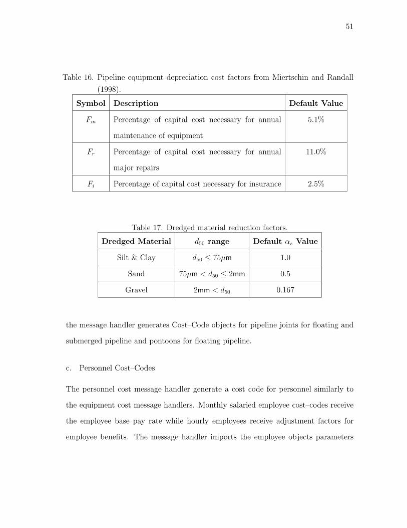
51

Table 16. Pipeline equipment depreciation cost factors from Miertschin and Randall

(1998).


Fm Percentage of capital cost necessary for annual

maintenance of equipment

5.1%

Fr Percentage of capital cost necessary for annual

major repairs

11.0%

Fi Percentage of capital cost necessary for insurance 2.5%

Table 17. Dredged material reduction factors.

Dredged Material d50 range Default αs Value

Silt & Clay d50 ≤ 75µm 1.0

Sand 75µm < d50 ≤ 2mm 0.5

Gravel 2mm < d50 0.167

the message handler generates Cost–Code objects for pipeline joints for floating and

submerged pipeline and pontoons for floating pipeline.

c. Personnel Cost–Codes

The personnel cost message handler generate a cost code for personnel similarly to

the equipment cost message handlers. Monthly salaried employee cost–codes receive

the employee base pay rate while hourly employees receive adjustment factors for

employee benefits. The message handler imports the employee objects parameters

52

Work-Area

+d50

Pipeline-Route

+Floating-Pipeline-Length = Lfl

+Submerged-Pipeline-Length = Lsu

+Shore-Pipeline-Length = Lsh

Cost-Code

+Dredge-Size = Dd

+Parent-Object = Pipeline-Route-Object, Pipeline-Equipment-Object+Depreciation-Cost = Cd

+Financing-Cost = Cf

+Quantity = Ns

Pipeline-Equipment

+Dredge-Size = Dd

+Capital-Cost = Cc

+Useful-Life = Tul

+Section-Length = ld+Standby-Rate = Sb

+Quantity = q

1

Fig. 20. Pipeline route cost–code object generation.

of pay–period (Pp), salary (Se), and minimum number (Nm). The message handler

then calculates the daily cost rate for monthly salaried employees from Miertschin

and Randall (1998) as:

Ce = Se12

365(3.9)

For hourly employees, the message handler determines the daily cost rate from


Ce = SeNhsNsd

(1 + βot +

Nh

365+Nv

365

)(1 + βss + βwc + βsu + βfu) (1 + βfr) (3.10)

Table 18 describes the cost parameters The message handler then generates a

Cost–Code object with the daily cost, minimum number, and the employee object

name as Figure 21 illustrates.

53

Table 18. Employee cost factors from Miertschin and Randall (1998).


Nhs Number of hours per shift 12.0

Nsd Number of shifts per day 1

βot Overtime factor 14.3%

Nh Holidays per year 13

Nv Vacation days per year 10

βss Social Security factor 2%

βwc Worker Compensation factor 45%

βsu State unemployment factor 3.5%

βfu Federal unemployment factor 1.0%

βfr Fringe benefits factor 1.0%

54

Cost-Code

+Dredge-Size = Dd

+Parent-Object = [Personnel-Object]+Daily-Cost = Ce

+Quantity = Nm

Personnel

+Dredge-Size = Dd

+Pay-Rate = Se

+Pay-Period = Pp

+MinNumber = Nm

1

Fig. 21. Personnel cost–code object generation.

2. Determine Task Duration

The DKBES uses message handlers to determine a task’s total duration from start to

finish. Each Task object contains a pointer to its associated Task–Method. Message

handlers associated with these task methods then calculate the duration based upon

the Task objects parameters.

a. Dredge Channel Task Determine Duration

The message handler that determines the duration of a Dredge–Channel Task uses

the results from the Pipeline Analytical Program and the properties of the Design–

Component objects. The Pipeline Analytical Program calculates the performance

metrics for the pump series in terms of in–situ production rate. The Design–Component

object associated with the task provides the total pipeline length and the work–area

object associated with the task provides the volume of in–situ material. Figure 22

55

Work-Area

+in-situ-Dredged-Material-Volume = Vmi

Design-Component

+Floating-Pipeline-Length = Ldf

+Submerged-Pipeline-Length = Ldu

+Shore-Pipeline-Length = Ldh

Dredge-Channel-Task

+Design-Component+Work-Area

Pump Series PerformanceMetrics Chart

M

Ld

1

Fig. 22. Objects used to calculate dredge channel duration from Miertschin and Ran-

dall (1998).

illustrates these object relations and Table 19 describes the variables. The message

handler calculates the duration of the task from Miertschin and Randall (1998) as:

Tdc =1

Tdp

VmiPmi

(3.11)

b. Mobilization and Demobilization

The DKBES determines the times required to mobilize and demobilize the pipeline

dredge project. The task methods contain message handlers that determine the time

required to transport, setup and store the pipeline and dredge. Tables 20 and 21

56

Table 19. Variables used to determine dredge–channel task duration from Miertschin

and Randall (1998).


Tdc Time to dredge channel section [days]

Tdp Average time dredge spends pumping [hrs/day] 16hrs/day

Vmi in–situ volume of dredged material [m3]

Pmi Production rate of in–situ dredged material

[m3/hr]

lists the formula the message handlers use to calculate each duration. Lt and Vt

represent the towing distance and speed, respectively. The DKBES uses default values

of 241km(150miles) and 161km/day(100miles/day) for these respective parameters.

The message handlers determine Ldf , Ldu, Ldh from the design–component object

parameters similarly to the message handler used to determine the duration for a

dredge–channel task.

3. Task–Costs

A dedicated message handler computes a task’s cost through its task method. This

message handler determines cost factors from the cost–code objects associated with

the equipment and personnel the task method requires. The message handler then

returns the total cost to assign to the task.

a. Mobilization and Demobilization

Message handlers calculate costs for the mobilization and demobilization tasks from

cost–code objects for equipment and personnel. The message handlers for each task–

57

Table 20. Pipeline mobilization durations from Miertschin and Randall (1998).

Task–Method Duration Formula

Prepare-dredge-for-transfer

Tmpd = 0.25Dd (3.12)

Prepare-pipeline-for-transfer

Tmpp = 0.0479 (Ldf + Ldu + Ldh)1/2 (3.13)

Transfer-pipeline

Tmtp =Lt

24Vt(3.14)

Transfer-dredge

Tmtd =Lt

24Vt(3.15)

Setup-pipeline

Tmsp = 0.7Tmpp(Ldf + 1.25Ldu + Ldh)

(Ldf + Ldu + Ldh)(3.16)

Setup-dredge

Tmsd = 1.0 (3.17)

58

Table 21. Pipeline demobilization durations from Miertschin and Randall (1998).

Task–Method Duration Formula

Prepare-dredge-for-transfer

Tdpd = 1.0 (3.18)

Prepare-pipeline-for-transfer

Tdpp = 0.6Tmsp (3.19)

Transfer-pipeline

Tdtp =Lt

24Vt(3.20)

Transfer-dredge

Tdtd =Lt

24Vt(3.21)

Store-pipeline

Tdsp = 1.0 (3.22)

Store-dredge

Tdsd = 1.0 (3.23)

59

method contain a list of equipment and personnel necessary for the task. Furthermore,

the message handler lists which equipment function as working and those that idle on

standby. The message handler then aggregates the daily cost of these cost–codes and

applies the task’s duration to compute a total task cost from Miertschin and Randall

(1998) as:

Cd = Ttask

(24

Nsb∑k=1

Csb(k) +Nwe∑k=1

Cwe(k) +

Npcc∑k=1

(Cp(k) + Csbs) + Cspt

)(3.24)

Cwe = Cd + Cf + Cfl (3.25)

Table 22 defines these variables. Table 23 describes the cost–code objects and

their function used to calculate cost of the prepare–pipeline-for–transfer–to–site and

prepare–pipeline-for–transfer–from–site tasks. Table 24 describes the cost–code ob-

jects and their function used to calculate cost of the prepare–dredge–for–transfer–to–

site and prepare–dredge–for–transfer–from–site tasks. Table 25 describes the cost–

code objects and their function used to calculate cost of the transfer–dredge, setup–

dredge, and store–dredge tasks. Table 26 describes the cost–code objects and their

function used to calculate cost of the transfer–pipeline, setup–pipeline and store–

pipeline tasks.

60

Table 22. Variables used to calculate task cost from Miertschin and Randall (1998).


Ttask Task duration [day]

Csb Hourly standby rate of equipment [$/hr]

Nsb Number of equipment on standby

Cwe Daily rate of working equipment [$/day]

Nwe Number of working equipment

Cp Daily working rate of personnel [$/day]

Csbs Daily subsistence rate for personnel [$/day] 25[$/day]

Npcc Number of personnel

Cspt Daily cost for supplies and tools [$/day] 100[$/day]

61

Table 23. Cost–code objects used to determine cost to prepare pipeline for transfer to

and from dredge sites from Miertschin and Randall (1998).

Object Class Function

Equipment

Pipeline Stand–by

Pipeline Joints Stand–by

Pipeline Pontoons Stand–by

Work tug Working

Crew tug Working

Fuel/water barge Working

Work barge Working

Derrick–Barge Working

Personnel

Shore–Crew Working

Table 24. Cost–code objects used to determine cost to prepare dredge for transfer to

and from dredge sites from Miertschin and Randall (1998).


Equipment

Dredge Stand–by

Booster–Pumps Stand–by

Personnel

Deck–Hand Working

62

Table 25. Cost–code objects used to determine cost to transfer the dredge from

Miertschin and Randall (1998).


Equipment

Dredge Stand–by

Booster–Pumps Stand–by

Crew tug Stand–by

Derrick Stand–by

Fuel/water barge Stand–by

Work barge Working

Personnel

Captain Working

Deckhand Working

Tug-Crew Working

63

Table 26. Cost–code objects used to determine cost to transfer, setup and store the

pipeline from Miertschin and Randall (1998).


Equipment

Pipeline Stand–by

Pipeline Joints Stand–by

Pipeline Pontoons Stand–by

Work barge Working

Personnel

Deckhand Working

64

b. Dredge Channel Task Determine Cost

The dredge channel task cost for a dredge channel task similarly to other task meth-

ods. The message handler calculates the cost of equipment and labor from cost–code

objects. However, the message handler determines the daily cost of dredge pump and

booster pumps based on the Pipeline Analytical Program performance metric calcu-

lation for pump power consumption. Table 27 describes the equipment and personnel

cost–code objects as well as their function in determining the dredge channel task’s

cost. The message handler determines the time to dredge the channel section from

the dredge–channel task determine duration message handler. The message handler

aggregates the daily costs of the equipment and personnel cost–code objects with the

exception of the dredge and pump objects. For these objects the message handler

uses the object parameters for depreciation and financing. For fuel and lube cost, the

message handler uses the performance metrics for pump power consumption from the

Pipeline Analytical Program. Figure 23 illustrates the cost–code objects parameters.

Table 28 describes the variables used to calculate the total cost of the dredge–channel.

The message handler calculates the total cost of the dredge–channel as:

Cday = Tdc

(Npcc∑k=1

Cp(k) +

Nnep∑k=1

(Cd(k) + Cf (k) + Cfl(k)) +

Nep∑k=1

(Cd(k) + Cf (k)) + (1 + fl)Ppump(k)fct100ff

)(3.26)

65

Table 27. Dredge channel task cost–codes from

Miertschin and Randall (1998).


Equipment

Pipeline-Dredge Working

Work-Tug Working

Crew-Survey-Tug Working

Derrick Working

Fuel-Water-Barge Working

Work-Barge Working

Pipeline Working

Joints Working

Pontoons Working

Booster-Pumps Working

Personnel

Captain Working

Officer Working

Chief-Engineer Working

Office-Help Working

Leverman Working

Dredge-Mate Working

Tug-Crew Working

Equipment-Operator Working


66

Table 27. Continued.


Welder Working

Deckhand Working

Electrician Working

Dump-Foreman Working

Shore-Crew Working

Oiler Working

Table 28. Variables used to calculate dredge channel task cost.

Symbol Description

Nnep Number of equipment not pumping related

Ppump Pipeline Analytical Program calculated pumping

power [kW]

Nep Number of pumping related equipment

67

Equipment-Cost-Code

+Depreciation-Cost = Cdep

+Financing-Cost = Cfin

+Fuel-Lube-Cost = Cfuel

Personnel-Cost-Codes

+Daily-Working-Rate = Cp

Non-Dredge and Non-PumpCost-Code Objects

Equipment-Cost-Code

+Depreciation-Cost = Cdep

+Financing-Cost = Cfin

Dredge and PumpCost-Code Objects

Pump Series PerformanceMetrics Chart

P(bhp)

Ld

1

Fig. 23. Objects used to calculate dredge channel cost.

68

Fig. 24. Gantt chart output of the pipeline dredge project.

c. Ancillary Message Handlers

Message handlers format the output for the graphical scheduling output of the result-

ing pipeline dredge project to a Gantt chart program. The message handler calls the

mobilization, dredging and de–mobilization activities and iterates through their sub–

activities and tasks exporting their start–date, duration, end–date and precedence

parameters to the charting program. Figure 24 illustrates the resulting Gantt chart

output.

C. Process Modules

The DKBES uses four process modules to formulate a pipeline dredge project. These

modules use the existing knowledge–base of equipment, personnel and task–method

objects as well as project specific objects for design–components, work–areas and

dredged–material.

1. Design–Initialization

The Design–Initialization Module generates the dredge project activities based on

the pipeline dredge, work area and pipeline route specified in the design–component

69

Fig. 25. Initial design of pipeline dredge project.

object. This module uses a rules–base to construct the activities, sub–activities and

tasks necessary to execute the dredge project from start to finish. These rules assign

tasks to activities and sub–activities and define the precedence relationship between

mobilization, demobilization and channel dredging. While the rules construct the

order of the pipeline dredge project, they leave out definitive time schedules and

start or end times. Figure 25 illustrates the resulting initial design.

70

a. Build–Mobilization–Demobilization

The Build–Mobilization module rules will generate a mobilization activity for a Design–

Component object. Mobilization requires several sub–activities and tasks. Table 29

describes the mobilization activities and their sub–activities and tasks.

Table 29. Precedence factors for mobilization activities and tasks.

Sub–Activities and Tasks Preceded-By

Prep-For-Transfer-To-Site-Activity None

Prep-Dredge-Task None

Prep-Pipeline-Task None

Transfer-To-Site-Activity Prep-For-Transfer-To-Site-Activity

Transfer-Dredge-To-Site None

Transfer-Pipeline-To-Site None

Setup-Dredge-Pipeline-Activity Transfer-To-Site-Activity

Setup-Dredge-Task None

Setup-Pipeline-Task None

b. Dredging–Activity

The DKBES generates the dredging activity and tasks according to the work areas

specified in the design–component object. The dredging activity rules-base generates

a Dredge–Channel task for each work area in the design component. A Dredge–

Channel activity contains each Dredge–Channel tasks for the Design–Component

object. Each Dredge–Channel task will contain a Dredge–Channel task method. The

71

rules will order the Dredge–Channel tasks by setting the preceded–by attribute to

the Dredge–Channel task of the work area before it in sequence.

c. Build–Demobilization

The Build–Demobilization rules will generate a demobilization activity for a Design–

Component object. Table 30 describes the demobilization activities and their sub–

activities and tasks.

Table 30. Precedence factors for demobilization activities and tasks.

Sub–Activities and Tasks Preceded-By

Prep-For-Transfer-From-Site-Activity

Prep-Dredge-Task

Prep-Pipeline-Task

Transfer-From-Site-Activity Prep-For-Transfer-From-Site-

Activity

Transfer-Dredge-From-Site

Transfer-Pipeline-From-Site

Prepare-For-Storage-Activity Transfer-From-Site-Activity

Store-Dredge-Task

Store-Pipeline-Task

2. Initial–Scheduling

The Initial–Scheduling module contains the rules–base to determine the duration of

each task within the initial design. The rules–base applies the message handlers

that determine the duration of each task according to its task–method. This module

72

Fig. 26. Initial scheduling of pipeline dredge project.

establishes the time necessary to complete each task within the dredge design will

leaving out any calculation to determine the start or end date of the tasks or activities.

Figure 26 illustrates the resulting initial scheduling.

3. Detailed–Scheduling

The Detailed–Scheduling module determines the rigid schedule of the dredge project

by establishing actual start dates and end dates for each activity and their sub–

activities and tasks. The first rule determines tasks and activity start dates by tasks

and activities that precede them. A task or activity cannot start before any task or

activity that precedes it completes. The second rule evaluates sub–activities and tasks

within an activity. Sub–activities and tasks cannot start before their main activity

can start. The rules will set the start and end dates of the tasks and activities

according to these criteria. Figure 27 illustrates the resulting detailed schedule.

73

Fig. 27. Detailed scheduling of pipeline dredge project.

4. Cost–Distribution

The Cost–Distribution module determines the aggregate cost of activities, sub–activities

and tasks. The rules–base for this module first constructs cost–code objects for all

the equipment and personnel objects within the knowledge–base. A rule determines

the aggregate cost of each task by applying the message handlers that determine the

cost associated with each task. Finally, rules will determine the aggregate cost of

activities and sub–activities by the sum of their activity costs.

74

D. DKBES Architecture Summary

The DKBES object–oriented architecture provides the knowledge–base expert–system

the versatility to solve a pipeline dredge projects based on common attributes of

the pipeline dredge components. The classes structure the components into objects.

Message handlers calculate the object parameters based on class. Rules define the

work flow of the pipeline dredge project based on the objects and message handlers

that process their attribute values.

75

CHAPTER IV

GOETZ FIELD DATA COLLECTION

The U.S. Army Corps of Engineers pipeline dredge Goetz, a 508mm(20in) cutterhead

pipeline dredge with a single onboard dredge pump, collected dredge production data

on June 22, 2009 from onboard dredge instrumentation while dredging on the Upper

Mississippi River near St. Paul, Minnesota. The dredge production data can provide

insight and understanding as to how well the theoretical and empirical equations for

pipeline hydraulics and slurry transport compares to actual dredge production. Anal-

ysis of the dredge instrumentation data can verify how well the Pipeline Analytical

Program can predict production rate on a cutterhead pipeline dredge based on pump

and pipeline parameters.

A. Goetz Description

Table 31 describes the Goetz pipeline dredge parameters involved in the dredging

project on the Upper Mississippi River. Figure 28 illustrates the Goetz dimensionless

pump performance curves. Figure 29 illustrates the dredge pipeline parameters and

the dredge pump instrumentation. Table 32 describes the onboard instrumentation

data parameters the Goetz collects. TDH measurements require further calculation

from the instrumentation data where:

TDHs =Pd − PsSmdγw

+16π2

2g

(1

D4d

− 1

D4s

)Q2 (4.1)

76

Table 31. Dredge Goetz Pipeline Dredge pump and pipeline system parameters.

Symbol Description Value

Dd Discharge pipe diameter (m) 0.508m(20in)

Ds Suction pipe diameter (m) 0.559m(22in)

Di Pump impeller diameter (m) 1.370m(54in)

Ls Suction length (m) 11.0m(36ft)

Zd Digging depth (m) 3.7m(12ft)

Zb Discharge elevation (m) 24.1m(79ft)

Zp pump elevation (m) 0.5m(1.64ft)

Ld Pipeline discharge length (m) 627.7m(2,059ft)


εs Pipe relative roughness (mm) 0.508mm(0.02in)



µw Water viscosity (P·s) 10−3P·s

g Gravitational acceleration(m/s2) 9.81m/s2

ρs Solid particle density(kg/m3) 2,650kg/m3

d50 Median sediment grain diameter(mm) 0.1mm

xf in–situ fine material fraction 0.1

Smd Specific gravity of pipeline slurry

Smi Specific gravity of in–situ material



Ha Atmospheric Pressure Head (mH2O) 10.4 (mH2O)

Hv Vapor Pressure Head (mH2O) 0.18(mH2O)

77

0.2

0.4

0.6

0.8

1

1.2

1.4

0 0.2 0.4 0.6 0.8 1

Hdi

m ×

101 ,

NP

SHR

dim

×10

2

Qdim ×102

Dimensionless Pump Curve Dredge Goetz

Pump HDP 550-1370-280-3 Ds=560mm(22in), Dd=510mm(20in), Di=1370mm(54in)

0 0.2 0.4 0.6 0.8 10

10

20

30

40

50

60

70

Eff

%

Hdim

NPSHRdim

Eff

Fig. 28. Dredge Goetz dimensionless pump curve.

Fig. 29. Dredge Goetz pump and pipeline system configuration.

78

Table 32. Pipeline dredge Goetz Silent Inspector parameters.

Pipeline Dredge Parameter Pipeline Dredge Instrument

Zd Inclinometer

RPM Pump RPM meter

Ps Pump suction pressure gauge

Pd Pump discharge pressure gauge

Vd Pump discharge velocity meter

Smd Nuclear density meter

79

B. Dimensionless Pump Data Analysis

Dimensionless pump parameters indicate how well the dredge instrumentation data

coincide to the dredge pump performance curve. Figure 30 illustrates the comparison

of the actual dimensionless pump data of dimensionless flow rate, Qdim, and dimen-

sionless head, TDHdim, from the dredge instrumentation data to the pump curve

dimensionless data where:

Qdim =Q

ωD3i

(4.2)

TDHdim =TDHsg

ω2D2i

(4.3)

The actual dimensionless head consistently exceeded the theoretical dimension-

less curve. Figure 31 illustrates the residuals between the actual dimensionless head

and the theoretical dimensionless head according to the pump curve data where:

RESTDHdim= TDHdim(actual)− TDHdim(theoretical) (4.4)

Specific gravity presents the only noticeable pattern of residuals where the resid-

uals decrease steadily when specific gravity increases.

80

0.125

0.13

0.135

0.14

0.145

0.15

0.155

0.16

0 0.002 0.004 0.006 0.008 0.01

Hdi

m

Qdim

Dimensionless Dredge Instrumentation Data Dredge Goetz

Pump HDP 550-1370-280-3 Ds=560mm(22in), Dd=510mm(20in), Di=1370mm(54in)

Fig. 30. Dredge Goetz dimensionless pump curve as well as Silent Inspector data.

81

-2

0

2

4

6

8

10

10 20 30 40 50 60

Res

id [

m s

lurr

y]

Predicted TDH [m slurry]

-2

0

2

4

6

8

10

20 30 40 50 60 70

Actual TDH [m]

-2

0

2

4

6

8

10

1 1.1 1.2 1.3 1.4

Res

id [m

slu

rry]

Smd

-2

0

2

4

6

8

10

200 300 400RPM

-2

0

2

4

6

8

10

2 3 4 5

Res

id [m

slu

rry]

Vd m/s

-2

0

2

4

6

8

10

0 1 2 3 4Zd [m]

Residual Analysis of TDHCompared to Pump Curve

Fig. 31. Residual analysis of Dredge Goetz dimensionless pump curve data compared

to Silent Inspector data.

82

0

20

40

60

80

100

120

140

160

0 0.2 0.4 0.6 0.8 1 1.2 1.4

TD

H s

lurr

y [m

]

Q [m3/s]

Goetz Pump and Pipeline System Data Ld=627.74m (2,059ft), Dd=508mm(20.0in), Ds=559mm(22.0in), d50=0.10mm

Smd=1.0

Smd=1.1

Smd=1.2Smd=1.3

Smd=1.4

Smd=1.5

EquivalentFlow Rateby TDHsQeq= 0.96m3/s

EquivalentFlow Rate

by imQeq= 0.86m3/s

Qsm

400RPM425RPM450RPM

Fig. 32. Dredge Goetz pipeline pump and pipeline system curves as well as Silent

Inspector data.

C. Pipeline System Data Comparison

The theoretical system head curves based on the Wilson et al. (1997) equations showed

some interesting comparison to the actual dredge pump data. Figure 32 shows the

system head curves for a range of specific gravities and the actual Silent Inspector

system data. The theoretical pipeline system curves fall right down the center of the

distribution of Silent Inspector data suggesting that the Wilson et al. (1997) equations

provide a suitable average for the actual data.

Pipeline system curves intersect the pump performance curves corresponding to

450 RPM at the pipeline system flow rate of equivalent fluid, Qeq, where the pipeline

system curves act independent of specific gravity. The Wilson et al. (1997) equations

83

estimate Qeq as the flow rate where the friction gradient for a slurry equals the friction

gradient for the carrier fluid as:

imdSm

= iwd (4.5)

imd = 0.22 (Sm − 1)

(V50

Veq

)1.7

(4.6)

iwd =fwdV

2eq

2gDd

(4.7)

iwdSm = iwd + 0.22 (Sm − 1)

(V50

Veq

)1.7

(4.8)

iwd (Sm − 1) = 0.22 (Sm − 1)

(V50

Veq

)1.7

(4.9)

iwd = 0.22

(V50

Veq

)1.7

(4.10)

V 1.7eq = V 1.7

50

(0.22

iw

)(4.11)

V 1.7eq = 0.22V 1.7

50

(2gDd

fwdV 2eq

)(4.12)

V 3.7eq = 0.22V 1.7

50

(2gDd

fwd

)(4.13)

Veq = V 0.46050

(0.44gDd

fwd

)0.270

(4.14)

Qeq = VeqπD2

d

4(4.15)

84

This equation, however, does not account for static lift due to digging depth or

friction losses in the suction side of the pump. A more thorough calculation accounts

for these factors by determining:

TDHw = TDHs (4.16)

��Zb +�

��

�Σkd

V 2d

2g+

��

��

ΣksV 2s

2g+ �

�V 2d + iwdLd + iwsLs = Zd

Sm − 1

Sm+ ��Zb+

��

��

ΣkdV 2d

2g+

��

��

ΣksV 2s

2g+ �

�V 2d +

imdLdSm

+imsLsSm

(4.17)

Canceling common terms to both sides and expanding iw and im yields:

fwdV2d

2gDd

Ld +fwsV

2s

2gDs

Ls = ZdSm − 1

Sm+

fwdV2d

2gDdSmLd

+fwsV

2s

2gDsSmLs + 0.22

Sm − 1

Sm

V 1.750s

V 1.7s

Ls + 0.22Sm − 1

Sm

V 1.750d

V 1.7d

Ld (4.18)

Vd =4Qeq

πD2d

(4.19)

Vs =4Qeq

πD2s

(4.20)

16

2gπ2

(fwdLdD5d

+fwsLsD5s

)Q2eq = Zd+0.22

(π4

)1.7 1

Q1.7eq

((V50sD

2s

)1.7Ls +

(V50dD

2d

)1.7Ld

)(4.21)

Since this equation cannot solve for the Qeq explicitly, a computer program must

solve for the polynomial root of the equation. At this flow rate, the actual TDH

and flow rate of a pipeline system would not depend heavily on the density of the

mixture transported in the pipe. The pump and pipeline analytical program could

determine the intersection of the pump and pipeline system without significant error

85

caused by inaccurate density assumptions. Figure 32 illustrates the Qeq calculated

from both Wilson et al. (1997) method and by equating TDHs for slurry and water.

Both methods come reasonably close to the actual intersections of the pipeline system

curves. The TDH method provides a more accurate result with some error due to

fw and V50 ultimately varying with Smd. Figure 33 illustrates the residual analysis of

the actual system TDH compared to the theoretical pipeline system curves where:

RESTDHs = TDHs(actual)− TDHs(theoretical) (4.22)

Figure 33 shows high correlation with both specific gravity suggesting that the Wilson

et al. (1997) equations provide a more precise calculation at higher density slurries

rather than water.

D. Maximum Production Data Comparison

The Pipeline Analytical Program compared the Goetz production data to the the-

oretical maximum production based on vacuum limitation of the pump. Analysis

calculated NPSHA for the pump based on dredge instrumentation data as:

NPSHA =Ha −Hv

Smd+

PsρwgSmd

+V 2s

2g(4.23)

Vs =D2d

D2s

Vd (4.24)

For a range of flow rates, the Pipeline Analysis Program calculates Smd where

NPSHA equal NPSHR from the pump curve data in Figure 28. Figure 34 illustrates

the curve of this maximum production relationship. The program further calculated

the time–averaged delivered specific gravity, Smd, at 1.067 as Figure 35 illustrates.

The Pipeline Analytical Program calculated the optimum Smd as 1.60. All dredge

86

Fig. 33. Residual analysis of Dredge Goetz pipeline system curves compared to Silent

Inspector data.

87

0

200

400

600

800

1000

1200

1400

0 0.5 1 1.5 2

Dry

Sol

ids

Pro

duct

ion

Rat

e [m

3 /hr]

Flow Rate, Q [m3/s]

Maximum Production Rate Due to Pump Vacuum LimitationDredge Goetz, Pump HDP-550-1370-280-4


Zd

500RPM

Smd=1.06

Smd=1.10

Smd=1.20

Smd=1.30

S md=1.40

S md=1.60

S md=1

.80

Max Smd=1.79

Opt Smd=1.57

Fig. 34. Dredge Goetz maximum production curve.

production data fell well below this mark with the maximum Smd at 1.40. This

result suggests the Goetz can capably dredge denser mixtures than the cutterhead

can actually pursue.

88

12:30 12:45 13:00 13:15 13:30 13:451

1.05

1.1

1.15

1.2

1.25

1.3

1.35

1.4

Time [HH:MM]

Sm

d

Silent Inspector Data for Specific GravityDredge Goetz June 22, 2009Pump HDP 550−1370−280−4

Ds=560mm(22in), Dd=508mm(20in), D

i=1370mm (54in)

Smd

Mean Smd

Fig. 35. Dredge Goetz time–averaged Smd.

89

E. Dredge Production Analysis

The Pipeline Analytical Program analyzed production of the Goetz operation in the

Upper Mississippi River on June 22, 2009 based on the dredge pump and pipeline sys-

tem parameters. The Pipeline Analytical Program used pump data from the dredge

pump performance curves and the pipeline system data to compute the operating

point based on the interaction between the two. The Pipeline Analytical Program

then computed the resulting production rate of the dredged material to compare with

the actual results of the Goetz dredge instrumentation data.

The Pipeline Analytical Program calculated the operating parameters of the

dredge Goetz operating under the pipeline system parameters in Table 31 and the

pump performance curves in Figure 32. The Pipeline Analytical Program uses maxi-

mum operating parameters for pump shaft speed and pump shaft power as 425RPM

and 1,192kW(1,600bhp), respectively. Figure 36 illustrates the pump and generated

pipeline system curves. Table 33 shows the Pipeline Analytical Program calculated

performance metrics. The Pipeline Analytical Program compared these performance

metrics to the Goetz Silent Inspector data by calculating the actual delivered volume

of dry material over a time–span, tj, as:

Volumeactual(tj) =

j∑i=2

1

2

(Mi + Mi−1

)(ti − ti−1) (4.25)

This method uses the trapezoidal rule to numerically integrate production rate.

The Pipeline Analytical Program calculates the theoretical volume of dry material

from the theoretical production rate as:

V olumetheoretical(tj) = Mtheoretical (tj − t1) (4.26)

90

40

50

60

70

80

90

0 50 100 150 200

TD

H [m

slu

rry]

Dredge Pump and System Performance Curves Pump 1 HDP-550-1370-280-4

Production Rate Dry Material [m3/hr]

0 0.2 0.4 0.6 0.8 1 1.2 1.4 1.6

40

50

60

70

80

90

TDH [m slurry]

Flow Rate [m3/s]

Ld=6

27m

400RPM

425RPM

450RPM

475RPM

500RPM

525RPM

550RPM40%45%50% 55% 60% 65%

68%71%

74%77%

500kW 700kW

900kW

1,100kW

1,300kW

1,500kW

Q=0.94m3/sH=55m

Fig. 36. Pipeline Analytical Program results for Dredge Goetz dredging project.

91

Table 33. Dredge Goetz Pipeline Analytical Program performance parameter results.

Performance Parameter Value

Smi 1.62

cvi 0.38

Fb 1.91

ηbh 0.35

ηd 0.75

cvd 0.037

Smd 1.057

Q 0.94m3/s(33.24ft3/s)

TDHs 55m(181.8ft)

M 139.1 m3/hr(181.1yd3/hr)

Figure 37 illustrates the timeline of cumulative volume of dry material based on

actual Silent Inspector production measurements and the theoretical pipeline equa-

tions as well the percent difference between the actual and theoretical volume as:

V olume%difference =V olumeactual(tj)− V olumetheoretical(tj)

V olumeactual(tj)× 100 (4.27)

The Pipeline Analytical Program calculated the final actual and theoretical dry

material production of 191.6m3 and 205.2m3, respectively, making a 6.62% percent

difference.

92

Fig. 37. Production comparison between Pipeline Analytical Program results and

Silent Inspector data results.

93

F. Results and Discussion

The actual Silent Inspector pipeline dredge production data compared well with the

Wilson et al. (1997) equations for the TDH by illustration of the pipeline system

curves in Figure 32. Residual analysis between the actual TDH values and TDH

obtained by Wilson et al. (1997) equations show the strongest dependence on velocity.

Likewise, residual analysis between actual TDHdim and TDHdim obtained from the

pump performance curve as shown in Figure 31 showed velocity as the strongest

influencing factor and correlation between actual and theoretical values.

The dimensionless head curve in Figure 30 shows that the dredge instrumentation

data exceed the manufacturers pump performance curve. This suggests suggests some

error in the dredge instrumentation.The Pipeline Analytical Program calculated Q

for the dredge pump and pipeline system relatively close to the equivalent fluid flow

rate, Qeq. This measurement suggests the Goetz operates at a flow rate that stays

constant despite change in the Smd to simplify dredge operation.

The pipeline analytical program calculated a dry material production rate of

139.1m3/hr that translates to a final production of final dredged material produc-

tion of 191.6m3 compared with 205.2m3 of actual production with a net difference of

6.62%. The dredge instrumentation measured an average Smd of 1.067. The Pipeline

Analytical Program calculated Smd of 1.057 based on empirical formula for the Fb and

Smi based on the fines fraction, xf . Furthermore, the Pipeline Analytical Program

needed to estimate a value for the xf in lieu of sediment laboratory analysis. Although

these values represent reasonable estimates to determine the delivered slurry concen-

tration and ultimate production, actual sediment analysis would help to show that

the Pipeline Analytical Program does produce verifiable results for pipeline dredge

production.

94

CHAPTER V

PIPELINE DREDGE PROJECTS

Daily dredge reports from two U.S. Army Corps of Engineers districts provide a

comparison between the Pipeline Analytical Program and the actual pipeline dredge

production throughout the entire span of a dredge project. Daily dredge reports

contain the daily pipeline dredge progress throughout the project lifecycle. Table 34

describes these daily data parameters. The actual names of the dredges and their

project numbers have been obfuscated in order to protect potentially proprietary

data. These data will lend considerable evidence as to how accurately the Pipeline

Analytical Program can calculate the daily production of a pipeline dredge project

protracted over many months.

Table 34. Daily dredge report data parameters

Data Parameter Description

Date Date of dredging activity

V ol Daily volume of dredged material [m3]

Zi Initial depth of channel [m]

Zd Design dredging depth [m]

Ld Pipeline Length [m]

ADV Pipeline dredge advance [m]

Tp Total time dredging [hours]

Pump Series Pumps used in the pump series

Given these pump and pipeline operating parameters, the Pipeline Analytical

Program determines the theoretical daily dredge production. Analysis compares the

95

% difference between actual production data and theoretical production as:

M%difference =Mactual(tj)− Mtheoretical(tj)

Mactual(tj)× 100 (5.1)

Analysis further compares % difference between actual cumulative volume and

theoretical cumulative volume as:

V olume%difference =V olumeactual(tj)− V olumetheoretical(tj)

V olumeactual(tj)× 100 (5.2)

Residual analysis compares the difference between actual and theoretical produc-

tion rate as:

RESproduction = M(actual) − M(theoretical) (5.3)

A. Savannah District Project Data

The USACE Savannah District dredges 4.57 million m3(6 million yd3) per year

from the Savannah River to maintain 15.5m (51ft) navigable depth. Three dredging

projects from 2000 and 2003 provide daily dredge report data to compare actual

dredge project data to the Pipeline Analytical Program. All three projects used

Dredge A, an 457mm(18in) cutterhead pipeline dredge. Table 35 describes A’s dredge

parameters.

1. Dredge A Project 1

Table 36 describes the pump system data for Project 1 on the Savannah River us-

ing Dredge A. Figures 38–40 contain the Pipeline Analytical Program results for the

pump and pipeline interaction. Figure 41 illustrates the composite pump series and

pipeline performance curves. Figure 42 illustrates the performance metrics of produc-

tion and power consumption with pipeline length. Figure 43 illustrates the maximum

96

Table 35. Dredge A parameters

Dredge Parameter Value

Dd 457mm(18in)

Ds 457mm(18in)

Ls 12.2m(40ft)

LL 26.3m(83ft)

Dc 2.13m(7ft)

Zlp -6.1m(-20ft)

production capable of the first pump limited by cavitation. as the performance met-

rics of theoretical production rate with respect to pipeline length. Figure 44 shows

the timeline comparison between actual dredge production and theoretical dredge

production. Figure 45 contains the residual plot between the actual and theoretical

production rates compared with the dredging parameters for data comparison.

Table 36. Dredge A pump parameters for Project 1.

Name Di Power Max RPM

Ladder MPMW-18x18x34 863mm(34in) 372kW(500bhp) 500

Hull LSA-18x18-44-4 1,117mm(44in) 875kW(1,175bhp) 600


97

Fig. 38. Pump 1 curves for Dredge A on Project 1.


98


Fig. 41. Pump series composite curve for Dredge A on Project 1.

99

Fig. 42. Pump series performance metrics for Dredge A on Project 1.

Fig. 43. Ladder pump maximum production curve for Dredge A on Project 1.

100

2000−11−19 2000−11−26 2000−12−03 2000−12−10 2000−12−17 2000−12−24 2000−12−31 2001−01−070

1000

2000

Pro

duct

ion

Rat

ein

−si

tu M

ater

ial [

m3 /h

r]Dredge A Dredging Savannah River

Contract 1 Nov.21,2000−Jan.03,2001Pump Series: MPMW−18x18x34, LSA−18x18−44−4, LSA−18x18−44−4

Ds=457mm(18in), D

d=457mm(18in), Z

d=16m(51ft)

Percent Difference Actual Theoretical

−50

0

50

100

Per

cent

Diff

eren

ce

2000−11−19 2000−11−26 2000−12−03 2000−12−10 2000−12−17 2000−12−24 2000−12−31 2001−01−070

5

10x 10

5

Cum

ulat

ive

Vol

ume

in−

situ

Mat

eria

l [m

3 ]

2000−11−19 2000−11−26 2000−12−03 2000−12−10 2000−12−17 2000−12−24 2000−12−31 2001−01−0720

30

40

50

Per

cent

Diff

eren

ce

2000−11−19 2000−11−26 2000−12−03 2000−12−10 2000−12−17 2000−12−24 2000−12−31 2001−01−070

10

20

30

40

Tim

e−P

umpi

ng [h

r]

2000−11−19 2000−11−26 2000−12−03 2000−12−10 2000−12−17 2000−12−24 2000−12−31 2001−01−072000

2500

3000

3500

4000

L d [m]

2000−11−19 2000−11−26 2000−12−03 2000−12−10 2000−12−17 2000−12−24 2000−12−31 2001−01−070

1

2

3

4

Cut

Fac

e,H

b [m]

2000−11−19 2000−11−26 2000−12−03 2000−12−10 2000−12−17 2000−12−24 2000−12−31 2001−01−0714

14.5

15

15.5

16

Dre

dge

Dep

th,

Zd [m

]

2000−11−19 2000−11−26 2000−12−03 2000−12−10 2000−12−17 2000−12−24 2000−12−31 2001−01−070

100

200

300

400

Dre

dge

Adv

ance

[m]

Fig. 44. Comparison between actual dredge production and theoretical dredge produc-

tion for Dredge A on Project 1.

101

200 400 600 800−200

0

200

400

600

800

1000

Theoretical Production [m3/hr]

Res

idua

ls [m

3 /hr]

0 1000 2000−200

0

200

400

600

800

1000

Actual Production [m3/hr]

Res

idua

ls [m

3 /hr]

Residual Analysis of Actual and Theoretical Production DataDredge A Dredging Savannah River

Contract 1 Nov.21,2000−Jan.03,2001Pump Series: MPMW−18x18x34, LSA−18x18−44−4, LSA−18x18−44−4

Ds=457mm(18in), D

d=457mm(18in), Z

d=16m(51ft)

0 10 20 30−200

0

200

400

600

800

1000

Time−Pumping [hr]

Res

idua

ls [m

3 /hr]

2000 2500 3000 3500−200

0

200

400

600

800

1000

Ld [m]

Res

idua

ls [m

3 /hr]

0 1 2 3−200

0

200

400

600

800

1000

Hb [m]

Res

idua

ls [m

3 /hr]

14 15 16−200

0

200

400

600

800

1000

Zd [m]

Res

idua

ls [m

3 /hr]

0 100 200 300−200

0

200

400

600

800

1000

Advance [m]

Res

idua

ls [m

3 /hr]

Fig. 45. Residual analysis between actual dredge production and theoretical dredge

production for Dredge A on Project 1.

102


In 2003, Dredge A dredged Savannah River using two separate dredged material place-

ment sites. The first placement site required at most 3,140m(10,300ft) of pipeline.

The second placement site required 12,957m(42,500ft). The pipeline analytical pro-

gram analyzes the 2003 project as a short–distance and long–distance application.

Tables 37 and 38 describe the pump configuration for these two applications.

Figures 46–52 illustrate the pump and pipeline performance curves, the series

composite performance curve, the system performance metrics and the maximum

ladder pump production rate for the short–distance pipeline application. Figure 53

shows the timeline comparison between actual dredge production and theoretical

dredge production. Figure 54 contains the residual plot between the actual and theo-

retical production rates compared with the dredging parameters for data comparison.







103

Fig. 46. Pump 1 curves for Dredge A in Savannah River on Project 2.


104



105

Fig. 50. Pump series composite curve for Dredge A in Savannah River on Project 2.

Fig. 51. Pump series performance metrics for Dredge A in Savannah River on Project

2.

106

Fig. 52. Ladder pump maximum production curve for Dredge A in Savannah River on

Project 2.

107

2003−07−01 2003−08−01 2003−09−01 2003−10−01 2003−11−01 2003−07−01 2003−08−01 2003−09−01 2003−10−010

1000

2000

Pro

duct

ion

Rat

ein

−si

tu M

ater

ial [

m3 /h

r]Dredge A Dredging Savannah RiverContract 2 Jul.16,2003−Oct.12,2003

Pump Series: MPMW−18x18x34, LSA−18x18−44−4, LSA−18x18−44−4, LSA−18x18−44−4D

s=457mm(18in), D

d=457mm(18in), Z

d=16m(51ft)


−1000

−500

0

500

Per

cent

Diff

eren

ce

2003−07−01 2003−08−01 2003−09−01 2003−10−01 2003−11−01 2003−07−01 2003−08−01 2003−09−01 2003−10−010

0.5

1

1.5

2x 10

6

Cum

ulat

ive

Vol

ume

in−

situ

Mat

eria

l [m

3 ]

2003−07−01 2003−08−01 2003−09−01 2003−10−01 2003−11−01 2003−07−01 2003−08−01 2003−09−01 2003−10−010

10

20

30

Per

cent

Diff

eren

ce

2003−07−01 2003−08−01 2003−09−01 2003−10−01 2003−11−01 2003−07−01 2003−08−01 2003−09−01 2003−10−010

10

20

30

40

Tim

e−P

umpi

ng [h

r]

2003−07−01 2003−08−01 2003−09−01 2003−10−01 2003−11−01 2003−07−01 2003−08−01 2003−09−01 2003−10−010

1000

2000

3000

4000

L d [m]

2003−07−01 2003−08−01 2003−09−01 2003−10−01 2003−11−01 2003−07−01 2003−08−01 2003−09−01 2003−10−010

1

2

3

4

Cut

Fac

e,H

b [m]

2003−07−01 2003−08−01 2003−09−01 2003−10−01 2003−11−01 2003−07−01 2003−08−01 2003−09−01 2003−10−0111

11.5

12

12.5

13

Dre

dge

Dep

th,

Zd [m

]

2003−07−01 2003−08−01 2003−09−01 2003−10−01 2003−11−01 2003−07−01 2003−08−01 2003−09−01 2003−10−010

100

200

300

400

Dre

dge

Adv

ance

[m]


tion for Dredge A in Savannah River on Project 2.

108

0 500 1000 1500−1000

−500

0

500

1000

1500


Res

idua

ls [m

3 /hr]

0 1000 2000−1000

−500

0

500

1000

1500


Res

idua

ls [m

3 /hr]

Residual Analysis of Actual and Theoretical Production DataDredge A Dredging Savannah RiverContract 2 Jul.16,2003−Oct.12,2003

Pump Series: MPMW−18x18x34, LSA−18x18−44−4, LSA−18x18−44−4, LSA−18x18−44−4D

s=457mm(18in), D

d=457mm(18in), Z

d=16m(51ft)

0 10 20 30−1000

−500

0

500

1000

1500

Time−Pumping [hr]

Res

idua

ls [m

3 /hr]

0 2000 4000−1000

−500

0

500

1000

1500

Ld [m]

Res

idua

ls [m

3 /hr]

0 2 4−1000

−500

0

500

1000

1500

Hb [m]

Res

idua

ls [m

3 /hr]

11.5 12 12.5 13−1000

−500

0

500

1000

1500

Zd [m]

Res

idua

ls [m

3 /hr]

0 200 400−1000

−500

0

500

1000

1500

Advance [m]

Res

idua

ls [m

3 /hr]


production for Dredge A in Savannah River on Project 2.

109


Figures 55–62 illustrate the pump and pipeline performance curves, the series com-

posite performance curve, the system performance metrics and the maximum ladder

pump production rate for the long–distance pipeline application. Figure 63 shows










Booster LSA-18x18-44-4 1,117mm(44in) 2,235kW(3,000bhp) 600

110



111



112


Fig. 60. Pump series composite curve for Dredge A in Savannah River on Project 3.

113

Fig. 61. Pump series performance metrics for Dredge A in Savannah River on Project

3.

Fig. 62. Ladder pump maximum production curve for Dredge A in Savannah River on

Project 3.

114

2003−10−01 2003−11−01 2003−12−01 2004−01−01 2003−10−01 2003−11−01 2003−12−01 2004−01−01 2003−10−01 2003−11−010

1000

2000

Pro

duct

ion

Rat

ein

−si

tu M

ater

ial [

m3 /h

r]Dredge A Dredging Savannah River

Contract 3 Oct.28,2003−Dec.17,2003Pump Series: MPMW−18x18x34, LSA−18x18−44−4, LSA−18x18−44−4, LSA−18x18−44−4, LSA−18x18−44−4

Ds=457mm(18in), D

d=457mm(18in), Z

d=16m(51ft)


−200

−100

0

100

Per

cent

Diff

eren

ce

2003−10−01 2003−11−01 2003−12−01 2004−01−01 2003−10−01 2003−11−01 2003−12−01 2004−01−01 2003−10−01 2003−11−010

5

10x 10

5

Cum

ulat

ive

Vol

ume

in−

situ

Mat

eria

l [m

3 ]

2003−10−01 2003−11−01 2003−12−01 2004−01−01 2003−10−01 2003−11−01 2003−12−01 2004−01−01 2003−10−01 2003−11−01−50

0

50

Per

cent

Diff

eren

ce

2003−10−01 2003−11−01 2003−12−01 2004−01−01 2003−10−01 2003−11−01 2003−12−01 2004−01−01 2003−10−01 2003−11−010

10

20

30

40

Tim

e−P

umpi

ng [h

r]

2003−10−01 2003−11−01 2003−12−01 2004−01−01 2003−10−01 2003−11−01 2003−12−01 2004−01−01 2003−10−01 2003−11−011.2

1.22

1.24

1.26

1.28

1.3x 10

4

L d [m]

2003−10−01 2003−11−01 2003−12−01 2004−01−01 2003−10−01 2003−11−01 2003−12−01 2004−01−01 2003−10−01 2003−11−01−5

0

5

Cut

Fac

e,H

b [m]

2003−10−01 2003−11−01 2003−12−01 2004−01−01 2003−10−01 2003−11−01 2003−12−01 2004−01−01 2003−10−01 2003−11−0112

13

14

15

16

Dre

dge

Dep

th,

Zd [m

]

2003−10−01 2003−11−01 2003−12−01 2004−01−01 2003−10−01 2003−11−01 2003−12−01 2004−01−01 2003−10−01 2003−11−010

50

100

150

200

Dre

dge

Adv

ance

[m]


tion for Dredge A in Savannah River on Project 3.

115

0 500 1000−500

0

500

1000

1500


Res

idua

ls [m

3 /hr]

0 1000 2000−500

0

500

1000

1500


Res

idua

ls [m

3 /hr]

Residual Analysis of Actual and Theoretical Production DataDredge A Dredging Savannah River

Contract 3 Oct.28,2003−Dec.17,2003Pump Series: MPMW−18x18x34, LSA−18x18−44−4, LSA−18x18−44−4, LSA−18x18−44−4, LSA−18x18−44−4

Ds=457mm(18in), D

d=457mm(18in), Z

d=16m(51ft)

0 10 20 30−500

0

500

1000

1500

Time−Pumping [hr]

Res

idua

ls [m

3 /hr]

1.2 1.25 1.3

x 104

−500

0

500

1000

1500

Ld [m]

Res

idua

ls [m

3 /hr]

−2 0 2 4−500

0

500

1000

1500

Hb [m]

Res

idua

ls [m

3 /hr]

13 14 15 16−500

0

500

1000

1500

Zd [m]

Res

idua

ls [m

3 /hr]

0 100 200−500

0

500

1000

1500

Advance [m]

Res

idua

ls [m

3 /hr]


production for Dredge A in Savannah River on Project 3.

116

B. New Orleans District Project Data

The New Orleans U.S. Army Corps of Engineers District dredges 10.7Mm3(14Myd3)

annually from the Atchafalaya River and 10.1Mm3(13.2Myd3) annually from the Mis-

sissippi River at Southwest Pass. Two pipeline dredge projects from each location

provide daily dredge report data. These reports provide similar data parameters to

those from Savannah District with the exception of no known Zi. Table 39 describes

these dredge projects.

Table 39. New Orleans district pipeline dredge project parameters.

Project

Number

Location Dredge Zd

4 Atchafalaya River B 5.2m(17ft)

5 Mississippi River near Southwest

Pass

C 15.5m(51ft)

6 Atchafalaya River B 7.0m(23ft)

7 Mississippi River near Southwest

Pass

D 12.5m(41ft)

1. Atchafalaya River Projects

Two projects along the Atchafalaya River provide daily dredge reports to compare to

the Pipeline Analytical Program. Both projects used Dredge B 762mm(30in) cutter

suction pipeline dredge. Table 40 describes Venture’s dredge parameters. Table 41

describes the dredge pump configuration.

117

Table 40. Dredge Bparameters


Dd 762mm(30in)

Ds 813mm(32in)

Ls 6.1m(20ft)

LL 26.3m(83ft)

Dc 2.13m(7ft)

Zlp 3.1m(-20ft)

Table 41. Dredge B pump parameters for Atchafalaya River on Projects 4 and 6.


Ladder LSA-18x18-44-4 863mm(34in) 372kW(500bhp) 500

Hull LSA-18x18-44-4 1,117mm(44in) 1,862kW(2,500bhp) 600



a. Project 4 Analytical Results

Figures 65–68 contain the Pipeline Analytical Program results for the pump and

pipeline interaction. Figure 69 illustrates the composite pump series and pipeline

performance curves. Figure 70 illustrates the performance metrics of production and

power consumption with pipeline length. Figure 71 illustrates the maximum produc-

tion capable of the first pump limited by cavitation. Figure 72 shows the timeline

118

comparison between actual dredge production and theoretical dredge production.

Figure 73 contains the residual plot between the actual and theoretical production

rates compared with the dredging parameters for data comparison.

Fig. 65. Pump 1 curves for Dredge B in Atchafalaya River on Project 4.

119



120


Fig. 69. Pump series composite curve for Dredge B in Atchafalaya River on Project 4.

121

Fig. 70. Pump series performance metrics for Dredge B in Atchafalaya River on Project

4.

Fig. 71. Ladder pump maximum production curve for Dredge B in Atchafalaya River

on Project 4.

122

2009−05−01 2009−06−01 2009−07−01 2009−08−01 2009−09−01 2009−10−01 2009−05−010

2000

4000

Pro

duct

ion

Rat

ein

−si

tu M

ater

ial [

m3 /h

r]Dredge B Dredging Atchafalaya RiverContract 4 May.05,2009−Sep.18,2009

Pump Series: LSA−18x18−44−4, LSA−18x18−44−4, LSA−18x18−44−4, LSA−18x18−44−4D

s=813mm(32in), D

d=762mm(30in), Z

d=5m(17ft)


−400

−200

0

200

Per

cent

Diff

eren

ce

2009−05−01 2009−06−01 2009−07−01 2009−08−01 2009−09−01 2009−10−01 2009−05−010

0.5

1

1.5

2x 10

6

Cum

ulat

ive

Vol

ume

in−

situ

Mat

eria

l [m

3 ]

2009−05−01 2009−06−01 2009−07−01 2009−08−01 2009−09−01 2009−10−01 2009−05−01−200

−100

0

100

Per

cent

Diff

eren

ce

2009−05−01 2009−06−01 2009−07−01 2009−08−01 2009−09−01 2009−10−01 2009−05−010

10

20

30

40

Tim

e−P

umpi

ng [h

r]

2009−05−01 2009−06−01 2009−07−01 2009−08−01 2009−09−01 2009−10−01 2009−05−010

1000

2000

3000

4000

L d [m]

2009−05−01 2009−06−01 2009−07−01 2009−08−01 2009−09−01 2009−10−01 2009−05−01−1

−0.5

0

0.5

1

Cut

Fac

e,H

b [m]

2009−05−01 2009−06−01 2009−07−01 2009−08−01 2009−09−01 2009−10−01 2009−05−014.5

5

5.5

Dre

dge

Dep

th,

Zd [m

]

2009−05−01 2009−06−01 2009−07−01 2009−08−01 2009−09−01 2009−10−01 2009−05−010

100

200

300

400

Dre

dge

Adv

ance

[m]


tion for Dredge B in Atchafalaya River on Project 4.

123

890 900 910 920−1000

−500

0

500

1000

1500

2000


Res

idua

ls [m

3 /hr]

0 1000 2000 3000−1000

−500

0

500

1000

1500

2000


Res

idua

ls [m

3 /hr]

Residual Analysis of Actual and Theoretical Production DataDredge B Dredging Atchafalaya RiverContract 4 May.05,2009−Sep.18,2009


s=813mm(32in), D

d=762mm(30in), Z

d=5m(17ft)

0 10 20 30−1000

−500

0

500

1000

1500

2000

Time−Pumping [hr]

Res

idua

ls [m

3 /hr]

0 1000 2000 3000−1000

−500

0

500

1000

1500

2000

Ld [m]

Res

idua

ls [m

3 /hr]

−1 0 1−1000

−500

0

500

1000

1500

2000

Hb [m]

Res

idua

ls [m

3 /hr]

4.5 5 5.5−1000

−500

0

500

1000

1500

2000

Zd [m]

Res

idua

ls [m

3 /hr]

0 200 400−1000

−500

0

500

1000

1500

2000

Advance [m]

Res

idua

ls [m

3 /hr]


production for Dredge B in Atchafalaya River on Project 4.

124

b. Project 6 Analytical Results










125



126


Fig. 78. Pump series composite curve for Dredge B in Atchafalaya River on Project 6.

127

Fig. 79. Pump series performance metrics for Dredge B in Atchafalaya River on Project

6.

Fig. 80. Ladder pump maximum production curve for Dredge B in Atchafalaya River

on Project 6.

128

2009−08−01 2009−09−01 2009−10−01 2009−11−01 2009−12−01 2009−08−01 2009−09−01 2009−10−01 2009−11−01 2009−12−010

1000

2000

Pro

duct

ion

Rat

ein

−si

tu M

ater

ial [

m3 /h

r]Dredge B Dredging Atchafalaya RiverContract 6 Aug.15,2009−Nov.14,2009


s=813mm(32in), D

d=762mm(30in), Z

d=7m(23ft)


−500

0

500

Per

cent

Diff

eren

ce

2009−08−01 2009−09−01 2009−10−01 2009−11−01 2009−12−01 2009−08−01 2009−09−01 2009−10−01 2009−11−01 2009−12−010

0.5

1

1.5

2x 10

6

Cum

ulat

ive

Vol

ume

in−

situ

Mat

eria

l [m

3 ]

2009−08−01 2009−09−01 2009−10−01 2009−11−01 2009−12−01 2009−08−01 2009−09−01 2009−10−01 2009−11−01 2009−12−0110

20

30

40

Per

cent

Diff

eren

ce

2009−08−01 2009−09−01 2009−10−01 2009−11−01 2009−12−01 2009−08−01 2009−09−01 2009−10−01 2009−11−01 2009−12−010

10

20

30

40

Tim

e−P

umpi

ng [h

r]

2009−08−01 2009−09−01 2009−10−01 2009−11−01 2009−12−01 2009−08−01 2009−09−01 2009−10−01 2009−11−01 2009−12−010

2000

4000

6000

8000

10000

L d [m]

2009−08−01 2009−09−01 2009−10−01 2009−11−01 2009−12−01 2009−08−01 2009−09−01 2009−10−01 2009−11−01 2009−12−01−1

−0.5

0

0.5

1

Cut

Fac

e,H

b [m]

2009−08−01 2009−09−01 2009−10−01 2009−11−01 2009−12−01 2009−08−01 2009−09−01 2009−10−01 2009−11−01 2009−12−014

5

6

7

8

Dre

dge

Dep

th,

Zd [m

]

2009−08−01 2009−09−01 2009−10−01 2009−11−01 2009−12−01 2009−08−01 2009−09−01 2009−10−01 2009−11−01 2009−12−010

100

200

300

400

Dre

dge

Adv

ance

[m]


tion for Dredge B in Atchafalaya River on Project 6.

129

600 800 1000−1000

−500

0

500

1000


Res

idua

ls [m

3 /hr]

0 1000 2000−1000

−500

0

500

1000


Res

idua

ls [m

3 /hr]

Residual Analysis of Actual and Theoretical Production DataDredge B Dredging Atchafalaya RiverContract 6 Aug.15,2009−Nov.14,2009


s=813mm(32in), D

d=762mm(30in), Z

d=7m(23ft)

0 10 20 30−1000

−500

0

500

1000

Time−Pumping [hr]

Res

idua

ls [m

3 /hr]

0 5000 10000−1000

−500

0

500

1000

Ld [m]

Res

idua

ls [m

3 /hr]

−1 0 1−1000

−500

0

500

1000

Hb [m]

Res

idua

ls [m

3 /hr]

5 6 7 8−1000

−500

0

500

1000

Zd [m]

Res

idua

ls [m

3 /hr]

0 100 200 300−1000

−500

0

500

1000

Advance [m]

Res

idua

ls [m

3 /hr]


production for Dredge B in Atchafalaya River on Project 6.

130

2. Mississippi River Projects

Two projects along the Mississippi River near Southwest Pass provide daily dredge

reports to compare to the Pipeline Analytical Program. The projects used Dredge C

762mm(30in) cutter suction pipeline dredge on Project 5 and Dredge D 762mm(30in)

cutter suction pipeline dredge on Project 7. Table 42 describes Dredge C’s and Dredge

D’s dredge parameters. Table 43 describes the dredge pump configuration for Dredge

C and Table 44 describes the dredge pump configuration for Dredge D.

Table 42. Dredge C and D parameters


Dd 762mm(30in)

Ds 813mm(32in)

Ls 6.1m(20ft)

LL 26.3m(83ft)

Dc 2.13m(7ft)

Zlp 3.1m(-20ft)

Table 43. Dredge C pump parameters for Atchafalaya River on Project 5.


Ladder LSA-18x18-44-4 863mm(34in) 372kW(500bhp) 500




131

Table 44. Dredge D pump parameters for Atchafalaya River on Project 6.


Ladder LSA-18x18-44-4 1,117mm(44in) 372kW(500bhp) 500




a. Project 5 Analytical Results


pipeline interaction for Dredge C. Figure 87 illustrates the composite pump series

and pipeline performance curves. Figure 88 illustrates the performance metrics of

production and power consumption with pipeline length. Figure 89 illustrates the

maximum production capable of the first pump limited by cavitation. Figure 90 shows




132

Fig. 83. Pump 1 curves for Dredge C in Mississippi River on Project 5.


133



134

Fig. 87. Pump series composite curve for Dredge C in Mississippi River on Project 5.

Fig. 88. Pump series performance metrics for Dredge C in Mississippi River on Project

5.

135

Fig. 89. Ladder pump maximum production curve for Dredge C in Mississippi River

on Project 5.

136

2009−03−01 2009−04−01 2009−05−01 2009−06−01 2009−03−01 2009−04−01 2009−05−010

2000

4000

Pro

duct

ion

Rat

ein

−si

tu M

ater

ial [

m3 /h

r]Dredge C Dredging Mississippi River at SWP

Contract 5 Mar.18,2009−May.18,2009Pump Series: MPMW−18x18x34, LSA−18x18−44−4, LSA−18x18−44−4, LSA−18x18−44−4

Ds=813mm(32in), D

d=762mm(30in), Z

d=16m(51ft)


0

50

100

Per

cent

Diff

eren

ce

2009−03−01 2009−04−01 2009−05−01 2009−06−01 2009−03−01 2009−04−01 2009−05−010

2

4x 10

6

Cum

ulat

ive

Vol

ume

in−

situ

Mat

eria

l [m

3 ]

2009−03−01 2009−04−01 2009−05−01 2009−06−01 2009−03−01 2009−04−01 2009−05−010

20

40

60

Per

cent

Diff

eren

ce

2009−03−01 2009−04−01 2009−05−01 2009−06−01 2009−03−01 2009−04−01 2009−05−010

5

10

15

20

Tim

e−P

umpi

ng [h

r]

2009−03−01 2009−04−01 2009−05−01 2009−06−01 2009−03−01 2009−04−01 2009−05−010

1000

2000

3000

4000

5000

L d [m]

2009−03−01 2009−04−01 2009−05−01 2009−06−01 2009−03−01 2009−04−01 2009−05−01−1

−0.5

0

0.5

1

Cut

Fac

e,H

b [m]

2009−03−01 2009−04−01 2009−05−01 2009−06−01 2009−03−01 2009−04−01 2009−05−0114

15

16

17

18

Dre

dge

Dep

th,

Zd [m

]

2009−03−01 2009−04−01 2009−05−01 2009−06−01 2009−03−01 2009−04−01 2009−05−010

100

200

300

400

Dre

dge

Adv

ance

[m]


tion for Dredge C in Mississippi River on Project 5.

137

800 900 1000 11000

500

1000

1500

2000

2500

3000


Res

idua

ls [m

3 /hr]

0 2000 4000 60000

500

1000

1500

2000

2500

3000


Res

idua

ls [m

3 /hr]

Residual Analysis of Actual and Theoretical Production DataDredge C Dredging Mississippi River at SWP

Contract 5 Mar.18,2009−May.18,2009Pump Series: MPMW−18x18x34, LSA−18x18−44−4, LSA−18x18−44−4, LSA−18x18−44−4

Ds=813mm(32in), D

d=762mm(30in), Z

d=16m(51ft)

5 10 15 200

500

1000

1500

2000

2500

3000

Time−Pumping [hr]

Res

idua

ls [m

3 /hr]

0 2000 4000 60000

500

1000

1500

2000

2500

3000

Ld [m]

Res

idua

ls [m

3 /hr]

−1 0 10

500

1000

1500

2000

2500

3000

Hb [m]

Res

idua

ls [m

3 /hr]

14 15 16 170

500

1000

1500

2000

2500

3000

Zd [m]

Res

idua

ls [m

3 /hr]

0 200 4000

500

1000

1500

2000

2500

3000

Advance [m]

Res

idua

ls [m

3 /hr]


production for Dredge C in Mississippi River on Project 5.

138

b. Project 7 Analytical Results









Fig. 92. Pump 1 curves for Dredge D in Mississippi River on Project 7.

139



140


Fig. 96. Pump series composite curve for Dredge D in Mississippi River on Project 7.

141

Fig. 97. Pump series performance metrics for Dredge D in Mississippi River on Project

7.

Fig. 98. Ladder pump maximum production curve for Dredge D in Mississippi River

on Project 7.

142

2009−09−01 2009−10−01 2009−11−01 2009−12−01 2009−09−01 2009−10−010

2000

4000

Pro

duct

ion

Rat

ein

−si

tu M

ater

ial [

m3 /h

r]Dredge D Dredging Mississippi River at SWP

Contract 7 Sep.19,2009−Nov.16,2009Pump Series: MPMW−18x18x34, LSA−18x18−44−4, LSA−18x18−44−4, LSA−18x18−44−4

Ds=813mm(32in), D

d=762mm(30in), Z

d=12m(41ft)


0

50

100

Per

cent

Diff

eren

ce

2009−09−01 2009−10−01 2009−11−01 2009−12−01 2009−09−01 2009−10−010

0.5

1

1.5

2x 10

6

Cum

ulat

ive

Vol

ume

in−

situ

Mat

eria

l [m

3 ]

2009−09−01 2009−10−01 2009−11−01 2009−12−01 2009−09−01 2009−10−010

50

100

Per

cent

Diff

eren

ce

2009−09−01 2009−10−01 2009−11−01 2009−12−01 2009−09−01 2009−10−010

10

20

30

40

Tim

e−P

umpi

ng [h

r]

2009−09−01 2009−10−01 2009−11−01 2009−12−01 2009−09−01 2009−10−012000

3000

4000

5000

6000

L d [m]

2009−09−01 2009−10−01 2009−11−01 2009−12−01 2009−09−01 2009−10−01−1

−0.5

0

0.5

1

Cut

Fac

e,H

b [m]

2009−09−01 2009−10−01 2009−11−01 2009−12−01 2009−09−01 2009−10−0112

12.5

13

13.5

14

Dre

dge

Dep

th,

Zd [m

]

2009−09−01 2009−10−01 2009−11−01 2009−12−01 2009−09−01 2009−10−010

100

200

300

400

500

Dre

dge

Adv

ance

[m]


tion for Dredge D in Mississippi River on Project 7.

143

688 690 692 694−1000

0

1000

2000

3000


Res

idua

ls [m

3 /hr]

0 1000 2000 3000−1000

0

1000

2000

3000


Res

idua

ls [m

3 /hr]

Residual Analysis of Actual and Theoretical Production DataDredge D Dredging Mississippi River at SWP

Contract 7 Sep.19,2009−Nov.16,2009Pump Series: MPMW−18x18x34, LSA−18x18−44−4, LSA−18x18−44−4, LSA−18x18−44−4

Ds=813mm(32in), D

d=762mm(30in), Z

d=12m(41ft)

0 10 20 30−1000

0

1000

2000

3000

Time−Pumping [hr]

Res

idua

ls [m

3 /hr]

2000 4000 6000−1000

0

1000

2000

3000

Ld [m]

Res

idua

ls [m

3 /hr]

−1 0 1−1000

0

1000

2000

3000

Hb [m]

Res

idua

ls [m

3 /hr]

12 13 14−1000

0

1000

2000

3000

Zd [m]

Res

idua

ls [m

3 /hr]

0 200 400 600−1000

0

1000

2000

3000

Advance [m]

Res

idua

ls [m

3 /hr]


production for Dredge D in Mississippi River on Project 7.

144

C. Results and Discussion

The daily dredge reports provide valuable information as to the accuracy and validity

of the Pipeline Analytical Program. These results represent a comparison of analyt-

ical results to field data spanning the entire duration of a pipeline dredge project.

The results from this comparison showed that the Pipeline Analytical Program con-

sistently underestimated the overall dredge production in all but one project. Ta-

ble 45 indicates that the Pipeline Analytical Program underestimates the delivered

sediment concentration, cvd, capable of the dredge pump system. This assessment co-

incides with the results from the Goetz field analysis in which the Pipeline Analytical

Program estimated a lower Smd than what the dredge was capable of even though

the Pipeline Analytical Program calculated a higher production than what the Goetz

actually achieved.

145

Table 45. Savannah and New Orleans district project daily dredge reports

Project Number Actual Theoretical % difference

Final Final

Production Production

1 560,896m3 342,396m3 39.0

(734,774yd3) (448,539yd3)

2 1,879,437m3 1,363,019m3 27.5

(2,462,063yd3) (1,785,554yd3)

3 544,414m3 337,591m3 38.0

(713,182yd3) (442,245yd3)

4 1,508,681m3 1,914,702m3 -26.9

(1,976,372yd3) (2,508,260yd3)

5 2,053,719m3 880,165m3 57.1

(2,690,371yd3) (1,153,016yd3)

6 1,156,588m3 831,607m3 28.1

(1,515,130yd3) (1,089,405yd3)

7 1,005,816m3 458,209m3 54.4

(1,317,619yd3) (600,253yd3)

146

CHAPTER VI

SPREADSHEET AND PIPELINE PROGRAM COMPARISON

The Pipeline Analytical Program and spreadsheet program applications determine

the operation of a dredge pump and pipeline system. Both of these programs de-

termine the total dynamic head (TDH) required to transport the material along a

pipeline system and the TDH capable of a dredge pump series. Both the spread-

sheet program and Pipeline Analytical Program construct the pipeline system curve

from pipeline hydraulic and slurry transport principles. The Pipeline Analytical Pro-

gram imports dredge pump curve data from pump manufacturing data sheets to

determine the intersection of the pump and pipeline system curves at which the sys-

tem will operate. The spreadsheet program constructs pump performance curves from

dimensionless pump data using pump affinity laws based on impeller diameter and

pump speed. Both applications determine dredge pump and pipeline system oper-

ating conditions based on pipeline system requirements and dredge pump capability.

This report describes how the output of these two programs compare and contrast

over a range of input parameters. Results from this analysis will illustrate the dif-

ferences in these programs in terms of their methods and empirical formulas that

determine the operating point of a pump and pipeline system.

A. Spreadsheet Program Calculations

The spreadsheet program calculates TDH of a pipeline system similarly to the

Pipeline Analytical Programby using pipeline hydraulics and Wilson et al. (1997)

slurry transport principles. However, the spreadsheet program uses different methods

to calculate some of the pipeline metrics. The spreadsheet program determines

147

Fig. 101. Comparison of vts calculations by regression equations and Graf Formula.

vt using the simplified Graf Formula shown in Equation 6.1. Figure 101 illustrates

the differences in vts by these respective formulae.

vts =134.14

1000(d50 − 0.039)0.972 (6.1)

The spreadsheet program calculates Vsm from the Wilson et al. (1997) nomograph

in Figure 102. Both the Matusek formula and the Wilson et al. (1997) nomograph

methods use the d50 and Dd as parameters to calculate Vsm. However, the Matusek

formula arrives at a more conservative estimate as Figure 103 illustrates.

The spreadsheet program calculates the operating point of a pump and pipeline

system by establishing a set flow rate then determines if the pumps in series generate

more TDH at this flow rate than the calculated TDH for the pipeline system. The

spreadsheet program determines the operating flow rate as

Qop = (Vsm + 0.3 (Vh − Vsm))πD2

d

4(6.2)

148

Fig. 102. Wilson et al. (1997) nomograph for stationary bed velocity in slurry pipeline

flow.

Fig. 103. Comparison of Wilson et al. (1997) nomograph to the Matusek Formula

calculations for Vsm.

149

Fig. 104. Dimensionless dredge pump performance curves.

Vh = 26.04 (vtsDd)13 (6.3)

The spreadsheet program then calculate the pipeline system TDHs at this flow rate

from Equation 2.1. The spreadsheet program determines the pump series head at

this flow rate from the pump’s dimensionless pump curve illustrated in Figure 104.

The spreadsheet program calculates the dimensionless flow rate for the system as:

Qdim =Q

ωD3i

(6.4)

where ω represents the angular pump speed in rad/s and Di represents the pump

impeller diameter in meters. The spreadsheet program reads the dimensionless head,

150

Fig. 105. The spreadsheet program calculated dredge pump and system performance

curves for pumps in series.

Hdim, for each of the pumps at this corresponding dimensionless flow rate. The

spreadsheet program calculates the TDH for each pump as:

H = Hdimω2D2

i

g(6.5)

The spreadsheet program sums up the TDH for each pump in the pump series

to compute the total pump series TDH. The spreadsheet program calculates the

difference in the pipeline system TDH and the pump series TDH at this flow rate.

If the TDH capable by the pumps in series exceeds the system TDH by at least

5% as shown in Figure 105, the spreadsheet program declares this pump series a

valid solution and returns the operating flow rate and system TDH as performance

metrics.

151

Fig. 106. Example application pump and pipeline configuration.

B. Example Pump and Pipeline Application

An example pipeline dredge application provides the input for both the spread-

sheet program and Pipeline Analytical Program to compare their system output.

d50 varies from 0.1 to 0.4mm, Dd varies from 0.61m(24in) to 0.81m(32in) and Ld of

7,622m(25,000ft). Table 46 contains the list of input variables for the pipeline dredge.

Figure 106 illustrates this example pump and pipeline configuration. The pipeline

dredge system uses 1 main dredge pump and 3 booster pumps all of the same model,

LSA 18x18-44-3. The main pump uses a larger diameter impeller than the booster

pumps. Table 47 describes the pump dimensions and parameters. The spreadsheet

program accounts for this principle using dimensionless pump analysis. Figure 107

illustrates the dimensionless pump curve. The Pipeline Analytical Program uses two

different pump curves for its analysis. Figures 108 and 109 illustrate these two pump

curves. Analysis includes comparison of the pipeline system curves and comparison of

the performance metrics the spreadsheet program and Pipeline Analytical Program .

152

Fig. 107. LSA 18x18-44-3 dredge pump dimensionless performance curves.

Fig. 108. LSA 18x18-44-3 pump curve for a 1.88m (74in) impeller used for the main

dredge pump.

153

Table 46. Example application pipeline system and dredged material parameters.

Symbol Description Value

Dd Discharge pipe diameter (m) 0.61, 0.66, 0.71, 0.76, 0.81m

(24, 26, 28, 30, 32in)

Ds Suction pipe diameter (m) 0.81m (32in)

Ls Suction length (m) 15.2m (50ft)

Zd Digging depth (m) 3.67m (12ft)

Zb Discharge elevation (m) 3.05m (10ft)

d50 Median sediment grain diameter (mm) 0.1, 0.2, 0.3, 0.4mm

Smd Specific gravity of delivered dredged material 1.15

Analysis includes a comparison of the pipeline system curves of TDH that both

the spreadsheet program and the Pipeline Analytical Program generated over a range

of d50 and Dd. Analysis involved plotting the TDH over Q, illustrating the system

curves. These plots included the minimum stationary bed velocity, Vsm, calculated

by both the spreadsheet program and Pipeline Analytical Program. Figures 110(a)–

114(d) show these graphs and illustrate how well the system curves and Vsm calcu-

lations coincide over a range of d50 and Dd.

Analysis also includes plotting the spreadsheet program and Pipeline Analytical

Program calculated Q, TDH, P and M over a range of d50 and Dd while keeping

Ld fixed at 7,622m(25,000ft). These plots indicate how much the calculated Q, TDH,

P , and M varies between the spreadsheet program and the Pipeline Analytical Pro-

gram. Tables 48–51 summarize the percent difference between these performance

154

Table 47. Example application dredge pump parameters.

Dredge Pump Pump Model Impeller Diameter Max Pump Speed

Main Pump LSA 18x18-44-3 1.88m(74in) 500RPM

Booster Pumps LSA 18x18-44-3 1.68m(66in) 450RPM

metrics and Figures 115–123 illustrate the percent differences between them. The

data analysis computes the performance metrics percent differences as

Percent Difference =XPLP −XSS

XSS

× 100% (6.6)

where XPLP and XSS represent the Pipeline Analytical Program and spreadsheet

program performance metrics, respectively for Q, P , M , and TDH.

Table 48. Flow rate, Q, % difference for Pipeline Analytical Program and spreadsheet

program.

Dd

d50 0.61m(24in) 0.66m(26in) 0.71m(28in) 0.76m(30in) 0.81m(32in)

0.10 228.59 222.97 223.55 219.23 213.34

0.20 92.33 88.29 89.15 87.32 84.11

0.30 47.30 43.27 42.76 40.85 37.61

0.40 28.62 24.38 23.01 20.11 16.70

155

Fig. 109. LSA 18x18-44-3 pump curve for a 1.68m (66in) impeller used for the 3 booster

dredge pumps.

Table 49. TDH % difference for Pipeline Analytical Program and spreadsheet pro-

gram.

Dd

d50 0.61(24) 0.66(26) 0.71(28) 0.76(30) 0.81(32)

0.10 -2.22 -6.42 -12.18 -18.17 -23.76

0.20 -2.23 -6.17 -11.54 -17.06 -22.22

0.30 -1.81 -5.31 -10.35 -15.43 -19.39

0.40 -1.34 -4.62 -9.25 -13.20 -17.15

156

(a) d50 = 0.1mm (b) d50 = 0.2mm

(c) d50 = 0.3mm (d) d50 = 0.4mm

Fig. 110. Comparison of Pipeline Analytical Program and spreadsheet pro-


Ld=7,622m(25,000ft) and Dd=0.61m(24in).

157

(a) d50 = 0.1mm (b) d50 = 0.2mm

(c) d50 = 0.3mm (d) d50 = 0.4mm



Ld=7,622m(25,000ft) and Dd=0.66m(26in).

158

(a) d50 = 0.1mm (b) d50 = 0.2mm

(c) d50 = 0.3mm (d) d50 = 0.4mm



Ld=7,622m(25,000ft) and Dd=0.71m(28in).

159

(a) d50 = 0.1mm (b) d50 = 0.2mm

(c) d50 = 0.3mm (d) d50 = 0.4mm



Ld=7,622m(25,000ft) and Dd=0.762m(30in).

160

(a) d50 = 0.1mm (b) d50 = 0.2mm

(c) d50 = 0.3mm (d) d50 = 0.4mm



Ld=7,622m(25,000ft) and Dd=0.813m(32in).

161

Table 50. Power % difference for Pipeline Analytical Program and spreadsheet pro-

gram.

Dd

d50 0.61(24) 0.66(26) 0.71(28) 0.76(30) 0.81(32)

0.10 77.10 82.15 83.54 83.31 80.55

0.20 45.04 46.06 43.20 39.15 32.96

0.30 26.85 26.38 20.45 15.27 10.24

0.40 18.11 15.17 9.37 3.92 -1.67

Table 51. Production rate, M , % difference for Pipeline Analytical Program and

spreadsheet program.

Dd

d50 0.61(24) 0.66(26) 0.71(28) 0.76(30) 0.81(32)

0.10 225.83 227.76 224.02 218.28 212.84

0.20 90.04 90.68 89.19 86.65 83.52

0.30 45.54 44.87 42.72 39.92 36.91

0.40 26.81 25.59 22.65 19.20 15.85

162

0.1 0.15 0.2 0.25 0.3 0.35 0.40

1

2

3

4

d50 [mm]

Q [m

3 /s]

Pipeline Analytical Program to Spreadsheet ComparisonS

md=1.15, L

d=7,622m (25,000.16ft), D=0.61m(24.0in)

0.1 0.15 0.2 0.25 0.3 0.35 0.40

100

200

300

400

Per

cent

Diff

eren

ce

0.1 0.15 0.2 0.25 0.3 0.35 0.4440

445

450

455

460

d50 [mm]

TD

H [m

slu

rry]

0.1 0.15 0.2 0.25 0.3 0.35 0.4−3

−2.5

−2

−1.5

−1

Per

cent

Diff

eren

ce

0.1 0.15 0.2 0.25 0.3 0.35 0.40

1

2x 10

4

d50 [mm]

Pow

er [k

W]

0.1 0.15 0.2 0.25 0.3 0.35 0.40

50

100

Per

cent

Diff

eren

ce

0.1 0.15 0.2 0.25 0.3 0.35 0.40

500

1000

d50 [mm]

Pro

duct

ion

[m3 /h

r]

0.1 0.15 0.2 0.25 0.3 0.35 0.40

200

400

Per

cent

Diff

eren

ce

Program Results Spreadsheet Results Percent Difference

Fig. 115. Comparison of Pipeline Analytical Program and spreadsheet program per-

formance metrics over a 0.1-0.4mm d50 range with a Ld=7,621m(25,000ft)

and Dd=0.61m(24in).

163

0.1 0.15 0.2 0.25 0.3 0.35 0.40

1

2

3

4

d50 [mm]

Q [m

3 /s]


md=1.15, L

d=7,622m (25,000.16ft), D=0.66m(26.0in)

0.1 0.15 0.2 0.25 0.3 0.35 0.40

100

200

300

400

Per

cent

Diff

eren

ce

0.1 0.15 0.2 0.25 0.3 0.35 0.4420

430

440

450

460

d50 [mm]

TD

H [m

slu

rry]

0.1 0.15 0.2 0.25 0.3 0.35 0.4−8

−7

−6

−5

−4

Per

cent

Diff

eren

ce

0.1 0.15 0.2 0.25 0.3 0.35 0.41

1.2

1.4

1.6

1.8

2x 10

4

d50 [mm]

Pow

er [k

W]

0.1 0.15 0.2 0.25 0.3 0.35 0.40

20

40

60

80

100

Per

cent

Diff

eren

ce

0.1 0.15 0.2 0.25 0.3 0.35 0.40

500

1000

1500

2000

d50 [mm]

Pro

duct

ion

[m3 /h

r]

0.1 0.15 0.2 0.25 0.3 0.35 0.40

100

200

300

400

Per

cent

Diff

eren

ce




and Dd=0.66m(26in).

164

0.1 0.15 0.2 0.25 0.3 0.35 0.40

1

2

3

4

d50 [mm]

Q [m

3 /s]


md=1.15, L

d=7,622m (25,000.16ft), D=0.71m(28.0in)

0.1 0.15 0.2 0.25 0.3 0.35 0.40

100

200

300

400

Per

cent

Diff

eren

ce

0.1 0.15 0.2 0.25 0.3 0.35 0.4300

400

500

d50 [mm]

TD

H [m

slu

rry]

0.1 0.15 0.2 0.25 0.3 0.35 0.4−15

−10

−5

Per

cent

Diff

eren

ce

0.1 0.15 0.2 0.25 0.3 0.35 0.41

1.2

1.4

1.6

1.8

2x 10

4

d50 [mm]

Pow

er [k

W]

0.1 0.15 0.2 0.25 0.3 0.35 0.40

20

40

60

80

100

Per

cent

Diff

eren

ce

0.1 0.15 0.2 0.25 0.3 0.35 0.40

500

1000

1500

2000

d50 [mm]

Pro

duct

ion

[m3 /h

r]

0.1 0.15 0.2 0.25 0.3 0.35 0.40

100

200

300

400

Per

cent

Diff

eren

ce




and Dd=0.71m(28in).

165

0.1 0.15 0.2 0.25 0.3 0.35 0.40

1

2

3

4

d50 [mm]

Q [m

3 /s]


md=1.15, L

d=7,622m (25,000.16ft), D=0.76m(30.0in)

0.1 0.15 0.2 0.25 0.3 0.35 0.40

100

200

300

400

Per

cent

Diff

eren

ce

0.1 0.15 0.2 0.25 0.3 0.35 0.4300

400

500

d50 [mm]

TD

H [m

slu

rry]

0.1 0.15 0.2 0.25 0.3 0.35 0.4−20

−15

−10

Per

cent

Diff

eren

ce

0.1 0.15 0.2 0.25 0.3 0.35 0.41

2

3x 10

4

d50 [mm]

Pow

er [k

W]

0.1 0.15 0.2 0.25 0.3 0.35 0.40

50

100

Per

cent

Diff

eren

ce

0.1 0.15 0.2 0.25 0.3 0.35 0.40

500

1000

1500

2000

d50 [mm]

Pro

duct

ion

[m3 /h

r]

0.1 0.15 0.2 0.25 0.3 0.35 0.40

100

200

300

400

Per

cent

Diff

eren

ce




and Dd=0.76m(30in).

166

0.1 0.15 0.2 0.25 0.3 0.35 0.40

5

d50 [mm]

Q [m

3 /s]


md=1.15, L

d=7,622m (25,000.16ft), D=0.81m(32.0in)

0.1 0.15 0.2 0.25 0.3 0.35 0.40

500

Per

cent

Diff

eren

ce

0.1 0.15 0.2 0.25 0.3 0.35 0.4300

400

500

d50 [mm]

TD

H [m

slu

rry]

0.1 0.15 0.2 0.25 0.3 0.35 0.4−25

−20

−15

Per

cent

Diff

eren

ce

0.1 0.15 0.2 0.25 0.3 0.35 0.41

1.5

2

2.5

3x 10

4

d50 [mm]

Pow

er [k

W]

0.1 0.15 0.2 0.25 0.3 0.35 0.4−100

−50

0

50

100

Per

cent

Diff

eren

ce

0.1 0.15 0.2 0.25 0.3 0.35 0.40

500

1000

1500

2000

d50 [mm]

Pro

duct

ion

[m3 /h

r]

0.1 0.15 0.2 0.25 0.3 0.35 0.40

100

200

300

400

Per

cent

Diff

eren

ce




and Dd=0.81m(32in).

167

0.62 0.64 0.66 0.68 0.7 0.72 0.74 0.76 0.78 0.80

0.51

1.52

2.53

3.54

4.55

Ddm [m]

Q [m

3 /s]


md=1.15, L

d=7,622m (25,000.16ft), d

50=0.10mm

0.62 0.64 0.66 0.68 0.7 0.72 0.74 0.76 0.78 0.8210212214216218220222224226228230

Per

cent

Diff

eren

ce

0.62 0.64 0.66 0.68 0.7 0.72 0.74 0.76 0.78 0.8300

350

400

450

500

Ddm [m]

TD

H [m

slu

rry]

0.62 0.64 0.66 0.68 0.7 0.72 0.74 0.76 0.78 0.8−40

−30

−20

−10

0

Per

cent

Diff

eren

ce

0.62 0.64 0.66 0.68 0.7 0.72 0.74 0.76 0.78 0.80

2

4x 10

4

Ddm [m]

Pow

er [k

W]

0.62 0.64 0.66 0.68 0.7 0.72 0.74 0.76 0.78 0.875

80

85

Per

cent

Diff

eren

ce

0.62 0.64 0.66 0.68 0.7 0.72 0.74 0.76 0.78 0.80

500

1000

1500

2000

Ddm [m]

Pro

duct

ion

[m3 /h

r]

0.62 0.64 0.66 0.68 0.7 0.72 0.74 0.76 0.78 0.8210

215

220

225

230

Per

cent

Diff

eren

ce



gram performance metrics over a 0.61-0.81m(24-32in) Dd range with a

Ld=7,621m(25,000ft) and d50=0.1mm.

168

0.62 0.64 0.66 0.68 0.7 0.72 0.74 0.76 0.78 0.80

5

Ddm [m]

Q [m

3 /s]


md=1.15, L

d=7,622m (25,000.16ft), d

50=0.20mm

0.62 0.64 0.66 0.68 0.7 0.72 0.74 0.76 0.78 0.880

100

Per

cent

Diff

eren

ce

0.62 0.64 0.66 0.68 0.7 0.72 0.74 0.76 0.78 0.8300

350

400

450

500

Ddm [m]

TD

H [m

slu

rry]

0.62 0.64 0.66 0.68 0.7 0.72 0.74 0.76 0.78 0.8−40

−30

−20

−10

0

Per

cent

Diff

eren

ce

0.62 0.64 0.66 0.68 0.7 0.72 0.74 0.76 0.78 0.81

1.5

2

2.5

3x 10

4

Ddm [m]

Pow

er [k

W]

0.62 0.64 0.66 0.68 0.7 0.72 0.74 0.76 0.78 0.830

35

40

45

50

Per

cent

Diff

eren

ce

0.62 0.64 0.66 0.68 0.7 0.72 0.74 0.76 0.78 0.80

500

1000

1500

2000

Ddm [m]

Pro

duct

ion

[m3 /h

r]

0.62 0.64 0.66 0.68 0.7 0.72 0.74 0.76 0.78 0.880

85

90

95

100

Per

cent

Diff

eren

ce




Ld=7,621m(25,000ft) and d50=0.2mm.

169

0.62 0.64 0.66 0.68 0.7 0.72 0.74 0.76 0.78 0.80

0.51

1.52

2.53

3.54

4.55

Ddm [m]

Q [m

3 /s]


md=1.15, L

d=7,622m (25,000.16ft), d

50=0.30mm

0.62 0.64 0.66 0.68 0.7 0.72 0.74 0.76 0.78 0.83032343638404244464850

Per

cent

Diff

eren

ce

0.62 0.64 0.66 0.68 0.7 0.72 0.74 0.76 0.78 0.8300

350

400

450

500

Ddm [m]

TD

H [m

slu

rry]

0.62 0.64 0.66 0.68 0.7 0.72 0.74 0.76 0.78 0.8−20

−15

−10

−5

0

Per

cent

Diff

eren

ce

0.62 0.64 0.66 0.68 0.7 0.72 0.74 0.76 0.78 0.81

1.5

2

2.5

3x 10

4

Ddm [m]

Pow

er [k

W]

0.62 0.64 0.66 0.68 0.7 0.72 0.74 0.76 0.78 0.810

15

20

25

30

Per

cent

Diff

eren

ce

0.62 0.64 0.66 0.68 0.7 0.72 0.74 0.76 0.78 0.80

500

1000

1500

2000

Ddm [m]

Pro

duct

ion

[m3 /h

r]

0.62 0.64 0.66 0.68 0.7 0.72 0.74 0.76 0.78 0.830

35

40

45

50

Per

cent

Diff

eren

ce




Ld=7,621m(25,000ft) and d50=0.3mm.

170

0.62 0.64 0.66 0.68 0.7 0.72 0.74 0.76 0.78 0.80

0.51

1.52

2.53

3.54

4.55

Ddm [m]

Q [m

3 /s]


md=1.15, L

d=7,622m (25,000.16ft), d

50=0.40mm

0.62 0.64 0.66 0.68 0.7 0.72 0.74 0.76 0.78 0.81012141618202224262830

Per

cent

Diff

eren

ce

0.62 0.64 0.66 0.68 0.7 0.72 0.74 0.76 0.78 0.8300

350

400

450

500

Ddm [m]

TD

H [m

slu

rry]

0.62 0.64 0.66 0.68 0.7 0.72 0.74 0.76 0.78 0.8−20

−15

−10

−5

0

Per

cent

Diff

eren

ce

0.62 0.64 0.66 0.68 0.7 0.72 0.74 0.76 0.78 0.81

1.5

2

2.5

3x 10

4

Ddm [m]

Pow

er [k

W]

0.62 0.64 0.66 0.68 0.7 0.72 0.74 0.76 0.78 0.8−20

−10

0

10

20

Per

cent

Diff

eren

ce

0.62 0.64 0.66 0.68 0.7 0.72 0.74 0.76 0.78 0.80

500

1000

1500

2000

Ddm [m]

Pro

duct

ion

[m3 /h

r]

0.62 0.64 0.66 0.68 0.7 0.72 0.74 0.76 0.78 0.810

15

20

25

30

Per

cent

Diff

eren

ce




Ld=7,621m(25,000ft) and d50=0.4mm.

171

C. Results and Discussion

The pipeline system curves in Figures 110(a)–114(d) show concurrence between the

Pipeline Analytical Program and spreadsheet program calculated TDH due to fric-

tion losses. Most of the difference occurs due to the difference in the particle settling

velocity, vt, which directly affects friction gradient, im. The graphics further indicate

concurrence between Vsm calculated by both Pipeline Analytical Program and spread-

sheet program. Both programs use the Wilson et al. (1997) nomograph to calculate

Vsm. The only exception being that the Pipeline Analytical Program accounts for

Smd when calculating the Vsm. However, this did not seem to make much difference

in the overall result.

Figures 115–123 and Tables 48–51 show strong division between the spreadsheet

program and Pipeline Analytical Program performance metrics at lower d50 values

and strong similarities at higher d50. Primarily, Q varies by 228.59% for d50 of 0.1mm

between the spreadsheet program and Pipeline Analytical Program calculations.

Conversely, these values vary by 16.70% for d50 of 0.4mm according to Figures 115–

123 and Tables 48–51.

Both the Pipeline Analytical Program and the spreadsheet program solved for

the performance metrics of Q, TDH, P and M of the dredged material slurry. The

Pipeline Analytical Program consistently calculated higher flow rate and production

rate values of the dredged material than the spreadsheet program calculations. Fig-

ures 115–123 indicate that the Pipeline Analytical Program calculated relatively small

change in Q and TDH for varying values of d50 and constant Dd. The spreadsheet

program, however, calculated significant increase with d50. The Pipeline Analytical

Program as well as the spreadsheet program calculated increasing Q when increasing

Dd and holding d50 constant. The Pipeline Analytical Program and Pipeline Analyt-

172

ical Program calculated decreasing TDH for increasing Dd. The Pipeline Analytical

Program determines the operating Q and TDH by the intersection of the pump and

pipeline system curves. Increasing Dd decreases the hydraulic friction the pumps

need to overcome. The pump curve and pipeline system curve will intersect at a

higher Q. Increasing d50, however, only slightly increases hydraulic friction causing

the pump and pipeline system curves to intersect at a lower Q. The spreadsheet pro-

gram bases flow rate on Vsm which will vary significantly with changes in d50 and Dd.

The spreadsheet program will then determine TDH from the pump curve at this flow

rate regardless of the system curve TDH. As a result, the spreadsheet program and

Pipeline Analytical Program will calculate different values for Q and TDH. How

different depends on the d50 and Dd.

The difference between the Pipeline Analytical Program and spreadsheet pro-

gram calculation for Q, TDH, P and M varied the greatest for small d50 and the least

for larger d50 values. This is primarily due to the spreadsheet program calculation of

Vsm increasing for increasing d50 values. According to Figures 115–123, TDH cal-

culations coincide better between the spreadsheet program and Pipeline Analytical

Program for higher flow rates. Thus, the Pipeline Analytical Program and spread-

sheet program will agree better at the higher flow rates required at larger d50 values.

D. Conclusions

The Pipeline Analytical Program and spreadsheet program both provide key perfor-

mance metrics for a dredge pump series and pipeline system. Their results for pipeline

system curves coincided well based on pipeline hydraulics and slurry transport prin-

ciples. The Pipeline Analytical Program and spreadsheet program calculations for

Q vary significantly especially for smaller d50 and Dd values, but agree better at larger

173

d50 and Dd values, according to Tables 48–51 and Figures 115–123.

The spreadsheet program and Pipeline Analytical Program calculate similar

values for the Vsmbased on the Wilson et al. (1997) nomograph. The Pipeline An-

alytical Program uses the Vsm value as a check to verify that the pump system

can deliver a minimum Q value. The spreadsheet program uses Vsm to directly

calculate the system operating flow rate. The difference in particle settling velocity

calculations, vt, made only slight difference in TDH calculation between the spread-

sheet program and Pipeline Analytical Program. The spreadsheet program uses the

Graf formula for calculating vt which coincides well with the regression equations the

Pipeline Analytical Program uses at d50 values typical for sand, which is where this

analysis concentrated.

Finally, the Pipeline Analytical Program and spreadsheet program vary in the

sense that the Pipeline Analytical Program determines the intersection between the

pump series and pipeline system curves while the spreadsheet program determines

whether or not the pump series can deliver the required TDH for a pipeline sys-

tem at a given flow rate. Both methods arrive at a sound engineering conclusion.

The Pipeline Analytical Program relies on the premise that all operating conditions

will remain constant while the spreadsheet program takes into account that oper-

ating conditions such as d50 or Smd can change during the operating cycle of the

pipeline dredge. Therefore, both the Pipeline Analytical Program and spreadsheet

program provide suitable platforms to test either theory to determine which will work

best for a particular application.

174

CHAPTER VII

MODEL VALIDATION

Model validation compares and contrasts the cost and scheduling results of the

DKBES and spreadsheet program. Model Validation Analysis uses the parameters

from the Savannah and New Orleans District dredge projects in Chapter V. Analysis

includes direct comparison of the cost and time calculations for each sub-activity and

task as well as comparison between time calculations of the DKBES and spreadsheet

program to the actual dredging time.

A. Model Analysis

Model analysis compares time and cost calculations broken down by sub-activities and

tasks. The DKBES and spreadsheet program used identical values for the dredge

pump and pipeline parameters. Both programs rely on default values for unknown

parameters such as towing distance, dredge ladder length, cutterhead diameter, minor

head loss factors. Tables 52– 58 show comparison of time and cost from the DKBES

and spreadsheet program. Figures 124–130 illustrate the Gantt chart output by the

DKBES. Table 59 compares the calculated DKBES and spreadsheet program dredg-

ing time to the actual project dredge time.

175

Table 52. Model validation cost summary for Dredge A on Project 1.

Activity / Task DKBES Spreadsheet

Cost [$] Days Cost [$] Days

Mobilization

Prepare For Transfer 27,549.28 4.50 43,086.18 6.00

Transfer 24,198.48 1.50 7,480.11 0.20

Prepare After Transfer 11,866.91 2.24 29,063.04 5.00

Dredge Navigation Channel 3,661,899.44 117.18 6,150,917.26 292.47

Demobilization


Transfer 24,198.48 1.50 7,495.11 0.20

Prepare For Storage 6,134.45 1.00 7,703.04 1.00

Dredge Project Total 3,765,172.87 126.03 6,264,377.79 307.87

176




Mobilization


Transfer 24,170.36 1.50 7,936.75 0.20



Demobilization


Transfer 24,170.36 1.50 7,951.75 0.20



177




Mobilization


Transfer 25,367.81 1.50 8,905.55 0.20



Demobilization


Transfer 25,367.81 1.50 8,920.55 0.20



178

Table 55. Model validation cost summary for Dredge B on Project 4.



Mobilization


Transfer 31,478.63 1.50 11,602.59 0.20



Demobilization


Transfer 31,478.63 1.50 11,617.59 0.20



179

Table 56. Model validation cost summary for Dredge C on Project 5.



Mobilization


Transfer 31,792.70 1.50 11,739.97 0.20



Demobilization


Transfer 31,792.70 1.50 11,754.97 0.20



180

Table 57. Model validation cost summary for Dredge B on Project 6.



Mobilization


Transfer 32,783.20 1.50 12,163.33 0.20



Demobilization


Transfer 32,783.20 1.50 12,178.33 0.20



181

Table 58. Model validation cost summary for Dredge D on Project 7.



Mobilization


Transfer 31,257.45 1.50 11,505.92 0.20



Demobilization


Transfer 31,257.45 1.50 11,520.92 0.20



182

Table 59. Model validation time comparison.

Project Actual Days DKBES Spreadsheet

Days Diff %Diff Days Diff %Diff

1 43 117 -74 -172% 292 -249 -579%

2 88 448 -360 -409% 829 -741 -842%

3 50 135 -85 -170% 350 -300 -601%

4 136 110 25 19% 279 -143 -105%

5 61 138 -77 -127% 380 -319 -523%

6 91 107 -16 -17% 214 -123 -135%

7 58 73 -15 -26% 186 -128 -221%

183

Fig. 124. DKBES Gantt chart output for Dredge A on Project 1.


184


Fig. 127. DKBES Gantt chart output for Dredge B on Project 4.

185

Fig. 128. DKBES Gantt chart output for Dredge C on Project 5.

Fig. 129. DKBES Gantt chart output for Dredge B on Project 6.

186

Fig. 130. DKBES Gantt chart output for Dredge D on Project 7.

187

B. Results and Discussion

Tables 52–58 show that the DKBES calculated mobilization and demobilization costs

consistently below the spreadsheet program calculations. The DKBES uses a regres-

sion equation that calculates a shorter time to prepare pipeline for transfer, setup

pipeline and store pipeline. The DKBES calculates a shorter time and subsequent

lower cost for dredging the navigation channel based on higher calculated produc-

tion rates from the Pipeline Analytical Program compared to the spreadsheet pro-

gram from Chapter VI. Comparison of DKBES and spreadsheet program calculated

dredging times to actual project dredging time showed that both programs consis-

tently overestimate dredging time. Analytical results from Chapter V indicate that

the Pipeline Analytical Program underestimates actual production. These results

indicate that dredging cost relies heavily on time required to dredge which in turn

requires accurate production rates.

188

CHAPTER VIII

CONCLUSIONS AND RECOMMENDATIONS

The Dredging Knowledge–Base Expert–System (DKBES) study intended to draw

comparison between an object–oriented knowledge–base expert–system and its coun-

terpart spreadsheet program. This study further examined how the Pipeline Ana-

lytical Program used pump and pipeline hydraulics and slurry transport principles

to determine production and power consumption compared to field data from dredge

instrumentation and daily dredge reports.

Chapter IV compared Pipeline Analytical Program analysis to real–time field

data from the Dredge Goetz. The Pipeline Analytical Program calculated a produc-

tion rate 6.62% lower than the Goetz actually produced. The Pipeline Analytical

Program calculated overall dry solids production of 191.6m3 based on a continuous

production rate of 139.1m3/hr whereas the Goetz delivered a final dry solids produc-

tion of 205.2m3. Furthermore, the Pipeline Analytical Program calculated a constant

dredged material delivered specific gravity, Smd, of 1.057 whereas the Goetz averaged

1.067. These figures suggest that the Pipeline Analytical Program underestimates

the Smd using the Herbich (2000) empirical formula and as a result underestimates

production.

Chapter V compared Pipeline Analytical Program analysis to daily dredge re-

ports that contain the daily dredge in–situ production along with pipeline length,

dredge depth, dredge advance, and time of pumping. The Pipeline Analytical Pro-

gram returns analytical results in terms of both in–situ and dry solids production.

In all but one case, the Pipeline Analytical Program underestimated the in–situ pro-

duction between 27.5% and 57.1%. For the remaining case, the Pipeline Analytical

Program overestimated production by 26.9%. For this data comparison, the Pipeline

189

Analytical Program accounted for the actual time spent pumping. These figures

would suggest that the Pipeline Analytical Program underestimates the Smd when

calculating production. More accurate and detailed studies to calculate delivered

solids concentration based on dredge equipment and dredged material parameters

would lend considerably into improving the pump and pipeline analysis.

Chapter VI compares the Pipeline Analytical Program to the spreadsheet pro-

gram in terms of flow rate and production rate. The Pipeline Analytical Program

consistently calculated a higher flow rate and production rate than the spreadsheet

program. Chapter VII compared the DKBES and spreadsheet program in terms

of the cost factors for a pipeline dredge project. In all cases, the DKBES calcu-

lated a higher production rate which translates to a shorter dredging time and lower

dredging cost. The DKBES and spreadsheet program calculated different results for

the mobilization and demobilization sub–activities. The DKBES and spreadsheet

program use slightly different equipment and personnel lists for task–method cost

calculation. These differences coupled with the user’s ability to further change cost

factors can allow users to generate inaccurate and inconsistent dredging costs if they

are not cautious and aware of these actions.

Despite differences in the cost calculations of the spreadsheet program and the

DKBES as well as the ability of the DKBES users to modify existing cost data, the

object–oriented architecture allows users to readily and accessibly change equipment

lists of tasks and empirical formula used to calculate duration without needing to

modify the program itself. This modularity leads to an application that users and de-

velopers can refine and modify as their knowledge, understanding, and circumstances

of the pipeline dredge project complexities change. Coupled with the Pipeline Ana-

lytical Program, the DKBES serves as a versatile and formidable program that can

calculate the key performance metrics of a pipeline dredge project based on the fun-

190

damental components of a pipeline dredge project. This versatility and capability

then offers users the means to solve their pipeline dredge project performance metrics

efficiently and productively.

Recommendations for future work include expanding on the success of the com-

parison of Pipeline Analytical Program results to the Goetz dredge instrumentation

data. Comparing a pipeline dredge instrumentation data from the project’s start

to finish will offer significant insights into how to improve the Pipeline Analytical

Program ability to calculate the dredge’s performance metrics. Conducting this re-

search from dredging contracts within the U.S. Army Corps of Engineers, however,

can encounter issues over proprietary information.

Presently, the Pipeline Analytical Program can analyze a dredge pump and

pipeline system capability for a specific dredge project. Analysis of the Goetz pump

and pipeline system underscores the capability of the Pipeline Analytical Program.

The analytical results of the Goetz serves as a basis for a journal manuscript to the

Journal of Pipeline Systems Engineering Principles and Practice.

The Pipeline Analytical Program capabilities of the DKBES coupled with the

object–oriented architecture of its cost and planning functions provides a unique and

versatile program for planning a pipeline dredging project. The ability to solve a

dredge’s performance metrics based on its physical and functional attributes without

the need for meticulous human interaction allows users to quickly and readily develop

a pipeline dredge project, view the resulting project scenario outcome and repeat the

process based on any necessary modifications. Thus the DKBES can assist dredging

engineering personnel carry out their responsibilities and mission requirements while

doing so efficiently and effectively.

191

REFERENCES

ASCE (1987). Expert Systems for Civil Engineers: Technology and Application, first

Ed., American Society of Civil Engineers, New York.

Department of the Army, Corps of Engineers (2010). NDC - U.S. Waterway Data -

Dredging Information, http://www.ndc.iwr.usace.army.mil/data/datadrg.htm.

Giarratano, J. and Riley, G. (1998). Expert Systems: Principles and Programming,

third Ed., PWS Publishing Company, Boston.

Herbich, J. (2000). Handbook of Dredging Engineering, second Ed., McGraw–Hill,

New York.

Mears, W. D. (1997). “A Cutterhead Dredge Productivity Analysis Method,” Master

of Engineering Report, Texas A&M University, College Station.

Miertschin, M. W. (1997). “Cost and Production Estimation for a Cutter Suction

Dredge,” M.S. thesis, Texas A&M University, College Station.

Miertschin, M. W. and Randall, R. E. (1998). “A General Cost Estimation Program

for Cutter Suction Dredges,” in Proc. World Dredging Congress XV, Las Vegas,

NV.

Scott, S. H. (1998). “User’s Guide to CUTPRO Cutterhead Dredge Modeling Pro-

gram,” Tech. rep., U.S. Army Corps of Engineers, Washington, DC.

U.S. Army Corps of Engineers (2007). “Construction Equipment Ownership and Op-

erating Expense Schedule, Engineer Publication 1110-1-8,” Tech. rep., Washington,

DC.

192

Wilson, D. A. (2008). “Pipeline Dredge Analytical and Scheduling Program,” in Proc.

Western Dredging Association XXVIII, St. Louis, MO.

Wilson, K., Addie, G., Sellgren, A., and Clift, R. (1997). Slurry Transport Using

Centrifugal Pumps, second Ed., Blackie Academic and Professional, London.

Yau, N. J. (1992). “Object Oriented Project Model for Integrating Building Design,

Construction Scheduling, and Cost Estimating for Mid Rise Construction,” Ph.D.

thesis, University of Illinois at Urbana-Champaign.

193

APPENDIX A

TABLE OF NOMENCLATURE

Table 60. Table of Nomenclature for DKBES variables.







Zp Pump elevation (m)



εs Pipe relative roughness (mm) 0.05mm

µs Pipe mechanical friction factor 0.66






ρf Carrier fluid density (kg/m3) 1,015kg/m3



194



Smd Specific gravity of delivered pipeline material



Ha Atmospheric Pressure Head (mH2O) 10.4mH2O

Hv Vapor Pressure Head (mH2O) 0.18mH2O

TDHs Total dynamic head of slurry material

iws friction gradient of water in suction pipeline

iwd friction gradient of water in discharge pipeline

ims friction gradient of slurry in suction pipeline

imd friction gradient of slurry in discharge pipeline

fws friction factor of water in suction pipeline

fwd friction factor of water in discharge pipeline

Res Reynold’s Number of suction pipeline flow

Red Reynold’s Number of discharge pipeline flow

Vs Velocity of suction pipeline flow (m/s)

Vd Velocity of discharge pipeline flow (m/s)

V50s Stratification velocity of suction pipeline flow

(m/s)

V50d Stratification velocity of discharge pipeline flow

(m/s)

w Settling velocity factor of solid particle (m/s)

vts Settling velocity solid particle in water (m/s)


195



v∗ts Dimensionless settling velocity solid particle

d∗ Dimensionless particle diameter

Fb Bulking factor of dredged material

cvd Volumetric solids concentration of delivered

dredged material

cvi Volumetric solids concentration of in–situ dredged

material

ηbh Dredge bank height efficiency

Dc Dredge cutterhead diameter (m)

ηd Dredge efficiency

Q Volumetric flow rate (m3/s)

M Volumetric production rate (m3/hr)

Vsm Stationary bed velocity of delivered pipeline ma-

terial (m/s)

k Stationary bed velocity factor

cr Volumetric solids concentration multiplier

α constant

β constant

crm constant

NPSHA Net positive suction head available

NPSHR Net positive suction head required

RPM Pump impeller rotations per minute


196



ω Pump impeller angular velocity

Di Pump impeller diameter (m)

Fd Annual depreciation cost factor ($/yr)

Fm Annual maintenance cost factor ($/yr)

Fr Annual repair cost factor ($/yr)

Fi Annual insurance cost factor ($/yr)

q quantity

Cc Capitol cost ($)

Nd Number of dredge days per year

Cd Daily depreciation cost ($/day)

Cfl Daily fuel cost ($/day)

Pins Installed power of equipment

fl Lubricating oil factor 0.1

fc Fuel consumption gradient for diesel engines 0.253L/(kW.hr)

t100 percentage of time dredge operates at 100% ca-

pacity

75.0%

ff Diesel fuel cost rate $1.00/L

Ce Daily cost rate for employees ($/day)

Pp Employee pay–period

Se Employee pay–rate

Nm Minimum number of employees

Nhs Number of hours per shift 12.0


197



Nsd Number of shifts per day 1

βot Overtime factor 14.3%

Nh Holidays per year 13

Nv Vacation days per year 10

βss Social Security factor 2%

βwc Worker Compensation factor 45%

βsu State unemployment factor 3.5%

βfu Federal unemployment factor 1.0%

βfr Fringe benefits factor 1%

Tdc Time to dredge channel section (days)

Tdp Average time dredge spends pumping (hrs/day) 16hrs/day

Vmi in–situ volume of dredged material (m3)

Pmi Production rate of in–situ dredged material

(m3/hr)

Tmpd Mobilization time to prepare dredge for transfer

Tmpp Mobilization time to prepare pipeline for transfer

Tmtp Mobilization time to transfer pipeline

Tmtd Mobilization time to transfer dredge

Tmsp Mobilization time to setup pipeline

Tmsd Mobilization time to setup dredge

Tdpd Demobilization time to prepare dredge for transfer


198



Tdpp Demobilization time to prepare pipeline for trans-

fer

Tdtp Demobilization time to transfer pipeline

Tdtd Demobilization time to transfer dredge

Tdsp Demobilization time to store pipeline

Tdsd Demobilization time to store dredge

Ttask Task duration (day)

Csb Hourly standby rate of equipment ($/hr)

Nsb Number of equipment on standby

Cwe Daily rate of working equipment ($/day)

Nwe Number of working equipment

Cp Daily working rate of personnel ($/day)

Csbs Daily subsistence rate for personnel ($/day)

Npcc Number of personnel

Cspt Daily cost for supplies and tools ($/day)

Nnep Number of equipment not pumping related

Ppump Pipeline Analytical Program calculated pumping

power (kW)

Nep Number of pumping related equipment

Ps Pump suction pressure gauge

Pd Pump discharge pressure gauge

Qdim Dimensionless flow rate


199



TDHdim Dimensionless total dynamic head

RESTDHdimResidual total dynamic head

Qeq Equivalent fluid flow rate

Veq Equivalent fluid velocity

TDHw Total dynamic head of water

NPSHRdim Dimensionless net positive suction head

t time (sec)

Vh Stationary bed velocity factor (m/s)

XPLP Performance metric of Pipeline Analytical Pro-

gram

XSS Performance metric of Spreadsheet Program

200

VITA

Derek Alan Wilson, born in Bay City Michigan, graduated Magna Cum Laude

from Auburn University with a Bachelor of Civil Engineering in 1999 and Master of

Science in 2002. He went on to work for the U.S. Army Corps of Engineers at the En-

gineering Research and Development Center in Vicksburg, Mississippi. He attended

long–term training at Texas A&M University from 2005–2006. Mr. Wilson presently

lives in Vicksburg with wife Jennifer and two dogs Bailey and Hootie. Mr. Wilson

may presently be reached at the U.S. Army Corps of Engineers, 3909 Halls Ferry

Road, Vicksburg, Mississippi 39180-6166, by email at [email protected]

or by phone at 601-634-4174.

The typists for this dissertation were Bailey and Hootie Wilson.

a dredging knowledge{base expert system a dissertation...

Documents