a dissertation submitted to the gradute … · 2016-08-12 · chapter 4. results of study 1 ......
TRANSCRIPT

EMOTIONAL CONTAGION AND ITS RELATIONSHIP TO MOOD
A DISSERTATION SUBMITTED TO THE GRADUTE DIVISION OF THE UNIVERSITY OF HAWAI‘I AT MĀNOA IN PARTIAL FULFILLMENT OF THE
REQUIREMENTS FOR THE DEGREE OF
DOCTOR IN PHILOSOPHY
IN
PSYCHOLOGY
DECEMBER 2012
By
Dana Rei Arakawa
Dissertation Committee:
Elaine Hatfield, Chairperson Kristin Pauker
Richard Rapson Walter Stephan Ronald Heck
Keywords: Emotional contagion, personality, short-term affect, mood, happiness

ii
For my parents, Nadine Harumi Arakawa (1950 – 2010) & David Shoichi Arakawa,
With love and appreciation.

iii
ABSTRACT
Emotional contagion has been defined as “the tendency to automatically mimic
and synchronize expressions, vocalizations, postures, and movements with those of
another person’s and, consequently, to converge emotionally” (Hatfield, Cacioppo, &
Rapson, 1994, p. 5). Study 1 explores the influence of personality on emotional
contagion. Specifically, I propose that people’s susceptibility to emotional contagion will
be affected by their stable disposition towards happiness/sadness. Study 2 investigates
the impact of a person’s short-term (primed) mood on his or her susceptibility to
emotional contagion. Two competing theoretical traditions will be compared to
investigate just how mood—both stable and short-term—affects contagion.

iv
TABLE OF CONTENTS
DEDICATION .................................................................................................................... ii
ABSTRACT ....................................................................................................................... iii
TABLE OF CONTENTS ................................................................................................... iv
LIST OF TABLES ........................................................................................................... viii
LIST OF FIGURES ............................................................................................................ x
CHAPTER 1. CONCEPTUALIZATION OF THE RESEARCH PROBLEM ................. 1
Background ................................................................................................................... 1
Purpose .......................................................................................................................... 2
Significance ................................................................................................................... 3
Need and Rationale ....................................................................................................... 5
Hypotheses .................................................................................................................... 7
CHAPTER 2. LITERATURE REVIEW ........................................................................... 8
Emotional Contagion .................................................................................................... 8
Identity .................................................................................................................... 9
Awareness and reactivity ........................................................................................ 9
Reading emotion ................................................................................................... 10
Mimicking ............................................................................................................. 10
Attention ................................................................................................................ 13
Happiness and Sadness ............................................................................................... 14
Addition Theory .......................................................................................................... 15
Interaction Theory ....................................................................................................... 17
CHAPTER 3. METHOD OF STUDY 1 .......................................................................... 22

v
Participants .................................................................................................................. 22
Measures ..................................................................................................................... 23
Subjective Happiness Scale ................................................................................... 24
Emotional Contagion Scale .................................................................................. 25
Life Orientation Test-Revised ............................................................................... 25
Positive and Negative Affect Schedule .................................................................. 25
Joviality and Sadness Scales from the Positive and Negative Affect Schedule – Extended Form ...................................................................................................... 26
Stimuli ......................................................................................................................... 27
Design ......................................................................................................................... 28
Procedure .................................................................................................................... 29
Inter-rater reliabilities .......................................................................................... 32
Analyses ...................................................................................................................... 32
Limitations of a traditional ANOVA/MANOVA design ........................................ 32
Mixed modeling approach .................................................................................... 34
Proposed model .................................................................................................... 35
Two-level models .................................................................................................. 38
Preliminary analyses ............................................................................................ 41
CHAPTER 4. RESULTS OF STUDY 1 .......................................................................... 47
Descriptive Statistics ................................................................................................... 47
Summary of Two-Level Model .................................................................................. 48
Two-Level Model Results with Positive Affect Outcome Measures ......................... 49
Two-Level Model Results with Negative Affect Outcome Measures ........................ 53
CHAPTER 5. METHOD OF STUDY 2 .......................................................................... 55

vi
Participants .................................................................................................................. 55
Measures ..................................................................................................................... 56
Positive and Negative Affect Schedule .................................................................. 56
Joviality and Sadness Scales from the Positive and Negative Affect Schedule – Extended Form ...................................................................................................... 57
Mood Induction ........................................................................................................... 58
Manipulation Check .................................................................................................... 61
Stimuli ......................................................................................................................... 62
Design ......................................................................................................................... 62
Procedure .................................................................................................................... 64
Inter-rater reliabilities .......................................................................................... 67
Analyses ...................................................................................................................... 67
Judges’ ratings ...................................................................................................... 67
G theory model ...................................................................................................... 69
Generalizability coefficient ................................................................................... 75
Decision studies .................................................................................................... 78
Changing the number of items .............................................................................. 79
Item selection ........................................................................................................ 80
Selecting the number of occasions ........................................................................ 82
Selecting the number of raters .............................................................................. 84
Two-level analyses ................................................................................................ 84
CHAPTER 6. RESULTS OF STUDY 2 .......................................................................... 88
Descriptive Statistics ................................................................................................... 88
Effectiveness of Mood Induction Procedures ............................................................. 89

vii
Two-Level Model Results with Positive Affect Outcome Measures ......................... 90
Two-Level Model Results with Negative Affect Outcome Measures ........................ 94
CHAPTER 7. DISCUSSION ........................................................................................... 96
Positive vs. Negative Affect ....................................................................................... 97
Factor Analysis ..................................................................................................... 98
Generalizability Study ........................................................................................... 98
Descriptive Statistics ........................................................................................... 100
Self-Report vs. Judges’ Ratings ................................................................................ 101
Testing Hypothesis 1 ................................................................................................. 103
Enduring Affect and Emotional Contagion by Addition or Interaction? .................. 104
Testing Hypothesis 2 ................................................................................................. 105
Transient Affect and Emotional Contagion by Addition or Interaction? ................. 106
Conclusion ................................................................................................................ 109
APPENDIX A. CONSENT FORM ............................................................................... 110
APPENDIX B. SUBJECTIVE HAPPINESS SCALE ................................................... 113
APPENDIX C. EMOTIONAL CONTAGION SCALE ................................................ 114
APPENDIX D. LIFE ORIENTATION TEST-REVISED ............................................. 117
APPENDIX E. POSITIVE AND NEGATIVE AFFECT SCHEDULE – EXTENDED FORM ............................................................................................................................. 119 REFERENCES ............................................................................................................... 120

viii
LIST OF TABLES
Table 3.1. Study 1 Rater Dependability (Reliability) ...................................................... 32
Table 3.2. Component Matrix of SHS ............................................................................. 44
Table 3.3. Component Matrix of ECS ............................................................................. 44
Table 3.4. Component Matrix of LOT-R ......................................................................... 44
Table 3.5. Component Matrix of PA Scale (PANAS) ..................................................... 44
Table 3.6. Component Matrix of NA Scale (PANAS) .................................................... 45
Table 3.7. Component Matrix of Joviality Scale (PANAS-X) ........................................ 45
Table 3.8. Component Matrix of Sadness Scale (PANAS-X) ......................................... 45
Table 4.1. Descriptive Statistics for Self-Report by Factor Scores Within Conditions by Joviality and Sadness Scales ............................................................................................ 47 Table 4.2. Descriptive Statistics for Judges’ Ratings on an Ordinal Scale Within Conditions by JOV-R and SAD-R Items .......................................................................... 48 Table 4.3. Two-Level Model Estimates on the JOV-R Scale .......................................... 50
Table 4.4. Two-Level Model Estimates on the SAD-R Scale ......................................... 54
Table 5.1. Study 2 Rater Dependability (Reliability) ...................................................... 67
Table 5.2. Full Variance Estimates on the Joviality Scale ............................................... 72
Table 5.3. Partial Variance Estimates on the Joviality Scale ........................................... 73
Table 5.4. Full Variance Estimates on the Sadness Scale ................................................ 74
Table 5.5. Partial Variance Estimates on the Sadness Scale ............................................ 75
Table 5.6. Sources of Variability in a G-Study Using Five Persons, Seven Raters and Three Occasions ................................................................................................................ 77 Table 5.7. Component Matrix of Joviality Scale ............................................................. 81
Table 5.8. Intercorrelations of Items of Joviality Scale ................................................... 81
Table 5.9. Component Matrix of Sadness Scale .............................................................. 82

ix
Table 5.10. Intercorrelations of Items of Sadness Scale .................................................. 82
Table 6.1. Descriptive Statistics for Self-Report by Factor Scores Within Conditions by Joviality and Sadness Scales ............................................................................................. 88 Table 6.2. Descriptive Statistics for Judges’ Ratings on an Ordinal Scale Within Conditions by JOV-R and SAD-R Scales ......................................................................... 89 Table 6.3. Self-Reported Intensity of the Emotions Experienced During Mood Induction Procedure .......................................................................................................................... 90 Table 6.4. Self-Reported Difficulty of Engaging in Mood Induction Procedure ............ 90 Table 6.5. Two-level Model Estimates on the JOV-R Scale ........................................... 92 Table 6.6. Two-level Model Estimates on the SAD-R Scale .......................................... 95

x
LIST OF FIGURES
Figure 3.1. Addition theory: Positive affect as dependent variable ................................. 36
Figure 3.2. Addition theory: Negative affect as dependent variable ............................... 36
Figure 3.3. Interaction theory: Positive affect as dependent variable .............................. 37
Figure 3.4. Interaction theory: Negative affect as dependent variable ............................ 37
Figure 3.5. Two-level model for Study 1 ......................................................................... 41
Figure 4.1. Proposed model for Study 1 .......................................................................... 49
Figure 4.2. Results of Study 1 with the outcome measured on the Joviality scale. ......... 52
Figure 5.1. Six D-Studies comparing the effect of changing the number of items by the number of raters on both the Joviality (JOV-R) and Sadness (SAD-R) scales ................ 80 Figure 5.2. Six D-Studies comparing the effect of changing the number of occasions by the number of raters on both the Joviality (JOV-R) and Sadness (SAD-R) scales ........... 83 Figure 5.3. Two-level model for Study 2 ......................................................................... 87
Figure 6.1. Results of Study 2 with the outcome measured on the Joviality scale. ......... 93
1
CHAPTER 1
CONCEPTUALIZATION OF THE RESEARCH PROBLEM
Background
When we are in a certain mood, whether elated or depressed, we often
communicate this mood to others. Similarly, when we spend time with people in a
positive or negative mood, we may have experienced “catching” their emotional state.
This giving and catching of emotion may be so familiar to us that we take it for granted—
a process occurring so naturally in our interactions with others that we barely register its
occurrence or effects. We may have experienced this process of giving and taking
emotion in our personal lives, but is this a “real,” or scientifically proven, phenomenon?
In Emotional Contagion, Hatfield, Cacioppo and Rapson (1994) define emotional
contagion as the “tendency to automatically mimic and synchronize facial expressions,
vocalizations, postures and movements with those of another person and, consequently,
converge emotionally” (p. 5). The authors note that the existence of emotional contagion
has been well documented across a variety of disciplines, including social and
developmental psychology, history, cross-cultural psychology, experimental psychology,
and psychophysiology. Clinicians (Coyne, 1976), sociologists (Le Bon, 1896),
primatologists (Hurley & Chater, 2005a), life span researchers (Hurley & Chater, 2005b),
neuroscientists (Iacoboni, 2005; Wild, Erb, & Bartels, 2001; Wild, Erb, Eyb, Bartels, &
Grodd, 2003) and historians (Klawans, 1990) have all provided evidence that people do
in fact catch one another’s emotions at various times, in all societies, and perhaps on a
very large scale. Indeed, researchers from a breadth of disciplines and using a variety of

2
techniques have concurred that emotional contagion is not just an anecdotal phenomenon:
it is an important area of study in interpersonal relations meriting further investigation.
Purpose
Although the existence of emotional contagion has been well documented, we
have yet to fully understand its mechanisms and enabling or disabling factors. As
emotional contagion is the give and take of emotion between people, two major areas of
research include the giving of emotion (e.g., What makes someone good at infecting
others with their mood?) and the taking of it (e.g., Who are the people particularly
susceptible to catching emotion?). The present pair of studies further investigates one
contributing factor within the latter area of research, i.e., susceptibility to emotional
contagion.
Hatfield, Cacioppo, and Rapson (1994) identify six features that make a person
relatively susceptible (or resistant) to catching another’s emotion: 1) whether or not the
person is paying attention; 2) how the individual self-defines their identity, as either
interdependent or independent; 3) how adept the person is at reading the emotions of
others; 4) how disposed he/she is to mimicking the facial expressions, vocalizations, and
postures of others; 5) how aware the individual is of his/her own emotions, i.e., of
feedback; and 6) how receptive the person is biologically to emotion.
This project, comprised of two studies, is concerned with the first feature of
susceptibility to emotional contagion, i.e., the hypothesis proposed by Hatfield, et al. that
“People should be more likely to catch others’ emotions if their attention is riveted on
others than if they are oblivious to others’ emotions” (1994, p. 148). In considering
whether individual differences in susceptibility to emotional contagion are influenced by

3
the degree to which one attends to the emotions of others, the influence of mood on
attention comes into question. Some theorists argue that we are especially susceptible to
catching certain emotions, or all emotions, when we are happy or sad. The resultant
purpose of this project is to investigate the relationship between one’s mood and
susceptibility to catching the emotion of others.
Significance
Emotional contagion evidently factors into interpersonal encounters in a myriad
of ways—in our relationships with our partners, friends, family members, colleagues,
adversaries, and so on. Given the ubiquity of emotional contagion in social interactions
and its potential implications, it is important both theoretically and practically to better
understand the dynamics of the emotional contagion process.
In the workplace, harnessing the power of emotional contagion may have several
practical benefits. In a study on group emotional contagion and its influence on work
group dynamics and managerial decision making, Barsade (2002) used multiple,
convergent measures of mood, individual attitudes, behavior, and group-level dynamics
to find that group members who experienced the contagion of positive emotion also
experienced improved cooperation, decreased conflict, and increased perceived task
performance. In one application of this finding, learning and development professionals
might begin training managers in the skills of emotional contagion to harness its benefits
on group dynamics and functioning.
On an individual level, understanding variations in susceptibility to emotional
contagion would give scientists a more thorough understanding of the phenomenon and
its contribution to emotional intelligence. Emotional intelligence, as defined by Salovey
4
and Mayer (1990), is a “a set of skills hypothesized to contribute to the accurate appraisal
and expression of emotion in oneself and in others, the effective regulation of emotion in
self and others, and the use of feelings to motivate, plan, and achieve in one’s life” (p.
185). A term made widely accessible through its success in the popular press (see
Goleman, 2006) and within the business community, emotional intelligence can be
thought of as a grab-bag skill comprised of other documented psychological constructs
like self-mastery, self-regulation (see Baumeister, Gailliot, DeWall, & Oaten, 2006;
Mischel & Ayduk, 2002), self-awareness, and hope (see Snyder, 2002). By
understanding who is susceptible/resistant to emotional contagion, or how and when
susceptibility/resistance is enabled, we may build practical skills and competencies in
emotional intelligence, i.e., the perception, use, understanding, and regulation of our
emotions—and thus gain in our ability to control our lives.
In Emotional Contagion, Hatfield and her colleagues conclude with the
importance of further investigating the phenomenon:
Did Hitler employ contagion in stirring up the crowds with his
inflammatory oratory? Would it be possible for someone trained in the art
of emotional contagion to exert a similar influence? Do totalitarian
regimes or religious revival meetings or antiwar (or prowar) or prochoice
(or antiabortion) rallies exploit the phenomenon? Can emotions be spread
by the mass media, as suggested by the study of Mullen and his colleagues
(1986) on the influence of the facial displays of newscasters on voting
behavior? With the expansion and increased power of new

5
communications, should we attend more carefully to the way this
phenomenon functions? (1994, p. 205)
These questions raised point to the significance of emotional contagion as it relates to
larger societal issues, and underscore the need to better understand this phenomenon and
its macro-level implications. Emotional contagion may have far-reaching applications to
new technologies and traditional means of mass communication (and exploitation).
Need and Rationale
As noted by Hatfield, Cacioppo, and Rapson (1994), disposition to emotional
contagion is likely susceptible to a number of situational forces and internal states. In
this work, I explore the effect of mood on emotional contagion. To date, no research has
been conducted on this relationship; however, research on the effects of mood on social
judgment and cognition provide general support for the approach of this study.
First, I propose that mood should influence emotional contagion as it governs
attention or information-processing strategies. Research on affect and social information
processing has found that the judgments (Bodenhausen, Sheppard, & Kramer, 1994; Van
den Bos, 2003) and memories (Bower, 1981; Ellis, Thomas, & Rodriguez, 1984; Forgas,
1992) of people are affected by broad categories of positive and negative affect, i.e., a
happy or sad mood can greatly impact how one perceives, thinks about, and remembers
other people. A great deal of research has explored how mood elicits widespread effects
on social decision-making (Forgas, 1992; Forgas & Bower, 1987; Park & Banaji, 2000)
and mood has also been found to influence the accuracy of such social judgments
(Ambady & Gray, 2002). The process by which mood is hypothesized to affect
emotional contagion will be further discussed in Chapter 2; here the simple proposition is

6
that mood should affect susceptibility to emotional contagion, paralleling its broad effects
on social judgment.
Second, the present work is concerned with exploring the effects of both enduring
and transient affect on emotional contagion. At the trait level, research on enduring or
stable affect has often centered on depression. Of significance to the mimicking-process
theory of emotional contagion (see Chapter 2), depressed individuals often display a
negative bias when judging facial expressions (Gur et al., 1992; Hale, 1998), rendering
them less accurate than non-depressed controls at recognizing emotions from facial
displays (Giannini, Folts, Melemis, Giannini, & Loiselle, 1995; Persad & Polivy, 1993).
At the state level, transient mood states induced as part of the experimental design have
been found to exert strong effects on social information processing by priming mood-
congruent material (Bouhuys, Bloem, & Groothuis, 1995; Terwot, Kremer, & Stegge,
1991). Thus, research indicates that both trait and state measures of affect should
influence emotional contagion, a process affected by attention and appropriately relevant
to the aforementioned work on social judgment.
As discussed in the following chapter, findings on the effects of enduring and
transient affect often appear incompatible. In this work, the effect of both trait and state
affect on emotional contagion will be explored. This is for two reasons. First, the
general relationship between mood and emotional contagion is still under preliminary
investigation, so it seems prudent to explore both variants of affect known to impact
social judgment (and presumably emotional contagion). Second, the inconsistency of
findings regarding the effects of trait and state affect support the relevance of further

7
research comparing the two types of mood, to begin to parcel out their individual impacts
and consider emotion holistically.
Hypotheses
For these reasons, two studies were proposed to explore whether a happy/sad
personality and short-term variations in mood may influence susceptibility/resistance to
emotional contagion. The following hypotheses are tested:
• Study 1: Trait-based affect, i.e., a happy or sad personality, will affect
susceptibility to catching either positive or negative emotions.
• Study 2: Transient affect, i.e., a happy or sad mood state, will affect
susceptibility to catching either positive or negative emotions.
In the following chapter, I further layout the constructs under consideration in
both studies—emotional contagion and happiness/sadness—and discuss the competing
processes by which affect is theorized to impact emotional contagion as stated in the
aforementioned hypotheses. Chapters 3 – 4 present the Method and Results of Study 1,
an investigation of the relationship between enduring or trait-based affect and emotional
contagion. Chapters 5 – 6 present the Method and Results of Study 2, an investigation of
the relationship between transient or state-based affect and emotional contagion. The
findings and implications of both studies will be discussed in the final chapter, Chapter 7:
Discussion.
8
CHAPTER 2
LITERATURE REVIEW
Emotional contagion
In these two studies, I will use the definition proposed by Hatfield, Cacioppo and
Rapson for primitive emotional contagion, i.e. “the tendency to automatically mimic and
synchronize facial expressions, vocalizations, postures, and movements with those of
another person and, consequently, to converge emotionally” (1994, p. 5). This primitive
emotional contagion is in contrast to the more complex process proposed by social
philosopher Adam Smith, who described emotional contagion as a highly cognitive,
imaginative, and analytical process (1759/1976). As emotional packages can be
comprised of various components, e.g., facial expressions, behaviors, and
psychophysiological reactions (Fischer, Shaver, & Carnochan, 1990), the process of
emotional contagion has been theorized as a multi-level and multiply determined
phenomenon (Hatfield, Cacioppo, & Rapson, 1993).
Emotional contagion has been cited to explain the facial expressions,
vocalizations, postures, and behaviors of children with autism (Decety & Jackson, 2004);
music lovers (Davies, 2011); religious fanatics, terrorists, and suicide bombers (Hatfield
& Rapson, 2004); sports teams (Totterdell, 2000); people in crowds (Adamatzky, 2005)
and in the workplace (Barsade, 2002), to name a few. While researchers have
documented the occurrence of emotional contagion in such diverse circumstances,
questions remain about what kinds of people in what kinds of relationships are most
susceptible (or resistant) to emotional contagion, and under what conditions.

9
Hatfield, Cacioppo, and Rapson (1994) identify several features that make a
person relatively susceptible (or resistant) to catching another’s emotion. These factors
will be discussed in order of increasing importance to the present work, ending on a
discussion of attention and how affect is hypothesized to affect attention and thereby
emotional contagion.
Identity. Work by cross-cultural scholars suggests that individuals who define
their identity as interdependent may be more disposed to catching the emotions of others
than are those who define themselves as being very independent and self-reliant (Markus
& Kitayama, 1991), although individual differences occur within a culture on the extent
to which an individual may identify with being interdependent or independent. As study
participants were recruited primarily from the same environment, i.e., from the
University of Hawaii (UH), differences in identity construal were not investigated in the
present work. Although UH students tend to be very diverse in ethnic background,
conducting a methodologically sound cross-cultural study (see Heine & Norenzayan,
2006; Matsumoto & Yoo, 2006; G. T. Smith, Spillane, & Annus, 2006) was outside the
bounds of this investigation.
Awareness and reactivity. Individuals may differ on how aware they are of their
own emotions, i.e., in the strength of their physiological feedback to emotion and their
receptivity to such information. Cacioppo and colleagues (1992) posited a theory on
“system gains,” of awareness and reactivity to emotion, akin to the volume dials on a
radio; proposing that individual differences exist in the system gain parameters governing
1) our expression of emotion; 2) our biological reactivity to emotion, i.e. our autonomic
system; and 3) the stability over time of these system gain parameters. Two scales were

10
created to measure Facial Expressiveness and Autonomic Responsiveness (Hatfield et al.,
1994), which had correlates with prior work measuring individual differences in
emotional expressiveness and nonverbal communication (Friedman, Prince, Riggio, &
DiMatteo, 1980; Friedman & Riggio, 1981). Although ideal, the inclusion of
physiological feedback measures was outside the scope and resources of the present
work; however, a self-report measure (Emotional Contagion Scale; Doherty, 1997)
intended to measure individual differences in reactivity to five basic emotions, was
included in Study 1.
Reading emotion. Individual differences have been found to exist in the ability to
read the emotions of another person, which may then lead to differences in susceptibility
to acquire such emotion. Haviland and Malatesta (1981) found gender differences in the
ability and disposition to read the overall emotional cues of others, finding that women
were better at reading emotion than were men. Other researchers have discussed the
gender differences that may exist in the ability to read and thereby catch the emotions of
others (Carlson & Hatfield, 1992; LaFrance & Banaji, 1992; Shields, 1987). In a meta-
analysis, Hall (1984) summarizes these gender differences, suggesting that while men
and women feel the same emotions, women may be better at reading the emotional
displays of themselves and others. Wild, Erb, and Bartels (2001) tested the hypotheses
by Hatfield et al. (1994) and found that women were more susceptible to emotional
contagion than men, but only weakly so. The influence of gender was tested in both
studies to further investigate gender differences in susceptibility to emotional contagion.
Mimicking. Differences have been documented in the propensity to mimic the
facial expressions (Bourgeois & Hess, 2008; Hess & Blairy, 2001; Lundqvist, 1995; Wild

11
et al., 2003), vocalizations (Cappella & Planalp, 1981; Chapple, 1982), and postures
(Bernieri, Davis, Rosenthal, & Knee, 1994; Condon, 1982; Condon & Ogston, 1966;
Davis, 1985) of others. These automatic and reflexive acts of mimicking are theorized to
help us “feel our way” into the emotions of others (Hatfield et al., 1994). Neuroscientists
suggest that mirror neurons fire when we observe another, so that we experience it almost
as if we are going through the same expression, vocalization, or movement ourselves
(Hurley & Chater, 2005a, 2005b; Wild et al., 2003)—though researchers have yet to test
whether the emotions that we pick up are just “pale imitations” of the original emotion
(Hatfield et al., 1994). Discussing work on primates, Iacoboni (2005) suggested that the
mirror neurons of monkeys fire when they are watching another monkey, and apparently
‘doing nothing,’ although we should guess that this is not the case – the monkeys are
mimicking each other when the mirror neurons fire (Hatfield et al., 1994).
Research on facial mimicking and expression of emotion is of particular interest
to this investigation. The speculation that emotions are highly influenced by the
manipulation/mimicking of facial expressions (Laird, 1974, 1984) has received
considerable empirical support (e.g., Duclos & Laird, 2001; Duclos et al., 1989;
Lundqvist, 1995; Wild et al., 2003). The facial feedback hypothesis—that facial
expressions regulate affective experience—is consistent with the James-Lange theory of
emotions (that we perceive our emotion following physiological response to stimuli) and
Bem’s self-perception theory (1967), which posits that we make inferences about our
emotions based on our behavior. In a pair of experiments, Laird et al. (1994) explored
the role of mimicry and self-perception processes in emotional contagion. The
researchers found that participants who reported feeling the target emotions were

12
identified as especially responsive to self-produced cues for feeling (higher in self-
perception processes) and that subjects who visibly moved to mimic the behavior of the
target actor were significantly more likely to be those who were more responsive to self-
produced cues. When participants were inhibited from facial mimicry, they reported less
contagion of the target emotion than when they were allowed to naturally mimic or
exaggerate their movements. Again, this effect occurred only among subjects who, in a
separate procedure, had been identified as more responsive to self-produced cues. The
link between self-perception or awareness of one’s emotions and outward displays of
mimicry was explored through the inclusion of two outcome measures in both studies:
self-report and rater evaluations of the participant’s facial expression.
While self-report measures were used to evaluate the participants’ self-perception,
or awareness of their emotions, raters were used to evaluate the participants’ facial
expressions (mimicry) while watching the target videos. Perhaps the best known work in
the facial expression of emotion is by Paul Ekman, an early pioneer in universal and
cultural differences in the judgments of facial expressions (Ekman et al., 1987) and the
measurement of facial movement (Ekman & Friesen, 1978) and emotion recognition
ability (Matsumoto et al., 2000). The author would like to thank Dr. Ekman for his
generous provision of his self-instructional training programs for the research assistants
(RAs) in this study.
The Subtle Expression Training Tool (SETT) and Micro Expression Training
Tool (METT) were both used to improve the RAs’ ability to recognize facial expressions
of emotion. SETT is designed to teach one to recognize the subtlest signs of emotions
first beginning in another person, while METT trains one to see very brief (1/25 of a

13
second) micro expressions of concealed emotion. Between the two programs, eighty-four
different people, males and females from six ethnic groups, display seven different
emotions for the trainee to practice identifying subtle and micro expressions (Ekman,
2007). The use of these programs in the design of the study is further discussed in
Chapter 5.
Attention. In considering what kinds of people are most (and least) likely to catch
the emotions of another, it would seem likely that an individual would be more likely to
pick up another’s emotion if he/she was, quite simply, paying attention to that other
person. Freud recognized that we often repress information we do not want to be aware
of, and there may be significant differences in individual’s disposition to pay attention to
the feelings, thoughts, and behaviors of others. Some, the Repressors, pay little attention
to other people, while Sensitizers are highly sensitive to what other people are doing,
saying, thinking, and feeling; by paying attention to other people, sensitizers are thereby
more likely to catch their emotions (Hatfield et al., 1994).
The distinction between repressors and sensitizers is marked by their disposition
to pay attention—a disposition impacted by mood, which is the central focus of this
work. Ambady and Gray (2002) discuss how mood can have both informational and
processing effects on attention. Affect can bias the information that is perceived by the
subject; this type of effect is often associated with mood congruency, the tendency for
bias in the direction of the prevailing affective state. It can also impact how information
is processed, by altering the information-processing strategies used by the subject.
Research on the informational and processing effects of transient and enduring affect will
be briefly reviewed as they relate to two competing frameworks—the Addition and

14
Interaction Theories—but first, I will discuss the construct of affect and its measurement
in the proposed studies.
Happiness/Sadness
Throughout history, we find the topic of happiness as a concern among religious
leaders and theologians like Jesus, the Buddha, Mohammed, Thomas Aquinas, and many
others. Philosophers, from Aristotle and the Athenian philosophers in the West, to
Confucius and Lao-Tsu in the East (Dahlsgaard, Peterson, & Seligman, 2005), have
grappled to pin down a clear and all-encompassing definition of happiness (e.g.,
Aristotle’s Nicomachean Ethics). Similarly, scientists have endeavored to demystify the
concept of happiness. Although there is no consensus as to its definition (Snyder, Lopez,
& Pedrotti, 2010), there are several synonyms used throughout the literature to describe a
general state of wellbeing, e.g., happiness, self-actualization, contentment, adjustment,
economic prosperity, and quality of life (Hefferon & Boniwell, 2011).
One way to operationally define happiness is as subjective wellbeing (SWB), a
combination of satisfaction with life, high positive affect, and low negative affect
(Diener, 1984). Thus, happiness, or SWB, encompasses how people evaluate their own
lives in terms of affective and cognitive explanations (Diener, 2000). Some of the known
objective consequences of subjective wellbeing are high income (Diener & Seligman,
2002), positive health outcomes (Pressman & Cohen, 2005), strong relationships, and
educational and workplace achievement (Lyubomirsky, King, & Diener, 2005).
To measure SWB as an affective trait, there are multiple scales with very high
levels of validity and reliability, including the Satisfaction with Life Scale (Diener,
Emmons, Larsen, & Griffin, 1985) and Subjective Happiness Scale (SHS; Lyubomirsky

15
& Lepper, 1999), among others. These tools converge with mood reports, expert ratings,
experience sampling measures, reports of family and friends, and smiling (Diener, Lucas,
Oishi, & Suh, 2002). In Study 1, the trait of happiness is assessed by the SHS, which
measures strong happiness at one extreme and deep unhappiness, or sadness, at the other.
The personality variable is thus considered on a continuum, with sadness being the
absence of happiness; I therefore speak of happiness/sadness.
In Study 2, happiness and sadness are only measured as outcome variables, in the
same manner as Study 1; all measures will be further described in Chapters 3 and 5,
which describe the methodologies of studies 1 and 2, respectively. Upon this detail of the
constructs of emotional contagion and happiness/sadness, I now present two competing
theories to account for the possible relationships between emotional contagion and affect.
The Addition Theory
Considering the informational effects of mood, affect has been found to exert
strong effects on social information by priming mood-congruent material. For example,
both children (Terwot et al., 1991) and adults (Bouhuys et al., 1995; David, 1989) have
been found to exhibit mood-congruent distortions in their perception of emotional
displays after being exposed to a mood induction procedure. Affective states have also
been found to congruently bias global evaluations of other people, i.e., happy people tend
to evaluate others more positively, while those in a negative mood make more negative
judgments of other people (Forgas & Bower, 1987; Schiffenbauer, 1974). Accounts for
this mood congruency range from models where mood indirectly affects informational
accessibility (Isen & Daubman, 1984) and memory (Bower, 1981), to the more direct,

16
mood-as-information model, where affect is a direct informational cue that judges rely on
when making social decisions (Schwarz, 1990; Schwarz & Clore, 1983).
Mood congruency is primarily a cognitive theory referring to a match in affective
content between a person’s mood and his or her thoughts (Eich, Kihlstrom, Bower,
Forgas, & Niedenthal, 2000), i.e., affect may influence cognitive organization, as people
who are experiencing a certain emotion may be especially likely to perceive, attend to,
process, and recall material consistent with that emotion. Applying this theory to social
judgments, the mood congruent judgment effect states that attributes will be judged more
characteristic, and events more likely, under conditions of mood congruence (Mayer,
Gaschke, Braverman, & Evans, 1992).
Taking this cognitive theory and applying it to emotional contagion, one might
predict that if participants are in a positive frame of mind, or in a happy mood, they
should be especially likely to catch happy emotions and especially resistant to catching
sad ones (Isen, 1987; Isen, Clark, & Schwartz, 1976). If participants are in a neutral
mood, they should be slightly more likely to catch happy emotions than sad ones. If they
are already in a negative frame of mind or in a sad mood, they should be more likely to
catch sad emotions and especially resistant to catching happy ones. In brief, participants
will be most likely to catch emotions that are congruent with their current mood state.
Because this theory suggests that background mood and the mood of the target person(s)
sum in the contagion process, it will be referred to as the addition theory.
It is important to note that the addition theory assumes that a happy or sad mood
should have symmetrical effects on participants’ tendency to attend to, process, and
remember congruent information. However, the Pollyanna Principle would suggest that

17
this is not the case, as people are naturally motivated to maintain a positive state and
change an unhappy one (Matlin & Stang, 1978). Thus, while one might expect happy
people to show far more willingness to attend to, process, and recall happy material than
sad, sad people may not be equally willing to deal with sad material. There may also be
structural differences in the way happy and sad material is processed (Isen, 1987). For
example, negative material has been found to be more salient and leave a longer lasting
impression than positive information (Skowronski & Carlston, 1989), i.e., “bad emotions,
bad parents, and bad feedback have more impact than good ones, and bad information is
processed more thoroughly than good” (Baumeister, Bratslavsky, Finkenauer, & Vohs,
2001, p. 323). These processing effects will be further discussed in the following section
on the interaction theory. However, for clarity’s sake, the addition theory is stated in its
starkest form, as this study seeks to contrast two very different theories on the process of
emotional contagion—additive or interactive.
The Interaction Theory
A second theoretical perspective would lead to a very different prediction as to
how mood should affect susceptibility to emotional contagion. Some cognitive
psychologists argue that happy people are more attentive to incoming stimuli, better able
to process it, and show better recall than do less happy people (Isen, 1987). In a study on
how mood affects the way we learn about, judge, and remember characteristics of other
people, Forgas and Bower (1987) found that positive mood had a more pronounced effect
on judgments and memory than did negative mood. Isen and colleagues found that
induced positive affect significantly improved creative ingenuity over conditions of
induced negative affect and a control group of affectless arousal (Isen, Daubman, &

18
Nowicki, 1987); beyond impacting cognitive performance, the effect of good mood was
also found to translate into higher levels of altruistic behavior (Isen et al., 1976).
There are different accounts for how mood may exert distorted or asymmetrical
effects on social judgment. The broaden-and-build theory of positive emotions suggests
that positive affect may have an evolutionary function to open us up to new opportunities;
when infused with positive emotions like love and joy, we are more trusting and open,
able to cognitively “broaden” our perspective and from this open state, “build” more
intellectual, physical, social, and psychological resources that will serve us in the future,
such as social bonds like romantic partners and friends (Fredrickson, 2004). While
negative emotions dispose us to specific action tendencies and close our field of vision
(and that is necessary when we are fleeing an attacker, or when we need to be angry and
take action in the face of some transgression), Fredrickson argues that positive emotions
may also have an evolutionary purpose, i.e., to increase our cognitive awareness to new
opportunities, resulting in an upward spiral of growth. Work on the broaden-and-build
effect of positive emotion has shown that higher ratios of positive to negative emotion are
associated with improved performance in business teams (Fredrickson & Losada, 2005)
and increased satisfaction and longevity in romantic dyads (Gottman & Krokoff, 1989;
Gottman & Levenson, 2000).
Similarly, researchers have pointed out that sad people may find it difficult to
attend to, process, and recall incoming information. At the trait level, negative affect is
theorized to systematically distort social perception. Depressed individuals are found to
exhibit a negative bias in social perception, including the judgment of facial displays
(Gur et al., 1992; Hale, 1998) and the global interpretation of the behavior of those

19
around them (Gotlib & Meltzer, 1987). Using an information-processing paradigm,
Gotlib et al. (2004) examined the attentional biases in clinically depressed participants
against participants with generalized anxiety disorder (GAD) and a nonpsychiatric
control group, finding that depressed participants directed their attention selectively to
sad faces. Relevant to the present work on emotional contagion through facial mimicry,
systematic attentional bias may render depressed individuals less accurate than
nondepressed controls at recognizing emotion through facial displays as well as other
verbal and nonverbal cues (Giannini et al., 1995; Persad & Polivy, 1993).
The notion that depressed individuals are always subject to systematic distortions
in social perception has been challenged by a line of research on depressive realism, the
theory that depressed people may be more accurate than nondepressives in judging their
personal control over events (Alloy & Abramson, 1979). Depressed individuals have
been found to be more accurate in their perception of the impressions they convey to
others (Lewinsohn, Mischel, Chaplin, & Barton, 1980) and to be less susceptible to the
fundamental attribution error, or pervasive tendency to underestimate the impact of
situational forces and overestimate the role of dispositional factors when making social
judgments (Forgas, 1998). In a study replicating their original paradigm, Alloy and
colleagues (1981) induced depressed and elated mood states in naturally nondepressed
and depressed students, respectively, to assess the impact of these transient mood states
on susceptibility to the illusion of control. They found that naturally nondepressed
women made temporarily depressed accurately judged the degree of their personal
control while naturally depressed women made temporarily elated showed an illusion of
control and overestimated their impact on an objectively uncontrollable outcome. This

20
finding supports the depressive realism proposition that negative mood may make
individuals more realistic in social perception while positive affect leads to a distorted
illusion of control.
However, empirical support for depressive realism has been inconsistent (see
Campbell & Fehr, 1990; Dunning & Story, 1991; Gotlib & Meltzer, 1987) with the
original paradigm criticized for a lack of realism, i.e., depressed individuals tend to show
traditional negative biases and inaccuracy when more realistic, personally relevant
stimuli were used in the experiment (Ambady & Gray, 2002). Pacini, Muir, and Epstein
(1998) suggest that depressive realism may hold in artificial laboratory conditions but not
in more realistic or emotionally engaging situations, due to an inability of depressed
individuals to exercise rational control in more consequential situations.
Sadness and depression are of course different emotional states. Yet, researchers
have observed that both sad and/or depressed people seem more preoccupied with
themselves than with other people or with what is going on in the world around them.
Thus, not surprisingly, they show deficits in attention (American Psychiatric Association,
2000; Beck, Rush, Shaw, & Emery, 1987; Friedman et al., 1980), which should result in
less susceptibility to emotional contagion.
In line with this reasoning, it seems reasonable to predict that the happier people
are, the more attentive and responsive to others’ moods they will be, whether the target
person is displaying happy or sad emotions. In sum, the happier participants are, the
more likely they will be to catch others’ emotions—regardless of the type of emotion the
target is expressing. Because this theory predicts that the participants’ mood will interact
with the target’s emotions in determining the outcome of the contagion process, it will be

21
referred to as the interaction theory. In sum, we now have a pair of competing theories
for how mood is predicted to affect contagion:
• Addition theory. Participants will be most likely to catch emotions that are
congruent with current affect, i.e., happy people will be more susceptible to
catching positive emotions and more resistant to catching negative emotions;
sad people will be more susceptible to catching negative emotions and more
resistant to catching positive emotions. Affectively-neutral people should be
equally susceptible to catching positive or negative emotions.
• Interaction theory. The happier participants are, they more likely they will be
to catch others’ emotions—regardless of the type of emotion the target is
expressing, i.e., happy people will be more susceptible than both neutral and
sad people to catching both positive and negative emotions. In effect, sadness
insulates a person from emotional contagion of any sort, as it closes one off
from attending to the emotions of others. Thus, affectively neutral people will
be more susceptible than sad people to emotional contagion.
In the present work, I test the relationship between mood and the emotional
contagion of both happiness and sadness, whether mood is measured as an enduring
personality trait in Study 1, or as a transient state in Study 2. Recall that the overall
hypotheses for the present work are as follows: Hypothesis 1) Trait-based affect, i.e., a
happy or sad personality, will affect susceptibility to catching either positive or negative
emotions; Hypothesis 2) Transient affect, i.e., a happy or sad mood state, will affect
susceptibility to catching either positive or negative emotions. These hypotheses will be
evaluated in light of the addition and interaction theories.

22
CHAPTER 3
METHOD OF STUDY 1: ENDURING AFFECT AND EMOTIONAL CONTAGION
In Study 1 we plan to test Hypothesis 1: Trait-based affect, i.e., a happy or sad
personality, will affect susceptibility to catching either positive or negative emotions. We
will explore which of two theories—the addition theory, which states that participants
will be most likely to catch emotions that are congruent with current affect, or the
interaction theory, which states that the happier participants are, the more likely they will
be to catch others’ emotions—is the best fit for the data.
Participants
The participant population consisted primarily of undergraduate students from the
University of Hawai‘i at Mānoa (UH) who were recruited from courses in the social
sciences. These students also recruited their family and friends, for a total of 158
participants (38% male, 62% female) whose ages ranged from 18 to 72 years (M = 22
years). As participants were mainly recruited from UH, the sample was representative of
the demography of the university in categories such as education level and race/ethnicity
(25% Caucasian; 20.9% Japanese; 14% Filipino; less than 10% African, American
Indian, Chinese, Hawaiian, Hispanic, Korean, Middle Eastern, Pacific Islander,
Indian/South Asian, Other Asian, and Other/Choose Not to Disclose).
Participants signed up on an electronic spreadsheet that randomly assigned them
to one of two conditions by the target video, which was designed to induce positive or
negative emotion. Following the experiment, participants were fully debriefed as to the
full purpose of the study—to see whether people tend to catch other people’s emotions

23
and if so, what impact does a person’s personality have on his or her susceptibility to
such contagion?
Debriefing included the disclosure that their facial expressions to the video clips
of positive and negative emotional displays were recorded to investigate whether outside
ratings of their emotion would correspond to their own self-report, thus giving a more
complete assessment of the participant’s emotional state. Upon debriefing, participants
were given the opportunity to delete the recording, an option no participant selected.
Participants were only allowed to participate if they were at least 18 years old.
Students enrolled in certain courses at UH received extra-credit for their participation,
however no other compensation was offered to participants in the study.
Measures
Two surveys (pre and post-experiment) were administered to the sample
population via SurveyMonkey.com, an online survey and questionnaire tool of increasing
popularity (Evans et al., 2009). All surveys were administered by Research Assistants
(RAs) in the Hatfield Lab and were comprised of pre-tested measures with demonstrated
validity and reliability. The following measures were included in the pre- and post-
experiment surveys, and are available in full in the appendices:
Pre-experiment: • Demographic information • Subjective Happiness Scale, SHS
(Lyubomirsky & Lepper, 1999) • Emotional Contagion Scale, ECS
(Doherty, 1997) • Life Orientation Test-Revised,
LOT-R (Scheier, Carver, & Bridges, 1994)1
Post-experiment: • Positive and Negative Affect
Schedule, PANAS (Watson, Clark, & Tellegen, 1988)
• Joviality and Sadness scales from the Positive and Negative Affect Schedule – Extended Form, PANAS-X (Watson & Clark, 1999)
1 The LOT-R is included to collect additional information, but is not part of the formal hypotheses.

24
Subjective Happiness Scale (SHS). Subjective wellbeing, or happiness,
encompasses how people evaluate their own lives in terms of both affective and cognitive
explanations (Diener, 2000) and was measured using the Subjective Happiness Scale
(SHS; Lyubomirsky & Lepper, 1999; See Appendix B) a four-item measure comparable
to the five-item Satisfaction with Life Scale (SWLS; Diener, Emmons, et al., 1985).
Both tools have been shown to converge with mood reports, expert ratings, experience
sampling measures, reports of family and friends, and smiling (Diener et al., 2002).
As the key measure of trait-based mood, the SHS would ideally be used in tandem
with other assessments of personality; e.g., comparisons to in-person interviews or
anonymous questionnaires by outsiders to contain impression management, experience
sampling methods to reduce memory biases, or physiological measures to reduce
subjective biases associated with self-report scales. While Hefferon and Boniwell (2011)
rightly argue that the future of happiness measurement should include more experience
sampling, qualitative methods, physiological measures, and longitudinal designs, many
studies, as is this one, will be practically dependent on self-report questionnaires given on
a single occasion.
The SHS consists of four items on a seven-point Likert scale, with high internal
consistency and reliability. Construct validation studies of convergent and discriminant
validity have confirmed the use of this scale to measure the construct of subjective
happiness (Lyubomirsky & Lepper, 1999). A single composite score for global
subjective happiness is computed by averaging responses to the four items (the fourth
reverse-coded), resulting in a possible range of scores on the SHS from 1.0 to 7.0, with
higher scores reflecting greater happiness (α = .70).

25
Emotional Contagion Scale (ECS). Susceptibility to emotional contagion was
measured using the Emotional Contagion Scale (ECS; Hatfield et al., 1994), a 15-item
measure assessing individual differences to catching the five basic emotions of happiness,
love, fear, anger and sadness (See Appendix C). The ECS is a reliable and valid measure
of susceptibility to others’ emotions based on mimetic tendency, which has been shown
to predict people’s responses to various emotional expressions and to be associated with
emotionality, sensitivity to others, and empathy (Doherty, 1997).
Responses to the items were measured using a four-point response scale ranging
from 1 (never true for me) to 4 (always true for me) and were summed to give an overall
score for emotional contagion; the higher the total score, the more susceptible to
emotional contagion a person is said to be (α = .81).
Life Orientation Test – Revised (LOT-R). Dispositional optimism, as measured by
the Life Orientation Test – Revised (LOT-R; See Appendix D), is a general assessment of
whether one views the proverbial glass half-full or half-empty; hence, whether one’s
overall disposition is sunny or gloomy (Scheier et al., 1994). The LOT-R is a short 10-
item questionnaire with no ‘cut-offs’ for optimism or pessimism; higher scores reflect
higher levels of optimism, and lower scores reflect lower levels of optimism, i.e.,
pessimism. Although not part of the formal hypotheses of this study, the LOT-R was
included in the pre-experiment survey as an exploratory measure designed to collect
additional information on how personality may influence susceptibility or resistance to
emotional contagion (α = .70).
Positive and Negative Affect Schedule (PANAS). In the Positive and Negative
Affect Schedule (PANAS), respondents are presented with words describing positive
26
moods (e.g., excited) and negative moods (e.g., hostile), and asked to rate each according
to the extent to which it describes them (See Appendix E). As noted by Shiota and
colleagues (2006), critics of the PANAS contend that several of the items on the tool are
not actually emotions (e.g., determined, alert), and that several important positive
emotions for wellbeing are absent from the scale (e.g., love, contentment, amusement).
A widely used scale across psychological and physical activity research, the
PANAS thus consists of two 10-item mood scales for Positive Affect (PA) and Negative
Affect (NA) that are shown to be highly internally consistent (0.86 – 0.90), largely
uncorrelated, and stable at appropriate levels over a two-month time period (Watson et
al., 1988). The PANAS allows for temporal variations in the assessment; researchers
may choose whether to ask for a rating “right now,” “over the past few days,” or simply
“in general.” In this study, participants were asked to indicate to what extent they felt the
mood in question “right now, at this present moment.”
Responses to the 20 items were measured using a seven-point response scale
ranging from 0 (not at all) to 6 (extremely much). Ratings were then summed separately
across the two scales, allowing positive affectivity to be calculated independent of
negative affectivity, e.g., people can be high in both positive affect and negative affect.
Scores on both scales could range from 10 to 50, with low scores indicating low positive
or negative affect and high scores indicating high PA or NA (PA, α = .92; NA, α = .75).
Joviality and Sadness Scales from the Positive and Negative Affect Schedule –
Extended Form (PANAS-X). Positive affect and negative affect have reliably emerged as
the dominant dimensions of emotional experience across diverse descriptor sets, time
frames, response formats, languages, and cultures (see Almagor & Ben-Porath, 1989;

27
Mayer & Gaschke, 1988; Meyer & Shack, 1989; Watson et al., 1988; Watson &
Tellegen, 1999; See Appendix E). Nevertheless, although PA and NA account for most
of the variance in self-rated affect, Watson and Clark (1999) found that specific
emotional states can also be identified within these overarching dimensions. They
proposed a hierarchical taxonomic scheme in which PA and NA describe the valence of
11 correlated, yet ultimately distinguishable affective states: Fear, Sadness, Guilt,
Hostility, Shyness, Fatigue, Surprise, Joviality, Self-Assurance, Attentiveness, and
Serenity. Thus, the PANAS-X measures mood at two different levels.
In this study, the Joviality (Happiness) and Sadness scales were clearly the most
relevant to the research questions and hypotheses. These two scales were selected to
supplement the original 20 items from the PANAS on the post-experiment survey. The
original Joviality scale from the PANAS-X includes eight items (happy, cheerful, joyful,
excited, enthusiastic, lively, energetic, delighted), of which the latter three had the
weakest varimax-rotated factor loadings, with lively and energetic loading onto separate
factors as well (Watson & Clark, 1999). Thus, the three weakest performing items were
excluded to form a five-item measure commensurate with the five-item Sadness scale.
Scores on the Joviality and Sadness scales could range from 5 to 25, with low scores
indicating low happiness/sadness, and high scores indicating high happiness/sadness
(Joviality, α = .93; Sadness, α = .83).
Stimuli
Stimuli consisted of two videos, or Targets, commensurate with the two
experimental conditions—whether the participant was exposed to Happy or Sad
emotional displays. The clip of positive emotion (Happy Target) showed the response to

28
David Freese’s homerun to win Game 6 of the 2011 Major League Baseball World
Series, i.e., the ensuing celebration by the Saint Louis Cardinals and their fans—their
joyous faces, expressions of exultation and delight, and joyous postures. The clip of
negative emotion (Sad Target) focused on the sad and disappointed reactions by the
Texas Rangers and their fans; e.g., mournful faces, agonized moans, and hunched
postures.2 Both clips were approximately two minutes long.
Design
Participants were randomly assigned to one of two conditions (Happy or Sad),
where they would watch a video clip of people displaying either positive or negative
emotion (Target). Participants’ scores on the personality scale measuring general
tendency towards happiness/sadness (SHS) were used in a multivariate, multilevel model
(see the following section on analyses), to test whether trait-based mood (a happy or sad
personality) affects susceptibility to catching either happy or sad emotion.
In each condition, the outcome was measured in the following three ways:
1. Self-report by the PANAS, which yields a score of Positive Affect (PA) and
Negative Affect (NA), on the post-experiment survey.
2. Self-report by the Joviality and Sadness scales from the extended PANAS-X,
on the post-experiment survey.
3. Two raters trained using either the Micro Expression Training Tool (METT)
or the Subtle Expression Training Tool (SETT), created by the Paul Ekman
2 To control for gender differences in reaction to the sports videos, gender will also be tested in the model as a covariate. The issue of gender-specific reaction to emotional stimuli is a different problem beyond the scope of this study.
29
Group, LLC,3 evaluated two snapshots4 of the participant’s facial expressions
using three items each from the Joviality and Sadness scales of the PANAS-X.
Since the raters used abbreviated versions of the aforementioned scales,
further discussion of the ratings as outcome measures will be referred to as
Joviality – Revised (JOV-R) and Sadness – Revised (SAD-R), to differentiate
these variables from the self-report measures of Joviality and Sadness.
Procedure
Two different electronic forms were used for the study, depending on the target
video condition: form A—Happy and form B—Sad. Each form included: 1) the pre-
experiment survey; 2) the target video; and 3) the post-experiment survey. The RAs were
blind to which target video was included in each form, to contain experimenter effects.
Additionally, participants watched the video with headphones on, so that the RA was
unable to hear the video and could not respond to it along with the participant.
1. Pre-experiment survey. The participant was welcomed into the lab by an RA
and seated in front of a Mac laptop. The consent form was already loaded on
the screen as the preliminary page of the pre-experiment survey. Participants
were informed of the possibility of recording their facial expressions in the
consent form (See Appendix A). The pre-experiment survey took under 10
minutes and ended on a page instructing the participant to wait for the RA to
3 The author would like to thank Dr. Paul Ekman for his generosity in offering the METT and SETT training to our team of RAs. 4 See the Generalizability Theory study in Chapter 5 for further information on the rating process and decisions made regarding the optimal number of raters, scale items, and rating occasions.

30
input a code: “Please STOP here. Please inform the research assistant that
you have completed this survey.”
2. Experiment. After the participant completed the pre-experiment survey, when
the RA inputed the “code,” he or she surreptitiously started the Photo Booth5
program as well. As noted above, the RA was blind to which condition the
participant was in, knowing only which form (A or B) the participant was
assigned to. After starting the video, the RA sat in a corner, ready and able to
answer any questions that occurred to the participant, but out of his/her
viewing radius. The participant watched the video clip of positive or negative
emotion on the computer, while his/her facial expressions were
simultaneously recorded.
3. Post-experiment survey. After watching the clip, the participant took the post-
experiment survey comprised of the PANAS and the Joviality and Sadness
scales from the PANAS-X. The post-experiment survey ended on a page that
signifies completion of the study and the participant was instructed to print
this page in order to receive extra credit for his/her participation.
4. Debriefing. The participant was then informed of the full purpose of the
study—to assess whether emotional contagion is affected by enduring
affect—and given the opportunity to review the recording of his/her facial
expressions and delete it if desired (which no participant chose to do).
5. Rating recordings.
5 Photo Booth is a small software application by Apple Inc. for taking photos and videos with a camera built into the Mac. Other than a small green light at the top of the laptop, participants are not able to see themselves being recorded, minimizing the potential for distractions and induced participant effects.

31
a. A set of eight RAs was trained in recognizing emotion with the either the
Micro Expression Training Tool (METT) or the Subtle Expression
Training Tool (SETT), both administered online. The METT/SETT takes
approximately one hour to complete, and trainees received pre- and post-
test scores of their accuracy in reading emotional cues. All RAs were
required to receive over 80% accuracy on the post-test in order to
participate in coding.
b. The entire set of 340 videos from both Studies 1 and 2 was divided
amongst four pairs of raters; thus, each pair rated the same 85 videos (for
reliability analysis between raters), i.e., each participant’s video was
independently coded by two raters.
c. For each video coded, the RA watched the entire recording of the
participant one time through, and then on the second viewing stopped the
video at the two points or “occasions” at which the participant expressed
the most emotion.
d. These two occasions were then rated using the three-item JOV-R and
SAD-R scales (abridged versions of the Joviality and Sadness scales of the
PANAS-X, respectively). Raters were instructed as follows:
This scale consists of a number of words and phrases that describe
different feelings and emotions. Read each item and then indicate
to what extent you think the person in the snapshot feels this way
at that moment.
Items were evaluated on the following metric:
32
0 1 2 3 4 5 6 Not at all Very slight Somewhat Moderate Much Very much Extremely
much
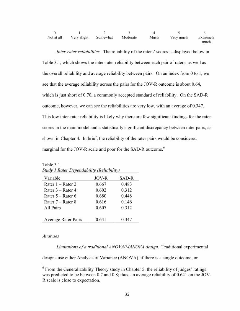
Inter-rater reliabilities. The reliability of the raters’ scores is displayed below in
Table 3.1, which shows the inter-rater reliability between each pair of raters, as well as
the overall reliability and average reliability between pairs. On an index from 0 to 1, we
see that the average reliability across the pairs for the JOV-R outcome is about 0.64,
which is just short of 0.70, a commonly accepted standard of reliability. On the SAD-R
outcome, however, we can see the reliabilities are very low, with an average of 0.347.
This low inter-rater reliability is likely why there are few significant findings for the rater
scores in the main model and a statistically significant discrepancy between rater pairs, as
shown in Chapter 4. In brief, the reliability of the rater pairs would be considered
marginal for the JOV-R scale and poor for the SAD-R outcome.6
Table 3.1 Study 1 Rater Dependability (Reliability)
Variable JOV-R SAD-R Rater 1 – Rater 2 0.667 0.483 Rater 3 – Rater 4 0.602 0.312 Rater 5 – Rater 6 0.680 0.448 Rater 7 – Rater 8 0.616 0.146 All Pairs 0.607 0.312
Average Rater Pairs 0.641 0.347
Analyses
Limitations of a traditional ANOVA/MANOVA design. Traditional experimental
designs use either Analysis of Variance (ANOVA), if there is a single outcome, or 6 From the Generalizability Theory study in Chapter 5, the reliability of judges’ ratings was predicted to be between 0.7 and 0.8; thus, an average reliability of 0.641 on the JOV-R scale is close to expectation.

33
Multivariate Analysis of Variance (MANOVA), if there are two or more outcomes.
Participants’ scores on the personality scale measuring general tendency towards
happiness/sadness (SHS) would be used to break the participants into three groups: 1)
those with a low score on the SHS (habitually sad); 2) those with a medium score on the
SHS (affectively neutral); and 3) those with a high score on the SHS (habitually happy).
Thus, the ANOVA/MANOVA would investigate the difference in emotional contagion
between groups distinguished by differences in trait-based happiness/sadness. One of the
disadvantages of this approach, however, is that need to split the participants into three
groups based on artificial cutoffs in their SHS score in order to implement the
comparative analysis between target conditions.
A second limitation of the traditional ANOVA/MANOVA approach is its
inability to handle individuals with partial data (i.e., where some observations may be
missing). Subjects with any missing data are simply dropped, which is known as listwise
deletion. Because this approach assumes missing cases are missing completely at
random (MCAR), which is typically only the case when a random sample is drawn from
a population, it will lead to biased model estimates in almost all situations (Hox, 2010).
A third limitation of this approach is the inability to incorporate data on
discrepancies due to raters, occasions of measurement, or their interaction directly into
the model, since this information is nested within the individual participants in the model
(Hox, 2010). In the ANOVA or MANOVA approach, this would require averaging data
on raters and occasions after they evaluated the recordings; that is, the information on
each individual participant compiled from raters over occasions would be averaged and
used along with the participants’ self-reports as the outcome measures in separate

34
ANOVAs, or analyzed together in a MANOVA, to see if the data supported the main
effect of target condition by comparing the means for the outcome variables, i.e. the
mean ratings by self-report and judges’ ratings for participants who watched the video
clip of either positive or negative emotion.
Mixed modeling approach. As discussed below, the traditional
ANOVA/MANOVA design was replaced with a mixed (or random coefficients) design,
which is a type of multilevel model where repeated measurements (e.g., occasions) and
rater assessments are nested within individuals. In its simplest form, this mixed model
represents a type of two-level model where rater assessments compiled over one or more
occasions are nested within individuals at Level 1 (within subjects), while the conditions
having to do with the experiment, as well as any other covariates, are entered as Level 2
(between subjects) data. Use of this sophisticated multivariate and multilevel model
thereby negates the need to justify artificial groupings in the data based on arbitrary cut-
offs on the SHS measure.
There are a number of advantages for specifying the analyses in this manner.
Most important for this study is the ability to include individuals with partial data in the
analyses. In contrast to ANOVA or MANOVA, which use listwise deletion of any
individuals with missing data, individuals with partial data can be included in the mixed
modeling approach. This analysis makes use of full information maximum likelihood
(FIML), which can provide efficient estimates in the presence of individuals with some
missing data. FIML estimation will lead to unbiased estimates when it can be assumed
that the data are missing at random (MAR); that is, if the probability of data being
missing on the outcome is related to missing data on a covariate, but not to subjects’

35
standing on the outcome, then the data are MAR (Hox, 2010). A second advantage for
purposes of this study is that the mixed modeling approach allows the incorporation of
error facets due to raters, occasions of measurement, or their interactions (as well as other
potential sources of error) directly into the model, which will provide more efficient
estimates of experimental conditions between subjects. A third advantage of the mixed
modeling approach is that it can facilitate the examination of multiple dependent
variables within one model (Hox, 2010).
Proposed model. The proposed models are presented in Figures 3.1 through 3.4.
From these figures, we can see the overall predictions for how happiness/sadness is
expected to influence susceptibility to emotional contagion, based on the two competing
hypotheses and using the different outcome measures (positive or negative affect, based
on either self-report or judges’ ratings). These predictions are expected to hold whether
happiness/sadness is measured as an enduring trait, as in Study 1, or as a transient mood,
as in Study 2 (to follow). The theoretical model assumes that there will be differences in
trait-based affect (i.e., a happy or sad personality) leading to different susceptibilities to
catching the positive or negative affect of others. Information about the measurement
qualities of the assessments is not shown in Figures 3.1 – 3.4, but is added to the within-
subjects part of the model (described in the next section). Figures 3.1 – 3.4 are continued
on the next page.

36
Figure 3.1. Addition theory: Positive affect as dependent variable
Figure 3.2. Addition theory: Negative affect as dependent variable
-‐2.5
-‐2
-‐1.5
-‐1
-‐0.5
0
0.5
1
1.5
2
2.5
Sad Person Neutral Person Happy Person
Positive Affect
Addition Theory: Positive Affect as Dependent Variable
Happy video, addition Sad video, addition
-‐2.5
-‐2
-‐1.5
-‐1
-‐0.5
0
0.5
1
1.5
2
2.5
Sad Person Neutral Person Happy Person
Negative Affect
Addition Theory: Negative Affect as Dependent Variable
Happy video, addition Sad video, addition

37
Figure 3.3. Interaction theory: Positive affect as dependent variable
Figure 3.4. Interaction theory: Negative affect as dependent variable
-‐2.5
-‐2
-‐1.5
-‐1
-‐0.5
0
0.5
1
1.5
2
2.5
Sad Person Neutral Person Happy Person
Positive Affect
Interaction Theory: Positive Affect as Dependent Variable
Happy Video, interaction Sad Video, interaction
-‐2.5
-‐2
-‐1.5
-‐1
-‐0.5
0
0.5
1
1.5
2
2.5
Sad Person Neutral Person Happy Person
Negative Affect
Interaction Theory: Negative Affect as Dependent Variable
Happy Video, interaction Sad Video, interaction

38
Two-level models. As noted previously, mixed, or random coefficients, modeling
is appropriate in research situations where data are nested within individuals. For each
participant in the study, there is a measurement model nested within the individuals.
More specifically, in the final models, two raters provided information on participants’
responses on two occasions which also covered multiple items. Such designs, which
require individuals to assess participants under various conditions, have the potential to
introduce considerable measurement error, which should be considered in the analyses to
explain participant responses to the experimental stimuli. What was needed was a design
that would include possible variability due to various errors facets (e.g., raters, occasions,
interactions) as part of the analyses (Marcoulides, 1998).
These measurement facets were included in the model at Level 1 (where the
assessment information is nested within subjects). The Level 1 model to explain an
individual’s observed emotional score ( ) can be described as follows:
, (3.1)
where is the adjusted score for individual j on assessment i after adjusting for
possible discrepancies due to rater differences, the occasion they are assessing, and
possible rater*occasion interactions, and represents residual variability in assessing
each individual’s emotional response.7 Level 1 (the within-group level) estimates are
presented in a log odds metric, since the outcome variable, i.e., the rater’s score, is
measured on an ordinal scale (i.e., 0 to 6).
7 Note that “items” were not included as a measurement facet in the main model. This decision was made based upon the preliminary Generalizability Theory study discussed in Chapter 5.
1ijY
1 0 1 2 3 *ij j ij ij ij ij ijY rater occasion rater occasion eβ β β β= + + + +
0 jβ
eij

39
At Level 2, the experimental condition (i.e., whether the person was watching a
happy or sad video) was added to the model, along with the emotional contagion score,
the subjective happiness score, the interaction between condition and subjective
happiness (to test between the addition and interaction theories), as well as demographic
controls for gender and age:
0 00 01 02 03
04 05 06 0* ,j j j j
j j j j j
condition emotcont subhappysubhappy condition female age u
β γ γ γ γ
γ γ γ
= + + + +
+ + + (3.2)
where is the intercept representing the average score when watching the happy video
(coded 0) and represents the change in the average score due to watching the other
condition (i.e., the sad video), 02 06γ γ− represent the coefficients for the other between-
subjects predictors, and represents the random component, that is, variability in
predicting the scores on the dependent variable across individuals. Through substitution
of Eq. 3.2 into 3.1, the combined equation representing the within-subject and between-
subject variables is as follows:
00 01 02 03
04 05 06
10 20 30 0
*
* .
ij j j j
j j j j
ij ij ij ij j ij
Y condition emotcont subhappysubhappy condition female agerater occasion rater occasion u e
γ γ γ γ
γ γ γ
γ γ γ
= + + + +
+ + +
+ + + + (3.3)
The mixed-model approach also facilitates the specification of other relationships
either within or between individuals. In this case, a second model can be specified
between-individuals. This second equation considers the self-report measure ( ) as the
between-subjects outcome:
00γ
01γ
0 ju
1 jY

40
β0 j = γ00(1) +γ01(1)condition j +γ02(1)emotcont j +γ03(1)subhappy j +
γ04(1)subhappy j *condition j +γ05(1) female j +γ06(1)age j +u0(1) j . (3.4)
As Eq. 3.4 indicates, there is no within-subjects model, since the outcome is a self-report
measure. Between-individual estimates for Eq. 3.3 and Eq. 3.4 are presented as
standardized (M = 0, SD = 1), since ordinal variables are treated as measured on an
underlying continuous scale at Level 2 in Mplus (Muthén & Muthén, 1998-2006), and
each participant’s self-report was measured on a continuous scale. The mixed model was
estimated using Mplus 6.12 (Muthén & Muthén, 2005), a statistical software package
which can be used to estimate multilevel models with outcomes measured on different
types of scales simultaneously. Figure 3.5 visually depicts the complete set of variables
and predicted interactions in the two-level model.

41
Figure 3.5. Two-level model for Study 1
Preliminary Analyses. Several preliminary analyses were conducted on the two
types of outcome variables—judges’ rating and self-report. The preliminary analysis for
judges’ ratings will be discussed in Chapter 5 (Method of Study 2). The preliminary
analysis for self-report data is discussed here, as Study 1 includes self-report measures as
both predictor and outcome variables.

42
In review, prior to watching the target video in the main experiment, participants
in Study 1 took a pre-experiment survey that included the Subjective Happiness Scale
(SHS), the Emotional Contagion Scale (ECS), and the Life Orientation Test-Revised
(LOT-R). After viewing the target video, participants took a post-experiment survey
including the Positive and Negative Affect Schedule (PANAS), and the Joviality and
Sadness scales from the extended version of the PANAS (PANAS-X). Collectively these
data will be referred to as the self-report database.
As the goal is to provide a preliminary test of the proposed relationships, it is
assumed that the available sample may not fully represent the population at large;
therefore, the results should not be extrapolated beyond this particular sample. A
preliminary step in the data analysis process was to use exploratory factory analysis to
improve the psychometric properties of the self-report data prior to testing the study’s
main hypotheses. More specifically, it is important to first ensure that the variables were
appropriately and reliably measured before the data is used in the main analysis to
examine the effects of the various experimental conditions on subjects’ responses.
Field (2009) identifies three purposes of factor analysis: 1) to understand the
structure of the latent variable(s) behind a set of variables; 2) to construct a scale to
measure an underlying variable; and 3) to reduce a data set to a more manageable size
while retaining as much of the original information as possible. In this study, principal
component analysis (PCA) was used for the latter purpose; that is, as a data reduction
method, rather than a theoretical approach, to weight the specific items defining their
proposed underlying constructs.

43
The goal was to create a single scale, or one “weighted” component, in which
each of the items is weighted according to the strength of its relationship to the
dimension. For example, merely adding three items together assumes that they contribute
equally to the dimension, i.e., they are given the same weight. However, in fact, one item
may be more strongly related to the dimension than the other two items and should be
given greater weight, which will yield a more accurate estimate than not accounting for
differences in the strength of the relationship between each item and the dimension. Each
item is allowed to contribute to the component through its weighted factor score, and the
researcher can then investigate how the reliability (Cronbach’s alpha) of the scale would
be affected by the removal of the item. This process reduces problems of
multicollinearity, as the correlated items are combined to form a factor.
To conduct the PCA, variables that are reverse scored on the original measures
were recoded (e.g., SHS4r in Table 3.2 is a reverse score “r” of item 4 in the Subjective
Happiness Scale) to positively correlate with the scales. Reliability analyses were then
conducted, and items whose deletion would most increase the reliability of the scale were
removed to adopt a minimum of α = 0.70 for each scale. See Tables 3.2 – 3.8 (continued
on the next page) for the resultant component matrices and reliability scores of each scale
used in Study 1 (and Study 2).

44
Table 3.2 Component Matrix of SHS Component
1 SHS2 .800 SHS3 .873 SHS4r .709
α = 0.70
Table 3.3 Component Matrix of ECS
Component 1
ECS1 .578 ECS2 .484 ECS3 .584 ECS4 .596 ECS5 .404 ECS6 .443 ECS7 .406 ECS8 .638 ECS9 .612 ECS10 .473 ECS11 .544 ECS12 .533 ECS13 .413 ECS14 .628 ECS15 .445
α = 0.81
Table 3.4 Component Matrix of LOTR Component
1 LOTR1 .552 LOTR3r .669 LOTR4 .749 LOTR7r .688 LOTR9r .702
α = 0.75
Table 3.5 Component Matrix of PA Scale (PANAS) Component
1 PA1 .755 PA2 .577 PA3 .638 PA4 .803 PA5 .857 PA6 .842 PA7 .808 PA8 .705 PA9 .782 PA10 .813
α = 0.92

45
Table 3.6 Component Matrix of NA Scale (PANAS) Component
1 NA1 .575 NA2 .513 NA3 .606 NA4 .388 NA5 .613 NA6 .438 NA7 .616 NA8 .617 NA9 .706 NA10 .579
α = 0.75
Table 3.7 Component Matrix of Joviality Scale (PANAS-X) Component
1 Happy1 .893 Happy2 .904 Happy3 .906 Happy4 .884 Happy5 .839
α = 0.93
Table 3.8 Component Matrix of Sadness Scale (PANAS-X) Component
1 Sad1 .850 Sad2 .810 Sad3 .729 Sad4 .706 Sad5 .767
α = 0.83
It is noted that one item was removed from the SHS (item 1) and one item was
removed from the LOTR (item 10), in addition to the filler items that should be excluded
from the scoring of the original LOTR scale (items 2, 5, 6, and 8). In sum, PCA was used

46
to create weighted factor scores (M = 0, SD = 1) for each variable that were then saved
into the database for use in the main analyses. The self-report measure, now “weighted”
in terms of each item’s contribution to the underlying construct, was then brought into the
main multilevel model at Level 2 (between subjects), where condition effects and other
between-subjects variables should be.
Another benefit to the PCA is the ability to identify the best performing outcome
measure of the four self-report scales (PA, NA, Joviality, Sadness). Overall, the positive
affect measures (PA and Joviality) had greater reliability (alphas) than the negative affect
scales (NA and Sadness). Indeed, we might select just the highest performing measure,
the Joviality scale (α = 0.93), for use as the self-report outcome variable in the main two-
level model. However, for consistency, it was desirable to keep a measure of negative
affect in the analysis as well. Therefore, both the Joviality and Sadness measures were
used as the self-report outcome variables, in addition to the JOV-R and SAD-R scores
from the judges’ ratings (see Chapter 5). While the collection of data on the full PANAS
was instructive, including the PA and NA scales as additional outcome measures in the
main model would be redundant, as the Joviality (α = 0.93) and Sadness (α = 0.83) scales
outperform the PA (α = 0.92) and NA scales (α = 0.75), respectively.

47
CHAPTER 4
RESULTS OF STUDY 1: ENDURING AFFECT AND EMOTIONAL CONTAGION
Descriptive Statistics
The descriptive results of the self-report data are presented in Table 4.1 below.
As the Joviality and Sadness scales were transformed into factor scores (see Chapter 3),
the scale means (M) and standard deviations (SD) for the two conditions are standardized.
The means for the two conditions reflect how far each group’s mean deviates from the
sample mean (M = 0.0, SD = 1). For example, considering the Joviality scale,
participants who watched the sad target video, as expected, reported lower positive affect
(n = 81, M = -0.388, SD = 0.838) at the end of the experiment than participants in the
Happy condition (n = 77, M = 0.350, SD = 1.037), indicating a statistically significant
difference in means of 0.738 (t(156) = 4.866, p < .001), i.e., a considerable difference in
perceptions between the two experimental conditions. In contrast, when the outcome was
measured by self-report on the Sadness scale, participants in Happy condition reported
less sadness than average (n = 77, M = -0.186, SD = 0.962); however, those exposed to
the sad stimuli did as well (n = 81, M = -0.062, SD = 0.800). The overall difference in
standardized means between the two conditions was much smaller on the Sadness scale
(0.124) than the Joviality scale (0.738), and non-significant.
Table 4.1 Descriptive Statistics for Self-Report by Factor Scores Within Conditions by Joviality and Sadness Scales
Joviality
Sadness Condition n M SD T-Test M SD T-Test
Happy Stimuli 77 0.350 1.037 4.866**
-0.189 0.963 -0.894 Sad Stimuli 81 -0.388 0.838
-0.062 0.800
Note. **p < .001

48
The descriptive results of the data from the judges’ ratings are shown in Table 4.2,
which presents the means and standard deviations of the JOV-R and SAD-R ratings on a
7-point ordinal scale. From the table, we get a sense that the overall scoring of emotion
was relatively low, as all the means are close to zero, suggesting that the raters evaluated
the participants as having very little visible signs of emotion. Overall, while not
definitive, since both differences are small and non-significant, the results in Table 4.2
imply that raters identified slightly more expressed emotion regarding the sad stimuli for
both scales (i.e., the means on both the JOV-R and SAD-R scales are higher sad stimuli).
Table 4.2 also suggests that the JOV-R scale provided more variability (higher standard
deviations) in terms of emotional response, which was interpreted as supportive evidence
for emphasizing the JOV-R scale to determine the effects of the various experimental
conditions on participants.
Table 4.2 Descriptive Statistics for Judges’ Ratings on an Ordinal Scale Within Conditions by JOV-R and SAD-R Items
JOV-R
SAD-R Condition n M SD T-Test M SD T-Test
Happy Stimuli 77 0.849 1.402 1.100
1.039 1.019 -1.694 Sad Stimuli 81 0.767 1.538
-0.062 1.147
Summary of Two-Level Model
The proposed model as tested is presented in Figure 4.1 (continued on the next
page). Between subjects, there are two between-subjects (Level 2) outcomes in the
model. The first is the judges’ score (on the JOV-R or SAD-R scales) and the second is
the subjects’ self-report factor score (on the Joviality or Sadness scales). Within subjects

49
(Level 1), only the judges’ score is shown, since this outcome is dependent on ratings
over two occasions.
Figure 4.1. Proposed model for Study 1.
Two-Level Model Results with Positive Affect Outcome Measures
In Table 4.3, the results of the main two-level model with positive affect outcome
measures are presented. Between subjects, the JOV-R score represents judges’ ordinal
ratings of subjects’ displayed emotion. The second outcome is subjects’ self-report factor
score on the Happiness scale. Both are standardized (M = 0, SD = 1) between subjects.
The reference condition for both outcomes is the Happy condition (watching the happy
target video).

50
Table 4.3 Two-Level Model Estimates on the JOV-R Scale
Variables Estimate SE T-Test Sig.
Between Subjects (N = 158) Happiness Scorea Sad Target -0.063 0.079 -0.795 0.322 Emotional Contagion 0.061 0.110 0.553 0.612 Subjective Happiness 0.170 0.289 0.591 0.494 Subjective Happiness*Sad Target -0.098 0.291 -0.338 0.735 Age -0.063 0.060 -1.047 0.295 Female -0.020 0.095 -0.216 0.829 Within Subjectsb Occasions 0.018 0.241 0.076 0.939 Rater Teams 0.059 0.355 0.167 0.867 Occasions x Rater Teams -0.400 0.352 -1.137 0.256 Between Subjectsa Self-Report Happiness Intercept 1.171 0.464 2.524 0.012 Sad Target -0.365 0.068 -5.356 0.000 Emotional Contagion 0.136 0.076 1.780 0.075 Subjective Happiness 0.666 0.230 2.901 0.004 Subjective Happiness*Sad Target -0.379 0.214 -1.770 0.077 Age 0.015 0.085 0.173 0.836 Female -0.109 0.073 -1.488 0.137 Level 2 variance (Score) 10.882 1.883 5.778 0.000 Level 2 variance (Self-Report) 0.727 0.081 9.014 0.000 Correlation 0.091 0.087 1.046 0.295 Log likelihood -1620.5 Free parameters 25
Note. a Between-subject estimates are standardized coefficients; b Within-subject estimates are log odds coefficients; thresholds not shown.
For the judges’ ordinal outcome, we can see that participants in the Sad condition
were evaluated as expressing less happiness on average (-0.063) than the participants
who watched the happy target video when controlling for other variables in the model;
this relationship is in the right direction but was not significant (p = .322). Emotional
contagion, as measured by the Emotional Contagion Scale (ECS), had an estimated effect
on JOV-R judges’ ratings in the predicted direction (though non-significant); that is, a

51
one standard deviation increase on the ECS, reflecting higher susceptibility to emotional
contagion, would predict a .061 increase in emotion as measured by the JOV-R scale.
Similarly, enduring affect, as measured by the Subjective Happiness Scale (SHS), also
influenced JOV-R scores in the predicted direction—according to both the addition and
interaction hypotheses, higher levels of trait-based happiness would predict higher
susceptibility to picking up happy emotion. Although the relationship between subjective
happiness and judges’ ratings of participant happiness was in the predicted direction
( = .170), it was non-significant (p = .494). The interaction between SHS and condition
(i.e., the Sad Target) was also not significant ( = -0.098, p = .735).
While the data by judges’ ratings yielded no significant results, turning to the self-
report factor scores (for Joviality), Table 4.3 suggests that participants watching the sad
target video reported significantly lower self-report happiness scores ( = -0.365,
p < .001) compared to their peers watching the happy target video. This finding suggests
that participants in the Sad condition reported their happiness level on the Joviality scale
to be 0.37 of a standard deviation less than those who watched the Happy target video.
Importantly, an increase in subjective happiness of one standard deviation would result in
a 0.666 SD increase in self-reported happiness (on the Joviality scale) when assigned to
the Happy condition (p = .004), controlling for the other variables in the model. At
α = .10, the interaction between condition and SHS is significant ( = -.379, p = .077).
These findings are graphically depicted in Figure 5.2 (continued on the next page).
γ
γ
γ
γ

52
Figure 4.2. Results of Study 1 with the outcome measured on the Joviality scale.
Considering the other covariates in the model, a one SD increase on the ECS
would result in an increase of 0.136 (p = .075) in observed emotion; this finding is
significant at the more lenient alpha level of .10. The influence of demographic
characteristics such as age and gender was not significantly related to the outcome on
either measurement scale.
Importantly, the non-significance of the Level 1 (within subjects) variables for the
JOV-R score in Table 4.3 suggests little possible impact of differences between occasions
measured (p = .939), raters (p = .867), or their interaction (p = .256); i.e., variability on
these components is not significantly predicting the outcome measured on the JOV-R
scale. We can also note that the JOV-R and Joviality outcome measures are positively,

53
but non-significantly correlated (r = 0.091, p = .295), suggesting that the rater scoring
and participants’ self reports may be tapping into different constructs (as will be
discussed further in Chapter 7).
Two-level Model Results With Negative Affect Outcome Measures
Table 4.4 (continued on the next page) presents the results of the main model with
judges’ scores on the SAD-R scale and the self-report Sadness scale used as outcome
measures. Again, the baseline comparison is to the Happy condition. In contrast to the
data collected on the positive affect measures, there were no significant relationships
found on either the SAD-R or Sadness scales, even at the more lenient alpha of α = .10.
Again, we find a non-significant, small correlation between the SAD-R and
Sadness scales (r = -0.025, p = .896), suggesting that raters’ scoring and participants’ self
reports are not measuring the same thing (see Chapter 7). None of the Level 1 (within
subjects) variables contributed significant variance to these estimates, suggesting that
raters, occasions, and the interaction between these terms did not affect judges’ scores on
the SAD-R scale.

54
Table 4.4 Two-Level Model Estimates on the SAD-R Scale
Variables Estimate SE T-Test Sig. Between Subjects (N = 158) Sadness Scorea Sad Target -0.068 0.087 -0.776 0.438 Emotional Contagion 0.062 0.110 0.561 0.575 Subjective Happiness 0.165 0.289 0.571 0.586 Subjective Happiness*Sad Target -0.090 0.291 -0.308 0.758 Age -0.058 0.061 -0.952 0.341 Female -0.025 0.095 -0.261 0.794 Within Subjectsb Occasions -0.170 0.208 -0.816 0.414 Rater Teams -0.244 0.981 -0.248 0.804 Occasions x Rater Teams 0.071 0.626 0.114 0.910 Between Subjectsa Self-Report Sadness Intercept -0.205 0.425 -0.482 0.630 Sad Target 0.102 0.081 1.259 0.208 Emotional Contagion 0.149 0.138 1.085 0.278 Subjective Happiness -0.058 0.240 -0.244 0.807 Subjective Happiness*Sad Target -0.111 0.241 -0.460 0.645 Age -0.054 0.041 -1.329 0.184 Female -0.015 0.076 -0.198 0.843 Level 2 variance (Score) 10.893 1.125 5.237 0.000 Level 2 variance (Self-Report) 0.745 0.188 3.962 0.000 Correlation -0.025 0.190 0.130 0.896 Log likelihood -1621.0 Free parameters 25
Note. a Between-subject estimates are standardized coefficients; b Within-subject estimates are log odds coefficients; thresholds not shown.

55
CHAPTER 5
METHOD OF STUDY 2: TRANSIENT AFFECT AND EMOTIONAL CONTAGION
In Study 2 we plan to test Hypothesis 2: Transient affect, i.e., a happy or sad
mood state, will affect susceptibility to catching either positive or negative emotions. We
will explore which of the two theories—the addition theory, which states that participants
will be most likely to catch emotions that are congruent with current affect, or the
interaction theory, which states that the happier participants are, the more likely they will
be to catch others’ emotions—is the best fit for the data.
Participants
The participant population consisted primarily of undergraduate students from the
University of Hawai‘i at Mānoa (UH) who were recruited from courses in the social
sciences. These students also recruited their family and friends, for a total of 182
participants (37% male, 63% female) whose ages ranged from 18 to 72 years (M = 23
years). As participants were mainly recruited from UH, the sample was representative of
the demography of the university in categories such as education level and race/ethnicity
(21.4% Caucasian; 20.3% Japanese; 14.8% Filipino; less than 10% African, American
Indian, Chinese, Hawaiian, Hispanic, Korean, Middle Eastern, Pacific Islander,
Indian/South Asian, Other Asian, and Other/Choose Not to Disclose).
Participants signed up on an electronic spreadsheet, which randomly assigned
them to one of six conditions by combination of mood manipulation (positive, neutral, or
negative mood induction procedure) and stimuli, which was designed to induce positive
or negative emotion. Following the experiment, participants were fully debriefed as to
the full purpose of the study—to see whether people tend to catch other people’s

56
emotions and if so, what impact a person’s transient mood has on his or her susceptibility
to such contagion.
Debriefing included the disclosure that their facial expressions to the video clips
of positive and negative emotional displays were recorded to investigate whether outside
ratings of their emotion would correspond to their own self-report, thus giving a more
complete assessment of the participant’s emotional state. Upon debriefing, participants
were given the opportunity to delete the recording, an option no participant selected.
Participants were only allowed to participate if they were at least 18 years old.
Students enrolled in certain courses at UH received extra-credit for their participation,
however no other compensation was offered to participants in the study.
Measures
Two surveys (pre and post-experiment) were administered to the sample
population via SurveyMonkey.com, an online survey and questionnaire tool of increasing
popularity (Evans et al., 2009). All surveys were administered by Research Assistants
(RAs) in the Hatfield Lab and were comprised of pre-tested measures with demonstrated
validity and reliability. The measures included in both the pre- and post-experiment
surveys are listed below and then described in further detail.
Pre-experiment: • Demographic information
Post-experiment: • Positive and Negative Affect Schedule,
PANAS (Watson et al., 1988) • Joviality and Sadness scales from the
Positive and Negative Affect Schedule – Extended Form, PANAS-X (Watson & Clark, 1999)
Positive and Negative Affect Schedule (PANAS). In the Positive and Negative
Affect Schedule (PANAS), respondents are presented with words describing positive
moods (e.g., excited) and negative moods (e.g., hostile), and asked to rate each according

57
to the extent to which it describes them. As noted by Shiota and colleagues (2006),
critics of the PANAS contend that several of the items on the tool are not actually
emotions (e.g., determined, alert), and that several important positive emotions for
wellbeing are absent from the scale (e.g., love, contentment, amusement).
A widely used scale across psychological and physical activity research, the
PANAS thus consists of two 10-item mood scales for Positive Affect (PA) and Negative
Affect (NA) that are shown to be highly internally consistent (0.86 – 0.90), largely
uncorrelated, and stable at appropriate levels over a two-month time period (Watson et
al., 1988). The PANAS allows for temporal variations in the assessment; researchers
may choose whether to ask for a rating “right now,” “over the past few days,” or simply
“in general.” In this study, participants were asked to indicate to what extent they felt the
mood in question “right now, at this present moment.”
Responses to the 20 items were measured using a seven-point response scale
ranging from 0 (not at all) to 6 (extremely much). Ratings were then summed separately
across the two scales, allowing positive affectivity to be calculated independent of
negative affectivity, e.g., people can be high in both positive affect and negative affect.
Scores on both scales could range from 10 to 50, with low scores indicating low positive
or negative affect and high scores indicating high PA or NA (PA, α = .92; NA, α = .75).
Joviality and Sadness Scales from the Positive and Negative Affect Schedule—
Extended Form (PANAS-X). Positive affect and negative affect have reliably emerged as
the dominant dimensions of emotional experience across diverse descriptor sets, time
frames, response formats, languages, and cultures (see Almagor & Ben-Porath, 1989;
Mayer & Gaschke, 1988; Meyer & Shack, 1989; Watson et al., 1988; Watson &

58
Tellegen, 1999). Nevertheless, although PA and NA account for most of the variance in
self-rated affect, Watson and Clark (1999) found that specific emotional states can also
be identified within these overarching dimensions. They proposed a hierarchical
taxonomic scheme in which PA and NA describe the valence of 11 correlated, yet
ultimately distinguishable affective states: Fear, Sadness, Guilt, Hostility, Shyness,
Fatigue, Surprise, Joviality, Self-Assurance, Attentiveness, and Serenity.
In this study, the Joviality (Happiness) and Sadness scales were clearly the most
relevant to the research questions and hypotheses. These two scales were selected to
supplement the original 20 items from the PANAS on the post-experiment survey. The
original Joviality scale from the PANAS-X includes eight items (happy, cheerful, joyful,
excited, enthusiastic, lively, energetic, delighted), of which the latter three had the
weakest varimax-rotated factor loadings, with lively and energetic loading onto separate
factors as well (Watson & Clark, 1999). Thus, the three weakest performing items were
excluded to form a five-item measure commensurate with the five-item Sadness scale.
Scores on the Joviality and Sadness scales could range from 5 to 25, with low scores
indicating low happiness/sadness, and high scores indicating high happiness/sadness
(Joviality, α = .93; Sadness, α = .83).
Mood Induction
After completing the pre-experiment survey (demographic information only),
participants engaged in a task designed to induce temporary affect. Imagery tasks were
used as Mood Induction Procedures (MIPs), a form of affect induction common in studies
involving laboratory mood manipulations (e.g., Delp & Sackeim, 1987; Larsen & Sinnett,
1991; Salovey & Birnbaum, 1989). This MIP has also been referred to as the

59
autobiographical recollections method (Goodwin & Williams, 1982) or as self-generated
imagery (Singer & Salovey, 1988).
Choosing a MIP can be a difficult task, as the literature on the effectiveness of
MIPs is varied and conflicted (Coan & Allen, 2007; Philippot, 1993). One of the most
common procedures, the Velten technique (1968), instructs the participant to read 60 self-
referential statements that begin neutrally and become progressively more elated or
depressed in content, depending on the particular induction. The technique has spawned
several modifications (see Larsen & Sinnett, 1991; Pignatiello, Camp, & Rasar, 1986;
Sinclair, Mark, Enzle, Borkovec, & Cumbleton, 1994) and continues to receive support
(Finegan & Seligman, 1995) despite criticism for inducing demand characteristics
(Buchwald, Strack, & Coyne, 1981; Polivy & Doyle, 1980). The Velten technique was
considered for this study but eschewed for considerations of time (the procedure takes
around 20 minutes) and efficacy.
Other MIPs considered include written procedures (Baker & Gutterfreund, 1993),
listening to music (Pignatiello et al., 1986; Västfjäll, 2001), and watching film clips8
(Hewig et al., 2005). The imagery task was eventually selected after a review of several
meta-analyses of MIP effectiveness and validity (see Gerrards‐Hesse, Spies, & Hesse,
1994; Larsen & Sinnett, 1991; Westermann, Spies, Stahl, & Hesse, 1996), which
suggested that the imagery task would most efficiently induce stable and reasonably
intense moods for the purpose of this study.
8 The film clip MIP is evidently similar to the experimental design of the study, i.e., to have participants watch a clip of either positive or negative emotion. It may be that the film clip MIP works precisely through the process of emotional contagion, as the viewer “catches” the emotion of the target.
60
Using a between-subjects design, participants were manipulated into one of three
affect conditions: positive, neutral, or negative. Three videos were created and put on
YouTube to allow the video to be embedded within the online survey, along with the
target video of either positive or negative emotion (see the following section on Stimuli).
The MIP videos involved written directions that were shown on the screen while they
were also read out loud by an actor chosen for having a neutral and professional voice.
Mood-congruent music was played in the background of each video to further enhance
the affect induction (Pignatiello et al., 1986; Västfjäll, 2001). The total length of each
mood-induction video was approximately three minutes.
Each condition involved having participants read (and listen to) two written
scenarios designed to induce the intended affect. Participants were asked to create a
vivid image of themselves in each situation described by the scenarios. Before being
guided through the affective scenarios, participants were told that they might be asked to
recall parts of the scenarios later and that their memory would be improved if they could
actually “get into the feeling” of each scene as they read and imagined it. Specifically,
participants were instructed to do the following:
Imagine the situation as vividly as you can. Picture the event happening to
you. Try to imagine all the details of the situation. Picture in your
“mind's eye” the surroundings as clearly as possible. See the people or
objects; hear the sounds; experience the event happening to you. Think
the thoughts you would actually think in this situation. Feel the same
feelings you would feel in this situation. Let yourself react as if you were
actually there.

61
After this preparation, the participant was guided through a pair of scenarios of
the same hedonic tone depending on the experimental condition, with one minute
following each statement in which he/she was asked to “Please concentrate on this scene,
relax, close your eyes, and imagine being in that situation until you hear my voice again.”
The scenarios used in each condition are as follows:
1. Positive
a. You have won $50,000 in a lottery and you are now taking a vacation
to your dream destination.
b. Now imagine that you are feeling relaxed and healthy as you take a
walk on a beautiful day. You find a $5 bill on the ground.
2. Neutral
a. You go to the supermarket.
b. You go on a walk.
3. Negative
a. A close friend of yours gets into a car accident. You go to the hospital
and find out that he/she has just died an hour ago and you didn’t get
the chance to say goodbye.
b. You are going through a breakup with a significant other that you have
been with for a while and you hear a sad song on the radio that
reminds you of him/her.
Manipulation check. Following the MIP, participants were asked if they
experienced any emotions, memories, or physical sensations. If emotions were reported,
their intensity was rated on a 0 to 8 scale, with 8 equivalent to the strongest experience of
62
that emotion in the participant’s entire life. Participants were also asked to rate the
difficulty of engaging or “getting into” the MIP using a 0 to 8 scale. This manipulation
check was used successfully in a study by Levenson, Carstensen, Friesen and Ekman
(1991) to assess the efficacy of a relived emotion task.
Stimuli
Stimuli consisted of two videos, or targets, commensurate with the two groups of
experimental conditions—whether the participant was exposed to a Happy or Sad
emotion. The clip of positive emotion (Happy Target) showed the response to David
Freese’s homerun to win Game 6 of the 2011 Major League Baseball World Series, i.e.,
the ensuing celebration by the Saint Louis Cardinals and their fans—their joyous faces,
expressions of exultation and delight, and joyous postures. The clip of negative emotion
(Sad Target) focused on the sad and disappointed reactions by the Texas Rangers and
their fans; e.g., mournful faces, agonized moans, and hunched postures.9 Both clips were
approximately two minutes long.
Design
Participants were randomly assigned to one of six conditions through the
interaction of three MIPs and two stimuli. Participants were first manipulated into one of
three moods using a guided imagery task previously demonstrated to effectively induce a
happy, neutral, or negative mood (Larsen & Ketelaar, 1991). They were later asked to
watch a video clip of a target displaying either positive or negative emotion. The
resultant MIP/stimuli combinations were as follows: 1) Positive MIP / Happy Target; 2)
9 To control for gender differences in reaction to the sports videos, gender will also be tested in the model as a covariate. The issue of gender-specific reaction to emotional stimuli is a different problem beyond the scope of this study.

63
Neutral MIP / Happy Target; 3) Negative MIP / Happy Target; 4) Positive MIP / Sad
Target; 5) Neutral MIP / Sad Target; and 6) Negative MIP / Sad Target. Both MIP
condition and Target condition are between-subjects factors.
As in Study 1, the outcome was measured in the following ways: 1) Self-report
by the PANAS, which yields a score of Positive Affect (PA) and Negative Affect (NA),
on the post-experiment survey; 2) Self-report by the Joviality and Sadness scales from the
extended PANAS-X, on the post-experiment survey; and 3) Two raters trained using
either the Micro Expression Training Tool (METT) or the Subtle Expression Training
Tool (SETT)10 evaluated two snapshots of the participant’s facial expressions using an
abridged version of the Joviality and Sadness scales of the PANAS-X. Thus, we had a
total of six outcome measures: four self-report scales (PA, NA, Joviality, and Sadness),
and two scores by raters. Since the raters used abbreviated versions of the Joviality and
Sadness scales, further discussion of the scales used by the judges on the rating task will
be referred to as JOV-R and SAD-R, to differentiate these variables from the self-report
measures of Joviality and Sadness.
Considering the latter outcome measure (judges’ ratings), the use of multiple
raters, items, and occasions of assessment introduces a margin of error. Generalizability
theory (G theory; Shavelson & Webb, 1991) is one approach that considers multiple
errors in an evaluation design. A G theory preliminary study was conducted (see the
Analysis section) to consider a number of different scenarios before deciding on the
optimum combination of raters, items, and occasions that would yield data at an
acceptable level of reliability.
10 Again, sincere appreciation is extended to the Paul Ekman Group, LLC, for use of the METT and SETT programs.

64
Procedure
Six different electronic forms were used for the study (Forms C – H, as Forms A
– B were used for Study 1), depending on the MIP / Target video condition. Each form
included: 1) the pre-experiment survey; 2) the MIP video (inducing Positive, Neutral, or
Negative affect); 3) the target video; and 4) the post-experiment survey. The RAs were
blind to which target video was included in each form, to contain experimenter effects.
Additionally, participants watched the video with headphones on, so that the RA was
unable to hear the video and could not respond to it along with the participant.
6. Pre-experiment survey. The participant was welcomed into the lab by an RA
and seated in front of a Mac laptop. The consent form was already loaded on
the screen as the preliminary page of the pre-experiment survey. Participants
were informed of the intent to possibly record their facial expressions in the
consent form. The pre-experiment survey took under four minutes and ended
on a page instructing the participant to wait for the RA to input a code:
“Please STOP here. Please inform the research assistant that you have
completed this survey.”
7. Mood Priming and Manipulation check. The participant then watched a video
to induce positive, neutral, or negative affect, depending on the assigned
condition. The MIP videos were each approximately three minutes long, and
were followed by two survey questions designed to assess the effectiveness of
the mood induction. Data yielded from this manipulation check were not used
in the main analyses, but will be discussed in a separate analysis of the
efficacy of the mood induction procedure.

65
8. Experiment. After the participant completed the pre-experiment survey, when
the RA entered the “code,” he or she surreptitiously started the Photo Booth11
program as well. As noted above, the RA was blind to which condition the
participant was in, knowing only which form (C – H) the participant was
assigned to. After starting the video, the RA sat in a corner, able to answer
any questions that came up by the participant, but out of his/her viewing
radius. The participant watched the target video while his/her facial
expressions were simultaneously recorded.
9. Post-experiment survey. After watching the stimuli, the participant took the
post-experiment survey comprised of the PANAS and the Joviality and
Sadness scales from the PANAS-X. The post-experiment survey ended on a
page that signified completion of the study. The participant was instructed to
print this page in order to receive extra credit for his/her participation.
10. Debriefing. The participant was then informed of the full purpose of the
study—to assess whether emotional contagion is affected by transient affect—
and given the opportunity to review the recording of his/her facial expressions
and delete it if desired (which no participant chose to do).
11. Rating recordings. The recordings of the participants’ facial expressions were
judged by outside raters and these scores were used as an outcome variable in
addition to the self-report measures.
11 Photo Booth is a small software application by Apple Inc. for taking photos and videos with a camera built into the Mac. Other than a small green light at the top of the laptop, participants are not able to see themselves being recorded, minimizing the potential for distractions and induced participant effects.
66
a. A set of eight RAs was trained in recognizing emotion with the either the
Micro Expression Training Tool (METT) or the Subtle Expression
Training Tool (SETT), both administered online. The METT/SETT takes
approximately one hour to complete, and trainees receive pre- and post-
test scores of their accuracy in reading emotional cues. All RAs received
over 80% accuracy on the post-test in order to participate in coding.
b. The entire set of 34 videos from both Studies 1 and 2 was divided amongst
four pairs of raters; thus, each pair rated the same 85 videos (for reliability
analysis between raters), i.e., each participant’s video was independently
coded by two raters.
c. For each video coded, the RA watched the entire recording of the
participant one time through, and then on the second viewing stopped the
video at the two points or “occasions” at which the participant expressed
the most emotion.
d. These two occasions were then rated using three items from the Joviality
and Sadness scales of the PANAS-X (see the following section for further
detail on the items selected). Raters were instructed as follows:
This scale consists of a number of words and phrases that describe
different feelings and emotions. Read each item and then indicate
to what extent you think the person in the snapshot feels this way
at that moment.
Items were evaluated on the following metric:
0 1 2 3 4 5 6 Not at all Very slight Somewhat Moderate Much Very much Extremely
much

67
Inter-rater reliabilities. The reliability of the raters’ scores is displayed below in
Table 5.1, which shows the inter-rater reliability between each pair of raters, as well as
the overall reliability and average reliability between pairs. While the reliability is
relatively low for the judges’ ratings (i.e., 0.659 on the JOV-R outcome and 0.285 on the
SAD-R scale), one of the reasons that the rating data was included at Level 1 in the main
multi-level model was to show that there are no “statistically significant” differences in
the discrepancies between pairs of judges. In brief, the reliability of the rater pairs would
be considered marginal for the JOV-R scale and poor for the SAD-R outcome, and the
low inter-rater reliability is likely why there are few significant findings for the rater
scores in the main model, as shown in Chapter 6. As discussed in the following analysis
of judges’ ratings using generalizability theory, the reliability of judges’ ratings was
predicted to be between 0.7 and 0.8; thus, an average reliability of 0.659 on the JOV-R
scale is close to expectation.
Table 5.1 Study 2 Rater Dependability (Reliability)
Variable JOV-R -R Rater1 – Rater 2 0.573 0.488 Rater 3 – Rater 4 0.692 0.285 Rater 5 – Rater 6 0.608 0.267 Rater 7 – Rater 8 0.764 0.099 All Pairs 0.626 0.155
Average Rater Pairs 0.659 0.285
Analyses
Judges’ ratings. Within individuals, preliminary analyses focused on establishing
the minimum number of raters, items (from the Joviality and Sadness scales of the

68
PANAS-X), and occasions necessary to ensure reliable information could be gathered
relative to subject responses to the video stimuli. In this case, there are several possible
sources of error that could bias the analyses of differences between individuals due to the
experimental conditions. These facets included variability due to raters, variability due to
the items of the measures, and the number of occasions being assessed.
One useful psychometric model for assessing reliability, among other uses, is
referred to as generalizability (G) theory (Cronbach, Glesser, Nanda, & Rajaratnam,
1972; Marcoulides, 1996, 1998). G theory presents multifaceted sources of variability in
a measurement, including multiple sources of error variability (Shavelson & Webb,
1991). This ability to account for multiple sources of error allows us to identify how
individual differences between raters affected the reliability of their evaluations of the
participants’ facial displays of emotion (similar to Cronbach’s alpha).
The goal of a G study is to separate the variability in the evaluation object (i.e.,
the rating of emotion), into a variety of different sources, or variance components.
Typically, variance components may include variability due to differences among the
objects being evaluated, the raters assessing the objects, the type of instrumentation being
used, the number of occasions on which the objects are assessed, as well as various
interactions between these components (Marcoulides & Heck, 1992). A G study usually
involves a preliminary study using a subset of information (i.e., a pilot study) that can
strengthen the overall evaluation design by identifying aspects of the assessment
procedures that can be changed to reduce error.
In this analysis, it is assumed that an observed score (i.e., a rating of the emotion
in the participant’s facial expression) represents an evaluation of a sample of items made

69
at a given point in time, and if a different set of items were used, the observed score
would be somewhat different (Shavelson & Webb, 1991). As it is seldom practical or
attainable to obtain data on all possible items (Cronbach et al., 1972), the evaluation must
be generalized from a limited sample of items to the universe of all possible observations.
G theory allows us to ask how well the raters are performing over the number of
items they are using in the assessment, the number of occasions when the participants’
facial expressions are evaluated, and whether there is any interaction between any of
these components. We first decompose the raters’ scores into a universe score (i.e., the
score over all combinations of raters, items, and occasions) and variance components for
any other errors associated with the measurement study (Marcoulides, 1998). After
identifying major sources of error, a generalizability coefficient ( ) can be estimated to
describe the dependability of generalizing from an observed score based on the sample
observations to the mean score derived from all acceptable observations (Cronbach et al.,
1972; Heck, Johnsrud, & Rosser, 2000).
G theory model. In this case, we will use the raters’ score (0 – 6) as the main
object of assessment, decomposing the ratings into components that describes differences
in observations (referred to as the universe score) versus any variance in scores due to
errors introduced by the number of raters employed, the number of items used in the
assessment, the number of occasions being evaluated (snapshots taken from the
participant’s recording), any combination between these components, plus other
unknown errors. Thus, we have a three-facet crossed design, in which the objects of
measurement are assessed on each of the three measurement facets under consideration
(raters, items, and occasions). The main effects of this model are as follows:
2ρΔ

70
1. Persons (p). The video recordings of five participants watching the target
stimuli were selected for this preliminary study. Differences in the emotional
expressiveness between individuals may account for variance in their
observed scores.
2. Raters (r). Seven raters trained in either the METT or SETT participated in
this preliminary study to investigate how changing the number of raters would
impact reliability. Traditionally, the focus of a reliability analysis is to
investigate the variance in evaluations due to systematic differences between
raters. In this G theory analysis, the effect of raters will be considered along
with other sources of variance.
3. Items (i). The evaluation object (i.e., a single snapshot of the participant’s
face while watching the target video) was rated on a total of 10 items, five
items from both the Joviality and Sadness scales of the PANAS-X. The full
10 items were included to investigate how reliability would be affected by
excluding certain items. The objective was to increase the efficiency of the
raters by decreasing their rating load, if and when possible.
4. Occasions (o). The raters were asked to freeze the recording at the three
points at which they saw the participant expressing the most emotion in
reaction to the target stimuli. These three “occasions,” or snapshots of the
participant’s face, were then evaluated on the 10 items by each of the seven
raters. The objective was to investigate how well the raters were performing
over the three occasions to see if the number of occasions could be decreased
without significantly reducing reliability.

71
5. Two-way interactions due to persons crossed with raters (pr), persons crossed
with items (pi), persons crossed with occasions (po), raters crossed with items
(ri), raters crossed with occasions (ro), and occasions crossed with items (oi).
6. Three-way interactions due to persons crossed with raters crossed with items
(pri), persons crossed with raters crossed with occasions (pro) and other
residual error (e).
The total variance ( ), then is equal to the sum of these thirteen variance components
(Marcoulides, 1998) which is summarized as follows:
σ Xprio2 =σ p
2 +σ r2 +σ i
2 +σ o2 +σ pr
2 +σ pi2 +σ po
2 +σ ri2 +σ ro
2 +σ oi2 +σ pri
2 +σ poi2 +σ pro,e
2
(5.1)
This model facilitates evaluating the quality of the rating information provided by
raters over the number of items and occasions selected. Table 5.2 provides the variance
estimates of the raters’ scores measured on the Joviality scale due to persons, raters,
items, occasions, and the various two-way and three-way interactions plus other error.
σ Xprio2

72
Table 5.2 Full Variance Estimates on the Joviality Scale
Component Estimate
Var(Persons) 2.806 Var(Raters) .610 Var(Items) .116 Var(Occasions) .000a Var(Persons * Raters) .123 Var(Persons * Items) .052 Var(Persons * Occasions) .041 Var(Raters * Items) .032 Var(Raters * Occasions) .000a Var(Occasions * Items) .003 Var(Persons * Raters * Items) .089 Var(Persons * Occasions * Items) .014 Var(Persons * Raters * Occasions) .595 Var(Error) .199
Note. Dependent Variable = Score; Method = Restricted Maximum Likelihood Estimation; a This estimate is set to zero because it is redundant.
From Table 5.2, we see that the main effects of Occasions and Raters by
Occasions were redundant (a). The Items variable was subsequently dropped since that
facet accounted for only 13% of total variance; i.e., only 0.116 of the total 4.68. Taking
Items out, we can see in Table 5.3 below that Occasions actually did account for some
variance through its interactions, but the Items component was “hiding” this effect.

73
Table 5.3 Partial Variance Estimates on the Joviality Scale
Component Estimate
Var(Persons) 2.796 Var(Raters) .590 Var(Occasions) .000a Var(Persons * Raters) .300 Var(Persons * Occasions) .107 Var(Raters * Occasions) .078 Var(Error) .788
Note. Dependent Variable = Score; Method = Restricted Maximum Likelihood Estimation; a This estimate is set to zero because it is redundant.
As Table 5.3 highlights, only Raters and Occasions were included as separate
factors influencing potential error facets, with combinations thereof. For Table 5.3, Total
variance = 4.659 (summing the variance components). Importantly, variance due to
persons is 60% (2.796/4.659). Setting this variance aside, since subjects are the object of
measurement, regarding error facets, combined sources due to Occasions and interactions
contribute 20.9% of the variance, i.e., .107 + .078 +. 788 = .973/4.659 = 20.9%.
Combined sources due to Raters contribute 37.7% of the total variance, i.e., .590 + .300
+.078 + .788 = 1.756/4.659 = 37.7%. Of course, some of this variance is overlapping.
We note that occasion variance ( ) was 0, which suggests that the number of occasions
used to rate the same participant did not directly introduce any observable variability into
the assessment of subjects’ emotional scores. Any unreliability, therefore, came from
interactions between these observations and other effects, i.e., persons and raters.
Because the evaluations were made on two sets of items expected to have an
inverse relationship (Joviality vs. Sadness scales), the variance estimates were calculated
2oσ

74
with the observed score rated either on the Joviality (Tables 5.2 and 5.3) or Sadness
(Table 5.4) scale, as seen below.
Table 5.4 Full Variance Estimates on the Sadness Scale
Component Estimate
Var(Persons) .941 Var(Raters) .214 Var(Items) .013 Var(Occasions) .019 Var(Persons * Raters) .093 Var(Persons * Items) .118 Var(Persons * Occasions) .122 Var(Raters * Items) .001 Var(Raters * Occasions) .000a Var(Occasions * Items) .005 Var(Persons * Raters * Items) .064 Var(Persons * Occasions * Items) .001 Var(Persons * Raters * Occasions) .380 Var(Error) .297
Note. Dependent Variable = Score; Method = Restricted Maximum Likelihood Estimation; a This estimate is set to zero because it is redundant.
Again, from Table 5.4, once again variance due to differences between persons
contributes the most to explaining variance (0.941/2.268 = 0.415). Regarding error facets,
item variability was dropped since it accounted for little of total variance; i.e., only 0.013
of the total 2.268. The various interactions with items also accounted for little variability.
Taking Items out, Table 5.5 below indicates that Occasions accounted for about 9.8% of
the total variance (2.262), but the Items component was “hiding” this effect in the full

75
model (.014 + .165 +. 043 = .222/2.262 = 9.8%). Combined, Raters is contributing
19.8% of the total variance, i.e., .200 + .206 +.043 = .449/2.262 = 19.8%.
Table 5.5 Partial Variance Estimates on the Sadness Scale
Component Estimate
Var(Persons) .950 Var(Raters) .200 Var(Occasions) .014 Var(Persons * Raters) .206 Var(Persons * Occasions) .165 Var(Raters * Occasions) .043 Var(Error) .684
Note. Dependent Variable = Score; Method = Restricted Maximum Likelihood Estimation.
Perhaps the most important thing to notice in addition to the rater reliability is the
total variance captured on these two scales. When raters assessed the participants on the
Joviality scale, total variance was 4.659, vs. only 2.262 on the Sadness scale. In
assessments, more variance is actually a good thing (especially due to persons), that is,
we want to use a scale that provides more discrimination between the objects of
measurement. More specifically, person variability is about 60% on the Joviality scale
but only about 41.5% on the Sadness scale. Thus, the first useful conclusion of this
preliminary study is the preliminary evidence providing justification to use only the
Joviality scale as an outcome measure, since it picked up roughly 45% more variance in
subjects’ observed emotion compared with the Sadness scale.
Generalizability coefficient. G theory considers two types of error variance
corresponding to two different decisions that are often made (referred to relative and
absolute decisions, respectively). In this case, we are concerned with absolute error, as

76
our primary concern is to make decisions based on the judges’ ratings without regard to
the relative standing or ranking between the participants being assessed (Heck et al.,
2000). Absolute error decisions take in error related to occasions and raters as well as
combined sources due to persons by raters, persons by occasions, and raters by occasions
plus other remaining error. Absolute error is defined as and includes all of the
variance components except the object of measurement, i.e., the person effect ( ):
(5.2)
Thus, we calculate the absolute error on the Joviality scale plugging in the values from
Table 5.3 to equation 5.2:
Using the values from Table 5.5, the absolute error on the Sadness scale is defined as
follows:
The formula for the generalizability ( ) coefficient of an absolute decision is:
(5.3)
Using equation 5.3, we can calculate the generalizability coefficients for both scales:
Joviality
Sadness
σ Δ2
σ p2
σ Δ2 =
σ r2
nr+σ o2
no+σ pr2
nr+σ po2
no+σ ro2
nrno
σ Δ2 =.597+03+.307+.1073
+.07821
+.78821
= .205
σ Δ2 =.27+.0143
+.2067
+.1653
+.04321
+.68421
= .153
ρΔ2
ρΔ2 =Φ =
σ p2
σ p2 +σ Δ
2
ρΔ2 =Φ =
2.7962.796+.205
= .934 ρΔ2 =Φ =
.950.950+.153
= .861

77
The generalizability coefficient can be interpreted as the extent to which the
sample observations generalize to the larger universe of possible effectiveness measures
(Marcoulides, 1998). A generalizability coefficient of .934 or .861 (whether calculated
on the Joviality or Sadness scales, respectively) suggests that this particular combination
of facets yields highly dependable information on the emotion displayed by the
participants in reaction to the target videos (Heck et al., 2000). Again, we can note that
the Joviality scale appears to be performing better than the Sadness scale, with a higher
degree of generalizability. Thus, in Table 5.6 below, we can summarize the sources of
variability on this G study using seven raters who assessed five persons on three different
occasions using the five items of the Joviality scale.
Table 5.6 Sources of Variability in a G-Study Using Five Persons, Seven Raters and Three Occasions
Source of Variation Variance Components Percent
Persons 2.796 60% Raters 0.590 13% Occasions 0.000 0% Persons * Raters 0.300 6% Persons * Occasions 0.107 2% Raters * Occasions 0.078 2% Interactions plus Error 0.788 17%
Total observed-score variation 4.659 100%
= .934
This table allows us to compare the magnitude of the variance components
relative to the total observed variability, i.e., the percentage of variance they are
contributing to the total, and identify potentially problematic components by their large
σ p2
σ r2
σ o2
σ pr2
σ po2
σ ro2
σ pro,e2
ρΔ2

78
value. We note that the largest source of variability with respect to the dependability of
the assessments of the participants’ emotional expressiveness is between the participants
themselves (60%), meaning that participants are varying in their reactions to the
stimuli—implying differences in their susceptibility to emotional contagion. This is to be
expected and suggests most of the variability observed is due to actual differences in
subjects’ emotional responses. Regarding possible sources of error, raters contribute the
largest source of error (13%), followed by persons crossed with raters (6%), persons by
occasions and raters by occasions (both 2%), with no variance contributed directly by
occasions alone (0%). As these results suggest, in contrast to the internal consistency
approach to reliability, i.e., using Cronbach’s alpha to provide a general account of
measurement error, G theory allows the partitioning of measurement error into the
aforementioned components. From this information, it is possible to design studies that
will minimize these potential sources of error. The approach also facilitates the inclusion
of such potential sources of assessment directly into the analyses of the effects of
experimental conditions on the study participants (see Chapters 4 and 6).
Decision studies. After the G study is conducted to estimate the magnitudes of
potential sources of error, a decision study, or D study, uses this information to design a
measurement procedure that minimizes error for a particular purpose (Shavelson &
Webb, 1991), in this case, to optimize the use of rating resources. With rating being a
time and energy intensive task, the objective was to lower the rating burden upon each
individual in the hopes of reducing fatigue and subsequent error, with minimal sacrifices
to reliability. To this end, different combinations of raters, items, and occasions were
considered to find the optimal combination of resources. As it is conceptually difficult to

79
compare changes in all three facets simultaneously, we can examine two sets of D-studies
that evaluate changes in generalizability based on changes in the number of raters and
items (see Figure 5.1) or raters and occasions (see Figure 5.2).
Changing the number of items. Our preliminary G study suggested that one way
to decrease the time-intensive scoring load of the raters would be to decrease the number
of items used on each scale (since items did not contribute much to the total variance).
Figure 5.1 (continued on the next page) summarizes the effect upon the generalizability
coefficient ( ) of changing the number of items used on the rating task, from one to all
five items (on each scale). These changes are examined when varying the number of
raters used (between two and four) on either the Joviality or the Sadness scales.
The first point of interest is that nearly all of the estimates are higher when
using the Joviality scale than the Sadness scale. The higher performance of the Joviality
scale suggests that this outcome measure would yield the most reliable results when used
in the main two-level model. Second, we note diminishing returns on the inclusion of
more items, i.e., a flattening slope on the curves, particularly after three items. Across
nearly all combinations of raters and scale, the figure suggests that after three items we
would get very little improvement in the dependability of the assessment. For this
reason, it was decided to cut the number of items used by the raters from five to three,
which decreased their workload (thereby reducing fatigue and hopefully increasing
efficiency), without sacrificing reliability. The next section discusses which items were
selected for exclusion from the original Joviality and Sadness scales to make the three-
item JOV-R and SAD-R scales used by the raters in the full evaluation task. These
ρΔ2
ρΔ2

80
scoring scales were renamed JOV-R and SAD-R in order to distinguish them from the
Joviality and Sadness scales used as self-report outcome measures.
Figure 5.1. Six D-Studies comparing the effect of changing the number of items by the number of raters on both the Joviality (JOV-R) and Sadness (SAD-R) scales.
Item selection. After concluding that the rating process would be optimized by
the exclusion of three items from the Joviality scale, the task remained to decide which
items to remove. To that end, a Principal Component Analysis (PCA; see Chapter 3 for
more detail on this procedure) was conducted on the dataset from this preliminary study12
to identify the weakest items, i.e., those items with the lowest factor loadings. From
Table 5.7 below, we can see that the items “Excited” and “Enthusiastic” contribute the
12 Note that Tables 5.6 and 5.8 are similar to Tables 3.6 and 3.7, respectively, as both are component matrices of the Joviality and Sadness scales. However, the figures are different because the matrices are calculated on different datasets. The tables shown here reflect data from the preliminary study (n = 105); those in Chapter 3 come from the full dataset (n = 340).
0.500
0.550
0.600
0.650
0.700
0.750
0.800
0.850
0.900
0.950
I Item 2 Items 3 Items 4 Items 5 Items
G-‐coef>icient
4 Raters -‐ HAPPY
3 Raters -‐ HAPPY
2 Raters -‐ HAPPY
4 Raters -‐ SAD
3 Raters -‐ SAD
2 Raters -‐ SAD

81
least to the principal component. Although all five items have high factor loadings, if we
were to select two items to remove, “Excited” and “Enthusiastic” would be the best
candidates for exclusion, as they have the weakest relationship to the underlying trait.
Table 5.7 Component Matrix of Joviality Scale Component
1 Joyful .986 Happy .978 Cheerful .967 Excited .941 Enthusiastic .927
This proposition is also confirmed by examination of Table 5.8 below, which shows the
intercorrelations between the five items on the Joviality scale. We see that all of the
correlations are high (r >.8) and significant (p < .01), however Excited and Enthusiastic
have generally lower correlations with the other items, while they are more highly
correlated with each other (r = .963, n =105, p < .01). For example, the correlation (r)
between Happy and Enthusiastic was the lowest at .885 (n =105, p < .01). Thus, Excited
and Enthusiastic were eliminated from the scale, yielding a 3-item (Joyful, Happy,
Cheerful) measure renamed JOV-R.
Table 5.8 Intercorrelations of Items of Joviality Scale Variable n 1 2 3 4 5
1. Happy 105 - 2. Joyful 105 .968** - 3. Cheerful 105 .955** .951** - 4. Excited 105 .905** .924** .900** - 5. Enthusiastic 105 .885** .909** .889** .963** -
* p < .05. ** p < .01.

82
Next, we examined the PCA of the Sadness scale to identify its weakest items.
From Table 5.9, we see that the items “Alone” and “Lonely” had the lowest factor
loadings, i.e., they had the weakest relationship to the principal component. In Table
5.10, the intercorrelation matrix of these items, we note that Alone and Lonely have
generally lower correlations with the other items; e.g., the correlation between Alone and
Downhearted was the lowest at .691 (n =105, p < .01). Similarly to the weakest items on
the Joviality scale, Alone and Lonely were highly correlated with each other (r = .994, n
=105, p < .01). Thus, these items were selected for exclusion, yielding a three-item
SAD-R measure consisting of the items Sad, Blue and Downhearted.
Table 5.9 Component Matrix of Sadness Scale Component
1 Sad .941 Blue .939 Downhearted .934 Alone .887 Lonely .890
Table 5.10 Intercorrelations of Items of Sadness Scale Variable n 1 2 3 4 5
1. Sad 105 - 2. Blue 105 .949** - 3. Downhearted 105 .929** .954** - 4. Alone 105 .711** .696** .691** - 5. Lonely 105 .719** .695** .697** .994** -
* p < .05. ** p < .01.
Selecting the number of occasions. The next facet considered was the number of
occasions at which the raters would be asked to freeze the recording of the participants’

83
facial expressions in reaction to the stimuli. In addition to the time required to evaluate
multiple occasions, selecting these points of peak-emotion was a time consuming task for
raters. Thus, to optimize the raters’ time and energy, it was prudent to balance the
number of occasions they were asked to rate with commensurate increases in the
generalizability coefficient ( ).
In Figure 5.2 (continued on the next page), we note that all of the estimates
were higher on the JOV-R scale than the SAD-R. Second, comparable to the pattern
displayed in Figure 5.1 when increasing the number of items, we see a trend of
diminishing returns on the inclusion of more occasions, i.e., a flattening slope on the
curves between occasions 2 and 3. Across nearly all combinations of raters and scale, the
figure below suggests that we would get very little improvement in generalizability from
the inclusion of a third occasion. Thus, it was decided that the raters would create and
evaluate two occasions, or snapshots of emotion from the participants’ recordings.
Figure 5.2. Six D-Studies comparing the effect of changing the number of occasions by the number of raters on both the Joviality (JOV-R) and Sadness (SAD-R) scales.
ρΔ2
ρΔ2
0.50
0.55
0.60
0.65
0.70
0.75
0.80
0.85
0.90
0.95
1 Occasion 2 Occasions 3 Occasions
G-‐coef>icient
4 Raters -‐ HAPPY
3 Raters -‐ HAPPY
2 Raters -‐ HAPPY
4 Raters -‐ SAD
3 Raters -‐ SAD
2 Raters -‐ SAD

84
Selecting the number of raters. After examining the various D studies, it was
evident that the raters’ task could be decreased from five to three items, and from three to
two occasions with minimal sacrifices to the quality of the assessment. The next decision
was on the number of raters to use, and how to optimally distribute the workload of eight
research assistants (RAs). We can see in Figures 5.1 and 5.2 that a relatively large
increase in generalizability results from increasing the number of raters from two to three
at every level of item and occasion. However, with a large number of participant
recordings to evaluate (340 videos), and in consideration of the tradeoffs between
reliability and time to complete the task, it was decided that using four groups of two
raters would optimize the rating process. Thus, each pair evaluated 85 videos, i.e., each
of the 340 videos was rated independently by two people. This combination of two
raters, three items, and two occasions still produces an acceptable (target) generalizability
coefficient of over 0.80 (Heck et al., 2000), which is appropriate for the study’s purposes.
Two-level analyses. As suggested previously, one of the advantages of using a
mixed-model formulation is the ability to incorporate the measurement variability due to
raters, occasions, and their possible interaction directly into the analysis. For the second
study, the Level 1 model to explain an individual’s observed emotional score ( ) can
be described as follows:
, (5.4)
where is the adjusted score for individual j on assessment i after adjusting for
possible discrepancies due to rater differences, the occasion they are assessing, and
possible rater*occasion interactions, and represents residual variability in assessing
1ijY
1 0 1 2 3 *ij j ij ij ij ij ijY rater occasion rater occasion eβ β β β= + + + +
0 jβ
eij

85
each individual’s emotional response. Once again, estimates at Level 1 (the within-group
level) are log odds, since the outcome variable, i.e., the rater’s score, is measured an
ordinal scale (i.e., 0 to 6).
At Level 2, there are six experimental conditions (with condition 8 serving as the
reference condition), along with the two demographic controls for gender and age:
(5.5)
where is the intercept representing the average score when watching the happy video
(coded 0) and represent the coefficients for the between-subjects experimental
conditions in Study 2 (with condition 8 serving as the reference group, represent
the coefficients for the demographic controls, and represents the random component,
that is, variability in predicting the scores on the dependent variable across individuals.
Through substitution of Eq. 5.2 into 5.1, the combined equation representing the within-
subject and between-subject variables explaining the outcome rating is as follows:
(5.6)
Between individuals, the estimates for Eq. 5.2 and Eq. 5.3 are standardized (M = 0,
SD = 1), as both outcome variables, i.e., the rater’s score and the participant’s self-report,
were measured on a continuous scale (Muthén & Muthén, 1998-2006).
The mixed-model approach also facilitates the specification of other relationships
either within or between individuals. As in Study 1, a second model can be specified
between-individuals to consider the self-report outcome ( ) between individuals:
0 00 01 02 03 04 05
06 07 0
3 4 5 6 7
,j j j j j j
j j j
cond cond cond cond condfemale age u
β γ γ γ γ γ γ
γ γ
= + + + + + +
+ +
00γ
01 05γ γ−
6 7γ γ−
0 ju
00 01 02 03 04 05
06 07 10 20 30
0
3 4 5 6 7
*
,
ij j j j j j
j j ij ij ij ij
j ij
Y cond cond cond cond condfemale age rater occasion rater occasion
u e
γ γ γ γ γ γ
γ γ γ γ γ
= + + + + + +
+ + + + +
+
1 jY
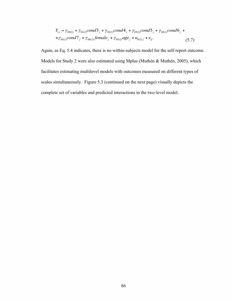
86
(5.7)
Again, as Eq. 5.4 indicates, there is no within-subjects model for the self-report outcome.
Models for Study 2 were also estimated using Mplus (Muthén & Muthén, 2005), which
facilitates estimating multilevel models with outcomes measured on different types of
scales simultaneously. Figure 5.3 (continued on the next page) visually depicts the
complete set of variables and predicted interactions in the two-level model.
1 00(1) 01(1) 02(1) 03(1) 04(1)
05(1) 06(1) 05(1) 0(1)
3 4 5 6
7 .j j j j j
j j j j ij
Y cond cond cond condcond female age u eγ γ γ γ γ
γ γ γ
= + + + + +
+ + + + +

87
Figure 5.3. Two-level model for Study 2

88
CHAPTER 6
RESULTS OF STUDY 2: TRANSIENT AFFECT AND EMOTIONAL CONTAGION
Descriptive Statistics
The descriptive results of the self-report data are presented in Table 6.1 below.
As the Joviality and Sadness scales were transformed into factor scores (see Chapter 3),
the scale means and standard deviations for the two conditions are standardized.
Considering the results on the Joviality scale, we see participants in all three conditions
who watched the happy target video did self-report higher positive affect than those in the
three conditions watching the sad target video. When the outcome was measured by self-
report on the Sadness scale, we see the same overall consistency in the main effect of
stimuli condition; i.e., those in the Sad target conditions report higher sadness than those
in the Happy target conditions.
Table 6.1 Descriptive Statistics for Self-Report by Factor Scores Within Conditions by Joviality and Sadness Scales
Joviality Sadness Condition n M SD M SD
Positive MIP / Happy Target 33 0.562 1.069 -0.090 1.048 Neutral MIP / Happy Target 23 0.256 0.970 -0.337 0.841 Negative MIP / Happy Target 32 0.402 0.824 -0.172 0.674 Positive MIP / Sad Target 32 -0.418 0.968 0.467 1.438 Neutral MIP / Sad Target 30 -0.051 0.942 0.316 0.986 Negative MIP / Sad Target 32 -0.547 0.677 0.349 1.130
The descriptive results of the data from the judges’ ratings are shown in Table 6.2,
which presents the means and standard deviations of the JOV-R and SAD-R ratings on a
seven-point ordinal scale. From the table, we see that the overall scoring of emotion was
relatively low, as all the means are below 1.4 (on a 0 to 6 scale), suggesting that the raters

89
saw very weak expression of emotion in the participants. Similar to the results in Table
4.2, we find that the means on the SAD-R scale are generally higher than on the JOV-R
scale, i.e., the raters were identifying slightly more negative emotion on both conditions.
Table 6.2 Descriptive Statistics for Judges’ Ratings on an Ordinal Scale Within Conditions by JOV-R and SAD-R Items
JOV-R SAD-R Condition n M SD M SD
Intercept 0.610 1.257 0.916 1.217 Positive MIP / Happy Target 33 0.661 1.265 1.158 1.155 Neutral MIP / Happy Target 23 0.662 1.375 1.190 1.317 Negative MIP / Happy Target 32 1.361 1.664 1.051 1.355 Positive MIP / Sad Target 32 0.808 1.419 1.082 1.356 Neutral MIP / Sad Target 30 0.697 1.242 1.334 1.204 Negative MIP / Sad Target 32 0.412 1.008 1.343 1.147
Effectiveness of Mood Induction Procedures
To assess whether the affective imagery tasks produced the intended effect on
participants’ moods, a mixed model analysis of variance was conducted on the three main
mood induction conditions, e.g., the Positive MIP / Happy Target and Positive MIP / Sad
Target conditions were recoded into one new variable, as both conditions experienced the
same Mood Induction Procedure (MIP) prior to viewing the stimuli. Table 6.2 below
summarizes the self-reported intensity of the emotion experienced immediately following
the MIP rated on a 0 to 8 scale, with 8 equivalent to the strongest experience of that
emotion in the participant’s entire life. The average answer to this question in the neutral
condition was around 2.8, a fairly low intensity of emotion. Compared to the neutral
MIP, those engaging in the negative induction procedure reported a 1.239 increase, i.e.,
an average of 4.031, which was significant at p = .002. Those engaging in the positive

90
manipulation also reported a small (0.577) increase in the intensity of the emotion
experienced, but this effect was not significant (p = .144).
Table 6.3 Self-Reported Intensity of the Emotions Experienced During Mood Induction Procedure
Condition Coefficient Standard Error Significance
Positive MIP 0.577 0.393 0.144 Negative MIP 1.239 0.395 0.002 Intercept (Neutral MIP) 2.792 0.292 0.000
The aforementioned results are corroborated in Table 6.3, which presents the self-
reported difficulty of engaging in the MIP. Overall, the participants seemed to have a
hard time engaging in the imagery task, as the reported difficulty on the neutral condition
was 5.180—above average on a 0 to 8 scale. Compared to the neutral condition, those
engaging in the Negative MIP reported the task as being significantly less difficult (β = -
0.730, p = .033). Participants assigned to the positive induction procedure also reported
the task as being less difficult than the neutral condition (though by a smaller magnitude
than those in the Negative MIP conditions), but this effect was not significant (p = .694).
Table 6.4 Self-Reported Difficulty of Engaging in Mood Induction Procedure
Condition Coefficient Standard Error Significance
Positive MIP -0.132 -0.335 0.694 Negative MIP -0.730 -2.153 0.033 Intercept (Neutral MIP) 5.180 0.250 0.000
Two-level Model Results With Positive Affect Outcome Measures
In Table 6.5, the results of the main two-level model are presented when the
outcome was measured on the JOV-R and Joviality scales and the baseline comparison is
to the condition that engaged in the Negative MIP and watched the sad target video

91
(Negative MIP / Sad Target). Considering the Between-Subjects (Level 2) results with
the rating data, we see that participants who were put into a temporary sad mood before
watching the happy stimuli (Negative MIP / Happy Target) were 0.233 of a standard
deviation higher in observed happiness (p = .01) compared to the baseline group
(Negative MIP / Sad Target). No other conditions were significantly different from the
baseline. Considering the demographic factors, we see that age did significantly decrease
the happiness of the participants (β = -0.088, p = .005), controlling for the other
conditions in the model, but gender did not have a significant effect.
Although the judges’ score and self-report measures were positively and
significantly correlated (r = 0.209, p = .005), the magnitude of this correlation was low,
suggesting that the JOV-R and Joviality are still defining separate constructs. We also
note that the Within-Subject factors relating to the assessment of judges’ scores were all
non-significant, suggesting that occasions measured (p = .981), raters (p = .561), and
their interaction (p = .182) were not significantly related to the outcome measured on the
JOV-R scale.
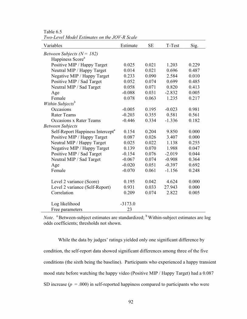
92
Table 6.5 Two-Level Model Estimates on the JOV-R Scale
Variables Estimate SE T-Test Sig.
Between Subjects (N = 182) Happiness Scorea Positive MIP / Happy Target 0.025 0.021 1.203 0.229 Neutral MIP / Happy Target 0.014 0.021 0.696 0.487 Negative MIP / Happy Target 0.233 0.090 2.584 0.010 Positive MIP / Sad Target 0.052 0.074 0.699 0.485 Neutral MIP / Sad Target 0.058 0.071 0.820 0.413 Age -0.088 0.031 -2.832 0.005 Female 0.078 0.063 1.235 0.217 Within Subjectsb Occasions -0.005 0.195 -0.023 0.981 Rater Teams -0.203 0.355 0.581 0.561 Occasions x Rater Teams -0.446 0.334 -1.336 0.182 Between Subjects Self-Report Happiness Intercepta 0.154 0.204 9.850 0.000 Positive MIP / Happy Target 0.087 0.026 3.407 0.000 Neutral MIP / Happy Target 0.025 0.022 1.138 0.255 Negative MIP / Happy Target 0.139 0.070 1.988 0.047 Positive MIP / Sad Target -0.154 0.076 -2.019 0.044 Neutral MIP / Sad Target -0.067 0.074 -0.908 0.364 Age -0.020 0.051 -0.397 0.692 Female -0.070 0.061 -1.156 0.248 Level 2 variance (Score) 0.195 0.042 4.624 0.000 Level 2 variance (Self-Report) 0.931 0.033 27.943 0.000 Correlation 0.209 0.074 2.822 0.005 Log likelihood -3173.0 Free parameters 23
Note. a Between-subject estimates are standardized; b Within-subject estimates are log odds coefficients; thresholds not shown.
While the data by judges’ ratings yielded only one significant difference by
condition, the self-report data showed significant differences among three of the five
conditions (the sixth being the baseline). Participants who experienced a happy transient
mood state before watching the happy video (Positive MIP / Happy Target) had a 0.087
SD increase (p = .000) in self-reported happiness compared to participants who were
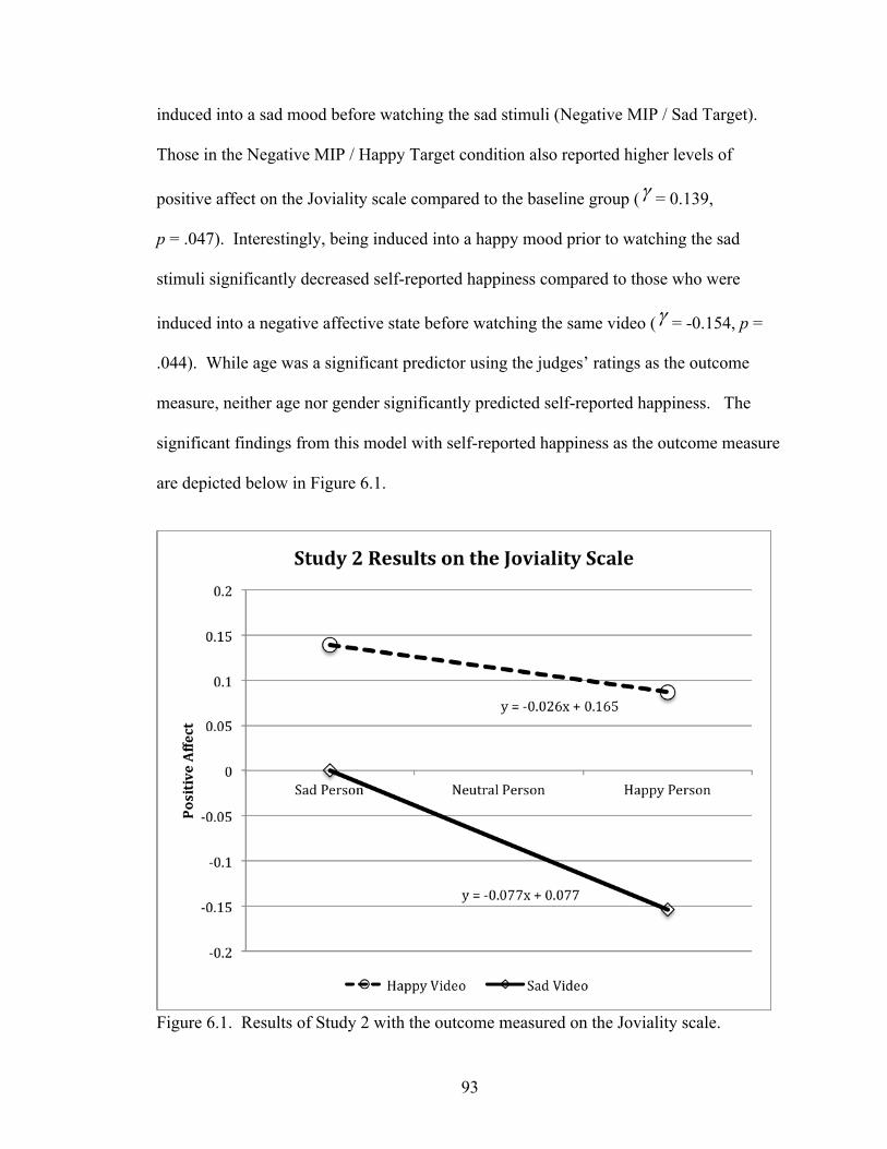
93
induced into a sad mood before watching the sad stimuli (Negative MIP / Sad Target).
Those in the Negative MIP / Happy Target condition also reported higher levels of
positive affect on the Joviality scale compared to the baseline group (γ = 0.139,
p = .047). Interestingly, being induced into a happy mood prior to watching the sad
stimuli significantly decreased self-reported happiness compared to those who were
induced into a negative affective state before watching the same video (γ = -0.154, p =
.044). While age was a significant predictor using the judges’ ratings as the outcome
measure, neither age nor gender significantly predicted self-reported happiness. The
significant findings from this model with self-reported happiness as the outcome measure
are depicted below in Figure 6.1.
Figure 6.1. Results of Study 2 with the outcome measured on the Joviality scale.
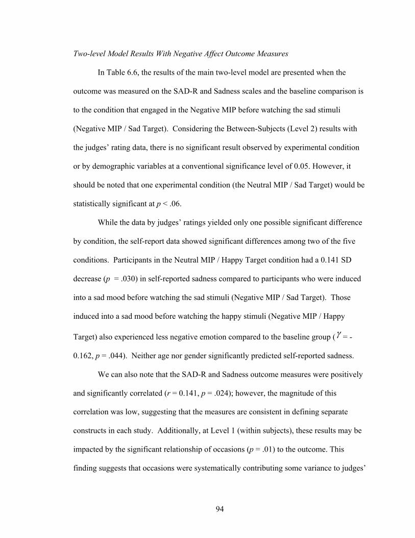
94
Two-level Model Results With Negative Affect Outcome Measures
In Table 6.6, the results of the main two-level model are presented when the
outcome was measured on the SAD-R and Sadness scales and the baseline comparison is
to the condition that engaged in the Negative MIP before watching the sad stimuli
(Negative MIP / Sad Target). Considering the Between-Subjects (Level 2) results with
the judges’ rating data, there is no significant result observed by experimental condition
or by demographic variables at a conventional significance level of 0.05. However, it
should be noted that one experimental condition (the Neutral MIP / Sad Target) would be
statistically significant at p < .06.
While the data by judges’ ratings yielded only one possible significant difference
by condition, the self-report data showed significant differences among two of the five
conditions. Participants in the Neutral MIP / Happy Target condition had a 0.141 SD
decrease (p = .030) in self-reported sadness compared to participants who were induced
into a sad mood before watching the sad stimuli (Negative MIP / Sad Target). Those
induced into a sad mood before watching the happy stimuli (Negative MIP / Happy
Target) also experienced less negative emotion compared to the baseline group (γ = -
0.162, p = .044). Neither age nor gender significantly predicted self-reported sadness.
We can also note that the SAD-R and Sadness outcome measures were positively
and significantly correlated (r = 0.141, p = .024); however, the magnitude of this
correlation was low, suggesting that the measures are consistent in defining separate
constructs in each study. Additionally, at Level 1 (within subjects), these results may be
impacted by the significant relationship of occasions (p = .01) to the outcome. This
finding suggests that occasions were systematically contributing some variance to judges’

95
scores on the SAD-R scale. Raters (p = .091) and their interaction with occasions (p =
.673) were not significantly related to the outcome measured on the SAD-R scale.
Table 6.6 Two-Level Model Estimates on the SAD-R Scale
Variables Estimate SE T-Test Sig. Between Subjects (N = 186) Sadness Scorea Positive MIP / Happy Target 0.148 0.095 1.555 0.120 Neutral MIP / Happy Target 0.076 0.095 0.801 0.423 Negative MIP / Happy Target -0.011 0.111 -0.100 0.921 Positive MIP / Sad Target -0.032 0.114 -0.276 0.782 Neutral MIP / Sad Target 0.179 0.094 1.908 0.056 Age -0.093 0.088 -1.054 0.292 Female 0.048 0.032 1.477 0.140 Within Subjectsb Occasions 0.347 0.134 2.589 0.010 Rater Teams -0.437 0.258 -1.691 0.091 Occasions x Rater Teams -0.096 0.228 -0.422 0.673 Between Subjects Self-Report Sadness Intercepta 0.413 0.244 1.693 0.091 Positive MIP / Happy Target -0.141 0.096 -1.477 0.140 Neutral MIP / Happy Target -0.176 0.081 -2.165 0.030 Negative MIP / Happy Target -0.162 0.080 -2.019 0.044 Positive MIP / Sad Target 0.033 0.109 0.305 0.760 Neutral MIP / Sad Target 0.012 0.089 0.131 0.896 Age -0.043 0.054 -0.795 0.427 Female -0.005 0.036 -0.147 0.883 Level 2 variance (Score) 5.064 0.837 6.051 0.000 Level 2 variance (Self-Report) 1.080 0.226 4.771 0.000 Correlation 0.141 0.062 2.250 0.024 Log likelihood -2667.0 Free parameters 27
Note. a Between-subject estimates are standardized; b Within-subject estimates are log odds coefficients; thresholds not shown.

96
CHAPTER 7
GENERAL DISCUSSION
This investigation began with the premise that emotional contagion is a
phenomenon nearly ubiquitous in daily life—and that while we have scientifically
documented its existence, there remains much to learn about how people catch the
emotions of others and what factors influence this process. One of the factors
hypothesized to influence a person’s susceptibility to emotional contagion is their
affective state, or whether the person is in a happy or sad mood.
Previous research suggested that mood should influence emotional contagion
through attentional or information-processing strategies. In the empirical literature on
emotions, mood has been conceptualized and measured as both an enduring trait, i.e., a
happy or sad personality, and as a transient state affected by temporary manipulation.
However, findings on the impact of trait vs. state emotion have been inconsistent, and the
general relationship between mood and emotional contagion was yet to be explored.
Thus, the purpose of the present investigation was to examine the effect of both enduring
and transient affect on susceptibility to emotional contagion.
Study 1 tested the hypothesis that trait-based affect, i.e., a happy or sad
personality, would affect susceptibility to catching either positive or negative emotions.
Study 2 tested the hypothesis that transient affect, i.e., a momentary happy or sad mood
state, would affect susceptibility to catching either positive or negative emotions.
Previous research suggested two competing processes by which mood—whether
enduring or transient—may impact such emotional contagion. In the addition theory,
people are thought to most likely to catch emotions that are congruent with their current

97
mood. According to the interaction theory, then, the happier people are, the more likely
they should be to catch others’ emotions, regardless of the type of emotion they are
exposed to.
As I evaluate the results of the data analyses in light of these hypotheses and
theoretical predictions, I must begin by considering the validity of the measurement. In
these two studies, outcomes were measured across two dimensions: 1) positive and
negative affect; and 2) self-report and judges’ ratings. Thus, before turning to the
hypotheses, we will examine these two dimensions and consider their impact on the main
findings of this investigation.
Positive vs. Negative Affect
There is strong consensus for the presence of two main structures of self-reported
mood at its broadest level—positive and negative affect (Diener, Larsen, Levine, &
Emmons, 1985; Larsen & Diener, 1985; Russell, 1978, 1979; Watson & Tellegen, 1999).
Given these findings, it seemed theoretically important to measure positive and negative
affect separately on univariate scales, rather than on a bivariate continuous measure, with
happiness on one extreme and sadness on the other (happiness being the absence of
sadness and vice versa). Thus, the outcome measures in this set of studies assessed
positive and negative affect separately, and both types of measurement were included in
the main two-level model. However, preliminary analyses-—including a factor analysis
of the self-report measures, a generalizability study of the raters’ scores, and a review of
the descriptive data—all suggested that positive affect might provide a more reliable and
useful scale of outcome measurement.

98
Factor analysis. In the preliminary analysis of Study 1 (Chapter 3), a factor
analysis was conducted to investigate the reliability of the self-report scales used to
measure the outcomes in both studies, i.e., the Positive Affect (PA), Negative Affect
(NA), Joviality, and Sadness scales from the Positive and Negative Affect Schedule –
Extended Form (PANAS-X). Principal Component Analysis (PCA) yielded a component
matrix for each scale showing which items contributed most strongly to the main
component and its overall reliability (alpha).
When I considered the matrices of the PA, NA, Joviality, and Sadness scales
(Tables 3.4 – 3.7), I found that the positive affect measures (PA and Joviality) had greater
reliability, or alpha levels, than the negative affect scales (NA and Sadness). I noted then
the possibility of using just the highest performing measure, the Joviality scale (α = 0.93),
as the self-report outcome variable in the main two-level model, but I subsequently
decided to keep a measure of negative affect in the analysis for consistency. Therefore,
both the Joviality and Sadness measures were used as self-report outcome variables, in
juxtaposition to the JOV-R and SAD-R scores from the judges’ ratings. However, the
Joviality scale clearly outperformed the Sadness scale (by an alpha difference of .10); an
effect even more pronounced on the general scales, where the reliability of the PA scale
was 0.17 higher than the reliability of the NA scale. Thus, as I interpret the overall
results of the studies, the preliminary factor analysis may justify prioritizing data on the
positive affect dimension.
Generalizability study. In the preliminary analysis of Study 2 (Chapter 5), a
generalizability theory study (G study) was conducted to investigate the reliability of the
rating data by accounting for multiple sources of variance due to raters, occasions, their

99
interaction, and other sources of error. The initial study had five raters evaluate a set of
five participant videos using the five-item Joviality and Sadness scales from the PANAS-
X over three different occasions. Using the magnitudes of potential sources of error from
this G study, a decision study (D study) was conducted to design a measurement
procedure that optimized the use of rater resources. The D study compared the
generalizability coefficient produced by various combinations of raters, items, and
occasions. Ultimately, a combination of two raters, three items on the scale, and two
occasions was selected to most efficiently utilize the number of raters available with
minimal sacrifices to reliability (see Table 5.5). As the five-item Joviality and Sadness
scales were shortened to three-item scales used for the rating task, they were renamed
JOV-R and SAD-R, respectively, to avoid confusion.
In addition to providing information on rater reliability, I noted the total variance
captured on the JOV-R and SAD-R rating scales. When raters assessed the participants
on the JOV-R scale, total variance was 4.659, vs. only 2.262 on the SAD-R scale. In
assessments, it is often beneficial to use a scale that provides more discrimination
between the objects of measurement, and so more variance is useful. More specifically,
variability due to persons (or differences between the participants themselves) is about
60% on the JOV-R scale but only about 41.5% on the SAD-R scale. Thus, the G study
provided justification to emphasize the JOV-R scale as an outcome measure, as it picked
up roughly 45% more variance in participants’ observed emotion compared to the SAD-R
scale. Echoing the conclusion drawn from the factor analysis, the G study suggested that
the main analyses could be conducted using only outcome measures on the positive affect
dimension, i.e., the Joviality and JOV-R scales.

100
Descriptive statistics. Finally, in evaluating the relative merits of the positive and
negative affect outcome measures, we can compare the descriptive results on each type of
scale. In Study 1, considering the self-report descriptive data in Table 4.1, we see the
standardized means and standard deviations for the Joviality and Sadness scales,
previously transformed into factor scores. The Joviality scale picked up considerable
differences between the two experimental conditions in the predicted direction, i.e.,
participants watching the Happy stimuli reported higher happiness than those in the Sad
condition, with a mean difference of 0.738. In comparison, the Sadness scale yielded a
mean difference between conditions of only 0.124, with those watching the Sad stimuli
actually reporting slightly less sadness, in non-conformance to the prediction.
Additionally, on both the self-report (Table 4.1) and raters’ data (Table 4.2), the positive
affect scales (Joviality and JOV-R) provided more variability—i.e., higher standard
deviations—than the negative affect scales (Sadness and SAD-R). Again, scales yielding
higher variability are often desirable in assessment, to allow possible differences between
subjects to be observed. Moreover, the ability of the Joviality scale to pick up a much
larger mean difference between experimental conditions than the Sadness scale also
suggests that it is a better measure for our purposes, consistent with the findings from the
factor analysis in Chapter 3. The descriptive statistics of Study 2 do not suggest a
preference for measurement on either type of affect scale.
Altogether, considering the preliminary factor analysis, G study, and descriptive
data, we have a case to exclude the negative affect outcome measures from our main
analyses, and concentrate on interpreting the data gathered on the Joviality and JOV-R
101
scales. Next, I turn to the question of discriminating between these two types of
outcomes—self-report and judges’ ratings.
Self-Report vs. Judges’ Ratings
After deciding to focus primarily on the positive affect measures, there are two
types of measurement outcomes in the main two-level model: self-report and judges’
ratings. The purpose of our preliminary analyses—factor analysis of the self-report data
and generalizability study of the judges’ ratings—was to improve each type of
measurement before entering it into the model. It is now possible to look at the main
models with positive affect outcomes to compare the qualities of the self-report and
observational measures.
Previous research has found that observational measures (e.g., judges’ ratings)
can be useful when the credibility of self-report is questioned and even when credible
self-report is available, but that behaviors can be difficult for observers to decode
(Hadjistavropoulos & Craig, 2002). Indeed, the results of both studies suggested that
raters had difficulty decoding the emotional displays of the participants. The descriptive
statistics for the observational data (Table 4.2 in Study 1 and Table 6.2 in Study 2)
revealed an overall low scoring of emotion. Across all conditions in both studies, the
average score of emotion on an ordinal scale from 0 to 6 was 0.978—meaning that the
raters evaluated most of the participants as having between “not at all” and “very slight”
visible signs of emotion.
Unfortunately, we cannot compare the mean level of emotion between the
observational data on an ordinal scale and the self-report data, which were transformed
into standardized factor scores. Had the self-report and observational measures been on

102
the same scale, we could compare whether participants were indeed feeling (i.e., self-
reporting) more emotion than the judges perceived. An alternate explanation is that
participants may have actually been experiencing very little emotion, i.e., the judges’
ratings of the participants’ emotion were low because the participants were simply not
feeling strong emotions. However, the explanation that raters had difficulty perceiving
the emotion of the participants is intriguing.
Although we cannot directly compare the means of the self-report and
observational measures, we can investigate their correlation. In Study 1, the Joviality and
JOV-R measures were both weakly and non-significantly correlated (r = .091, p = .295);
in Study 2, the measures were significantly correlated (p = .005), but at a low magnitude
(r = .209). Altogether, these findings provide very little support for the supposition that
self-report and observational measures are identifying the same construct, i.e., raters are
not able to observe participants’ emotion in direct proportion to the strength with which
that emotion is perceived and reported by the participants themselves.
Thus far, the descriptive data suggests that the judges’ were having difficulty
observing emotion in the participants, and the non-correlation of the self-report and rating
scales supports the argument that the two measures were not identifying the same
construct. When we compare the two outcome measures in the main models, we find that
participants did indeed report more emotion than the judges were able to observe. In
Study 1, none of the six between-subject variables was significantly related to judges’
ratings of observed emotion; however, measured by self-report, four of these same six
variables were significant; “Sad Target” and “Subjective Happiness” at α = .05, and
“Emotional Contagion” and “Subjective Happiness*Sad Target” at α = .10. In Study 2,

103
one of the five experimental conditions (the sixth being the baseline) was significant
when measured by judges’ ratings, whereas three of the five conditions were significant
when measured by self-report. Altogether, the main experimental effects in both studies
were stronger when measured by self-report than observation, suggesting that we could
eschew the judges’ ratings and focus on the self-report outcomes. Thus, having
considered both dimensions of outcome measurement—positive vs. negative affect and
self-report vs. observation—and settled on the most appropriate measure, the self-report
of positive affect, i.e., the Joviality scale, we can now turn to our hypotheses and
theoretical predictions.
Testing Hypothesis 1
In review, Hypothesis 1 states: “Trait-based affect, i.e., a happy or sad
personality, affects susceptibility to catching either positive or negative emotions.” Table
4.3 presented the results of the main two-level model with positive affect outcome
measures. Considering the between-subjects results on the Joviality scale, I found that
participants watching the sad target video reported significantly less happiness
( = -0.365, p < .001) compared to their peers watching the happy target video, i.e., the
main effect of emotional contagion by condition was demonstrated.
Next, given that participants in the Sad condition reported their happiness level on
the Joviality scale to be 0.37 of a standard deviation less than those who watched the
Happy target video—i.e., evidence of emotional contagion—we turn to the influence of
enduring affect on this process. Here, we find that the variable measuring trait-based
mood was significantly related to Joviality scores: an increase on the Subjective
Happiness Scale (SHS; the measure of enduring affect) of one standard deviation would
γ

104
result in a 0.67 SD increase in self-reported happiness when assigned to the Happy
condition (p = .004), controlling for the other variables in the model. The significance of
the SHS variable supports the research hypothesis and supports the view that trait-based
affect does indeed affect susceptibility to emotional contagion.
Enduring Affect and Emotional Contagion by Addition or Interaction?
Given that personality-based mood did significantly affect susceptibility to
emotional contagion, I next examine the competing theories on how this process may
operate, i.e., by addition or interaction. According to the addition theory, participants
will be more likely to catch emotions that are congruent with their affective state. For
example, people who tend towards habitual sadness will be more likely to catch sad
emotion from a target. In contrast, the interaction theory predicts that happier people will
be more likely to catch all emotions, in other words, a happy personality increases
susceptibility to emotional contagion.
To test this theory, I return to the significant relationship between SHS and
Joviality). This finding means that as a person becomes habitually happier (i.e., as
indicated through a one standard deviation increase in SHS), he/she picks up more happy
emotion (0.67 SD, to be exact) when watching a happy video. However, both the
addition and interaction theories predict that a happy personality will increase
susceptibility to emotional contagion when watching a happy video. To test between the
theories, we need to look at the interaction term in the model, Subjective Happiness*Sad
Target, which is essentially a test of whether the lines are parallel, as in Figure 3.1, or
non-parallel, as in Figure 3.3.

105
At a lenient test of significance (α = .10), the interaction between condition and
SHS was significant ( = -.379, p = .077). This finding provides cautious support for the
premise that a person with a happy personality (i.e., with a high score on the SHS) will
decrease in happiness by an additional .379 of a standard deviation when watching a sad
video. In essence, the interaction term tests whether the relationship between the target
type (happy or sad) and self-reported emotional response is contingent on reported
subjective happiness. More specifically, the finding suggests that having a self-reported
happy personality becomes an added disadvantage in the Sad Target condition, which
then gets added to the person’s overall score. Thus, if a person’s average reported
happiness is already declining by being in the Sad Target condition (-0.365), an
individual with a reported happy personality (i.e., 1-SD above the mean) will decrease
their happiness even more (-0.369 + -0.379 = -0.748) than someone at an average level of
happiness by-trait. Thus, if we decide to accept the interaction term at a lenient level of
significance, it provides support for interaction theory as the process by which mood
affects emotional contagion; i.e., happy people are more susceptible to catching both
happy and sad emotions, as shown in Figure 3.3
Testing Hypothesis 2
In review, Hypothesis 2 states: “Transient affect, i.e., a happy or sad mood state,
affects susceptibility to catching either positive or negative emotions.” The descriptive
data on the self-report scales in Table 6.1 provides general support for the main effect of
the Happy target condition, as the participants in the three conditions that watched the
Happy Target all had higher means on the Joviality scale than the participants in the
conditions who watched the Sad Target. The same main effect of target condition was
γ

106
also observed on the Sadness scale. Thus, the descriptive data provide preliminary
support that emotional contagion did indeed take place as predicted.
However, to know whether transient mood actually affected susceptibility to
emotional contagion, it is necessary that at least one of the experimental conditions be
statistically significant. In Table 6.5, three of the five conditions (the sixth condition
being the reference group) were significant, which supports the hypothesis that transient
mood impacts emotional contagion. Having any of the mood conditions be significantly
related to the outcome on the Joviality scale implies that transient affect did indeed affect
susceptibility to emotional contagion; in order to investigate the process by which this
contagion occurred, we can examine which specific conditions were significant.
Transient Affect and Emotional Contagion by Addition or Interaction?
With the hypothesis that transient affect affects emotional contagion evidentially
supported, I can now consider the theoretical predictions for how mood may impact
catching another’s emotions. To investigate the theories, we can refer back to Figures 3.1
and 3.3, which show the addition and interaction theories with positive affect as a
dependent variable, respectively.
In the two-level model, all conditions are compared to a baseline control group,
which was selected to be the condition in which participants were induced into a sad
mood prior to watching a sad video (Negative MIP / Sad Target). According to the
addition theory, people should catch emotions congruent with their current mood state,
and as Figure 3.1 suggests, every condition is predicted to have higher levels of positive
affect than the Negative MIP / Sad Target condition.

107
According to the interaction hypothesis, people in a happy mood should be more
susceptible to catching all emotions. Considering the inequality (“<”) shape created by
the prediction lines in Figure 3.3, we see that the baseline group is at the left-most point
of conjunction—and that the Negative MIP / Happy Target group is predicted to be at
roughly the same level of positive affect.
Figure 3.3. Interaction theory: Positive affect as dependent variable
Moving upward along the top line of the inequality sign, which represents those
watching the happy video, we see that the Positive MIP / Happy Target condition is
predicted to be significantly higher than the baseline group, with the Neutral MIP /
Happy Target somewhere in between. Moving downward along the bottom line of the
inequality sign, representing those watching the sad video, we find the Positive MIP / Sad
Target condition significantly lower in positive affect than the baseline group, with the
neutral MIP condition in between.
-‐2.5
-‐2
-‐1.5
-‐1
-‐0.5
0
0.5
1
1.5
2
2.5
Sad Person Neutral Person Happy Person
Positive Affect
Interaction Theory: Positive Affect as Dependent Variable
Happy Video, interaction Sad Video, interaction

108
To simplify the analysis, if the interaction theory holds, we can compare the
positive affect levels of the three main points of the inequality sign and hope to find the
following ascending order, beginning with the lowest group: 1) Positive MIP / Sad
Target; 2) Negative MIP / Sad Target; 3) Positive MIP / Happy Target. In other words,
compared to the Negative MIP / Sad Target condition, the Positive MIP / Happy Target
condition should be higher in positive affect, and the Positive MIP / Sad Target condition
even lower in positive affect.
Consulting Table 6.5, we find that three of the conditions were significantly
related to the baseline condition. Considering our first point of interest, we find that
being induced into a happy mood prior to watching the sad stimuli (Positive MIP / Sad
Target) did significantly decrease self-reported happiness compared to the baseline group
by about 0.15 SD, i.e., the Positive MIP / Sad Target condition was lower in positive
affect compared to the Negative MIP / Sad Target condition. This finding alone is the
key point in support of the interaction theory, as it opposes the addition theory, which
would predict every condition to be higher in positive affect than the baseline group.
Next, we see that participants who experienced a happy transient mood state
before watching the happy video (Positive MIP / Happy Target) had a 0.087 SD increase
in self-reported happiness compared to participants who were induced into a sad mood
before watching the sad stimuli (Negative MIP / Sad Target). This finding completes the
most simple checkpoints of the interaction theory, i.e., that positive affect be lower in the
Positive MIP / Sad Target condition and higher in the Positive MIP / Happy Target
condition than the baseline Negative MIP / Sad Target group.

109
According to the interaction theory, the final significant condition, Negative MIP
/ Happy Target, should be relatively close in affect to the baseline group, i.e., we find the
two conditions at the same conjunction in the inequality-shaped prediction figure. While
we do find that it is relatively close to the baseline, with an increase of only 0.14 SD over
the Negative MIP / Sad Target group, this increase is actually higher than the Positive
MIP / Happy Target group, which does not conform to the prediction. This finding may
be indicative of the strong power of positive emotional contagion, above the affect of
current mood state; i.e., if you are in a sad mood, a positive emotional target can lift you
up even higher than if you started in a happy mood.
Conclusion
In sum, these studies suggest that affect, whether enduring or transient, does
indeed affect susceptibility to emotional contagion. Moreover, this investigation suggests
the relationship between mood and emotional contagion is an interactive one; i.e., that
being in a happy mood makes a person more likely to catch the emotions of others.
A limitation of this study was the inability of the raters to strongly detect the
participants’ emotional displays. The literature on facial expressions and mimicking
suggests that the participants should have expressed more emotion, and the inability of
the raters to identify these displays is inconsistent. Ideally, we would have liked to see a
stronger correlation between the judges’ ratings and self-reports of emotion, which points
to an area of future research. What accounts for the differences in performance between
the self-report and observational measures? An investigation of the lower performance of
the judges’ ratings would improve our understanding of how emotion is experienced,
expressed, and measured.
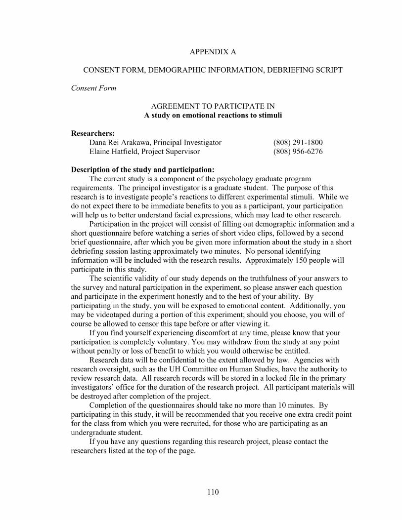
110
APPENDIX A
CONSENT FORM, DEMOGRAPHIC INFORMATION, DEBRIEFING SCRIPT
Consent Form
AGREEMENT TO PARTICIPATE IN A study on emotional reactions to stimuli
Researchers: Dana Rei Arakawa, Principal Investigator (808) 291-1800 Elaine Hatfield, Project Supervisor (808) 956-6276 Description of the study and participation: The current study is a component of the psychology graduate program requirements. The principal investigator is a graduate student. The purpose of this research is to investigate people’s reactions to different experimental stimuli. While we do not expect there to be immediate benefits to you as a participant, your participation will help us to better understand facial expressions, which may lead to other research. Participation in the project will consist of filling out demographic information and a short questionnaire before watching a series of short video clips, followed by a second brief questionnaire, after which you be given more information about the study in a short debriefing session lasting approximately two minutes. No personal identifying information will be included with the research results. Approximately 150 people will participate in this study. The scientific validity of our study depends on the truthfulness of your answers to the survey and natural participation in the experiment, so please answer each question and participate in the experiment honestly and to the best of your ability. By participating in the study, you will be exposed to emotional content. Additionally, you may be videotaped during a portion of this experiment; should you choose, you will of course be allowed to censor this tape before or after viewing it. If you find yourself experiencing discomfort at any time, please know that your participation is completely voluntary. You may withdraw from the study at any point without penalty or loss of benefit to which you would otherwise be entitled. Research data will be confidential to the extent allowed by law. Agencies with research oversight, such as the UH Committee on Human Studies, have the authority to review research data. All research records will be stored in a locked file in the primary investigators’ office for the duration of the research project. All participant materials will be destroyed after completion of the project. Completion of the questionnaires should take no more than 10 minutes. By participating in this study, it will be recommended that you receive one extra credit point for the class from which you were recruited, for those who are participating as an undergraduate student. If you have any questions regarding this research project, please contact the researchers listed at the top of the page.
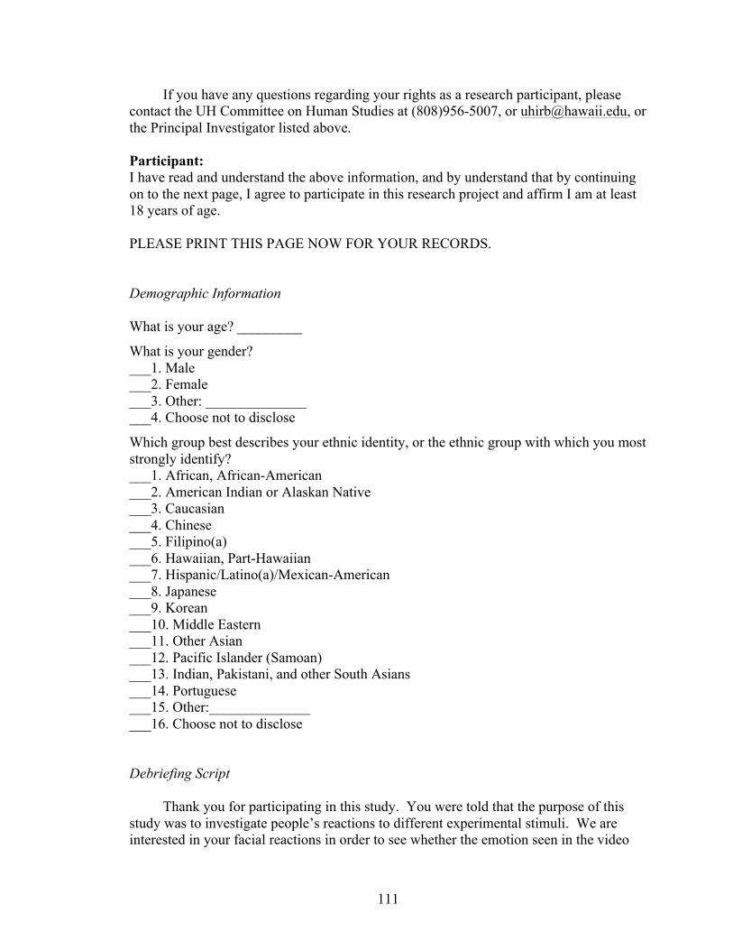
111
If you have any questions regarding your rights as a research participant, please contact the UH Committee on Human Studies at (808)956-5007, or [email protected], or the Principal Investigator listed above. Participant: I have read and understand the above information, and by understand that by continuing on to the next page, I agree to participate in this research project and affirm I am at least 18 years of age. PLEASE PRINT THIS PAGE NOW FOR YOUR RECORDS. Demographic Information What is your age? _________ What is your gender? ___1. Male ___2. Female ___3. Other: ______________ ___4. Choose not to disclose Which group best describes your ethnic identity, or the ethnic group with which you most strongly identify? ___1. African, African-American ___2. American Indian or Alaskan Native ___3. Caucasian ___4. Chinese ___5. Filipino(a) ___6. Hawaiian, Part-Hawaiian ___7. Hispanic/Latino(a)/Mexican-American ___8. Japanese ___9. Korean ___10. Middle Eastern ___11. Other Asian ___12. Pacific Islander (Samoan) ___13. Indian, Pakistani, and other South Asians ___14. Portuguese ___15. Other:______________ ___16. Choose not to disclose
Debriefing Script Thank you for participating in this study. You were told that the purpose of this study was to investigate people’s reactions to different experimental stimuli. We are interested in your facial reactions in order to see whether the emotion seen in the video

112
would be “contagious.” For example, if you smile while seeing people celebrate joyfully, or if you frown while seeing people disappointed. Your reactions to the video clip were recorded by the computer’s camera and will be analyzed by outside raters. Please let us know now or at any time in the future if you would like to see your video recording, which you may also delete at any time.

113
APPENDIX B
SUBJECTIVE HAPPINESS SCALE
For each of the following statements and/or questions, please circle the point on the scale that you feel is most appropriate in describing you. 1. In general I consider myself 1 2 3 4 5 6 7 Not a very happy person
A very happy person
2. Compared to most of my peers, I consider myself 1 2 3 4 5 6 7 Less happy More
happy
3. Some people are generally very happy. They enjoy life regardless of what is going on, getting the most out of everything. To what extent does this characterization describe you? 1 2 3 4 5 6 7 Not at all A great deal 4. Some people are generally not very happy. Although they are not depressed, they never seem as happy as they might be. To what extent does this characterization describe you? 1 2 3 4 5 6 7 Not at all A great deal Scoring: Add together the four item scores. Item 4 is reverse coded, so that if you scored 1 give yourself 7. Then divide the total score by 4 to give a range of 1 to 7. Interpretation: The world adult population scores, on average, between 4.5 and 5.5.

114
APPENDIX C
EMOTIONAL CONTAGION SCALE
This is a scale that measures a variety of feelings and behaviors in various situa-tions. There are no right or wrong answers, so try very hard to be completely honest in your answers. Results are completely confidential. Read each question and indicate the answer which best applies to you. Please answer each question very carefully. Thank you. 1. If someone I’m talking with begins to cry, I get teary-eyed. 4 = Always. Always true for me. 3 = Often. Often true for me. 2 = Rarely. Rarely true for me. 1 = Never. Never true for me. 2. Being with a happy person picks me up when I’m feeling down. 4 = Always. Always true for me. 3 = Often. Often true for me. 2 = Rarely. Rarely true for me. 1 = Never. Never true for me. 3. When someone smiles warmly at me, I smile back and feel warm inside. 4 = Always. Always true for me. 3 = Often. Often true for me. 2 = Rarely. Rarely true for me. 1 = Never. Never true for me. 4. I get filled with sorrow when people talk about the death of their loved ones. 4 = Always. Always true for me. 3 = Often. Often true for me. 2 = Rarely. Rarely true for me. 1 = Never. Never true for me. 5. I clench my jaws and my shoulders get tight when I see the angry faces on the news.
4 = Always. Always true for me. 3 = Often. Often true for me. 2 = Rarely. Rarely true for me. 1 = Never. Never true for me.

115
6. When I look into the eyes of the one I love, my mind is filled with thoughts of romance.
4 = Always. Always true for me. 3 = Often. Often true for me. 2 = Rarely. Rarely true for me. 1 = Never. Never true for me. 7. It irritates me to be around angry people. 4 = Always. Always true for me. 3 = Often. Often true for me. 2 = Rarely. Rarely true for me. 1 = Never. Never true for me. 8. Watching the fearful faces of victims on the news makes me try to imagine how they
might be feeling.
4 = Always. Always true for me. 3 = Often. Often true for me. 2 = Rarely. Rarely true for me. 1 = Never. Never true for me. 9. I melt when the one I love holds me close. 4 = Always. Always true for me. 3 = Often. Often true for me. 2 = Rarely. Rarely true for me. 1 = Never. Never true for me. 10. I tense when overhearing an angry quarrel 4 = Always. Always true for me. 3 = Often. Often true for me. 2 = Rarely. Rarely true for me. 1 = Never. Never true for me. 11. Being around happy people fills my mind with happy thoughts. 4 = Always. Always true for me. 3 = Often. Often true for me. 2 = Rarely. Rarely true for me. 1 = Never. Never true for me. 12. I sense my body responding when the one I love touches me. 4 = Always. Always true for me. 3 = Often. Often true for me. 2 = Rarely. Rarely true for me. 1 = Never. Never true for me.

116
13. I notice myself getting tense when I’m around people who are stressed out. 4 = Always. Always true for me. 3 = Often. Often true for me. 2 = Rarely. Rarely true for me. 1 = Never. Never true for me. 14. I cry at sad movies. 4 = Always. Always true for me. 3 = Often. Often true for me. 2 = Rarely. Rarely true for me. 1 = Never. Never true for me. 15. Listening to the shrill screams of a terrified child in a dentist’s waiting room makes
me feel nervous. 4 = Always. Always true for me. 3 = Often. Often true for me. 2 = Rarely. Rarely true for me. 1 = Never. Never true for me. Scoring: Happiness items – 2, 3, & 11; Love items = 6, 9, & 12; Fear items = 8, 13, & 15; Anger items 5, 7, & 10; Sadness items = 1, 4, &14. Total score = all items. Interpretation: The higher the score, the more susceptible to emotional contagion a person would be said to be.
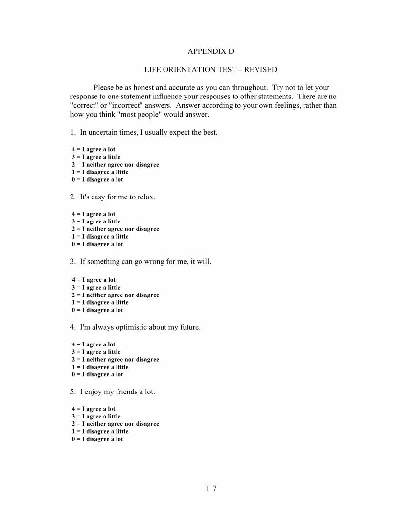
117
APPENDIX D
LIFE ORIENTATION TEST – REVISED
Please be as honest and accurate as you can throughout. Try not to let your response to one statement influence your responses to other statements. There are no "correct" or "incorrect" answers. Answer according to your own feelings, rather than how you think "most people" would answer.
1. In uncertain times, I usually expect the best. 4 = I agree a lot 3 = I agree a little 2 = I neither agree nor disagree 1 = I disagree a little 0 = I disagree a lot 2. It's easy for me to relax. 4 = I agree a lot 3 = I agree a little 2 = I neither agree nor disagree 1 = I disagree a little 0 = I disagree a lot 3. If something can go wrong for me, it will. 4 = I agree a lot 3 = I agree a little 2 = I neither agree nor disagree 1 = I disagree a little 0 = I disagree a lot 4. I'm always optimistic about my future. 4 = I agree a lot 3 = I agree a little 2 = I neither agree nor disagree 1 = I disagree a little 0 = I disagree a lot 5. I enjoy my friends a lot. 4 = I agree a lot 3 = I agree a little 2 = I neither agree nor disagree 1 = I disagree a little 0 = I disagree a lot

118
6. It's important for me to keep busy. 4 = I agree a lot 3 = I agree a little 2 = I neither agree nor disagree 1 = I disagree a little 0 = I disagree a lot 7. I hardly ever expect things to go my way. 4 = I agree a lot 3 = I agree a little 2 = I neither agree nor disagree 1 = I disagree a little 0 = I disagree a lot 8. I don't get upset too easily. 4 = I agree a lot 3 = I agree a little 2 = I neither agree nor disagree 1 = I disagree a little 0 = I disagree a lot 9. I rarely count on good things happening to me. 4 = I agree a lot 3 = I agree a little 2 = I neither agree nor disagree 1 = I disagree a little 0 = I disagree a lot 10. Overall, I expect more good things to happen to me than bad. 4 = I agree a lot 3 = I agree a little 2 = I neither agree nor disagree 1 = I disagree a little 0 = I disagree a lot Scoring: Items 2, 5, 6, and 8 are fillers and therefore should be excluded. Add the scores for the remaining items to calculate the final score. Interpretation: There are no ‘cut-offs’ for optimism or pessimism. Higher scores reflect higher levels of optimism.

119
APPENDIX E
POSITIVE AND NEGATIVE AFFECT SCHEDULE – EXPANDED FORM
This scale consists of a number of words and phrases that describe different feelings and emotions. Read each item and then mark the appropriate answer in the space next to that word. Indicate to what extent you have felt this way right now, at this present moment. Use the following scale to record your answers:
1 2 3 4 5 Very slightly or
not at all A little Moderately Quite a bit Extremely
Positive Affect (PA) Scale
active, alert, attentive, determined, enthusiastic, excited, inspired, interested, proud, strong
Negative Affect (NA) Scale
afraid, scared, nervous, jittery, irritable, hostile, guilty, ashamed, upset, distressed
Joviality Scale13 happy, joyful, delighted, cheerful, excited, enthusiastic, lively, energetic
Sadness Scale sad, blue, downhearted, alone, lonely Scoring: To calculate positive affect (PA), add the scores for the ten items: active, alert, attentive, determined, enthusiastic, excited, inspired, interested, proud, and strong. The total score can vary from 10 to 50.
To calculate negative affect (NA), add the scores for the following ten items: afraid, scared, nervous, jittery, irritable, hostile, guilty, ashamed, upset, and distressed. The total score can vary from 10 to 50.
To calculate the Joviality score, add the scores for the following five items: happy, joyful, cheerful, excited, and enthusiastic. The total score can vary from 5 to 25.
To calculate the Sadness score, add the scores for the following five items: sad, blue, downhearted, alone, and lonely. The total score can vary from 5 to 25. Interpretation: There are no ‘cut-offs’; higher scores reflect higher levels of the construct in question, i.e., positive affect, negative affect, joviality, or sadness. 13 As noted in the discussion of the Joviality Scale in Chapter 3, the three weakest items (delighted, lively, energetic) were excluded to form a five-item measure commensurate with the Sadness Scale.

120
REFERENCES Adamatzky, A. (2005). Dynamics of crowd-minds: Patterns of irrationality in emotions,
beliefs and actions. London: World Scientific Alloy, L.B., & Abramson, L.Y. (1979). Judgment of contingency in depressed and
nondepressed students: Sadder but wiser? Journal of Experimental Psychology, 108(4), 441-485.
Alloy, L.B., Abramson, L.Y., & Viscusi, D. (1981). Induced mood and the illusion of control. Journal of Personality and Social Psychology, 41(6), 1129-1140.
Almagor, M., & Ben-Porath, Y.S. (1989). The two-factor model of self-reported mood: A cross-cultural replication. Journal of personality assessment, 53(1), 10-21.
Ambady, N., & Gray, H.M. (2002). On being sad and mistaken: Mood effects on the accuracy of thin-slice judgments. Journal of Personality and Social Psychology, 83(4), 947.
American Psychiatric Association. (2000). Quick Reference to the Diagnostic Criteria from the DSM-IV-TR. Washington, DC: American Psychiatric Association.
Baker, R.C., & Gutterfreund, D.G. (1993). The effects of written autobiographical recollection induction procedures on mood. Journal of Clinical Psychology, 49, 563-568.
Barsade, S.G. (2002). The ripple effect: Emotional contagion and its influence on group behavior. Administrative Science Quarterly, 644-675.
Baumeister, R.F., Bratslavsky, E., Finkenauer, C., & Vohs, K.D. (2001). Bad is stronger than good. Review of General Psychology, 5(4), 323-370.
Baumeister, R.F., Gailliot, M., DeWall, C.N., & Oaten, M. (2006). Self Regulation and Personality: How Interventions Increase Regulatory Success, and How Depletion Moderates the Effects of Traits on Behavior. Journal of personality, 74(6), 1773-1802.
Beck, A.T., Rush, J., Shaw, B.F., & Emery, G. (1987). Cognitive therapy of depression. New York: The Guilford Press.
Bem, D.J. (1967). Self-perception: An alternative interpretation of cognitive dissonance phenomena. Psychological Review, 74(3), 183-200.
Bernieri, F.J., Davis, J.M., Rosenthal, R., & Knee, C.R. (1994). Interactional synchrony and rapport: Measuring synchrony in displays devoid of sound and facial affect. Personality and Social Psychology Bulletin, 20(3), 303-311.
Bodenhausen, G.V., Sheppard, L.A., & Kramer, G.P. (1994). Negative affect and social judgment: The differential impact of anger and sadness. European Journal of Social Psychology, 24(1), 45-62.
Bouhuys, A.L., Bloem, G.M., & Groothuis, T.G.G. (1995). Induction of depressed and elated mood by music influences the perception of facial emotional expressions in healthy subjects. Journal of Affective Disorders, 33(4), 215-226.
Bourgeois, P., & Hess, U. (2008). The impact of social context on mimicry. Biological psychology, 77(3), 343-352.
Bower, G.H. (1981). Mood and memory. American Psychologist, 36(2), 129-148. Buchwald, A.M., Strack, S., & Coyne, J.C. (1981). Demand characteristics and the
Velten mood induction procedure. Journal of Consulting and Clinical Psychology, 49(3), 478-479.

121
Cacioppo, J.T., Uchino, B.N., Crites, S.L., Snydersmith, M.A., Smith, G., Berntson, G.G., & Lang, P.J. (1992). Relationship between facial expressiveness and sympathetic activation in emotion: A critical review, with emphasis on modeling underlying mechanisms and individual differences. Journal of Personality and Social Psychology, 62(1), 110.
Campbell, J.D., & Fehr, B. (1990). Self-esteem and perceptions of conveyed impressions: Is negative affectivity associated with greater realism? Journal of Personality and Social Psychology, 58(1), 122-133.
Cappella, J.N., & Planalp, S. (1981). Talk and silence sequences in informal conversations III: Interspeaker influence. Human communication research, 7(2), 117-132.
Carlson, J.G., & Hatfield, E. (1992). Psychology of emotion. Fort Worth, TX: Harcourt Brace Jovanovich.
Chapple, E.D. (1982). Movement and sound: The musical language of body rhythms in interaction. In M. Davis (Ed.), Interacton rhythms: Periodicity in communicative behavior (pp. 31-52). New York: Human Sciences Press.
Coan, J.A., & Allen, J.B. (2007). Handbook of emotion elicitation and assessment. New York: Oxford University Press.
Condon, W.S. (1982). Cultural microrhythms Interaction rhythms: Periodicity in communicative behavior (pp. 53-76). New York: Human Sciences Press.
Condon, W.S., & Ogston, W.D. (1966). Sound film analysis of normal and pathological behavior patterns. Journal of Nervous and Mental Disease, 143, 338-347.
Coyne, J.C. (1976). Depression and the response of others. Journal of abnormal psychology, 85(2), 186-193.
Cronbach, L.J., Glesser, G.C., Nanda, H., & Rajaratnam, N. (1972). The dependability of behavioral measurements: Theory of generalizability for scores and profiles. New York, NY: Wiley.
Dahlsgaard, K., Peterson, C., & Seligman, M.E.P. (2005). Shared Virtue: The convergence of valued human strengths across culture and history. Review of General Psychology, 9(3), 203-213.
David, A.S. (1989). Perceptual asymmetry for happy-sad chimeric faces: effects of mood. Neuropsychologia, 27(10), 1289-1300.
Davies, S. (2011). Infectious music: music-listener emotional contagion. In P. Goldie & A. Coplan (Eds.), Empathy: Philosophical and Psychological Perspectives. New York: Oxford University Press.
Davis, M.R. (1985). Perceptual and affective reverberation components. In A. B. Goldstein & G. Y. Michaels (Eds.), Empathy: Development, training, and consequences (pp. 62-108). Hillsdale, NJ: Erlbaum.
Decety, J., & Jackson, P.L. (2004). The functional architecture of human empathy. Behavioral and cognitive neuroscience reviews, 3(2), 71-100.
Delp, M.J., & Sackeim, H.A. (1987). Effects of mood on lacrimal flow: Sex differences and asymmetry. Psychophysiology, 24(5), 550-556.
Diener, E. (1984). Subjective well-being. Psychological Bulletin, 95(3), 542-575. Diener, E. (2000). Subjective well-being: The science of happiness and a proposal for a
national index. American Psychologist, 55(1), 34-43.

122
Diener, E., Emmons, R.A., Larsen, R.J., & Griffin, S. (1985). The satisfaction with life scale. Journal of personality assessment, 49(1), 71-75.
Diener, E., Larsen, R.J., Levine, S., & Emmons, R.A. (1985). Intensity and frequency: Dimensions underlying positive and negative affect. Journal of Personality and Social Psychology, 48(5), 1253-1265.
Diener, E., Lucas, R.E., Oishi, S., & Suh, E.M. (2002). Looking up and looking down: Weighting good and bad information in life satisfaction judgments. Personality and Social Psychology Bulletin, 28(4), 437-445.
Diener, E., & Seligman, M.E.P. (2002). Very happy people. Psychological Science, 13(1), 81.
Doherty, R.W. (1997). The emotional contagion scale: A measure of individual differences. Journal of Nonverbal Behavior, 21(2), 131-154.
Duclos, S.E., & Laird, J.D. (2001). The deliberate control of emotional experience through control of expressions. Cognition & Emotion, 15(1), 27-56.
Duclos, S.E., Laird, J.D., Schneider, E., Sexter, M., Stern, L., & Van Lighten, O. (1989). Emotion-specific effects of facial expressions and postures on emotional experience. Journal of Personality and Social Psychology, 57(1), 100-108.
Dunning, D., & Story, A.L. (1991). Depression, realism, and the overconfidence effect: Are the sadder wiser when predicting future actions and events? Journal of Personality and Social Psychology, 61(4), 521-532.
Eich, E., Kihlstrom, J.F., Bower, G.H., Forgas, J.P., & Niedenthal, P.M. . (2000). Cognition and emotion. New York: Oxford University Press.
Ekman, P. (2007). Emotions revealed: Recognizing faces and feelings to improve communication and emotional life. New York, NY: St. Martin's Griffin.
Ekman, P., & Friesen, W.V. (1978). Facial action coding system: A technique for the measurement of facial movement. Palo Alto, CA: Consulting Psychologists Press.
Ekman, P., Friesen, W.V., O'Sullivan, M., Chan, A., Diacoyanni-Tarlatzis, I., Heider, K., . . . Ricci-Bitti, P.E. (1987). Universals and cultural differences in the judgments of facial expressions of emotion. Journal of Personality and Social Psychology, 53(4), 712-717.
Ellis, H.C., Thomas, R.L., & Rodriguez, I.A. (1984). Emotional mood states and memory: Elaborative encoding, semantics processing, and cognitive effort. Journal of Experimental Psychology: Learning, Memory, and Cognition, 10(3), 470-482.
Evans, R.R., Burnett, D.O., Kendrick, O.W., Macrina, D.M., Snyder, S.W., Roy, J.P.L., & Stephens, B.C. (2009). Developing Valid and Reliable Online Survey Instruments Using Commercial Software Programs. Journal of Consumer Health on the Internet, 13(1), 42-52.
Field, A.P. (2009). Discovering statistics using SPSS (3rd ed.). Thousand Oaks, CA: Sage.
Finegan, J.E., & Seligman, C. (1995). In defense of the Velten mood induction procedure. Canadian Journal of Behavioural Science/Revue canadienne des sciences du comportement, 27(4), 405-419.
Fischer, K.W., Shaver, P.R., & Carnochan, P. (1990). How emotions develop and how they organise development. Cognition and Emotion, 4(2), 81-127.
123
Forgas, J.P. (1992). On mood and peculiar people: Affect and person typicality in impression formation. Journal of Personality and Social Psychology, 62(5), 863.
Forgas, J.P. (1998). On being happy and mistaken: Mood effects on the fundamental attribution error. Journal of Personality and Social Psychology, 75(2), 318-331.
Forgas, J.P., & Bower, G.H. (1987). Mood effects on person-perception judgments. Journal of Personality and Social Psychology, 53(1), 53-60.
Fredrickson, B.L. (2004). The broaden-and-build theory of positive emotions. Philosophical Transactions of the Royal Society B: Biological Sciences, 359(1449), 1367.
Fredrickson, B.L., & Losada, M.F. (2005). Positive affect and the complex dynamics of human flourishing. American Psychologist, 60(7), 678.
Friedman, H.S., Prince, L.M., Riggio, R.E., & DiMatteo, M.R. (1980). Understanding and assessing nonverbal expressiveness: The Affective Communication Test. Journal of Personality and Social Psychology; Journal of Personality and Social Psychology, 39(2), 333-351.
Friedman, H.S., & Riggio, R.E. (1981). Effect of individual differences in nonverbal expressiveness on transmission of emotion. Journal of Nonverbal Behavior, 6(2), 96-104.
Gerrards‐Hesse, A., Spies, K., & Hesse, F.W. (1994). Experimental inductions of emotional states and their effectiveness: A review. British Journal of Psychology, 85(1), 55-78.
Giannini, A.J., Folts, D.J., Melemis, S.M., Giannini, M.C., & Loiselle, R.H. (1995). Depressed men's lower ability to interpret nonverbal cues: A preliminary study. Perceptual and motor skills, 81(2), 555-560.
Goleman, D. (2006). Emotional intelligence. New York: Bantam Dell. Goodwin, A.M., & Williams, J.M.G. (1982). Mood induction research: Its implications
for clinical depression. Behaviour research and therapy, 20(4), 373-382. Gotlib, I.H., Krasnoperova, E., Yue, D.N., & Joormann, J. (2004). Attentional biases for
negative interpersonal stimuli in clinical depression. Journal of abnormal psychology, 113(1), 127-135.
Gotlib, I.H., & Meltzer, S.J. (1987). Depression and the perception of social skill in dyadic interaction. Cognitive Therapy and Research, 11(1), 41-53.
Gottman, J.M., & Krokoff, L.J. (1989). Marital interaction and satisfaction: A longitudinal view. Journal of Consulting and Clinical Psychology, 57(1), 47.
Gottman, J.M., & Levenson, R.W. (2000). The timing of divorce: Predicting when a couple will divorce over a 14 year period. Journal of Marriage and Family, 62(3), 737-745.
Gur, R.C., Erwin, R.J., Gur, R.E., Zwil, A.S., Heimberg, C., & Kraemer, H.C. (1992). Facial emotion discrimination: Behavioral findings in depression. Psychiatry Research, 42(3), 241-251.
Hadjistavropoulos, T., & Craig, KD. (2002). A theoretical framework for understanding self-report and observational measures of pain: A communications model. Behaviour research and therapy, 40(5), 551-570.
Hale, W.W. (1998). Judgment of facial expressions and depression persistence. Psychiatry Research, 80(3), 265-274.

124
Hall, J.A. (1984). Nonverbal sex differences: Communication accuracy and expressive style. Baltimore, MD: Johns Hopkins University Press.
Hatfield, E., Cacioppo, J., & Rapson, R.L. (1994). Emotional contagion. New York: Cambridge University Press.
Hatfield, E., Cacioppo, J.T., & Rapson, R.L. (1993). Emotional contagion. Current Directions in Psychological Science, 2(3), 96-100.
Hatfield, E., & Rapson, R.L. (2004). Emotional contagion: Religious and ethnic hatreds and global terrorism. In L. Z. Tiedens & C. W. Leach (Eds.), The social life of emotions (pp. 129-143). Cambridge: Cambridge University Press.
Haviland, J.J., & Malatesta, C.Z. (1981). The development of sex differences in nonverbal signals: Fallacies, facts, and fantasies. Gender and nonverbal behavior, 183-208.
Heck, R., Johnsrud, L.K. , & Rosser, V.J. (2000). Administrative effectiveness in higher education: Improving assessment procedures. Research in Higher Education, 41(6), 663-684.
Hefferon, K., & Boniwell, I. (2011). Positive Psychology: Theory, Research and Applications. New York, NY: Open University Press.
Heine, S.J., & Norenzayan, A. (2006). Toward a psychological science for a cultural species. Perspectives on Psychological Science, 1(3), 251-269.
Hess, U., & Blairy, S. (2001). Facial mimicry and emotional contagion to dynamic emotional facial expressions and their influence on decoding accuracy. International Journal of Psychophysiology, 40(2), 129-141.
Hewig, J., Hagemann, D., Seifert, J., Gollwitzer, M., Naumann, E., & Bartussek, D. (2005). A revised film set for the induction of basic emotions. Cognition & Emotion, 19(7), 1095-1109.
Hox, J.J. (2010). Multilevel analysis: Techniques and applications. New York, NY: Routledge.
Hurley, S., & Chater, N. (2005a). Perspectives on imitation: From neuroscience to social Science. Volume 1: Mechanisms of imitation and imitation in animals. Cambridge, MA: MIT Press.
Hurley, S., & Chater, N. (2005b). Perspectives on imitation: From neuroscience to social science. Volume 2: Imitation, human development, and culture. Cambridge, MA: MIT Press.
Iacoboni, M. (2005). Understanding others: Imitation, language, empathy. In S. Hurley & N. Chater (Eds.), Perspectives on imitation: From cognitive neuroscience to social science: Vol 1. Mechanisms of imitation and imitation in animals (pp. 77-101). Cambridge, MA: MIT Press.
Isen, A.M. (1987). Positive affect, cognitive processes, and social behavior. In L. Berkowitz (Ed.), Advances in Experimental Social Psychology (Vol. 20, pp. 203-253). San Diego: Academic Press.
Isen, A.M., Clark, M., & Schwartz, M.F. (1976). Duration of the effect of good mood on helping: " Footprints on the sands of time". Journal of Personality and Social Psychology, 34(3), 385-393.
Isen, A.M., & Daubman, K.A. (1984). The influence of affect on categorization. Journal of Personality and Social Psychology, 47(6), 1206-1217.

125
Isen, A.M., Daubman, K.A., & Nowicki, G.P. (1987). Positive affect facilitates creative problem solving. Journal of Personality and Social Psychology, 52(6), 1122-1131.
Klawans, H.L. (1990). Newton's madness: Further tales of clinical neurology. London: Harper & Row.
LaFrance, M., & Banaji, M. (1992). Toward a reconsideration of the gender-emotion relationship. Emotion and social behavior, 14, 178-201.
Laird, J.D. (1974). Self-attribution of emotion: The effects of expressive behavior on the quality of emotional experience. Journal of Personality and Social Psychology, 29(4), 475-486.
Laird, J.D. (1984). The real role of facial response in the experience of emotion: A reply to Tourangeau and Ellsworth, and others. Journal of Personality and Social Psychology, 47, 909-917.
Laird, J.D., Alibozak, T., Davainis, D., Deignan, K., Fontanella, K., Hong, J., . . . Pacheco, C. (1994). Individual differences in the effects of spontaneous mimicry on emotional contagion. Motivation and Emotion, 18(3), 231-247.
Larsen, R.J., & Diener, E. (1985). A multitrait-multimethod examination of affect structure: Hedonic level and emotional intensity. Personality and Individual Differences, 6(5), 631-636.
Larsen, R.J., & Ketelaar, T. (1991). Personality and susceptibility to positive and negative emotional states. Journal of Personality and Social Psychology, 61(1), 132-140.
Larsen, R.J., & Sinnett, L. (1991). Meta-analysis of experimental manipulations: Some factors affecting the Velten mood induction procedure. Personality and Social Psychology Bulletin, 17(3), 323-334.
Le Bon, G. (1896). The crowd. London: Ernest Benn. Levenson, R.W., Carstensen, L.L., Friesen, W.V., & Ekman, P. (1991). Emotion,
physiology, and expression in old age. Psychology and Aging, 6(1), 28-35. Lewinsohn, P.M., Mischel, W., Chaplin, W., & Barton, R. (1980). Social competence and
depression: The role of illusory self-perceptions. Journal of abnormal psychology, 89(2), 203-212.
Lundqvist, L.O. . (1995). Facial EMG reactions to facial expressions: A case of facial emotional contagion? Scandinavian Journal of Psychology, 36(2), 130-141.
Lyubomirsky, S., King, L., & Diener, E. (2005). The benefits of frequent positive affect: does happiness lead to success? Psychological Bulletin, 131(6), 803.
Lyubomirsky, S., & Lepper, H.S. (1999). A measure of subjective happiness: Preliminary reliability and construct validation. Social Indicators Research, 46(2), 137-155.
Marcoulides, G.A. (1996). Estimating variance components in generalizability theory: The covariance structure analysis approach. Structural Equation Modeling: A Multidisciplinary Journal, 3(3), 290-299.
Marcoulides, G.A. (1998). Applied generalizability theory models. In G. A. Marcoulides (Ed.), Modern methods for business research (pp. 1-22). Mahwah, NJ: Lawrence Erlbaum Associates.
Marcoulides, G.A., & Heck, R. (1992). Assessing instructional leadership effectiveness with "G" theory. International Journal of Educational Management, 6(3), 4-13.

126
Markus, H.R., & Kitayama, S. (1991). Culture and the self: Implications for cognition, emotion, and motivation. Psychological Review, 98(2), 224.
Matlin, M.W., & Stang, D.J. (1978). The Pollyanna principle: Selectivity in language, memory, and thought. Cambridge, MA: Schenkman
Matsumoto, D., LeRoux, J., Wilson-Cohn, C., Raroque, J., Kooken, K., Ekman, P., . . . Yee, A. (2000). A new test to measure emotion recognition ability: Matsumoto and Ekman's Japanese and Caucasian Brief Affect Recognition Test (JACBART). Journal of Nonverbal Behavior, 24(3), 179-209.
Matsumoto, D., & Yoo, S.H. (2006). Toward a new generation of cross-cultural research. Perspectives on Psychological Science, 1(3), 234-250.
Mayer, J.D., & Gaschke, Y.N. (1988). The experience and meta-experience of mood. Journal of Personality and Social Psychology, 55(1), 102-111.
Mayer, J.D., Gaschke, Y.N., Braverman, D.L., & Evans, T.W. (1992). Mood-congruent judgment is a general effect. Journal of Personality and Social Psychology, 63(1), 119-132.
Meyer, G.J., & Shack, J.R. (1989). Structural convergence of mood and personality: Evidence for old and new directions. Journal of Personality and Social Psychology, 57(4), 691.
Mischel, W., & Ayduk, O. (2002). Self-regulation in a Cognitive-Affective Personality System: Attentional control in the service of the self. Self and Identity, 1(2), 113-120.
Mullen, B., Futrell, D., Stairs, D., Tice, D.M., Baumeister, R.F., Dawson, K.E., . . . Kennedy, J.G. (1986). Newcasters' facial expressions and voting behavior of viewers: Can a smile elect a president? Journal of Personality and Social Psychology, 51(2), 291-295.
Muthén, B.O., & Muthén, L.K. (2005). Mplus 4.1 [Computer software]. Los Angeles, CA: Muthén & Muthén.
Pacini, R., Muir, F., & Epstein, S. (1998). Depressive realism from the perspective of cognitive-experiential self-theory. Journal of Personality and Social Psychology, 74(4), 1056-1068.
Park, J., & Banaji, M.R. (2000). Mood and heuristics: The influence of happy and sad states on sensitivity and bias in stereotyping. Journal of Personality and Social Psychology, 78(6), 1005-1023.
Persad, S.M., & Polivy, J. (1993). Differences between depressed and nondepressed individuals in the recognition of and response to facial emotional cues. Journal of abnormal psychology, 102(3), 358-368.
Philippot, P. (1993). Inducing and assessing differentiated emotion-feeling states in the laboratory. Cognition & Emotion, 7(2), 171-193.
Pignatiello, M.F., Camp, C.J., & Rasar, L.A. (1986). Musical mood induction: An alternative to the Velten technique. Journal of abnormal psychology, 95(3), 295-297.
Polivy, J., & Doyle, C. (1980). Laboratory induction of mood states through the reading of self-referent mood statements: Affective changes or demand characteristics? Journal of abnormal psychology, 89(2), 286-290.
Pressman, S.D., & Cohen, S. (2005). Does positive affect influence health? Psychological Bulletin, 131(6), 925-971.

127
Russell, J.A. (1978). Evidence of convergent validity on the dimensions of affect. Journal of Personality and Social Psychology, 36(10), 1152-1168.
Russell, J.A. (1979). Affective space is bipolar. Journal of Personality and Social Psychology, 37(3), 345-356.
Salovey, P., & Birnbaum, D. (1989). Influence of mood on health-relevant cognitions. Journal of Personality and Social Psychology, 57(3), 539-551.
Salovey, P., & Mayer, J.D. (1990). Emotional intelligence. Imagination, cognition, and personality, 9(3), 185-211.
Scheier, M.F., Carver, C.S., & Bridges, M.W. (1994). Distinguishing optimism from neuroticism (and trait anxiety, self-mastery, and self-esteem): A reevaluation of the Life Orientation Test. Journal of Personality and Social Psychology, 67(6), 1063.
Schiffenbauer, A. (1974). Effect of observer's emotional state on judgments of the emotional state of others. Journal of Personality and Social Psychology, 30(1), 31-35.
Schwarz, N. (1990). Feelings as information: Informational and motivational functions of affective states. New York, NY: Guilford Press.
Schwarz, N., & Clore, G.L. (1983). Mood, misattribution, and judgments of well-being: Informative and directive functions of affective states. Journal of Personality and Social Psychology, 45(3), 513-523.
Shavelson, R.J., & Webb, N.M. (1991). Generalizability theory: A primer. Newbury Park, CA: Sage.
Shields, S.A. (1987). Women, men, and the dilemma of emotion. In P. Shaver & C. Hendrick (Eds.), Review of personality and social psychology: Vol. 7. Sex and gender (pp. 229-250). Newbury Park: CA: Sage
Shiota, M.N., Keltner, D., & John, O.P. (2006). Positive emotion dispositions differentially associated with Big Five personality and attachment style. The Journal of Positive Psychology, 1(2), 61-71.
Sinclair, R.C., Mark, M.M., Enzle, M.E., Borkovec, T.D., & Cumbleton, A.G. (1994). Toward a multiple-method view of mood induction: The appropriateness of a modified Velten mood induction technique and the problems of procedures with group assignment to conditions. Basic and Applied Social Psychology, 15(4), 389-408.
Singer, J.A., & Salovey, P. (1988). Mood and memory: Evaluating the network theory of affect. Clinical Psychology Review, 8(2), 211-251.
Skowronski, J.J., & Carlston, D.E. (1989). Negativity and extremity biases in impression formation: A review of explanations. Psychological Bulletin, 105(1), 131-142.
Smith, A. (1759/1976). The theory of moral sentiments. Oxford, England: Clarendon Press.
Smith, G.T., Spillane, N.S., & Annus, A.M. (2006). Implications of an emerging integration of universal and culturally specific psychologies. Perspectives on Psychological Science, 1(3), 211-233.
Snyder, C.R. (2002). Hope theory: Rainbows in the mind. Psychological Inquiry, 13(4), 249-275.

128
Snyder, C.R., Lopez, S.J., & Pedrotti, J.T. (2010). Positive psychology: The scientific and practical explorations of human strengths. Thousand Oaks, CA: Sage Publications.
Terwot, M.M., Kremer, H.H., & Stegge, H. (1991). Effects of children's emotional state on their reactions to emotional expressions: A search for congruency effects. Cognition & Emotion, 5(2), 109-121.
Totterdell, P. (2000). Catching moods and hitting runs: Mood linkage and subjective performance in professional sport teams. Journal of applied Psychology, 85(6), 848.
Van den Bos, K. (2003). On the subjective quality of social justice: the role of affect as information in the psychology of justice judgments. Journal of Personality and Social Psychology, 85(3), 482-498.
Västfjäll, D. (2001). Emotion induction through music: A review of the musical mood induction procedure. Musicae Scientiae(Special Issue: Current trends in the study of music and emotion), 173-211.
Velten, E. (1968). A laboratory task for induction of mood states. Behaviour research and therapy, 6(4), 473-482.
Watson, D., & Clark, L.A. (1999). The PANAS-X: Manual for the positive and negative affect schedule-expanded form. Psychology Publications. The University of Iowa.
Watson, D., Clark, L.A., & Tellegen, A. (1988). Development and validation of brief measures of positive and negative affect: the PANAS scales. Journal of Personality and Social Psychology, 54(6), 1063-1070.
Watson, D., & Tellegen, A. (1999). Issues in dimensional structure of affect—Effects of descriptors, measurement error, and response formats: Comment on Russell and Carroll (1999). Psychological Bulletin, 125(5), 601-610.
Westermann, R., Spies, K., Stahl, G., & Hesse, F.W. (1996). Relative effectiveness and validity of mood induction procedures: A meta‐analysis. European Journal of Social Psychology, 26(4), 557-580.
Wild, B., Erb, M., & Bartels, M. (2001). Are emotions contagious? Evoked emotions while viewing emotionally expressive faces: quality, quantity, time course and gender differences. Psychiatry Research, 102(2), 109-124.
Wild, B., Erb, M., Eyb, M., Bartels, M., & Grodd, W. (2003). Why are smiles contagious? An fMRI study of the interaction between perception of facial affect and facial movements. Psychiatry Research: Neuroimaging, 123(1), 17-36.