a discussion of low order numerical integration formulas for...

A Discussion of Low Order Numerical Integration

Formulas for Rigid and Flexible Multibody Dynamics

Dan Negrut∗

Department of Mechanical EngineeringUniversity of Wisconsin

Madison, WI 53706

Laurent O. Jay†

Department of Mathematics14 MacLean HallUniversity of Iowa

Iowa-City, IA 52242

Naresh Khude‡

Department of Mechanical EngineeringUniversity of Wisconsin

Madison, WI 53706

Abstract

The premise of this work is that the presence of high stiffness and/or frictional con-

tact/impact phenomena limits the effective use of high order integration formulas when

numerically investigating the time evolution of real-life mechanical systems. Produc-

ing a numerical solution relies most often on low order integration formulas of which

the paper investigates three alternatives: Newmark, HHT, and order two BDF. Using

these methods, a first set of three algorithms is obtained as the outcome of a direct

index-3 discretization approach that considers the equations of motion of a multibody

system along with the position kinematic constraints. The second batch of three algo-

rithms draws on the HHT and BDF integration formulas and considers, in addition

∗Corresponding author;e-mail:[email protected]†e-mail:[email protected]‡e-mail:[email protected]

1

to the equations of motion, both the position and velocity kinematic constraint equa-

tions. Numerical experiments are carried out to compare the algorithms in terms of

several metrics: (a) order of convergence, (b) energy preservation, (c) velocity kine-

matic constraint drift, and (d) efficiency. The numerical experiments draw on a set of

three mechanical systems: a rigid slider-crank, a slider-crank with a flexible body, and a

seven body mechanism. The algorithms investigated show good performance in relation

to the asymptotic behavior of the integration error and, with one exception, result in

comparable CPU simulation times with a small premium being paid for enforcing the

velocity kinematic constraints.

INTRODUCTION

A multitude of phenomena, processes, and applications are described in terms of mixed sys-tems of differential equations combined with linear and nonlinear algebraic equations, mostoften corresponding to models coming from engineering, physics, and chemistry. Differentialequations relate certain quantities to their derivatives with respect to time and/or space vari-ables. Algebraic equations usually model conservation laws and constraints present in thesystem. When there are derivatives with respect to only one independent variable (usuallytime) the equations are called differential-algebraic equations (DAEs). DAEs are basicallydifferential equations defined on submanifolds of R

n. For the dynamics of multibody sys-tems, the constrained equations of motion can be expressed in the form (see, for instance,[1, 2])

q = vM (q) v = Q (t,q,v, λ, µ,u (t)) − ΦT

q(q, t)λ− ΓT

v(v,q, t)µ

0 = Φ(q, t)0 = Γ(v,q, t) ,

(1)

where q ∈ Rn are generalized coordinates, v ∈ R

n are generalized velocities, λ ∈ Rm

and µ ∈ Rp are Lagrange multipliers, and u : R → R

c represent time dependent exter-nal dynamics; e.g., control variables. The matrix M(q) is the generalized mass matrix,Q(t,q,v, λ, µ,u(t)) represents the vector of generalized applied forces, Φ(q, t) is the set of mholonomic constraints, i.e., position-level kinematic constraints, and Γ(v,q, t) is the set of pnonholonomic constraints, i.e., velocity-level kinematic constraints [3, 4, 1]. Differentiating

2 Dan Negrut, CND-07-1193

the kinematic constraints with respect to time leads to the additional equations

0 = Φq(q, t)v + Φt(q, t)

0 = Φq(q, t)v + (Φq(q, t)v)qv + 2Φqt(q, t)v + Φtt(q, t)

0 = Γv(v,q, t)v + Γq(v,q, t)v + Γt(v,q, t) .

(2)

Equations (1) and (2) form an over-determined system of DAEs, having strictly more equa-tions than variables. The ability to solve such systems is relevant for several classes ofapplications such as multibody dynamics and molecular dynamics.

When finding the solution of Eqs. (1) and (2), most of the numerical solvers currentlyused share some or all of the following drawbacks: numerical drift that occurs when thesolution does not stay on the manifold of constraints at the position and/or velocity levelsand as such might become nonphysical; inability to deal efficiently with stiffness; loss ofunderlying properties of the exact flow and trajectories; no preservation of invariants suchas energy; introduction of undesired numerical damping; and the reduction of convergenceorder when solving stiff problems that arise often in applications. Whereas techniques forthe numerical solution of ordinary differential equations (ODEs) go back more than threecenturies and are well established, the numerical solution of DAEs has a comparativelyshort history [5, 6, 7]. The first class of numerical techniques eventually applied to DAEswas published in [8] for the solution of ODEs. Since then DAEs have widely penetrated thenumerical analysis, engineering, and scientific computing communities and are increasinglyencountered in practical applications. Still, numerically solving DAEs poses fundamentaldifficulties not encountered when solving ODEs. Specialized numerical techniques have beendeveloped, typically belonging to one of two classes: state-space methods or direct methods.For a recent review of this topic the reader is referred to [9].

State-space methods first reduce the DAEs to a smaller dimension ODE problem, thusbenefiting from the extensive body of knowledge associated with ODE solvers. Specifically,the DAEs induce differential equations on the constraint manifold [10], which can be re-duced on a subspace of the n-dimensional Euclidean space. The resulting state-space ODEs(SSODEs) are integrated using classical numerical integration formulas. The one-to-one lo-cal mapping from the manifold to the subspace of independent coordinates is then used todetermine the point on the manifold corresponding to the solution of the SSODEs. Thisframework formalizes the theory of numerical solution of DAEs using the language of differ-ential manifolds [11]. Practical algorithms drawing on this class of methods are presented in[12, 13, 10, 14]. The main factor that differentiates these algorithms is the choice of manifoldparameterization.

State-space methods have been subject to criticism in two aspects. First, the choice ofparameterization generally is not global. Second, poor choices of the projection space resultin SSODEs that are numerically demanding, mainly at the expense of overall efficiency androbustness of the algorithm [15]. Although the theoretical framework for these methods wasoutlined several years ago [16, 10], it was only relatively recently that implicit numericalintegration methods for DAEs have been proposed in the context of SSODEs for multibodydynamics analysis [17, 18]. The major intrinsic drawback associated with state-space meth-


ods remains the expensive DAE to ODE reduction process that is further exacerbated in thecontext of implicit integration, which is the norm in industry applications.

Alternatively, direct methods discretize the constrained equations of motion in Eq. (1),possibly after reducing the index of the DAEs by considering some or all of the kine-matic constraint equations in Eq. (2). Original contributions in this direction are foundin [19, 20, 5, 21, 22, 23, 24, 25, 26]. When dealing with systems that include flexible sub-structures and bodies, numerical methods have been sought that are capable of introducingcontrollable numerical dissipation to damp out spurious high frequencies, an artifact of thespatial discretization, without affecting the low frequency modes of the system and the ac-curacy of the method [27, 28]. Several methods have been proposed for structural dynamicssimulation, such as the HHT method (also called α-method) [29] and the generalized α-method [30]. These are order two methods proposed in conjunction with ODE problems.For DAEs stemming from multibody dynamics analysis, several α-type algorithms have beenreported in the literature [31, 32]. A thorough discussion of theoretical and implementationaspects related to an HHT-based numerical integrator for the simulation of large mechanicalsystems with flexible bodies and penalty-based contact/impact can be found in [33], whilea convergence analysis of the generalized-α method has been provided in [34]. However,until recently there has been no HHT type method that also stabilized the solution on thevelocity constraint manifold, an attribute that is important in mechatronics applications andin dealing with joint friction/contact models. Two of the six algorithms considered in thisstudy address this issue of velocity constraint stabilization and they draw on work presentedin [35, 36].

The paper is organized as follows: first, the six algorithms investigated in this study areintroduced. For each algorithm, a short overview of existing convergence results is providedalong with the expression of the Jacobian associated with the nonlinear discretization system.The emphasis is on HHT-SI2, a new variable-damping stabilized overdetermined index 2algorithm whose convergence analysis is upcoming [37]. Next, a set of numerical experimentsdrawing on three mechanical systems compares the algorithms in terms of several metrics:global integration error, energy preservation, velocity constraint violation, and efficiency. Aset of brief remarks conclude the paper.

LOW ORDER INTEGRATION ALGORITHMS

The first integration method considered in this study is essentially the BDF method of ordertwo proposed in [8], and it serves the purpose of providing a reference when comparing theperformance of the other algorithms. The second order BDF formula is cast into a formsuitable for direct numerical integration of second order differential equations:

qn+1 = 43qn − 1

3qn−1 + h

(

89qn − 2

9qn−1

)

+ 49h2qn+1

qn+1 = 43qn − 1

3qn−1 + 2

3hqn+1.

(3)


These formulas, used in conjunction with the equations of motion and position kinematicconstraint equations, lead to a second order method herein called NSTIFF:

M(qn+1) qn+1 + (ΦTqλ)n+1 − Qn+1 = 0

94h2 Φ(qn+1, tn+1) = 0.

(4)

As suggested in [33] and recently analyzed in [38], the scaling of the kinematic constraintequations by the inverse of the integration step-size h2 is done in order to prevent an ill-conditioning of the Jacobian JNSTIFF associated with the Newton-type method employedto solve Eq. (4), which is regarded as a nonlinear system in qn+1 and λn+1:

JNSTIFF =

[

M + P ΦTq

Φq 0

]

,

where P = 49h2(M(q) q+(ΦT

qλ)−Q)q−

23hQq. Note that when h→ 0 the condition number

of JNSTIFF remains bounded. The scaling of the position constraint equation by 94h2 leads

to a bounded value. To see this, first note that for all the numerical integration formulasconsidered herein, locally, ||qn+1− qn+1|| = O(h2), where qn+1 is the exact solution and qn+1

is an approximation obtained after taking an integration step. Then,

Φ(q, t) = Φ(q, t) + Φq(q, t) (q − q) + . . .

= Φq(q, t)(q − q) + . . .

where the subscript n + 1 on q, q, and t was dropped for convenience. It follows that9

4h2 Φ(qn+1, tn+1) is O(h0), which justifies the scaling proposed in Eq. (4).

The second numerical integration method considered uses the Newmark formulas [39].It requires the selection of two parameters γ ≥ 1/2, and β ≥ (γ + 1/2)2/4 based on which,given the acceleration qn+1 at the new time step tn+1, the new position and velocity areobtained as

qn+1 = qn + hqn + h2

2[(1 − 2β)qn + 2βqn+1]

qn+1 = qn + h [(1 − γ)qn + γqn+1] .(5)

Given an integration step-size h, the discretization scheme operates on the equations ofmotion and position kinematic constraint equations to lead to the nonlinear system:

(Mq)n+1 + (ΦTqλ)n+1 = Qn+1 (6)

1

βh2Φ(qn+1, tn+1) = 0 . (7)

The method, called hereafter NEWMARK, is order one unless γ = 1/2 and β = 1/4. Thischoice leads to the trapezoidal method, which is known in the literature to have stabil-ity problems when used in conjunction with index-3 DAEs [31]. Note that the JacobianJNEWMARK is identical to JNSTIFF , except that the matrix P is replaced by a matrix Pobtained by replacing 4

9with β and 2

3with γ.

Referred to as HHT-I3, the third method considered in this study relies on the HHTmethod [29], widely used in the structural dynamics community and first considered in the


context of multibody dynamics analysis in [31]. HHT-I3 is defined as follows (note that thediscretized equations of motion have been scaled by 1

1+α):


2[(1 − 2β)an + 2βan+1]

qn+1 = qn + h [(1 − γ)an + γan+1]

11+α

(M(q) a)n+1 + (ΦTqλ− Q)n+1 −

α1+α

(ΦTqλ− Q)n = 0

1βh2 Φ(qn+1, tn+1) = 0 .

(8)

The notation used in Eq. (8) is meant to emphasize that there is a distinction between qn+1

and an+1 (compare with Eq. (5)). Concretely, an+1 is an approximation of q(tn + (1 +α)h).This raises some difficulties in choosing a0, an attribute that is associated with the use ofHHT in general and is not specific to HHT-I3. In [36] it is recommended to take a0 = q0

and in spite of this approximation the same convergence results hold for the global behaviorof the method. For more accurate results, an implicit and therefore slightly more involvedway of computing a0 is suggested in [35]. Finally, note that the the last two equations in(8) lead to a nonlinear system that is solved with a Newton-like method for an+1 and λn+1.The associated Jacobian

JHHTI3 =

[

11+α

M + P ΦTq

Φq 0

]

,

does not become ill conditioned when h → 0. Taking the limit, P → 0, and JHHTI3 isnonsingular as long as the kinematic constraints are independent and the symmetric massmatrix is nonsingular.

The last three numerical integration methods considered herein take into account thevelocity kinematic constraint equations. The salient attribute of these methods is a resultingset of consistent generalized velocities, an aspect relevant in frictional contact and controlsapplications. The method referred to as NSTIFF-SI2 is an implementation of the stabilizedindex 2 formulation reported in [20] that uses second order BDF formulas [8]:

qn+1 = 43qn − 1

3qn−1 + 2

3hqn+1

vn+1 = 43vn − 1

3vn−1 + 2

3hvn+1 .

(9)

NSTIFF-SI2 explicitly accounts for the velocity kinematic constraint equations and relieson an extra set of Lagrange multipliers µ to enforce these constraints. The unknowns arev, q, λ, and µ and the new configuration at tn+1 is the solution of the following system ofnonlinear equations:

M(qn+1)vn+1 + ΦTq(qn+1)λn+1 − Q(tn+1,qn+1,vn+1) = 0

vn+1 − qn+1 + ΦTq(qn+1)µn+1

= 032h

Φ(qn+1, tn+1) = 032h

Φq(qn+1, tn+1)vn+1 + 32h

Φt(qn+1, tn+1) = 0 .

(10)


When using a Newton-type method, the associated Jacobian assumes the form

JNSTIFF−SI2 =

M 2h3

(Mv + ΦTqλ− Q)q ΦT

q0

2h3I −I − 2h

3(ΦT

qµ)q 0 ΦT

q

Φq 0 0 0(Φqv)q + Φqt Φq 0 0

Under mild conditions (symmetric nonsingular mass matrix and independent set of kinematicconstraints) it can be easily shown that JNSTIFF SI2 remains nonsingular when h→ 0. Alsonote that in the absence of discretization errors, µ would be identically zero.

The fifth method considered in this study introduces a correction into the Newmark for-mulas based on the constraint accelerations and was shown to have global convergence ordertwo [35, 36]. Given a configuration (qn, qn, an), and defining f(t,q, q) := M−1(q)Q(t,q, q)and r(q, λ) := −M−1 (q)ΦT

qλ, the unknowns qn+1, qn+1, an+1, ψI , and ψII are found as the

solution of the following nonlinear system:


2((1 − 2β)an + 2βan+1)

+ h2

2((1 − b)RI + bRII)

qn+1 = qn + h((1 − γ)qn + γqn+1) + h2(RI + RII)

0 = Φ(qn+1, tn+1)0 = Φq(qn+1, tn+1)qn+1 + Φt(qn+1, tn+1)

an+1 = (1 + α)f(tn+1,qn+1, qn+1) − αf(tn,qn, qn) ,

(11)

where b 6= 1/2 is a free coefficient, RI := r(tn,qn, ψI) , RII := r(tn+1,qn+1, ψII). Thismethod is referred as HHT-ADD and is discussed at length in [35, 36] where local andglobal error analysis results are provided along with an investigation of stability properties.In addition to displaying attractive numerical damping controlled through the parameterα ∈ [−0.3, 0], the method is shown to be order two. The major drawback of this methodis the multiplication by the inverse of the mass matrix. Specifically, this becomes a majorconcern in the inexact-Newton step when dealing with flexible body problems where, due tothe coupling in the deformation modes, the mass matrix can have large dense blocks. TheJacobian JHHT ADD is not provided herein, the interested reader is referred to [36].

The last integration method investigated, HHT-SI2, represents a new algorithm that isanalyzed theoretically in [37]. It represents a variation on the HHT-ADD algorithm thatavoids multiplication by the inverse of the mass matrix. As such, it is amenable to handlingmechanical systems with flexible bodies in which the formulation relies on the floating frameof reference approach [2]. For HHT-SI2 the Newmark integration formulas are modifiedslightly by introducing a correction h2

2a:

qn+1 = qn + hqn +h2

2[(1 − 2β)an + 2βan+1] +

h2

2a (12a)

qn+1 = qn + h [(1 − γ)an + γan+1] . (12b)

In advancing the integration from a given configuration at time tn to tn+1, the unknownsan+1, a, λn+1, and µ are found as the solution of the nonlinear system of equations:


11+α

Mn+1an+1 −(

ΦTqλ− Q

)

n+1+ α

1+α

(

ΦTqλ− Q

)

n= 0

Mn+1a − ΦTq(tn+1,qn+1)µ = 0

1h2 Φ(qn+1, tn+1) = 0

1hΦq(qn+1, tn+1)qn+1 + 1

hΦt(qn+1, tn+1) = 0 ,

(13)

where Mn+1 := M (tn + h(1 + α),qn + h(1 + α)qn). Here a and µ are auxiliary variableslocal to the current time step. Introducing the notation R = h2(ΦT

qµ)q , Q = −βh2(ΦT

qλ−

Q)q + γhQq , F = −β h2

2(ΦT

qλ − Q)q , and V = h(Φq(q, t)q + Φt(q, t))q, the Jacobian

associated with the discretized problem assumes the expression

JHHT−SI2 =

11+α

Mn+1 + Q 12F −ΦT

q0

βR Mn+1 −12R 0 −ΦT

q

βΦq

12Φq 0 0

γΦq + βV 12V 0 0

.

If J0HHT−SI2 = limh→0 JHHT−SI2, then

J0HHT−SI2 =

11+α

Mn+1 0 −ΦTq

0

0 Mn+1 0 −ΦTq

βΦq

12Φq 0 0

γΦq 0 0 0

,

and under mild assumptions (symmetric nonsingular mass matrix and independent set ofkinematic constraints) the matrix J0

HHT−SI2 turns out to be nonsingular. This guaranteesacceptable behavior at small values of the step-size, a situation typically encountered inpenalty-based frictional contact problems. The main result regarding the convergence of thenew method HHT-SI2 is stated as follows. Suppose that the initial configuration at time t0is such that

0 = M(t0,q0)a0 + ΦTqλ0 − Q(t0,q0, q0, λ0)

0 = Φ(t0,q0)

0 = Φt(t0,q0) + Φq(t0,q0)q0

0 = Φtt(t0,q0) + 2Φtq(t0,q0)q0

+ [Φq(t0,q0)q0]q q0 + Φq(t0,q0)a0 ,

and aα −a(t0 +αh) = O(h). Then the numerical approximation (qn, qn, an+α, λn) producedby the HHT-SI2 method in Eqs. (12) and (13) satisfies

qn − q(tn) = O(h2)

qn − q(tn) = O(h2)

an+α − a(tn + αh) = O(h2)

λn − λ(tn) = O(h2) ,

for 0 < h ≤ hmax and tn − t0 = nh ≤ Const, where hmax is suitably chosen. Here q(tn),q(tn), a(tn + αh), and λ(tn) denote the exact value of the respective unknown quantities atthe times indicated in parentheses. A formal proof of this is provided in [37].


Implementation Details

The computational flow associated with any of the six integration methods discussed can beabstracted in the following way. A set of unknowns wn+1 is computed as the solution of anonlinear system Υ(wn+1) = 0. In turn, the position and velocity at the new configurationtn+1 is evaluated based on a set of integration formulas: qn+1 = I1(wn+1), and qn+1 =I2(wn+1). Illustrating this abstraction for HHT-SI2, the expression of Υ is obtained fromEq. (13), I1 is provided by Eq. (12b), and I2 is provided by Eq. (12a). Regardless of themethod used, advancing the solution from tn to tn+1 follows a simple recipe:

tn+1 = tn + h %L1

w(0)n+1 = wn %L2

Do %L3

q(k)n+1 = I1(w

(k)n+1) %L4

q(k)n+1 = I2(w

(k)n+1) %L5

Evaluate Jacobian J %L6

Solve linear system J ∆w(k) = Υ(w(k)n+1) %L7

If ||∆w(k)|| ≤ ǫ then break %L8

Apply correction: w(k+1)n+1 = w

(k)n+1 − ∆w(k) %L9

Enddo %L10

wn+1 = w(k)n+1 %L11

Certain variations of this algorithm can improve its efficiency. For instance, rather thanevaluating it at each time step, the Jacobian can be evaluated less frequently. While acostly proposition in itself, each Jacobian evaluation is necessarily followed by a factorizationstep, which is also costly. Note that although the convergence test relies exclusively on thecorrection norm at line L8 of the pseudocode, the test could also include the norm of residual,i.e. the right side of the linear system in L7.

NUMERICAL EXPERIMENTS

The numerical algorithms NSTIFF, NEWMARK, HHT-I3, NSTIFF-SI2, HHT-ADD, andHHT-SI2 were implemented in MATLAB and used in conjunction with three models. Severalexperiments were run to evaluate the algorithms’ performance and compare them in relationto the order of global convergence, energy preservation, constraint satisfaction, and efficiency.The models considered for testing and comparison of algorithm performance were a slidercrank, a slider crank with a flexible connecting rod, and a seven body mechanism (see, forinstance, [40, 41, 42]). The model parameters and the initial conditions used are summarizedbelow.

a. Slider Crank


y

x

y1’x1’

m1g

L1

θ2

L2

y2’

x2’m2g

c

k

θ1

A

B

O

Figure 1: Slider Crank Figure 2: Seven Body Mechanism

The schematic of a slider crank model including a spring-damper element is shown inFig. (1). The parameters associated with the model are m1 = 3 kg, L1 = 0.3 m, m2

= 0.9 kg, L2 = 0.6 m, k = 100 N/m and c = 5 Ns/m. Both links are symmetric andhomogeneous, and the center of mass is at the midpoint. The initial conditions usedfor simulation of motion were θ1 (0) = 3π/2, θ1(0) = 0 rad/s.

b. Flexible Slider Crank

This model is similar to the rigid slider-crank shown in Fig. (1), except that the springand damper are not included and the connecting rod AB is flexible. The parametervalues used in this model are m1 = 3 kg, L1 = 0.3 m, m2 = 0.9 kg and L2 = 0.6 m,cross-section area S = 5.74E-6 m2, moment of inertia I = 2.765E-8 m4 and Young’smodulus E = 200 GPa. Both links are symmetric and homogeneous, and the center ofmass is at the midpoint. The initial conditions are θ1 (0) = 3π/2, θ1(0) = 1 rad/s. Theequations of motion are formulated using the floating frame of reference formulation,see [2], pp. 231.

c. Seven Body Mechanism

The model is presented in Fig. (2). For this set of numerical experiments, the value ofthe damping c was set zero. An account of the geometry of the mechanism, along withinertia properties and initial conditions is provided in [40]. The mechanism moves dueto a torque applied to crank 1. All bodies in the model are rigid.

Global Convergence Analysis

The goal of the first set of numerical experiments is to assess how the global integration errordecreases with the integration step-size, i.e. to carry out a convergence analysis. From an


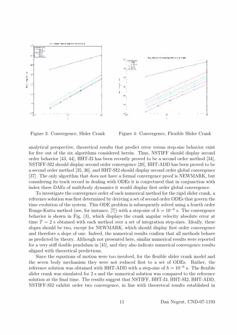
Figure 3: Convergence, Slider Crank Figure 4: Convergence, Flexible Slider Crank

analytical perspective, theoretical results that predict error versus step-size behavior existfor five out of the six algorithms considered herein. Thus, NSTIFF should display secondorder behavior [43, 44], HHT-I3 has been recently proved to be a second order method [34],NSTIFF-SI2 should display second order convergence [20], HHT-ADD has been proved to bea second order method [35, 36], and HHT-SI2 should display second order global convergence[37]. The only algorithm that does not have a formal convergence proof is NEWMARK, butconsidering its track record in dealing with ODEs it is conjectured that in conjunction withindex three DAEs of multibody dynamics it would display first order global convergence.

To investigate the convergence order of each numerical method for the rigid slider crank, areference solution was first determined by deriving a set of second order ODEs that govern thetime evolution of the system. This ODE problem is subsequently solved using a fourth orderRunge-Kutta method (see, for instance, [7]) with a step-size of h = 10−6 s. The convergencebehavior is shown in Fig. (3), which displays the crank angular velocity absolute error attime T = 2 s obtained with each method over a set of integration step-sizes. Ideally, theseslopes should be two, except for NEWMARK, which should display first order convergenceand therefore a slope of one. Indeed, the numerical results confirm that all methods behaveas predicted by theory. Although not presented here, similar numerical results were reportedfor a very stiff double pendulum in [45], and they also indicate numerical convergence resultsaligned with theoretical predictions.

Since the equations of motion were too involved, for the flexible slider crank model andthe seven body mechanism they were not reduced first to a set of ODEs. Rather, thereference solution was obtained with HHT-ADD with a step-size of h = 10−6 s. The flexibleslider crank was simulated for 2 s and the numerical solution was compared to the referencesolution at the final time. The results suggest that NSTIFF, HHT-I3, HHT-SI2, HHT-ADD,NSTIFF-SI2 exhibit order two convergence, in line with theoretical results established in


Figure 5: Convergence, Orientation Figure 6: Convergence, Angular Velocity

conjunction with these algorithms. Furthermore, NEWMARK shows global convergence oforder one for all models. The convergence orders hold both for the generalized coordinatesand their time derivative, that is, both for positions and velocities. Figure (4) displays theconvergence and order for the flexible slider crank; the results reported concern the angularvelocity of the crank. Finally, for body 5 of the seven body mechanism, see Fig. (2), theconvergence plots for its orientation and angular velocity are displayed in Figs. (5) and (6).

Energy preservation

The HHT method came as an improvement over Newmark formulas because it preservedthe A-stability and its attractive numerical damping properties while achieving second-orderaccuracy. In this method, high-frequency oscillations that are not of interest, as well asparasitic high-frequency oscillations that are a byproduct of the finite element discretization,are damped out through the parameter α. The choice of α is based on the desired level ofdamping: the more negative the value of α, the more damping is induced in the numericalsolution. Note that the choice α = 0 leads to the trapezoidal method with no numericaldamping. The effect of this damping can be seen from energy preservation plots shown inFigs. 7 and 8. These energy plots are for the slider-crank model from which the translationaldamper was removed. The system is conservative and, for the particular reference systememployed, the total energy should be constant and equal to zero.

For α = −0.3, the numerical damping-induced dissipation is one order of magnitudemore pronounced than the α = −0.05 case, qualitatively in line with expectations. Evenmore relevant is an investigation of how the numerical energy dissipation changes with thestep-size. Results in Fig. (8) indicate a highly oscillatory pattern. To capture the degree towhich a numerical scheme dissipates energy, an average energy dissipation over an interval


Figure 7: Energy Dissipation at α = - 0.3 Figure 8: Energy Dissipation at α = - 0.05

[0, T ] is computed as

ε(T ) =1

T

∫ T

0

|Etot(t)| dt . (14)

If no numerical dissipation was present in the system then ε(T ) = 0, ∀T > 0. On alog-log scale, Fig. 9 shows this quantity for the rigid slider crank model with no physicaldamping, while Fig. 10 displays the same quantity for the flexible slider crank. This averageenergy error for NEWMARK converges to zero like O(h), while for all the other methodsit converges to zero like O(h2). In other words, the convergence is order O(hq), where qis the order of the method. Although this does not serve as a formal proof, this attributedeserves further investigation, since ε(T ) is an average quantity that captures the energydrift over the entire simulation. Such a result could be relevant, for instance, in the contextof Molecular Dynamics (MD) simulation, where entire classes of integrators are disqualifiedif they do not preserve energy. However, with values in the femtosecond range, the step-sizefor MD simulations might be so small that particularly HHT, through its variable dampingattribute, might in fact be a viable numerical integration formula. This aspect is furtherinvestigated in [46].

Kinematic constraint drift

The rationale behind stabilizing the numerical solution of the index 3 DAE of multibodydynamics using the velocity kinematic constraint equations is to prevent drift in satisfyingthis set of algebraic constraints. Three of the six methods analyzed in this study, namelyHHT-ADD, HHT-SI2, and NSTIFF-SI2, enforce these equations. As such, no velocity con-straint drift is expected in the numerical solution. This is confirmed by the plots in Figs. (11)and (12), which display the velocity constraint violation in the X direction against the ve-locity constraint violation in the Y direction for the rigid slider-crank mechanism for the


Figure 9: Dissipation - Slider Crank Figure 10: Dissipation - Flexible Slider Crank

pin joint between the crank and ground. Data was plotted at each time step and, as antici-pated, confirms that the velocity kinematic constraint equations are satisfied within machineprecision. A qualitatively identical plot for NSTIFF-SI2 is provided in [47].

For NEWMARK, NSTIFF, and HHT-I3, Figs. (13) through (15) report the same infor-mation for the rigid slider crank with no damping obtained during a 10 second simulationwith a step-size h = 2−10s. One remarkable property is that NEWMARK, HHT-I3, andNSTIFF display the same error behavior. Moreover, as the step-size decreases, the box thatbounds the plot shrinks but the shape of the curves remains the same for all three inte-gration methods. The cause of this behavior remains to be investigated but these resultssuggest that this limit cycle behavior is a characteristic of the direct index-3 methodology;i.e., neglecting velocity kinematic constraint equations, rather than that of the algorithmused for the numerical solution. For now, it should be pointed out that numerical experi-ments indicate that the error in satisfying these constraints converges like O(hq), where q isthe order of the method. A more formal investigation of these observations remains to bedone. Qualitatively identical plots are provided for the flexible slider crank in [47].

Runtime comparison

The six methods investigated in this work were used to run simulations of the time evolutionof the three previously discussed models. Additionally, for comparison purposes and drawingon results reported in [45], a double pendulum mechanism is also considered. The goal isto compare the amount of work per time step required to produce an approximation ofthe solution. In this undertaking, the integration step-size was identical for all algorithms,although it was different for different models. Also, specific to each model was the simulationend time. In order to allow for a unified perspective on the efficiency issue, the CPU timesrequired to complete the analyses were reported in Fig. (16) after being normalized to the


Figure 11: Velocity Drift, HHT-ADD Figure 12: Velocity Drift, HHT-SI2

Figure 13: Velocity Drift, NEWMARK Figure 14: Velocity Drift, NSTIFF


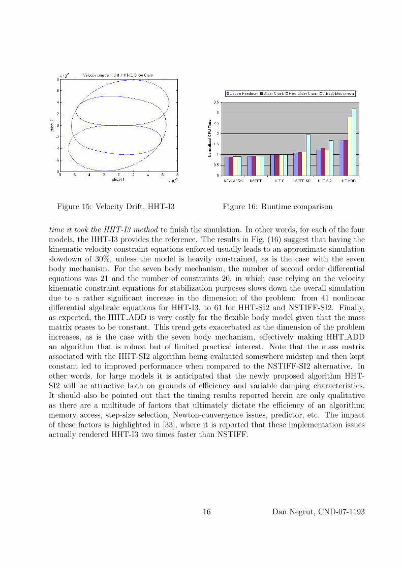
Figure 15: Velocity Drift, HHT-I3 Figure 16: Runtime comparison

time it took the HHT-I3 method to finish the simulation. In other words, for each of the fourmodels, the HHT-I3 provides the reference. The results in Fig. (16) suggest that having thekinematic velocity constraint equations enforced usually leads to an approximate simulationslowdown of 30%, unless the model is heavily constrained, as is the case with the sevenbody mechanism. For the seven body mechanism, the number of second order differentialequations was 21 and the number of constraints 20, in which case relying on the velocitykinematic constraint equations for stabilization purposes slows down the overall simulationdue to a rather significant increase in the dimension of the problem: from 41 nonlineardifferential algebraic equations for HHT-I3, to 61 for HHT-SI2 and NSTIFF-SI2. Finally,as expected, the HHT ADD is very costly for the flexible body model given that the massmatrix ceases to be constant. This trend gets exacerbated as the dimension of the problemincreases, as is the case with the seven body mechanism, effectively making HHT ADDan algorithm that is robust but of limited practical interest. Note that the mass matrixassociated with the HHT-SI2 algorithm being evaluated somewhere midstep and then keptconstant led to improved performance when compared to the NSTIFF-SI2 alternative. Inother words, for large models it is anticipated that the newly proposed algorithm HHT-SI2 will be attractive both on grounds of efficiency and variable damping characteristics.It should also be pointed out that the timing results reported herein are only qualitativeas there are a multitude of factors that ultimately dictate the efficiency of an algorithm:memory access, step-size selection, Newton-convergence issues, predictor, etc. The impactof these factors is highlighted in [33], where it is reported that these implementation issuesactually rendered HHT-I3 two times faster than NSTIFF.


CONCLUSIONS

This paper investigates six low-order numerical integration formulas for determining thetime evolution of constrained multibody systems. The motivation for this effort was twofold.First, the vast majority of large real-life models contain high stiffness, discontinuities, friction,and contacts that effectively make low-order integration formulas the only viable alternativefor numerical simulation. The comparison of these commonly used integration formulasshed light on some advantages and disadvantages associated with each method. Second, thecomparison served as the vehicle that introduced a new integration method, HHT-SI2, andplaced it in the wider family of index 3 and stabilized index 2 methods for the numericalsolution of the DAEs of multibody dynamics.

Compared to higher-order implicit formulas, the numerical methods investigated hereinare robust and straightforward to implement. The algorithms discussed do not have ill-conditioning issues associated with small integration step-sizes due to the suggested scaling,are backed up (with the exception of NEWMARK) by sound theoretical results, and comein two flavors: index-3 and stabilized index-2. Based on the convergence order and timingresults presented, for problems where accurately satisfying the velocity kinematic constraintequations is not a priority, HHT-I3, an algorithm extensively tested and validated on largemodels, represents a good choice. It is a second order method that has the ability to changethe amount of numerical damping that enters the solution process and has recently beenimplemented in the commercial package ADAMS [48]. The NSTIFF method is the nextbest alternative. However, the method is plagued by a somewhat more intense numericaldamping that cannot be controlled like in HHT-I3. For a slower but more robust approach,one can select either HHT-SI2 or NSTIFF-SI2 methods. They are comparable in terms ofefficiency, yet HHT-SI2 has an edge due to (i) its ability to adjust the value of numericaldamping introduced in the solution, and (ii) the handling of the mass matrix, which is boundto lead to efficiency gains for large models. Relative to the simulation times associated withthe straight I3 methods, preliminary results indicate that satisfying both the position andvelocity kinematic constraint equations comes at a price of about a 30% increase in simulationtime.

ACKNOWLEDGEMENTS

This material is based upon work supported by the National Science Foundation underGrant No. CMMI-0700191. Additional financial support was provided by MSC.Software,and, for the first author, by the Wisconsin Space Grant Consortium. The authors wouldlike to thank Radu Serban, Nick Schafer, and Tim Knapp for reading the manuscript andproviding suggestions for improvement, and Toby Heyn for running the convergence ordersimulations for the BDF integrators.


References

[1] Haug, E. J., 1989. Computer-Aided Kinematics and Dynamics of Mechanical SystemsVolume-I. Prentice-Hall, Englewood Cliffs, New Jersey.

[2] Shabana, A. A., 2005. Dynamics of Multibody Systems, third ed. Cambridge UniversityPress.

[3] Abraham, R., and Marsden, J. E., 1985. Foundations of Mechanics. Addison-Wesley.,Reading, MA.

[4] Arnold, V., 1989. Mathematical Methods of Classical Mechanics. Springer, New York,NY.

[5] Brenan, K. E., Campbell, S. L., and Petzold, L. R., 1989. Numerical Solution of Initial-Value Problems in Differential-Algebraic Equations. North-Holland, New York.

[6] Lubich, C., and Hairer, E., 1989. “Automatic integration of the Euler-Lagrange equa-tions with constraints”. J. Comp. Appl. Math., 12, pp. 77–90.

[7] Hairer, E., and Wanner, G., 1991. Solving Ordinary Differential Equations, Vol. II ofComputational Mathematics. Springer-Verlag.

[8] Gear, C. W., 1971. Numerical Initial Value Problems of Ordinary Differential Equations.Prentice-Hall, Englewood Cliffs, NJ.

[9] Bauchau, O., and Laulusa, A., 2008. “Review of Contemporary Approaches for Con-straint Enforcement in Multibody Systems”. Journal of Computational and NonlinearDynamics, 3, p. 011005.

[10] W.C.Rheinboldt, and Potra, F., 1991. “On the numerical solution of euler-lagrangeequations”. Mechanics of structures and machines(19(1)), pp. 1–18.

[11] W.C.Rheinboldt, 1984. “Differential-algebraic systems as differential equations on man-ifolds”. Mathematics of Computation(Vol. 43), pp. 473–482.

[12] Wehage, R. A., and Haug, E. J., 1982. “Generalized coordinate partitioning for di-mension reduction in analysis of constrained dynamic systems”. J. Mech. Design, 104,pp. 247–255.

[13] Liang, C. D., and Lance, G. M., 1987. “A differentiable null-space method for con-strained dynamic analysis”. ASME Journal of Mechanism, Transmission, and Automa-tion in Design, 109, pp. 405–410.

[14] Yen, J., 1993. “Constrained equations of motion in multibody dynamics as odes onmanifolds”. SIAM Journal on Numerical Analysis, 30(2), pp. 553–558.


[15] Alishenas, T., 1992. Zur numerischen behandlungen, stabilisierung durch projectionund modellierung mechanischer systeme mit nebenbedingungen und invarianten,. PhDThesis NASA Technical Memorandum 4760, Royal Institute of Technology, Stockholm.

[16] Mani, N., Haug, E., and Atkinson, K., 1985. “Singular value decomposition for analysisof mechanical system dynamics”. ASME Journal of Mechanisms, Transmissions, andAutomation in Design, 107, pp. 82–87.

[17] Haug, E. J., Negrut, D., and Iancu, M., 1997. “A state-space based implicit integrationalgorithm for differential-algebraic equations of multibody dynamics”. Mechanics ofStructures and Machines, 25(3), pp. 311–334.

[18] Negrut, D., Haug, E. J., and German, H. C., 2003. “An implicit Runge-Kutta methodfor integration of Differential-Algebraic Equations of Multibody Dynamics”. MultibodySystem Dynamics, 9(2), pp. 121–142.

[19] Orlandea, N., Chace, M. A., and Calahan, D. A., 1977. “A sparsity-oriented approachto the dynamic analysis and design of mechanical systems – part I and part II”. Trans-actions of the ASME Journal of Engineering for Industry, pp. 773–784.

[20] Gear, C. W., Gupta, G., and Leimkuhler, B., 1985. “Automatic integration of theEuler-Lagrange equations with constraints”. J. Comp. Appl. Math., 12, pp. 77–90.

[21] Fuhrer, C., and Leimkuhler, B. J., 1991. “Numerical solution of differential-algebraicequations for constrained mechanical motion”. Numerische Mathematik, 59(1), pp. 55–69.

[22] Ascher, U. M., and Petzold, L. R., 1993. “Stability of computational methods forconstrained dynamics systems”. SIAM Journal on Scientific Computing, 14(1), pp. 95–120.

[23] Ascher, U. M., Chin, H., and Reich, S., 1994. “Stabilization of daes and invariantmanifolds.”. Numerische Mathematik, 67(2), pp. 131–149.

[24] Ascher, U. M., Chin, H., Petzold, L., and Reich, S., 1995. “Stabilization of constrainedmechanical systems with DAEs and invariant manifolds.”. Mechanics of Structures andMachines, 23(2), pp. 135–157.

[25] Lubich, C., Nowak, U., Pohle, U., and Engstler, C., 1995. “MEXX - numerical soft-ware for the integration of constrained mechanical multibody systems”. Mechanics ofStructures and Machines, 23, pp. 473–495.

[26] Bauchau, O. A., Bottasso, C. L., and Trainelli, L., 2003. “Robust integration schemes forflexible multibody systems”. Computer Methods in Applied Mechanics and Engineering,192, pp. 395 – 420.


[27] Hughes, T. J. R., 1987. Finite Element Method - Linear Static and Dynamic FiniteElement Analysis. Prentice-Hall, Englewood Cliffs, New Jersey.

[28] Geradin, M., and Rixen, D., 1994. Mechanical Vibrations: Theory and Application toStructural Dynamics. Wiley, New York, NY.

[29] Hilber, H. M., Hughes, T. J. R., and Taylor, R. L., 1977. “Improved numerical dissi-pation for time integration algorithms in structural dynamics”. Earthquake Eng. andStruct. Dynamics, 5, pp. 283–292.

[30] Chung, J., and Hulbert, G. M., 1993. “A time integration algorithm for structural dy-namics with improved numerical dissipation: the generalized-α method”. Transactionsof ASME, Journal of Applied Mechanics, 60(2), pp. 371–375.

[31] Cardona, A., and Geradin, M., 1989. “Time integration of the equation of motion inmechanical analysis”. Computer and Structures, 33, pp. 801–820.

[32] Yen, J., Petzold, L., and Raha, S., 1998. “A time integration algorithm for flexiblemechanism dynamics: The DAE α-method”. Computer Methods in Applied Mechanicsand Engineering, 158, pp. 341–355.

[33] Negrut, D., Rampalli, R., Ottarsson, G., and Sajdak, A., 2007. “On the use of theHHT method in the context of index 3 Differential Algebraic Equations of MultibodyDynamics”. ASME Journal of Computational and Nonlinear Dynamics, 2.

[34] Arnold, M., and Bruls, O., 2007. Convergence of the generalized-α scheme for con-strained mechanical systems. Tech. Rep. 9-2007, Martin Luther University, FachbereichMathematik und Informatik, Halle-Wittenberg.

[35] Lunk, C., and Simeon, B., 2006. “Solving constrained mechanical systems by the familyof Newmark and α-methods”. ZAMM, 86, pp. 772–784.

[36] Jay, L. O., and Negrut, D., 2007. “Extensions of the HHT-α method to Differential-Algebraic Equations in mechanics”. Electronic Transactions on Numerical Analysis,26, pp. 190–208.

[37] Jay, L. O., and Negrut, D., 2008. “A second order extension of the generalized-α methodfor constrained systems in Mechanics”. in preparation.

[38] Bottasso, C. L., Bauchau, O. A., and Cardona, A., 2007. “Time-step-size-independentconditioning and sensitivity to perturbations in the numerical solution of index threedifferential algebraic equations”. SIAM Journal on Scientific Computing, 3, pp. 395–420.

[39] Newmark, N. M., 1959. “A method of computation for structural dynamics”. Journalof the Engineering Mechanics Division, ASCE, pp. 67–94.


[40] Schiehlen, W., ed., 1990. Multibody Systems Handbook. Springer.

[41] Hairer, E., and Wanner, G., 1996. Solving Ordinary Differential Equations II: Stiff andDifferential-Algebraic Problems. Springer.

[42] Khude, N., and Negrut, D., 2007. A MATLAB implementation of the seven-bodymechanism for implicit integration of the constrained equations of motion. Tech. Rep.TR-2007-07, Simulation-Based Engineering Laboratory, The University of Wisconsin-Madison.

[43] Lotstedt, C., and Petzold, L., 46. “Numerical solution of nonlinear differential equationswith algebraic constraints I: Convergence results for backward differentiation formulas”.Mathematics of Computation, 174, pp. 491–516.

[44] Brenan, K., and Engquist, B. E., 1988. “Backward differentiation approximationsof nonlinear differential/algebraic systems”. Mathematics of Computation, 51(184),pp. 659–676.

[45] Negrut, D., Jay, L., Khude, N., and Heyn, T., 2007. “A discussion of low-order integra-tion formulas for rigid and flexible multibody dynamics”. In Proceeding of MultibodyDynamics ECCOMAS Thematic Conference.

[46] Schafer, N., Negrut, D., and Serban, R., 2008. Experiments to compare implicit andexplicit methods of integration in molecular dynamics simulation. Tech. Rep. TR-2008-01, Simulation-Based Engineering Laboratory, The University of Wisconsin-Madison.

[47] Khude, N., Jay, L. O., and Negrut, D., 2008. A comparison of low order numericalintegration formulas for rigid and flexible multibody dynamics. Tech. Rep. TR-2008-02,Simulation-Based Engineering Laboratory, The University of Wisconsin-Madison.

[48] MSC.Software, 2005. ADAMS User Manual: http://www.mscsoftware.com.


a discussion of low order numerical integration formulas for...

Documents