A Discrete Choice Model of Transitions to Sustainable Technologies

Paolo Zeppini

No. 28 /14

BATH ECONOMICS RESEARCH PAPERS

Department of Economics

A Discrete Choice Model of Transitionsto Sustainable Technologies∗

Paolo Zeppini

Department of Economics, University of Bath, UKCeNDEF, Amsterdam School of Economics, University of Amsterdam, The Netherlands

Istituto di Economia, Scuola Superiore Sant’Anna, Pisa

Abstract

We propose a discrete choice model of sustainable transitions from dirty to cleantechnologies. Agents can adopt one technology or the other, under the influence ofsocial interactions and network externalities. Sustainable transitions are addressedas a multiple equilibria problem. A pollution tax can trigger a sudden transition asa bifurcation event, at the expenses of large policy efforts. Alternatively, periodicdynamics can arise. Technological progress introduced in the form of endogenouslearning curves stands as a fundamental factor of sustainable transitions. For this towork, the positive feedback of network externalities and social interaction should bereduced initially, for instance by promoting niche markets of clean technologies andmaking technological standards and infrastructure more open. Traditional policychannels such as pollution tax and feed-in-tariffs have an auxiliary - yet important- role in our model. Compared to feed-in-tariffs, a pollution tax promotes smootherand faster transitions.

Key words: bounded rationality, environmental policy, learning curves, multiple equilibria,network externalities, social interactions.

JEL classification: C62, D62, O33, Q55

1 Introduction

Resource scarcity, climate change and environmental justice are among the major chal-

lenges faced by human mankind in present times. These challenges require profound

changes of industrial and agricultural sectors, but also involve behaviours, institutions

and more generally the organization of society. In particular environmental challenges

call to reform energy, housing, and transportation, and pose new targets for technological

progress towards sustainable solutions (van den Bergh, 2012).

∗The author is grateful to Cars Hommes, Jeroen van den Bergh and Koen Frenken for useful discus-sions. The article benefited from useful comments by participants at Tinbergen Institute PhD seminarseries in Amsterdam, the EAERE 2012 conference in Prague and the WCERE 2014 congress in Istanbul.

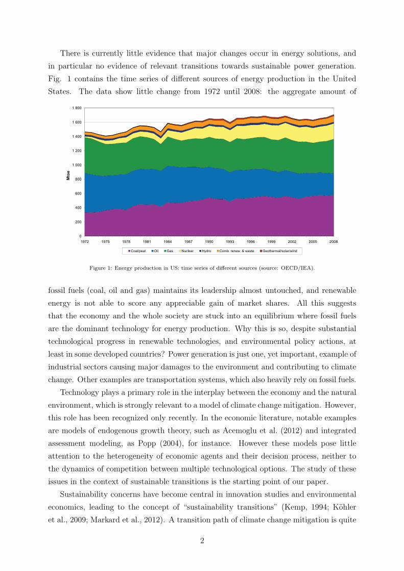
There is currently little evidence that major changes occur in energy solutions, and

in particular no evidence of relevant transitions towards sustainable power generation.

Fig. 1 contains the time series of different sources of energy production in the United

States. The data show little change from 1972 until 2008: the aggregate amount of

1 200

1 400

1 600

1 800

0

200

400

600

800

1 000

1972 1975 1978 1981 1984 1987 1990 1993 1996 1999 2002 2005 2008

Mtoe

Coal/peat Oil Gas Nuclear Hydro Comb. renew. & waste Geothermal/solar/wind

Figure 1: Energy production in US: time series of different sources (source: OECD/IEA).

fossil fuels (coal, oil and gas) maintains its leadership almost untouched, and renewable

energy is not able to score any appreciable gain of market shares. All this suggests

that the economy and the whole society are stuck into an equilibrium where fossil fuels

are the dominant technology for energy production. Why this is so, despite substantial

technological progress in renewable technologies, and environmental policy actions, at

least in some developed countries? Power generation is just one, yet important, example of

industrial sectors causing major damages to the environment and contributing to climate

change. Other examples are transportation systems, which also heavily rely on fossil fuels.

Technology plays a primary role in the interplay between the economy and the natural

environment, which is strongly relevant to a model of climate change mitigation. However,

this role has been recognized only recently. In the economic literature, notable examples

are models of endogenous growth theory, such as Acemoglu et al. (2012) and integrated

assessment modeling, as Popp (2004), for instance. However these models pose little

attention to the heterogeneity of economic agents and their decision process, neither to

the dynamics of competition between multiple technological options. The study of these

issues in the context of sustainable transitions is the starting point of our paper.

Sustainability concerns have become central in innovation studies and environmental

economics, leading to the concept of “sustainability transitions” (Kemp, 1994; Kohler

et al., 2009; Markard et al., 2012). A transition path of climate change mitigation is quite

2

different from a gradual and linear path, with strong implications for macroeconomic

theory and environmental policy (van der Ploeg, 2011). Moreover, the intrinsic dynamic

nature of a transition event finds a natural conceptual framework in evolutionary mod-

elling (Foxon, 2011).

Sustainability transitions often imply a regime shift from an established technology to

an innovative technology. The idea of technological regime is central to transition thinking

and to evolutionary economics (Nelson and Winter, 1982). A technological regime has

often the connotation of “lock-in” (Arthur, 1989). A technological lock-in is a state in

which one technology is dominant in a particular application domain or industrial sector,

and competing alternatives find it hard if not impossible to enter the market, even if they

are socially desirable (David, 1985).

Technological lock-in is the result of increasing returns to adoption: a technology

tends to be more attractive the more it is adopted. Several factors give place to this

positive externality in adoption decisions: learning effects among producers and users, the

advantages of common standards and infrastructure, and the provision of complementary

goods, services and institutions. These factors add to the utility of using a technology and

in economics are often referred to as “network externalities” (Katz and Shapiro, 1985).

Network externalities give rise to barriers which are strong to be broken. This scenario

translates into multiple equilibria, and once the economy is stuck in one of those, with

one technology dominating the market (technological lock-in), it is hard for alternative

technologies to gain market shares, let alone to overcome the dominant technology. In

the energy sector, a shift from the equilibrium represented by fossil fuels is very hard to

achieve, due to the large scale of infrastructures and amount of investments, a fact that

suggested the notion of “carbon lock-in” (Unruh, 2000; Konnola et al., 2006). A possible

way to escape carbon lock-in has been analysed by Zeppini and van den Bergh (2011)

with the concept of “recombinant innovation”.

There are other sources of positive feedback, beside network externalities, which stem

from social interactions in the form of imitation and social learning (Young, 2009), confor-

mity effects and habit formation (Alessie and Kapteyn, 1991), or even forms of recruitment

(Kirman, 1993). In this paper we propose an analytical framework for the study of sus-

tainability transitions based on discrete choice dynamics, building on social interactions

models such as Brock and Durlauf (2001).

We frame the transition to sustainable technologies as a coordination problem with

multiple equilibria. There is growing evidence of the explanatory power of behavioural

approaches to an incrising variety of economic contexts (de Grauwe, 2012; Hommes, 2013).

These approaches have largely missed to address environmental problems so far. Never-

theless, behavioural concepts such as bounded rationality of agents and their switching

3

behaviour are quite relevant to the issue of sustainability transition, as we show in the

present article. The main point of our analysis is the role of decision externalities within

the dynamics of sustainability transitions and the resulting equilibrium structure.

In the second part of the article we extend our discrete choice model of competing

technologies in two directions, namely environmental policy and technological progress.

We model technological progress as a cumulative process that depends endogenously on

past agents’ adoption decisions. By making technology explicit, we can introduce different

policy channels, such as R&D subsidies to stimulate sustainable choices beside taxes on

polluting technologies. We address a simple scenario with the competition between a

“clean” and a “dirty” technology, and an environmental policy attempting to promote

the former. Such policy can trigger a transition to clean technologies - a sustainability

transition - by affecting the dynamics of the decision system and its equilibria.

Our model gives the following indications: a static policy that misses to focus on

technological progress, such as a pollution tax, can only marginally reduce the share of

a dirty technology, and can trigger a major transition only with an equilibrium shift, at

the expense of relatively large efforts. A policy that favours technological progress for

the clean solution can foster smooth and continuous transitions. However, in a scenario

where the dirty technology is initially dominant the clean technology is strongly opposed

by the positive feedback of network externalities and social interactions.

The main message of the extended version of the model is the role of positive feedback

in shaping the pattern of technological progress itself for two competing options, which in

turn determines the fate of a possible sustainability transition. Beside pollution taxes and

R&D subsidies, an effective policy should control the positive feedback of decision exter-

nalities. In doing this, undesirable equilibria such as a carbon lock-in could be attacked

by lowering the barriers to the adoption of sustainable technologies, thus promoting a

transition to a self-sustaining equilibrium where sustainable technologies are dominant.

The structure of this article is as follows. Section 2 presents a basic version of the

model. Section 3 introduces environmental policy. Section 4 extends the model with

technological progress. Section 5 brings together environmental policy and technological

progress. Section 6 concludes.

2 Social interactions and network externalities

Consider M technologies competing in the market for adoption or for R&D investment

by N agents (N � M). The utility, or profitability, from technology c in period t is

uc,t = λc + ρcxc,t, (1)

4

where λc is the profitability of technology c, and xc,t is the fraction of agents that choose

technology c in period t. For the moment we assume λc to be constant, that is we

discard technological progress. In Section 4 we relax this assumption. The parameter

ρc > 0 expresses the intensity of positive externalities in agents’ decisions. The term

ρcxc,t describes the self-reinforcing effect of decision externalities. There may be cases

where social interactions give place to negative feedback, as with conspicuous consumption

aiming at social status. We discard this possibility here, and consider social interactions

together with network externalities as a unique source of self-reinforcement in technology

adoption decisions.

We adopt the discrete choice framework of Brock and Durlauf (2001). The general case

with M choice options is addressed in Brock and Durlauf (2002) and in Brock and Durlauf

(2006). According to this model, each agent i experiences a random utility ui,t = ui,t+εi,t,

where the noise εi,t is iid across agents, and it is known to an agent at the decision time t.

In the limit of an infinite number of agents, when the noise εi,t has a double exponential

distribution, the probability of adoption of technology c converges to the Gibbs probability

of the multinomial logit model:

xc,t =eβuc,t−1

∑Mj=1 e

βuj,t−1

. (2)

The parameter β is the intensity of choice and it is inversely related to the variance of the

noise εi,t (Hommes, 2006). In the limit β → 0 the different technologies tend to an equal

share 1/M . The limit β → ∞ represents the “rational agent” limit, where everybody

chooses the optimal technology.

In the context of our model, an agent who is confronted with the technology choice

knows only with limited precision the decisions of other agents and the benefits associated

with them, that is the social term ρcxc,t of Eq. (1). Our model differs from Brock and

Durlauf (2001) in the following: we do not model expectations about dynamic variables

explicitly, and the choice that agents face is not one among different predictors, but a

choice between technological options with different profitability λj in Eq. (1). An agent’s

decision is based on past experience, namely the knowledge of the market penetration of

technologies in the last period. This is where the only dynamic variable of the model, the

fraction xt, enters the decision mechanism, either as technological network externalities

or in temrs of social interactions. Moreover, our focus is on the dynamics of technology

competition, and on their different attractors other than a stable equilibrium. Such focus

calls for using the discrete choice framework as a model of decision dynamics (2), similarly

to Brock and Hommes (1997), rather than a condition for equilibrium consistency, like in

Brock and Durlauf (2001). In this way we model the switching behaviour of technology

competition. A model proposed by Smallwood and Conlisk (1979) considers a similar

5

switching mechanism where consumers take into account the market share of products,

beside their quality. The main difference of our model is that we make explicit the

dynamics of choices.

Consider the simplest scenario with two competing technologies, labelled c and d.

This model is one-dimensional: one state variable, the fraction of technology c, xc ≡ x,

is enough for knowing the state of the system at a given time (xd = 1 − x). Assume for

simplicity an equal increasing return on adoption ρc = ρd ≡ ρ for the two technologies.

The difference of utilities is central in this model:

ud,t − uc,t = λ+ ρ(1− 2xt), (3)

where λ ≡ λd − λc is the difference in profitability between the two technologies. The

probability of adoption (and the market share) of technology c in period t is:

xt =eβ(λc+ρxt−1)

eβ(λc+ρxt−1) + eβ[λd+ρ(1−xt−1)]=

1

1 + eβ[λ+ρ(1−2xt−1)]≡ f(xt−1). (4)

Analytical results regarding the dynamics of the system (4) are in line with Brock and

Durlauf (2001). The fixed points of the map f give the equilibrium values for xt.

Proposition 1 The system (4) has either one stable steady state or an unstable steady

state x∗ and two stable steady states x∗1 and x∗

2 such that x∗1 ≤ x∗ ≤ x∗

2.

0 0.2 0.4 0.6 0.8 10

0.1

0.2

0.3

0.4

0.5

0.6

0.7

0.8

0.9

1

x

f(x)

λ = 0

β = 1

β = 2

β = 3.4β = 10β = 5

0 0.2 0.4 0.6 0.8 10

0.1

0.2

0.3

0.4

0.5

0.6

0.7

0.8

0.9

1

x

f(x)

λ = 0.2

β = 1

β = 2β = 3.4

β = 10β = 5

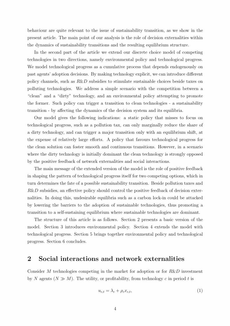
Figure 2: Map f for different values of β (ρ = 1). Left: equally profitable technologies (symmetric case).

Right: technology d more profitable than c (asymmetric case).

A first observation is that x = 0 and x = 1 (technological monopoly) are equilibria only

for β = ∞, which represents the limit of perfect rationality in agents’ decision. For finite

β the technology with lower profitability never disappears. Fig. 2 shows some examples

with different values of β for λ = 0 and λ = 0.2 (with ρ = 1). In the symmetric case

λ = 0 (left panel) the steady state x = 1/2 is stable if f ′(1/2) ≤ 1, which is true if β ≤ 2.

Whenever the intensity of choice is smaller than 2, the adoption process will converge to

equal shares of technologies c and d. Conversely, for β > 2 the system converges to one

6

of two alternative steady states, where one technology is dominant. The critical value

(β = 2) is the bifurcation value. Symmetry of the two technologies (λ = 0) gives place to

a “pitchfork bifurcation” for β = 2, where the steady state x = 12loses stability and two

new stable steady states are created. This is the case in the example of the left panel of

Fig. 2, for a value of β between 2 and 3.

When one technology is more profitable than the other (λ �= 0), the intensity of

choice β and the returns on adoption ρ play a different role in Eq. (4), and additional

steady states are created by a “tangent bifurcation”.1 The right panel of Fig. 2 shows

a tangent bifurcation for β � 3.4, in which two steady states are created, one stable

and one unstable. For more examples on the role of β and ρ see Zeppini (2011). Fig.

3 (left panel) describes the qualitative changes in dynamics brought by changes in the

differential profitability λ. No pitchfork bifurcations take place for this parameter, but

0 0.2 0.4 0.6 0.8 10

0.2

0.4

0.6

0.8

1

x

f(x)

λ = −0.2λ = 0λ = 0.2

ρ = 0.1

0 0.2 0.4 0.6 0.8 10

0.2

0.4

0.6

0.8

1

x

f(x)

λ = −0.2λ = 0λ = 0.2

ρ = 0.5

0 0.2 0.4 0.6 0.8 10

0.2

0.4

0.6

0.8

1

x

f(x)

λ = −0.2λ = 0λ = 0.2

ρ = 1

Figure 3: Map of the model (Eq. 4) for different values of the difference in profitability λ and the

intensity of externalities ρ. Left: ρ = 0.1. Centre: ρ = 0.5. Right: ρ = 1. Here β = 4.

tangent bifurcations are possible if ρ or β are large enough. The left panel of Fig. 3

indicates that such a bifurcation occurs for λ slightly larger than 2 in absolute value. It

is remarkable that in the asymmetric case λ �= 0 the less profitable technology (lower λj,

with j = c, d) may attain a larger share in equilibrium. A positive value of λ (technology

d better than c), for instance, shifts the map to the right, with an unstable steady state

x∗ > 1/2. If the initial condition x0 > x∗ > 12, the system converges to x∗

2, with a larger

share of technology c, despite this one being worse than technology d.

Fig. 4 reports the bifurcation diagram of λ for three different values of ρ. When

externalities are weak (left panel) the transition from one to the other technology driven by

a change in the difference of profitability values is smooth. As the intensity of externalities

1In this version of the model the number of parameters could be reduced to two: λ = βλ, and ρ = βρ.

We still use three distinct parameters in order to better compare our model to the literature, with β

having an important role in discrete choice and bounded rationality models (Brock and Hommes, 1997),

and ρ in social interactions with discrete choice models (Brock and Durlauf, 2001). A second reason for

using three distinct parameters is that in Section 4 we extend the model with a learning curve for λ.

7

−1 −0.5 0 0.5 10

0.2

0.4

0.6

0.8

1

λ

x

−1 −0.5 0 0.5 10

0.2

0.4

0.6

0.8

1

λ

x

−1 −0.5 0 0.5 10

0.2

0.4

0.6

0.8

1

λ

x

Figure 4: Bifurcation diagram of the difference in profitability λ for three different values of the intensity

of externalities ρ. Left: ρ = 0.1. Centre: ρ = 0.5. Right: ρ = 1. Here β = 4, x0 = 0.5.

becomes larger, the transition becomes more abrupt, but it is still continuous. Above a

certain a level of ρ (pitchfork bifurcation) the transition takes the connotation of a jump

(right panel). In this scenario there is not one equilibrium anymore, but two alternative

equilibria. As the difference in profitability turns in favour of one technology, agents jump

massively from one equilibrium to the other.

The values of β, ρ and λ together determine the steady states of the system and its

dynamics. In particular, these parameters set the conditions for multiple equilibria. The

following two necessary conditions hold true:

Proposition 2 ρβ > 2 and −ρ < λ < ρ are necessary conditions for multiple equilibria.

The proof is based on the position of the inflection point x = λ+ρ2ρ

of the map f and on the

maximum derivative f ′(x) = βρ2

(see Appendix A). The general message of Propositions

1 and 2 nicely match results obtained by Antoci et al. (2014) with their evolutionary

game model of firms facing innovation decisions in the context of the Emission Trading

System. This match testifies how the various implications of multiple equilibria are a

robust property of the dynamics of adoption decision problems.

The intensity of choice regulates the shape of the map (4): the larger is β, the more

f is similar to a step function, with a discontinuity in x = λ+ρ2ρ

. The following holds true:

Proposition 3 Consider map (4):

• when β ≈ 0, there is a unique equilibrium, and it is stable.

• when β ≈ ∞, there may be three cases:

1. if λ < −ρ the equilibrium x∗2 = 1 is unique and stable,

2. if λ > ρ the equilibrium x∗1 = 0 is unique and stable,

3. if −ρ < λ < ρ, x∗ = x = λ+ρ2ρ

is unstable, while x∗1 = 0 and x∗

2 = 1 are stable.

8

The proof of Proposition 3 relies on the fact that when β = ∞, the two conditions of

Proposition 2 are also sufficient for multiple equilibria, because the system depends only

on the position of the inflection point x; in the third case, x falls inside the interval [0, 1],

and both x = 0 and x = 1 are stable equilibria. In this case the market will be completely

taken by one or the other technology, depending on the initial condition.2

3 Competing technologies and environmental policy

We now move to the realm of sustainability transitions, and consider technologies that

have a direct impact on the natural environment which can be described by a measure

of pollution emission intensity. Environmental policies favour less polluting technologies.

The actual economy is characterized by many instances of dirty incumbent technologies

and innovative clean technologies that find it hard to break through and gain substantial

market shares. One example is power generation, where fossil-fuels are dominant, and

renewable energy is still marginal (Fig. 1). A sustainable transition in this case would

be a shift from fossil fuels to renewables. Without policy intervention, this is unlikely

to happen, due to the larger profitability of the former. In this section we study the

conditions for an environmental policy to trigger such a transition.

Let d be a “dirty” technology, with high pollution intensity (e.g. fossil fuels) and

c a “clean” technology, with low pollution intensity (e.g. solar Photo-Voltaic). Let’s

assume the clean technology has higher production costs (or lower performance), which

translates into a profitability gap λ = λd − λc > 0. The goal of an environmental policy

is to make λ low enough, so as to eliminate the less desirable equilibrium, or to promote

the coordination of decision makers in the alternative desirable equilibrium (Fig. 3).

In the case of power generation, environmental policies aim at the “grid parity”, where

clean energy (solar, wind) reaches the cost (and the profitability) of traditional energy

sources (fossil fuels). Different policies have been implemented in different countries (Fis-

cher and Newell, 2008), which either impose taxes on pollution or provide market subsidies

for the clean(er) technology. Taxes make the dirty technology more expensive, by inter-

nalizing the pollution externality. Subsidies make the clean technology less expensive.

Both measures result in an attempt to lower the profitability gap λ. Here we extend the

model of competing technologies with a pollution tax.

Environmental policies tend to be endogenous to technology competition, because their

effort usually decreases as the share of the clean technology increases. We introduce a tax

τ(1 − x) charged on the adoption of the dirty technology. This tax term is proportional

2If we add an arbitrarily small noise term to the state variable x, our model replicates results in Arthur

et al. (1987), as shown in Zeppini (2011), Chapter 4.

9

to the market share of the dirty technology, with constant tax rate τ . If we assume a

constant installed capacity of production from clean and dirty technologies together, and

a constant pollution intensity for the dirty technology, this policy works as a tax on the

average pollution emission. The profitability gap is reduced by τ(1−x), and the difference

of utility from dirty and clean technologies becomes:

ud,t − uc,t = λ0 + ρ(1− 2xt)− τ(1− x), (5)

where λ0 = λd − λc is the profitability gap without policy. The map of the system is:

fτ (x) =1

1 + eβ[λ0+ρ(1−2x)−τ(1−x)]. (6)

The dynamics of the share of clean technology is given by xt = fτ (xt−1). Without policy

(τ = 0) one is back to the basic model (4). The pollution tax introduces a negative

feedback that counters the positive feedback of network externalities in agents’ adoption

decisions. Notice that a pollution tax is formally equivalent to a subsidy for the clean

technology in a model such as ours, which limits its scope of analysis to the relative shares

dynamics of a system of competing technologies.3

A pollution tax enlarges the basin of attraction of the “clean” equilibrium at the ex-

penses of the basin of the “dirty” equilibrium. However only the latter remains populated,

if the initial condition belongs to this one, as it is often the case in reality. A transition

does not occur, due to the lack of coordination. The pollution tax may trigger an abrupt

shift to the “clean” equilibrium, if τ reaches a threshold value where the “dirty” equi-

librium ceases to exist (bifurcation), and agents are forced to coordinate on the “clean”

equilibrium. This means that a transition to clean technologies with such a policy occurs

with an ever increasing (and socially expensive) stringency, and only realizes through a

sudden regime shift. Both features are possibly unattractive and unfeasible. A smoother

transition requires dynamically changing adaptive factor, such as technological progress,

and possibly a dynamic environmental policy, as we show in Section 4 and Section 5.

A change in the number of stable equilibria is not the only qualitative effect of a

pollution tax. In particular, it can lead to cyclical dynamics. The following lemma holds:

Lemma 1 A necessary condition for cyclical dynamics is τ > 2ρ.

The proof of Lemma 1 is in Appendix A. The inequality τ > 2ρ is a condition for a

downward sloping map. In order to have cyclical dynamics the initial profitability gap

plays a role, as stated by the following proposition:

3In a general equilibrium setting, taxes and subsidies have substantially different impacts on the

economy. For instances, taxes limit overall consumption, while subsidies foster it. Nevertheless, the effect

on the adoption of clean technologies stays the same as in our partial equilibrium analysis.

10

Proposition 4 There are six cases:

1. the map fτ is upward sloping (τ < 2ρ):

(a) λ0 < ρ: a larger τ increases the share of clean technology in equilibrium, and

leads to a tangent bifurcation. The inflection point is x < 1.

(b) λ0 = ρ: there is only one steady state, which is stable. The inflection point is

x = 1.

(c) λ0 > ρ: there is only one steady state, which is stable. The inflection point is

x > 1.

2. the map fτ is downward sloping (τ > 2ρ):

(a) λ0 < ρ: there is only one steady state, which is stable. A larger τ increases the

equilibrium share. The inflection point is x > 1.

(b) λ0 = ρ: there is only one steady state, which becomes unstable for τ sufficiently

large, giving place to a stable period 2 cycle. The inflection point is x = 1.

(c) λ0 > ρ: there is only one steady state, which becomes unstable for τ sufficiently

large, giving place to a stable period 2 cycle. The inflection point is x < 1.

The proof is in Appendix A. The intuition for cyclical dynamics of technology shares is

the following. An environmental policy that reduces the profitability gap as indicated by

Eq. (5) introduces a negative feedback, which opposes the positive feedback of network

externalities. These two forces can balance each other leading to a stable equilibrium. But

if the tax rate is too high, the negative feedback of environmental policy overcomes the

positive feedback of network externalities. As soon as the profitability gap is reduced, the

policy intervention for the next period is reduced accordingly (Eq. 5). The profitability

gap widens again, calling for the policy to be re-enforced, and the story repeats. Fig. 5

illustrates the different cases of Proposition 4 with a number of examples. A tougher policy

0 0.2 0.4 0.6 0.8 10

0.2

0.4

0.6

0.8

1

x

f(x)

τ = 3τ = 2τ = 1.5

τ = 1

τ = 0.6

τ = 0.2

τ = 0

ρ = 0.1

0 0.2 0.4 0.6 0.8 10

0.2

0.4

0.6

0.8

1

x

f(x)

τ = 3τ = 2

τ = 1.5

τ = 1

τ = 0.6

τ = 0.2

τ = 0

ρ = 0.5

0 0.2 0.4 0.6 0.8 10

0.2

0.4

0.6

0.8

1

x

f(x)

τ = 3τ = 2

τ = 1.5τ = 1

τ = 0

τ = 0.2µ

ρ = 1

Figure 5: Competing technologies and environmental policy. Map fτ for seven different values of

pollution tax τ and three levels of network externalities ρ. (Here λ0 = 0.5 and β = 6)

11

(larger τ) generally leads to a larger share of clean technology, as one may expect. Beyond

a threshold value of τ cyclical dynamics occur. Both effects are clear in the left and middle

panels of Fig. 5. In the left panel (λ0 > ρ, cases (1c) and (2c) of Proposition 4) there is

always a unique steady state, and an increasing effort shifts the inflection point x to the

right. In the middle panel (λ = ρ, cases (1b) and (2b)) there is still only one steady state,

but the inflection point position x = 1 is unaffected. In the right panel (λ0 < ρ, cases (1a)

and (2a)), rising τ leads to a tangent bifurcation for τ � 0.6, with the appearance of two

additional steady states, one of which stable. Another tangent bifurcation above τ = 1

reduces the number of steady states again to only one. We can resume the effect of the

environmental policy in the condition of the right panel as follows: for low effort values

the marginal effect of the policy on the market share of the clean technology is very small,

and the system is stuck into the only stable equilibrium where the dirty technology is

dominant. For middle values of the effort, the environmental policy creates an alternative

stable equilibrium where the clean technology is dominant. However, such equilibrium

is still unpopulated. Higher efforts lead to a sudden shift, eliminating the suboptimal

equilibrium. If the economy is locked-in into a dirty technology, this event tips the market

towards the clean technology. Concluding, the positive feedback of network externalities

and social interactions gives multiple equilibria and technological lock-in. When this

positive feedback is relatively weak, an environmental policy can increase the share of

the clean technology. But if the policy effort is too strong it destabilizes the market with

cyclical dynamics. Fig. 6 on the left reports a simulated time series of the share xt that

converges to a period 2 cycle. The right panel of Fig. 6 is a bifurcation diagram of the tax

0 10 20 30 400.1

0.2

0.3

0.4

0.5

0.6

0.7

0.8

0.9

1

t

x

0 1 2 3 4 50

0.2

0.4

0.6

0.8

1

τ

x

Figure 6: Competing technologies and environmental policy. Left: time series of the share of clean

technology. Right: bifurcation diagram of τ . λ0 = 1.5, ρ = 1, β = 4 and τ = 4 (left).

rate τ . By comparing the left and right panels of Fig. 5 we see that a lower intensity of

positive feedback from network externalities and social interactions makes it more likely

for an environmental policy to fall into cyclical dynamics.

A periodic attractor is possibly not a realistic outcome, but in the present analysis

12

it unveils the limits of a policy that only looks at reducing the relative shares of a dirty

technology. Such policy fails in establishing effectively a decision environment that favours

the clean technology, since it just creates temporary (periodic) incentives for it. An

effective policy would be one that structurally changes the decision environment by closing

the profitability gap λ. This is achieved trhough technological change, as we show in

Section 4. The main message from this analysis, that is contained in Fig. 5, is that

in the case of a relatively weak positive feedback from social interactions and network

externalities, where the barriers to a clean solution would be easier to cross, the unwanted

outcome of a periodic dynamics following is actually more likely.

The switching behaviour of the discrete choice framework may be unrealistic in cases

where large sunk costs cause stickiness in the decision process. The power generation

sector is an example, where the choice of energy resource is limited. The discrete choice

framework allows to introduce persistence of behaviours through asynchronous updating

(Diks and van der Weide, 2005; Hommes et al., 2005). This extension of the model

responds to the idea that not all agents update their strategy in every period. The

discrete choice model with asynchronous updating is given by

xi,t = αxi,t−1 + (1− α)eβui,t−1

∑Mj=1 e

βuj,t−1

, (7)

where α is the portion of agents that stick to their previous strategy, while a fraction

1 − α chooses a strategy based on the discrete choice mechanism (2). A larger α gives

more persistence of strategies.

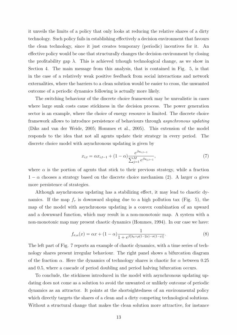
Although asynchronous updating has a stabilizing effect, it may lead to chaotic dy-

namics. If the map fτ is downward sloping due to a high pollution tax (Fig. 5), the

map of the model with asynchronous updating is a convex combination of an upward

and a downward function, which may result in a non-monotonic map. A system with a

non-monotonic map may present chaotic dynamics (Hommes, 1994). In our case we have:

fσ,α(x) = αx+ (1− α)1

1 + eβ[λ0+ρ(1−2x)−σ(1−x)]. (8)

The left part of Fig. 7 reports an example of chaotic dynamics, with a time series of tech-

nology shares present irregular behaviour. The right panel shows a bifurcation diagram

of the fraction α. Here the dynamics of technology shares is chaotic for α between 0.25

and 0.5, where a cascade of period doubling and period halving bifurcation occurs.

To conclude, the stickiness introduced in the model with asynchronous updating up-

dating does not come as a solution to avoid the unwanted or unlikely outcome of periodic

dynamics as an attractor. It points at the shortsightedness of an environmental policy

which directly targets the shares of a clean and a dirty competing technological solutions.

Without a structural change that makes the clean solution more attractive, for instance

13

0 10 20 30 40

0.4

0.5

0.6

0.7

0.8

0.9

1

t

x

0 0.2 0.4 0.6 0.8 10

0.2

0.4

0.6

0.8

1

α

x

Figure 7: Environmental policy and asynchronous updating. Left: time series of x. Right: bifurcation

diagram of α. Here λ0 = 2, ρ = 1, τ = 9, β = 5 and α = 0.3 (left).

by increasing its profitability λc, such policy may easily end up with promoting irregular

behaviours by decision makers with consequent irregular patterns of technology shares.

4 Competing technologies and technological progress

In this section we extend the discrete choice model of technology competition of Section

2 by introducing an endogenous mechanism of technological progress. The stream of

research that goes under the name of “endogenous growth theory” addresses the mutual

relationship between economic growth and technological progress (Romer, 1990; Aghion

and Howitt, 1998; Acemoglu, 2008). The main feature of this approach to economic growth

is the recognition of mutual effects between the economy and technological change, going

beyond the traditional one-way relationship from science to technology to the economy.

Although these models are generally claimed to have micro-foundations, relatively little

attention is given to the decision of agents concerning which technology to adopt. The role

of agency in technological change has recently been the main focus of a number of agent-

based models, as for instance Andergassen et al. (2009), Cantono and Silverberg (2009),

van der Vooren A. (2012) and Frenken et al. (2012). Here we take a behavioural angle in

the description of technological change (Hommes and Zeppini, 2014) that links these two

approaches, and study the decision process that underlies the interplay of technological

competition and technological progress. Building on the discrete choice mechanism of

the model in Section 2, we can study in particular how network externalities and social

interactions shape technological progress.

Consider again two competing technologies c and d with utility given by (1). Now

we relax the hypothesis of constant profitabilities λc and λd. Assume that technological

progress for c and d depends on the cumulative investment in the two technologies, for

14

instance R&D investment, and in every period the invested amounts are proportional to

market shares, with a constant coefficient of proportionality. We also assume that tech-

nological progress is concave in technological investments, in line with endogenous growth

models (Aghion and Howitt, 1998; Barlevy, 2004). Resuming, we model technological

progress with the following learning curves:

λc,t = λc0 + ψc

( t∑

j=1

xj

)ζ

, λd,t = λd0 + ψd

( t∑

j=1

(1− xj)

)ζ

, (9)

with λc0 and λd0 the profitabilities without technological progress. The sum series rep-

resent the cumulation of each period investments, from j = 1 to the present time j = t.

The difference in profitability values is now a technological gap:

λt = λd,t − λc,t = λ0 + ψd

( t∑

j=1

(1− xj)

)ζ

− ψc

( t∑

j=1

xj

)ζ

, (10)

where λ0 is the technological gap without progress. ψc, ψd measure how investment trans-

lates into technological progress. ζ ∈ [0, 1] dictates the curvature of the learning function.

This parameter is likely to be different for different technologies, but in a first order

approximation we assume the same value for the two competing technologies.

The difference in utility between technology d and technology c equipped with the

learning curves above becomes:

ud,t − uc,t = λt + ρ(1− 2xt), (11)

Here technology competition is driven both by externalities (the second term of the right

hand side) and technological progress (the first term): the share of technology c according

to (2) is now given by:

xt =1

1 + eβ[λt−1+ρ(1−2xt−1)]≡ ft−1(xt−1). (12)

The map ft−1 depends on time. It is identical to the map f of the basic model (4) after

substituting the static parameter λ with the time varying technological gap of Eq. (10).

Endogenous technological progress as expressed by the dynamic technological difference λt

is a slowly changing parameter that modifies the flow map of the competing technology

system as shown in Fig. 3. The long run dynamic of this system is obtained with

the limit map set by the value limt→∞ λt ≡ λ∞. The technology gap λ may affect the

number of stable equilibria by shifting the map, although it does not modify its shape

(See Proposition 2). There can be two cases:

1. if the steady state x∗ of Proposition 1 is stable, a change in λ changes gradually the

equilibrium market shares as one technology slowly catches up (Fig. 3, left panel);

15

2. if x∗ is unstable, a change in λ can cause a change from one to two stable equilibria

(or the other way around) through a tangent bifurcation (Fig. 3, right panel).

In the second case, a less adopted technology may suddenly overcome the other, unlocking

the economy from the previous dominant technology.

The convergence of the series λt plays a key role in the dynamics of technology market

shares, and in particular in setting the long run equilibrium. The following results hold:

Lemma 2 When β is finite, there is an equilibrium x∗ (stable or unstable) with market

segmentation, i.e. 0 < x∗ < 1, if and only if λt converges (λ → λ∞ with −∞ < λ∞ < ∞).

Lemma 3 When β is finite, there is complete technological lock-in, i.e. an equilibrium

x∗ = 0 or x∗ = 1 if and only if λt diverges (λt → ±∞).

These two statements are understood by looking at the map of Eq. (12), and considering

that xt is bounded in [0, 1]. The market segmentation scenario is quite unlikely, in that

two sum series need to balance each other in Eq. (10) for λt to converge, and parameters

settings where this happens are very peculiar. In Fig. 8 we report an example. In general,

0 2000 4000 6000 8000 100000.25

0.255

0.26

0.265

0.27

0.275

0.28

0.285

0.29

t

x

0 2000 4000 6000 8000 100000.96

0.97

0.98

0.99

1

1.01

1.02

t

λ

Figure 8: Market segmentation scenario for the technology share (left), with converging technological

gap (right). Initial conditions are x(0) = 0.3, λc0 = 1 and λd0 = 2. Parameters are ψc = 1.233, ψd = 1,

ζ = 0.2, β = 1, ρ = 0.1.

λt diverges either to +∞ or −∞, and the direction of such divergence depends on the

social pressure of network externalities, the term ρ(1− 2xt) in Eq. (11), as we see in the

rest of this section (Fig. 9). In the limit of an infinite intensity of choice β, with perfect

knowledge of utility values (11), a complete technological lock-in also occurs with finite

values of the technological gap λt.

The linear case ζ = 1 allows to derive some analytical results on the dynamics of λt,

that we report in Appendix B. For the general case ζ < 1, we can only rely on numerical

observations by simulating the model (12) in a number of different conditions. Together

with technology market share xt and differential profitability λt we also look at a measure

of the overall technological progress given by the weighted sum of profitability values of

16

the two competing technologies, Λt = xtλc,t + (1− xt)λd,t. If we make the learning curves

λc,t and λd,t explicit, the weighted sum of profitability values has the following expression:

Λt = xt

[λc0 + ψc

( t∑

j=1

xj

)ζ]+ (1− xt)

[λd0 + ψd

( t∑

j=1

(1− xt)

)ζ]. (13)

We rely on numerical observations in order to study if and how technological progress

can promote sustainable transitions. Clean technologies tend to have steeper learning

curves than incumbent dirty technologies (McNerney et al., 2011), and then a faster rate

of technological progress. In our model we set ψc = 1.8 for the clean technology and

ψd = 1 for the dirty technology, in face of initial profitability values equal to λc0 = 1 and

λd0 = 2. Assume a 70% market share for the incumbent dirty technology, with x0 = 0.3.

In words, the dirty technology, with about two thirds of the market, is presently more

profitable than the clean technology, but this one has more technological upside. The

other parameters are ζ = 0.5 and β = 1. Fig. 9 reports the simulated time series of the

share xt, the technology gap λt and the total technological level Λt, for three different

intensity of decision externalities, ρ = 0.1, ρ = 0.5 and ρ = 1. This example gives two main

messages: first, network externalities strongly affect technology competition: when they

are too strong, the clean technology can not make it to the market, despite its appealing

high rate of technological investments, and a transition fails (bottom panels). On the

technological dimension, the profitability gap constantly widens, making a transition more

and more difficult (costly) to achieve. The second message is that decision externalities

are also relevant for the overall technological progress. The weighted sum of profitability

values (right panels) grows much faster with low intensity externalities. The reason is

that lower externalities allow the clean technology, which is potentially more profitable,

to gain market shares.

The example of Fig. 9 basically addresses a trade-off between today and tomorrow,

with a dirty technology which is more profitable today and a clean technology that has

more potential for being more profitable in the future. Notice that here we do not discount

the future. If we would introduce a discounting factor, the scenario would be even worse

for the clean technology.

There are conditions where decision externalities and technological progress fairly bal-

ance each other. In such a scenario it may take a long while for the clean technology to

take-off, and a transition takes place only following a relatively long period of sluggish

market performance (middle panels). The market share time series of the clean (more

innovative) technology is an S-shaped curve (middle-left panel). This pattern of transi-

tion dynamics is consistent with empirically observed adoption curves (Griliches, 1957).

In our model there is not a diffusion process, and the S-shaped pattern of market pene-

tration for the clean (innovative) technology results from slow changes in the equilibrium

17

0 20 40 60 80 1000

0.2

0.4

0.6

0.8

1

t

xρ = 0.1

0 20 40 60 80 100−15

−10

−5

0

5

10

15

t

λ

ρ = 0.1

0 20 40 60 80 1000

2

4

6

8

10

12

14

16

18

t

Λ

ρ = 0.1

0 20 40 60 80 1000

0.2

0.4

0.6

0.8

1

t

x

ρ = 0.5

0 20 40 60 80 100−15

−10

−5

0

5

10

15

t

λρ = 0.5

0 20 40 60 80 1000

5

10

15

20

t

Λ

ρ = 0.5

0 20 40 60 80 1000

0.2

0.4

0.6

0.8

1

t

x

ρ = 1

0 20 40 60 80 100−15

−10

−5

0

5

10

15

t

λ

ρ = 1

0 20 40 60 80 1000

5

10

15

20

t

Λ

ρ = 1

Figure 9: Time series of technology share xt (left), technological gap λt (centre) and total technological

level Λt (right), with low externalities, ρ = 0.1 (top), ρ = 0.5 (centre) and ρ = 1 (bottom). Initial

conditions are x0 = 0.3, λc0 = 1 and λd0 = 2. Parameters are ψc = 1.8, ψd = 1, ζ = 0.5 and β = 1.

structure of competing technologies with positive feedback. Technological progress works

as a slowly changing parameter that affects the equilibria of the system (Eq. 12). In

particular, the basin of attraction of the “dirty” equilibrium shrinks, while the basin of

the “clean” equilibrium enlarges, and possibly only the latter remains (Section 2). This

gradual and structural effect on the dynamics of the system makes technological change a

fundamental factor to address in environmental policies aiming at sustainable transitions,

as we will show in Section 5. The effectiveness of technological progress and the likelihood

of sustainable transitions crucially depend on the ability of governments and consumers

to look ahead without discounting too much the future.

The main message of this section is the relevance of decision externalities for sustain-

abilility transitions and even for the fate of technological change. An environmental policy

that aims at a transition to sustainable technologies should not only focus on traditional

18

means of intervention such as a pollution tax or subsidies for clean technologies. Our

model suggests that not even technological progress may be able to trigger such a transi-

tion by itself, when technology adoption decisions feedback into the rate of technological

change, as the examples of Fig. 9 show. This may well be the case of energy production

technologies, as for instance the electrical power generation sector of Fig. 1, which is

stuck in a lock-in equilibrium where no transition from fossil fuels has taken place for

more than thirty years.

It is an empirical evidence that innovative technologies usually develop on “niche”

markets (Hekkert and Negro, 2009). In the context of our model such a market is a

‘shielded’ decision environments where the social pressure of a leading incumbent tech-

nology is reduced. A lower social pressure may take a technology sector into a scenario

like the one of the middle panels of Fig. 9, where an innovative technology has the time

to take off.

5 Technological progress and environmental policy

In Section 3 we analyze the impact of an environmental policy on technological competi-

tion, assuming a constant profitability for the competing technologies. Now we introduce

technological progress, combining the models of Section 3 and Section 4. Consider again

two competing technologies, a clean and a dirty one, labeled with c and d respectively.

Because of technological progress, the profitabilities λc,t and λd,t follow the learning curve

(9), and the profitability gap λt = λd,t − λc,t evolves according to Eq. (10). We assume

that without intervention, the clean technology has a lower profitability, with λ0 > 0, and

the system is stuck in the equilibrium where the dirty technology is dominant.

A government steps in, enforcing an environmental policy which goal is to fosters

the market share of the clean technology by reducing the profitability gap λ. The model

with technological progress is prone to accommodate two types of environmental policy: a

pollution tax, linked to the state variable xt, and a subsidies scheme linked to the technical

gap λt. In the first case the profitability of the dirty technology is reduced by an amount

proportional to its market share, τ(1 − xt). This is exactly the environmental policy

considered in Section 3. The second policy is calibrated on the value of the technology

gap λt, with a subsidy for the clean technology which is proportional to the technical

gap. This type of policy is implemented in the so-called Feed-in-Tariffs (Lipp, 2007),

where the per-kWh price of the energy produced by the clean technology (e.g. solar

photovoltaic) is reduced adjusting for the higher production costs (ResAct, 2000). The

idea is that subsidies have to decrease as the production costs of clean energy go down

along the learning curve of the clean technology. In this section we extend the model with

19

technological progress by incorporating both types of environmental policy.

Let us consider first a pollution tax. In each period the government charges pollution,

and we assume that policy stringency is commensurate to the amount of pollution emis-

sion. Assuming constant production and constant pollution intensity, the utility from the

adoption of a dirty technology is reduced by τ(1 − xt). This translates into a reduced

technological gap λτt (xt):

λτt (xt) = λt − τ(1− xt), (14)

with λt the gap without policy, given by Eq. (10), that we rewrite here:

λt = λd,t − λc,t = λ0 + ψd

( t∑

j=1

(1− xj)

)ζ

− ψc

( t∑

j=1

xj

)ζ

. (15)

The new technological gap λτt (xt) follows both technological progress and the environ-

mental policy, and enters the discrete choice mechanism of technology competition. The

differential utility (3) becomes

ud,t − uc,t = λτt (xt) + ρ(1− 2xt) (16)

= λt − τ(1− xt) + ρ(1− 2xt),

and the map for the share of clean technology xt is

xt =1

1 + eβ[λτt−1+ρ(1−2xt−1)]

≡ f τt−1(xt−1). (17)

These two equations are to be compared to Eq. (3) and Eq. (4) of Section 2 (basic model),

to Eq. (5) and Eq. (6) of Section 3 (environmental policy) and to Eq. (11) and Eq. (12)

of Section 4 (technological progress).

Subsidies such as feed-in-tariffs increase the profitability of the clean technology by

adding a term proportional to the previous period technological gap, σt = σλt−1. We

impose 0 < σ < 1, which guarantees the stationarity of the time series and means that

subsides at most can offset the technical gap. The new technical gap λσt becomes:

λσt = λt − σλσ

t−1, (18)

where λt is again given by Eq. (10). It is convenient to re-write λt as λt = λ0 + ∆Ψt,

with λ0 the initial condition, and ∆Ψt the differential endogenous technological progress

of the two technologies (second and third term of Eq. 10):

∆ψt = ψd

( t∑

j=1

(1− xj)

)ζ

− ψc

( t∑

j=1

xj

)ζ

, (19)

with the assumption ∆ψ0 = 0. The technological gap λσt can be expressed as follows:

λσt = λ0 +∆Ψt − σλσ

t−1. (20)

20

By iterative substitution of lagged terms, we get to the following expression for λσt :

λσt = λ0

t∑

i=0

(−σ)i +t∑

j=0

(−σ)j∆Ψt−j. (21)

The first term in the right hand side is a geometric series, which is equal to λ01−(1−σ)t+1

1+σ,

and for t → ∞ converges to λ0

1+σ, since σ < 1 by assumption.4 Intuitively, the autore-

gressive specification of this subsidies scheme leads to a “contrarian” behaviour, where

successive periods bring adjustments of opposite sign (Eq. 18). In the meantime ∆ψt

continues to evolve due to (endogenous) technological progress, as described by Eq. (19),

growing positive or negative, or converging to a finite value (see Proposition 5). In all

cases where the gap ∆ψ diverges, the policy intervention gets amplified by such differen-

tial technological progress, as indicated by the second term of the right hand side in Eq.

(21): environmental policy and technological progress do not simply add together, but

interact dynamically.

The difference of utility values (3) now is:

ud,t − uc,t = λσt + ρ(1− 2xt), (22)

and according to Eq. (2) the map of the share xt becomes

xt =1

1 + eβ[λσt−1+ρ(1−2xt−1)]

≡ fσt−1(xt−1). (23)

These can be compared to Eq. (3) and Eq. (4) of Section 2 (basic model), to Eq. (5) and

Eq. (6) of Section 3 (environmental policy), and to Eq. (11) and Eq. (12) of Section 4

(technological progress).

We simulate the model and compare the effectiveness of the two environmental policy

schemes just presented. Let us assume that without policy and before the positive feed-

back of agents decisions (network externalities), the profitability of the clean technology is

half the profitability of the dirty technology, with an initial condition λc0 = 1 and λd0 = 2.

Now the model contains three factors: the positive feedback of network externalities, an

environmental policy and technological progress. With this model we address the fol-

lowing questions: first, what is the effect of policy subsidies schemes on the dynamics of

technology competition in presence of technological progress? Which subsidies scheme is

more effective in fostering a transition to the clean technology?

We consider the realistic case where the clean technology has a higher rate of progress,

which in our model can be expressed with a larger marginal contribution to profitability

by each firm, ψc > ψd. We set the intensity of positive feedback from decision externalities

to ρ = 1. In this condition the model with only technological progress shows no transition

4If σ = 1, this term is equal to λ0 when t is even, and zero otherwise.

21

(Figure 9). When an environmental policy is introduced, we obtain the results reported in

Fig. 10. The left panel refers to the policy scheme based on a pollution tax, while the right

panel refers to subsidies for the clean technology linked to the technological gap. In both

cases transitions to the clean technology do occur. Obviously, transitions are easier for

0 20 40 60 80 1000

0.2

0.4

0.6

0.8

1

t

x t

τ = 0.5

τ = 0.4

τ = 1

τ = 0

0 20 40 60 80 1000

0.2

0.4

0.6

0.8

1

t

x t

σ = 1

σ = 0.5

σ = 0.4

σ = 0

Figure 10: Model with technological progress and environmental policy. Time series of xt (share of

clean technology) with four levels of environmental policy effort. Left: pollution tax τ(1 − xt). Right:

subsidies σλt−1. Intensity of network externalities ρ = 1. Initial conditions x0 = 0.3, λc0 = 1 and

λd0 = 2. Parameters ψc = 1.8, ψd = 1, ζ = 0.5 and β = 1.

lower values of network externalities ρ. In general, for relatively moderate levels of policy

stringency (pollution tax) or effort (subsidies), the transition to a “clean” equilibrium (an

equilibrium where the clean technology is dominant) only occurs after an initial phase of

little change in market shares, with an S-shaped curve. We have seen this pattern already

with only technological progress, in Section 3. Network externalities initially push the

dirty technology, because its initial share is larger. If this effect is too strong, a transition

may not occur with only technological progress. That is the case in the conditions of the

example in Fig. 9 (bottom panels) and Fig. 10 (τ = 0 and σ = 0). An environmental

policy helps the profitability of the clean technology to take off, and drive down the

technological gap. It does so by reducing the positive feedback of network externalities

(Eq. 16) or by reducing the technological gap (Eq. 22). Putting together the numerical

evidence of this section with the ones of Sections 3 and 4 we draw the message that a

pollution tax is more of an auxiliary factor, and the true engine of an effective transition

to clean technologies is technological progress. A pollution tax without a faster progress

of the clean technology is unattractive for not allowing a gradual - and not too expensive -

transition, while technological progress alone is ineffective when network externalities are

too strong. Technological progress equipped with an environmental policy can effectively

drive a sustainable transition. Moreover, by favouring the clean technology with a faster

22

rate of progress, the environmental policy also speeds up technological innovation.

The two different policy schemes are not directly comparable in terms of the simulated

time series of Fig. 10, since parameters τ and σ have different units. One should also

consider the terms τ(1 − x) and σλt, which represent the inputs (effort) of policy inter-

vention. However, the pollution tax seems to be more effective in triggering a transition

path to the clean technology, while there is a delay in the action of subsidies linked to

the technological gap. Moreover, subsidies may present an oscillatory dynamics of market

shares (case with σ = 1). Both the delay and the oscillatory dynamics are a result of

the autoregressive specification (18). Oscillations do not arise with a pollution tax, which

means that a policy intervention linked to market shares (Eq. 14) gives a more stable

negative feedback than a policy term linked to the technical gap. These results are par-

ticularly meaningful considering the empirical relevance of the subsidies scheme, which

is implemented by feed-in-tariffs. The message from the present analysis is that a policy

based on market shares can be more effective, obtain a faster and smoother transition to

the clean technology.

6 Conclusion

The main contribution of this model is a theoretical framework for understanding how

sustainable transitions can emerge from distributed decision making in the presence of

network externalities and social interactions, together with technological progress and

traditional environmental policies.

Transitions to clean technologies are framed in our model as a coordination problem

with multiple equilibria. Pollution taxes introduce a negative feedback in agents’ decisions

which counters the positive feedback of social interactions and network externalities.

Technological progress is modeled explicitly with a learning curve that enters the

profitability of each competing technology. Learning curves are endogenous through the

cumulation of agents’ past adoption decisions.

Endogenous technological progress and environmental policy schemes are modeled to-

gether in a policy mix for sustainable transitions. Two schemes are compared: a pollution

tax, and a market subsidy linked to the technological gap (feed-in tariffs). Taxes or sub-

sidies work as an auxiliary factor in our model, better suited for the initial phase of a

sustainable transition where the main factor is technological progress.

The central results of our study are the effects of decision feedbacks in the dynamics

of technology competition. In view of a desired sustainable transition, the main message

of our model is that all factors that affect the positive feedback of network externalities

and social interactions must represent an additional channel of environmental policy in-

23

tervention. As far as technological network externalities are concerned, these factors are

technology standards and infrastructures. When also social interactions are important,

if decisions are based on what the majority of agents do, an incumbent more profitable

technology will always win. This is the case of technology markets such as the electrical

power generation sector of Fig. 1. An environmental policy should be able to re-design

the positive feedback of decision esternalities so as to foster the development of innovative

sustainable technologies, for instance by promoting niche markets where social pressure

can work in favour - and not against - innovative clean technologies.

There are obviously unanswered questions and limitations in our model. First, entry of

new technologies is excluded, and competition is limited to the initial pool of technologies.

Second, we adopted a “mean-field” approach, where the population of agents is indefi-

nitely large and their interactions are randomly distributed. Local effects are missing,

such as reference groups, institutions and large corporations that can influence agents’

decisions. Finally, technologies are described in a very stylised way. For a more realistic

representation of sustainable transitions, a less general but more detailed description of

technologies and industrial sectors might be useful.

Appendix A Equilibrium stability analysis

Consider the map (4) for the basic model of Section 2:

f(x) =1

1 + eβ[λ+ρ(1−2x)]. (24)

The first derivative of f is:

f ′(x) =2βρeβ[λ+ρ(1−2x)]

{1 + eβ[λ+ρ(1−2x)]}2. (25)

Since f is continuous in [0, 1] and f(x) ∈ [0, 1] ∀x ∈ [0, 1], then f has at least one

fixed point x = f(x) ∈ [0, 1], which is proved by applying the Bolzano’s theorem to the

function g(x) = f(x) − x. This means that at least one equilibrium exists. Moreover,

since f ′(x) > 0 for all x ∈ [0, 1], f(0) > 0 and f(1) < 1, there is at least one stable

equilibrium, by the Mean-value theorem.

The second derivative of the map (4) is:

f ′′(x) =4ρβ2eβ[λ+ρ(1−2x)][eβ[λ+ρ(1−2x)] − 1]

{1 + eβ[λ+ρ(1−2x)]}3. (26)

The condition f ′′(x) = 0 gives the inflection point x ≡ ρ+λ2ρ

, with f ′′(x) > 0 in [0, x) and

f ′′(x) < 0 in (x, 0]. The inflection point x does not depend on β. If λ > ρ, then x is

outside the interval [0, 1], and there can not be more than one fixed point for f . Similarly,

if λ < −ρ. This is why −ρ < λ < ρ is a necessary condition for multiple equilibria of f .

24

The steepness of function f in the inflection point is f ′(x) = ρβ2. Since this is the point

where f ′ is maximum, ρβ > 2 is a necessary condition for multiple equilibria.

When a pollution tax is introduced as a term −τ(1 − x) in the utility of the dirty

technology, the map of the model (6) is again a function of the form:

fa,b(x) =1

1 + ea−bx. (27)

The first derivative of this map is

f ′a,b(x) =

bea−bx

(1 + ea−bx)2. (28)

The sign of b determines whether the map is upward or downward sloping. In the case of

the basic model we have b = 2βρ, and the map f is always upward sloping. In the case

of a pollution tax we have b = β(2ρ− τ). Consequently the map fτ is downward sloping

whenever τ > 2ρ. There are two cases:

• weak policy effort (b > 0, increasing map): increasing the tax rate τ a transition

occurs from three steady states, two of which are stable, to one stable steady state.

• strong policy effort (b < 0, decreasing map): increasing the tax rate τ is destabiliz-

ing, with a transition from a stable equilibrium to a stable period 2 cycle.

The intensity of positive feedback from decisions externalities ρ has an opposite effect

to τ , because the pollution tax counters network externalities and social interactions.

The second derivative of (27) is

f ′′a,b(x) = b2ea−bx (ea−bx − 1)

(ea−bx + 1)3. (29)

This function is zero in the inflection point x = ab, where the first derivative f ′

a,b(x) =b4

is maximum in absolute terms. For the basic model we have:

x =λ0 + ρ

2ρ, f ′(x) =

βρ

2. (30)

For the model with a pollution tax:

xτ =λ0 + ρ− τ

2ρ− τ, f ′

τ (x) =β(2ρ− τ)

4. (31)

The effect of the intensity of choice is the following:

• weak policy effort (b > 0, increasing map): increasing β gives an S-shaped map,

leading to two stable steady states.

• strong policy effort (b < 0, decreasing map): increasing β gives an inversely S-shaped

map, leading to period 2 cycles.

25

The position of the inflection point is also important for the dynamics of the system.

The effect of policy effort on the inflection point is given by the following derivative:

dx

dτ=

λ0 − ρ

(2ρ− τ)2. (32)

No matter whether the map is upward or downward sloping, a higher pollution tax rate

shifts xτ to the right whenever λ0 > ρ, and to the left otherwise. The effect of this shift

on the stability of equilibria is ambiguous, because it depends on whether the map fσ is

upward or downward sloping.

Appendix B Technological progress: the linear case

In general technological progress is concave in investments, as expressed by the learning

curve (9). Here we derive some analytical result for the linear case ζ = 1. In this case the

difference of profitability between the two technologies (10) becomes

λt = λ0 + ψd

t∑

j=1

(1− xj)− ψc

t∑

j=1

xj (33)

= λ0 + ψdt− (ψc + ψd)t∑

j=1

xj.

The following proposition lists the possible outcomes in the linear case:

Proposition 5 The technological gap λt in the linear case ζ = 1 (Eq. 33) has the fol-

lowing limit behaviour in the long run (t → ∞):

1. λt converges if and only if ∃ p, q such that∑t

j=1 xj ∼ g(t) = p+ qt, with q = ψd

ψc+ψd.

2. If∑t

j=1 xj is slower than g(t), then λt diverges to +∞ (lock-in into d).

3. If∑t

j=1 xj is faster than g(t), then λt diverges to −∞ (lock-in into c).

Case 1 is the scenario of market segmentation, with xt =ψd

ψc+ψdon average, which is the

rate of growth of∑t

j=1 xj. The intercept p can assume any value, and sets the long run

value of the difference in profitabilities, according to λ∞ = λ0 − p(ψc + ψd). This case

has more theoretical than practical relevance. Its conditions are rather unlikely, since the

sum series∑t

j=1 xj needs to achieve linear growth at a specific rate. Such rate separates

the scenario where λt → +∞ and x∗ = 0 from the opposite scenario where λt → −∞ and

x∗ = 1. Cases 2 and 3 represent situations where one technology systematically grows

faster than the other, and eventually lead to technological lock-in.

For a more extensive analytical study of technological progress in the linear case we

refer to the Chapter 4 of Zeppini (2011). Whenever ζ < 1, the rate of technological

progress is lower, but the results above do not change as long as concavity is the same for

the two technologies.

26

References

Acemoglu, D. (2008): Introduction to Modern Economic Growth, Princeton, NJ: Prince-

ton University Press.

Acemoglu, D., P. Aghion, L. Bursztyn, and D. Hemous (2012): “The environ-

ment and directed technical change,” American Economic Review, 102, 131–166.

Aghion, P. and P. Howitt (1998): Endogenous Growth Theory, Cambridge, MA: MIT

Press.

Alessie, R. and A. Kapteyn (1991): “Habit formation, interdependent preferences

and demographic effects in the almost ideal demand system,” Economic Journal, 101,

404–419.

Andergassen, R., F. Nardini, and M. Ricottilli (2009): “Innovation and growth

through local and global interaction,” Journal of Economic Dynamics and Control., 33,

1779–1795.

Antoci, A., S. Borghesi, and M. Sodini (2014): “Emission Trading Systems and

technological innovation: a random matching model,” in Bernard and Semmler (2014),

chap. 16.

Arthur, B. (1989): “Competing technologies, increasing returns, and lock-in by histor-

ical events,” Economic Journal, 99, 116–131.

Arthur, W., Y. Ermoliev, and Y. Kaniovski (1987): “Path-dependent processes

and the emergence of macrostructure,” European Journal of Operation Research, 30,

294–303.

Barlevy, G. (2004): “The cost of business cycles under endogenous growth,” American

Economic Review, 94, 964–990.

Bernard, L. and W. Semmler, eds. (2014): The Oxford Handbook of the Macroeco-

nomics of Global Warming.

Brock, W. and S. Durlauf (2001): “Discrete choice with social interactions,” Review

of Economic Studies, 68, 235–260.

——— (2002): “A Multinomial Choice Model with Neighborhood Effects,” American

Economic Review, 92, 298–303.

——— (2006): “Multinomial Choice with Social Interactions,” 175–206.

27

Brock, W. and C. Hommes (1997): “A rational route to randomness,” Econometrica,

65, 1059–1095.

Cantono, S. and G. Silverberg (2009): “A percolation model of eco-innovation

diffusion: the relationship between diffusion, learning economies and subsidies,” Tech-

nological Forecasting and Social Change, 76, 487–496.

David, P. A. (1985): “Clio and the economics of QWERTY,” American Economic

Review, 75, 332–337.

de Grauwe, P. (2012): Lectures on Behavioural Macroeconomics, Princeton, NJ:

Princeton University Press.

Diks, C. and R. van der Weide (2005): “Herding, a-synchronous updating and

heterogeneity in memory in a CBS,” Journal of Economic Dynamics and Control., 29,

741–763.

Fischer, C. and R. G. Newell (2008): “Einvironmental and technology policies for

climate mitigation,” Journal of Environmental Economics and Management, 55, 142–

162.

Foxon, T. (2011): “A coevolutionary framework for analysing a transition to a sustain-

able low carbon economy,” Ecological Economics, 70, 2258–2267.

Frenken, K., L. R. Izquierdo, and P. Zeppini (2012): “Branching innovation,

recombinant innovation, and endogenous technological transitions,” Environmental In-

novation and Societal Transitions, 4, 25–35.

Griliches, Z. (1957): “Hybrid Corn: An exploration in the economics of technological

change,” Econometrica, 25, 501–522.

Hekkert, M. and S. Negro (2009): “Functions of innovation systems as a framework

to understand sustainable technological change: empirical evidence for earlier claims,”

Technological Forecasting and Social Change, 76, 462–470.

Hommes, C. (1994): “Dynamics of the cobweb model with adaptive expectations and

nonlinear supply and demand,” Journal of Economic Behavior and Organization, 24,

315–335.

——— (2006): “Heterogeneous Agent Models in Economics and Finance,” in Agent-based

Computational Economics, ed. by L. Tesfatsion and K. L. Judd, Amsterdam: North-

Holland, vol. 2 of Handbook of Computational Economics, chap. 23, 1109–1186.

28

——— (2013): Behavioral Rationality and Heterogeneous Expectations in Complex Eco-

nomic Systems, Cambridge, England: Cambridge University Press.

Hommes, C., H. Huang, and D. Wang (2005): “A robust rational route to random-

ness in a simple asset pricing model,” Journal of Economic Dynamics and Control., 29,

1043–1072.

Hommes, C. and P. Zeppini (2014): “Innovate or imitate? Behavioural technological

change,” Journal of Economic Dynamics and Control., forthcoming.

Katz, M. L. and C. Shapiro (1985): “Network externalities, competition and com-

patibility,” American Economic Review, 75, 424–440.

Kemp, R. (1994): “Technology and the transition to environmental sustainability. The

problem of technological regime shifts,” Futures, 26, 1023–1046.

Kirman, A. (1993): “Ants, rationality and recruitment,” Quarterly Journal of Eco-

nomics, 108, 137–156.

Kohler, J., L. Whitmarsh, B. Nykvist, M. Schilperoord, N. Bergman, and

A. Haxeltine (2009): “A transitions model for sustainable mobility,” Ecological Eco-

nomics, 68, 2985–2995.

Konnola, T., G. Unruh, and J. Carrillo-Hermosilla (2006): “Prospective vol-

untary agreements for escaping techno-institutional lock-in,” Ecological Economics, 57,

239–252.

Lipp, J. (2007): “Lessons for effective renewable electricity policy from Denmark, Ger-

many and the United Kingdom,” Energy Policy, 35, 5481–5495.

Markard, J., R. Raven, and B. Truffer (2012): “Sustainability transitions: An

emerging field of research and its prospects,” Research Policy, 41, 955–967.

McNerney, J., J. Farmer, S. Rednera, and J. Trancik (2011): “Role of de-

sign complexity in technology improvement,” Proceedings of the National Academy of

Sciences, 108, 9008–9013.

Nelson, R. R. and S. G. Winter (1982): An Evolutionary Theory of Economic

Change, Cambridge, MA: Harvard University Press.

Popp, D. (2004): “ENTICE: endogenous technological change in the DICE model of

global warming,” Journal of Environmental Economics and Management, 48, 742–768.

29

ResAct (2000): “Act on granting priority to renewable energy sources,” Federal Ministry

for the environment, nature conservation and nuclear safety (BMU), http://www.wind–

works.org/FeedLaws/Germany/GermanEEG2000.pdf.

Romer, P. M. (1990): “Endogenous technological change,” Journal of Political Econ-

omy, 98, 71–102.

Smallwood, D. E. and J. Conlisk (1979): “Product quality in markets where con-

sumers are imperfectly informed,” Quarterly Journal of Economics, 93, 1–23.

Unruh, G. (2000): “Understanding carbon lock-in,” Energy Policy, 28, 817–830.

van den Bergh, J. (2012): “Effective climate-energy solutions, escape routes and peak

oil,” Energy Policy, 46, 530–536.

van der Ploeg, F. (2011): “Macroeconomics of sustainability transitions: Second-best

climate policy, Green Paradox, and renewables subsidies,” Environmental Innovation

and Societal Transitions, 1, 130–134.

van der Vooren A., F. Alkemade, M. H. (2012): “Effective public resource allo-

cation to escape lock-in: The case of infrastructure-dependent vehicle technologies,”

Environmental Innovation and Societal Transitions, 2, 98–117.

Young, H. P. (2009): “Innovation diffusion in heterogeneous populations: contagion,

social influence, and social learning,” American Economic Review, 99, 1899–1924.

Zeppini, P. (2011): Behavioural Models of Technological Change (PhD Thesis), vol. 513,

Tinbergen Institute.

Zeppini, P. and J. C. J. M. van den Bergh (2011): “Competing Recombinant

Technologies for Environmental Innovation: Extending Arthur’s Model of Lock-In,”

Industry & Innovation, 18, 317–334.

30