a different perspective on sequence‑of‑returns risk
TRANSCRIPT
1
T. ROWE PRICE INSIGHTSON TARGET DATE INVESTING
KEY INSIGHTS■ Retirement investors must consider many factors, including sequence‑of‑returns
risk—the risk that losses near retirement could impact postretirement income.
■ For investors focused on longevity risk, the benefits of a growth‑oriented glide path could outweigh the impact of a large market decline near retirement.
■ Historically, most investors could have gained higher postretirement balances with higher‑equity glide paths even after large market declines near retirement.
A Different Perspective on Sequence‑of‑Returns RiskInvestors should view sequence‑of‑returns risk in a broad context.
F inancial markets experienced significant volatility in 2020, both on the upside and the downside,
related to the coronavirus and its economic impacts. Stocks passed through a swift and short bear market, followed by a speedy rebound and then a rally late in the year related to vaccine optimism.
Importantly, T. Rowe Price recordkeeping data indicate that during this period the vast majority of U.S. target date investors stayed the course with their investments and thus were likely to end the year with higher account balances than when they began. Indeed, our data show that U.S. target date investors were eight times more likely to keep their investment allocations intact than U.S. non‑target date investors, confirming that target date investors are using these investments appropriately for the long haul.
Still, the dramatic market swings of 2020 may have led some investors to question whether such volatility could adversely affect their retirement outcomes. In this paper, we revisit our analysis on sequence‑of‑returns risk and the potential impact on account balances when there is a significant market drawdown near the time of retirement.
Investors saving for retirement must consider a range of factors, including the objectives they wish to achieve and the risks they must take to achieve their goals. One factor that often receives significant attention is the concern that portfolio losses around retirement may impact the ability to support postretirement income needs. This risk is often known as sequence‑of‑returns (SoR) risk.
We recognize that investors may have different retirement objectives, and differing objectives will result in different prioritization of investment risks.1 While
April 2021
Kimberly E. DeDominicisPortfolio Manager, Target Date Solutions
Andrew Jacobs van Merlen, CFAPortfolio Manager, Target Date Solutions
Wyatt A. Lee, CFAHead of Target Date Strategies
1 T. Rowe Price regularly surveys U.S. plan sponsors to understand their views on these complex issues.

2
some investors, given their individual circumstances, may prefer a strategy that limits the variability of account balances around retirement, the majority of retirement investors focus on achieving a durable, sustainable income stream to support their retirement needs.
Poor returns experienced close to retirement can impact the likelihood of premature exhaustion of portfolio assets. As a result, many investors understandably pay close attention to movements—particularly downward movements—in their account balances as they approach retirement. Some investors intuitively may gravitate toward strategies that prioritize limiting balance variability around retirement.
However, a singular focus on the impact of market movements around retirement does not capture the complete picture when it comes to factors that potentially could lead to premature exhaustion of portfolio assets. One needs to consider the full range of risks and their impact on retirement outcomes over the entire investment life cycle.
Focusing solely on the potential for short‑term losses near retirement does not take into account an investor’s complete financial situation. Investors face other significant risks―including the risk that an overly conservative portfolio will not achieve the growth required to sustain a desired level of postretirement income. In our view, investors are more likely to achieve their goals by balancing these different risks, both before and after retirement.
Defining Sequence‑of‑Returns Risk
SoR risk goes beyond simple volatility risk because it is a function of both the timing of market returns and the timing of portfolio contributions and withdrawals. When cash flows occur over an investment horizon, the sequence of returns―whether monthly, quarterly, or annually—may have a considerable impact on outcomes. While contributions before retirement
and withdrawals after retirement both can produce SoR effects, withdrawals after retirement are typically of greater concern because they may “lock in” losses after a period of poor returns, ultimately leading to premature exhaustion of portfolio assets.
As a result, conventional wisdom assumes that in the event of a large drawdown near retirement, investors with relatively conservative asset allocations will be better off because a conservative portfolio will mitigate the impact of a negative portfolio shock. However, this discounts the possibility that following a more growth‑oriented strategy during the accumulation phase could provide a larger portfolio balance going into retirement (i.e., the distribution phase).
In other words, the benefit of having a larger accumulated balance going into retirement may outweigh the negative impact of even a large market decline close to or soon after retirement. While a more growth‑oriented portfolio might experience a relatively larger percentage loss in a market downturn, it likely still will be worth more in dollar terms, even after that decline.
To put it another way, consider two newly retired investors: One suffers a 5% decline on a USD 900,000 portfolio, while the other experiences a 10% loss on a USD 1 million portfolio. A 5% decline would reduce the first investor’s portfolio to USD 855,000, while a 10% loss would leave the second investor with USD 900,000—or USD 45,000 more than his or her more conservative counterpart. The second scenario still results in a larger portfolio balance, even though the percentage loss is twice as large. This is why we believe retirement investment strategies should focus not only on the potential for loss in percentage terms, but on potential outcomes in dollar terms.
SoR Risk in Target Date Investing
A key facet of target date design is the construction of asset allocation glide

3
It is important to note that our analysis in this material is based on a historical example. Different time periods from those included would yield different results and there is no assurance that the patterns shown will be repeated in the future.
paths that evolve over time and are focused on achieving specific outcomes. It is critical to align those glide paths with the investment objectives that investors aim to achieve.
In general, glide paths with greater emphasis on supporting long‑term income needs will have greater exposure to equities and other growth assets. Glide paths with greater emphasis on reducing balance variability around retirement will feature larger exposures to less volatile assets, such as fixed income and cash. The principal value of target date funds is not guaranteed at any time, including at or after the target date, which is the approximate year an investor plans to retire.
Target date glide paths typically begin with higher allocations to equities and then gradually rebalance into fixed income assets so that the portfolio becomes more conservative over time. Because target date strategies are designed to span an investor’s entire life cycle, there typically is not a sharp transition from preretirement to postretirement positioning. A glide path that is more conservative at retirement typically will have been relatively conservative in the years leading up to retirement.
While concerns over SoR risk usually center on the risk of a large loss near retirement, investors cannot ignore the possibility that an overly conservative glide path is likely to deliver low returns during the accumulation phase. This means that a conservative glide path ultimately could increase an investor’s risk at retirement by providing a long‑term series of portfolio returns that are not adequate to support postretirement income needs.
Conversely, for investors focused on long‑term income, the potential benefits of a growth‑oriented glide path could
outweigh the impact of even a large market decline close to retirement by allowing them to accumulate larger portfolio balances during the accumulation phase.
Historically, reductions in portfolio volatility typically have come at the expense of reductions in expected portfolio returns. Over shorter periods, equity returns have been more volatile relative to fixed income assets. However, the higher short‑term volatility of equities also has been associated with higher long‑term returns compared with fixed income assets. This equity risk premium has proven durable over long periods, facilitating wealth accumulation by retirement investors.
Managing SoR Risk Requires Glide Path Trade‑Offs
The implication of these long‑term historical relationships is that any attempt to mitigate SoR risk by reducing equity exposure also will require target date investors to lower their postretirement income expectations. In fact, a more conservative glide path actually might increase the risk of premature portfolio exhaustion during the withdrawal phase if an investor is forced to take larger withdrawals from a smaller asset base to meet his or her income needs.
In this sense, asset allocation is a two‑edged sword: While reducing portfolio volatility could mitigate SoR risk, the potential for lower expected returns introduces another risk to retirement income. What ultimately matters is the net effect of these two opposing forces as they are reflected in the glide path.
To illustrate this point, consider two identical investors, H and L, who make exactly the same contributions to their retirement accounts over time; the difference being that H follows a
In general, glide paths with greater emphasis on supporting long‑term income needs will have greater exposure to equities and other growth assets.
4
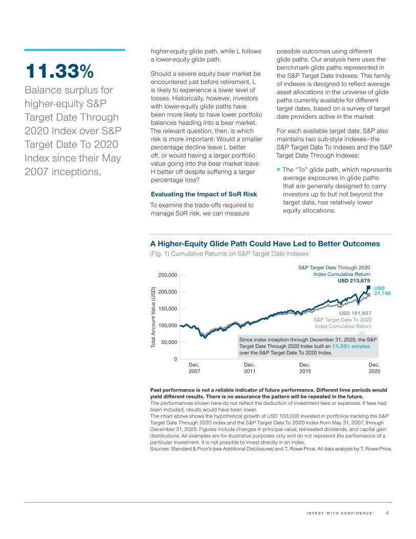
A Higher‑Equity Glide Path Could Have Led to Better Outcomes(Fig. 1) Cumulative Returns on S&P Target Date Indexes
Tota
l Acc
ount
Val
ue (U
SD) USD
21,748
0
50,000
100,000
150,000
200,000
250,000
Dec.2020
Dec.2015
Dec.2011
Dec.2007
Since index inception through December 31, 2020, the S&P Target Date Through 2020 Index built an 11.33% surplus over the S&P Target Date To 2020 Index.
S&P Target Date Through 2020Index Cumulative Return
USD 213,675
USD 191,927S&P Target Date To 2020Index Cumulative Return
Past performance is not a reliable indicator of future performance. Different time periods would yield different results. There is no assurance the pattern will be repeated in the future.The performances shown here do not reflect the deduction of investment fees or expenses. If fees had been included, results would have been lower. The chart above shows the hypothetical growth of USD 100,000 invested in portfolios tracking the S&P Target Date Through 2020 Index and the S&P Target Date To 2020 Index from May 31, 2007, through December 31, 2020. Figures include changes in principal value, reinvested dividends, and capital gain distributions. All examples are for illustrative purposes only and do not represent the performance of a particular investment. It is not possible to invest directly in an index.Sources: Standard & Poor’s (see Additional Disclosures) and T. Rowe Price. All data analysis by T. Rowe Price.
11.33%Balance surplus for higher‑equity S&P Target Date Through 2020 Index over S&P Target Date To 2020 Index since their May 2007 inceptions.
higher‑equity glide path, while L follows a lower‑equity glide path.
Should a severe equity bear market be encountered just before retirement, L is likely to experience a lower level of losses. Historically, however, investors with lower‑equity glide paths have been more likely to have lower portfolio balances heading into a bear market. The relevant question, then, is which risk is more important: Would a smaller percentage decline leave L better off, or would having a larger portfolio value going into the bear market leave H better off despite suffering a larger percentage loss?
Evaluating the Impact of SoR Risk
To examine the trade‑offs required to manage SoR risk, we can measure
possible outcomes using different glide paths. Our analysis here uses the benchmark glide paths represented in the S&P Target Date Indexes. This family of indexes is designed to reflect average asset allocations in the universe of glide paths currently available for different target dates, based on a survey of target date providers active in the market.
For each available target date, S&P also maintains two sub‑style indexes―the S&P Target Date To Indexes and the S&P Target Date Through Indexes:
■ The “To” glide path, which represents average exposures in glide paths that are generally designed to carry investors up to but not beyond the target date, has relatively lower equity allocations.
5
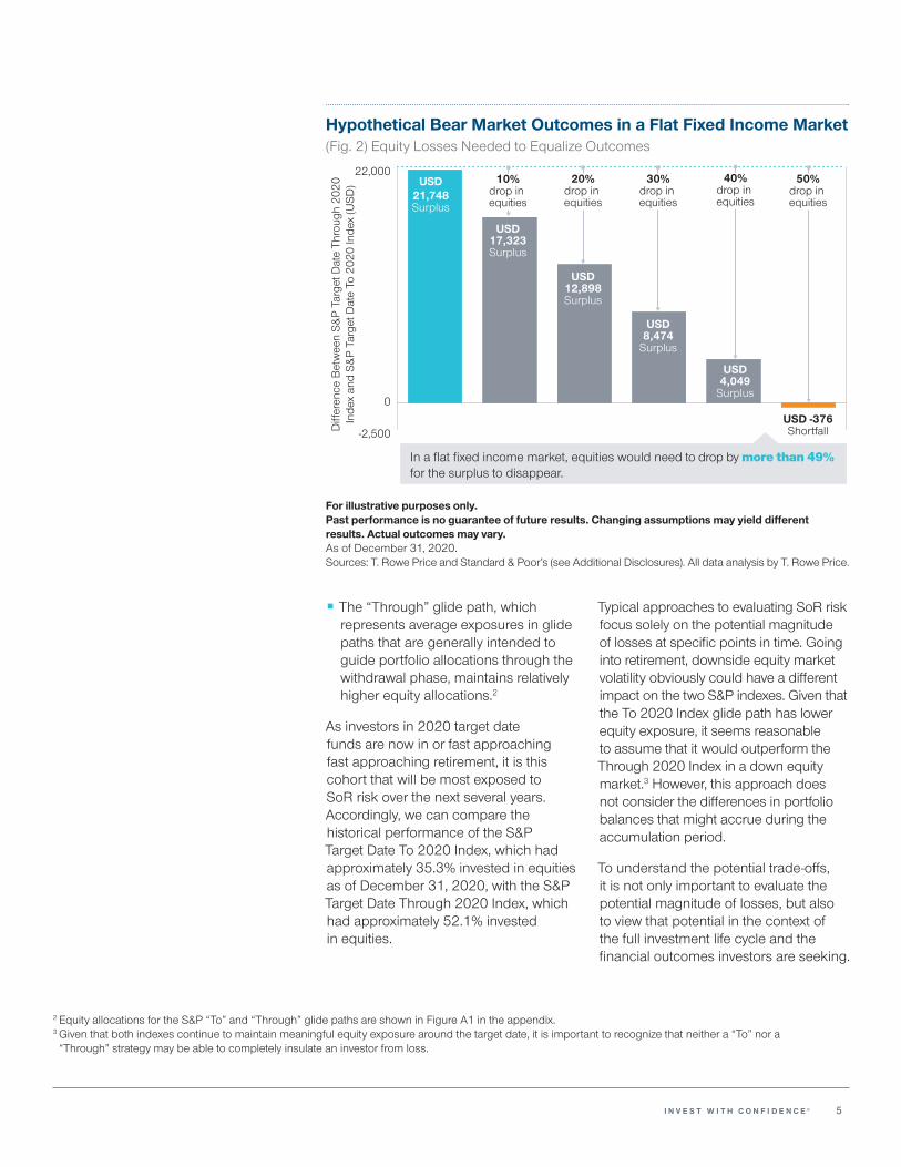
Hypothetical Bear Market Outcomes in a Flat Fixed Income Market(Fig. 2) Equity Losses Needed to Equalize Outcomes
-2,500
22,000
Diff
eren
ce B
etw
een
S&P
Targ
et D
ate
Thro
ugh
2020
In
dex
and
S&P
Targ
et D
ate
To 2
020
Inde
x (U
SD)
In a flat fixed income market, equities would need to drop by more than 49% for the surplus to disappear.
USD12,898Surplus
USD8,474
Surplus
USD -376Shortfall
10%drop in equities
20%drop in equities
30%drop in equities
40%drop in equities
50%drop in equities
0
USD21,748Surplus
USD17,323Surplus
USD4,049
Surplus
For illustrative purposes only. Past performance is no guarantee of future results. Changing assumptions may yield different results. Actual outcomes may vary. As of December 31, 2020.Sources: T. Rowe Price and Standard & Poor’s (see Additional Disclosures). All data analysis by T. Rowe Price.
2 Equity allocations for the S&P “To” and “Through” glide paths are shown in Figure A1 in the appendix. 3 Given that both indexes continue to maintain meaningful equity exposure around the target date, it is important to recognize that neither a “To” nor a “Through” strategy may be able to completely insulate an investor from loss.
■ The “Through” glide path, which represents average exposures in glide paths that are generally intended to guide portfolio allocations through the withdrawal phase, maintains relatively higher equity allocations.2
As investors in 2020 target date funds are now in or fast approaching fast approaching retirement, it is this cohort that will be most exposed to SoR risk over the next several years. Accordingly, we can compare the historical performance of the S&P Target Date To 2020 Index, which had approximately 35.3% invested in equities as of December 31, 2020, with the S&P Target Date Through 2020 Index, which had approximately 52.1% invested in equities.
Typical approaches to evaluating SoR risk focus solely on the potential magnitude of losses at specific points in time. Going into retirement, downside equity market volatility obviously could have a different impact on the two S&P indexes. Given that the To 2020 Index glide path has lower equity exposure, it seems reasonable to assume that it would outperform the Through 2020 Index in a down equity market.3 However, this approach does not consider the differences in portfolio balances that might accrue during the accumulation period.
To understand the potential trade‑offs, it is not only important to evaluate the potential magnitude of losses, but also to view that potential in the context of the full investment life cycle and the financial outcomes investors are seeking.
6
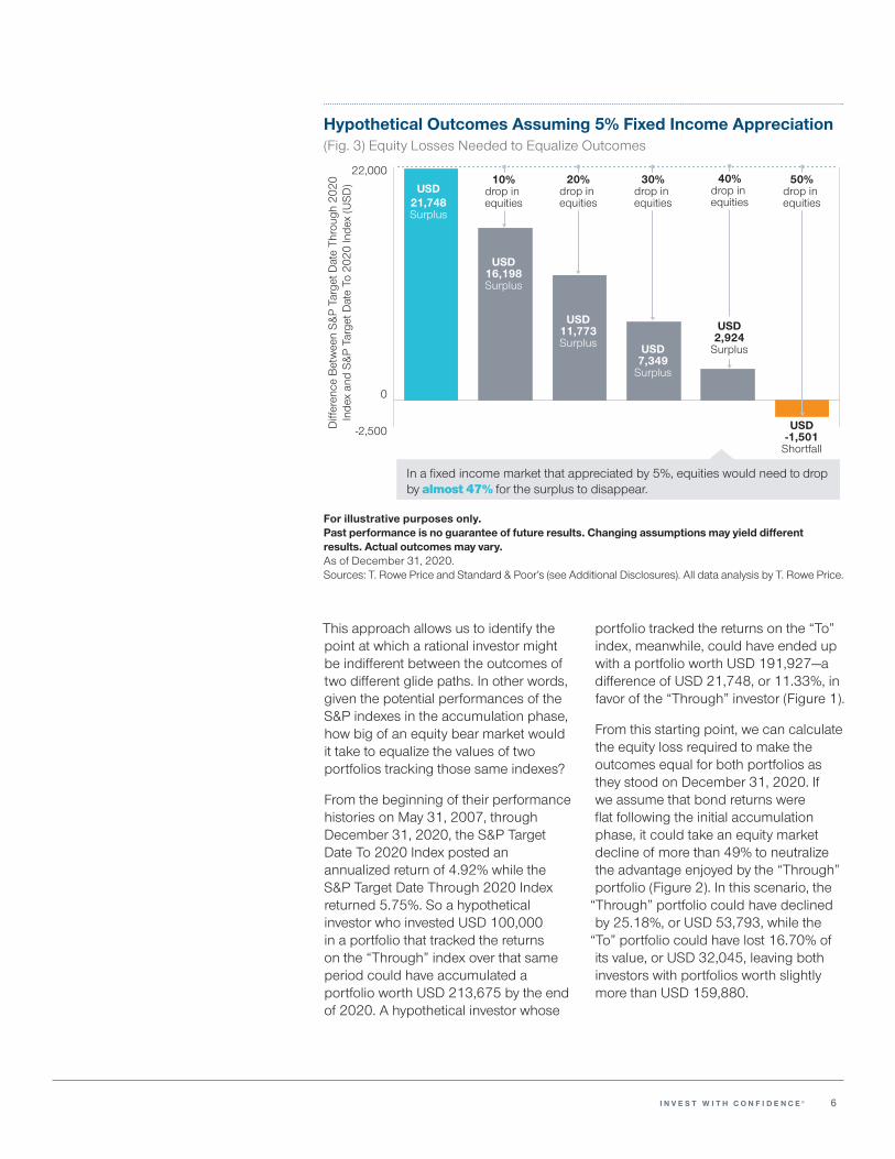
Hypothetical Outcomes Assuming 5% Fixed Income Appreciation(Fig. 3) Equity Losses Needed to Equalize Outcomes
-2,500
22,000
Diff
eren
ce B
etw
een
S&P
Targ
et D
ate
Thro
ugh
2020
In
dex
and
S&P
Targ
et D
ate
To 2
020
Inde
x (U
SD)
In a fixed income market that appreciated by 5%, equities would need to drop by almost 47% for the surplus to disappear.
USD11,773Surplus
USD-1,501
Shortfall
10%drop in equities
20%drop in equities
30%drop in equities
40%drop in equities
50%drop in equities
0
USD21,748Surplus
USD16,198Surplus
USD7,349
Surplus
USD2,924
Surplus
For illustrative purposes only. Past performance is no guarantee of future results. Changing assumptions may yield different results. Actual outcomes may vary. As of December 31, 2020.Sources: T. Rowe Price and Standard & Poor’s (see Additional Disclosures). All data analysis by T. Rowe Price.
This approach allows us to identify the point at which a rational investor might be indifferent between the outcomes of two different glide paths. In other words, given the potential performances of the S&P indexes in the accumulation phase, how big of an equity bear market would it take to equalize the values of two portfolios tracking those same indexes?
From the beginning of their performance histories on May 31, 2007, through December 31, 2020, the S&P Target Date To 2020 Index posted an annualized return of 4.92% while the S&P Target Date Through 2020 Index returned 5.75%. So a hypothetical investor who invested USD 100,000 in a portfolio that tracked the returns on the “Through” index over that same period could have accumulated a portfolio worth USD 213,675 by the end of 2020. A hypothetical investor whose
portfolio tracked the returns on the “To” index, meanwhile, could have ended up with a portfolio worth USD 191,927―a difference of USD 21,748, or 11.33%, in favor of the “Through” investor (Figure 1).
From this starting point, we can calculate the equity loss required to make the outcomes equal for both portfolios as they stood on December 31, 2020. If we assume that bond returns were flat following the initial accumulation phase, it could take an equity market decline of more than 49% to neutralize the advantage enjoyed by the “Through” portfolio (Figure 2). In this scenario, the
“Through” portfolio could have declined by 25.18%, or USD 53,793, while the
“To” portfolio could have lost 16.70% of its value, or USD 32,045, leaving both investors with portfolios worth slightly more than USD 159,880.
7
4 For additional details on the methodology used in our analysis, please see the appendix.
Even in an environment where bond allocations generated a 5% cumulative return during the bear market period, equity prices still might have to fall almost 47% to produce the same ending values for the two portfolios (Figure 3).
In this analysis, we focus on portfolio balances because, as a simplifying assumption, the current balance can be viewed as the present value of future retirement spending. If we assume that an individual has a set spending strategy, then, all else being equal, a higher balance potentially means that he or she could spend the same amount over a longer period (i.e., the stream of income would last longer) or spend more over a shorter horizon.
In both cases, the SoR risk resulting from market volatility near retirement could have a significant impact on retirement income. However, unless the equity decline were even larger than in the hypothetical scenarios outlined above, the more conservative
“To” investor would not enjoy a withdrawal advantage over the more growth‑oriented “Through” investor.
From an outcome‑oriented perspective, the benefit of capturing the equity risk premium over a long investment horizon potentially would outweigh the impact of SoR risk.
SoR Risk Over the Longer Run
To put these potential trade‑offs in a broader perspective, it is helpful to observe similar scenarios across a wider range of potential market conditions. Unfortunately, the S&P Target Date To and Through Indexes have relatively short track records, only dating back to May 2007. However, we can calculate a longer‑term return comparison by taking the S&P “To” and “Through” glide path allocations and plugging in longer‑term historical stock and bond returns.
To do this, we calculated the performances of hypothetical portfolios tracking the S&P
“To” and “Through” glide paths based on actual historical stock and bond returns over the past 95 years.4 Our proxy for equity returns was the S&P 500 Index, as calculated by Ibbotson Associates, a financial research firm. Bond returns were based on the Ibbotson U.S. Investment Grade Bond Series.
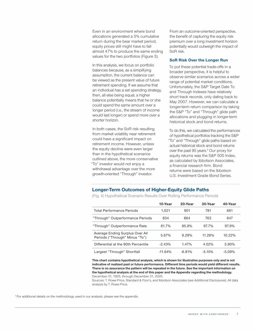
Longer‑Term Outcomes of Higher‑Equity Glide Paths(Fig. 4) Hypothetical Scenario Results Over Rolling Performance Periods
10‑Year 20‑Year 30‑Year 40‑Year
Total Performance Periods 1,021 901 781 661
“Through” Outperformance Periods 834 864 763 647
“Through” Outperformance Rate 81.7% 95.9% 97.7% 97.9%
Average Ending Surplus Over All Periods (“Through” Minus “To”) 5.67% 9.29% 11.26% 10.22%
Differential at the 90th Percentile ‑2.43% 1.47% 4.02% 3.90%
Largest “Through” Shortfall ‑11.64% ‑6.81% ‑5.15% ‑5.09%
This chart contains hypothetical analysis, which is shown for illustrative purposes only and is not indicative of realized past or future performance. Different time periods would yield different results. There is no assurance the pattern will be repeated in the future. See the important information on the hypothetical analysis at the end of this paper and the Appendix regarding the methodology.December 31, 1925, through December 31, 2020.Sources: T. Rowe Price, Standard & Poor’s, and Ibbotson Associates (see Additional Disclosures). All data analysis by T. Rowe Price.
8
This allowed us to extend our analysis back to 1925—the inception date for the Ibbotson return series.
To reflect the varying situations of target date investors―some of whom may have defaulted into their current glide paths as the result of mid career job changes―we calculated portfolio performance over 10‑, 20‑, 30‑, and 40‑year time horizons, with each horizon ending at the retirement point of the glide path. For each time horizon, we specified a starting salary, a starting portfolio balance, an assumed rate of salary growth, and an assumed annual contribution level. These assumptions are shown in Figure A2 in the appendix.
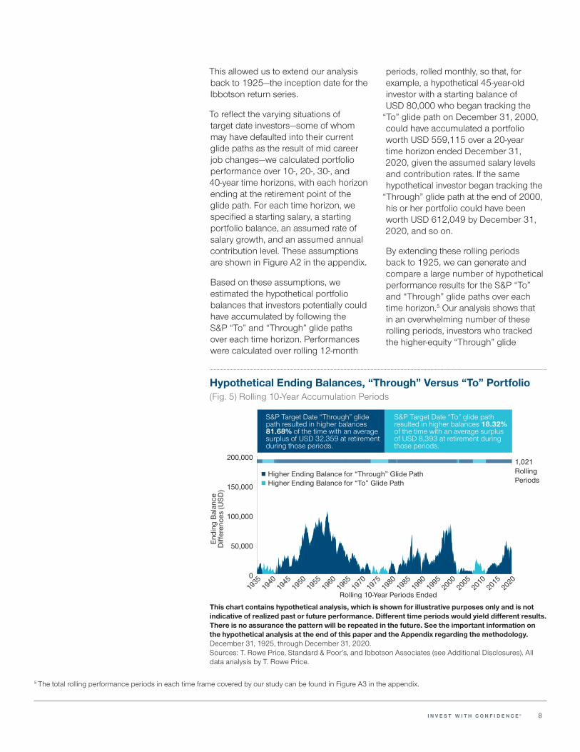
Based on these assumptions, we estimated the hypothetical portfolio balances that investors potentially could have accumulated by following the S&P “To” and “Through” glide paths over each time horizon. Performances were calculated over rolling 12‑month
periods, rolled monthly, so that, for example, a hypothetical 45‑year‑old investor with a starting balance of USD 80,000 who began tracking the
“To” glide path on December 31, 2000, could have accumulated a portfolio worth USD 559,115 over a 20‑year time horizon ended December 31, 2020, given the assumed salary levels and contribution rates. If the same hypothetical investor began tracking the
“Through” glide path at the end of 2000, his or her portfolio could have been worth USD 612,049 by December 31, 2020, and so on.
By extending these rolling periods back to 1925, we can generate and compare a large number of hypothetical performance results for the S&P “To” and “Through” glide paths over each time horizon.5 Our analysis shows that in an overwhelming number of these rolling periods, investors who tracked the higher‑equity “Through” glide
5 The total rolling performance periods in each time frame covered by our study can be found in Figure A3 in the appendix.
Hypothetical Ending Balances, “Through” Versus “To” Portfolio(Fig. 5) Rolling 10‑Year Accumulation Periods
1,021RollingPeriods
Rolling 10-Year Periods Ended
Endi
ng B
alan
ceD
iffer
ence
s (U
SD)
Higher Ending Balance for “To” Glide PathHigher Ending Balance for “Through” Glide Path
0
50,000
100,000
150,000
200,000
20202015
20102005
20001995
19901985
19801975
19701965
19601955
19501945
19401935
S&P Target Date “Through” glide path resulted in higher balances 81.68% of the time with an average surplus of USD 32,359 at retirement during those periods.
S&P Target Date “To” glide path resulted in higher balances 18.32% of the time with an average surplus of USD 8,393 at retirement during those periods.
0
1
202020152010200520001995199019851980197519701965196019551950194519401935
This chart contains hypothetical analysis, which is shown for illustrative purposes only and is not indicative of realized past or future performance. Different time periods would yield different results. There is no assurance the pattern will be repeated in the future. See the important information on the hypothetical analysis at the end of this paper and the Appendix regarding the methodology.December 31, 1925, through December 31, 2020.Sources: T. Rowe Price, Standard & Poor’s, and Ibbotson Associates (see Additional Disclosures). All data analysis by T. Rowe Price.
9
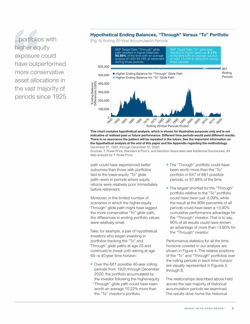
Hypothetical Ending Balances, “Through” Versus “To” Portfolio(Fig. 6) Rolling 20‑Year Accumulation Periods
901RollingPeriods
Rolling 20-Year Periods Ended
Endi
ng B
alan
ceD
iffer
ence
s (U
SD)
Higher Ending Balance for “To” Glide PathHigher Ending Balance for “Through” Glide Path
0
100,000
200,000
300,000
400,000
500,000
600,000
20202015
20102005
20001995
19901985
19801975
19701965
19601955
19501945
S&P Target Date “Through” glide path resulted in higher balances 95.89% of the time with an average surplus of USD 93,785 at retirement during those periods.
S&P Target Date “To” glide pathresulted in higher balances 4.11% of the time with an average surplus of USD 13,149 at retirement during those periods.
0
1
2020201520102005200019951990198519801975197019651960195519501945
This chart contains hypothetical analysis, which is shown for illustrative purposes only and is not indicative of realized past or future performance. Different time periods would yield different results. There is no assurance the pattern will be repeated in the future. See the important information on the hypothetical analysis at the end of this paper and the Appendix regarding the methodology.December 31, 1925, through December 31, 2020.Sources: T. Rowe Price, Standard & Poor’s, and Ibbotson Associates (see Additional Disclosures). All data analysis by T. Rowe Price.
path could have experienced better outcomes than those with portfolios tied to the lower‑equity “To” glide path―even in periods where equity returns were relatively poor immediately before retirement.
Moreover, in the limited number of scenarios in which the higher‑equity
“Through” glide path might have lagged the more conservative “To” glide path, the differences in ending portfolio values were relatively small.
Take, for example, a pair of hypothetical investors who began investing in portfolios tracking the “To” and
“Through” glide paths at age 25 and continued to invest until retiring at age 65―a 40‑year time horizon:
■ Over the 661 possible 40‑year rolling periods from 1925 through December 2020, the portfolio accumulated by the investor following the higher‑equity
“Through” glide path could have been worth an average 10.22% more than the “To” investor’s portfolio.
■ The “Through” portfolio could have been worth more than the “To” portfolio in 647 of 661 possible periods, or 97.88% of the time.
■ The largest shortfall for the “Through” portfolio relative to the “To” portfolio could have been just ‑5.09%, while the result at the 90th percentile of all periods could have been a +3.90% cumulative performance advantage for the “Through” investor. That is to say, 90% of all results could have shown an advantage of more than +3.90% for the “Through” investor.
Performance statistics for all the time horizons covered in our analysis are shown in Figure 4. The relative positions of the “To” and “Through” portfolios over the rolling periods in each time horizon are visually represented in Figures 5 through 8.
The relationships described above held across the vast majority of historical accumulation periods we examined. The results drive home the historical
...portfolios with higher equity exposure could have outperformed more conservative asset allocations in the vast majority of periods since 1925.
10
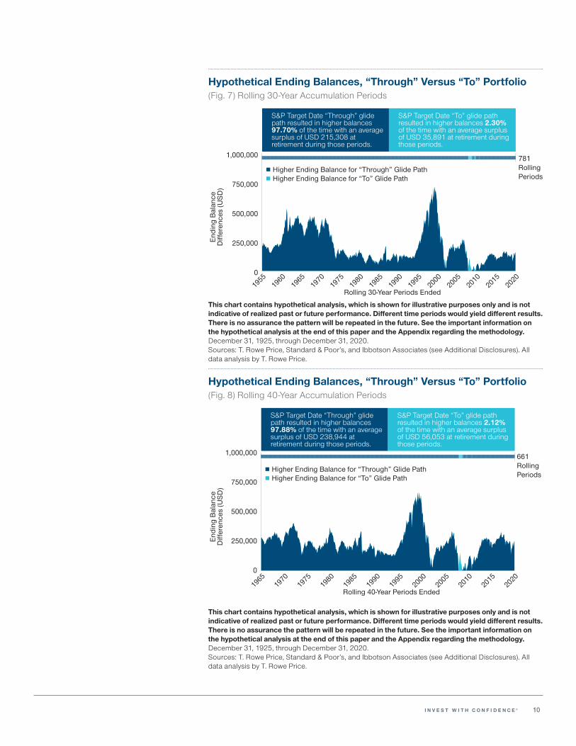
Hypothetical Ending Balances, “Through” Versus “To” Portfolio(Fig. 8) Rolling 40‑Year Accumulation Periods
Rolling 40-Year Periods Ended
Endi
ng B
alan
ceD
iffer
ence
s (U
SD)
Higher Ending Balance for “To” Glide PathHigher Ending Balance for “Through” Glide Path
0
250,000
500,000
750,000
1,000,000
20202015
20102005
20001995
19901985
19801975
19701965
S&P Target Date “Through” glide path resulted in higher balances 97.88% of the time with an average surplus of USD 238,944 at retirement during those periods.
S&P Target Date “To” glide path resulted in higher balances 2.12% of the time with an average surplus of USD 56,053 at retirement during those periods.
661RollingPeriods
0202020152010200520001995199019851980197519701965
This chart contains hypothetical analysis, which is shown for illustrative purposes only and is not indicative of realized past or future performance. Different time periods would yield different results. There is no assurance the pattern will be repeated in the future. See the important information on the hypothetical analysis at the end of this paper and the Appendix regarding the methodology.December 31, 1925, through December 31, 2020.Sources: T. Rowe Price, Standard & Poor’s, and Ibbotson Associates (see Additional Disclosures). All data analysis by T. Rowe Price.
Hypothetical Ending Balances, “Through” Versus “To” Portfolio(Fig. 7) Rolling 30‑Year Accumulation Periods
781RollingPeriods
Rolling 30-Year Periods Ended
Endi
ng B
alan
ceD
iffer
ence
s (U
SD)
Higher Ending Balance for “To” Glide PathHigher Ending Balance for “Through” Glide Path
0
250,000
500,000
750,000
1,000,000
20202015
20102005
20001995
19901985
19801975
19701965
19601955
S&P Target Date “Through” glide path resulted in higher balances 97.70% of the time with an average surplus of USD 215,308 at retirement during those periods.
S&P Target Date “To” glide pathresulted in higher balances 2.30% of the time with an average surplus of USD 35,891 at retirement during those periods.
020202015201020052000199519901985198019751970196519601955
This chart contains hypothetical analysis, which is shown for illustrative purposes only and is not indicative of realized past or future performance. Different time periods would yield different results. There is no assurance the pattern will be repeated in the future. See the important information on the hypothetical analysis at the end of this paper and the Appendix regarding the methodology.December 31, 1925, through December 31, 2020.Sources: T. Rowe Price, Standard & Poor’s, and Ibbotson Associates (see Additional Disclosures). All data analysis by T. Rowe Price.
11
reality that portfolios with higher equity exposure could have outperformed more conservative asset allocations in the vast majority of periods since 1925.
Even as the accumulation periods were shortened and the opportunity to capture the equity risk premium was narrowed, the hypothetical outcomes in our analysis continued to significantly favor higher‑equity glide paths. Even over an accumulation period as short as 10 years, a portfolio tracking the S&P “Through” glide path could have outperformed in 834 (or almost 82%) of 1,021 possible rolling 10‑year periods from 1925 through December 2020.
It is fair to recognize that equity bear markets can have a more substantial impact over shorter investment horizons. Indeed, the worst hypothetical result for the “Through” portfolio in our rolling 10‑year analysis was a ‑11.64% shortfall relative to the “To” portfolio. However, the average shortfall over those same periods could have been just ‑3.13%.
In our view, a difference of less than 12% in ending portfolio values is meaningful but hardly catastrophic as a worst‑case scenario. This is why we believe the potential benefits of a higher‑equity glide path more than outweigh potential SoR risks for most retirement investors.
Conclusions
As investors approach retirement, it is not surprising that they may become more sensitive to the risk of a short‑term market decline. However, a narrow focus on risk of loss does not take into account the full range of risks that retirement investors face. We believe it is important to evaluate SoR risk in a broader, more holistic context, especially if we consider longevity risk and the fact that investors will likely
need their income streams to last decades into retirement.
Most retirement investors primarily seek durable, sustainable income streams to support their retirement needs. For these investors, the benefits of a growth‑oriented glide path that enables them to accumulate larger portfolio balances during the accumulation phase will tend to meaningfully outweigh the impact of even a large market decline close to retirement, in our view. Efforts to mitigate SoR risk by shifting to a more conservative glide path historically have come at a price: lower expected returns, slower portfolio growth, lower account balances, and lower or less sustainable income streams throughout retirement.
This is not to say that the choice of a conservative glide path is always unjustified. Some investors, given their circumstances, may rationally prefer a strategy that limits the variability of account balances around retirement. But SoR risk mitigation in and of itself does not appear to be a particularly good motive and brings with it other risks. This highlights the need for investors to consider SoR risk within the context of their total financial situations―including their anticipated contribution levels and postretirement income needs.
For investors who have had the opportunity to accumulate savings over the course of long working careers, higher‑equity glide paths historically could have delivered higher retirement balances in the vast majority of long‑run periods, even after taking SoR risk into account. We believe investors would be wise to consider this experience when choosing target date strategies.
We believe it is important to evaluate SoR risk in a broader, more holistic context, especially if we consider longevity risk...

12
Important Information—Hypothetical Analysis
Where noted, the results shown above are hypothetical, do not reflect actual investment results, and are not indicative of future results. Hypothetical results were developed with the benefit of hindsight and have inherent limitations. Hypothetical results do not reflect actual trading or the effect of material economic and market factors on the decision‑making process. These results are derived from the actual returns of the indicated indices. Index results are for illustrative purposes only and are not indicative of any T. Rowe Price investment. Results do not reflect any fees or expenses. If fees had been included, results would have been lower. Investors cannot invest directly in an index.
Additional Disclosures
Copyright © 2021, S&P Global Market Intelligence (and its affiliates, as applicable). Reproduction of any information, data or material, including ratings (“Content”) in any form is prohibited except with the prior written permission of the relevant party. Such party, its affiliates and suppliers (“Content Providers”) do not guarantee the accuracy, adequacy, completeness, timeliness or availability of any Content and are not responsible for any errors or omissions (negligent or otherwise), regardless of the cause, or for the results obtained from the use of such Content. In no event shall Content Providers be liable for any damages, costs, expenses, legal fees, or losses (including lost income or lost profit and opportunity costs) in connection with any use of the Content. A reference to a particular investment or security, a rating or any observation concerning an investment that is part of the Content is not a recommendation to buy, sell or hold such investment or security, does not address the suitability of an investment or security and should not be relied on as investment advice. Credit ratings are statements of opinions and are not statements of fact.
©2021 Morningstar, Inc. All rights reserved. The information contained herein: (1) is proprietary to Morningstar and/or its content providers; (2) may not be copied or distributed; and (3) is not warranted to be accurate, complete, or timely. Neither Morningstar nor its content providers are responsible for any damages or losses arising from any use of this information. Past performance is no guarantee of future results.
13
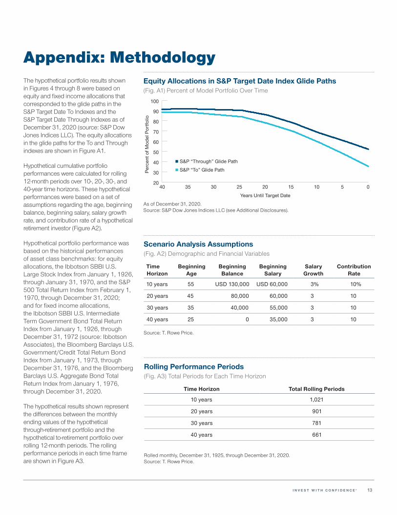
Appendix: MethodologyThe hypothetical portfolio results shown in Figures 4 through 8 were based on equity and fixed income allocations that corresponded to the glide paths in the S&P Target Date To Indexes and the S&P Target Date Through Indexes as of December 31, 2020 (source: S&P Dow Jones Indices LLC). The equity allocations in the glide paths for the To and Through indexes are shown in Figure A1.
Hypothetical cumulative portfolio performances were calculated for rolling 12‑month periods over 10‑, 20‑, 30‑, and 40‑year time horizons. These hypothetical performances were based on a set of assumptions regarding the age, beginning balance, beginning salary, salary growth rate, and contribution rate of a hypothetical retirement investor (Figure A2).
Hypothetical portfolio performance was based on the historical performances of asset class benchmarks: for equity allocations, the Ibbotson SBBI U.S. Large Stock Index from January 1, 1926, through January 31, 1970, and the S&P 500 Total Return Index from February 1, 1970, through December 31, 2020; and for fixed income allocations, the Ibbotson SBBI U.S. Intermediate Term Government Bond Total Return Index from January 1, 1926, through December 31, 1972 (source: Ibbotson Associates), the Bloomberg Barclays U.S. Government/Credit Total Return Bond Index from January 1, 1973, through December 31, 1976, and the Bloomberg Barclays U.S. Aggregate Bond Total Return Index from January 1, 1976, through December 31, 2020.
The hypothetical results shown represent the differences between the monthly ending values of the hypothetical through‑retirement portfolio and the hypothetical to‑retirement portfolio over rolling 12‑month periods. The rolling performance periods in each time frame are shown in Figure A3.
Equity Allocations in S&P Target Date Index Glide Paths(Fig. A1) Percent of Model Portfolio Over Time
Years Until Target Date
Perc
ent o
f Mod
el P
ortfo
lio
20
30
40
50
60
70
80
90
100
0510152025303540
S&P “To” Glide Path
S&P “Through” Glide Path
As of December 31, 2020.Source: S&P Dow Jones Indices LLC (see Additional Disclosures).
Scenario Analysis Assumptions(Fig. A2) Demographic and Financial Variables
Time Horizon
Beginning Age
Beginning Balance
Beginning Salary
Salary Growth
Contribution Rate
10 years 55 USD 130,000 USD 60,000 3% 10%
20 years 45 80,000 60,000 3 10
30 years 35 40,000 55,000 3 10
40 years 25 0 35,000 3 10
Source: T. Rowe Price.
Rolling Performance Periods(Fig. A3) Total Periods for Each Time Horizon
Time Horizon Total Rolling Periods
10 years 1,021
20 years 901
30 years 781
40 years 661
Rolled monthly, December 31, 1925, through December 31, 2020.Source: T. Rowe Price.
14
Important Information
This material is provided for informational purposes only and is not intended to be investment advice or a recommendation to take any particular investment action.
The views contained herein are those of the authors as of April 2021 and are subject to change without notice; these views may differ from those of other T. Rowe Price associates.
This information is not intended to reflect a current or past recommendation, investment advice of any kind, or a solicitation of an offer to buy or sell any securities or investment services. The opinions and commentary provided do not take into account the investment objectives or financial situation of any particular investor or class of investor. Investors will need to consider their own circumstances before making an investment decision.
Information contained herein is based upon sources we consider to be reliable; we do not, however, guarantee its accuracy.
Past performance is not a reliable indicator of future performance. All investments are subject to market risk, including the possible loss of principal. The principal value of target date strategies is not guaranteed at any time, including at or after the target date, which is the approximate date when investors plan to retire. A substantial allocation to equities both prior to and after the target date can result in greater volatility over short term horizons. All charts and tables are shown for illustrative purposes only.
T. Rowe Price Investment Services, Inc.
© 2021 T. Rowe Price. All rights reserved. T. ROWE PRICE, INVEST WITH CONFIDENCE, and the bighorn sheep design are, collectively and/or apart, trademarks
ID0004078 (04/2021)202103‑1548079
T. Rowe Price focuses on delivering investment management excellence that investors can rely on—now and over the long term.
To learn more, please visit troweprice.com.