A deterministic algorithm for the three-dimensionaldiameter problemCitation for published version (APA):Matousek, J., & Cheong, O. (1992). A deterministic algorithm for the three-dimensional diameter problem.(Universiteit Utrecht. UU-CS, Department of Computer Science; Vol. 9245). Utrecht: Utrecht University.

Document status and date:Published: 01/01/1992

Document Version:Publisher’s PDF, also known as Version of Record (includes final page, issue and volume numbers)

Please check the document version of this publication:

• A submitted manuscript is the version of the article upon submission and before peer-review. There can beimportant differences between the submitted version and the official published version of record. Peopleinterested in the research are advised to contact the author for the final version of the publication, or visit theDOI to the publisher's website.• The final author version and the galley proof are versions of the publication after peer review.• The final published version features the final layout of the paper including the volume, issue and pagenumbers.Link to publication

General rightsCopyright and moral rights for the publications made accessible in the public portal are retained by the authors and/or other copyright ownersand it is a condition of accessing publications that users recognise and abide by the legal requirements associated with these rights.

• Users may download and print one copy of any publication from the public portal for the purpose of private study or research. • You may not further distribute the material or use it for any profit-making activity or commercial gain • You may freely distribute the URL identifying the publication in the public portal.

If the publication is distributed under the terms of Article 25fa of the Dutch Copyright Act, indicated by the “Taverne” license above, pleasefollow below link for the End User Agreement:

www.tue.nl/taverne

Take down policyIf you believe that this document breaches copyright please contact us at:

openaccess@tue.nl

providing details and we will investigate your claim.

Download date: 18. Mar. 2019

A Deterministic Algorithm for the Three-Dimensional Diameter Problem

Jifi Matousek Otfried Schwarzkopf

RUU-CS-92-45 December 1992

Utrecht University Department of Computer Science

Padualaan 14, P.O. Box 80.089,

3508 TB Utrecht, The Netherlands,

Tel. : + 31 - 30 - 531454

A Deterministic Algorithm for the Three-Dimensional Diameter Problem

Jifi Matousek Otfried Schwarzkopf

Technical Report RUU-CS-92-45 December 1992

Department of Computer Science Utrecht University

P.O.Box 80.089 3508 TB Utrecht The Netherlands

~ ...... . )

A Deterministic Algorithm for the Three-Dimensional Diameter Problem*

Jifi Matousek Otfried Schwarzkopf

Abstract

We give a deterministic algorithm for computing the diameter of an n point set in three dimensions with O(nlogC n) running time, c a constant. Keywords: Computational geometry, diameter, three-dimensional, parametric search, deterministic algorithm, £-approximation.

1 Introduction

We consider the following problem: Given an n-point set P in three-dimensional space, compute its diameter diam(P), defined as the maximum distance between a pair of points in P. This problem was solved by Clarkson and Shor [CS89] by a randomized algorithm with optimal expected running time 0 (n log n). However, it seems quite difficult to con­struct a deterministic algorithm with a comparable asymptotic efficiency.

Chuelle et al. [CEGS92] applied Megiddo's parametric search [Meg83] in connection with the Clarkson-Shor algorithm and further techniques and obtained a deterministic O(nl+t) algorithm, where £ > 0 is an arbitrarily small constant. In this paper, we improve this running time to 0 (n polylog n) (we use polylog n as a generic notation for a function of the form (log n)C , c > 0 a constant).

Our basic approach is the same as that of [CEGS92]. Also the basic scheme for achieving the improvement has appeared in previous works: While Chazelle et al. divide the problem into a constant number of subproblems, we refine the "divide" step and use a larger number of subproblems (nit for a small but positive constant LX). With this change, some computations which are trivially done for a constant number of subproblems become more demanding.

In order to apply parametric search in this situation, it is helpful to change the usual approach to parametric search. In many presentations and applications of the parametric search technique, the need for designing a parallel algorithm is emphasized. What is really required, however, is a sequential algorithm, only with comparisons involving the value of the unknown parameter collected into "batches" of independent comparisons. This has already been pointed out by various authors, and we consider it an important part of the parametric search method, which is very easy to overlook. It is this slight shift of attention which enables us to solve problems which we could not overcome before .

• This research was supported by the Netherlands' Organization for Scientific Research (NWO) and partially by the ESP~T Basic Research Action No. 7141 (project ALCOM I). J. M. acknowledges support by Humboldt Research Fellowship. Part of this research was done while he visited Utrecht University.

1

Theorem 1 Given a set P of n points in tbree-dimensional space, tbe diameter of P can be determined by a deterministic algoritbm in time O(npolylog n).

The algorithm is too complicated and has too large constants hidden in the asymptotic notation to be of any practical value; it is only a theoretical contribution to the problem of deterministic asymptotic complexity of the diameter problem. And, one must ask, are all these heavy tools really necessary, or are we just blinded by the various techniques available to overlook a simple elementary solution?

2 Diameter and Parametric Search

Let P be a given set of n points in 3-space. A quadratic algorithm for computing diam(P) is trivial. Using randomization, Clarkson and Shor [CS89] have obtained an algorithm whose expected running time (over the internal randomizations that it performs) is O(nlogn). They :first transform the problem to the following ball problem:

Given n unit-balls and n points in 3-space, determine whether any point lies outside the common intersection of the balls.

This problem is then solved using a randomized incremental algorithm. In their algo­rithm, both the transformation to the ball problem, and the solution of the latter involve randomization.

Chazelle et al. [CEGS92] considered the problem of making this algorithm determin­istic. Fortunately, the transformation to the ball problem can be made deterministic by applying Megiddo's parametric search [Meg83]. Unfortunately, this transformation adds some additional requirement on the solution of the ball problem, and Chazelle et al. [CEGS92] could only give a deterministic solution to the latter with running time O(nl+t), for an arbitrarily small e > O. As stated in the introduction, we will be able to get closer to the complexity of the randomized algorithm. Matching the randomized complexity remains as a challenge for future research.

Let us start by describing the application of parametric search (see e.g., Megiddo's original work [Meg83] or the paper of Chazelle et al. [CEGS92] for a more detailed explanation of the parametric search paradigm): We assume that we are given an algorithm A that solves the following "fixed-size" problem: Given n points P, and a parameter 5 > 0, determine whether diam(P) is less than, equal to, or greater than 5. (Observe that this is a restricted version of the ball problem mentioned above, since we have to determine whether any point in P lies outside the intersection of the balls of radius 5 around the points in P).

The algorithm A plays a dual role in the overall algorithm for diameter computa­tion. First, it serves as a oracle which, given a specific value 5* of 5, decides whether 5* < diam(P}, 5* = diam(P) or 5* > diam(P). Second, it serves as so-called generic algorithm (let us remark that in general, these roles can be played by different algorithms in parametric search applications, but for us it is suitable to use A in both roles). For this second role, we require that A uses the information about the parameter 5 in a restricted manner. That is, we assume that 5 is not explicitly available to A, but rather that A has access to an oracle that allows it to test whether 5 is less than or equal to some value 5* > O. Note that this allows the algorithm A to test the sign of arbitrary polynomials

2

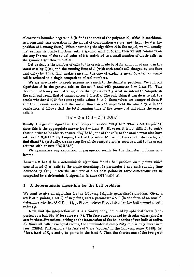
of constant-bounded degree in 0 (it finds the roots of the polynomial, which is considered as a constant-time operation in the model of computation we use, and then it locates the position of 0 among them). When describing the algorithm A in the sequel, we will usually first explain its oracle function, with a specific value of 0, and then we will comment on the way the use of the actual value of 0 is restricted to a small number of oracle calls, in the generic algorithm role of A.

Let us denote the number of calls to the oracle made by A for an input of size n in the worst case by Q (n), and the running time of A (with each oracle call charged by one time unit only) by T(n). This makes sense for the case of explicitly given 0, when an oracle call is reduced to a single comparison of real numbers.

We are now ready to apply parametric search to the diameter problem. We run our algorithm A in the generic role on the set P and with parameter 0 = diam(P). This definition of 0 may seem strange, since diam(P) is exactly what we intend to compute in the end, but recall that A cannot access 0 directly. The only thing it can do is to ask the oracle whether 0 ~ 0* for some specific values l)* > OJ these values are computed from P and the previous answers of the oracle. Since we can implement the oracle by A in the oracle role, it follows that the total running time of the generic A including the oracle calls is

T(n) + Q(n)T(n) = O(T(n)Q(n)).

Finally, the generic algorithm A will stop and answer "EQUAL". This is not surprising, since this is the appropriate answer for 0 = diam(P). However, it is not difficult to verify that in order to be able to answer "EQUAL", one of the calls to the oracle must also have returned "EQUAL". By keeping track of the values 0* used in the calls to the oracle, we find diam(P}. (Actually, we can stop the whole computation as soon as a call to the oracle returns with answer "EQUAL").

We summarize our exposition of parametric search for the diameter problem in a lemma.

Lemma Z Let A be a deterministic algorithm for the ball problem on n points which uses at most Q(n) calls to the oracle describing the parameter 0 and with running time bounded by T(n). Then the diameter of a set of n points in three dimensions can be computed by a deterministic algorithm in time O(T(n)Q(n)).

3 A deterministic algorithm for the ball problem

We want to give an algorithm for the following (slightly generalized) problem: Given a set P of n points, a set Q of m points, and a parameter 0 > 0 (in the form of an oracle), determine whether Q c K := n"EP B(p, 0), where B(p, p) denotes the ball around l' with radius p.

Note that the intersection set K is a convex body, bounded by spherical facets (sup­ported by a ball B(p, 0) for some l' E P). The facets are bounded by circular edges (circular arcs in three dimensions, arising as the intersection of the boundaries of two balls of radius l)). Since all balls have equal radius, the combinatorial complexity of K is only linear in n (see [CS89]). Furthermore, the facets of K are "convex" in the following sense [CS89]: Let f be a facet of K, x and 'Y be points in the facet f. Then the shorter one of the two great

3

circle arcs connecting x and y lies completely in f (note that x and y cannot be antipodes of each other, unless there is only one ball).

Clarkson and Shor's randomized algorithm [CS89] works as follows: It computes the body K by a randomized incremental construction, picks some point 0 in the interior of K, and centrally projects the edges of K from 0 on a unit-sphere around o. This results in a planar map for which a planar point location structure is constructed. It then locates every point of Q using this structure. On the top level of the algorithm, one has P = Qj the above generalized version of the ball problem will be a typical subproblem appearing in a recursion in our algorithm.

The part which appears difficult to do deterministically is the construction of K. In­stead of an incremental construction, we will use a divide-and-conquer approach. It will also be convenient to combine the recursive construction of K with the location of the points of Q in K.

In the first step, we will identify a subset R of P. We will compute KR := npER B(p, 5). The surface of KR consists of vertices, edges (circular arcs) and facets (portions of unit spheres bounded by circular arcs). The total number of these features is O(lRI). We form a decomposition 'J(R) of KR into O(lRI) cells, each cell cr E 'J(R) being described by a constant number of real parameters. We call these cells (for a lack of a better name) bricks. A natural way to produce such a decomposition would be as follows: for every facet f of KR, choose a point Vf E f, and subdivide f into "spherical triangles" by connecting Vf to the vertices of f by great circle arcs. Then choose a point 0 in the interior of KR and for every spherical triangle 'T on the surface of KR, connect each its point with 0 by a segment, forming a brick ("spherical tetrahedron") corresponding to 'T.

This is essentially the way which is used (and works) in Chazelle et al's method [CEGS92] (although their definition contains some formal imprecisions). It turns out, however, that this decomposition method is not good enough for our purposes, and we have to choose another one, analogous to vertical decomposition in the plane. The precise definition will be given in Section 4, for time being we suppose that we have the subdivision 'J(R) of KR into OURI) bricks, of some kind.

For every brick cr E 'J(R) we compute the set Qa of points in Q lying in cr, and also the set P a of pEP such that cr is not completely contained in B (p, 5). If any point of Q turns out to lie outside KR, we are done. Otherwise, we proceed by solving the subproblems defined by the sets P a, Q a and by 5 for every cr E 'J ( R). When the cardinality of either PO' or QO' drops below some constant, we solve the problem naively.

Thus, we obtain the following recursion for the time T(n, m) necessary to solve the ball problem.

T(n, m) = S(n) + S'(n, m) + L T(na, mal. aE'J"(R)

Here, S(n) is the time necessary to identify a proper subset R, triangulate it and identify the subsets P a for all cr E 'J(R). S'(n, m) is the time necessary to identify the subsets Qaj and na and ma are the cardinalities of Pa and Qa, resp. Note that LaE'J"(R) m.,. = m.

Let r > 1 be a parameter bounded by a constant. Using e-net theory and results from [Mat91a], it is possible to find, in time S(n) = O(nlogr), a subset ReP of size O(rlogr) with the property that na ~ n/r for every cr E 'J(R). With these values and S'(n,m) = O(m), the above recurrence solves to O(mlogn+nl+t), for a constant e > 0

4

which can be made arbitrarily small by increasing r. This is essentially the solution by Chazelle et al. [CEGS92].

To get rid ofthe polynomial factor O(n£), however, we want to find a suitable subset R of larger size, as in the following lemma.

Lemma 3 Tbere exists a positive constant (x, sucb tbat for an n point set P in tbree dimensions, and a parameter [j > 0 given as an oracle, we can identify in time O(nlogn) a subset R of P, satisfying tbe fonowing conditions:

(i) IRI ~ r:= n'\

(B) for all 0' E 1(R) we bave na ~ cdn/r) logr, and

(iii)

for constants Cl, C2 > O. Furtbermore we can compute tbe intersection KR of tbe balls B(V, 6) and identify tbe sets P a for all 0' E 'J(R) within tbe same time bound. Tbe number of calls to tbe oracle describing 6 is in o (log2 n).

Given anotber m point set Q, we can compute Qa for every 0' E 'J(R) in O(mlogn) time and witb 0 (log m log n) additional oracle calls.

This lemma will be proved in the next section. Using this result as the divide step of our algorithm for the ball problem, our recurrence becomes

T(n, m) = O((n+ m) logn) + L T(na, mal aET(R)

with LaET(R) na ~ C2n and LaET(R) ma = m. It is straightforward to check that the solution of this recurrence satisfies T(n, m) E O((n + m) polylogn) (the power of the logarithm is determined by the constanta (X and C2).

It remains to analyze the total number of oracle calls. We note that the computations in the subproblems are independent of each other and they can thus be executed in a pseudo-parallel fashion. Specifically, the depth of the recursion is O(loglogn), and every subproblem appearing in the recursion needs at most O(log2 n) oracle calls. Thus, the oracle calls in this computation can be grouped into O(log2 nlog log n) rounds of independent calls (that is, the values of 6* for the calls in one round do not depend on the outcome of the other calls in that round). Using binary search, each round can be answered using only o (log n) actual oracle calls (this is the standard trick to reduce the number of evaluations of the oracle, when the generic algorithm is fully parallel, [Meg83]), resulting in o (log3 nlog log n) calls altogether (this is a crude bound, a more refined analysis is possible). In view of Lemma 2, this proves Theorem 1. It remains to describe the "divide" step in detail.

4 The divide step

In this section we give a proof of Lemma 3. First we establish several auxiliary results.

5

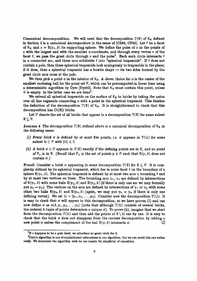
Canonical decomposition. We will need that the decomposition 'J(R) of KR defined in Section 3 is a canonical decomposition in the sense of [CS89, CF90]. Let f be a facet of KR and 5 = B(plt &) its supporting sphere. We define the poles of 5 as the points of 5 with the largest and with the smallest z-coordinate, and through every vertex v of the facet f, we pus the great circle through v and the polesl

. Each such circle intersects f in a connected arc, and these arcs subdivide f into "spherical trapezoids". If f does not contain a pole, then these spherical trapezoids look analogously to trapezoids in the plane; if it does, then a spherical trapezoid has a bowtie shape - its two sides formed by the great circle arcs cross at the pole.

We then pick a point 0 in the interior of KR. A clever choice for 0 is the center of the smallest enclosing ball for the point set P, which can be precomputed in linear time using a deterministic algorithm by Dyer [Dye92]. Note that KR must contain this point, unless K is empty. In the latter case we are done2

•

We extend all spherical trapezoids on the surface of KR to bricks by taking the union over all line segments connecting 0 with a point in the spherical trapezoid. This finishes the definition of the decomposition 'J(R) of KR. It is straightforward to check that this decomposition has 0URI) bricks.

Let !f denote the set of all bricks that appear in a decomposition 'J(R) for some subset R~ P.

Lemma 4 The decomposition 'J(R) defined above is a canonical decomposition ofKR in the fonowing sense:

(i) Every brick 0' is defined by at most five points, i.e. 0' appears in 'J(U) for some subset U C P with lUI ~ 5.

(li) A brick 0' E !f appears in 'J(R) exactly if the defining points are in R, and no point ofPu is in R. (Recall that PO" is the set of points PEP such that B(p,&) does not contain 0'.)

Proof: Consider a brick 0' appearing in some decomposition 'J(R) for R ~ P. It is com­pletely defined by its spherical trapezoid, which lies in some facet f on the boundary of a sphere B (p I, &). The spherical trapezoid is defined by at most two arcs "y bounding f and by at most two vertices on them. The bounding arcs "Yl, "Y2 are defined by intersections of B(Pl, &) with some balls B(P2, &) and B(P3, &) (if there is only one arc we may formally put P3 = P2)' The vertices on the arcs are defined by intersections of "Yl or "Y2 with some other two balls B(P4, &) and B(ps, &) (again, we may put Ps = P4 if there is only one defining vertex). We set U = {PI, P2 •... , Ps}. Consider now the decomposition 'J(U). It is easy to check that 0' will appear in this decomposition, so we have proven (i) and can now define 0' as 0'(&,Pl,P2,""Ps) (note that although 'J(U) consists of several bricks, the ordered 5-tuple of points determines a unique 0'). To prove (ii), imagine that we start from the decomposition 'J(U) and then add the points of R \ U one by one. It is easy to check that the brick 0' does not disappear from the current decomposition by adding a new point P unless the complement of the ball B(p, &) intersects 0'. Q]

lIf v happens to be a pole itself, we introduce no great circle for it. 2Dyer's algorithm is one of sophisticated subroutines in our algorithm, but we can avoid this one rather

easily. We formulate the algorithm with its use mainly for simplicity of exposition.

6

Linearization lemma. On several places of the proof of Lemma 3, we will deal with rather complicated predicates involving nonlinear polynomial inequalities. The main ex­ample will be the predicate "is C1 contained in B(p,5)?", where C1 is a brick, PEP is a point and 5 > 0 is a real parameter. Using an observation of Yao and Yao [YYSS], we can nevertheless deal with such predicates using techniques for "linear" objects (points and hyperplanes), by "lifting" the problem into a suitable space of higher dimensions. A precise formulation is given in the following lemma. Let us call a subset of R d a linear cell, if it can be expressed as a union of O( 1) sets, each of which is an intersection of 0(1) halfspaces in Rd.

Lemma 6 Let n(XI, X2, ... , Xk, aI, a2, ..• , at) be a first-order predicate in the theory of real closed fields (one formed from polynomial inequalities using Boolean connectives and quantifiers). Then there exists a constant d (depending on n) and mappings <P, '" as follows:

• The mapping <p assigns to every k-tuple x = (Xl, ... , Xk) a point <p(X) E Rd. The mapping is given by bounded-degree polynomials in Xl, ... , Xk.

• The mapping", assigns to every f-tuple a = (al, ... , ad a linear cell "'( a) ~ Rd. The functions describing the coef1icients in equations ofthe halfspaces defining "'( a) are given by bounded-degree polynomials in aI, a2, ... , at.

• For any a, x, n(x, a) holds iff the point <p(x) belongs to the linear cell "'(a).

Proof: The procedure for obtaining such mappings <p, '" is based on Yao and Yao's ob­servation and it is discussed in [Mat91]. First, we convert the formula for n into an equivalent quantifier-free formula (one composed of polynomial inequalities using Boolean connectives) using a quantifier elimination method, see e.g., [Ren92]. This formula can be rewritten as a disjunction of several conjunctions of polynomial inequalities.

We view the polynomials occurring in these inequalities as polynomials in the Xi vari­ables with coefficients being polynomials in the at variables. We let M be the set of all monomials J..l. = J..l.(x) in Xl, ... , Xk occurring in these polynomials. Then we set d = IMI, we imagine that the coordinates in R. d are indexed by the monomials of M, and we de­fine the mapping <p as follows: given a k-tuple X = (Xl, ..• , Xk) of real numbers, the point <p(x) = (YIJ.)IJ.EM E Rd is defined by YIJ. = J..l.(XI, ... , Xk) (the value ofthe monomial J..l. evalu­ated at the given k-tuple x). If we consider one polynomial inequality occurring in our for­mula, ofthe form LIJ.EM glJ.(a)J..l.(x) ~ 0 (each glJ. a polynomial in al, ... , at), it is satisfied for given x, a iff the point <p(x) lies in the halfspace {(YIJ.)IJ.EM E Rd j LIJ.EM glJ.(a)ylJ. ~ O}. A conjunction of several inequalities then corresponds to a membership of <p(x) in an intersection of several halfspaces, and a disjunction of several conjunctions corresponds to a union of several such intersections. The equations of the halfspaces are given by the 91J. polynomials in the ai variables and they can also be read off from the formula. g)

Point location method. As a first application of the above linearization lemma, we will discuss a way the subsets P (I as in Lemma 3 can be computed efficiently, when we already have the decomposition 'J(R) of the body KR into bricks.

7

A brick a can be described by specifying 6 and a vector ZI, ... , ZI5 of real parameters, expressing the five points defining a. We write a = 0'( 6, z). A point pER 3 is given by its three coordinates (UI, U2, U3). Then the predicate "a ~ B(p,6)" can be written as a first-order predicate in the variables 6, \4 and Zt (this is somewhat laborious but possible). Using Lemma 5 for this predicate, we get mappings cp,W as follows: cp = CP(6,UI,U2,U3) assigns to a value of 6 and a point p = (UI, U2, U3) a point in Rd (for some perhaps large but constant-bounded d), W = W(z) assigns to a parameter vector Z a linear cell in Rd, and a(6,z) ~ B(p, 6) is equivalent to cp(6, Ult U2, U3) E W(z).

We use these mappings for computing the sets P u (given the set P and the decompo­sition 'J(R» as follows. For every brick a E 'J(R), a = a(6,z), we compute the set W(z) (note that this is independent of 6). Then we preprocess the arrangement of these sets in Rd for all a E 'J(R) for fast point location. This can be done by preprocessing the full arrangement of all hyperplanes defining our sets for point location (several methods for point location in hyperplane arrangements are known, see e.g., [Cha92]). This yields a data structure with space and preprocessing time polynomial in I'J(R)I, thus, for ~ small enough, no more than linear in n. The query time will be o (log n). Then, for every point PEP, we locate the point cp (6, p) using this data structure, which tells us to which sets Pu does p belong. The total time will be O(nlogn). As for the oracle calls, each step of a point location query with some point p involves a comparison of the point cp(6,p) against some (explicitly known) hyperplane, and such a comparison can be decided by a bounded number of oracle calls. Since the n point location queries are independent and can be executed in a pseudo-parallel fashion, the total number of oracle calls is O(log2 n).

A quite similar approach can be used to compute the subset Qu. Here we need a data structure for location of points in the decomposition 'J(R). We apply Lemma 5 on the predicate ceq E a" (for a point q and a brick a = 0'( 6, z)), and we build a point location structure in the same manner as above. The set Qu can thus be detected in O(mlogn) time with O(log mlog n) oracle calls. Let us remark that an alternative - and perhaps more natural - way is to use a planar point location structure for point location in 'J(R), and then discuss how such a data structure is "parameterized" with 6, so that the preprocessing and point location queries only need a small number of oracle calls.

Computing a good sample in polynomial time. It remains to describe how to compute the "good" sample R. First we prove a weaker statement, namely that a suitable R can be found in polynomial time.

Lemma 6 Let P be a set of n points, r < n be a given parameter and let the parameter 6 > 0 be given as an oracle. We can identify in polynomial deterministic time a subset R of P such that

(i) IRI ~ r,

(li) for all aE 'J(R) wehavenu ~ cdn/r)logr, and

(ill)

8

for constants Cl, C2 > O. The number of calls to the oracle describing 5 is in O(logn). Within the same bounds we can compute the combinatorial structure of KR •

Proof: We appeal to the usual randomization results ([CS89]) to conclude that when an r-e1ement subset R is chosen randomly from P, the bounds in the lemma will hold with a positive probability. Applying derandomization techniques (i.e. the Raghavan-Spencer method) as in [CF90, Mat91a], we can then find a subset R that fulfills the requirements of the lemma in p·olynomial time.

To be more specific, let us use the result from [CF90]. To this end, we consider the hypergraph (P, 8), where 8 is the set of all subsets 5 of P which can be defined as

5 = {p E P; a g; B(p, 5)L

for some brick a which occurs in the canonical decomposition 'J(R) for some subset R ~ P. Lemma 4 implies that the number of such a is only polynomial in IPI (since each one is determined by an at most five-element subset of P). Given this hypergraph (explicitly), [CF90] shows that a sample R satisfying (i)-(iii) can be computed in polynomial time. We thus only need to compute the hypergraph (P,8) in polynomial time and with O(logn) oracle calls. This is not difficult, as we do not care for the exponent of the polynomial bounding the running time. Namely, we list all at most five-element subsets U of P, and for every such U we determine the bricks in the canonical decomposition corresponding to it. For every such brick, we then compute the subset of points of P defined by it. All the comparisons involving 5 are independent and can be done in a single round, thus O(logn) oracle calls suffice to resolve all of them. The rest of the calculations only deals with the hypergraph and requires no more information about 5.

The combinatorial structure of KR and its decomposition 'J(R) can be determined by one more round of polynomially many (in r) independent oracle calls. This proves Lemma 6. g]

Computing an approximation. Now that we can compute a suitable sample in polynomial time, we first compute a sufficiently small subset A of P that "approximates" P so well that it will be sufficient to apply Lemma 6 to A instead of P. This trick has been used in several previous works, see [Mat9la].

We consider a set system (P, 8), where 8 is defined similarly as in the proof of Lemma 6; a set 5 ~ P belongs to 8 if it can be expressed as the subset of points of P whose balls of radius p do not completely contain a certain brick a. The difference to the above proof is that we consider all radii p simultaneously, instead of a single value p = 5. Hence the set system (P, 8) does not depend on 5.

A subset A ~ P is called a (1 Ir )-approximation for (P, 8), if for any 5 E 8 we have

I

IA n 51 _ 13 1 ~ ! IAI IPI '" r'

Suppose that A is a (l/r)-approximation for (P,8), where r := not is as in Lemma 3. Let R ~ A be a subset with at most r elements satisfying the conditions (ii),(iii) of Lemma 3 with P replaced by A (and for some value of 5), that is, IAal ~ Cl (lAl/r) logr for every

9

0' E 'J(R) and LaE'.T(R) IAal ~ c21AI, Cl I C2 constants. For any brick 0', we have Pa E S (by the definition of the set system (P,S)), and Aa = An Pa. It is then straightforward to verify, using the definition of a (1 Ir )-approximation, that the subset R ~ A ~ P also ful:fi.lls the conditions (ii),(iii) of Lemma 3 for P, only with somewhat larger constants Cl, C2. To prove Lemma 3, we proceed as follows. First, given P, we compute a (l/r)-approximation A for the set system (P,S), with IAI much smaller than n = IPI. Then we apply Lemma 6 with A in the role of P, and we find a good sample R. By the above considerations, this R will also be good with respect to P. However, since A is small enough, we can afford to spend time bounded by a polynomial in IAI. The proof of Lemma 3 is finished by computing the decomposition 'J(R) (all the combinatorial information needed for this can be gained by a single round of independent oracle calls, thus by O(logn) actual oracle calls) and detecting the subsets Pa and Qa for every 0' E 'J(R); this has already been discussed above.

It remains to describe how the (1 Ir )-approximation A is computed. Here we again ap­ply the "linearization" method, Lemma 5. Our predicate will be "0' ~ B(p, p)", 0' = O'(p, z) a brick and p a point. This time, however, we will regard only the coordinates of the point p in the role of the Xi variables in Lemma 5, both z and p will be regarded as the at vari­ables. We thus obtain a mapping cp assigning to a point p E R3 a point cp(p) E Rd (for some constant d) and a mapping W assigning to every z and p a linear cell in Rd, in such a way that for any p, p,Z, O'(p,z) ~ B(p, p) iff cp(p) E W(Z, pl. Returning to our set system (P, S), we see that every S E S can be expressed as those points of P whose cp-image lies in a certain linear cell in Rd. Since every linear cell can be written as a disjoint union of at most C simplices (C a suitable constant), it suffices to compute a (l/Cr)-approximation for the set {cp(p); PEP} with all its subsets definable by simplices. For this last problem, we can directly use the results of [Mat92], and we get that if a. > 0 is a small enough constant, our (l/r)-approximation A of size O(r2Iogr) can be computed in O(nlogn) time. This calculation does not involve the parameter b at all. This finishes the proof of Lemma 3. Q]

References

[Cha92] B. Chazelle. Cutting hyperplanes for divide-and-conquer. Discrete fJ Compu­tational Geometry, 1992. To appear. Preliminary version: Proc. 92nd IEEE Symposium on Foundations of Computer Science (1991).

[CEGS92] B. Chazelle, H. Edelsbrunner, L. Guibas, and M. Sharir. Diameter, width, closest line pair, and parametric searching. In Proc. 8th Annu. ACM Sympos. Comput. Geom., pages 120-129,1992.

[CF90] B. Chazelle and J. Friedman. A deterministic view of random sampling and its use in geometry. Combinatorica, 10:229-249, 1990.

[CS89] K. L. Clarkson and P. W. Shor. Applications of random sampling in computa­tional geometry II. Discrete fJ Computational Geometry, 4:387-421, 1989.

10

[Dye92] M. Dyer. A class of convex programs with applications to computational ge­ometry. In Proc. 8th Annu. ACM Sympos. Comput. Geom., pages 9-15, 1992.

[Mat91] J. Matousek. Cutting hyperplane arrangements. Discrete €J Computational Geometry, 6(5):385-406, 1991.

[Mat91a] J. Matousek. Approximation and geometric divide and conquer. In Proc. 29m Annu. ACM Sympos. Theory Comput., pages 505-511, 1991.

[Mat92] J. Matousek. Efficient partition trees. Discrete €J Computational Geometry 8:315-334 (1992).

[Meg83] N. Megiddo. Applying parallel computation algorithms in the design of serial algorithms. Journal of the ACM, 30:852-865,1983.

[Ren92] J. Renegar. On the computational complexity and geometry of the first order theory of the reals. Journal of Symbolic Computation, 1992.

[YY85] F. F. Yao and A. C. Yao. A general approach to geometric queries. In Proc. 17. ACM Symposium on Theory of Computing, pages 163-168, 1985.

11