a desire support - gondola...

A Desire Named Streetcar Fantasy and Fact in Rail Transit Planning Don H. Pickrell

The forecasts that led local officials in eight U.S. cities to advocate rail transit projects over competing, less capital-intensive options grossly overestimated rail transit ridership and under- estimated rail construction costs and operating expenses. These mistakes cannot be explained by such obvious sources as errors in projecting the input variables of the ridership forecasting models, or changes in the design of projects. Although planners could reduce the magnitude of the errors by various technical improvements in the forecasting process, the structure of transit grant programs and the existence of dedicated funding sources provide little incentive for local officials to seek accurate information in evaluating alternatives. The resulting bias toward high-capital transit investments is thus unlikely to be eliminated without restructuring both federal transit grant programs and local financing mechanisms.

Pickrell is an economist at the John A. Volpe National Transportation Systems Center, U.S. Department of Transportation. He was previously on the faculty of city and regional planning at Harvard and in civil engineering at MIT. His research focuses on planning and public policy issues in urban transportation.

Journal of the American Planning Association, Vol. 58, No. 2, Spring 1992. OAmerican Planning Association, Chi- cago, IL.

Federal Support for Rail Transit During the past three decades, the federal government

has invested $60 billion in an attempt to reverse public transit’s declining role in the nation’s urban transportation system. Nearly a quarter of this largess has been used by its local beneficiaries to finance construction of new rail transit lines. Over this period, the Urban Mass Trans- portation Administration (UMTA)-the agency responsible for allocating federal transit support-has developed an increasingly formalized process for local agencies to use in formulating alternative projects and selecting a favored candidate for which to seek funding. In this process, local officials choose among competing alternatives by weighing the improvement in transit service and the increase in transit ridership forecast to result from each project against its anticipated cost to construct and operate.

This paper assesses the accuracy of forecasts of ridership and costs that led local officials in each of eight U.S. cities to select a rail transit project over other options. The paper focuses upon the accuracy of forecasts that were available to decision makers at the time they chose among alternative projects. Although officials often subsequently revised these projections to reflect higher costs and lower ridership, in no case did they reconsider their earlier decision in light of these more realistic estimates.’ The accuracy of the decision-date forecasts reflects the extent to which expectations raised by planners of these projects and used by advocates to promote them have been achieved, rather than whether the projects represented sensible investments. While these two issues- the reliability of forecasts and the desirability of these investments-are obviously related, this paper is concerned solely with assessing how closely actual experience has accorded with planners’ expectations, rather than with evaluating specific projects or assessing whether subsidies to construct rail transit should remain a cornerstone of national transportation policy.

Why Does Accuracy Matter? There are several reasons to be concerned about the

accuracy of forecasts prepared to support transit investment decisions. First, virtually every project this article reviews represented the largest investment in public works ever undertaken by the local area, often by a con- siderable margin. Another nineteen U.S. cities are now considering major transit projects, many of which are again by far the largest scale public investments these municipalities have ever contemplated. Thus it certainly seems worthwhile to assess the process they use in planning and evaluating these projects. Perhaps the most obvious dimension of such an assessment is evaluating how closely the actual benefits of the projects have matched the expectations that led local planners and politicians to select them.

Second, local officials continue to choose-almost always in favor of a rail line-among alternative transit projects on the basis of narrow margins among their pro-

APA JOURNAL 158 SPRING 1992

jected costs and fidership. While local officials also weigh political and environmental factors in making these decisions, the preferred option must still be demonstrably more cost effective in promoting transit ridership than any of the rejected alternatives to be eligible for federal funding. The viability of a planning process in which officials predicate major decisions (or, having based these decisions on other factors, find it convenient to defend them) on small differences in the projected future values of a few important variables depends critically on how errors in forecasting these variables compare to the magnitude of these differences. If forecasting errors are large in comparison to variation among competing projects’ estimated costs and ridership, the process cannot be relied upon to guide decision makers toward sensible choices. A wide margin of forecasting error may also signal analysts’ complicity in demonstrating the purported technical superiority of projects that could not prevail in an unbiased evaluation, but are favored by influential local officials for other-often unspoken-reasons.

Finally, local officials typically use a similar process to plan many other major public infrastructure investments: Analysts weigh the anticipated effectiveness of alternative projects in meeting stated objectives against differences in projected costs.* In fact, the current process almost perfectly embodies the rational planning model of planning theory. And as actually implemented, the process closely resembles the hybrid of political and technical considerations often advocated in the academic planning literature (Wachs 1985; Meyer and Miller 1984; and Johnston et al. 1988), particularly in its recognition of the necessity to structure a local consensus that in- corporates political and environmental considerations, but is also defensible on strictly economic concerns. Not only does the transit planning process thus represent an example worth careful study but it also provides a more

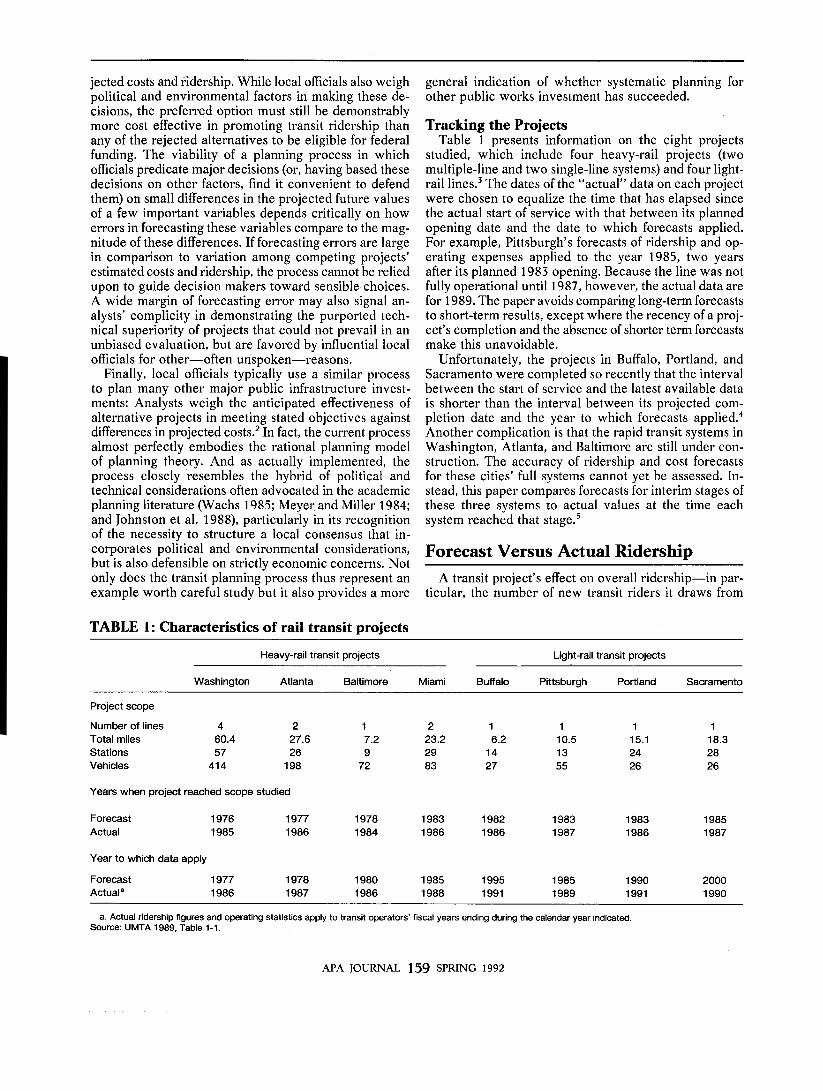
TABLE 1 : Characteristics of rail transit projects

general indication of whether systematic planning for other public works investment has succeeded.

Tracking the Projects Table 1 presents information on the eight projects

studied, which include four heavy-rail projects (two multiple-line and two single-line systems) and four light- rail lines.3 The dates of the “actual” data on each project were chosen to equalize the time that has elapsed since the actual start of service with that between its planned opening date and the date to which forecasts applied. For example, Pittsburgh‘s forecasts of ridership and operating expenses applied to the year 1985, two years after its planned 1983 opening. Because the line was not fully operational until 1987, however, the actual data are for 1989. The paper avoids comparing long-term forecasts to short-term results, except where the recency of a project’s completion and the absence of shorter term forecasts make this unavoidable.

Unfortunately, the projects in Buffalo, Portland, and Sacramento were completed so recently that the interval between the start of service and the latest available data is shorter than the interval between its projected completion date and the year to which forecasts a ~ p l i e d . ~ Another complication is that the rapid transit systems in Washington, Atlanta, and Baltimore are still under construction. The accuracy of ridership and cost forecasts for these cities’ full systems cannot yet be assessed. In- stead, this paper compares forecasts for interim stages of these three systems to actual values at the time each system reached that stage.5

Forecast Versus Actual Ridership A transit project’s effect on overall ridership-in par-

ticular, the number of new transit riders it draws from

Heavy-rail transit projects Light-rail transit projects

Washington Atlanta Baltimore Miami Buffalo Pittsburgh Portland Sacramento

Project scope

Number of lines 4 2 1 2 1 1 1 1 Total miles 60.4 27.6 7.2 23.2 6.2 10.5 15.1 18.3 Stations 57 26 9 29 14 13 24 28 Vehicles 414 198 72 83 27 55 26 26

Years when project reached scope studied

Forecast 1976 1977 1978 1983 1982 1983 1983 1985 Actual 1985 1986 1984 1986 1986 1987 1986 1987

Year to which data apply

Forecast 1977 1978 1980 1985 1995 1985 1990 2000 Actuala 1986 1987 1986 1988 1991 1989 1991 1990

a. Actual ridership figures and operating statistics apply to transit operators’ fiscal years ending during the calendar year indicated. Source: UMTA 1989, Table 1-1.


DON H. PICKRELL

automobiles-is the primary determinant of its success in alleviating traffic congestion, reducing air pollution, and achieving the variety of other objectives sought by local officials who elected to build rail lines. Hence, actual ridership that consistently differs from forecast levels indicates that the benefits stemming from these investments diverge from those that led local officials to select them.

Figure 1 compares the forecast and actual numbers of daily passengers on each line or system-the most widely cited, although not necessarily the most informative, in- dicator of the anticipated and actual use of a new transit facility. Only Washington’s extensive Metrorail system experiences actual ridership that is more than one-half of its forecast level; the number of passengers it carried during 1986 was 28 percent below expected use of a nearly identical system projected to operate during 1977. Ridership on Washington’s rail system compares favorably to its forecast level partly because employment in the city’s downtown, the single most important demographic influence on transit ridership, increased nearly 25 percent during the nine-year delay in the system’s construction.6

Figure 1 shows even less favorable comparisons between forecast and actual rail ridership in other cities: Actual patronage on new lines in Baltimore and Portland is somewhat below one-half of that forecast, while in all other cases actual ridership is less than one-third of its o,e:n:,otnA 1,,,,1 /Rnnn..rn AK,.:nlo ,.-,.A -:A---L:-

Buffalo, Portland, and Sacramento include as many as 20 percent who are traveling within free or reduced-fare zones within these cities’ downtowns, but who were not included in forecasts of r ider~hip.~ In Pittsburgh, reported ridership includes passengers on a trolley line operating parallel to its light-rail line, while the forecast was only for ridership on the light-rail line.

Total Transit Ridership While the number of total passengers measures the

intensity of use of a new rail service, it is a somewhat misleading index of the match between project benefits and planners’ expectations. This is because rail ridership typically consists primarily of former bus travelers, and only secondarily of former auto users and those making entirely new trips. Both the nature and level of benefits to these distinct groups differ. While former bus riders may benefit from improved service on new rail lines, only to the extent that rail lines divert auto drivers to transit travel do the lines reduce traffic congestion, air pollution, and other undesirable by-products of automobile travel-usually the local officials’ most important stated reason for selecting rail projects over competing alternatives. Thus, a more accurate reflection of the ma- terialization of the projects’ expected benefits is the comparison of anticipated and actual increases in areawide transit ridership accompanying new rail lines.

Unfortunately, planners do not always prepare fore- -,.”4” ,.P _-,.-- .cL :- .-:A,..--L:.- ,.-,I 4L- P.-,.,.4:-... -L- _--_ -.*:A,..--

A DESIRE NAMED STREETCAR

800

600

u)

P I

e 400

200

0

Forecasl la Actual

Washington Atlanta Miami Buffalo Pittsburgh Portland Sacramento

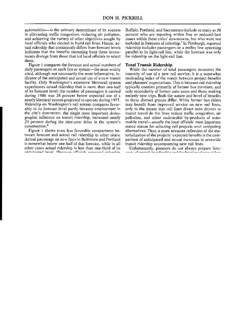
(combined bus and rail use) with each new line (or system) in operation.8 It shows that actual ridership on bus and rail service together is below its forecast level in six of seven urban areas, most often by a substantial margin. (Baltimore had no forecast of total ridership.) The prom- inent exception is Atlanta, where the average number of weekday transit trips during 1987-when about one-half of its planned rail system was in operation-was 8 percent above that forecast for 1978, when the system was originally expected to reach this scope. Another bright note is Washington, where actual transit ridership was within 12 percent of the forecast for 1977, when the city was originally scheduled to be served by the system that operated during 1986.

In both Atlanta and Washington, however, this comparison is artificially favorable because of the influence on transit ridership of growth in downtown employment and population between the time each city’s rail system was projected to become this extensive and the date when this actually occurred. Figure 2 also paints a contrasting picture in other cities: Actual transit ridership is roughly one-half of that expected to accompany the operation of light-rail service in Buffalo, Pittsburgh, and Portland, about one-third of that forecast in Sacramento, and only about one-quarter of its projected level in Miami.

Why Do Forecast and Actual Ridership Differ? Although urban travel demand forecasting is not an

exact science, the process had already become quite so- phisticated when analysts produced the ridership forecasts for the earliest rail projects represented in this study.g Usually transit patronage forecasts are the product of a sequence of models analysts use to study and predict

FIGURE 2: Weekday transit trips on bus and rail.

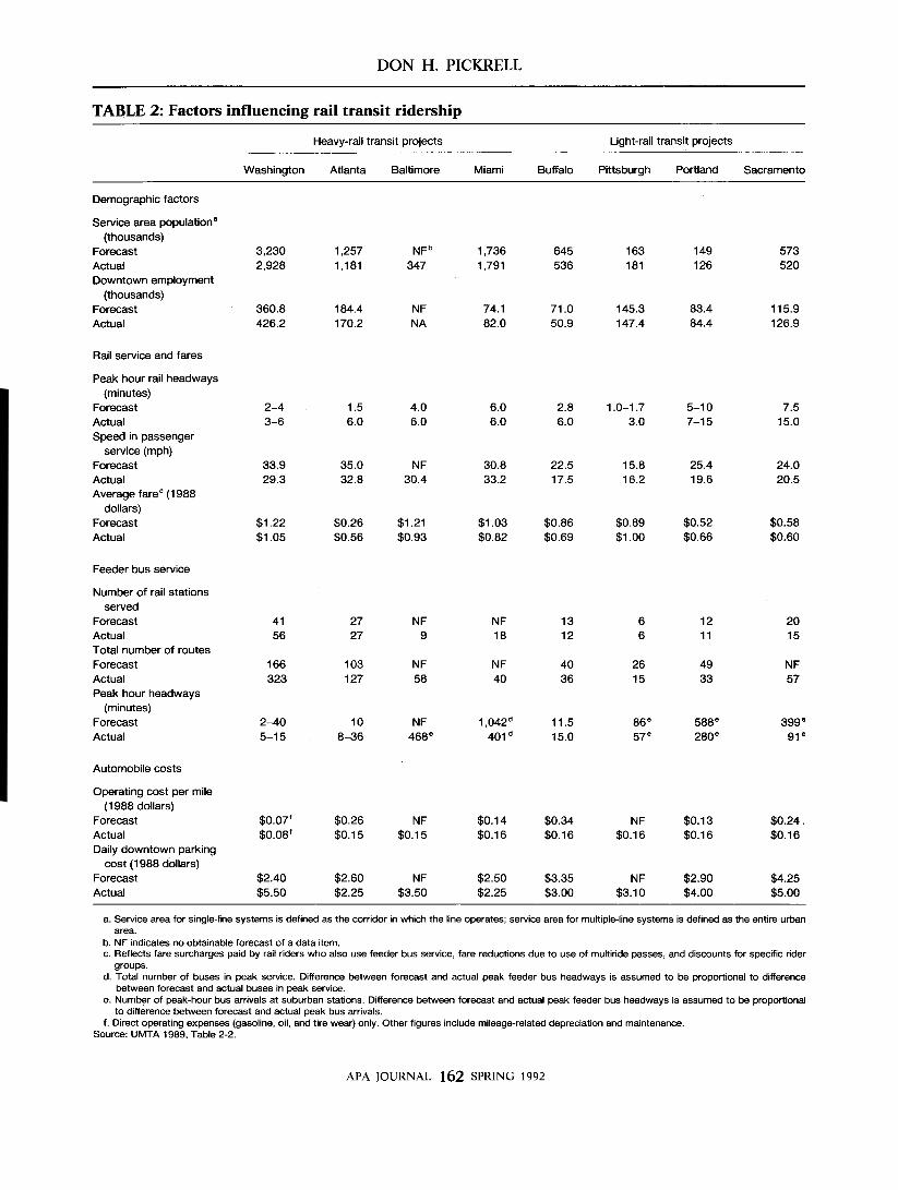
aggregate travel volume in an urban area, the spatial distribution of trip-making, the levels of transit travel in specific corridors, and ultimately patronage on specific routes or services. Errors in forecasting outputs can arise because analysts incorrectly forecast exogenous inputs, the structure of models inaccurately reflects actual travel behavior, or their application in the forecasting process introduces errors. The critical inputs into forecasting ridership on a proposed rail line include three basic categories: demographic factors such as downtown employment and population in the corridors where lines are to be located; the level of transit service lines are expected to provide, including the frequency and speed of rail service together with the extent of feeder bus service to rail transit stations, as well as the fare to be charged; and the speed, cost, and convenience of operating and parking automobiles, which represent the major competing mode of travel. Table 2 compares the forecast values of demographic factors, transit service levels and fares, and auto costs to their actual values in the eight cities that built these projects.

The table indicates that forecasts of the two basic demographic variables influencing travel volumes-population and downtown employment-generally compared quite closely to their actual values in the areas served by new rail projects. Only the overestimates of future corridor population and downtown employment in Buffalo appear sufficient to contribute significantly to overestimation of future ridership. Although the actual frequency of rail service during peak travel periods falls well short of that forecast in several cases, in the actual headways most are still within a range that passengers are probably willing to arrive randomly at stations be-


DON H. PICKRELL

TABLE 2: Factors influencing rail transit ridership



Demographic factors

Service area population'

Forecast Actual Downtown employment

Forecast Actual

(thousands)

(thousands)

Rail service and fares

Peak hour rail headways

Forecast Actual Speed in passenger

Forecast Actual Average fare' (1988

dollars) Forecast Actual

(minutes)

service (mph)

Feeder bus service

Number of rail stations SeNed

Forecast Actual Total number of routes Forecast Actual Peak hour headways

Forecast Actual

(minutes)

Automobile costs

Operating cost per mile

Forecast Actual Daily downtown parking

cost (1 988 dollars) Forecast Actual

(1 988 dollars)

3,230 2,928

360.8 426.2

2-4 3-6

33.9 29.3

$1.22 $1.05

41 56

166 323

2-40 5-1 5

$0.07' $0.08'

$2.40 $5.50

1,257 1,181

184.4 170.2

1.5 6.0

35.0 32.8

$0.26 $0.56

27 27

103 127

10 8-36

$0.26 $0.1 5

$2.60 $2.25

N F ~ 347

NF NA

4.0 6.0

NF 30.4

$1.21 $0.93

NF 9

NF 58

NF 468"

NF $0.15

NF $3.50

1,736 1,791

74.1 82.0

6.0 6.0

30.8 33.2

$1.03 $0.82

NF 18

NF 40

1,042' 401 '

$0.14 $0.16

$2.50 $2.25

645 536

71 .O 50.9

2.8 6.0

22.5 17.5

$0.86 $0.69

13 12

40 36

11.5 15.0

$0.34 $0.16

$3.35 $3.00

163 181

145.3 147.4

1 .o-1.7 3.0

15.8 16.2

$0.89 $1 .oo

6 6

26 15

86= 57*

NF $0.16

NF $3.10

149 126

83.4 84.4

5-1 0 7-1 5

25.4 19.6

$0.52 $0.66

12 11

49 33

588e 280"

$0.13 $0.16

$2.90 $4.00

573 520

115.9 126.9

7.5 15.0

24.0 20.5

$0.58 $0.60

20 15

NF 57

399" 91 *

$0.24 $0.16

$4.25 $5.00

a. Service area for single-line systems is defined as the corridor in which the line operates: service area for multiple-line systems is defined as the entire urban

b. NF indicates no obtainable forecast of a data item. c. Reflects fare surcharges paid by rail riders who also use feeder bus service, fare reductions due to use of multiride passes, and discounts for specific rider

d. Total number of buses in peak service. Difference between forecast and actual peak feeder bus headways is assumed to be proportional to difference

e. Number of peak-hour bus arrivals at suburban stations. Difference between forecast and actual peak feeder bus headways is assumed to be proportional

f. Direct operating expenses (gasoline, oil, and tire wear) only. Other figures include mileage-related depreciation and maintenance.

area.

groups.

between forecast and actual buses in peak service.

to difference between forecast and actual peak bus arrivals.

Source: UMTA 1989, Table 2-2.



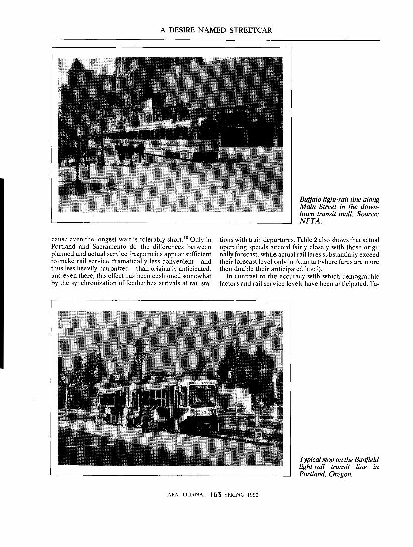
Buffalo light-rail line along Main Street in the downtown transit mall. Source: NFTA.

cause even the longest wait is tolerably short." Only in Portland and Sacramento do the differences between planned and actual service frequencies appear sufficient to make rail service dramatically less convenient-and thus less heavily patronized-than originally anticipated, and even there, this effect has been cushioned somewhat by the synchronization of feeder bus arrivals at rail sta-

tions with train departures. Table 2 also shows that actual operating speeds accord fairly closely with those originally forecast, while actual rail fares substantially exceed their forecast level only in Atlanta (where fares are more then double their anticipated level).

In contrast to the accuracy with which demographic factors and rail service levels have been anticipated, Ta-


Typical stop on the Banfield light-rail transit line in Portland, Oregon.

DON H. PICKRELL

ble 2 shows that actual feeder bus service to suburban stations has more often fallen short of its forecast level. This difference seems likely to contribute most to ex- plaining the gap between forecast and actual rail ridership in Miami, where the number of buses operating in feeder service during peak periods is only about 40 percent of that originally anticipated; feeder service also appears significantly lower than originally planned in Sacramento. Finally, the table suggests that assumptions about the future cost of operating and parking automobiles probably did not contribute significantly to the large errors in forecasting rail ridership. While concern over escalating energy prices during the 1970s apparently led planners to substantially overestimate future auto operating costs in a few cases (Atlanta, Buffalo, and Sacramento), future downtown parking prices-a far more important determinant of transit use-were often seriously underesti- mated.

Calculations using travel demand elasticities suggest that the errors documented in Table 2 explain less than one-half of the observed gap between predicted and actual rail boardings in every case except Buffalo, where they appear sufficient to account for the entire difference.” In the few other cases where a significant share of this gap can be explained by errors in forecasting these inputs, the differences between projected and actual ridership are so large that a substantial absolute gap still remains unexplained. Instead, errors must have arisen from other less obvious sources, such as the structure of the forecasting models, how they were employed, or the misinterpretation-or possibly misrepresentation-of their numerical outputs.” Errors in projecting future ridership also appear to be increasing rather than declining

over time, suggesting that technical deficiencies in past forecasting models were not a major source of error. Thus, the refinements in the structure of these models that have been demanded by forecasting critics and ac- claimed by its practitioners have not by themselves led to more accurate f0re~asts . l~

Capital Outlays for Rail Transit Projects

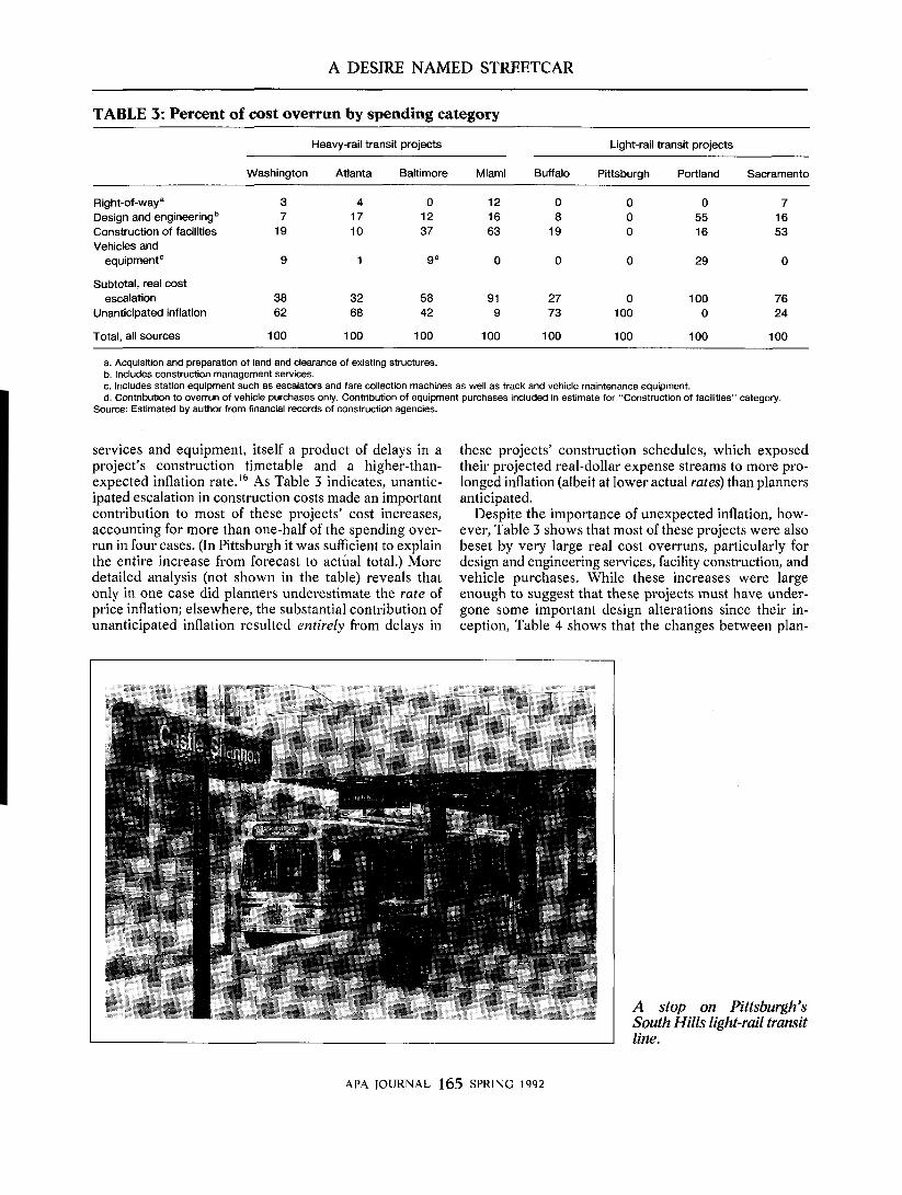
As Figure 3 shows, actual capital outlays for seven of the eight rail transit projects reviewed were typically well above those foreca~t . ’~ (Pittsburgh did not prepare a specific forecast of actual cost outlays.) Capital spending overruns ranged from 17 percent for Sacramento’s light- rail line to more than 150 percent for the first sixty miles of Washington’s Metro system. These differences capture the effects not only of errors in estimating the real economic cost of the construction services and other resources utilized by each project, but also of errors in financial planning, which includes such activities as construction scheduling, project management, and forecasting the pace of price inflation. Table 3 shows the separate contributions of five different spending categories to the nominal-dollar cost overruns shown in Figure 3. Four of these categories are denominated in constant or real dollars: right-of-way acquisition and preparation; design, engineering, and project management services: construction of lines, stations, and other facilities: and vehicle and equipment purchase^.'^

The error in projecting nominal-dollar outlays consists of these four real-dollar categories plus the effect of unanticipated inflation in prices for construction-related

~~~~

5000

4000

3000

2000

1000

0

Forecast Actual

Washington Atlanta Baltimore Miami Buffalo Portland Sacramento FIGURE 3: Forecast and actual capital outlays in nominal dollars.

APA IOURNAL 164 SPRING 1992


TABLE 3: Percent of cost overrun by spending category



Right-of-waya 3 4 0 12 0 0 0 7 Design and engineeringb 7 17 12 16 8 0 55 16 Construction of facilities 19 10 37 63 19 0 16 53 Vehicles and

equipment” 9 1 gd 0 0 0 29 0

Subtotal, real cost escalation 38 32 58 91 27 0 100 76

Unanticipated inflation 62 68 42 9 73 100 0 24

Total, all sources 100 100 100 100 100 100 100 100 _____

a. Acquisition and preparation of land and clearance of existing structures. b. Includes construction management services. c. Includes station equipment such as escalators and fare collection machines as well as track and vehicle maintenance equipment. d. Contribution to overrun of vehicle purchases only. Contribution of equipment purchases included in estimate for “Construction of facilities” category.

Source: Estimated by author from financial records of construction agencies.

services and equipment, itself a product of delays in a project’s construction timetable and a higher-than- expected inflation rate.16 As Table 3 indicates, unanticipated escalation in construction costs made an important contribution to most of these projects’ cost increases, accounting for more than one-half of the spending overrun in four cases. (In Pittsburgh it was sufficient to explain the entire increase from forecast to actual total.) More detailed analysis (not shown in the table) reveals that only in one case did planners underestimate the rate of price inflation; elsewhere, the substantial contribution of unanticipated inflation resulted entirely from delays in

these projects’ construction schedules, which exposed their projected real-dollar expense streams to more pro- longed inflation (albeit at lower actual rates) than planners anticipated.

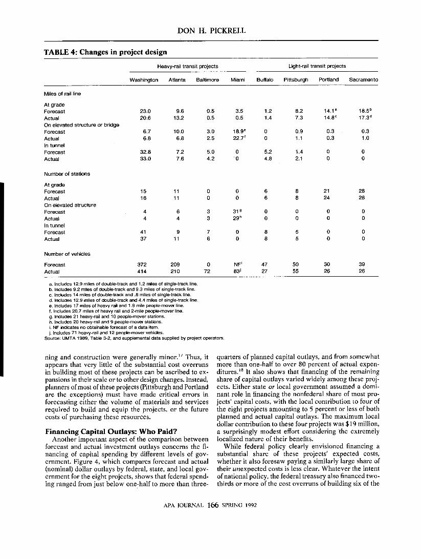
Despite the importance of unexpected inflation, however, Table 3 shows that most of these projects were also beset by very large real cost overruns, particularly for design and engineering services, facility construction, and vehicle purchases. While these increases were large enough to suggest that these projects must have under- gone some important design alterations since their in- ception, Table 4 shows that the changes between plan-


A stop on Pittsburgh’s South Hills light-rail transit line.

DON H. PICKRELL

TABLE 4: Changes in project design



Miles of rail line

At grade Forecast Actual On elevated structure or bridge Forecast Actual In tunnel Forecast Actual

Number of stations

At grade Forecast Actual On elevated structure Forecast Actual In tunnel Forecast Actual

Number of vehicles

Forecast Actual

23.0 20.6

6.7 6.8

32.8 33.0

15 16

4 4

41 37

372 41 4

9.6 13.2

10.0 6.8

7.2 7.6

1 1 1 1

6 4

9 11

209 21 0

0.5 3.5 1.2 8.2 14.1 a 18.5 0.5 0.5 1.4 7.3 14.8' 17.3'

3.0 18.ge 0 0.9 0.3 0.3 2.5 22.7' 0 1.1 0.3 1 .o

5.0 0 5.2 1.4 0 0 4.2 0 4.8 2.1 0 0

0 0 6 8 21 28 0 0 6 8 24 28

3 31 0 0 0 0 3 29 0 0 0 0

7 0 8 5 0 0 6 0 8 5 0 0

0 NF' 47 50 30 39 72 83' 27 55 26 26

a. Includes 12.9 miles of double-track and 1.2 miles of single-track line. b. Includes 9.2 miles of double-track and 9.3 miles of single-track line. c. Includes 14 miles of double-track and .8 miles of single-track line. d. Includes 12.9 miles of double-track and 4.4 miles of single-track line. e. Includes 17 miles of heavy rail and 1.9 mile people-mover line. f. Includes 20.7 miles of heavy rail and 2-mile people-mover line. g. Includes 21 heavy-rail and 10 people-mover stations. h. Includes 20 heavy-rail and 9 people-mover stations. i. NF indicates no obtainable forecast of a data item. j. Includes 71 heavy-rail and 12 people-mover vehicles.

Source: UMTA 1989, Table 3-2, and supplemental data supplied by project operators.

ning and construction were generally minor.I7 Thus, it appears that very little of the substantial cost overruns in building most of these projects can be ascribed to ex- pansions in their scale or to other design changes. Instead, planners of most of these projects (Pittsburgh and Portland are the exceptions) must have made critical errors in forecasting either the volume of materials and services required to build and equip the projects, or the future costs of purchasing these resources.

Financing Capital Outlays: Who Paid? Another important aspect of the comparison between

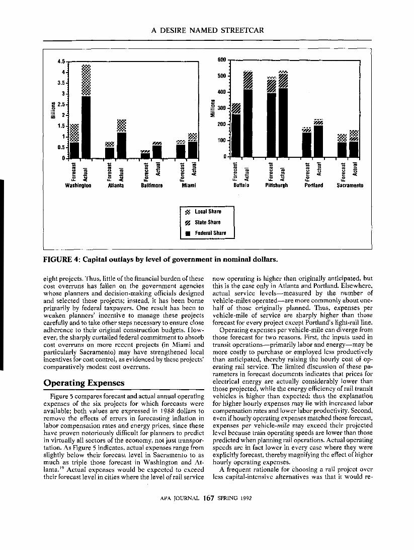
forecast and actual investment outlays concerns the financing of capital spending by different levels of government. Figure 4, which compares forecast and actual (nominal) dollar outlays by federal, state, and local government for the eight projects, shows that federal spending ranged from just below one-half to more than three-

quarters of planned capital outlays, and from somewhat more than one-half to over 80 percent of actual expenditures." It also shows that financing of the remaining share of capital outlays varied widely among these projects. Either state or local government assumed a domi- nant role in financing the nonfederal share of most projects' capital costs, with the local contribution to four of the eight projects amounting to 5 percent or less of both planned and actual capital outlays. The maximum local dollar contribution to these four projects was $19 million, a surprisingly modest effort considering the extremely localized nature of their benefits.

While federal policy clearly envisioned financing a substantial share of these projects' expected costs, whether it also foresaw paying a similarly large share of their unexpected costs is less clear. Whatever the intent of national policy, the federal treasury also financed two- thirds or more of the cost overruns of building six of the

APA IOURNAL 166 SPRING 1992


4.5

Washingtbn Atlanta Baltimore Miami Buffalo Pittsburgh Portland Sacramento

# State Share

Federalshare

FIGURE 4: Capital outlays by level of government in nominal dollars.

eight projects. Thus, little of the financial burden of these cost overruns has fallen on the government agencies whose planners and decision-making officials designed and selected these projects; instead, it has been borne primarily by federal taxpayers. One result has been to weaken planners' incentive to manage these projects carefully and to take other steps necessary to ensure close adherence to their original construction budgets. How- ever, the sharply curtailed federal commitment to absorb cost overruns on more recent projects (in Miami and particularly Sacramento) may have strengthened local incentives for cost control, as evidenced by these projects' comparatively modest cost overruns.

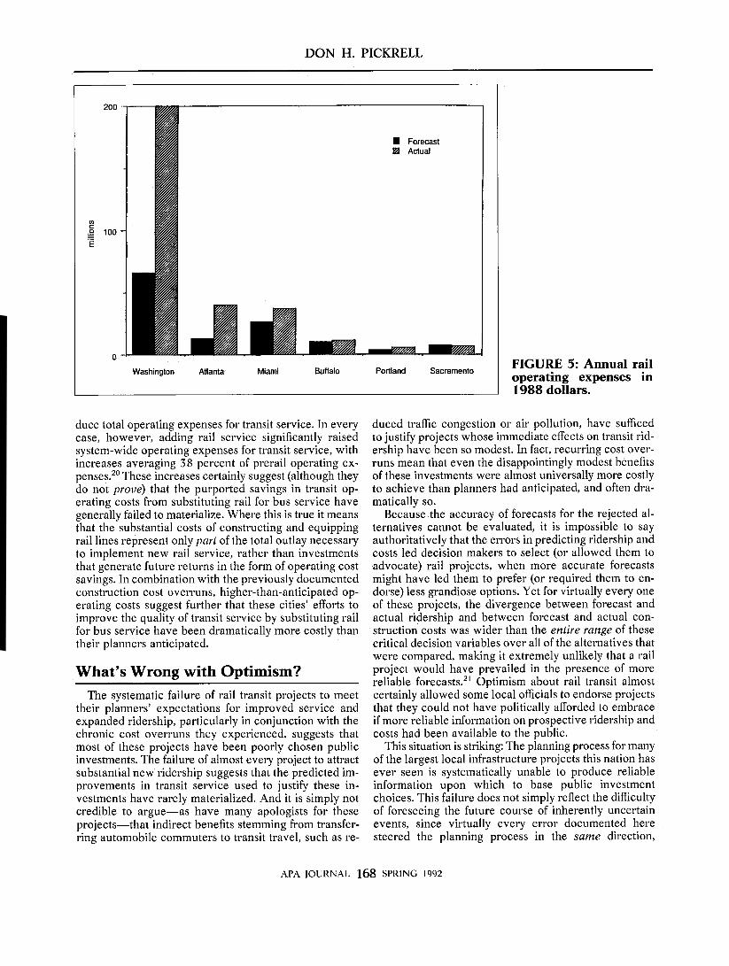
Operating Expenses Figure 5 compares forecast and actual annual operating

expenses of the six projects for which forecasts were available: both values are expressed in 1988 dollars to remove the effects of errors in forecasting inflation in labor compensation rates and energy prices, since these have proven notoriously difficult for planners to predict in virtually all sectors of the economy, not just transportation. As Figure 5 indicates, actual expenses range from slightly below their forecast level in Sacramento to as much as triple those forecast in Washington and At- lanta." Actual expenses would be expected to exceed their forecast level in cities where the level of rail service

now operating is higher than originally anticipated, but this is the case only in Atlanta and Portland. Elsewhere, actual service levels-measured by the number of vehicle-miles operated-are more commonly about one- half of those originally planned. Thus, expenses per vehicle-mile of service are sharply higher than those forecast for every project except Portland's light-rail line.

Operating expenses per vehicle-mile can diverge from those forecast for two reasons. First, the inputs used in transit operations-primarily labor and energy-may be more costly to purchase or employed less productively than anticipated, thereby raising the hourly cost of operating rail service. The limited discussion of these parameters in forecast documents indicates that prices for electrical energy are actually considerably lower than those projected, while the energy efficiency of rail transit vehicles is higher than expected; thus the explanation for higher hourly expenses may lie with increased labor compensation rates and lower labor productivity. Second, even if hourly operating expenses matched those forecast, expenses per vehicle-mile may exceed their projected level because train operating speeds are lower than those predicted when planning rail operations. Actual operating speeds are in fact lower in every case where they were explicitly forecast, thereby magnifying the effect of higher hourly operating expenses.

A frequent rationale for choosing a rail project over less capital-intensive alternatives was that it would re-


DON H. PICKRELL

Washington Atlanta. Miami Buffalo Portland Sacramento I FIGURE 5: Annual rail

duce total operating expenses for transit service. In every case, however, adding rail service significantly raised system-wide operating expenses for transit service, with increases averaging 3 8 percent of prerail operating expenses.” These increases certainly suggest (although they do not prove) that the purported savings in transit operating costs from substituting rail for bus service have generally failed to materialize. Where this is true it means that the substantial costs of constructing and equipping rail lines represent only part of the total outlay necessary to implement new rail service, rather than investments that generate future returns in the form of operating cost savings. In combination with the previously documented construction cost overruns, higher-than-anticipated operating costs suggest further that these cities’ efforts to improve the quality of transit service by substituting rail for bus service have been dramatically more costly than their planners anticipated.

What’s Wrong with Optimism? The systematic failure of rail transit projects to meet

their planners’ expectations for improved service and expanded ridership, particularly in conjunction with the chronic cost overruns they experienced, suggests that most of these projects have been poorly chosen public investments. The failure of almost every project to attract substantial new ridership suggests that the predicted improvements in transit service used to justify these investments have rarely materialized. And it is simply not credible to argue-as have many apologists for these projects-that indirect benefits stemming from transfer- ring automobile commuters to transit travel, such as re-

duced traffic congestion or air pollution, have sufficed to justify projects whose immediate effects on transit ridership have been so modest. In fact, recurring cost overruns mean that even the disappointingly modest benefits of these investments were almost universally more costly to achieve than planners had anticipated, and often dramatically so.

Because the accuracy of forecasts for the rejected alternatives cannot be evaluated, it is impossible to say authoritatively that the errors in predicting ridership and costs led decision makers to select (or allowed them to advocate) rail projects, when more accurate forecasts might have led them to prefer (or required them to endorse) less grandiose options. Yet for virtually every one of these projects, the divergence between forecast and actual ridership and between forecast and actual construction costs was wider than the entire range of these critical decision variables over all of the alternatives that were compared, making it extremely unlikely that a rail project would have prevailed in the presence of more reliable forecasts.” Optimism about rail transit almost certainly allowed some local officials to endorse projects that they could not have politically afforded to embrace if more reliable information on prospective ridership and costs had been available to the public.

This situation is striking: The planning process for many of the largest local infrastructure projects this nation has ever seen is systematically unable to produce reliable information upon which to base public investment choices. This failure does not simply reflect the difficulty of foreseeing the future course of inherently uncertain events, since virtually every error documented here steered the planning process in the same direction,



namely toward the most capital-intensive rail transit option under consideration. By tolerating pervasive errors of the consistent direction and extreme magnitude documented here, the transit planning process has been reduced to a forum in which local officials use exaggerated forecasts to compete against their counterparts from other cities to obtain federal financing of projects they have already committed themselves to support, but realize cannot prevail in an unbiased comparison to plausible alternatives.

Such competition increasingly leads officials to en- courage their planning staffs and consultants to underestimate rail transit projects’ costs and overestimate their prospective benefits (Kain 1990), and to defend the systematic misrepresentation that results as necessary to further the local public interest they ostensibly serve. When the federal officials charged with overseeing this process have proven unsympathetic to projects promoted on the basis of such unrealistic promises, indignant local officials have repeatedly-and most often successfully- petitioned their congressional delegations to earmark federal funding for dubious projects, in effect ordering the responsible agency to finance projects nominated by a thoroughly compromised process. Two basic reforms will be necessary to restore order to this process and respectability to planners who participate in it: improvements in the technical procedures used to generate forecasts, and changes in the incentives with which federal policy currently confronts local officials.

Improving the Accuracy of Forecasts While the errors in projecting ridership and costs for

the projects reviewed here were so large that they are unlikely to be eliminated by technical changes in the way forecasts are produced, it should be possible to reduce their magnitude by combining procedural improvements with stronger incentives for local agencies to develop more realistic expectations. One promising improvement would be to bring the forecasting horizon-the future year to which ridership forecasts apply-closer to the present. Shortening the projection term (which has often been as long as thirty years) would reduce the range of developments that can cause projections to go awry, such as changes in the local economy or evolution of travel patterns in response to geographic redistributions of employment and population.22 An extreme variant would be to predict ridership under current demographic and auto travel conditions, which would isolate the increased ridership attributable to improved transit service from that owing to demographically induced growth in overall travel demand. It would also remove the effect of commonly manipulated assumptions of deteriorating future driving speeds and rising auto cost levels, which are difficult for decision makers to dispute when offered by experienced transportation professionals, but have rarely proven accurate. Even if the extreme step of basing choices on such “opening-day” ridership forecasts rather than longer run estimates seems too bold a reform, any measure that isolates the contributions of different forms

of transit service to solving transportation problems from uncertainty about future demographic growth and other inherently uncertain factors should be applauded.

Probably the most critical step toward improving the accuracy of cost estimates would be for local agencies to conduct additional engineering studies prior to selecting a preferred option. More detailed specification of the alternative projects’ physical designs, vehicle and other equipment complements, and operating plans should facilitate a more accurate estimation of the projects’ capital costs and future operating expenses.23 The reasonableness of capital cost and operating expense forecasts is also comparatively easy to check against the record established by comparable projects. Federal guidelines could place on local agencies the burden of proof to demonstrate the reliability of cost estimates that appear low relative to the experience of comparable projects.

Acknowledging Uncertainty The errors in forecasting ridership and costs docu-

mented in this study were so large that they seem unlikely to be eliminated by technical changes in the way they are developed and reviewed. Hence it is important that planners communicate to decision makers and to the

The Atlanta heavy-rail transit system.


DON H. PICKRELL

public not only the extreme uncertainty of projections, but also an appreciation of the financial and political risks that potential errors introduce into project choices. One obvious way to acknowledge uncertainty in travel projections would be to report a range of ridership levels that could reasonably be expected to result from imple- menting each option under consideration. While it is possible to construct ridership forecasts in a manner that yields an accompanying mathematical probability that actual ridership will fall within the stated range, this additional refinement is probably less valuable than simply acknowledging that uncertainty in achieving any specific level of predicted ridership exists, and cannot be eliminated.

Because capital cost estimation and financial planning for major public works projects are inherently difficult and risky activities, local agencies might prudently provide contingency allowances in project budgets adequate to cover capital cost escalation of the magnitude typically experienced. The exact amount of such cushions is difficult to specify, but obviously past allowances have been consistently inadequate to allow local project sponsors to absorb unforeseen developments without incurring major increases in their projects’ budgets. The most pru- dent course would be to draw upon the experience of other major public works projects to establish guidelines for the size of reasonable contingency allowances in re- lation to foreseeable project expenditures. The budgeting and oversight experience of other major federal capital grant programs could perhaps be called upon to develop guidelines for estimating adequate contingency provi- sions in budgeting for future federally supported transit investments.

Miami’s heavy-rail transit system.

Changing the Federal Funding Incentives The most effective way to induce planners and decision

makers to choose projects on the basis of more accurate ridership and cost projections would be to transfer the financial risk of forecasting errors from the federal treasury to local government. Limiting federal support for each project to an agreed-upon dollar ceiling rather than committing the federal government to a specified share of total outlays-as was first attempted with Sacramento’s light-rail project-would make the local sponsor responsible for financing any cost overrun. The effectiveness of such agreements in controlling cost escalation is likely to remain limited, however, if they are negotiated after local choices among projects are made (the current practice), since by that time the estimated cost of constructing the selected project has often risen considerably from the level used by local officials to justify its choice. If local decision makers instead faced a direct incentive to predict costs and ridership more accurately before choosing among alternatives, the reliability of their forecasts would no doubt improve dramatically.

Such an incentive could be established by basing federal commitments of financial support on the cost forecasts relied upon by local decision makers when selecting their preferred alternative, rather than (as is now done) on subsequently revised forecast^.'^ Only an incentive to promote a more accurate cost and ridership estimation prior to the decision stage seems likely to reduce the bias toward capital-intensive projects (such as rail transit lines) inherent in the current planning process. Local officials would confront an even stronger incentive to select projects more carefully if the federal government distributed financial assistance among urban areas by formula rather



than through discretionary grants for specific projects. If the various federal capital and operating assistance programs that are now separately distributed were combined into a single program of unrestricted annual grants, any unforeseen financial burden imposed by a project ex- periencing a cost overrun or unexpectedly low ridership would be borne entirely by the local agency that chose to proceed with it. This would provide the agency with even more reason to seek reliable cost and ridership forecasts before choosing among alternative capital projects.

Table 5 compares the local financial effects of the current federal subsidy program with a formula grant program on one city’s actual choice among transit projects. The table’s first two rows show the forecast capital outlays and operating expenses for four alternative transit improvement projects, ranging from one of the least to the most capital intensive of the twenty-six options the city c o n ~ i d e r e d . ~ ~ The third row shows the forecast total annual cost burden associated with each of the four alternatives, including both the annualized equivalent of its projected capital cost and its forecast annual operating expense.*‘j

The next row of the table shows the amount of each alternative’s annual cost that the local agency could have expected to pay under current federal subsidy programs (assuming that the locally selected project qualified for the 75 percent maximum federal share of its capital cost). As the table indicates, while the true annual costs of the four alternatives varies by $40 million (or almost 80 percent) from lowest to highest, current federal subsidy pro-

TABLE 5: Effect of federal subsidy programs on local choice among projects (millions 1988 dollars)

Transit improvement project

Light rail Exclusive on Light rail Heavy rail busway street in tunnel in tunnel

Forecast capital cost 36 234 478 532 Forecast annual

operating expensea 47 43 38 37

total costb 51 67 87 91 Forecast annual

Local burden under current subsidy programs 40 41 45 46

Local burden under unified transit grant 35 51 71 75

a. System-wide total transit operating expenses upon completion of project. b. Annual equivalent of forecast project capital cost (annualized at 10 percent

and applicable lifetimes for structures and vehicles), plus forecast annual operating expense.

Source: Calculated by author from Urban Mass Transportation Administration, Buffalo Light Rail Rapid Transit Project Draft Environmental impact Statement, June 1977.

grams “compress” this difference to only $6 million per year (or 15 percent), because they reduce the local burden of the more capital-intensive rail alternatives by far more than that of the bus service option. Finally, the last row of Table 5 indicates how the local cost burden would vary across the range of options under a federal program that distributed the same total amount of assistance in the form of a single annual grant to each urban area.27 It shows that like the present subsidy programs, such a formula grant would reduce the local shares of each alternative’s cost, yet would restore the full $40 million variation in the local shares from least to most costly option.”

Of course, this does not mean that local officials’ choice would have been different with such a program in effect, since they consider factors other than the local cost burden-promoting more “focused” or “efficient” urban growth, capitalizing on the “elusive mystique” of rail in attracting transit ridership, fostering the image of a “world class” city, and maximizing “job creation,” financed by the importation of federal or state funds- when choosing among options.” Restoring the intrinsic variation among the costs of competing alternatives would, however, have required decision makers to value such considerations much more highly to justify a decision to build and finance any of the various rail transit alternatives. Perhaps more important, it might also have required officials who promoted the most costly options to articulate more explicitly the considerations that led them to do so. This would have exposed to public discussion both the prospective effectiveness of rail transit in meeting more concrete objectives-increasing transit ridership, for example-and the extent of consensus over the desirability of promoting more controversial ones, such as intensified land development in station areas.

Reforming State and Local Transit Finance Local officials’ enthusiasm for rail transit investments

of questionable transportation merit has also been un- derwritten by a dubious trend toward earmarking state and local tax revenues (most commonly from sales or property taxes) to finance transit capital spending. Like federal discretionary grants, dedicated state and local funding sources dull the incentives for responsible project selection and management by narrowing the range of uses to which earmarked funds can be put. At the same time, such earmarking exempts transit capital spending decisions from the recurring scrutiny they receive when forced to compete against other appropriations of general revenues. Instead, earmarking relegates choices about the largest public works investments in a locality’s history to the realm of backroom political dealing, the products of which are subsequently defended by their proponents using exaggerated ridership claims and “low ball” cost estimates.

The electorate’s recent willingness to approve such earmarking amid the current anti-tax hysteria has been nothing short of astonishing. Although advocates have rushed to interpret this trend as a public endorsement of


DON H. PICKRELL

Underground station on the Washington, D.C., Metro rail transit system.

building rail transit, it may be more reflective of the clev- erness with which interested officials have “packaged” earmarking referenda and promoted them to voters who are equally hysterical over local traffic levels, than it is of the intrinsic merit of projects for which dedicated funding has been sought. In any event, reforming federal programs that underwrite major transit capital investments is only part of the remedy for systematic misrepresentation of the attractiveness of rail, and local planners and officials will continue to design and promote dubious projects until local and state funding mechanisms are rationalized along the same lines prescribed for federal funding programs.

NOTES 1. To illustrate, the 1978 Draft Environmental Impact

its release, each of the four responsible local jurisdictions had voted unanimously to select the most ambitious light-rail transit project as its preferred alternative. The subsequent Final EIS prepared for the project (Federal Highway Administration 1980) noted: “Data contained in the Draft EIS . . . provided the basis for selection of the preferred alternative by the jurisdictions,” but also reported that the project’s anticipated construction cost had risen 22 percent (in constant dollars) from the Draft EIS estimate, while expected operating expenses had nearly dou- bled (again in real terms). The Final EIS also revised projected ridership downward by nearly a third from the level on which officials had previously made their decisions. Still, none of the four responsible agencies even discussed publicly whether to reconsider its earlier selection.

Statement (EIS) prepared for Portland’s East Side corridor (Federal Highway Administration) provided a detailed comparison of ridership, capital and operating costs, and other projected impacts for eleven alternative transit improvements. Within months of

2. This resemblance is not accidental, since the transit planning process has evolved to closely resemble the environmental impact assessment procedures originally prescribed in the 197 1 National Environ- mental Policy Act.


Downloaded By: [Canadian Research Knowledge Network] At: 18:46 20 December 2008


3. Heavy rail (also called Metro or rapid transit) refers to high-platform vehicles with on-board electric motors driven by power obtained from an electrified third rail. Heavy rail virtually always operates on an exclusive right-of-way, often in tunnels or on elevated structures, and typically in trains of two to eight cars. Light-rail vehicles, the modern counterpart of nineteenth-century electric street trolleys, generally operate on a mix of exclusive rights-of- way and street medians with occasional grade cross- ings (which may be signal-protected), although in a few cases they still operate directly on surface streets. Light-rail vehicles usually obtain power from over- head wires by means of a catenary, and may be operated in trains of two or three cars.

4. For example, forecasts of ridership and operating statistics for Portland’s light-rail line both apply to the year 1990, by which time the line was anticipated to be in its seventh year of operation. Yet because operation did not begin until September 1986, the most recent actual data apply to a period beginning only four years after its completion.

5. For example, Washington, D.C., operated a 60.5- mile, fifty-seven-station rapid transit system from December 1984 through June 1986, which closely resembled the 62.1 -mile, sixty-station system originally scheduled to begin operation by December 1976. Thus, as Table 1 indicates, this analysis compares forecast capital spending through December 1976 to actual outlays through December 1984. The report compares ridership and expenses projected for the system scheduled to be in operation during 1977 to their actual values during the transit authority’s fiscal year ending June 30, 1986.

6. Any effect on rail ridership of demographic changes that occurred between the year a system was scheduled to reach its forecast configuration and the time it actually did so is unavoidably included in the actual ridership figure reported for the latter year. Em- ployment in downtown Washington, D.C., was forecast to reach 343,000 by 1975, two years before the area’s rail system was scheduled to reach the 60.5- mile extent analyzed in this study (Gilman & Co., Inc., and Voorhees & Associates, Inc., 1969, 3). Yet by 1985, when the system actually reached this extent, downtown employment exceeded 426,000, a level 18 percent above the 1975 forecast (Metro- politan Washington Council of Governments). In growing urban areas such as Washington, actual ridership will invariably compare more favorably to a forecast for an earlier year than it would to a forecast based on actual demographic conditions at the time the project finally achieves its planned extent. Conversely, delays in completing projects in urban areas where demographic conditions are becoming less favorable to transit ridership-that is, where population or downtown employment is declining- will cause actual ridership to compare less favorably

to its forecast level than if the project had been completed on schedule.

7. For example, the operator of Buffalo’s light-rail line estimates that during its fiscal year 1989, more than 20 percent of the trips were made entirely within a small downtown free-fare zone.

8. Total transit ridership is measured by door-to-door trips that utilize one or more transit modes for part of their total distance, a definition that corresponds to the concepts of “linked passenger trips” and “originating transit passengers” in common use among transit operators and analysts. Because each door-to-door trip may entail two or more separate boardings of transit vehicles, ridership measures based on vehicle boardings, such as the concept of “unlinked passenger trips” in increasingly widespread use, are not meaningful measures of utiliza- tion of an entire transit system.

9. The earliest patronage forecasts prepared for one of the systems reviewed in this study used methods strikingly similar to those in widespread use today (Alan M. Voorhees Associates 1967).

10. Most research has found that passengers are willing to arrive randomly at transit stops when vehicles are scheduled to arrive every ten minutes or more fre- quently. When service is less frequent, travelers usually schedule their arrivals at stops for shorter waiting times than would result from arriving randomly. For an extended discussion of such behavior, see Jolliffe and Hutchinson (1975, 248-82). Turn- quist explores (1978, 70-3) the influence of passengers’ arrival strategies on their waiting times.

1 1. The percent error in forecasting each variable in Ta- ble 2 was multiplied by the estimated elasticity of demand for rail transit travel with respect to that variable to develop a rough estimate of the resulting percentage error in the forecast of rail ridership. The contributions of errors in forecasting each variable in Table 2 were then summed to determine their cumulative effect on the forecast of rail boardings. This procedure is adapted from Brand and Benham (1 982, 32-7). In these calculations, transit ridership was assumed to be directly proportional to both service area population and downtown employment; thus whatever percentage error was made in forecasting either of these measures was assumed to result in the same percentage error in forecasting ridership. (In practice, this amounts to assuming that the elasticity of transit demand with respect to each of these variables is +1.0.) Other transit demand elasticities employed in these calculations were as follows: rail headway, -0.2; rail operating speed, +0.2; rail fare, -0.3; feeder bus headway, -0.4; auto operating cost, +0.1; parking cost +0.4.

These estimates were derived from Ecosometrics, Inc. (1980); Chan and Ou (1978); and Pucher and Rothenberg (1 979). While the range of plausible values of each of these parameters is fairly wide, the


DON H. PICKRELL

specific values employed here were selected to maximize the estimated contribution of errors in forecasting these variables to the overestimation of ridership. (That is, the largest plausible numerical magnitudes of these elasticities were selected from the ranges of uncertainty indicated by the studies that were reviewed.) This procedure results in an upper bound on the fraction of the difference between forecast and actual ridership that can be explained by errors in forecasting the input variables reported in Table 2. Thus, it is particularly surprising that the estimated contribution of errors in forecasting these variables to the overestimation of rail ridership is so small.

12. For an extended discussion of the most alarming of these possibilities-the deliberate misrepresentation of forecast results-see Kain (1990).

13. More detailed analysis of the forecasting models employed in selected cities (including some whose forecasts are not included in this paper) suggests that major errors were introduced in designing and cod- ing the computerized networks used to represent planned rail services. (Projected travel patterns are subsequently assigned to these networks in a process designed to simulate travelers’ actual behavior in choosing modes and transit routes.) Among the sources of these errors appear to have been serious underestimation of transit riders’ resistance to transfer from feeder buses to rail lines, together with overestimation of the convenience of walking access to rail stations from potential riders’ residences and workplaces.

14. The capital costs of a rail transit project consist of those for acquiring and improving the right-of-way (land, tunnels, and elevated structures) on which rail lines will operate; designing and constructing the guideway, stations, and vehicle servicing facilities; acquiring and installing equipment (such as signal systems and fare collection equipment); and purchasing rail vehicles. In principle, these costs should also include any capital outlays for buses and the facilities that are required to implement the bus feeder service planned to support each rail facility. However, these additional costs are rarely forecast in planning rail projects. Further, their actual value is difficult to identify once new rail service has been introduced, because most bus routes and facilities are used jointly to provide rail feeder and local passenger service, making it difficult to allocate their costs between these functions. For these reasons, the costs of bus feeder systems are excluded from the measures of forecast and actual capital costs ex- amined in this study.

15. Delays in a project’s construction schedule reduce the discounted present value of the flow of constant dollar outlays necessary to build and equip it, by deferring part of those outlays to later years. This is a more inclusive measure of the real cost of the resources a project consumes, because it recognizes

the decline in the equivalent or present value of a commitment of resources as the date when that commitment must actually be made is postponed farther into the future. Yet delays in construction outlays for a transit improvement project also post- pone the start of its operation by the cumulative time delay in completing the project, thus simultaneously reducing the real value of the transportation and other benefits it provides by at feast as much as it reduces these real costs. Thus, a correct benefit-cost analysis of each project would incorporate the dif- ferential effect of delays on the real values of both costs and benefits. As an example of the potential importance of discounting, the constant dollar cost overrun in constructing the first 26.8 miles of At- lanta’s heavy-rail system was 58 percent, yet the discounted value of the actual stream of constant dollar outlays exceeded the discounted value of its forecast counterpart by only 27 percent (using a discount rate of 10 percent). This is because actual outlays, while larger in total, occurred over the period from 1975 to 1986, rather than over the period from 1973 to 1977, as originally anticipated. At the same time, however, the effect of this delay on the discounted present value of the project’s benefits stream would be an even more pronounced reduction, since those benefits could not begin until the project became operational, and were thus postponed by nearly ten years.

16. Escalation in the price level for construction services can be partitioned into two components: inflation in the economy-wide price level; and changes in the price of construction services relative to the general price level. Changes in the general price level, or pure price inflation, do not increase the real economic cost of the resources consumed by an investment project such as those studied here. However, changes in the price of construction services relative to this general price level have apparently been pos- itive over the period spanned by this study, since all available measures of the price of purchasing a hy- pothetical unit of such services have risen more rap- idly than have most broad-based indices of economy- wide prices. The result has been an increase in the real cost per unit of construction services, as represented by the value of other consumption and investment opportunities that must be sacrificed to ac- quire it. Although this analysis does not attempt to estimate separately the contribution of this phenom- enon to differences between the forecast and actual cost of constructing rail projects, it is likely to be minor compared to the magnitude of typical cost overruns documented in Figure 3. (The McGraw- Hill Construction Cost Index and the R. S . Means Construction Cost Deflator, two widely cited indi- cators of escalation in prices for construction materials and services, increased at average annual rates of 6.2 percent and 6.4 percent from 1971 through 1988, the period covered by this study, while the



Gross National Product Implicit Price Deflator, the broadest measure of economy-wide price changes, rose at an annual rate of 6.1 percent.)

17. Table 3 does not capture the effect on these projects’ costs of more subtle design changes mandated by the federal government after a few of the cost forecasts shown in Figure 3 were developed. For example, the requirement that all new rapid transit stations be fully accessible to disabled riders may have imposed substantial unforeseen costs on those projects planned before this requirement took effect. However, only those in Washington, Atlanta, and Baltimore were planned before most such regulations were imposed.

1 8. Federal funding mechanisms include discretionary capital grants under UMTA’s Section 3 program, formula capital assistance under its more recently enacted Section 9 program, “trade-ins” of Interstate Highway spending authority for transit capital funding, and direct congressional appropriations to fund construction of Washington’s Metrorail system.

19. Both forecast and actual costs of operating rail service are understated in the figure, because they do not include the costs of operating the networks of feeder bus service on which these systems rely to generate much of their ridership. This omission, however, should not significantly affect the comparison between forecast and actual costs.

20. Operating expense increases associated with the in- troduction of rail service ranged from as little as 7 percent (in Pittsburgh and Portland) to as much as 104 percent (in Washington) of total prerail transit operating expenses.

21. For example, planners in Buffalo considered twenty- six bus and rail alternatives. The projected costs per transit passenger ranged from $1.12 to $4.50 (these and all subsequent figures are expressed in today’s dollars), with the chosen alternative projected to cost $2.15 per passenger. Yet the actual $ 10.17 cost per passenger for the selected project diverged from this predicted figure by an amount nearly two and one- half times as large as the total range of forecast unit costs for the twenty-six alternatives considered.

22. Certainly these projects represent major infrastructure investments that should be evaluated from an appropriately long-range perspective. Yet there is no logic by which committing resources to build, operate, and maintain projects that cannot be justi- fied by a realistic assessment of their more immediate benefits can represent a rational response to uncertainty about the more distant future.

23. Surprisingly, while the federal government first en- couraged local agencies to engage in more detailed engineering studies of multiple alternatives prior to choosing among them in 1978, none has yet elected to conduct such analyses for more than a single alternative.

24. Similar advance commitments to fund a maximum dollar amount of the increased transit operating

budget (or deficit) resulting from a new transit project could also be effective in promoting local decision making that is based on more realistic forecasting of operating expenses. However, a maximum federal contribution to a local agency’s operating budget for one specific component of its transit system would be much more difficult to enforce, since federal operating assistance is commingled with various other sources of operating revenue that together cover expenses for operating the entire system.

25. Note that building each of the rail alternatives was expected to reduce operating expenses by progres- sively larger amounts by comparison to the bus alternative. Although building rail lines is commonly forecast to economize on future operating expenses, this has rarely occurred, as the preceding discussion indicated.

26. Capital costs were annualized at a discount rate of 10 percent (the rate suggested by the Office of Man- agement and Budget for use in evaluating federally financed capital projects) and expected lifetimes for various components of each alternative, which range from twelve years for buses to fifty years for some rail facilities (land is assumed to have an indefinite lifetime).

27. This example assumes that assistance would be distributed among urban areas on the basis of their populations, but the general conclusion does not de- pend on the specific distribution formula chosen.

28. An even farther-reaching rationalization of current federal transit policies-and, over the longer term, the shape of local transportation systems they fos- ter-would be to combine federal transit and highway assistance programs into a single transportation grant to be spent at the discretion of local officials.

29. Neither this list nor its language is intended to be facetious; these terms appear often in planning documents for the projects covered in this study. John- ston et al. (1988,467-70) discuss the specific motives that guided local decision makers in Sacramento.

REFERENCES

Brand, Daniel, and Joy L. Benham. 1982. Elasticity-Based Method for Forecasting Travel on Current Urban Transportation Alternatives. Transportation Research Record 895: 32-7.

Chan, Yupo, and F. L. Ou. 1978. A Tabulation of Demand Elasticities for Urban Travel Forecasting. Paper pre- sented at the 57th annual meeting of the Transportation Research Board, January.

Ecosometrics, Inc. 1980. Patronage Impacts of Changes in Transit Fares and Services. Washington, DC: Urban Mass Transportation Administration.

Federal Highway Administration, Urban Mass Trans- portation Administration, Oregon State Highway Di- vision, and Tri-County Metropolitan Transportation


DON H. PICKRELL

District. 1978. Banfield Transitway Project: Draft En- vironmental Impact Statement. Washington, DC: U.S. Department of Transportation. - . 1980. Banfield Transitway Project: Final En-

vironmental Impact Statement. Washington, D C U.S. Department of Transportation.

Gilman, W. C. & Co., Inc., and Alan M. Voorhees & Associates, Inc. 1969. Traffic, Revenue, and Operating Costs: Adopted Regional System, 1968. Washington, DC: Washington Metropolitan Area Transit Authority.

Johnston, Robert A., Daniel Sperling, Mark A. DeLuchi, and Steve Tracy. 1988. Politics and Technical Uncer- tainty in Transportation Investment Analysis. Trans- portation Research (A) 21, 6: 459-75.

Jolliffe, J. K., and T. P. Hutchinson. 1975. A Behavioral Explanation of the Association Between Bus and Pas- senger Arrivals at a Bus Stop. Transportation Science

Kain, John F. 1990. Deception in Dallas: Strategic Mis- representation in Rail Transit Promotion and Evalua- tion. Journal of the American Planning Association

9, 4: 248-82.

56, 2: 184-96.

Meyer, Michael D., and Eric J. Miller. 1984. Urban Transportation Planning: A Decision-Oriented Ap- proach. New York McGraw-Hill.

Pucher, John, and Jerome Rothenberg. 1979. The Poten- tial of Pricing Solutions to Urban Transportation Prob- lems: An Empirical Survey of Travel Demand Re- sponsiveness to Components of Real Price. Paper pre- sented at the 58th annual meeting of the Transportation Research Board, January.

Turnquist, Mark A. 1978. A Model for Investigating the Effects of Service Frequency and Reliability on Bus Passenger Waiting Times. Transportation Research Record 663: 70-3.

Urban Mass Transportation Administration. 1989. Urban Rail Transit Projects: Forecast Versus Actual Ridership and Costs. Washington, DC: UMTA.

Voorhees, Alan M., Associates. 1967. Washington, D.C., 1980 Rail Rapid Transit Patronage Forecast. Wash- ington, DC: National Capital Transportation Agency.

Wachs, Martin. 1985. Planning, Organizations, and Decision-Making: A Research Agenda. Transportation Research (A) 19, 6: 521-31.


a desire support - gondola...

Documents