a design method for a supersonic axisymmetric nozzle for ... · nozzle, the flow accelerates due to...
TRANSCRIPT

A Design Method for a Supersonic Axisymmetric Nozzle for Use in Wind
Tunnel Facilities
a project presented to The Faculty of the Department of Aerospace Engineering
San José State University
in partial fulfillment of the requirements for the degree Master of Science in Aerospace Engineering
by
Devyn Yoshio Kapukawai Uyeki
December 2018
approved by
Dr. Fabrizio Vergine Faculty Advisor

ABSTRACT
A DESIGN METHOD OF A SUPERSONIC AXISYMMETRIC NOZZLE FOR USE IN WIND TUNNEL FACTILITIES
by Devyn Yoshio Kapukawai Uyeki
This report provides the theory and methodology used for the design of a supersonic axisymmetric
nozzle. This report includes the design of a nozzle to justify the validity of the method discussed.
The design approach begins with fundamental, quasi-one-dimensional flow. Then a modified version
of the method of characteristics is used to design a shock-free, inviscid, axisymmetric nozzle. The
nozzle contour is compared against a previously designed and tested Mach 3, axisymmetric nozzle. A
sensitivity analysis is done to determine the range of validity of the method.
Future reports will include inviscid CFD simulations to further verify the design method by ensuring
that the nozzle is capable of producing the desired Mach number. Viscous simulations will be
performed to determine the boundary layer effects on the nozzle walls. The original inviscid nozzle
design is iterated for boundary layer correction and another viscous CFD simulation is done on the
final nozzle design to justify that the nozzle is capable of producing the desired flow speed while
accounting for boundary layer effects. Finally, the design is presented in as a CAD model.

i
Table of Contents List of Symbols .................................................................................................................................................. iii
1 Introduction ............................................................................................................................................... 1
1.1 Background ........................................................................................................................................ 1
1.1.1 Introduction to Supersonic Wind Tunnels ........................................................................... 1
1.1.2 de Laval Nozzle (Convergent-Divergent Nozzle) ............................................................... 2
1.1.3 Two-Dimensional Nozzle ....................................................................................................... 3
1.1.4 Axisymmetric Nozzle (Three-Dimensional Nozzle) ........................................................... 4
1.2 Motivation .......................................................................................................................................... 4
1.2.1 Summary of References ........................................................................................................... 4
1.2.2 Importance of Work – Closing the Gap ............................................................................... 6
1.3 Project Proposal ................................................................................................................................ 6
1.3.1 Project Goal ............................................................................................................................... 6
1.3.2 Design Methodology ................................................................................................................ 6
2 Reduced Order Model .............................................................................................................................. 8
2.1 Quasi-One-Dimensional Flow ........................................................................................................ 8
2.1.1 Isentropic Flow ......................................................................................................................... 9
2.1.2 Non-Isentropic Flow .............................................................................................................. 11
2.1.3 Expansion Waves .................................................................................................................... 12
3 Nozzle Contour Design Method ........................................................................................................... 16
3.1 2D Method of Characteristics ....................................................................................................... 16
3.1.1 2D Method of Characteristics Implementation.................................................................. 18
3.2 Axisymmetric Method of Characteristics - Derivation .............................................................. 21
3.3 Axisymmetric Method of Characteristics – Characteristic Point Calculation Procedure ..... 24
3.3.1 Step-by-step Procedure to Determine Characteristic Points ............................................ 25
4 Axisymmetric Method of Characteristics Implementation ............................................................... 28
4.1 Assumptions .................................................................................................................................... 28
4.1.1 Initial Nozzle Length .............................................................................................................. 28
4.1.2 Axis-Pressure Distribution .................................................................................................... 28
4.2 Inputs ................................................................................................................................................ 30
4.3 Implementation ............................................................................................................................... 30
4.4 Converging Section Design ........................................................................................................... 32
4.5 Axisymmetric MOC Contour ........................................................................................................ 32

ii
5 Method Validation ................................................................................................................................... 34
6 Contour’s Shape Sensitivity Analysis .................................................................................................... 36
6.1 Effects of the Initial Nozzle Length ............................................................................................. 37
6.2 Effects of the Number of Characteristic Lines ........................................................................... 38
6.3 Results ............................................................................................................................................... 40
Future Work ..................................................................................................................................................... 41
References ......................................................................................................................................................... 42
Appendices ........................................................................................................................................................ 44
Appendix A: Intersect C Matlab Function .......................................................................... 45
Appendix B: AxisMOC Matlab Code ................................................................................. 47
Appendix C: Benchmarking Matlab Code .......................................................................... 55
Appendix D: Nozzle Contour Coordinates .......................................................................... 58
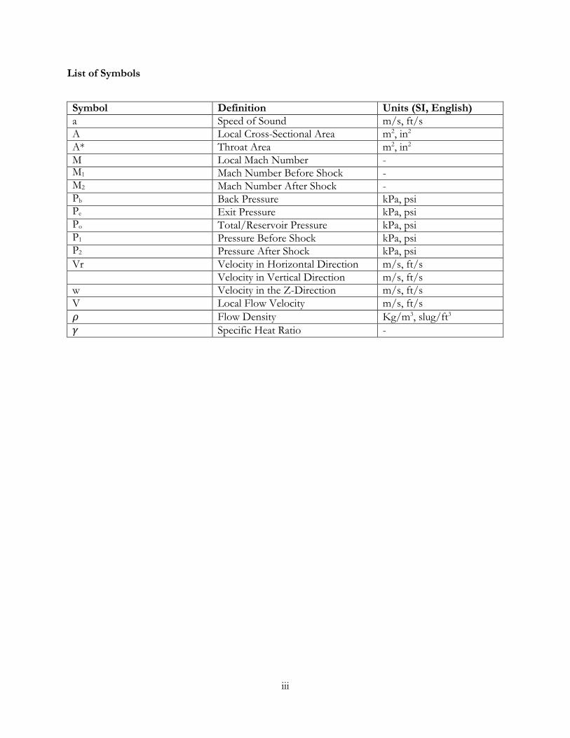
iii
List of Symbols
Symbol Definition Units (SI, English) a Speed of Sound m/s, ft/s A Local Cross-Sectional Area m2, in2
A* Throat Area m2, in2
M Local Mach Number - M1 Mach Number Before Shock - M2 Mach Number After Shock - Pb Back Pressure kPa, psi Pe Exit Pressure kPa, psi Po Total/Reservoir Pressure kPa, psi P1 Pressure Before Shock kPa, psi P2 Pressure After Shock kPa, psi Vr Velocity in Horizontal Direction m/s, ft/s
Velocity in Vertical Direction m/s, ft/s w Velocity in the Z-Direction m/s, ft/s V Local Flow Velocity m/s, ft/s 𝜌𝜌 Flow Density Kg/m3, slug/ft3
𝛾𝛾 Specific Heat Ratio -
1
1 Introduction
1.1 Background
Although World War II officially ended in 1945, there was a great deal of geopolitical tension. This
instability amongst the great powers of the world led to the Cold War. Of the world’s great powers,
the Cold War’s core was rooted in a competition of technological superiority between the United
States and the Soviet Union. One of the key categories in this competition was space exploration and
the space race. This caused the need for high speed launch and re-entry vehicles.
Today, there is a similar space race. However, unlike the Cold War when the race was between
government funded international powers, it is now between private companies such as Blue Origin,
SpaceX, Orbital Sciences, and Virgin Galactic [1-3]. In order to move forward with a design, various
subscale tests must be done. These subscale tests include CFD simulations and wind tunnel testing.
While CFD is a powerful tool, results are not always concrete as it requires a high level of user input.
Wind tunnels on the other hand, provide a controlled testing environment which results in more
realistic subscale model testing to determine aerodynamic characteristics. Engineers then use the
subscale data to predict how the full-scale model would perform during its mission.
1.1.1 Introduction to Supersonic Wind Tunnels
A supersonic wind tunnel is a facility designed to produce supersonic flows through a test section
where experimental tests are conducted and data is collected. Typically, these experiments are done
to analyze the flow behavior over subscale models for aircraft and spacecraft. Subscale testing allows
engineers to iterate their design before committing funds to a full-scale model.
Two common supersonic wind tunnel configurations include blowdown and suction wind tunnels.
Blowdown wind tunnels utilize high pressures upstream of the test section which allows the flow to

2
accelerate to the desired Mach number through the nozzle. The wind tunnel currently being designed
at SJSU is a blow down wind tunnel.
Supersonic wind tunnels consist of five major components. These components are the high-pressure
reservoir, plenum, nozzle, test section, and diffuser. Once the wind tunnel runs, air flows from the
high-pressure tanks to the plenum. The plenum is used to slow down the flow to subsonic speeds
and to accommodate for the pressure variation in the flow. The air accelerates through the nozzle
and enters into the test section where the experiment is conducted and data is collected. Finally, the
diffuser reduces the speed and pressure of the air before it exits the wind tunnel. For the nozzle to
produce a shock-free flow at the desired Mach number, the inlet-to-exit pressure ratio must maintain
a certain ratio and needs to be regulated. Since the diffuser reduces the exit pressure, the required
inlet pressure is greatly reduced [4-6]. The remainder of this report focuses on the nozzle section.
Figure 1.2.1 is a sketch of the five components highlighted above.
Figure 1.2.1 – Supersonic Wind Tunnel Schematic
1.1.2 de Laval Nozzle (Convergent-Divergent Nozzle)
A de Laval nozzle, also known as a convergent-divergent (CD) nozzle is composed of three sections:
a converging section, throat, and a diverging section. The flow is subsonic (M<1) as it exits the plenum
and enters the converging section of the nozzle. Once the flow is in the converging section of the

3
nozzle, the flow accelerates due to decreasing area. This is justified via conservation of mass flow
rate. The flow continues downstream to the throat, where the cross-sectional area is smallest. At the
throat of a correctly designed nozzle, the flow is choked (M=1). In order for nozzle to reach sonic
conditions at the throat, the inlet cross-sectional area to throat area ratio must be a certain value.
Additionally, the inlet-to-exit pressure ratio must be a certain value that corresponds to the free stream
Mach number. Finally, the flow enters the diverging section where it becomes supersonic (M>1) and
accelerates to the design Mach number. Like the converging section, the diverging section is also
driven by the area and pressure ratios [7-9].
At any given moment while the wind tunnel is running, the exit pressure (Pe), may not be equal to the
back pressure (Pb). Nature corrects this discontinuity through expansion waves and oblique shocks.
Thus, one of following scenarios may occur.
• (Pe<Pb): Nozzle is overexpanded, oblique shocks form.
• (Pe=Pb): Nozzle is perfectly expanded.
• (Pe>Pb): Nozzle is under-expanded, expansion waves form.
While a perfectly expanded nozzle is the ideal case, wind tunnels may operate when the nozzle is
overexpanded. In the absence of a diffuser, an overexpanded nozzle may still be used to perform
experiments and collect data [10].
1.1.3 Two-Dimensional Nozzle
A two-dimensional (2D) nozzle is a nozzle that has a rectangular cross section. Traditionally, wind
tunnels utilize a 2D nozzle due to the relatively ease of design and manufacturability.

4
Although 2D nozzles are commonly used in wind tunnel facilities, a major drawback is the uncertainty
in the flow caused by the formation of vortices in the corners of the nozzle. While the flow remains
uniform within the inviscid core, this uncertainty reduces the size of the area [11].
1.1.4 Axisymmetric Nozzle (Three-Dimensional Nozzle)
An axisymmetric nozzle is a three-dimensional (3D) nozzle. Unlike a 2D nozzle, an axisymmetric
nozzle does not have corners which negates the formation of vortices, resulting in a higher quality
flow. Although axisymmetric nozzles are not as commonly used in wind tunnel facilities, they are
commonly used in rocket propulsion applications.
The unique design of an axisymmetric nozzle for a wind tunnel requires involved mathematics as there
is a limited amount of historical data and past research documentation. [12].
1.2 Motivation
1.2.1 Summary of References
Anderson’s Modern Compressible Flow, illustrates the differences between the design of a 2D nozzle via
method of characteristics (MOC) and the design of an axisymmetric nozzle via MOC. These
differences are summarized below.
• The compatibility equations for the design of an axisymmetric nozzle are differential equations
while the 2D version’s compatibility equations are algebraic.
• The (𝜃𝜃 + 𝑣𝑣) quantities along the C+ and C- characteristics for the axisymmetric MOC varies
with spatial location while the (𝜃𝜃 + 𝑣𝑣) quantities remain constant along the C+ and C-
characteristics for the 2D MOC.
Anderson also states that the axisymmetric MOC must be solved with finite differences. It is also
states that such techniques are beyond the scope of the book [12].

5
Rakich’s NASA technical note reviews the MOC for 3D supersonic flow. Two methods are discussed:
the reference plane method and bicharacteristic method. Additionally, Rakich highlights principle
complications that come with the 3D MOC. These complications are summarized below.
• The presence of “cross-derivatives” not along a characteristic in the compatibility equations.
• Interpolation is necessary.
Rakich also explains that these complications are reduced by implementing a reference plane method
with a uniform, predefined grid. He also ensures that using this method will produce second-order
accuracy. Rakich presents results for flow around inclined circular cones using the methods discussed.
The report did not include the implantation of the methods discussed to design an axisymmetric
nozzle [13].
Zucrow and Hoffman’s Gas Dynamics investigates the principle theory behind the MOC. It also
includes 2D and axisymmetric applications for the MOC. Examples of numerical methods are also
presented. Unfortunately, there was no content covering the application of the MOC for the design
of an axisymmetric nozzle [14].
McCabe’s report on supersonic nozzle design highlights the design method for supersonic nozzles.
The design includes the nozzle’s contour to produce a shock-free flow. The report also demonstrates
how to calculate the flow inside the nozzle’s throat. This report did not include any axisymmetric
nozzle design [15].
Hartfield and Burkhalter’s conference paper provided a design approach for axisymmetric nozzles via
MOC. The conference paper derives the 3D MOC characteristics and compatibility equations from
fundamental principles. This procedure is outlined in a concise, step-by-step method. However, the
report does not show the procedure used for the implantation of the numerical methods used to

6
complete the nozzle design via axisymmetric MOC. To complete the design, Hartfield and Burkhalter
use a computer solver. Essentially, this report provides an explanation to the fundamental principles
behind the nozzle design tool that they used. It did not cover the implantation of these principles
while the software ran [12].
1.2.2 Importance of Work – Closing the Gap
Although the references reviewed above provide a solid foundation for the MOC, numerical methods,
axisymmetric flows, and 2D nozzle design, none of these references provide a complete step-by-step
procedure for the design of an axisymmetric nozzle. Since there are supersonic aircraft, rockets,
missiles, and a few supersonic wind tunnels that utilize axisymmetric nozzles, a method for
axisymmetric nozzle design must already exit. However, the design process is not easily accessible to
the public. The purpose of this project is to provide engineers and designers an easily accessible
procedure for the design of an axisymmetric supersonic nozzle via MOC. This will be done by
implementing numerical methods to the MOC for axisymmetric nozzle design.
1.3 Project Proposal
1.3.1 Project Goal
The purpose of this report is to present a method to design a supersonic, axisymmetric nozzle for the
use in a wind tunnel facility. An example of a nozzle design will also be presented and verified with
CFD to justify the design method.
1.3.2 Design Methodology
Preliminary analysis on quasi 1-D flow, expansion waves, oblique shocks, supersonic nozzle design
and axisymmetric flows must be done before the design process. The methodology used for the design
of the axisymmetric nozzle is the following:
1. Analysis on quasi 1-D flow, nozzle and axisymmetric nozzle design and axisymmetric flows.

7
2. Develop a Matlab code that performs a quasi 1-D study to size the nozzle’s exit-to-throat area
ratio.
3. Develop a Matlab code that executes an axisymmetric Method of Characteristics to avoid
shocks in the nozzle as an initial design of the nozzle’s contour.
4. Summarize method used for future nozzle designer’s reference.
5. Validate nozzle contour using historical data
6. Perform a sensitivity analysis on key parameters
After the nozzle design is finalized, it will be machined and integrated into the supersonic wind tunnel
at SJSU where it will be used for re-entry vehicle research.

8
2 Reduced Order Model
A reduced order model is used as a preliminary design tool to give a prediction of the nozzle’s
performance in the wind tunnel. A quasi-one-dimensional Matlab program was written to provide a
visual representation of the flow conditions. The Matlab program intakes the nozzle geometry and
determines the Mach number, temperature ratio, pressure ratio, and any shocks that may occur based
off flow conditions. The values are presented graphically while the flow passes through the nozzle.
These values are necessary to determine the design envelope for the wind tunnel configuration.
Regardless, this reduced order model is not useful for the design of the nozzle’s contour to ensure a
shock-free flow.
2.1 Quasi-One-Dimensional Flow
A quasi-one-dimensional flow (quasi-1D flow) is a flow in which the flow parameters only vary along
one direction. A quasi-1D flow analysis yields a top-level design for a nozzle. Mainly, this analysis
calculates rough pressure ratios and expansion ratio for the design Mach number. Figure 2.1.1
illustrates a quasi-1D flow through a duct.
Figure 2.1.1 – Quasi-one-dimensional flow in a duct [17]

9
2.1.1 Isentropic Flow
For the reduced order model, the core flow is assumed to be isentropic. An isentropic flow is the
ideal type of flow as it is both adiabatic, meaning no heat addition and inviscid. This assumption may
be justified by the following.
• Heat transfer effects between the flow and the nozzle walls are minimal due to short run
times of the high-speed flow.
• Reynolds number of the core is much higher than the Reynolds number near the nozzle walls.
o Due to the characteristic length to the nozzle core being greater.
During experiments, subscale models will be placed in the center of the test section where it will only
be under the influence of the isentropic core flow. Figure 2.1.2 illustrates the geometry of a
predetermined CD nozzle. This nozzle geometry was used for the quasi-1D calculations and is
designed to generate a Mach 3 flow. Based off plenum conditions, a Mach 3 nozzle was selected due
to its optimal run time and usable test area of an overexpanded nozzle [18].
Figure 2.1.2 – Geometry of Predetermined Nozzle.

10
With the geometry of the nozzle known, the area-Mach relationship presented below is used to
determine the Mach number at each location along the nozzle’s length. The Matlab code forces the
nozzle to choke at the throat and assumes that the specific heat ratio (𝛾𝛾) is 1.4 (standard for air).
𝐴𝐴 2 1 2
𝛾𝛾−1
(𝛾𝛾+1)/(𝛾𝛾−1) 2
( ∗) = 2 [( ) (1 + 𝑀𝑀 )] (2.1) 𝐴𝐴 𝑀𝑀 𝛾𝛾+1 2
The area-Mach relationship yields a subsonic and supersonic value for each area ratio. Although the
flow is accelerating through the converging section it remains subsonic until it reaches the throat
where it chokes. After the throat, the flow enters the diverging section where the pressure ratio
between the backpressure and plenum drives the flow to either accelerate to supersonic or decelerate
to subsonic. The equation that describes this relationship is shown below.
− 𝛾𝛾
𝑃𝑃
𝑃𝑃𝑜𝑜 = (1 + 𝛾𝛾−1 𝑀𝑀2)
2 𝛾𝛾−1 (2.2)
Finally, there is one last scenario: a fully subsonic solution. Figure 2.1.3 below illustrates the three
possible scenarios for the Mach 3 nozzle shown in Figure 2.1.2.
Figure 2.1.3 – Pressure Ratio Driving the Mach Number Throughout the Nozzle.

11
]𝑀𝑀
2.1.2 Non-Isentropic Flow
Non-isentropic flows occur when there is a change in entropy within the flow. Nature accommodates
for this sharp change with shockwaves. Shockwaves increase the pressure to match the back pressure
to be continuous. There are two types of shockwaves that may form: normal or oblique shocks.
Normal shocks occur normal to the flow and are the strongest shock wave. Oblique shocks are weaker
and are angled to the flow direction.
2.1.2.1 Normal Shocks
Across a normal shock, the total pressure suddenly decreases, the pressure ratio increases, and the
flow becomes subsonic. Equation 2.3 and 2.4 describes the Mach number relationship and pressure
ratio across a normal shock.
1+[𝛾𝛾−1 2 𝑀𝑀 = √ 2 1
(2.3) 2 𝛾𝛾𝑀𝑀2−(𝛾𝛾−1)
1 2
𝑃𝑃𝑜𝑜 = 1 + 2𝛾𝛾 (𝑀𝑀2 − 1) (2.4)
𝑃𝑃𝑏𝑏 𝛾𝛾+1 1
By manipulating equations 2.2 through 2.4, a ratio between the plenum pressure and the back pressure
(Po/Pb) is found. This ratio is used to determine if a normal shock will occur within the nozzle and if
a normal shock occurs at the nozzle exit.
2.1.2.2 Oblique Shocks
Oblique shocks occur when the nozzle is overexpanded. This is when Po/Pb is higher than the value
required for a normal shock to occur at the nozzle exit but less than the value required for an isentropic
flow. Oblique shocks allow the pressure to increase to match the back pressure. Oblique shocks also
decrease the Mach number. However, these changes in pressure and Mach number are not as drastic
compared to the normal shock. Unlike the normal shock, oblique shocks occur at an angle 𝛽𝛽, which

12
often allow the flow to remain supersonic. If the tunnel were to run overexpanded without a test
section, oblique shock calculations are necessary to determine the usable area behind the nozzle exit.
2.1.3 Expansion Waves
Expansion waves occur when the nozzle is Underexpanded. This is when Po/Pb is higher than the
value required for the perfectly expanded nozzle. Expansion waves accelerate the flow, increasing the
Mach number.
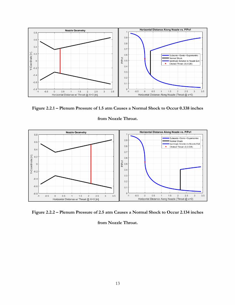
2.2 The Matlab Code
The Matlab code uses the isentropic and shock relationships to determine the required plenum
pressure to have a perfectly expanded flow and the required plenum pressure to have a normal shock
at the exit of the nozzle. Additionally, the Matlab code prompts the user to input a plenum pressure
and shows the user if a normal shock, oblique shocks, or expansion waves occur based off the plenum
pressure. If a normal shock occurs within the diverging section, the code finds the location of the
shock. If the nozzle is overexpanded, the code will determine where the oblique shocks converge
behind the nozzle exit. Finally, if the nozzle is Underexpanded, the code will determine what Mach
number the flow will expand to. Examples of the non-isentropic scenarios for the same Mach 3
nozzle are presented in Figures 2.2.1 through 2.2.5 below. For the same nozzle, the Matlab code
determined that a plenum pressure of 36.7 will yield a perfectly expanded nozzle and for a normal
shock to occur at the nozzle exit the plenum pressure must be 3.55 atm.
13
Figure 2.2.1 – Plenum Pressure of 1.5 atm Causes a Normal Shock to Occur 0.338 inches
from Nozzle Throat.
Figure 2.2.2 – Plenum Pressure of 2.5 atm Causes a Normal Shock to Occur 2.134 inches
from Nozzle Throat.

14
Figure 2.2.3 – Plenum Pressure of 3.55 atm Causes a Normal Shock to Occur at Nozzle Exit.
Figure 2.2.4 – Plenum Pressure of 4.5 atm Causes Oblique Shocks to Occur. The Shocks
Converge 0.838 inches from the Nozzle Exit.

15
Figure 2.2.5 – Plenum Pressure of 30 atm Causes Oblique Shocks to Occur. The Shocks
Converge 4.20 inches from the Nozzle Exit.

16
3 Nozzle Contour Design Method
While the importance of the reduced order model covered in the previous chapter cannot be
overlooked, the quasi-1D flow analysis is not useful for the design of the nozzle’s contour. It is
necessary that nozzle’s contour is designed in a fashion that allows for a shock-free expansion. To do
this, a modified version of the 2D method of characteristics is used to produce the desired supersonic,
axisymmetric flow. For the remainder of this report this method will be referred to as the
axisymmetric MOC.
3.1 2D Method of Characteristics
This section highlights the 2D MOC procedure used to design a Mach 3, 2D nozzle contour. The 2D
MOC provides a solid foundation to the visual understanding of the 3D method to be developed in
chapter 4.
A 2D nozzle is designed via MOC. The 2D MOC is derived from the governing equation for a 2D,
steady, adiabatic, irrotational flow.
(1 − 1 𝛿𝛿𝛿𝛿 2
𝛿𝛿2𝛿𝛿
1 𝛿𝛿𝛿𝛿 2
𝛿𝛿2𝛿𝛿
2 𝛿𝛿𝛿𝛿 𝛿𝛿𝛿𝛿 𝛿𝛿2𝛿𝛿
𝑎𝑎2 (𝛿𝛿𝛿𝛿 ) ) 𝛿𝛿𝛿𝛿2 + (1 − 𝑎𝑎2 (𝛿𝛿𝛿𝛿 ) )
𝛿𝛿𝛿𝛿2 − 𝑎𝑎2 𝛿𝛿𝛿𝛿 𝛿𝛿𝛿𝛿 𝛿𝛿𝛿𝛿𝛿𝛿𝛿𝛿
= 0 (3.1)
Substituting in velocity potential terms and differentiating yields equations 3.2 through 3.4.
(1 − 𝑢𝑢2) 𝛿𝛿
2𝛿𝛿 + (1 − 𝑣𝑣2) 𝛿𝛿
2𝛿𝛿 − 2𝑢𝑢𝑣𝑣 𝛿𝛿2𝛿𝛿 = 0 (3.2)
𝑎𝑎2 𝛿𝛿𝛿𝛿2 𝑎𝑎2 𝛿𝛿𝛿𝛿2 𝑎𝑎2 𝛿𝛿𝛿𝛿𝛿𝛿𝛿𝛿
𝑑𝑑𝑢𝑢 = 𝛿𝛿2𝛿𝛿 𝑑𝑑𝛿𝛿 + 𝛿𝛿2𝛿𝛿 𝑑𝑑𝛿𝛿 (3.3)
𝛿𝛿𝛿𝛿2 𝛿𝛿𝛿𝛿𝛿𝛿𝛿𝛿
𝑑𝑑𝑣𝑣 = 𝛿𝛿2𝛿𝛿 𝑑𝑑𝛿𝛿 + 𝛿𝛿2𝛿𝛿 𝑑𝑑𝛿𝛿 (3.4)
𝛿𝛿𝛿𝛿𝛿𝛿𝛿𝛿 𝛿𝛿𝛿𝛿2
The step by step derivation of equations 3.2 through 3.4 can be found in reference 11. These equations
can be used as a system of equations to solve for 𝛿𝛿2𝛿𝛿
𝛿𝛿𝛿𝛿𝛿𝛿𝛿𝛿
using Cramer’s rule shown in equation 3.5.

17
2
− √
2
2
𝑢𝑢2 𝑣𝑣2
𝛿𝛿2𝛿𝛿 =
1−𝑎𝑎2 0 1−𝑎𝑎2 | 𝑑𝑑𝛿𝛿 𝑑𝑑𝑢𝑢 0 |
0 𝑑𝑑𝑣𝑣 𝑑𝑑𝛿𝛿
(3.5)
𝛿𝛿𝛿𝛿𝛿𝛿𝛿𝛿 1−𝑢𝑢2
| 𝑎𝑎 2𝑢𝑢𝑣𝑣 𝑎𝑎2
1−𝑣𝑣2
𝑎𝑎2|
𝑑𝑑𝛿𝛿 𝑑𝑑𝑢𝑢 0 0 𝑑𝑑𝑣𝑣 𝑑𝑑𝛿𝛿
Where 𝛿𝛿
2𝛿𝛿
𝛿𝛿𝛿𝛿𝛿𝛿𝛿𝛿 is indeterminate along the characteristic line when the numerator and denominator is set
to zero in equation 3.5. Furthermore, the direction of the characteristic lines is found by setting the
denominator to zero and solving for 𝑑𝑑𝛿𝛿. This yields equation 3.6 below. 𝑑𝑑𝛿𝛿
𝑢𝑢𝑣𝑣 𝑢𝑢2+𝑣𝑣2 ± [ ]−1 𝑑𝑑𝛿𝛿 ( ) =
𝑑𝑑𝛿𝛿 𝑐𝑐ℎ𝑎𝑎𝑎𝑎
𝑎𝑎2 𝑎𝑎2 𝑢𝑢2
1−(𝑎𝑎2) (3.6)
Equation 3.6 is further simplified by substituting the speed of sound with the local Mach angle u with
Vcos𝜃𝜃 and v with Vsin𝜃𝜃. This relationship is shown below in equation 3.7.
𝑑𝑑𝛿𝛿
( 𝑑𝑑𝛿𝛿
)
𝑐𝑐ℎ𝑎𝑎𝑎𝑎
= tan(𝜃𝜃 ∓ 𝜇𝜇) (3.7)
Equation 3.7 shows that any given point within the nozzle, can be defined by the intersection of two
characteristic lines. These characteristic lines are referred to as a left-running (𝐶𝐶+) characteristic and
a right-running (𝐶𝐶−) characteristic. Once the characteristic lines are found, the compatibility equations
that hold true along the characteristic lines are found by setting the numerator to zero. This is shown
below in equation 3.8.
𝑑𝑑𝑣𝑣 = −
(1−𝑢𝑢2)
𝑎𝑎
𝑑𝑑𝛿𝛿
(3.8)
𝑑𝑑𝑢𝑢 (1−𝑣𝑣2 ) 𝑑𝑑𝛿𝛿
𝑎𝑎
Substituting equation 3.6 into 3.8 yields equation 3.9 shown below.
−

18
2
2
𝑑𝑑𝑣𝑣 = 𝑢𝑢𝑣𝑣 ∓
√𝑢𝑢2+𝑣𝑣2−1
𝑎𝑎
(3.9) 𝑑𝑑𝑢𝑢 𝑎𝑎2 (1−𝑣𝑣2
) 𝑎𝑎
After substituting u Vcos𝜃𝜃 and v with Vsin𝜃𝜃 and algebraic manipulation, equation 3.9 becomes
equations 3.10. Additionally, integrating equation 3.9 yields the Prandtl-Meyer function applied as an
algebraic expression shown in equation 3.11 and 3.12.
𝑑𝑑𝜃𝜃 = ∓√𝑀𝑀2 − 1 𝑑𝑑𝑑𝑑
𝑑𝑑
(3.10)
𝜃𝜃 + 𝜈𝜈(𝑀𝑀) = 𝐾𝐾− (3.11)
𝜃𝜃 − 𝜈𝜈(𝑀𝑀) = 𝐾𝐾+ (3.12)
Equations 3.2 and 3.3 state that the 𝐾𝐾− and 𝐾𝐾+ values along any 𝐶𝐶−and 𝐶𝐶+characteristic is constant.
Hence, once the 𝐾𝐾− or 𝐾𝐾+value is known at any given point, that value will remain constant along the
respective characteristic line.
3.1.1 2D Method of Characteristics Implementation
This section contains an example of the process used to design a minimum length, 2D, Mach 3 nozzle.
For this example, seven characteristic lines are used. It should be noted that there are an infinite
number of characteristic lines and that the use of more characteristic lines correlates to higher
accuracy. Regardless, the purpose of this section is to show the implantation of the 2D MOC, thus
the goal of this example is to design a contour that is within a ten percent error margin of the quasi-
1D calculations.
The nozzle throat height is a preset value of 0.9445 inches. Thus, from the centerline, the distance is
0.472 inches. This value was selected based off constraints set by optimizing plenum pressure, exit
area, and a constant depth of 4 inches throughout the expansion section. The seven characteristic lines
start at the throat to form a simple expansion. These characteristics extend to and reflect off the

19
nozzle centerline. This configuration yields a total of 35 points. Figure 3.1.1 is schematic showing
the characteristic lines.
Figure 3.1.1: Schematic of Seven Characteristic Lines [11]
The Prandtl Meyer angle (𝑣𝑣) that corresponds to Mach 3 is 49.76 degrees. Half of this value yields
the highest 𝜃𝜃 value for the nozzle contour. This angle is formed with the line between points a and 8
with the horizontal. Once this angle is found, the angles of points one through nine are found by a
constant change in 𝜃𝜃. After these initial steps are done, the properties of the remaining points are
found using equations 3.1 through 3.3. Table 3.1 summarizes the properties of each point within the
web of characteristic lines.

20
Table 3.1: Seven Line MOC for a Mach 3 Nozzle. Wall points are highlighted.
Point # k- = Ꝋ+ν k+ = Ꝋ-ν Ꝋ = 1/2(k-+k+) ν= 1/2(k--k+) M μ Ꝋ+μ & Wall Inlincation Ꝋ-μ x y a 0.004 0 0.002 0.002 1.001 87.215 24.88 0 0.472 1 1.76 0 0.88 0.88 1.0749 68.4827 69.3627 -68.4827 0.18609 0 2 9.76 0 4.88 4.88 1.2519 53.0136 57.8936 -53.0136 0.24256 0.14995 3 17.76 0 8.88 8.88 1.3963 45.7406 54.6206 -45.7406 0.27048 0.19444 4 25.76 0 12.88 12.88 1.533 40.7151 53.5951 -40.7151 0.29022 0.22224 5 33.76 0 16.88 16.88 1.6684 36.8256 53.7056 -36.8256 0.3056 0.24314 6 41.76 0 20.88 20.88 1.8054 33.6354 54.5154 -33.6354 0.31823 0.26029 7 49.76 0 24.88 24.88 1.946 30.9224 55.8024 -30.9224 0.32876 0.27507 8 49.76 0 24.88 24.88 1.946 30.9224 22.44 0.67545 0.78525 9 9.76 -9.76 0 9.76 1.4267 44.4999 44.4999 -44.4999 0.39515 0
10 17.76 -9.76 4 13.76 1.5628 39.7824 43.7824 -35.7824 0.45654 0.06033 11 25.76 -9.76 8 17.76 1.6983 36.0736 44.0736 -28.0736 0.50561 0.10736 12 33.76 -9.76 12 21.76 1.4954 33.0031 45.0031 -21.0031 0.54926 0.14961 13 41.76 -9.76 16 25.76 1.9776 30.3756 46.3756 -14.3756 0.59022 0.19058 14 49.76 -9.76 20 29.76 2.1249 28.0745 48.0745 -8.0745 0.63001 0.23233 15 49.76 -9.76 20 29.76 2.1249 28.0745 18 1.39251 1.08138 16 17.76 -17.76 0 17.76 1.4954 36.0736 36.0736 -36.0736 0.53936 0 17 25.76 -17.76 4 21.76 1.8359 33.0031 37.0031 -29.0031 0.60846 0.05034 18 33.76 -17.76 8 25.76 1.9776 30.3756 38.3756 -22.3756 0.67273 0.09878 19 41.76 -17.76 12 29.76 2.1249 28.0745 40.0745 -16.0745 0.73571 0.14865 20 49.76 -17.76 16 33.76 2.2792 26.0239 42.0239 -10.0239 0.79955 0.20236 21 49.76 -17.76 16 33.76 2.2792 26.0239 14 1.99064 1.27573 22 25.76 -25.76 0 25.76 1.9776 30.3756 30.3756 -30.3756 0.69435 0 23 33.76 -25.76 4 29.76 2.1249 28.0745 32.0745 -24.0745 0.78063 0.05057 24 41.76 -25.76 8 33.76 2.2792 26.0239 34.0239 -18.0239 0.86829 0.10551 25 49.76 -25.76 12 37.76 2.4422 24.1714 36.1714 -12.1714 0.96037 0.16767 26 49.76 -25.76 12 37.76 2.4422 24.1714 10 2.72706 1.45934 27 33.76 -33.76 0 33.76 2.2792 26.0239 26.0239 -26.0239 0.88421 0 28 41.76 -33.76 4 37.76 2.4422 24.1714 28.1714 -24.1714 0.98918 0.05125 29 49.76 -33.76 8 41.76 2.6154 22.4794 30.4794 -22.4794 1.09926 0.1102 30 49.76 -33.76 8 41.76 2.6154 22.4794 6 3.67572 1.62661 31 41.76 -41.76 0 41.76 2.6154 22.4794 22.4794 -22.4794 1.11305 0 32 49.76 -41.76 4 45.76 2.8007 20.9195 24.9195 -16.9195 1.2607 0.0611 33 49.76 -41.76 4 45.76 2.8007 20.9195 2 4.9094 1.75628 34 49.76 -49.76 0 49.76 3 19.47 19.47 -19.47 1.43351 0 35 49.76 -49.76 0 49.76 3 19.47 0 6.56487 1.81409
Execution of the 2D MOC for a Mach 3 nozzle with seven characteristic lines provided decent results.
The quasi-1D expansion ratio was calculated to be 4.235 while the 2D MOC yielded a value of 3.843.
The percent error for this design is 9.24% which is within the ten percent margin desired to justify the
method. The design of this nozzle is shown in figure 3.1.2. This figure was produced in Solidworks
by following the characteristic web and plotting each line at the specified angles listed in Table 3.1,
columns eight and nine (𝜃𝜃 + 𝜇𝜇) 𝑎𝑎𝑎𝑎𝑑𝑑 (𝜃𝜃 − 𝜇𝜇).

21
Figure 3.1.2: Seven Line MOC for a Mach 3 Nozzle.
3.2 Axisymmetric Method of Characteristics - Derivation
The axisymmetric method of characteristics is an iterative method used for designing an axisymmetric
nozzle. The nozzle contour is designed by locating and solving for characteristic lines. Although this
method is similar to the 2D MOC, slight differences in the compatibility equations cause for an
iterative process. Additionally, the axisymmetric MOC requires multiple assumptions and inputs to
yield a successful nozzle design covered in section four. To justify convergence, the expansion ratio
is iterated over and checked against the quasi-1D value.
𝜕𝜕(𝜌𝜌𝑢𝑢) + 𝜕𝜕(𝜌𝜌𝑣𝑣) + 1 𝜕𝜕(𝜌𝜌𝜌𝜌) + 𝜌𝜌𝑣𝑣 = 0 (3.13) 𝜕𝜕𝛿𝛿 𝜕𝜕𝑎𝑎 𝑎𝑎 𝜕𝜕∅ 𝑎𝑎
Accounting for steady, inviscid, axisymmetric, irrotational, flow, equation 3.13 yields
(1 − 𝑢𝑢2) 𝜕𝜕𝑢𝑢 − 2 𝑢𝑢𝑣𝑣 𝜕𝜕𝑣𝑣 + (1 − 𝑣𝑣
2) 𝜕𝜕𝑣𝑣 = − 𝑣𝑣
(3.14)
𝑎𝑎2 𝜕𝜕𝛿𝛿 𝑎𝑎2 𝜕𝜕𝛿𝛿 𝑎𝑎2 𝜕𝜕𝑎𝑎 𝑎𝑎
𝑑𝑑𝑢𝑢 = 𝜕𝜕𝑢𝑢 𝑑𝑑𝛿𝛿 + 𝜕𝜕𝑣𝑣 𝑑𝑑𝑎𝑎 (3.15)
𝜕𝜕𝛿𝛿 𝜕𝜕𝛿𝛿
𝑑𝑑𝑣𝑣 = 𝜕𝜕𝑣𝑣 𝑑𝑑𝛿𝛿 + 𝜕𝜕𝑣𝑣 𝑑𝑑𝑎𝑎 (3.16)
𝜕𝜕𝛿𝛿 𝜕𝜕𝑎𝑎

22
− √
2
2 2
The step by step derivation of equations 3.2 through 3.4 can be found in reference 11. These equations
can be used as a system of equations to solve for 𝜕𝜕𝑣𝑣 using Cramer’s rule shown in equation 3.15. 𝜕𝜕𝛿𝛿
𝑢𝑢2 𝑣𝑣 𝑣𝑣2
𝜕𝜕𝑣𝑣 =
1−𝑎𝑎2 −𝑎𝑎 1−𝑎𝑎2 | 𝑑𝑑𝛿𝛿 𝑑𝑑𝑢𝑢 0 |
0 𝑑𝑑𝑣𝑣 𝑑𝑑𝑎𝑎
(3.15)
𝜕𝜕𝛿𝛿 1−𝑢𝑢2
−2𝑢𝑢𝑣𝑣 1−𝑣𝑣2
| 𝑎𝑎2 𝑎𝑎2 𝑎𝑎2| 𝑑𝑑𝛿𝛿 𝑑𝑑𝑎𝑎 0 0 𝑑𝑑𝛿𝛿 𝑑𝑑𝑎𝑎
Similar to the 2D MOC, the direction of the characteristic lines is found by setting the denominator
to zero and solving for 𝑑𝑑𝑎𝑎. This yields equation 3.16 below.
𝑑𝑑𝛿𝛿
𝑢𝑢𝑣𝑣 𝑢𝑢2+𝑣𝑣2 ± [ ]−1
(𝑑𝑑𝑎𝑎) = 𝑎𝑎2 𝑎𝑎2 𝑢𝑢2 (3.16)
𝑑𝑑𝛿𝛿 𝑐𝑐ℎ𝑎𝑎𝑎𝑎 1−(𝑎𝑎2)
Equation 3.6 is further simplified by substituting the speed of sound with the local Mach angle u with
Vcos𝜃𝜃 and v with Vsin𝜃𝜃. This simplification shows that for an axisymmetric flow, the characteristic
lines are Mach lines and that the left-running C+ characteristic and right-running C- characteristic are
the same as the 2D case. This relationship is shown below in equation 3.17.
(𝑑𝑑𝑎𝑎) = tan(𝜃𝜃 ∓ 𝜇𝜇) (3.17) 𝑑𝑑𝛿𝛿 𝑐𝑐ℎ𝑎𝑎𝑎𝑎
Once the characteristic lines are found, the compatibility equations that hold true along the
characteristic lines are found by setting the numerator to zero. This is shown below in equation 3.18.
𝑑𝑑𝑣𝑣 = −
(1−𝑢𝑢2)
𝑎𝑎 𝑑𝑑𝑎𝑎 −
𝑣𝑣 𝑑𝑑𝑎𝑎 𝑎𝑎𝑑𝑑𝑢𝑢
(3.18)
𝑑𝑑𝑢𝑢 (1−𝑣𝑣2 ) 𝑑𝑑𝛿𝛿
𝑎𝑎 (1−𝑣𝑣2
) 𝑎𝑎
Substituting equation 3.16 into 3.18 yields equation 3.19 shown below.

23
2
2 2
𝑑𝑑𝑣𝑣 = 𝑢𝑢𝑣𝑣 ∓
√𝑢𝑢2+𝑣𝑣2−1
𝑎𝑎 −
𝑣𝑣 𝑑𝑑𝑎𝑎 𝑎𝑎𝑑𝑑𝑢𝑢
(3.19)
𝑑𝑑𝑢𝑢 𝑎𝑎2 (1−𝑣𝑣2 )
𝑎𝑎 (1−𝑣𝑣2
) 𝑎𝑎
After substituting u Vcos𝜃𝜃 and v with Vsin𝜃𝜃 and algebraic manipulation, equation 3.19 becomes
equations 3.20 and 3.21.
𝑑𝑑(𝜃𝜃 + 𝑣𝑣) = 1
𝑑𝑑𝑎𝑎 , along a C characteristic. (3.20)
√𝑀𝑀2−1−𝑐𝑐𝑜𝑜𝑐𝑐𝜃𝜃 𝑎𝑎 -
𝑑𝑑(𝜃𝜃 − 𝑣𝑣) = −1
𝑑𝑑𝑎𝑎 , along a C characteristic. (3.21) √𝑀𝑀2−1+𝑐𝑐𝑜𝑜𝑐𝑐𝜃𝜃 𝑎𝑎 +
For an axisymmetric, irrotational flow, equations 3.20 and 3.21 are the compatibility equations.
Guentert and Neumann presented in reference 19, group the compatibility and characteristic
equations into two groups for application purposes. These two groups are presented below in
equations 3.22 through 3.25.
First group:
(𝑑𝑑𝑎𝑎) 𝑑𝑑𝛿𝛿 1
= tan(𝜃𝜃 + 𝜇𝜇) (3.22)
𝑑𝑑𝑑𝑑 − tan(𝜇𝜇) 𝑑𝑑𝜃𝜃 − tan(𝜇𝜇) sin(𝜇𝜇) sin(𝜃𝜃) 𝑑𝑑𝛿𝛿 = 0 (3.23) 𝑑𝑑 cos(𝜃𝜃+𝜇𝜇) 𝑎𝑎
Second group:
(𝑑𝑑𝑎𝑎) 𝑑𝑑𝛿𝛿 2
= tan(𝜃𝜃 − 𝜇𝜇) (3.24)
𝑑𝑑𝑑𝑑 + tan(𝜇𝜇) 𝑑𝑑𝜃𝜃 − tan(𝜇𝜇) sin(𝜇𝜇) sin(𝜃𝜃) 𝑑𝑑𝛿𝛿 = 0 (3.25) 𝑑𝑑 cos(𝜃𝜃−𝜇𝜇) 𝑎𝑎
Figure 3.1.1 offers an illustration of these two groups.

24
Figure 3.2.1 - Characteristic lines and velocity vectors of an arbitrary point in the flow.
3.3 Axisymmetric Method of Characteristics – Characteristic Point Calculation Procedure
In order to design the nozzle’s contour using the equations derived in the previous section, finite
differences and an iterative process is required. This section outlines the procedure used to locate and
calculate the flow properties at various points throughout the flow field. Figure 3.2.1 serves as visual
clarification for the procedure outlined below.

25
Figure 3.2.2 – Reference for Axisymmetric MOC Procedure
3.3.1 Step-by-step Procedure to Determine Characteristic Points
This section highlights the iterative method developed that is used to determine individual points
within the web of intersecting characteristic lines.
1. Assume properties at points A and B are known and the distance between these points is
small. Since the properties are known and small, discretization can be used transform
differential terms via finite differences. For example, given two arbitrary points 1 and 2, dr/dx
is transformed in to 𝑎𝑎2−𝑎𝑎1 . 𝛿𝛿2−𝛿𝛿1
2. Point C is the intersection of the characteristics ie: tan(𝜃𝜃𝐵𝐵 − 𝜇𝜇𝐵𝐵) and tan(𝜃𝜃𝐴𝐴 + 𝜇𝜇𝐴𝐴)
3. Solve for the location of point C (xC, rC) with finite differences.
𝑎𝑎𝐶𝐶−𝑎𝑎𝐴𝐴 = tan(𝜃𝜃 + 𝜇𝜇 ) (3.26)
𝛿𝛿𝐶𝐶−𝛿𝛿𝐴𝐴 𝐴𝐴 𝐴𝐴

26
2
𝑎𝑎𝐶𝐶−𝑎𝑎𝐵𝐵 = tan(𝜃𝜃 − 𝜇𝜇 ) (3.27) 𝛿𝛿𝐶𝐶−𝛿𝛿𝐵𝐵 𝐵𝐵 𝐵𝐵
Solving for the system of equations yield equations 3.18 and 3.19.
𝛿𝛿𝐶𝐶
= 𝑎𝑎𝐴𝐴−𝑎𝑎𝐵𝐵+𝛿𝛿𝐵𝐵 tan(𝜃𝜃𝐵𝐵−𝜇𝜇𝐵𝐵)−𝛿𝛿𝐴𝐴 tan(𝜃𝜃𝐴𝐴+𝜇𝜇𝐴𝐴) tan(𝜃𝜃𝐵𝐵−𝜇𝜇𝐵𝐵)−tan(𝜃𝜃𝐴𝐴+𝜇𝜇𝐴𝐴)
(3.28)
𝑎𝑎𝐶𝐶 = 𝑎𝑎𝐴𝐴 + (𝛿𝛿𝐶𝐶 − 𝛿𝛿𝐴𝐴) tan(𝜃𝜃𝐴𝐴 + 𝜇𝜇𝐴𝐴) (3.29)
4. Solve for VC and 𝜃𝜃𝐶𝐶 with finite differences.
𝑑𝑑𝐶𝐶−𝑑𝑑𝐴𝐴 − (𝜃𝜃 − 𝜃𝜃 )𝑐𝑐𝑎𝑎𝑎𝑎𝜇𝜇 − 𝑐𝑐𝑎𝑎𝑎𝑎𝜇𝜇𝐴𝐴𝑠𝑠𝑠𝑠𝑎𝑎𝜇𝜇𝐴𝐴𝑠𝑠𝑠𝑠𝑎𝑎𝜃𝜃𝐴𝐴 (𝛿𝛿𝐶𝐶−𝛿𝛿𝐴𝐴) = 0 (3.30)
𝑑𝑑𝐴𝐴 𝐶𝐶 𝐴𝐴 𝐴𝐴 cos(𝜃𝜃𝐴𝐴+𝜇𝜇𝐴𝐴) 𝑎𝑎𝐴𝐴
𝑑𝑑𝐶𝐶−𝑑𝑑𝐵𝐵 + (𝜃𝜃 − 𝜃𝜃 )𝑐𝑐𝑎𝑎𝑎𝑎𝜇𝜇 − 𝑐𝑐𝑎𝑎𝑎𝑎𝜇𝜇𝐵𝐵𝑠𝑠𝑠𝑠𝑎𝑎𝜇𝜇𝐵𝐵𝑠𝑠𝑠𝑠𝑎𝑎𝜃𝜃𝐵𝐵 (𝛿𝛿𝐶𝐶−𝛿𝛿𝐵𝐵) = 0 (3.31)
𝑑𝑑𝐵𝐵 𝐶𝐶 𝐵𝐵 𝐵𝐵 cos(𝜃𝜃𝐵𝐵−𝜇𝜇𝐵𝐵) 𝑎𝑎𝐵𝐵
Solving for the system of equations yields equations 3.22 and 3.23.
𝑑𝑑 = 1
[𝑐𝑐𝑜𝑜𝑐𝑐𝜇𝜇 (1 + 𝑐𝑐𝑎𝑎𝑎𝑎𝜇𝜇𝐴𝐴𝑠𝑠𝑠𝑠𝑎𝑎𝜇𝜇𝐴𝐴𝑠𝑠𝑠𝑠𝑎𝑎𝜃𝜃𝐴𝐴(𝛿𝛿𝐶𝐶−𝛿𝛿𝐴𝐴)
(1 + 𝑐𝑐𝑎𝑎𝑎𝑎𝜇𝜇𝐵𝐵𝑠𝑠𝑠𝑠𝑎𝑎𝜇𝜇𝐵𝐵𝑠𝑠𝑠𝑠𝑎𝑎𝜃𝜃𝐵𝐵(𝛿𝛿𝐶𝐶−𝛿𝛿𝐵𝐵)) + 𝜃𝜃
− 𝜃𝜃 ] (3.32)
𝐶𝐶 𝑐𝑐𝑜𝑜𝑐𝑐𝜇𝜇𝐴𝐴 𝑐𝑐𝑜𝑜𝑐𝑐𝜇𝜇𝐵𝐵 𝐴𝐴 𝑎𝑎 cos(𝜃𝜃 +𝜇𝜇 ) 𝐵𝐵 𝑎𝑎 cos(𝜃𝜃 −𝜇𝜇 ) 𝐵𝐵 𝐴𝐴 𝑑𝑑𝐴𝐴
+ 𝑑𝑑𝐵𝐵 𝐴𝐴 𝐴𝐴 𝐴𝐴 𝐵𝐵 𝐵𝐵 𝐵𝐵
𝜃𝜃 = 𝜃𝜃 + 𝑐𝑐𝑜𝑜𝑐𝑐𝜇𝜇 [𝑑𝑑𝐶𝐶−𝑑𝑑𝐴𝐴 − 𝑐𝑐𝑎𝑎𝑎𝑎𝜇𝜇𝐴𝐴𝑠𝑠𝑠𝑠𝑎𝑎𝜇𝜇𝐴𝐴𝑠𝑠𝑠𝑠𝑎𝑎𝜃𝜃𝐴𝐴(𝛿𝛿𝐶𝐶−𝛿𝛿𝐴𝐴)] (3.33) 𝐶𝐶 𝐴𝐴 𝐴𝐴 𝑑𝑑𝐴𝐴
𝑎𝑎𝐴𝐴 cos(𝜃𝜃𝐴𝐴+𝜇𝜇𝐴𝐴)
5. Calculate the speed of sound at point C to determine the Mach angle at point C.
6. Since the properties of point C were found by assuming the properties at points A and B,
a second iteration is required. This is done by averaging points A & C, and C & B. The second
iteration of point C is called C’.
7. Solve for the location of point C’ (xC’, rC’).
𝑎𝑎𝐴𝐴−𝑎𝑎𝐵𝐵+1 [tan(𝜃𝜃𝐵𝐵−𝜇𝜇𝐵𝐵)+tan(𝜃𝜃𝐶𝐶−𝜇𝜇𝐶𝐶)]𝛿𝛿𝐵𝐵−1[tan(𝜃𝜃𝐴𝐴+𝜇𝜇𝐴𝐴)+tan(𝜃𝜃𝐶𝐶+𝜇𝜇𝐶𝐶)]𝛿𝛿𝐴𝐴 𝛿𝛿′ = 2 2
(3.34)
𝐶𝐶 1[tan(𝜃𝜃𝐵𝐵−𝜇𝜇𝐵𝐵)+tan(𝜃𝜃𝐶𝐶−𝜇𝜇𝐶𝐶)−tan(𝜃𝜃𝐴𝐴+𝜇𝜇𝐴𝐴)−tan(𝜃𝜃𝐶𝐶+𝜇𝜇𝐶𝐶)]
) + 𝑐𝑐𝑜𝑜𝑐𝑐𝜇𝜇

27
𝑎𝑎′ = 𝑎𝑎 + (𝛿𝛿 − 𝛿𝛿 ) 1 [tan(𝜃𝜃
+ 𝜇𝜇 ) + tan(𝜃𝜃 + 𝜇𝜇 )] (3.35) 𝐶𝐶 𝐴𝐴 𝐶𝐶 𝐴𝐴 2 𝐴𝐴 𝐴𝐴 𝐶𝐶 𝐶𝐶
8. Solve for VC’ and 𝜃𝜃𝐶𝐶′ in a similar fashion.
𝑑𝑑′ = 1
∗
𝐶𝐶 4[(𝑑𝑑𝐴𝐴 + 𝑑𝑑𝐶𝐶)−1(𝑐𝑐𝑎𝑎𝑎𝑎𝜇𝜇𝐴𝐴 + 𝑐𝑐𝑎𝑎𝑎𝑎𝜇𝜇𝐶𝐶)−1 + (𝑑𝑑𝐵𝐵 + 𝑑𝑑𝐶𝐶)−1(𝑐𝑐𝑎𝑎𝑎𝑎𝜇𝜇𝐵𝐵 + 𝑐𝑐𝑎𝑎𝑎𝑎𝜇𝜇𝐶𝐶)−1]
𝑐𝑐𝑎𝑎𝑎𝑎𝜇𝜇𝐴𝐴𝑠𝑠𝑠𝑠𝑎𝑎𝜇𝜇𝐴𝐴𝑠𝑠𝑠𝑠𝑎𝑎𝜃𝜃𝐴𝐴+𝑐𝑐𝑎𝑎𝑎𝑎𝜇𝜇𝐶𝐶𝑠𝑠𝑠𝑠𝑎𝑎𝜇𝜇𝐶𝐶𝑠𝑠𝑠𝑠𝑎𝑎𝜃𝜃𝐶𝐶
2
𝑐𝑐𝑎𝑎𝑎𝑎𝜇𝜇𝐴𝐴+𝑐𝑐𝑎𝑎𝑎𝑎𝜇𝜇𝐶𝐶 [ 2𝑑𝑑𝐴𝐴 +
𝑑𝑑𝐴𝐴+𝑑𝑑𝐶𝐶
𝑎𝑎𝐴𝐴 cos(𝜃𝜃𝐴𝐴+𝜇𝜇𝐴𝐴) 𝑎𝑎𝐶𝐶 cos(𝜃𝜃𝐶𝐶+𝜇𝜇𝐶𝐶)
2 (𝛿𝛿𝐶𝐶 − 𝛿𝛿𝐴𝐴)]
𝑐𝑐𝑎𝑎𝑎𝑎𝜇𝜇 𝑠𝑠𝑠𝑠𝑎𝑎𝜇𝜇 𝑠𝑠𝑠𝑠𝑎𝑎𝜃𝜃 𝑐𝑐𝑎𝑎𝑎𝑎𝜇𝜇 𝑠𝑠𝑠𝑠𝑎𝑎𝜇𝜇 𝑠𝑠𝑠𝑠𝑎𝑎𝜃𝜃 (3.36) 2 2𝑑𝑑 𝐵𝐵 𝐵𝐵 𝐵𝐵+ 𝐶𝐶 𝐶𝐶 𝐶𝐶
+ { 𝑐𝑐𝑎𝑎𝑎𝑎𝜇𝜇𝐵𝐵+𝑐𝑐𝑎𝑎𝑎𝑎𝜇𝜇𝐵𝐵
[ 𝐵𝐵 + 𝑑𝑑𝐵𝐵+𝑑𝑑𝐶𝐶
𝑎𝑎𝐵𝐵 cos(𝜃𝜃𝐵𝐵−𝜇𝜇𝐵𝐵)
2 𝑎𝑎𝐶𝐶 cos(𝜃𝜃𝐶𝐶−𝜇𝜇𝐶𝐶) (𝛿𝛿𝐶𝐶 − 𝛿𝛿𝐵𝐵 )] + 𝜃𝜃𝐵𝐵 − 𝜃𝜃𝐴𝐴
}
′ 𝑐𝑐𝑎𝑎𝑎𝑎𝜇𝜇𝐴𝐴𝑠𝑠𝑠𝑠𝑎𝑎𝜇𝜇𝐴𝐴𝑠𝑠𝑠𝑠𝑎𝑎𝜃𝜃𝐴𝐴+𝑐𝑐𝑎𝑎𝑎𝑎𝜇𝜇𝐶𝐶𝑠𝑠𝑠𝑠𝑎𝑎𝜇𝜇𝐶𝐶𝑠𝑠𝑠𝑠𝑎𝑎𝜃𝜃𝐶𝐶
𝜃𝜃′ = 𝜃𝜃 + 2 [2(𝑑𝑑𝐶𝐶−𝑑𝑑𝐴𝐴) − 𝑎𝑎𝐴𝐴 cos(𝜃𝜃𝐴𝐴+𝜇𝜇𝐴𝐴) 𝑎𝑎𝐶𝐶 cos(𝜃𝜃𝐶𝐶+𝜇𝜇𝐶𝐶)
(𝛿𝛿 − 𝛿𝛿 )] (3.37) 𝐶𝐶 𝐴𝐴
𝑐𝑐𝑎𝑎𝑎𝑎𝜇𝜇𝐴𝐴+𝑐𝑐𝑎𝑎𝑎𝑎𝜇𝜇𝐶𝐶 𝑑𝑑𝐶𝐶+𝑑𝑑𝐴𝐴 2 𝐶𝐶 𝐴𝐴
9. C’ and its flow properties are now the starting point for the remaining web.

28
4 Axisymmetric Method of Characteristics Implementation
Section 3.3.1 highlights the iterative process used to determine the flow properties of a point between
two fully defined points within a web of characteristic lines. However, when applying the
axisymmetric MOC, this procedure is merely used as a tool. This section will explain the assumptions,
inputs and process developed to execute the axisymmetric MOC used to design a nozzle’s contour.
4.1 Assumptions
The following assumptions must be made correctly to use the axisymmetric MOC. These assumptions
are necessary due to the iterative nature of the procedure.
4.1.1 Initial Nozzle Length
The initial nozzle length can be described as the length along the nozzle’s axis in which the expansion
occurs. For illustrative purposes, this length can be seen in figure 3.1.1 as the distance from point b
to point 34. When using the axisymmetric MOC for the design of a nozzle, this length must initially
be assumed. This value may be iterated over if the expansion ratio calculated does not converge with
the quasi-1D value.
4.1.2 Axis-Pressure Distribution
Like the initial nozzle length, a pressure distribution also must be assumed for the design of a nozzle’s
contour via axisymmetric MOC [19]. Young reports that the following pressure distributions have
been used with success. These include a cosine, parabolic, and cubic pressure distributions. It should
be noted that the pressure distribution selection is dependent on the desired nozzle design Mach
number. Young notes that the cosine distribution is hardly useful after the nozzle throat and that
parabolic pressure distribution has proven to yield reasonable results for low Mach numbers. For
higher Mach numbers, the cubic distribution can be used by decreasing the value of q. The relations
are listed below as equations 4.1 through 4.3.

29
] 𝛿𝛿 − 𝑞𝑞𝛿𝛿 + ln(𝑝𝑝 )
Cosine: ln(𝑝𝑝) = 1 (ln(𝑝𝑝 ) − ln(𝑝𝑝 ))
𝜋𝜋𝛿𝛿
1 (ln(𝑝𝑝 ) + ln(𝑝𝑝 )) (4.1)
2 𝑐𝑐 cos ( ) + 𝑙𝑙 2
Parabolic: ln(𝑝𝑝) = 𝑙𝑙−2(𝛿𝛿 − 𝑙𝑙)2(ln(𝑝𝑝𝑐𝑐) − ln(𝑝𝑝𝑝𝑝)) + ln(𝑝𝑝𝑝𝑝) (4.2)
Cubic: ln(𝑝𝑝) = [𝑞𝑞 𝑙𝑙+2(ln(𝑝𝑝𝑐𝑐)−ln(𝑝𝑝𝑝𝑝))] 𝛿𝛿3 − [ 2𝑞𝑞𝑙𝑙+3(ln(𝑝𝑝𝑐𝑐)−ln(𝑝𝑝𝑝𝑝)) 2 (4.3)
𝑙𝑙3 𝑙𝑙2 𝑐𝑐
Where (x) varies from the nozzle’s throat through initial expansion length (l). The nozzle’s exit and
throat pressure are noted as pe and pt, respectively. Finally, the coefficient q can be used as an
additional factor that allows the cubic distribution to be manipulated further. Young provides a plot
that illustrates these pressure distributions.
Figure 4.1.1 – Young’s Pressure Distribution Plots [19]
By assuming the pressure distribution along the nozzle’s centerline, each point’s inclination (𝜃𝜃),
Prandtl-Meyer Angle (𝑣𝑣), Mach number (M), Mach angle (𝜇𝜇), and location (x,r) are known.
𝑝𝑝 𝑐𝑐 𝑝𝑝

30
4.2 Inputs
After the above assumptions are made, input values must be selected. The input values include design
Mach number, throat location, and number of characteristic lines. It must be noted that maximizing
the amount of characteristic lines used in this method will yield drastically better results. However, for
computational purposes, the user is heavily limited and must select a reasonable amount. The amount
of characteristic lines also determines the distance from the nozzle’s throat to the intersection of the
first characteristic line and the nozzle’s centerline axis.
4.3 Implementation
Based on the assumptions, and inputs the axisymmetric MOC may now be applied to design the
nozzle’s contour. Figure 3.1.1 will be used as an example for the procedure. For this example, seven
characteristic lines are used and the throat radius is the distance between points a and b. Additionally,
the points along the nozzle centerline (points 1, 9, 16, 22, 27, 31, and 34) are fully defined due to the
assumed pressure distribution. The next step is to determine the location and flow properties of points
2, 10, 17, 23, 28 and 32. This is done by following the process described in section 3.3.1. The same
process can be done to calculate each “row” that occurs below the previously calculated row. Refer
to figure 4.3.1 for a diagram showing the points used to calculate the next row of points.

31
Figure 4.3.1 – MOC Point Tree Diagram
Once the entire point tree is defined, the nozzle contour points (wall points: 8, 15, 21, 26, 30, 33 and
35) are also known. Each of these points have the same flow properties as the previous one.
However, it must be noted that the inclination for these points is the average of the previous wall
point and the point that occurs before it. For example, the inclination for point 15 will be an average
of the inclinations for points 8 and 14.
After each point’s location and flow properties are calculated, the area ratio can be found by
comparing the radius of last point to the throat radius. This value is then checked against the area
ratio that corresponds to the nozzle’s design Mach number found by quasi-1D relations. If the area
ratios do not match, iteration of the inputs and assumptions is required until the solution converges.
This extra iteration requirement further distances this 3D MOC from the 2D MOC. Executing this
process by hand can be tedious, thus a Matlab code was written to simplify this process. A colleague
of mine, Irvin Quintero has contributed to this code by aiding in cumbersome indexing problems
that were encountered.

32
4.4 Converging Section Design
Although the converging section deals with subsonic flow, the design should not be overlooked. A
nozzle designed with quasi 1D flow theory yields a sharp throat as seen in figure 2.1.2. However,
when dealing with 2D flows, a radius of curvature is required to allow the flow to become uniform at
the throat. The method used for the design of the converging section contour is Rao’s method. This
method uses circular arcs and the design throat radius to size the contour. Equations 4.4 and 4.5 yield
the coordinates for points along the converging section. Rao developed these relationships through
experimental data. Rao’s method was commonly used in the 1950’s for rocket nozzle design.
𝛿𝛿 = 1.5𝑅𝑅𝑐𝑐 ∗ cos 𝜃𝜃 (4.4)
𝑎𝑎 = 1.5𝑅𝑅𝑐𝑐 ∗ 𝑠𝑠𝑠𝑠𝑎𝑎𝜃𝜃 + 2.5𝑅𝑅𝑐𝑐 (4.5)
Where Rt is the throat radius and −130 ≤ 𝜃𝜃 ≤ −90 degrees.
4.5 Axisymmetric MOC Contour
Figure 4.5.1 is the contour produced by the axisymmetric MOC method outlined in this chapter. This
is a Mach 3 contour that utilizes a parabolic pressure distribution along initial nozzle length equal to
the throat radius. The contour is produced using 200 characteristic lines.

33
Figure 4.5.1 – Axisymmetric MOC Designed Mach 3 Nozzle Contour

34
5 Method Validation
Although CFD simulations are the ideal proof of validation for the method developed, due to deadline
restrictions and lack of CFD software knowledge, this report does not contain CFD proof. However,
Baloni designed and produced CFD simulations on a Mach 3 nozzle [21]. The CFD analysis on
Baloni’s nozzle is shown below in figure 5.1.1.
Figure 5.1.1 – Baloni’s Mach 3 Nozzle CFD Simulation
The nozzle’s geometry that Baloni designed was extrapolated via grabit.m,, a free, third-party,
Matlab function that allows for the extraction of points of an image. Baloni’s expansion section
contour was then scaled and plotted against the nozzle contour produced by the axisymmetric
MOC. The axisymmetric MOC is also a Mach 3 nozzle that utilizes an initial length equal to the
throat radius, parabolic pressure distribution, and 750 characteristic lines. This is shown in figure
5.1.2 below.
Figure 5.1.2 – Comparison of Nozzle Contours: Baloni’s Vs. Axisymmetric MOC

35
The similarities of the normalized nozzle contours between Baloni and the developed axisymmetric
MOC and the CFD analysis done on Baloni’s contour justifies the MOC method developed.

36
6 Contour’s Shape Sensitivity Analysis
As mentioned previously in the report, the methods validity is highly contingent on the assumptions
made and the inputs at the start of the design process. Therefore, this section will include a sensitivity
analysis of the nozzles geometry by changing alternatively, the initial nozzle length and number of
characteristic lines used. The changes in the nozzle contour will then be compared against Baloni’s
contour. The base parameters for the one at a time analysis are a parabolic pressure distribution, initial
nozzle length equal to the throat radius, and 750 characteristic lines. The nozzle produced with the
base parameters is posed below in figures 6.1 and 6.2.
Figure 6.1 – Contour Design with Base Parameters
Figure 6.2 – Contour Comparison: Base Parameters Vs. Baloni’s Contour

37
6.1 Effects of the Initial Nozzle Length
To examine the effects that the initial nozzle length has on the nozzle contour, three initial nozzle
lengths are tested. These lengths are scaled with respect to the nozzle’s throat radius. These values
are as follows: 1 𝑎𝑎 , 𝑎𝑎 & 2𝑎𝑎 . It should be noted that the base value for the initial nozzle length is set
2 𝑐𝑐 𝑐𝑐 𝑐𝑐
to rt. Each of the contours that corresponds to the initial nozzle lengths are plotted against each other
in figure 6.1.1.
Figure 6.1.1 – Analyzing the Effects of Initial Nozzle Length on Contour
Figure 6.1.1 validates the axisymmetric MOC contour for initial nozzle lengths between half of the
throat radius and double the throat radius. This statement holds true for a parabolic pressure
distribution and 750 characteristic lines. To quantify the differences between the contours produced
by each variation of the initial nozzle length, Baloni’s contour was used to calculate the percent error
for each contour. Once the flow through the nozzle has straightened (when change in inclination is
constant) the contour designed via MOC is shortened to the length of Baloni’s contour for this
comparison. The percent error is plotted against the horizontal distance along the nozzle contour in
figure 6.1.2.

38
Figure 6.1.2 – Percent Error for Varying Initial Nozzle Length
Based off the curves, for this range of initial nozzle lengths, the overall contour of the nozzle design
does not vary. The maximum error occurs near the throat of the nozzle. The error at this point is
8.4%.
6.2 Effects of the Number of Characteristic Lines
To examine the effects that the number of characteristic lines have on the nozzle contour, four values
are tested. These values are as follows: 135, 250, 750 and 1000. It should be noted that 750
characteristic lines is used as the base value. Each of the contours that corresponds to the number of
characteristics are plotted against each other in figure 6.2.1.
Figure 6.2.1 – Analyzing the Effects of Amount of Characteristic Lines on Contour

39
Figure 6.2.1 shows that increasing the number of characteristic lines will yield more accurate results
on the initial expansion of the nozzle’s contour. This statement holds true for a parabolic pressure
distribution and initial expansion length equal to the radius of the throat. To quantify the differences
between the contours produced by varying the number of characteristic lines, Baloni’s contour was
used to calculate the percent error for each contour. The percent error is plotted against the horizontal
distance along the nozzle contour in figure 6.2.2.
Figure 6.1.2 – Percent Error for Varying Number of Characteristic Lines
Figure 6.1.2 shows that increasing the number of characteristic lines minimizes the error near the
initial expansion (near the throat) of the contour. A higher resolution near the initial expansion
allows for more gradual expansion which ensures that oblique shocks do not form. It should also be
noted that increasing the number of characteristic lines yield a greater error near the exit of the
nozzle. Nonetheless, compared to the exit of the nozzle, the importance of the initial expansion

40
producing a shock free flow is more critical for a successful design. Additionally, the error that
occurs near the exit of the nozzle is less than the error produced near the initial expansion. The
maximum error occurs near the throat of the nozzle for the 135 characteristic line nozzle.
6.3 Results
This report produced a design method for an axisymmetric supersonic nozzle. Furthermore, quasi-
1D flow and the 2D MOC was also covered. Finally, the designed nozzle contour was compared
against historical data and a sensitivity analysis was done. Figures 7.1 and 7.2 below illustrate the Mach
3 nozzle contour designed by the axisymmetric MOC. This contour was designed with a parabolic
pressure distribution, initial nozzle length equal to the throat radius, and 1000 characteristic lines.
Figure 6.3.1 – Axisymmetric MOC Mach 3 Nozzle
Figure 6.3.2 – Mach 3 Nozzle Contour with Rao Convergent Section

41
Future Work
This report proved the validity of the axisymmetric MOC design method developed. Future works
will include additional sensitivity analysis on the axis-pressure distribution. This will be done by
changing the current pressure distribution to the cosine and cubic distribution listed in equations 4.1
and 4.3. Another sensitivity analysis will be done on the throat radius, determining a range in throat
radii in which the method developed is valid.
Additionally, inviscid, laminar, and turbulent axisymmetric CFD simulations that will allow for
concrete visualization of the flow throughout the nozzle. Analysis on the viscous simulations will
determine if adjustments to the nozzle’s contour is required to accommodate the effects of the
boundary layer.
Finally, a 3D CAD model will be created with engineering drawings for the nozzle to be manufactured.
This will be submitted to conferences and journal papers in the future.

42
References 1 “What Are Wind Tunnels?” Edited by Flint Wild, NASA, NASA, 29 Apr. 2015,
www.nasa.gov/audience/forstudents/k-4/stories/nasa-knows/what-are-wind-tunnels-
k4.html.
2 The Space Race, History, URL: <https://www.history.com/topics/space-race>, retrieved Jun. 21,
2018.
3 SpaceX Ponders Hypersonic Decelerator for Second-stage Recovery, Aviation Week, URL:
<https://aviationweek.com/space/spacex-ponders-hypersonic-decelerator-second-stage- recovery>, retrieved Jun. 21, 2018.
4 Six Private Companies that Could Launch Humans into Space, Space, URL:
<https://www.space.com/8541-6-private-companies-launch-humans-space.html>, retrieved
Jun. 21, 2018.
5 Wind Tunnel Design, NASA, URL: <https://www.grc.nasa.gov/www/K12/airplane/
tunpart.html>, retrieved Jun. 21, 2018.
6 Wind Tunnel Parts, NASA, URL: <https://www.grc.nasa.gov/WWW/k-12/airplane/
tunnozd.html>, retrieved Jun. 21, 2018.
7 Anderson, J. D. Jr., “Quasi-One-Dimensional Flow,” Modern Compressible Flow, 2nd ed., McGraw-
Hill, New York, 1990, pp. 147-184
8 Anderson, J. D. Jr., “Compressible Flow through Nozzles, Diffusers, and Wind Tunnels,”
Fundamentals of Aerodynamics, 5th ed., McGraw-Hill, New York, 2011, pp. 681-696
9 Butler, K, Cancel, D, Earley, B, Morin, S, Worcester Polytechnic Institute, Design and Construction of
a Supersonic Wind Tunnel, 16 March 2010.
10 Anderson, J. D. Jr., “Oblique shock and Expansion Waves,” Modern Compressible Flow, 2nd ed.,
McGraw-Hill, New York, 1990, pp. 100-140
11 Anderson, J. D. Jr., “Numerical Techniques for Steady Supersonic Flow,” Modern Compressible
Flow, 2nd ed., McGraw-Hill, New York, 1990, pp. 260-306
12 Hartfield, R. J., Burkhalter, J. E., A Complete and Robust Approach to Axisymmetric Method of
Characteristics for Nozzle Design., 51st AIAA/SAE/ASEE Joint Propulsion Conference 2015.,
Orlando, Florida, USA, 27-29 July 2015.

43
13 Rakich, John V., “A Method of Characteristics for Steady Three-Dimensional Supersonic Flow
with Application to Inclined Bodies of Revolution.” NASA TN D-5341, 1969.
14 Zucrow, M.J., Hoffman, J.D., “Introduction to the Method of Characteristics with Application to
Steady Two-Dimensional Irrotational Supersonic Flow,” Gas Dynamics, vol. 1, John Wiley &
Sons Inc, 1975, pp. 580-621
15 McCabe, A. Design of a Supersonic Nozzle, University of Manchester – Aeronautical Research Council
Reports and Memoranda, 1967.
16 Crown, J.C., Heybey, W. H., Supersonic Nozzle Design, Naval Ordnance Laboratory Memorandum
10594, April 1950.
17 Anderson, J. D. Jr., “Inviscid, Incompressible Flow, Figure 3.5” Fundamentals of Aerodynamics, 5th
ed., McGraw-Hill, New York, 2011, pp. 212.
18 Deng, Yousheng, “Design of a Two-Dimensional Supersonic Nozzle for Use in Wind Tunnels,”
San Jose State University, 2018.
19 Young, R.B, “Automated Nozzle Design through Axis-Symmetric Method of Characteristics
Coupled with Chemical Kinetics,” Auburn University Thesis, 2012.
20 “Liquid Rocket Engine Nozzles”, NASA SP-8120, July 1976.
21 “Exhaust Nozzle Contour for Optimum Thrust,” G.V.R. Rao, Jet Propulsion 28, pp 377, 1958.
22 Baloni, B. D., Kumar, S. P., Channiwala, S. A., “Computational Analysis of Bell Nozzles,” SVNIT,
Surat, India. August 2017.

44
Appendices
Appendix A: Intersect C Matlab Code
Appendix B: AxisMOC Matlab Code
Appendix C: Benchmarking Matlab Code
Appendix D: Nozzle Contour Coordinates

45
Appendix A: Intersect C Matlab Function function [ M_ ,Mu_, Nu_, xx_, r_, theta_] = intersectC( Mach, xx ) %Calc points between char lines.
%% Set up g = 1.4; %specific heat ratio % del = (g-1)/2; %del of air % A_star = 2; %[in^2] %nozzle throat area % x_star = 0; %[in] %horizontal distance from throat % r_star = sqrt(A_star/pi); %[in] %radial distance from nozzle centerline @throat a = 343; %[m/s] %speed of sound % M = 1; %Mach number at throat
%% Assume Point A & B properties % Point A properties M_A = Mach(1); %Mach number at point A mu_A = asind(1/M_A); %[deg] %Mach angle at point A % theta_A = input('Theta at Point A: '); %theta at point A theta_A = .00002; %[deg] %inclination x_A = xx(1); %[in] %horizontal distance from throat r_A = 0.001; %[in] %radial distance from nozzle centerline V_A = M_A*a; %[m/s] %velocity at point A geom1_A = (tand(mu_A)*sind(mu_A)*sind(theta_A))/(r_A*cosd(theta_A+mu_A)); %Geometry 1 Bunch of Point A
% Point B properties M_B = Mach(2); %Mach number at point B mu_B = asind(1/M_B); %[deg] %Mach angle at point B theta_B = .00002; %[deg] %inclination x_B = xx(2); %[in] %horizontal distance from throat r_B = 0.001; %[in] %radial distance from nozzle centerline V_B = M_B*a; %[m/s] %velocity at point B geom2_B = (tand(mu_B)*sind(mu_B)*sind(theta_B))/(r_B*cosd(theta_B-mu_B)); %Geometry 2 Bunch of Point B
%% Calculate Point C Location & Properties xx_ = (r_A-r_B+(x_B*tand(theta_B-mu_B))- (x_A*tand(theta_A+mu_A)))/(tand(theta_B-mu_B)-tand(theta_A+mu_A)); %[in] %horizontal distance from throat r_ = r_A + ((xx_-x_A)*tand(theta_A+mu_A)); %[in] %radial distance from nozzle centerline V_C = ((cotd(mu_A)*(1+(geom1_A*(xx_-x_A))))+(cotd(mu_B)*(1+(geom2_B*(xx_- x_B)))) + theta_B - theta_A)/((cotd(mu_A)/V_A)+(cotd(mu_B)/V_B)); %[m/s] %velocity at point C theta_ = theta_A + cotd(mu_A)*(((V_C-V_A)/V_A)-(geom1_A*(xx_-x_A))); %[deg] %inclination at point C M_C = V_C/a; %Mach number at point C mu_C = asind(1/M_C); %Mach angle at point C geom1_C = (tand(mu_C)*sind(mu_C)*sind(theta_))/(r_*cosd(theta_+mu_C)); %Geometry 1 Bunch of Point C geom2_C = (tand(mu_C)*sind(mu_C)*sind(theta_))/(r_*cosd(theta_-mu_C)); %Geometry 2 Bunch of Point C

46
%% First Iteration: Properties of A', B', and C' % Point C' Properties % x_C1 = (r_A-r_B+(0.5*x_B*(tand(theta_B-mu_B)+tand(theta_-mu_C)))- (0.5*x_A*(tand(theta_A-mu_A)+tand(theta_+mu_C))))/(0.5*(tand(theta_B- mu_B)+tand(theta_-mu_C)-tand(theta_A+mu_A)-tand(theta_+mu_C))); %[in] %horizontal distance from throat % r_C1 = r_A+(((xx_-x_A)/2)*(tand(theta_A+mu_A)+tand(theta_+mu_C))); %[in] %radial distance from nozzle centerline V_C1 = ( ((2/(tand(mu_A)+tand(mu_C)))*(((2*V_A)/(V_A+V_C))+(((geom1_A+geom1_C)/2)*(xx_ - x_A))))+((2/(tand(mu_B)+tand(mu_C)))*(((2*V_B)/(V_B+V_C))+(((geom2_B+geom2_C) /2)*(xx_-x_B))))+theta_B-theta_A ) / ( 4*((inv(V_A+V_C)*inv(tand(mu_A)+tand(mu_C)))+(inv(V_B+V_C)*inv(tand(mu_B)+tan d(mu_C)))) ); %[m/s] %velocity at point C' % theta_C1 = theta_A+((2/(tand(mu_A)+tand(mu_C)))*((2*(V_C1-V_A)/(V_C+V_A))- (((geom1_A+geom1_C)/2)*(xx_-x_A)))); %[deg] %inclination at point C' M_ = V_C1/a; %Mach number at point C' Mu_ = asind(1/M_); %Mach angle at point C' Nu_ = (sqrt((g+1)/(g-1))*atand(sqrt(((g-1)/(g+1))*((M_^2)-1)))- atand(sqrt((M_^2)-1)));
end

47
Appendix B: AxisMOC Matlab Code % Axis-symmetric MOC Solver clear; clc; clf; close all;
%% Set up % Me = input('Select Desired Mach Number: '); Me=3; % rt = input('Select Nozzle Throat Radius [in]: '); rt = 0.4722; %[in] %Throat radius % l = input('Select Nozzle Length [in]: '); l=rt; % n_CL = input('Select Number of Characteristic Lines: '); n_CL = 200; syms k n = double(symsum(k+1,k,0,n_CL))-1; %Number of characteristic points corresponding to #char lines. mu_e = asind(1/Me); %[deg] %Mach angle at exit Mt = 1.001; %Mach number at throat mu_t = asind(1/Mt); %[deg] %Mach angle at throat theta_t = 24.88; %[deg] %Expansion angle at throat (theta max) g = 1.4; %specific heat ratio Pe = 101325/2; %[Pa] %Exit pressure Pe_Po = 0.0272257; %Pe/Po for a Mach 3, isentropic expansion Pt_Po = 0.528; %P*/Po for choked supersonic flow at throat theta_centerline = 2E-6; %[deg] %inclination
% Vary x from throat to expansion length X = linspace(0,l,1E6); %[in] %varying x from throat(x=0) to nozzle exit(x=l) X_rt = X./rt; %varying x normalized by throat radius
% Solving for Pressure at throat Pt = Pt_Po*(1/Pe_Po)*Pe; %[Pa] %Pressure at throat
%% Centerline Pressure Distribution % Parabolic (Young Chapter 2, eq 2.4) % Find Pressure distribution ln_P_para1 = (l.^(-2)).*((X-l).^2).*(log(Pt)-log(Pe)) + log(Pe); P_para1 = exp(ln_P_para1); %Pressure along nozzle centerline varying with x
% Plot figure(1) plot(X,P_para1) hold on grid on xlabel('Distance from Throat [in]') ylabel('Pressure [Pa]') title('Pressure Distribution Along Expansion Length Centerline')
%% Extrapolate Mach number at each point along centerline % Calc Pressure at each dx step along nozzle centerline dx = l/n_CL; %[in] %change in x along nozzle centerline n_char = linspace(1,n_CL,n_CL); %number of characteristics x = n_char.*dx; %[in] %distance along nozzle centerline ln_P_parax = (l.^(-2)).*((x-l).^2).*(log(Pt)-log(Pe)) + log(Pe);

48
P_x = exp(ln_P_parax); %Pressure along nozzle centerline varying with x Po = (1/Pe_Po)*Pe; %[Pa] %Total pressure (Conserved through isentropic flow throughout nozzle)
% Index points along nozzle wall and centerline wallPntIndex(1) = n_CL+1; centerPntIndex(1) = 1; j = n_CL; for i = 1:n_CL-1
wallPntIndex(i+1) = wallPntIndex(i)+j; centerPntIndex(i+1) = wallPntIndex(i)+1; j = j-1;
end WPI = [0 wallPntIndex];
% Calc Mach number at each point Po_P_x = Po./P_x; %Po/P for each point along nozzle centerline M = ((Po_P_x.^((g-1)/g)-1)./((g-1)/2)).^0.5; MU = asind(1./M); %[deg] %Mach angle at point NU = (sqrt((g+1)./(g-1)).*atand(sqrt(((g-1)./(g+1)).*((M.^2)-1)))- atand(sqrt((M.^2)-1)));
%% Calculate points b/w centerline points i = 1; while i < n_CL
MACH = [M(i) M(i+1)]; XCOMP = [x(i) x(i+1)]; [ M_(i) ,Mu_(i), Nu_(i), xx_(i), r_(i), theta_(i)] = intersectC( MACH,
XCOMP ); i = i+1;
end NuNew_ = [Nu_ Nu_(end)]; thetaNew_ = [theta_ theta_(end)];
%% Calculate K+ values j = 1; i=1; val = 0; kplus = zeros(1,n_CL); for a = 1:n_CL
for i = 1: (n_CL+1) - val if a == n_CL
kplus(end+1) = (0); else kplus(i+WPI(a)) = (thetaNew_(a)-theta_centerline) - (NuNew_(a) -
NU(a));
end
end
end
j = j+1; val = val+1;
% kplus = [kplus]; kplus(end) = 0; %% Calculate K- values for i = 1:n_CL - 1
km(i+1) = (theta_centerline - thetaNew_(i))+( NU(i+1) - NuNew_(i));

49
end for k = 1:n_CL
for i = 1:length(km) kminus(i+centerPntIndex(k)) = km(i);
end km(1) = [];
end kminus(1) = [];
for i = 2:length(kminus)
if kminus(i)==0 kminus(i) = kminus(i-1); end
end kminus(end+1) = kminus(end);
%% Solving for thetas and nus % indexing thetas and nus j=1; k=1; THETA = zeros(1,n-1); nu = zeros(1,n-1); for i = 1:n-1
if i == centerPntIndex(j) THETA(i) = theta_centerline; nu(i) = NU(j); nu(i+1) = NuNew_(j); THETA(i+1) = thetaNew_(j); j=j+1;
end end
% Solving for thetas and nus nn = 6; for k = 1:n_CL-2
p = 1; for i = 1 : length(THETA)-nn
if THETA(i) == thetaNew_(p) if i == (length(THETA)- 3)
THETA(i) = abs(THETA(i)); else THETA(i+1) = abs((thetaNew_(p+1)+NuNew_(p+1)+thetaNew_(p)+
kplus(i+1) - kminus(i+1) - NuNew_(p))/2); nu(i+1) = THETA(i+1) - thetaNew_(p) - kplus(i+1) + NuNew_(p); thetaNew_(p) = abs(THETA(i+1)); NuNew_(p) = nu(i+1);
% THETA(i+1) = (THETA(i+1)+nu(i+1)+THETA(i)+ kplus(i+1) - kminus(i+1) - nu(i))/2; % nu(i+1+k) = THETA(i+1) - thetaNew_(p) - kplus(i+1) + NuNew_(p);
end
if p < length(thetaNew_) p = p+1;
end
end
end

50
nn = nn+(3)+k; end
for a = 2:length(THETA)-1 if THETA(a) == theta_centerline
THETA(a-1) = abs(THETA(a-2)); THETA(end) = abs(THETA(end-1)); nu(a-1) = nu(a-2); nu(end) = nu(end-1);
end end
%% Solving for Mach# and MU for b = 1:length(nu)
[Mnum(b),NU_, mu(b)] = flowprandtlmeyer(g, nu(b), 'nu'); SUM_thetaMU(b) = THETA(b) + mu(b); %[deg] %theta+Mu DIFF_thetaMU(b) = THETA(b) - mu(b); %[deg] %theta-Mu
end d = 0; for c = 2:length(THETA)
if (THETA(c) == theta_centerline) && (c == n_CL+2) SUM_thetaMU(c-1) = (theta_t + THETA(c-1))/2; %[deg] %theta+Mu DIFF_thetaMU(c-1) = 0; %[deg] %theta-Mu
elseif c == length(THETA)
SUM_thetaMU(c) = (SUM_thetaMU(end-2) + THETA(c))/2; %[deg] %theta+Mu DIFF_thetaMU(c) = 0; %[deg] %theta-Mu
elseif (THETA(c) == THETA(c-1)) && (c > n_CL+2) SUM_thetaMU(c) = ((SUM_thetaMU(c-(n_CL-d)) + THETA(c))/2); %[deg]
%theta+Mu DIFF_thetaMU(c) = 0; %[deg] %theta-Mu d = d+1;
end end %% Table Point = [1:n]'; K_minus = kminus'; K_plus = kplus'; Theta = THETA'; Nu = nu'; Mach = Mnum'; Mu = mu'; Sum = SUM_thetaMU'; Diff = DIFF_thetaMU';
T = table(Point,K_minus,K_plus,Theta,Nu, Mach, Mu, Sum, Diff);
% filename = 'testdata.xlsx'; %writetable(T,filename)
%% Grid generator figure(2) D=1; % Non-Dimensional y co-ordinate of throat wall i=1;

51
x=zeros(1,n); r=zeros(1,n); wall=theta_t; while (i<=n_CL+1)
if i==1 x(i)=-D/(tand(THETA(i)-mu(i))); r(i)=0; plot([0 x(i)],[D 0],'b'); hold on
else if i==n_CL+1 x(i)=(r(i-1)-D-x(i-1)*tand((THETA(i-1)+THETA(i)+mu(i-
1)+mu(i))*0.5))/(tand(0.5*(wall+THETA(i)))-tand((THETA(i-1)+THETA(i)+mu(i- 1)+mu(i))*0.5));
r(i)=D+x(i)*tand(0.5*(wall+THETA(i))); plot([x(i-1) x(i)],[r(i-1) r(i)],'b'); hold on plot([0 x(i)],[D r(i)],'b'); hold on
else x(i)=(D-r(i-1)+x(i-1)*tand(0.5*(mu(i-1)+THETA(i-
1)+mu(i)+THETA(i))))/(tand(0.5*(mu(i-1)+THETA(i-1)+mu(i)+THETA(i)))- tand(THETA(i)-mu(i)));
r(i)=tand(THETA(i)-mu(i))*x(i)+D; plot([x(i-1) x(i)],[r(i-1) r(i)],'b'); hold on plot([0 x(i)],[D r(i)],'b'); hold on
end end
end
i=i+1; hold on
h=i; k=0; i=h; for j=1:n_CL-1
while (i<=h+n_CL-k-1) if (i==h)
x(i)=round(x(i-n_CL+k)-r(i-n_CL+k)/(tand(0.5*(THETA(i- n_CL+k)+THETA(i)-mu(i-n_CL+k)-mu(i)))),4);
r(i)=0; plot([x(i-n_CL+k) x(i)],[r(i-n_CL+k) r(i)],'b'); hold on
else if (i==h+n_CL-k-1) x(i)=(x(i-n_CL+k)*tand(0.5*(THETA(i-n_CL+k)+THETA(i)))-r(i-
n_CL+k)+r(i-1)-x(i-1)*tand((THETA(i-1)+THETA(i)+mu(i- 1)+mu(i))*0.5))/(tand(0.5*(THETA(i-n_CL+k)+THETA(i)))-tand((THETA(i- 1)+THETA(i)+mu(i-1)+mu(i))*0.5));
r(i)=r(i-n_CL+k)+(x(i)-x(i-n_CL+k))*tand(0.5*(THETA(i- n_CL+k)+THETA(i)));
xwall(i) = round(x(i),4); rwall(i) = round(r(i),4); plot([x(i-1) x(i)],[r(i-1) r(i)],'b'); hold on plot([x(i-n_CL+k) x(i)],[r(i-n_CL+k) r(i)],'b'); hold on
else

52
n_CL+k))),4);
s2),4);
end
s1= round(tand(0.5*(THETA(i)+THETA(i-1)+mu(i)+mu(i-1))),4); s2= round(tand(0.5*(THETA(i)+THETA(i-n_CL+k)-mu(i)-mu(i- x(i)=round((r(i-n_CL+k)-r(i-1)+s1*x(i-1)-s2*x(i-n_CL+k))/(s1- r(i)=round(r(i-1)+(x(i)-x(i-1))*s1,4); plot([x(i-1) x(i)],[r(i-1) r(i)],'b'); hold on plot([x(i-n_CL+k) x(i)],[r(i-n_CL+k) r(i)],'b'); hold on
end
end i=i+1;
end
k=k+1; h=i; i=h; hold on
title(sprintf('Characteristic lines for Mach=%d and Cp/Cv=%d',Me,g)) xlabel('x'); ylabel('r/ro'); axis equal xlim([0 x(n)+0.5]) ylim([0 r(n)+0.5])
for z = 1: length(wallPntIndex) XWALL1(z) = round(x(wallPntIndex(z)),4); RWALL1(z) = round(r(wallPntIndex(z)),4); MWALL1(z) = round(Mnum(wallPntIndex(z)),4); end XWALL = round([0 XWALL1],4); RWALL = round([1 RWALL1]*rt,4); MWALL = round([1 MWALL1],4);
% figure(3) % plot(XWALL*rt,RWALL./rt,'.-') % hold on % axis equal % xwall = XWALL'; rwall = RWALL'; % contour = table(xwall,rwall); % hold off
% filename = 'testdata.xlsx'; % writetable(contour,filename)
%% Plotting Contour % M = Mnum; % xw = xwall'; % yw = rwall'./rt; % [X, R] = meshgrid (unique(sortrows(x(:))),unique(sortrows(r(:)))); % M_interp = griddata(x,r,M,X,R); % figure (4)

53
% set(gcf, 'color', [1 1 1],'numbertitle','off','name','Mach Number contour','colormap',jet) % contourf(X,R,M_interp,10); % hold on % contourf(X,-R,M_interp,10); % % The following two lines will allow you to plot the nozzle contour on top of the surface plot. xwall and ywall are the coordinates of the nozzle's contour % plot(xw,yw,'k-','LineWidth',3) % plot(xw,-yw,'k-','LineWidth',3) % axis equal % %axis([0 ceil(xw(length(xw),1)) -ceil(yw(length(yw),1)) ceil(yw(length(yw),1))]) % xlabel ('x/y_0'); % ylabel ('y/y_0'); % set(gca,'fontsize',16,'fontname','Times New Roman','fontweight','bold'); % axis equal % % disp(max(r)) % disp(max(rwall))
%% RAO Nozzle Designer % Set up t = linspace(0,1,1E3); E = 4.235; %Expansion Ratio for a Mach 3 Expansion bell = .8; %Bell Percent
% Angles taken from figure.
% Corresponds to 80% bell curve & Expansion Ratio theta_n = 22; %[deg] %Initial theta theta_e = 13; %[deg] %Final theta % theta_n = 18; %[deg] %Initial theta % theta_e = 8; %[deg] %Final theta
% Throat % Converging Section theta_c = linspace(-135,-90,1E3); x_c = 1.5.*rt.*cosd(theta_c); y_c = ((1.5.*rt.*sind(theta_c)) + (1.5.*rt) + rt)*1.025;
% Diverging Section theta_d = linspace(-90,theta_n-90,1E3); x_d = 0.382.*rt.*cosd(theta_d)*1.5; y_d = ((0.392.*rt.*sind(theta_d)) + (0.382.*rt) + rt)*1.035;
% Bell Section % Constants/Coefficients Nx = 0.382*rt*cosd(theta_n - 90); Ny = (0.382*rt*sind(theta_n - 90)) + (0.382*rt) + (rt); Ex = bell*((((E^(0.5))-1)*rt)/tand(15)); Ey = (E^(0.5))*rt; m1 = tand(theta_n); m2 = tand(theta_e); c1 = Ny - (m1*Nx); c2 = Ey - (m2*Ex);

54
Qx = (c2 - c1)/(m1 - m2); Qy = ((m1*c2) - (m2*c1))/(m1 - m2);
% Implementation x_t = ((((1-t).^2).*Nx) + (2.*(1-t).*t.*Qx) + ((t.^2).*Ex))*1.5; r_t = ((((1-t).^2).*Ny) + (2.*(1-t).*t.*Qy) + ((t.^2).*Ey))*1.025;
% Plot figure(5) plot(xwall,rwall./rt,'k','LineWidth',3); grid on; hold on; axis equal; plot(x_t./rt,r_t./rt,'m','LineWidth',3); plot(x_c./rt,y_c./rt,'m','LineWidth',3); plot(x_d./rt,y_d./rt,'m','LineWidth',3); title('Rao Method VS. MOC Mach 3 Nozzle') xlabel('x/rt') ylabel('r/rt') legend('3D-MOC','Rao') figure(6) plot(x_t,r_t,'k','LineWidth',3) hold on; grid on; axis equal; plot(x_c,y_c,'k','LineWidth',3) plot(x_d,y_d,'k','LineWidth',3) plot([x_c(1),x_t(end)],[0,0],'k:','LineWidth',3) title('RAO') xlabel('x [m]') ylabel('r [m]')
X_C = x_c'-(x_c(1)); X_D = x_d'-(x_c(1)); R_C = y_c'; R_D = y_d'; X_T = x_t'-(x_c(1)); R_T = r_t'; Xfinal = xwall-(x_c(1)); Rfinal = rwall; X_C = X_C; R_C = R_C-((R_C(end))-(Rfinal(1))); figure(7) plot(X_C,R_C./rt,'k','LineWidth',3) hold on; grid on; axis equal; plot(Xfinal,Rfinal./rt,'k','LineWidth',3) title('MOC') xlabel('x [m]') ylabel('r/rt')

55
Appendix C: Benchmarking Matlab Code clear clc clf close all
% grabit('Capture.jpg')
%% Benchmarking
% Converging Section rt = 0.4722;
% Import Points from Grabit x_BenchMark = [0.499418977981112;0.526424836274378;0.568380269883893;0.626732745102518;0.69 1836053529737;0.760796876790661;0.817716902560689;0.866799733742825;0.9191116 70111277;0.990152332879700;1.10704605917199;1.18445852913764;1.26811682891100 ;1.37373525594577;1.46262191011125;1.55255363670769;1.63307412215199;1.723005 34063265;1.81422601523053;1.94155641840031;2.09259587627348;2.25768525496564; 2.47576370165701;2.84282628666465;3.19466051268668;3.67769742911057;4.4796851 4986694;5.72470133940710;7.34160579232297]; r_BenchMark = [0.999877648625488;1.01254929834938;1.03175272976144;1.06179889030366;1.09184 507367581;1.12136873160275;1.14799428953939;1.17143719829241;1.19627968469784 ;1.22881985146728;1.28007937834604;1.31830494317825;1.35513111587809;1.400738 92117584;1.43841493978271;1.47325820117115;1.50555194605529;1.53784572276461; 1.57717950412723;1.62023679619644;1.66757606626997;1.71800786562004;1.7731608 2419698;1.83960696847605;1.88039158149655;1.92006247555817;1.97087732938050;2 .02432189565859;2.09528914774671];
%% Calc Percent Errors X = [0:.005:10];
% Benchmark nozzle r_Bench = interp1(x_BenchMark,r_BenchMark,X);
% MOC Base r_MOC_Base = interp1(x_Base,r_Base,X)./rt; Base_ERR = abs(r_MOC_Base-r_Bench)./r_Bench; Max_Base_ERR = max(Base_ERR)*100;
% Length 1: 0.5rt r_l1 = interp1(x_L1,r_L1,X)./rt; r1_ERR = abs(r_l1-r_Bench)./r_Bench; Max_r1_ERR = max(r1_ERR)*100;
% Length 2: 2rt r_l2 = interp1(x_L2,r_L2,X)./rt; r2_ERR = abs(r_l2-r_Bench)./r_Bench; Max_r2_ERR = max(r2_ERR)*100;
% 135 Char lines

56
r_135 = interp1(x_1,r_1,X)./rt; r135_ERR = abs(r_135-r_Bench)./r_Bench; Max_r135_ERR = max(r135_ERR)*100;
% 250 Char lines r_250 = interp1(x_2,r_2,X)./rt; r250_ERR = abs(r_250-r_Bench)./r_Bench; Max_r250_ERR = max(r250_ERR)*100;
% 1000 Char lines m = 520; x_4 = x_4(1:m); r_4 = r_4(1:m); r_1000 = interp1(x_4,r_4,X)./rt; r1000_ERR = abs(r_1000-r_Bench)./r_Bench; Max_r1000_ERR = max(r1000_ERR)*100;
%% Plots figure(1) %comparing initial nozzle lengths plot(x_BenchMark,r_BenchMark,'m:','LineWidth',5) hold on; grid on; axis equal; xlim([0,10]); ylim([0,3]); plot(x_Base,r_Base./rt,'k--','LineWidth',4) plot(x_L1,r_L1./rt,'X','LineWidth',4) plot(x_L2,r_L2./rt,'LineWidth',2) xlabel('x ') ylabel('r/rt') title('Effects of Initial Expansion Length on the Nozzle Contour') legend({'Balonis Contour', 'Base Contour (l=rt)','l=0.5rt','l=2rt'},'FontSize',14) hold off
figure(2) %comparing number of char lines plot(x_BenchMark,r_BenchMark,'m:','LineWidth',5) hold on; grid on; axis equal; xlim([0,10]); ylim([0,3]); plot(x_Base,r_Base./rt,'k--','LineWidth',5) plot(x_1,r_1./rt,'LineWidth',2) plot(x_2,r_2./rt,'LineWidth',2) % plot(x_3,r_3./rt,'LineWidth',2) plot(x_4,r_4./rt,'LineWidth',2) % plot(x_MOC,r_MOC./rt,'LineWidth',2) xlabel('x ') ylabel('r/rt') title('Effects of Number of Characteristic Lines on the Nozzle Contour') legend({'Balonis Contour', 'Base Contour (750 Char Lines)','135 Char Lines','250 Char Lines','1000 Char Lines'},'FontSize',14)
figure(3) %final nozzle design with converging section plot(x_MOC,r_MOC./rt,'k','LineWidth',3) hold on; grid on; axis equal; xlim([0,10]); ylim([0,3]); xlabel('x ') ylabel('r/rt') title('Final Contour Design')
figure(4) plot(X,Base_ERR*100,'m:','LineWidth',5) hold on; grid on;

57
plot(X,r1_ERR*100,'k--','LineWidth',5) plot(X,r2_ERR*100,'.-','LineWidth',1) xlabel('x') ylabel('( (r_M_O_C - r_B_A_L_O_N_I) / r_B_A_L_O_N_I) ) x 100') title('Effects of Initial Expansion Length on the Nozzle Contour') legend({'Base Contour (l=rt)','l=0.5rt','l=2rt'},'FontSize',14)
figure(5) plot(X,Base_ERR*100) hold on; grid on; plot(X,r135_ERR*100) plot(X,r250_ERR*100) plot(X,r1000_ERR*100) xlabel('x ') ylabel('( (r_M_O_C - r_B_A_L_O_N_I) / r_B_A_L_O_N_I) ) x 100') title('Effects of Number of Characteristic Lines on the Nozzle Contour') legend({'Base Contour (750 Char Lines)','135 Char Lines','250 Char Lines','1000 Char Lines'},'FontSize',14)
figure(6) %final nozzle design with converging section plot(x_MOC,r_MOC./rt,'k','LineWidth',3) hold on; grid on; axis equal; xlim([0,10]); ylim([0,3]); xlabel('x ') ylabel('r/rt') title('Final Contour Design')
figure(7) %base vs baloni plot(x_BenchMark,r_BenchMark,'m:','LineWidth',5) hold on; grid on; axis equal; xlim([0,10]); ylim([0,3]); plot(x_Base,r_Base./rt,'k--','LineWidth',4) xlabel('x ') ylabel('r/rt') title('Benchmarking MOC Mach 3 Contour') legend({'Balonis Contour', 'Base Contour'},'FontSize',14) hold off

58
Appendix D: Nozzle Contour Coordinates
x r 0 0.684842674 0.00039391 0.684439233 0.00078813 0.68403611 0.001182658 0.683633304 0.001577496 0.683230817 0.001972642 0.682828648 0.002368096 0.682426798 0.002763859 0.682025266 0.003159929 0.681624053 0.003556307 0.68122316 0.003952993 0.680822586 0.004349985 0.680422332 0.004747284 0.680022398 0.00514489 0.679622785 0.005542803 0.679223492 0.005941021 0.678824519 0.006339546 0.678425868 0.006738376 0.678027538 0.007137511 0.677629529 0.007536952 0.677231843 0.007936697 0.676834478 0.008336747 0.676437435 0.008737102 0.676040715 0.009137761 0.675644318 0.009538723 0.675248244 0.00993999 0.674852493 0.010341559 0.674457065 0.010743432 0.674061961 0.011145608 0.673667181 0.011548087 0.673272726 0.011950867 0.672878594 0.012353951 0.672484788 0.012757336 0.672091306 0.013161022 0.67169815 0.01356501 0.671305319 0.0139693 0.670912814 0.01437389 0.670520634 0.014778781 0.670128781 0.015183972 0.669737254 0.015589464 0.669346054 0.015995255 0.668955181 0.016401347 0.668564634 0.016807737 0.668174416 0.017214427 0.667784524 0.017621416 0.667394961 0.018028703 0.667005726 0.018436289 0.666616819 0.018844173 0.66622824 0.019252354 0.665839991 0.019660834 0.66545207 0.020069611 0.665064479 0.020478685 0.664677217 0.020888056 0.664290285 0.021297724 0.663903683 0.021707688 0.663517412 0.022117948 0.66313147 0.022528504 0.66274586 0.022939356 0.66236058 0.023350503 0.661975632 0.023761945 0.661591015 0.024173682 0.66120673 0.024585714 0.660822777 0.02499804 0.660439156 0.02541066 0.660055867 0.025823575 0.659672911 0.026236782 0.659290287

59
0.026650283 0.658907997 0.027064077 0.65852604 0.027478164 0.658144417 0.027892544 0.657763128 0.028307216 0.657382172 0.02872218 0.657001551 0.029137436 0.656621264 0.029552983 0.656241313 0.029968822 0.655861696 0.030384951 0.655482414 0.030801372 0.655103468 0.031218083 0.654724857 0.031635084 0.654346582 0.032052375 0.653968644 0.032469956 0.653591042 0.032887827 0.653213776 0.033305986 0.652836848 0.033724435 0.652460256 0.034143172 0.652084002 0.034562198 0.651708085 0.034981512 0.651332506 0.035401114 0.650957265 0.035821004 0.650582363 0.036241181 0.650207799 0.036661646 0.649833573 0.037082397 0.649459687 0.037503435 0.649086139 0.037924759 0.648712932 0.038346369 0.648340063 0.038768265 0.647967535 0.039190447 0.647595346 0.039612914 0.647223498 0.040035667 0.646851991 0.040458704 0.646480824 0.040882025 0.646109999 0.041305631 0.645739514 0.041729521 0.645369371 0.042153695 0.64499957 0.042578152 0.644630111 0.043002893 0.644260994 0.043427916 0.643892219 0.043853222 0.643523787 0.044278811 0.643155698 0.044704682 0.642787951 0.045130835 0.642420548 0.045557269 0.642053489 0.045983985 0.641686773 0.046410982 0.641320402 0.04683826 0.640954374 0.047265818 0.640588691 0.047693657 0.640223353 0.048121776 0.639858359 0.048550175 0.639493711 0.048978853 0.639129408 0.049407811 0.63876545 0.049837047 0.638401839 0.050266563 0.638038573 0.050696357 0.637675653 0.051126429 0.63731308 0.051556779 0.636950854 0.051987407 0.636588975 0.052418312 0.636227442 0.052849494 0.635866257 0.053280953 0.63550542 0.053712689 0.63514493 0.054144702 0.634784789 0.05457699 0.634424995 0.055009554 0.634065551 0.055442394 0.633706454 0.055875509 0.633347707

60
0.056308899 0.632989309 0.056742564 0.63263126 0.057176503 0.632273561 0.057610717 0.631916212 0.058045204 0.631559212 0.058479966 0.631202563 0.058915 0.630846264 0.059350308 0.630490316 0.059785889 0.630134719 0.060221742 0.629779473 0.060657867 0.629424579 0.061094265 0.629070035 0.061530935 0.628715844 0.061967876 0.628362005 0.062405088 0.628008518 0.062842571 0.627655383 0.063280325 0.627302601 0.06371835 0.626950172 0.064156644 0.626598096 0.064595209 0.626246373 0.065034043 0.625895004 0.065473147 0.625543988 0.065912519 0.625193327 0.066352161 0.624843019 0.066792071 0.624493066 0.067232249 0.624143468 0.067672695 0.623794224 0.068113409 0.623445336 0.068554391 0.623096802 0.06899564 0.622748625 0.069437155 0.622400802 0.069878937 0.622053336 0.070320986 0.621706226 0.070763301 0.621359472 0.071205881 0.621013075 0.071648727 0.620667034 0.072091839 0.620321351 0.072535215 0.619976025 0.072978856 0.619631056 0.073422762 0.619286444 0.073866932 0.618942191 0.074311365 0.618598295 0.074756063 0.618254758 0.075201023 0.617911579 0.075646247 0.617568759 0.076091734 0.617226298 0.076537483 0.616884196 0.076983494 0.616542453 0.077429768 0.61620107 0.077876303 0.615860046 0.078323099 0.615519383 0.078770157 0.615179079 0.079217475 0.614839136 0.079665054 0.614499553 0.080112894 0.614160332 0.080560993 0.613821471 0.081009353 0.613482971 0.081457971 0.613144833 0.081906849 0.612807057 0.082355986 0.612469642 0.082805382 0.612132589 0.083255036 0.611795899 0.083704948 0.611459571 0.084155118 0.611123605 0.084605545 0.610788003 0.08505623 0.610452764 0.085507171 0.610117888 0.08595837 0.609783375 0.086409825 0.609449226 0.086861536 0.609115441

61
0.087313503 0.60878202 0.087765725 0.608448964 0.088218203 0.608116272 0.088670936 0.607783944 0.089123923 0.607451982 0.089577165 0.607120385 0.090030661 0.606789153 0.090484412 0.606458286 0.090938415 0.606127786 0.091392673 0.605797651 0.091847183 0.605467882 0.092301946 0.60513848 0.092756962 0.604809445 0.093212229 0.604480776 0.093667749 0.604152474 0.09412352 0.603824539 0.094579543 0.603496972 0.095035817 0.603169773 0.095492342 0.602842941 0.095949117 0.602516477 0.096406143 0.602190381 0.096863418 0.601864654 0.097320943 0.601539295 0.097778718 0.601214305 0.098236742 0.600889684 0.098695014 0.600565432 0.099153535 0.60024155 0.099612305 0.599918037 0.100071322 0.599594894 0.100530587 0.599272121 0.1009901 0.598949718 0.10144986 0.598627686 0.101909866 0.598306024 0.102370119 0.597984733 0.102830619 0.597663813 0.103291364 0.597343264 0.103752355 0.597023087 0.104213592 0.596703281 0.104675074 0.596383847 0.1051368 0.596064785 0.105598772 0.595746095 0.106060987 0.595427777 0.106523447 0.595109832 0.10698615 0.59479226 0.107449097 0.594475061 0.107912286 0.594158234 0.108375719 0.593841782 0.108839394 0.593525703 0.109303312 0.593209997 0.109767471 0.592894666 0.110231873 0.592579708 0.110696515 0.592265125 0.111161399 0.591950917 0.111626524 0.591637083 0.112091889 0.591323624 0.112557495 0.59101054 0.11302334 0.590697832 0.113489426 0.590385499 0.11395575 0.590073541 0.114422314 0.58976196 0.114889117 0.589450754 0.115356158 0.589139925 0.115823437 0.588829473 0.116290955 0.588519397 0.11675871 0.588209698 0.117226703 0.587900375 0.117694932 0.587591431 0.118163399 0.587282863 0.118632102 0.586974673 0.119101041 0.586666861

62
0.119570216 0.586359427 0.120039627 0.586052371 0.120509273 0.585745693 0.120979154 0.585439394 0.12144927 0.585133474 0.121919621 0.584827933 0.122390206 0.584522771 0.122861024 0.584217988 0.123332077 0.583913584 0.123803362 0.583609561 0.124274881 0.583305917 0.124746633 0.583002653 0.125218616 0.582699769 0.125690833 0.582397266 0.12616328 0.582095144 0.12663596 0.581793402 0.127108871 0.581492041 0.127582013 0.581191062 0.128055385 0.580890464 0.128528988 0.580590247 0.129002821 0.580290412 0.129476884 0.57999096 0.129951177 0.579691889 0.130425698 0.5793932 0.130900449 0.579094894 0.131375428 0.578796971 0.131850636 0.57849943 0.132326072 0.578202273 0.132801735 0.577905499 0.133277626 0.577609108 0.133753744 0.577313101 0.134230089 0.577017477 0.134706661 0.576722238 0.135183459 0.576427382 0.135660483 0.576132911 0.136137733 0.575838824 0.136615208 0.575545122 0.137092908 0.575251805 0.137570833 0.574958873 0.138048983 0.574666327 0.138527356 0.574374165 0.139005954 0.574082389 0.139484776 0.573790999 0.13996382 0.573499995 0.140443088 0.573209377 0.140922579 0.572919145 0.141402292 0.5726293 0.141882227 0.572339842 0.142362384 0.57205077 0.142842763 0.571762085 0.143323363 0.571473788 0.143804184 0.571185878 0.144285225 0.570898355 0.144766487 0.57061122 0.145247969 0.570324473 0.145729671 0.570038114 0.146211593 0.569752144 0.146693733 0.569466562 0.147176093 0.569181368 0.147658671 0.568896563 0.148141467 0.568612148 0.148624481 0.568328121 0.149107713 0.568044484 0.149591163 0.567761236 0.150074829 0.567478378 0.150558713 0.567195909 0.151042812 0.566913831 0.151527128 0.566632143 0.15201166 0.566350845 0.152496408 0.566069938

63
0.152981371 0.565789422 0.153466549 0.565509296 0.153951941 0.565229562 0.154437548 0.564950218 0.154923369 0.564671267 0.155409404 0.564392706 0.155895653 0.564114538 0.156382114 0.563836761 0.156868789 0.563559377 0.157355676 0.563282384 0.157842776 0.563005785 0.158330087 0.562729577 0.15881761 0.562453763 0.159305345 0.562178341 0.15979329 0.561903313 0.160281447 0.561628678 0.160769814 0.561354436 0.161258391 0.561080588 0.161747178 0.560807134 0.162236175 0.560534074 0.162725381 0.560261408 0.163214796 0.559989136 0.163704419 0.559717259 0.164194251 0.559445776 0.164684291 0.559174688 0.165174539 0.558903996 0.165664994 0.558633698 0.166155657 0.558363796 0.166646526 0.558094289 0.167137602 0.557825177 0.167628884 0.557556462 0.168120372 0.557288142 0.168612066 0.557020219 0.169103965 0.556752692 0.169596069 0.556485561 0.170088378 0.556218827 0.170580892 0.55595249 0.171073609 0.55568655 0.17156653 0.555421007 0.172059655 0.555155861 0.172552983 0.554891113 0.173046514 0.554626763 0.173540248 0.55436281 0.174034184 0.554099255 0.174528321 0.553836098 0.175022661 0.55357334 0.175517202 0.553310979 0.176011944 0.553049018 0.176506887 0.552787455 0.17700203 0.552526292 0.177497373 0.552265527 0.177992917 0.552005161 0.178488659 0.551745195 0.178984601 0.551485629 0.179480742 0.551226462 0.179977082 0.550967695 0.18047362 0.550709329 0.180970356 0.550451362 0.18146729 0.550193796 0.181964421 0.54993663 0.182461749 0.549679865 0.182959274 0.549423501 0.183456995 0.549167538 0.183954913 0.548911976 0.184453026 0.548656815 0.184951335 0.548402056 0.18544984 0.548147698 0.185948539 0.547893743 0.186447433 0.547640189 0.186946521 0.547387037

64
0.187445803 0.547134288 0.187945279 0.546881941 0.188444948 0.546629996 0.188944811 0.546378454 0.189444866 0.546127316 0.189945113 0.54587658 0.190445553 0.545626247 0.190946185 0.545376318 0.191447008 0.545126792 0.191948022 0.54487767 0.192449228 0.544628952 0.192950624 0.544380638 0.19345221 0.544132727 0.193953986 0.543885221 0.194455952 0.54363812 0.194958108 0.543391423 0.195460452 0.543145131 0.195962985 0.542899244 0.196465707 0.542653761 0.196968616 0.542408684 0.197471714 0.542164013 0.197974999 0.541919746 0.198478471 0.541675886 0.19898213 0.541432431 0.199485976 0.541189382 0.199990008 0.540946739 0.200494226 0.540704503 0.200998629 0.540462673 0.201503218 0.540221249 0.202007992 0.539980232 0.202512951 0.539739622 0.203018094 0.539499419 0.203523421 0.539259623 0.204028932 0.539020235 0.204534626 0.538781254 0.205040504 0.53854268 0.205546564 0.538304514 0.206052807 0.538066756 0.206559232 0.537829406 0.207065839 0.537592464 0.207572627 0.537355931 0.208079597 0.537119806 0.208586748 0.536884089 0.209094079 0.536648782 0.209601591 0.536413883 0.210109282 0.536179393 0.210617154 0.535945313 0.211125205 0.535711642 0.211633434 0.53547838 0.212141843 0.535245528 0.21265043 0.535013085 0.213159195 0.534781053 0.213668138 0.534549431 0.214177259 0.534318219 0.214686556 0.534087417 0.215196031 0.533857025 0.215705682 0.533627045 0.216215509 0.533397475 0.216725513 0.533168316 0.217235691 0.532939568 0.217746046 0.532711231 0.218256575 0.532483305 0.218767279 0.532255791 0.219278157 0.532028689 0.219789209 0.531801998 0.220300435 0.53157572 0.220811834 0.531349853 0.221323407 0.531124399 0.221835152 0.530899356 0.222347069 0.530674727

65
0.222859159 0.53045051 0.223371421 0.530226705 0.223883854 0.530003314 0.224396458 0.529780335 0.224909233 0.52955777 0.225422179 0.529335618 0.225935295 0.529113879 0.22644858 0.528892554 0.226962036 0.528671642 0.22747566 0.528451145 0.227989454 0.528231061 0.228503416 0.528011392 0.229017547 0.527792136 0.229531846 0.527573295 0.230046312 0.527354869 0.230560946 0.527136857 0.231075747 0.52691926 0.231590714 0.526702078 0.232105848 0.526485311 0.232621148 0.526268959 0.233136614 0.526053023 0.233652245 0.525837502 0.234168042 0.525622396 0.234684003 0.525407706 0.235200129 0.525193432 0.235716419 0.524979574 0.236232873 0.524766133 0.23674949 0.524553107 0.237266271 0.524340498 0.237783214 0.524128305 0.23830032 0.523916529 0.238817589 0.52370517 0.239335019 0.523494227 0.239852611 0.523283702 0.240370364 0.523073594 0.240888279 0.522863903 0.241406354 0.522654629 0.241924589 0.522445773 0.242442984 0.522237335 0.242961539 0.522029315 0.243480254 0.521821712 0.243999127 0.521614528 0.24451816 0.521407761 0.24503735 0.521201413 0.245556699 0.520995484 0.246076206 0.520789973 0.24659587 0.520584881 0.247115691 0.520380207 0.247635669 0.520175953 0.248155804 0.519972118 0.248676095 0.519768701 0.249196541 0.519565705 0.249717143 0.519363127 0.250237901 0.519160969 0.250758813 0.518959231 0.25127988 0.518757913 0.251801101 0.518557015 0.252322476 0.518356537 0.252844005 0.518156479 0.253365687 0.517956841 0.253887522 0.517757624 0.254409509 0.517558827 0.254931649 0.517360451 0.255453941 0.517162496 0.255976384 0.516964962 0.256498979 0.516767849 0.257021725 0.516571157 0.257544622 0.516374886 0.258067669 0.516179037 0.258590866 0.51598361

66
0.259114212 0.515788604 0.259637709 0.51559402 0.260161354 0.515399857 0.260685148 0.515206117 0.26120909 0.515012799 0.261733181 0.514819903 0.262257419 0.51462743 0.262781805 0.514435379 0.263306338 0.514243751 0.263831018 0.514052545 0.264355844 0.513861763 0.264880816 0.513671403 0.265405935 0.513481466 0.265931199 0.513291953 0.266456608 0.513102863 0.266982162 0.512914197 0.26750786 0.512725954 0.268033703 0.512538134 0.268559689 0.512350739 0.269085819 0.512163767 0.269612093 0.51197722 0.270138509 0.511791096 0.270665068 0.511605397 0.271191769 0.511420123 0.271718612 0.511235272 0.272245597 0.511050847 0.272772723 0.510866846 0.27329999 0.51068327 0.273827397 0.510500119 0.274354945 0.510317393 0.274882633 0.510135092 0.275410461 0.509953216 0.275938428 0.509771766 0.276466534 0.509590741 0.276994778 0.509410142 0.277523161 0.509229969 0.278051682 0.509050221 0.278580341 0.5088709 0.279109137 0.508692004 0.27963807 0.508513535 0.28016714 0.508335492 0.280696346 0.508157876 0.281225689 0.507980686 0.281755167 0.507803922 0.28228478 0.507627585 0.282814529 0.507451676 0.283344412 0.507276193 0.28387443 0.507101137 0.284404582 0.506926508 0.284934868 0.506752307 0.285465287 0.506578532 0.285995839 0.506405186 0.286526524 0.506232267 0.287057341 0.506059776 0.287588291 0.505887712 0.288119373 0.505716077 0.288650585 0.505544869 0.28918193 0.50537409 0.289713404 0.505203738 0.29024501 0.505033816 0.290776745 0.504864321 0.291308611 0.504695255 0.291840606 0.504526618 0.29237273 0.50435841 0.292904983 0.50419063 0.293437364 0.504023279 0.293969874 0.503856358 0.294502511 0.503689865 0.295035276 0.503523802 0.295568169 0.503358168

67
0.296101188 0.503192964 0.296634334 0.503028189 0.297167606 0.502863844 0.297701003 0.502699929 0.298234527 0.502536444 0.298768175 0.502373388 0.299301949 0.502210763 0.299835847 0.502048568 0.300369869 0.501886803 0.300904015 0.501725469 0.301438285 0.501564565 0.301972678 0.501404091 0.302507194 0.501244049 0.303041833 0.501084437 0.303576594 0.500925256 0.304111476 0.500766506 0.304646481 0.500608187 0.305181606 0.500450299 0.305716853 0.500292842 0.30625222 0.500135817 0.306787708 0.499979224 0.307323315 0.499823062 0.307859042 0.499667331 0.308394888 0.499512032 0.308930853 0.499357166 0.309466937 0.499202731 0.310003139 0.499048728 0.310539459 0.498895157 0.311075897 0.498742019 0.311612452 0.498589313 0.312149124 0.498437039 0.312685913 0.498285198 0.313222818 0.498133789 0.313759838 0.497982813 0.314296975 0.49783227 0.314834227 0.49768216 0.315371593 0.497532483 0.315909075 0.497383239 0.31644667 0.497234428 0.31698438 0.49708605 0.317522203 0.496938106 0.31806014 0.496790595 0.31859819 0.496643517 0.319136352 0.496496874 0.319674626 0.496350664 0.320213013 0.496204887 0.320751511 0.496059545 0.321290121 0.495914637 0.321828841 0.495770163 0.322367672 0.495626123 0.322906614 0.495482517 0.323445665 0.495339345 0.323984826 0.495196608 0.324524096 0.495054306 0.325063476 0.494912438 0.325602964 0.494771005 0.32614256 0.494630006 0.326682264 0.494489443 0.327222076 0.494349314 0.327761996 0.49420962 0.328302022 0.494070362 0.328842155 0.493931539 0.329382394 0.493793151 0.329922739 0.493655198 0.33046319 0.493517681 0.331003746 0.4933806 0.331544407 0.493243954 0.332085173 0.493107744 0.332626043 0.49297197 0.333167017 0.492836631

68
0.333708095 0.492701729 0.334249275 0.492567262 0.334790559 0.492433232 0.335331946 0.492299638 0.335873435 0.49216648 0.336415026 0.492033759 0.336956718 0.491901474 0.337498512 0.491769626 0.338040407 0.491638215 0.338582402 0.49150724 0.339124498 0.491376702 0.339666693 0.4912466 0.340208988 0.491116936 0.340751383 0.490987709 0.341293876 0.490858919 0.341836468 0.490730566 0.342379159 0.49060265 0.342921947 0.490475172 0.343464833 0.490348131 0.344007816 0.490221528 0.344550896 0.490095362 0.345094073 0.489969634 0.345637346 0.489844344 0.346180715 0.489719492 0.346724179 0.489595077 0.347267739 0.489471101 0.347811394 0.489347562 0.348355143 0.489224462 0.348898987 0.4891018 0.349442924 0.488979576 0.349986955 0.48885779 0.350531079 0.488736443 0.351075296 0.488615535 0.351619606 0.488495065 0.352164008 0.488375034 0.352708502 0.488255441 0.353253087 0.488136287 0.353797764 0.488017572 0.354342532 0.487899297 0.35488739 0.48778146 0.355432338 0.487664062 0.355977376 0.487547103 0.356522504 0.487430584 0.357067721 0.487314504 0.357613027 0.487198864 0.358158421 0.487083662 0.358703903 0.486968901 0.359249474 0.486854579 0.359795132 0.486740696 0.360340877 0.486627254 0.360886709 0.486514251 0.361432627 0.486401688 0.361978632 0.486289565 0.362524722 0.486177882 0.363070898 0.48606664 0.363617159 0.485955837 0.364163505 0.485845475 0.364709935 0.485735553 0.36525645 0.485626071 0.365803048 0.48551703 0.36634973 0.485408429 0.366896495 0.485300269 0.367443342 0.485192549 0.367990273 0.48508527 0.368537285 0.484978432 0.369084379 0.484872035 0.369631554 0.484766078 0.370178811 0.484660563 0.370726148 0.484555489 0.371273566 0.484450855

69
0.371821064 0.484346663 0.372368641 0.484242912 0.372916298 0.484139603 0.373464034 0.484036735 0.374011849 0.483934308 0.374559742 0.483832323 0.375107714 0.483730779 0.375655763 0.483629677 0.376203889 0.483529016 0.376752092 0.483428797 0.377300372 0.48332902 0.377848729 0.483229685 0.378397161 0.483130792 0.378945669 0.483032341 0.379494253 0.482934332 0.380042911 0.482836765 0.380591645 0.48273964 0.381140452 0.482642957 0.381689334 0.482546717 0.382238289 0.482450918 0.382787317 0.482355563 0.383336418 0.48226065 0.383885592 0.482166179 0.384434839 0.482072151 0.384984157 0.481978565 0.385533547 0.481885422 0.386083008 0.481792722 0.38663254 0.481700465 0.387182143 0.481608651 0.387731816 0.481517279 0.388281559 0.481426351 0.388831371 0.481335865 0.389381253 0.481245823 0.389931203 0.481156224 0.390481222 0.481067068 0.39103131 0.480978355 0.391581465 0.480890085 0.392131687 0.480802259 0.392681977 0.480714877 0.393232334 0.480627937 0.393782757 0.480541442 0.394333247 0.48045539 0.394883802 0.480369781 0.395434423 0.480284616 0.395985109 0.480199895 0.39653586 0.480115618 0.397086675 0.480031785 0.397637554 0.479948395 0.398188497 0.47986545 0.398739504 0.479782948 0.399290573 0.47970089 0.399841706 0.479619277 0.400392901 0.479538108 0.400944158 0.479457383 0.401495476 0.479377102 0.402046857 0.479297265 0.402598298 0.479217873 0.4031498 0.479138925 0.403701362 0.479060422 0.404252984 0.478982363 0.404804666 0.478904749 0.405356408 0.478827579 0.405908208 0.478750854 0.406460067 0.478674574 0.407011985 0.478598738 0.40756396 0.478523347 0.408115993 0.478448401 0.408668084 0.4783739 0.409220231 0.478299844 0.409772435 0.478226232

70
0.410324695 0.478153066 0.410877011 0.478080345 0.411429383 0.478008069 0.41198181 0.477936238 0.412534292 0.477864852 0.413086829 0.477793911 0.41363942 0.477723416 0.414192065 0.477653366 0.414744763 0.477583761 0.415297514 0.477514602 0.415850319 0.477445888 0.416403176 0.47737762 0.416956085 0.477309798 0.417509046 0.47724242 0.418062058 0.477175489 0.418615122 0.477109003 0.419168237 0.477042963 0.419721401 0.476977368 0.420274617 0.47691222 0.420827881 0.476847517 0.421381196 0.47678326 0.421934559 0.476719449 0.422487972 0.476656084 0.423041432 0.476593165 0.423594941 0.476530692 0.424148498 0.476468665 0.424702101 0.476407084 0.425255752 0.476345949 0.42580945 0.47628526 0.426363194 0.476225018 0.426916984 0.476165222 0.42747082 0.476105872 0.428024701 0.476046968 0.428578627 0.475988511 0.429132598 0.4759305 0.429686613 0.475872936 0.430240672 0.475815818 0.430794775 0.475759146 0.431348921 0.475702921 0.43190311 0.475647143 0.432457342 0.475591811 0.433011616 0.475536926 0.433565932 0.475482488 0.434120289 0.475428496 0.434674688 0.475374951 0.435229127 0.475321853 0.435783607 0.475269201 0.436338128 0.475216997 0.436892688 0.475165239 0.437447288 0.475113928 0.438001927 0.475063065 0.438556604 0.475012648 0.439111321 0.474962678 0.439666075 0.474913155 0.440220867 0.474864079 0.440775697 0.47481545 0.441330564 0.474767269 0.441885467 0.474719534 0.442440407 0.474672247 0.442995383 0.474625407 0.443550395 0.474579014 0.444105443 0.474533069 0.444660525 0.47448757 0.445215642 0.474442519 0.445770793 0.474397916 0.446325979 0.474353759 0.446881198 0.474310051 0.447436451 0.474266789 0.447991736 0.474223975 0.448547055 0.474181609

71
0.449102405 0.47413969 0.449657788 0.474098219 0.450213202 0.474057195 0.450768647 0.474016618 0.451324124 0.47397649 0.451879631 0.473936809 0.452435168 0.473897575 0.452990735 0.47385879 0.453546332 0.473820452 0.454101958 0.473782562 0.454657613 0.473745119 0.455213297 0.473708124 0.455769008 0.473671578 0.456324748 0.473635479 0.456880515 0.473599827 0.457436309 0.473564624 0.45799213 0.473529869 0.458547978 0.473495561 0.459103851 0.473461701 0.459659751 0.47342829 0.460215676 0.473395326 0.460771626 0.47336281 0.461327601 0.473330743 0.4618836 0.473299123 0.462439623 0.473267952 0.46299567 0.473237228 0.463551741 0.473206953 0.464107834 0.473177125 0.46466395 0.473147746 0.465220089 0.473118815 0.46577625 0.473090332 0.466332432 0.473062298 0.466888635 0.473034711 0.46744486 0.473007573 0.468001105 0.472980883 0.468557371 0.472954641 0.469113656 0.472928848 0.469669961 0.472903503 0.470226286 0.472878606 0.470782629 0.472854157 0.471338991 0.472830157 0.471895371 0.472806605 0.472451769 0.472783502 0.473008184 0.472760846 0.473564617 0.47273864 0.474121067 0.472716881 0.474677533 0.472695571 0.475234015 0.47267471 0.475790513 0.472654297 0.476347027 0.472634332 0.476903556 0.472614816 0.477460099 0.472595748 0.478016657 0.472577129 0.478573229 0.472558958 0.479129815 0.472541236 0.479686414 0.472523963 0.480243027 0.472507137 0.480799652 0.472490761 0.481356289 0.472474833 0.481912939 0.472459353 0.4824696 0.472444322 0.483026273 0.47242974 0.483582956 0.472415606 0.484139651 0.472401921 0.484696355 0.472388685 0.48525307 0.472375897 0.485809794 0.472363558 0.486366528 0.472351667 0.48692327 0.472340225 0.487480021 0.472329232

72
0.48803678 0.472318687 0.488593548 0.472308591 0.489150323 0.472298944 0.489707105 0.472289745 0.490263893 0.472280995 0.490820689 0.472272694 0.491377491 0.472264841 0.491934298 0.472257437 0.492491111 0.472250482 0.493047929 0.472243976 0.493604752 0.472237918 0.49416158 0.472232309 0.494718411 0.472227148 0.495275247 0.472222437 0.495832086 0.472218174 0.496388927 0.472214359 0.496945772 0.472210994 0.497502619 0.472208077 0.498059468 0.472205609 0.498616319 0.47220359 0.499173172 0.472202019 0.499730025 0.472200897 0.500286879 0.472200224 0.500843733 0.4722 1.527743733 0.6798 1.769843733 0.7226 1.980943733 0.7565 2.184643733 0.7865 2.358843733 0.8103 2.524443733 0.8313 2.689043733 0.8509 2.842143733 0.8679 2.990543733 0.8833 3.135343733 0.8976 3.278443733 0.9108 3.412843733 0.9225 3.546943733 0.9336 3.676243733 0.9437 3.800543733 0.9529 3.926543733 0.9617 4.042743733 0.9694 4.158943733 0.9767 4.271943733 0.9834 4.385343733 0.9898 4.494843733 0.9957 4.600443733 1.0011 4.698243733 1.0058 4.799943733 1.0105 4.897943733 1.0147 4.991743733 1.0186 5.084643733 1.0223 5.170043733 1.0254 5.258343733 1.0286 5.350243733 1.0317 5.430343733 1.0343 5.511043733 1.0367 5.590143733 1.039 5.666043733 1.0411 5.743243733 1.043 5.812843733 1.0448 5.882443733 1.0464 5.954043733 1.048 6.021243733 1.0494 6.084843733 1.0506 6.149043733 1.0519 6.206143733 1.0529 6.266143733 1.0539 6.323943733 1.0548 6.381843733 1.0557 6.434943733 1.0565

73
6.488943733 1.0572 6.538843733 1.0578 6.587643733 1.0584 6.633143733 1.0589 6.682143733 1.0594 6.727343733 1.0599 6.768743733 1.0603 6.813243733 1.0607 6.855243733 1.061 6.896343733 1.0613 6.934343733 1.0616 6.975443733 1.0619 7.012843733 1.0621 7.048643733 1.0623 7.079543733 1.0625 7.112143733 1.0626 7.142643733 1.0628 7.172343733 1.0629 7.207343733 1.0631 7.234843733 1.0632 7.260843733 1.0633 7.290243733 1.0633 7.315443733 1.0634 7.339343733 1.0635 7.365943733 1.0635 7.389843733 1.0636 7.411743733 1.0636 7.433043733 1.0637 7.454443733 1.0637 7.475943733 1.0637 7.496943733 1.0638 7.514643733 1.0638 7.533843733 1.0638 7.549243733 1.0638 7.567443733 1.0638 7.585843733 1.0639 7.601143733 1.0639 7.617943733 1.0639 7.632943733 1.0639 7.643843733 1.0639 7.658243733 1.0639 7.672843733 1.0639 7.685043733 1.0639 7.698143733 1.0639 7.710343733 1.0639 7.722643733 1.0639 7.732143733 1.0639 7.743243733 1.0639 7.753343733 1.0639 7.761843733 1.0639 7.771343733 1.0639 7.778843733 1.0639 7.788043733 1.0639 7.797343733 1.0639 7.805643733 1.0639 7.813443733 1.0639 7.825543733 1.0639 7.831743733 1.0639 7.839643733 1.0639 7.846943733 1.0639 7.853443733 1.0639 7.862543733 1.0639 7.869543733 1.0639 7.875843733 1.0639 7.882543733 1.0639 7.890743733 1.0639 7.894743733 1.0639 7.901343733 1.0639 7.907143733 1.0639 7.914343733 1.0639

74
7.919343733 1.0639 7.923743733 1.0639 7.929343733 1.0639 7.935543733 1.0639 7.940943733 1.0639 7.944643733 1.0639 7.949943733 1.0639 7.955343733 1.0639 7.963143733 1.0639 7.966443733 1.0639 7.971643733 1.0639 7.977443733 1.0639 7.980443733 1.0639 7.984843733 1.0639 7.991743733 1.0639 7.994743733 1.0639 7.999543733 1.0639 8.003143733 1.0639 8.007243733 1.0639 8.011443733 1.0639 8.018043733 1.0639 8.020843733 1.0639 8.026043733 1.0639 8.029343733 1.0639 8.030643733 1.0639 8.032043733 1.0639 8.037743733 1.0639 8.040443733 1.0639 8.045443733 1.0639 8.049443733 1.0639 8.051843733 1.0639 8.056343733 1.0639 8.058743733 1.0639 8.063143733 1.0639 8.067143733 1.0639 8.068543733 1.0639 8.070843733 1.0639 8.073243733 1.0639 8.075543733 1.0639 8.078743733 1.0639 8.080943733 1.0639 8.085343733 1.0639 8.088343733 1.0639 8.090143733 1.0639 8.093643733 1.0639 8.096643733 1.0639 8.098943733 1.0639 8.103143733 1.0639 8.103343733 1.0639 8.107643733 1.0639 8.109143733 1.0639 8.112743733 1.0639 8.115543733 1.0639 8.119143733 1.0639 8.118743733 1.0639 8.123543733 1.0639 8.123143733 1.0639 8.130543733 1.0639 8.127643733 1.0639 8.132443733 1.0639 8.135843733 1.0639 8.140043733 1.0639 8.137743733 1.0639 8.143343733 1.0639 8.147943733 1.0639 8.151543733 1.0639 8.153743733 1.0639 8.154743733 1.0639 8.158843733 1.0639 8.160443733 1.0639

75
8.162643733 1.0639 8.164943733 1.0639 8.166443733 1.0639 8.169343733 1.0639 8.172043733 1.0639 8.175043733 1.0639 8.177143733 1.0639 8.181443733 1.0639 8.177343733 1.0639 8.180243733 1.0639 8.182443733 1.0639 8.187843733 1.0639 8.188843733 1.0639 8.190543733 1.0639 8.195943733 1.0639 8.197643733 1.0639 8.198043733 1.0639 8.200943733 1.0639 8.198843733 1.0639 8.203643733 1.0639 8.205243733 1.0639 8.207643733 1.0639 8.208643733 1.0639 8.211743733 1.0639 8.215843733 1.0639 8.215043733 1.0639 8.215543733 1.0639 8.219243733 1.0639 8.219643733 1.0639 8.223943733 1.0639 8.220743733 1.0639 8.226243733 1.0639 8.230443733 1.0639 8.232943733 1.0639 8.235843733 1.0639 8.237143733 1.0639 8.240143733 1.0639 8.242743733 1.0639 8.243943733 1.0639 8.245243733 1.0639 8.248843733 1.0639 8.247243733 1.0639 8.250943733 1.0639 8.253643733 1.0639 8.257343733 1.0639 8.260543733 1.0639 8.261243733 1.0639 8.262643733 1.0639 8.263943733 1.0639 8.267243733 1.0639 8.268843733 1.0639 8.271643733 1.0639 8.271043733 1.0639 8.275043733 1.0639 8.275843733 1.0639 8.277343733 1.0639 8.278743733 1.0639 8.279043733 1.0639 8.284243733 1.0639 8.286443733 1.0639 8.286743733 1.0639 8.288943733 1.0639 8.291543733 1.0639 8.296243733 1.0639 8.297043733 1.0639 8.298743733 1.0639 8.298243733 1.0639 8.298043733 1.0639 8.300043733 1.0639 8.304043733 1.0639

76
8.306143733 1.0639 8.307743733 1.0639 8.309743733 1.0639 8.312043733 1.0639 8.312843733 1.0639 8.316343733 1.0639 8.320243733 1.0639 8.321943733 1.0639 8.324043733 1.0639 8.327543733 1.0639 8.327943733 1.0639 8.330843733 1.0639 8.330043733 1.0639 8.331143733 1.0639 8.332143733 1.0639 8.330943733 1.0639 8.334943733 1.0639 8.339143733 1.0639 8.337743733 1.0639 8.340843733 1.0639 8.346043733 1.0639 8.349143733 1.0639 8.349043733 1.0639 8.352643733 1.0639 8.355543733 1.0639 8.358643733 1.0639 8.359743733 1.0639 8.363443733 1.0639 8.364643733 1.0639 8.366543733 1.0639 8.367743733 1.0639 8.369043733 1.0639 8.372043733 1.0639 8.371043733 1.0639 8.374643733 1.0639 8.374243733 1.0639 8.378543733 1.0639 8.378743733 1.0639 8.381743733 1.0639 8.385043733 1.0639 8.386343733 1.0639 8.388943733 1.0639 8.390243733 1.0639 8.393543733 1.0639 8.396043733 1.0639 8.395743733 1.0639 8.400143733 1.0639 8.400443733 1.0639 8.401843733 1.0639 8.405143733 1.0639 8.405343733 1.0639 8.408143733 1.0639 8.407743733 1.0639 8.413543733 1.0639 8.413743733 1.0639 8.420143733 1.0639 8.421043733 1.0639 8.422043733 1.0639 8.424743733 1.0639 8.428743733 1.0639 8.426643733 1.0639 8.433043733 1.0639 8.432243733 1.0639 8.437443733 1.0639 8.441443733 1.0639 8.441943733 1.0639 8.443543733 1.0639 8.445243733 1.0639 8.445643733 1.0639 8.450343733 1.0639

77
8.449543733 1.0639 8.454743733 1.0639 8.453443733 1.0639 8.461643733 1.0639 8.460343733 1.0639 8.463343733 1.0639 8.463243733 1.0639 8.467343733 1.0639 8.470143733 1.0639 8.470843733 1.0639 8.473143733 1.0639 8.475543733 1.0639 8.477343733 1.0639 8.482043733 1.0639 8.483243733 1.0639 8.486243733 1.0639 8.488043733 1.0639 8.491043733 1.0639 8.493443733 1.0639 8.495343733 1.0639 8.495943733 1.0639 8.500843733 1.0639 8.502643733 1.0639 8.504043733 1.0639 8.507043733 1.0639 8.510843733 1.0639 8.509743733 1.0639 8.515743733 1.0639 8.519443733 1.0639 8.519143733 1.0639 8.522843733 1.0639 8.526643733 1.0639 8.528543733 1.0639 8.528243733 1.0639 8.532443733 1.0639 8.534443733 1.0639 8.536343733 1.0639 8.541343733 1.0639 8.543743733 1.0639 8.544043733 1.0639 8.547743733 1.0639 8.549243733 1.0639 8.553543733 1.0639 8.555643733 1.0639 8.555843733 1.0639 8.559143733 1.0639 8.561643733 1.0639 8.560843733 1.0639 8.563943733 1.0639 8.567243733 1.0639 8.569243733 1.0639 8.570943733 1.0639 8.577043733 1.0639 8.578643733 1.0639 8.581843733 1.0639 8.581043733 1.0639 8.585443733 1.0639 8.586543733 1.0639 8.590343733 1.0639 8.593043733 1.0639 8.594043733 1.0639 8.598043733 1.0639 8.599043733 1.0639 8.603143733 1.0639 8.605843733 1.0639 8.608143733 1.0639 8.610943733 1.0639 8.614943733 1.0639 8.617143733 1.0639 8.618243733 1.0639

78
8.619943733 1.0639 8.621643733 1.0639 8.624943733 1.0639 8.626743733 1.0639 8.627243733 1.0639 8.633643733 1.0639 8.634143733 1.0639 8.643943733 1.0639 8.645043733 1.0639 8.648543733 1.0639 8.649043733 1.0639 8.654343733 1.0639 8.654843733 1.0639 8.658343733 1.0639 8.661143733 1.0639 8.663043733 1.0639 8.665343733 1.0639 8.668343733 1.0639 8.671143733 1.0639 8.674143733 1.0639 8.676443733 1.0639 8.678943733 1.0639 8.680143733 1.0639 8.683143733 1.0639 8.686543733 1.0639 8.687943733 1.0639 8.690843733 1.0639 8.691543733 1.0639 8.697443733 1.0639 8.699343733 1.0639 8.704043733 1.0639 8.705443733 1.0639 8.708943733 1.0639 8.711443733 1.0639 8.716743733 1.0639 8.718143733 1.0639 8.722243733 1.0639 8.724843733 1.0639 8.725543733 1.0639 8.727543733 1.0639 8.729943733 1.0639 8.732043733 1.0639 8.733843733 1.0639 8.736943733 1.0639 8.737643733 1.0639 8.741343733 1.0639 8.744943733 1.0639 8.748643733 1.0639 8.752243733 1.0639 8.753743733 1.0639 8.757943733 1.0639 8.759443733 1.0639 8.761943733 1.0639 8.765643733 1.0639 8.767043733 1.0639 8.772043733 1.0639 8.772243733 1.0639 8.777143733 1.0639 8.777443733 1.0639 8.780043733 1.0639 8.782543733 1.0639 8.786343733 1.0639 8.788843733 1.0639 8.790943733 1.0639 8.792843733 1.0639 8.798343733 1.0639 8.801443733 1.0639 8.804643733 1.0639 8.808343733 1.0639 8.811043733 1.0639

79
8.813043733 1.0639 8.816243733 1.0639 8.818243733 1.0639 8.819743733 1.0639 8.821243733 1.0639 8.824543733 1.0639 8.826543733 1.0639 8.837243733 1.0639 8.839243733 1.0639 8.843743733 1.0639 8.846943733 1.0639 8.850243733 1.0639 8.852843733 1.0639 8.855043733 1.0639 8.859343733 1.0639 8.861543733 1.0639 8.863043733 1.0639 8.866343733 1.0639 8.868943733 1.0639 8.873443733 1.0639 8.876643733 1.0639 8.880043733 1.0639 8.883243733 1.0639 8.886643733 1.0639 8.889243733 1.0639 8.890943733 1.0639 8.893543733 1.0639 8.895843733 1.0639 8.897343733 1.0639 8.900743733 1.0639 8.902843733 1.0639 8.906243733 1.0639 8.908943733 1.0639 8.912343733 1.0639 8.915643733 1.0639 8.919043733 1.0639 8.921243733 1.0639 8.925843733 1.0639 8.928543733 1.0639 8.933143733 1.0639 8.935843733 1.0639 8.938743733 1.0639 8.943243733 1.0639 8.944943733 1.0639 8.946643733 1.0639 8.951243733 1.0639 8.954043733 1.0639 8.956943733 1.0639 8.959643733 1.0639 8.963143733 1.0639 8.967143733 1.0639 8.970643733 1.0639 8.972843733 1.0639 8.976343733 1.0639 8.977443733 1.0639 8.980943733 1.0639 8.983143733 1.0639 8.986643733 1.0639 8.986643733 1.0639 8.990143733 1.0639 8.992443733 1.0639 8.995343733 1.0639 8.997043733 1.0639 9.000543733 1.0639 9.001143733 1.0639 9.006943733 1.0639 9.009143733 1.0639 9.012143733 1.0639 9.014943733 1.0639 9.018543733 1.0639

80
9.020843733 1.0639 9.024343733 1.0639 9.026043733 1.0639 9.029643733 1.0639 9.031943733 1.0639 9.034343733 1.0639 9.036643733 1.0639 9.038443733 1.0639 9.043143733 1.0639 9.043843733 1.0639 9.047943733 1.0639 9.050343733 1.0639 9.054543733 1.0639 9.059443733 1.0639 9.060643733 1.0639 9.065443733 1.0639 9.070643733 1.0639 9.074243733 1.0639 9.077743733 1.0639 9.080243733 1.0639 9.081543733 1.0639 9.087343733 1.0639 9.088043733 1.0639 9.093343733 1.0639 9.096243733 1.0639 9.102743733 1.0639 9.108543733 1.0639 9.108143733 1.0639 9.113343733 1.0639 9.115343733 1.0639 9.117143733 1.0639 9.120243733 1.0639 9.124343733 1.0639 9.128043733 1.0639 9.130943733 1.0639 9.134043733 1.0639 9.137043733 1.0639 9.139543733 1.0639 9.140843733 1.0639 9.145143733 1.0639 9.150343733 1.0639 9.152843733 1.0639 9.156443733 1.0639 9.158943733 1.0639 9.160743733 1.0639 9.165643733 1.0639 9.168643733 1.0639 9.173543733 1.0639 9.177143733 1.0639 9.179743733 1.0639 9.182843733 1.0639 9.185943733 1.0639 9.190743733 1.0639 9.194443733 1.0639 9.196443733 1.0639 9.198943733 1.0639 9.201443733 1.0639 9.203443733 1.0639 9.207043733 1.0639 9.210743733 1.0639 9.213143733 1.0639 9.218143733 1.0639 9.219943733 1.0639 9.222543733 1.0639 9.225043733 1.0639 9.228743733 1.0639 9.229043733 1.0639 9.233343733 1.0639 9.235743733 1.0639 9.238643733 1.0639

81
9.241043733 1.0639 9.244543733 1.064 9.248143733 1.064 9.252843733 1.064 9.254643733 1.064 9.259843733 1.064 9.261143733 1.064 9.263043733 1.064 9.268343733 1.064 9.270843733 1.064 9.273343733 1.064 9.277443733 1.064 9.281643733 1.064 9.283543733 1.064 9.286043733 1.064 9.288443733 1.064 9.292043733 1.064 9.295043733 1.064 9.296943733 1.064 9.302243733 1.064 9.305843733 1.064 9.307643733 1.064 9.312943733 1.064 9.314843733 1.064 9.321343733 1.064 9.323143733 1.064 9.329643733 1.064 9.331543733 1.064 9.335243733 1.064 9.338843733 1.064 9.342543733 1.064 9.344443733 1.064 9.348143733 1.064 9.349543733 1.064 9.353243733 1.064 9.358043733 1.064 9.362343733 1.064 9.366543733 1.064 9.368543733 1.064 9.372743733 1.064 9.375943733 1.064 9.379043733 1.064 9.382143733 1.064 9.385843733 1.064 9.388943733 1.064 9.390943733 1.064 9.395843733 1.064 9.400143733 1.064 9.403243733 1.064 9.405243733 1.064 9.409543733 1.064 9.413843733 1.064 9.415943733 1.064 9.420843733 1.064 9.422343733 1.064 9.427243733 1.064 9.428743733 1.064 9.433643733 1.064 9.436843733 1.064 9.440043733 1.064 9.443243733 1.064 9.448643733 1.064 9.450143733 1.064 9.453343733 1.064 9.457643733 1.064 9.462043733 1.064 9.463543733 1.064 9.467343733 1.064 9.471743733 1.064 9.474443733 1.064

82
9.478343733 1.064 9.481043733 1.064 9.483643733 1.064 9.491443733 1.064 9.494043733 1.064 9.495643733 1.064 9.500043733 1.064 9.502643733 1.064 9.508143733 1.064 9.510743733 1.064 9.515443733 1.064 9.518243733 1.064 9.524343733 1.064 9.526443733 1.064 9.530243733 1.064 9.532943733 1.064 9.536743733 1.064 9.540543733 1.064 9.543243733 1.064 9.547043733 1.064 9.550343733 1.064 9.553043733 1.064 9.556843733 1.064 9.559543733 1.064 9.565643733 1.064 9.568343733 1.064 9.570943733 1.064 9.572643733 1.064 9.576443733 1.064 9.579143733 1.064 9.583043733 1.064 9.586243733 1.064 9.590743733 1.064 9.596843733 1.064 9.599543733 1.064 9.605043733 1.064 9.610043733 1.064 9.611143733 1.064 9.616643733 1.064 9.618843733 1.064 9.623343733 1.064 9.627243733 1.0641 9.628243733 1.0641 9.634943733 1.0641 9.641643733 1.0641 9.646143733 1.0641 9.651643733 1.0641 9.653943733 1.0641 9.656043733 1.0641 9.660543733 1.0641 9.663843733 1.0641 9.666143733 1.0641 9.669443733 1.0641 9.672743733 1.0641 9.674943733 1.0641 9.679343733 1.0641 9.682743733 1.0641 9.686043733 1.0641 9.689343733 1.0641 9.692643733 1.0641 9.697143733 1.0641 9.699343733 1.0641 9.702643733 1.0641 9.707743733 1.0641 9.711043733 1.0641 9.716643733 1.0641 9.717743733 1.0641 9.722243733 1.0641 9.724443733 1.0641 9.727743733 1.0641

83
9.729943733 1.0641 9.734443733 1.0641 9.740643733 1.0641 9.741743733 1.0641 9.750243733 1.0641 9.756343733 1.0641 9.760943733 1.0641 9.764243733 1.0641 9.767643733 1.0641 9.773743733 1.0641 9.777143733 1.0641 9.783243733 1.0641 9.786643733 1.0641 9.791743733 1.0641 9.795143733 1.0641 9.800243733 1.0641 9.802443733 1.0641 9.806343733 1.0641 9.809743733 1.0641 9.813043733 1.0641 9.815243733 1.0641 9.818643733 1.0641 9.823643733 1.0641 9.827643733 1.0641 9.831543733 1.0641 9.835543733 1.0641 9.838343733 1.0641 9.842243733 1.0641 9.845043733 1.0641 9.850043733 1.0641 9.852843733 1.0641 9.855043733 1.0641 9.859043733 1.0641 9.861243733 1.0641 9.865143733 1.0641 9.870343733 1.0641 9.873143733 1.0641 9.875943733 1.0641 9.878643733 1.0641 9.883843733 1.0641 9.889443733 1.0641 9.892243733 1.0641 9.897843733 1.0641 9.903443733 1.0641 9.905143733 1.0641 9.910843733 1.0641 9.916443733 1.0641 9.922043733 1.0641 9.923243733 1.0641 9.928843733 1.0641 9.933343733 1.0641 9.936143733 1.0641 9.940743733 1.0641 9.944643733 1.0641 9.948643733 1.0641 9.953243733 1.0641 9.956043733 1.0641 9.960543733 1.0641 9.962343733 1.0641 9.966843733 1.0641 9.971443733 1.0641 9.975943733 1.0641 9.982243733 1.0641 9.985043733 1.0641 9.989543733 1.0641 9.992343733 1.0641 9.995743733 1.0641 9.999143733 1.0641 10.00094373 1.0641 10.00544373 1.0641

84
10.00824373 1.0641 10.01624373 1.0641 10.01904373 1.0641 10.02364373 1.0641 10.02984373 1.0641 10.03154373 1.0641 10.03434373 1.0641 10.03894373 1.0641 10.04454373 1.0641 10.04634373 1.0641 10.04914373 1.0641 10.05364373 1.0641 10.05654373 1.0641 10.06164373 1.0641 10.06504373 1.0641 10.06844373 1.0641 10.07184373 1.0641 10.07694373 1.0641 10.07984373 1.0641 10.08434373 1.0641 10.08774373 1.0641 10.09234373 1.0641 10.09744373 1.0641 10.10264373 1.0641 10.10604373 1.0641 10.10884373 1.0641 10.11344373 1.0641 10.12014373 1.0641 10.12304373 1.0641 10.12584373 1.0641 10.12924373 1.0641 10.13434373 1.0641 10.13774373 1.0642 10.14114373 1.0642 10.14794373 1.0642 10.15024373 1.0642 10.15704373 1.0642 10.15944373 1.0642 10.16514373 1.0642 10.16744373 1.0642 10.17264373 1.0642 10.17654373 1.0642 10.17894373 1.0642 10.18464373 1.0642 10.18804373 1.0642 10.19544373 1.0642 10.19774373 1.0642 10.20004373 1.0642 10.20524373 1.0642 10.20864373 1.0642 10.21204373 1.0642 10.21544373 1.0642 10.21884373 1.0642 10.22274373 1.0642 10.22674373 1.0642 10.23014373 1.0642 10.23634373 1.0642 10.23864373 1.0642 10.24204373 1.0642 10.24604373 1.0642 10.25174373 1.0642 10.25354373 1.0642 10.25924373 1.0642 10.26324373 1.0642 10.26714373 1.0642 10.27174373 1.0642 10.27574373 1.0642 10.27964373 1.0642 10.28364373 1.0642 10.28934373 1.0642

85
10.29334373 1.0642 10.29734373 1.0642 10.30064373 1.0642 10.30404373 1.0642 10.30984373 1.0642 10.31374373 1.0642 10.31784373 1.0642 10.32194373 1.0642 10.32764373 1.0642 10.33214373 1.0642 10.33624373 1.0642 10.34074373 1.0642 10.34704373 1.0642 10.34934373 1.0642 10.35344373 1.0642 10.35804373 1.0642 10.36204373 1.0642 10.36434373 1.0642 10.37064373 1.0642 10.37354373 1.0642 10.37984373 1.0642 10.38614373 1.0642 10.39124373 1.0642 10.39814373 1.0642 10.40224373 1.0642 10.40624373 1.0642 10.41084373 1.0642 10.41484373 1.0642 10.41894373 1.0642 10.42294373 1.0642 10.42804373 1.0642 10.43264373 1.0642 10.43664373 1.0642 10.44074373 1.0642 10.44704373 1.0642 10.45104373 1.0642 10.45394373 1.0642 10.45904373 1.0642 10.46364373 1.0642 10.46644373 1.0642 10.46934373 1.0642 10.47624373 1.0642 10.48074373 1.0642 10.48484373 1.0642 10.48884373 1.0642 10.49174373 1.0642 10.49404373 1.0642 10.49974373 1.0642 10.50424373 1.0642 10.50934373 1.0642 10.51284373 1.0642 10.51624373 1.0642 10.51974373 1.0642 10.52484373 1.0642 10.52934373 1.0642 10.53284373 1.0642 10.53564373 1.0642 10.54134373 1.0642 10.54424373 1.0642 10.55164373 1.0642 10.55674373 1.0642 10.56184373 1.0642 10.56634373 1.0642 10.57084373 1.0642 10.57594373 1.0642 10.57884373 1.0642 10.58224373 1.0642 10.59024373 1.0642 10.59304373 1.0642 10.59594373 1.0642

86
10.60154373 1.0642 10.60664373 1.0642 10.60954373 1.0642 10.61744373 1.0642 10.62084373 1.0642 10.62374373 1.0642 10.63164373 1.0642 10.63504373 1.0642 10.63854373 1.0642 10.64474373 1.0642 10.64984373 1.0642 10.65494373 1.0642 10.65774373 1.0642 10.66064373 1.0642 10.66514373 1.0642 10.66854373 1.0642 10.67594373 1.0642 10.68274373 1.0642 10.68564373 1.0642 10.69024373 1.0642 10.69584373 1.0642 10.69994373 1.0642 10.70394373 1.0642 10.70894373 1.0642 10.71294373 1.0642 10.71584373 1.0642 10.72264373 1.0642 10.72824373 1.0642 10.73174373 1.0642 10.73574373 1.0642 10.74134373 1.0642 10.74364373 1.0642 10.74704373 1.0642 10.75204373 1.0642 10.75604373 1.0642 10.76004373 1.0642 10.76514373 1.0642 10.76854373 1.0642 10.77704373 1.0642 10.78044373 1.0642 10.78544373 1.0642 10.78944373 1.0642 10.79514373 1.0642 10.80014373 1.0642