A Deep Learning Approach to Link Prediction in Dynamic Networks

Xiaoyi Li, Nan Du, Hui Li, Kang Li, Jing Gao and Aidong ZhangComputer Science and Engineering Department, State University of New York at Buffalo

Buffalo, 14260, U.S.A.

{xiaoyili, nandu, hli24, kli22, jing, azhang}@buffalo.edu

AbstractTime varying problems usually have complex underlyingstructures represented as dynamic networks where entitiesand relationships appear and disappear over time. The prob-lem of efficiently performing dynamic link inference is ex-tremely challenging due to the dynamic nature in massiveevolving networks especially when there exist sparse connec-tivities and nonlinear transitional patterns. In this paper, wepropose a novel deep learning framework, i.e., ConditionalTemporal Restricted Boltzmann Machine (ctRBM), whichpredicts links based on individual transition variance as wellas influence introduced by local neighbors. The proposedmodel is robust to noise and have the exponential capabilityto capture nonlinear variance. We tackle the computationalchallenges by developing an efficient algorithm for learningand inference of the proposed model. To improve the effi-ciency of the approach, we give a faster approximated im-plementation based on a proposed Neighbor Influence Clus-tering algorithm. Extensive experiments on simulated aswell as real-world dynamic networks show that the proposedmethod outperforms existing algorithms in link inference ondynamic networks.

1 Introduction

Dynamic networks can be used to describe groups whosedynamics change over time. Link prediction on this kindof networks tries to predict future information basedon historical data. It is precisely this type of informa-tion that would be most valuable in applications suchas national security, online recommendations, and or-ganizational studies. Some other application examplesof link prediction can be found in biological networks.For example, predicting interactions between molecules(e.g. proteins or genes) at a specific timestamp can helpus better understand the temporal interaction betweenmolecules. More importantly, it can provide hints to dis-cover temporal core mechanisms, which could be usedas marker to indicate the stage of a specific disease suchas cancer.

However, three major challenges hinder the develop-ment of dynamic network analysis systems. First, largedynamic networks may be complicated by the high di-mensionality of responses, large numbers of observationsand complexity of the choices to be made among ex-planatory variables. Second, sparse dynamic networksare sensitive to noise. Precisely, noise-to-signal ratio

can be easily changed on sparse networks. Third, non-linear transformations over time are commonly seen indynamic networks with seasonal fluctuations, but thecost for catching these non-linearities is expensive.

Over the past years, many efforts have been devotedto develop systems or tools to predict future link statesbased on historical data. However, state-of-the-artlink inference methods suffer from the following twoweaknesses.

First, most methods rely on heuristics such as count-ing common neighbors, etc. While these often work wellin practice, their theoretical properties have not beenthoroughly analyzed. Most of the heuristic methods(e.g. [1], [12], [20]) ignore dynamics and evolutionarypatterns of networks but rather predict links from onestatic snapshot of the graph. However, graph datasetsoften carry important evolutional information such asthe creation and deletion of nodes and edges, so dy-namic network data should be viewed as a continuoustime process [21].

Second, probability based models usually suffer frommodel capacity and computational problems. Linearprobability based models like Hidden Markov Models(HMM)[3] cannot efficiently model dynamic data withhigh variance due to the simple and discrete statesdefined in the model. Linear dynamic systems (e.g. [6])have more powerful hidden space but they cannot modelthe complex nonlinear dynamics created by nonlinearproperties in data. To tackle the non-linearity challenge,many other probability based models are proposed.However, piecewise models (e.g. [14]) is usually unableto conduct exact inference and approximations arecostly and difficult to evaluate. Gaussian Processbased dynamic models (e.g. [11]) suffer from theircomputational expenses (cubic in the number of trainingexamples for learning and quadratic for prediction orgeneration). Kernel Regression based models (e.g.[15], [16]) find non-linear relationship between randomvariables, but each prediction is still based on findingnearest neighbors. Locality sensitive hashing (LSH) [9]is commonly used to overcome the searching overhead,

but the information loss caused by the selection ofnearest neighbors can not be omitted.

To overcome these difficulties, we propose a genera-tive model, i.e. Conditional Temporal Restricted Boltz-mann Machine (ctRBM), which inherits the advantagesof Restricted Boltzmann Machine family. It has dis-tributed hidden states which means it has an exponen-tially large state space to manage the complex nonlin-ear variations. It has conditional independent struc-ture that makes it easy to plug in external features.The model also has a simple way to learn deeper lay-ers of hidden variables which is guaranteed to improvethe overall model. Even though maximum likelihoodlearning is intractable, we can find an efficient learningalgorithm with linear running time that achieves goodapproximation. Apart from the computational bene-fits, the proposed model can very well fit the two wellknown assumptions in dynamic network realm. First,each node has a unique transitional pattern. Second,node’s behavior is influenced by its local neighbors. Weaddress these assumptions for each node in the deeplearning structure by modeling two types of directedconnections to the hidden variables: temporal connec-tions from a node’s historical observations, and neigh-bor connections from the expectation of its local neigh-bors’ predictions. To alleviate the computation costsintroduced by adding neighboring effect, we propose aneighbor influence clustering algorithm to bring downthe prediction time.

Our contributions can be summarized as follows:

• We propose a generative model in exponentialfamily for link prediction in dynamic networks.The proposed model integrates neighbor influenceas adaptive bias into the model energy function,and it is able to approach the real transitionaldistribution in an exponentially large space withefficient updating algorithm.

• We show that the proposed method can efficientlyidentify ill-behaved individuals by analyzing time-varying reconstruction error patterns.

• We propose a Neighbor Influence Clustering algo-rithm which further reduces the computation costin the prediction phase to O(n) without reducingmodel capacity.

• We conduct extensive empirical studies and showthat the proposed model is able to capture seasonalfluctuations in dynamic networks and thus outper-form existing methods.

The rest of the paper is organized as follows: In thenext section, we present the formal definition of theproblem and describe the challenges. In Sections 3 theproposed method is presented. Extensive experimental

Table 1: Datasets Properties

Network Avg. Max. Total.

synA 32.7 366 10,000synB 32.6 389 10,000Robot 3.9 1611 2,483,776Control 126.7 1888 13,483,584Exposure 103.2 1742 13,483,584

25 30 35 40 450

0.5

1

1.5

2

2.5

3

evo1evo2evo3evo4evo5

0 50 100 150 200 250 300 350 400 450 5000

0.5

1

1.5

2

2.5

3

3.5

4

4.5

evo1evo2evo3evo4evo5

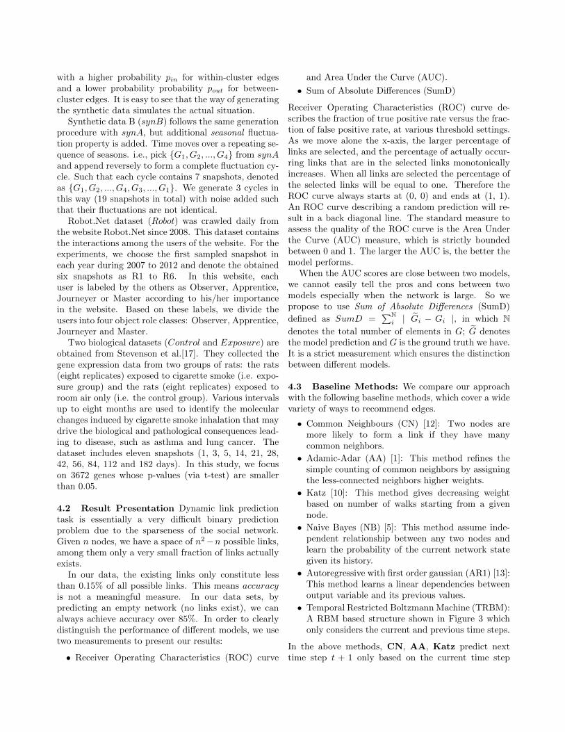
Figure 1: Examples of DegreeChange of synB (left),and Control (right). Y axis is the number of nodesin log scale (averaged between adjacent snapshots), Xaxis is the number of degree. A data point in this graphmeans the number of node changes (log scale) betweenadjacent snapshots in a particular degree slot.

results are shown in Section 4. We finally conclude thepaper in Section 5.

2 Problem Definition and Challenges

In this section, we present problem definitions andillustrate the challenges in real dynamic networks.

2.1 Problem Definition Given a series of snapshots{G1, G2, ..., Gt} of an evolving network Gt = (V, Et), weseek to predict the most likely link state in the next timestep, Gt+1. We assume that nodes V remain the sameacross all time steps but links Et change for each timet.

2.2 Challenges In this paper, we conduct experi-ments on five dynamic networks with different level ofdifficulties in which the first two are synthetic networksand the remaining are real world networks. While de-tails about the datasets and experiments can be foundin Section 4.1, we first illustrate the challenges in dy-namic networks that motivate our studies. The degreeproperties of these datasets are summarized in Table1 where the second and third column exhibit the aver-age and maximum degree of each network averaged overall the time steps, and the last column shows the totalnumber of links in each network.

For most of the dynamic networks, sparseness mea-sured by Node Degree varies from small to large. Dif-ferent level of sparseness brings a big challenge to the

V

W

H

a

b

Figure 2: A Restricted Boltzmann Machine

model robustness. This difficulty also occurs in ourdataset. i.e. Some node in Robot network shown inTable 1 has much sparser connections than others.

Nonlinear transformation is another challenge espe-cially for biological dynamic networks. To visualizecomplicated transitional informations, we define De-greeChange between two time steps Gi and Gi+k as theabsolute distance between the node degree distributionDist(Gi) and Dist(Gi+k), where D = Dist(G) com-putes the degree distribution of a single snapshot G sothat D(i) is the number of nodes of degree i. An ex-ample transition shown in Figure 1 describes the pair-wise difference (k = 1) between the first 6 snapshots(denoted as evoX) in synB and Control. As we can ob-serve, transitional patterns cannot be easily found espe-cially in the real data sets. It suggests that the proposedmodel should have the capabilities of modeling complexand nonlinear transition patterns.

3 Methodology

We have emphasized that models with distributed hid-den state are necessary for efficiently modeling complextimes series. However, this hidden states on directedmodels make the inference infeasible [2]. Therefore, ifwe use Restricted Boltzmann Machine (RBM) [8] basedmodels, the posterior over latent variables factorizescompletely which make the inference feasible. In thissection, we first review the RBM and propose a newmodel – Conditional Temporal Restricted BoltzmannMachine (ctRBM) which is able to absorb temporal vari-ations and neighbor opinions during the training phase,and make prediction conditioned on the current time-window and the expectation of local neighbors’ predic-tion. The model maintains the most important com-putational advantages which make the training efficientusing Contrastive Divergence algorithm [7].

The proposed method described in the followingsections will train a ctRBM denoted as Mp for each nodep, and finally get a collection of ctRBMs for all nodesdenoted as M. Therefore the final prediction, Gt+1, isobtained by collecting all the prediction results fromeach Mp. Although M makes a high space complexity,it can be easily deployed on large distributed platform.We will give further analysis in Section 4.

3.1 Restricted Boltzmann Machine RestrictedBoltzmann Machine (RBM) is a special case of MarkovRandom Field which has two layers of variables: V andH forming a fully connected bipartite graph with undi-rected edges as shown in Figure 2. RBM defines a dis-tribution over (V,H) ∈ {0, 1}NV × {0, 1}NH , where Vis the visible variables with dimension NV and H thehidden variables with dimension NH . This joint distri-bution is defined as:

(3.1)

P (V,H) = exp(V ′WH + a′V + b′H) / Z,

where Z =∑V,H

exp(V ′WH + a′V + b′H).

In this equation, W ∈ RNV ×NH is the weight betweenV and H, and the biases for V and H are a and baccordingly. Since there is no connection between nodesin each layer, the conditional distributions P (H | V )

and P (V | H) are fully factorial and given by

(3.2)P (Hj = 1 | V ) = σ(bj +W ′

:,jV ),

P (Vi = 1 | H) = σ(ai +Wi,:H),

where σ is the logistic function defined as σ(z) =(1 + exp(−z))−1, and i and j are the row and column

index. V is the reconstructed data, representing themodel’s estimation. The goal of learning is to minimizethe distance between V and V .

As with other models based on RBMs, the existenceof the partition function Z makes maximum likelihoodlearning intractable. Nonetheless, it is easy to computea good approximated gradient of an alternative objec-tive function called Contrastive Divergence[7]. This ap-proximation leads to a set of simple gradient updaterules. The updates for all W , a, and b parameters takethe form:

(3.3)

∆Wi,j ∝ 〈ViHj〉0 − 〈ViHj〉K ,

∆ai ∝ 〈Vi〉0 − 〈Vi〉K ,

∆bj ∝ 〈Hj〉0 − 〈Hj〉K ,

where 〈·〉0 defined as∑

EH|V [∂E(V,H)∂θ ] is an expecta-

tion with respect to the data distribution, and 〈·〉K de-

fined as∑

EV ,H [∂E(V,H)∂θ ] is an expectation with re-

spect to the joint distribution obtained from startingwith a training vector clamped to the observations andperforming K steps of alternating Gibbs sampling (i.e.CD-K). Typically K is set to 1, but recent results showthat gradually increasing K during learning can signifi-cantly improve performance at an additional computa-tional cost that is roughly linear in K [4].

3.2 Conditional and Temporal Property Nodes’transitional patterns and local neighbors’ influence canbe regarded as temporal and conditional property re-spectively. However, traditional RBM models can only

…

… W WA

aA

b

a

Vt-­‐N Vt-­‐1 Vt

Figure 3: A Restricted Boltzmann Machine with tem-poral information, where N is the window size.

model static frames of data. So for each node in thedynamic network, we propose to add two types of di-rected connections: temporal connections from thepast N configurations (time steps) of the visible units tothe current hidden configuration, and neighbor con-nections from the expectation of the local neighbors’predictions with respect to the the linkage history of thecurrent node.

This reformation makes a new powerful generativemodel, in which weights for temporal connections canmodel local nonlinear temporal structure very well,leaving the neighbor connection weights to model global,macro-level structure.

3.2.1 Temporal Connections As shown in figure3, we can model temporal dependencies by fixing thevisible variables in the previous N time slice(s). Thereexist similar RBM based models (e.g. [18], [19]) whichconsider history states. However, they are targetingon object features instead of linkage status which madetheir assumptions and updating procedures very differ-ent from the proposed model.

In the temporal connections, N is a tunable param-eter indicating how many time steps we need to lookback. In modeling high time resolution data, we can setN to be related to the frame rate such that the pro-posed model will be able to deal with evolutionary datastreams. To simplify the presentation, we will assumethe data at t−N , ..., t−1 is concatenated into a vectorV <t of dimension N · NV . Hence the weights for tem-poral connections are summarized by an N ·NV ×NHweight matrix called WA. By using this substitution, weavoid explicitly summing over past frames. Since theproposed model absorbs the temporary informations,the conditional probability will be changed to:

(3.4)P (Ht | V t, V <t; θ) = α · σ(b+W ′

AV<t) +

(1− α) · σ(b+W ′V t)

(3.5) P (V t | Ht) = σ(a+WHt),

where WA is the parameter for modeling the temporalvariations. α is a hyper parameter balancing the modelbehavior between conservative and progressive, we setit to be 0.5 in this paper.

…

… W WA

aA

b

ât

Vt-­‐N Vt-­‐1 Vt

ŋt at

Figure 4: The summarized neighbor influence ηt isintegrated into the energy function as adaptive bias.

3.2.2 Neighbor Connections It is commonlyknown that a person’s behavior will be affected byhis/her friends circle. In our problem setting, neigh-bors’ historical linkage behavior will indirectly affectthe future linkage status of node p. This phenomenoncan be simplified by the idea of Mean Field Theorythat the effect of all the other individuals on any givenindividual is approximated by a single averaged effect.Similarly, we can summarize local neighbors’ opinionsinto a unified one.

To formulate this idea, we define Neighbor Influenceas the expectation of its local neighbors’ predictions. Ifthe total number of nodes in V is n, then the NeighborInfluence can be defined as:(3.6)

ηtp =1

U tp

n∑q=1

l(xtp, xtq)× P (V t

q | Htq) · P (Ht

q | V tp , V

<tq ; θq),

where U tp =∑nq=1 l(x

tp, x

tq), and the indicator function

l is 1 if node q is linking to node p at time t, and 0otherwise. θq is the parameter of model Mq.

Neighbors make their predictions for node p base ontheir own experience (historical data). As we showed inEq.(3.6), averaged opinion ηtp of node p comes from itsneighbors’ opinions based on their own judgements (θqand V <tq ). Since models are already trained by previous

t− 1 snapshots, P (V tq | Htq) ·P (Ht

q | V tp , V <tq ; θq) can beeasily computed by Eq.(3.4)&(3.5) but substituting V t

in Eq.(3.4) by V tp .

3.3 Training and Inference on ctRBM Thanksto the complete factorable property over the latent vari-ables, training and inference in the ctRBM is no moredifficult than in the standard RBM. Specifically, thestates of the hidden units are determined by both theinput they receive from the individual observation V t

and V <t, and the input ηt they receive from neighbors,shown in Figure 4. Given V t and V <t, the hidden unitsat time t are conditionally independent, as in Eq.(3.4).The effect of the Neighbor Influence can be viewed asadaptive bias:

at = β · a+ (1− β) · ηt

which includes the static bias, a for the current obser-vation, and the contribution from the neighbors. β is ahyper parameter controlling individual to comply withthemselves or their friends, we set it to be 0.5 in thiswork. This equation modifies the bias of visible units:a in Eq.(3.5) is replaced with at to obtain:

(3.7) P (V t | Ht) = σ(at +WHt).

We can still use Contrastive Divergence for trainingthe ctRBM. The updates for the weights have the sameform as Eq.(3.3) but have a different effect because thestates of the hidden units are now influenced by V <t

and ηt. The gradients are now summed over all timesteps and updated by the following rules:

(3.8)

∆WA ∝∑t

(⟨V <tHt⟩

0−⟨V <tHt⟩

K),

∆aA ∝∑t

(⟨V <t⟩

0−⟨V <t⟩

K),

∆W ∝∑t

(⟨V tHt⟩

0−⟨V tHt⟩

K),

∆b ∝∑t

(⟨Ht⟩

0−⟨Ht⟩

K),

∆a ∝∑t

(β

1− β · (⟨V <t⟩

0−⟨V <t⟩

K) + ηt).

While inferencing on a ctRBM, we do not need to pro-ceed sequentially through the training data sequences.The future link status are only conditional on the pastN time steps and the neighbor influence. As long aswe fix the window size N , these small windows can bemixed and formed into mini-batches to speed up thelearning process.

3.4 Inferencing Linkage by ctRBM After train-ing, model parameters are fixed and predicting futurelink status follows the similar reason with inferencing.Specifically, we can shift the window one step towardsfuture to obtain a fixed observation which contains theprevious N−1 snapshots and the current snapshot. Wefix this known observation as history, calculate neighborinfluence based on a unified uncertainty (e.g. 0.5 for allunits) and perform a forward inference to get the net-work status at t + 1. The detailed procedure is shownin Algorithm 1.

As a property of generative models, a trained ctRBMcan fill in missing data if there are dropouts occur ina sequence, which may save us lots of time from datapreprocessing. The process is very similar to prediction.Formally, assume here is a missing snapshot Gd attime d. Given the known data ({G1 ∼ Gd−1} and{Gd+1 ∼ Gt}), we can first initialize their correspondingvisible units, then initialize the missing data to a unifieduncertainty (0.5 for all units) and alternate between

stochastically updating the hidden and visible units,with the known visible states held fixed.

Algorithm 1 Predicting Gt+1 by ctRBM

Input: A trained M for all nodes, in which Mp ∈M isparameterized by θp : {WAp,Wp, aAp, ap, bp}.A series of snapshots {Gt−N+1, ..., Gt}, where N isthe window size.

Output: Gt+1

1: p⇐ 1, Gt+1 ⇐ zeros(length(V), length(V))2: for p < length(V) + 1 do3: V <t+1

p ⇐ {Gpt−N+1, ..., Gpt }

4: V t+1p ⇐ ones(1, length(V))× 0.5

5: Get neighbor indices: Idx⇐ find(Gpt == 1)6: Get neighbor models list: Mnbr ⇐M(Idx)7: Calculate ηt+1

p by Eq.(3.6) given Mnbr

8: at+1p ⇐ ap + ηt+1

p

9: Calculate V t+1p by Eq.(3.4) & (3.7) substituting

V t and V <t by V t+1p and V <t+1

p

10: Gt+1p ⇐ V t+1

p

11: end for

3.5 Detecting Ill-behaved Nodes by ctRBMOne intrinsic ability of ctRBM is to detect ill-behavednodes. Because nodes with random behavior usuallyprovide less information. They randomly start andend relationship with other nodes which sabotage thenetwork stableness. Besides, nodes which add or deletea massive number of connections in a very short periodof time may indicate something significant, such as ashocking event happening in social network, or a seriousdeterioration of cancer. It would be meaningful to findthese nodes and events in real-time. However, linearmodels usually fails this task because there exist non-linear changing patterns of node degrees.

We can easily adapt the proposed model to enablethis functionality. For example, we can record the eu-clidean distance between the reconstruction V t (calcu-lated by Eq.(3.7)) and V t as t varies. Specifically, ifwe let the first sample to “burn-in” the proposed modeland start monitoring the distances for the rest, thenwill have a vector of size t − N where N is the win-dow size. We define this vector as ε. So, for each nodep, there is an εp recoding its “error pattern” along thetime dimension. Ideally, the numbers recorded in εpshould monotonically decrease to a very small residualbecause the proposed model fits the data better as timeincreases. However, the reconstruction may not be per-fect, i.e., there are abnormal behavior which disturb thereconstruction error.

As we aware, the majority of nodes are normal andpredictable. Therefore, the information for the majorityof items should also be reliable and consistent. We

thus derive the Consistency Score rp for each nodeas following:

(3.9) rp = ψ(εp,median(ε)),

where median(·) returns the error pattern of the ma-jority. ψ can be any distance function, we choose touse element-wised euclidean distance in this work. Asa result, rp will be a vector of the same length withεp. Under this measurement, the higher the score, thefurther the node is away from predictable.

We can simply rank the Consistency Score based on∑rp to find top problematic nodes. The distinction

between noise and sudden events is also easy amongthese problematic nodes, because the reconstructionerrors are consistently high across almost all the timesteps for noise, while only a small number of time stepsfor sudden events. In consequence, we can distinguishthem by setting a threshold, e.g., if more than 50% ofthe elements in εp are larger than the correspondingelements in median(ε), we can claim that node p isnoise.

3.6 Reducing the Prediction Time Algorithm 1indicates that for each node, prediction is made byconditioning on its past and all its neighbor opinions.The historical data can be absorbed by a fixed times ofmatrix multiplication which is in constant time, whilethe “consulting” dynamically changes over time becausethe neighbors of the node are changing. An interestingfinding is that in most of the real world datasets, nodedegrees are usually less than the square root of the totalnumber of links. e.g., the maximum node degree shownin Table 1. The computational complexity in this case isO(n

32 ). However, in the worst case scenario (e.g. when

a node connects to all other nodes), this complexityincreases to O(n2) which is not very efficient especiallywhen we want to do real-time prediction.

We address this problem based on a simple hypoth-esis, that the impact and influence from neighbors canbe clustered. There are two commonly known reasonssustaining this hypothesis. First, if two nodes sharesimilar neighbors, their Neighbor Influences will be sim-ilar. Second, group behavior is much more stable andpredictable than individual behavior. The hypothesisimplies that similar Neighbor Influences can be repre-sented by a center influence, and this centroid will notchange heavily over time. This idea can be implementedin a distributed fashion by the following procedure:

The tunable parameter k controls the updating in-terval, a rule of thumb is to set k = log(frame rate) forreal-time applications.

We name this procedure Neighbor Influence Cluster-ing (NIC) algorithm. In a word, this distributed ap-

Algorithm 2 Neighbor Influence Clustering

1: From the server, cluster ηt using any availableclustering algorithm after a few time steps from thebeginning (e.g. t = 5). Keep the resulting centroidsand node assignments as global.

2: Send the corresponding centroid to node p where pbelongs to, and replace ηtp ∼ ηt+kp by the centroid.

3: At time t + k + 1, each node sends request to itsneighbors to compute ηt+k+1, and find its nearestneighbor with the global centroids, then upload newassignments to the server.

4: Server updates node assignments and goes back tostep 2.

proximation algorithm reduce the computation cost bybucketing the neighbor influences into separate clustercentroids to avoid querying neighbor opinions for eachtime step. Theoretically speaking, the worst case run-ning time didn’t change when k equals to the frame rate.However, since k in practical is much smaller than theframe rate and irrelevant to the number of nodes, therunning time is very close to TRBM, which is O(n).

The initial position of these centroids will not verymuch affect the performance as long as they are sepa-rated. For the simplicity reason, we choose to use PCAand Kmeans to do clustering for the experiments. Apractical benefit of NIC is that it is deployable on largedistributed platform to handle millions of nodes.

4 Empirical Study

We first introduce our datasets and measurements, thenshow that our algorithm outperforms several baselinesin a variety of situations, such as noisy and seasonalityin link formation. These findings are confirmed on sev-eral evolving networks based on the evaluation metricsintroduced in Section 4.2.

4.1 Datasets We use the following five datasets inthe experiments.

Synthetic data A (synA) is generated based on theassumption that there are some common clusters withinthe network. For each snapshot, we generate 100 nodes,which are divided into five clusters of 20 nodes each, andthese nodes’ linkage behavior is sampled from predefineddistributions. If nodes belong to the same cluster, theirlinkage behavior is drawn from the same distribution.It is worth noticing that each cluster’s distribution maybe different with each other. Moreover, a controllablepart of nodes are randomly chosen to be the onessampling from outlier distributions. All the nodes arethen shuffled with noises are added. From the 2nd tothe 19th snapshots, edges are added/deleted randomly

with a higher probability pin for within-cluster edgesand a lower probability probability pout for between-cluster edges. It is easy to see that the way of generatingthe synthetic data simulates the actual situation.

Synthetic data B (synB) follows the same generationprocedure with synA, but additional seasonal fluctua-tion property is added. Time moves over a repeating se-quence of seasons. i.e., pick {G1, G2, ..., G4} from synAand append reversely to form a complete fluctuation cy-cle. Such that each cycle contains 7 snapshots, denotedas {G1, G2, ..., G4, G3, ..., G1}. We generate 3 cycles inthis way (19 snapshots in total) with noise added suchthat their fluctuations are not identical.

Robot.Net dataset (Robot) was crawled daily fromthe website Robot.Net since 2008. This dataset containsthe interactions among the users of the website. For theexperiments, we choose the first sampled snapshot ineach year during 2007 to 2012 and denote the obtainedsix snapshots as R1 to R6. In this website, eachuser is labeled by the others as Observer, Apprentice,Journeyer or Master according to his/her importancein the website. Based on these labels, we divide theusers into four object role classes: Observer, Apprentice,Journeyer and Master.

Two biological datasets (Control and Exposure) areobtained from Stevenson et al.[17]. They collected thegene expression data from two groups of rats: the rats(eight replicates) exposed to cigarette smoke (i.e. expo-sure group) and the rats (eight replicates) exposed toroom air only (i.e. the control group). Various intervalsup to eight months are used to identify the molecularchanges induced by cigarette smoke inhalation that maydrive the biological and pathological consequences lead-ing to disease, such as asthma and lung cancer. Thedataset includes eleven snapshots (1, 3, 5, 14, 21, 28,42, 56, 84, 112 and 182 days). In this study, we focuson 3672 genes whose p-values (via t-test) are smallerthan 0.05.

4.2 Result Presentation Dynamic link predictiontask is essentially a very difficult binary predictionproblem due to the sparseness of the social network.Given n nodes, we have a space of n2−n possible links,among them only a very small fraction of links actuallyexists.

In our data, the existing links only constitute lessthan 0.15% of all possible links. This means accuracyis not a meaningful measure. In our data sets, bypredicting an empty network (no links exist), we canalways achieve accuracy over 85%. In order to clearlydistinguish the performance of different models, we usetwo measurements to present our results:

• Receiver Operating Characteristics (ROC) curve

and Area Under the Curve (AUC).

• Sum of Absolute Differences (SumD)

Receiver Operating Characteristics (ROC) curve de-scribes the fraction of true positive rate versus the frac-tion of false positive rate, at various threshold settings.As we move alone the x-axis, the larger percentage oflinks are selected, and the percentage of actually occur-ring links that are in the selected links monotonicallyincreases. When all links are selected the percentage ofthe selected links will be equal to one. Therefore theROC curve always starts at (0, 0) and ends at (1, 1).An ROC curve describing a random prediction will re-sult in a back diagonal line. The standard measure toassess the quality of the ROC curve is the Area Underthe Curve (AUC) measure, which is strictly boundedbetween 0 and 1. The larger the AUC is, the better themodel performs.

When the AUC scores are close between two models,we cannot easily tell the pros and cons between twomodels especially when the network is large. So wepropose to use Sum of Absolute Differences (SumD)

defined as SumD =∑Ni | Gi − Gi |, in which N

denotes the total number of elements in G; G denotesthe model prediction and G is the ground truth we have.It is a strict measurement which ensures the distinctionbetween different models.

4.3 Baseline Methods: We compare our approachwith the following baseline methods, which cover a widevariety of ways to recommend edges.

• Common Neighbours (CN) [12]: Two nodes aremore likely to form a link if they have manycommon neighbors.

• Adamic-Adar (AA) [1]: This method refines thesimple counting of common neighbors by assigningthe less-connected neighbors higher weights.

• Katz [10]: This method gives decreasing weightbased on number of walks starting from a givennode.

• Naive Bayes (NB) [5]: This method assume inde-pendent relationship between any two nodes andlearn the probability of the current network stategiven its history.

• Autoregressive with first order gaussian (AR1) [13]:This method learns a linear dependencies betweenoutput variable and its previous values.

• Temporal Restricted Boltzmann Machine (TRBM):A RBM based structure shown in Figure 3 whichonly considers the current and previous time steps.

In the above methods, CN, AA, Katz predict nexttime step t + 1 only based on the current time step

0.15 0.2 0.25 0.3 0.35 0.4 0.45 0.5 0.55 0.6 0.65

0.5

0.6

0.7

0.8

0.9

1 AUC scores over increasing noise

Percentage of noise

AU

C s

core

ctRBMTRBMKatz−awCN−awAA−awKatz−auCN−auAA−auAAKatzCN

TRBM

AA, Kartz, CN

ctRBM

Figure 5: The performances on SynA with increasingpercentage of noise added.

5 10 50 100 500 10000

0.2

0.4

0.6

0.8

1

Number of hidden units

AccuracyAUC

Figure 6: The perfor-mance on models with dif-ferent expression capacity.

1 8 16 32 48 640

0.5

1

1.5

2

2.5

3

Number of Cores

Run

ning

Tim

e (s

)

ExposureControlRobotSynA

Figure 7: The speed upachieved by using morecores.

t. We denote their variations as CN-au, AA-au andKatz-au, where the notion -au means “all previoussnapshots till time t are equally (unweighted) consideredand used”. We denote another variations of them asCN-aw, AA-aw and Katz-aw which use decayingweight for all previous snapshots when they are awayfrom the current. NB and AR1 are under the samesituation as the models with “au”.

4.4 Experiments We first test the noise toleranceof ctRBM against several baselines on distorted SynA.Specifically, we randomly flip the linkage of all nodesby a designated percentage. As shown in Figure 5,ctRBM consistently outperforms all the other baselinesby a large margin. We observe that CN, AA and Katzbehaves as bad as random predictor. This is becauseof their limitations of predicting t + 1 only based on t,which is biased. TRBM also outperforms other heuristicbaselines. However, the reason of performance gapexists between ctRBM and TRBM is because TRBMdid not consider the global information.

Performance Test. Table 2 compares all theperformances over the five datasets described in Section

4.1, in which ctRBM-k is the proposed model withNeighbor Influence clustered. We achieve the bestamong all baselines even if the network is very sparse(Robot), or with non-linear patterns (SynB). Aninterest finding is that AR1 performs very well on Robot.This is because the user interactions on Robot.Netevolve very slowly (changes are small and gradual), andthe gaussian noise assumption fits the data. However, ithas the worst performance on biological networks whichhave much more complicated variations. The missingitems for Control and Exposure are simply because ofthe cubic time complexity.

Noisy Node Detection Test. To test our anomalydetection method, we manually pick some nodes inSynA and randomly flip their linkage behavior across alltime. Since we know their indices, we can use accuracyto measure how many ill-behaved nodes are correctlycaptured. We find in Figure 6 that the proposed modelcan perfectly detect these nodes when the number ofhidden units fit the data.

Parameter Sensitivity Test. The number ofhidden units is closely related to the representationalpower of ctRBM. Figure 6 shows the performance ofctRBM under different parameter settings. When thenumber of hidden units is small, the model is lackof capacity to capture data complexity which resultsin lower performance on both detection accuracy andprediction. In contrast, the number is too large that wedon’t have sufficient samples to train the network whichresults in a even lower performance and stability. Infact, the parameter tuning is all about balancing modelcapacity with insufficient number of samples. In thiscase, we choose 100 to be the “sweet point”.

Speedup Test. The proposed method (ctRBMwith NIC) is implemented on a high-performance clustercontaining a large number of computation units whereeach unit has CPU of 8 cores. We acquire 8 unitsand test our algorithm on 4 datasets. As shown inFigure 7, the running times keep decreasing when weinvolve more cores. However, the curve of SynA goesup after 8 because the inter-core communication timestarts to dominate. Theoretically, we can always finda balance point which can maximize the performancewhile minimize the computation cost.

5 Conclusions

In this paper, we proposed a generative model – ctRBMfor dynamic link prediction. The proposed model suc-cessfully captures the complex variations and nonlineartransitions such as seasonal fluctuations, and it can alsoperform direct inference to predict future linkage with-out nearest neighbor searches. The proposed Neigh-bor Influence Clustering (NIC) algorithm further re-

Table 2: Comparison with Baselines Using SumD and AUC

SynA SynB Robot Control Exposure

AA 2424 (0.7125) 2296 (0.7206) 6158 (0.5016) 368101 (0.6342) 524511 (0.5711)AA-au 2702 (0.7127) 2368 (0.7125) 6157 (0.5016) - -AA-aw 2808 (0.7103) 2488 (0.7179) 6158 (0.5016) - -CN 3314 (0.5059) 3178 (0.5243) 6158 (0.5000) 643326 (0.5303) 902037 (0.5392)CN-au 2078 (0.7230) 2828 (0.5801) 6157 (0.5000) - -

baseline CN-aw 1954 (0.7024) 2848 (0.5766) 6158 (0.5000) - -Katz 2306 (0.7232) 2292 (0.7195) 6140 (0.5011) 369450 (0.6138) 528556 (0.5389)Katz-au 2168 (0.7291) 1874 (0.7531) 6142 (0.5010) - -Katz-aw 2194 (0.7318) 1930 (0.7474) 6140 (0.5011) - -NB 3109 (0.5704) 3314 (0.5831) 6209 (0.5000) 365405 (0.6545) 519117 (0.5409)AR1 2993 (0.6056) 1775 (0.8680) 19 (0.991) 787301 (0.5054) 940974 (0.5021)TRBM 384 (0.9322) 684 (0.9109) 0 (1.000) 76648 (0.7902) 85944 (0.7302)

proposed ctRBM 210 (0.9641) 411 (0.9427) 0 (1.000) 61302 (0.8103) 69912 (0.7882)approach ctRBM-k 259 (0.9574) 464 (0.9441) 0 (1.000) 68843 (0.8028) 78843 (0.7727)

duces the practical running time of prediction to O(n).The measurement defined in NIC can also be applied ontransitional patterns so that the proposed ctRBM modelcan be used to detect malfunction nodes easily. Ex-perimental results on synthetic and real world datasetsshow that ctRBM outperforms existing link predictionalgorithms on dynamic networks. The proposed ctRBMmodel provides a powerful analytic tool for understand-ing the transitional and evolutionary behavior of dy-namic networks.

References

[1] L. A. Adamic and E. Adar. Friends and neighbors onthe web. Social networks, 2003.

[2] C. C. Aggarwal, Y. Xie, and S. Y. Philip. On dynamiclink inference in heterogeneous networks. In SDM,2012.

[3] L. E. Baum and T. Petrie. Statistical inference forprobabilistic functions of finite state markov chains.The annals of mathematical statistics, 1966.

[4] M. A. Carreira-Perpinan and G. E. Hinton. Oncontrastive divergence learning. In AISTATS, 2005.

[5] R. Caruana and A. Niculescu-Mizil. An empiricalcomparison of supervised learning algorithms. InICML, 2006.

[6] Z. Ghahramani and G. E. Hinton. Variational learningfor switching state-space models. Neural computation,2000.

[7] G. E. Hinton. Training products of experts by minimiz-ing contrastive divergence. Neural computation, 2002.

[8] G. E. Hinton and R. R. Salakhutdinov. Reducing thedimensionality of data with neural networks. Science,2006.

[9] P. Indyk and R. Motwani. Approximate nearest neigh-bors: towards removing the curse of dimensionality. InSTOC, 1998.

[10] L. Katz. A new status index derived from sociometricanalysis. Psychometrika, 1953.

[11] N. D. Lawrence. Gaussian process latent variablemodels for visualisation of high dimensional data.NIPS, 2004.

[12] D. Liben-Nowell and J. Kleinberg. The link-predictionproblem for social networks. JASIST, 2007.

[13] T. C. Mills. Time series techniques for economists.Cambridge University Press, 1991.

[14] V. Pavlovic, J. M. Rehg, and J. MacCormick. Learningswitching linear models of human motion. In NIPS,2000.

[15] P. Sarkar, D. Chakrabarti, and M. Jordan. Nonpara-metric link prediction in dynamic networks. arXivpreprint arXiv:1206.6394, 2012.

[16] U. Sharan and J. Neville. Temporal-relational clas-sifiers for prediction in evolving domains. In ICDM,2008.

[17] C. S. Stevenson, C. Docx, R. Webster, C. Battram,D. Hynx, J. Giddings, P. R. Cooper, P. Chakravarty,I. Rahman, J. A. Marwick, et al. Comprehensive geneexpression profiling of rat lung reveals distinct acuteand chronic responses to cigarette smoke inhalation.AJP-LUNG, 2007.

[18] I. Sutskever and G. E. Hinton. Learning multileveldistributed representations for high-dimensional se-quences. In AISTATS, 2007.

[19] G. W. Taylor and G. E. Hinton. Factored conditionalrestricted boltzmann machines for modeling motionstyle. In ICML, 2009.

[20] T. Tylenda, R. Angelova, and S. Bedathur. Towardstime-aware link prediction in evolving social networks.In SNAKDD, 2009.

[21] D. Q. Vu, D. Hunter, P. Smyth, and A. U. Asun-cion. Continuous-time regression models for longitu-dinal networks. In NIPS, 2011.