A CUTTING PLANE ALGORITHM FOR SOLVING

BILINEAR PROGRAMS

Hiroshi Konno

December 1974 WP-74-75

Working Papers are not intended fordistribution outside of IIASA, andare solely for discussion and infor-mation purposes. The views expressedare those of the author, and do notnecessarily reflect those of IIASA.

1. Introduction

Nonconvex programs which have either nonconvex minimand and/or

nonconvex feasible region have been considered by most mathematical

programmers as a hopelessly difficult area of research. There are,

however, two exceptions where considerable effort to obtain a global

optimum is under way. One is integer linear programming and the other

is nonconvex quadratic programming. This paper addresses itself to a

special class of nonconvex quadratic program referred to as a 'bilinear

program' in the lieterature. We will propose here a cutting plane

algorithm to solve this class of problems. The algorithm 1S along the

lines of [17] and [19] but the major difference is in its exploitation of

special structure. Though the algorithm is not guaranteed at this stage

to converge to a global optimum, the preliminary results are quite

encouraging.

In Section 2, we analyze the structure of the problem and develop

an algorithm to obtain an £-locally maximum pair of basic feasible

solutions. In Section 3, we will generate a cutting plane to eliminate

current pair of £-locally maximum basic feasible solutions. We use, for

these purposes, simplex algorithm intensively. Section 4 gives an

illustrative example and the results of numerical experimentations.

2. Definitions and a Locally Maximum Pair

of Basic Feasible Solutions

The bilinear program is a class of quadratic programs with the

following structure:

- 2 -

(2.1)

n. m. m. x n. nl

x n2where c

i' xi £ R ~, bi £ R ~, Ai £ R ~ ~,i = 1, 2 and C £ R

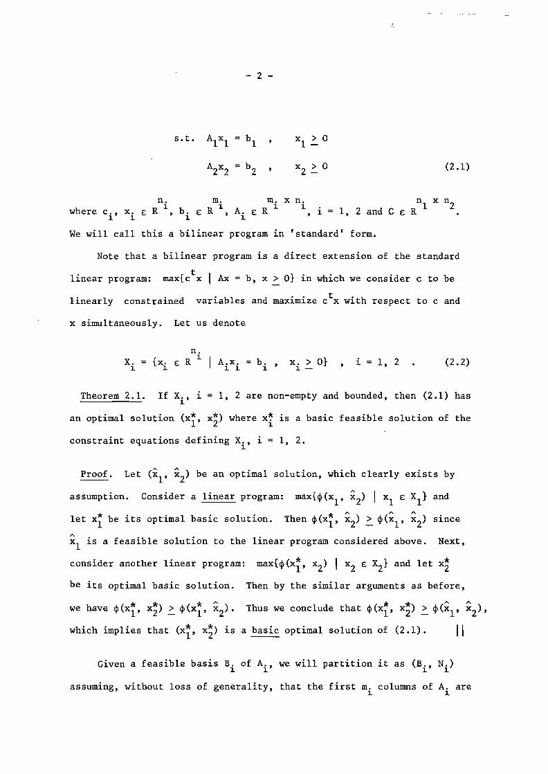
We will call this a bilinear program in 'standard' form.

Note that a bilinear program is a direct extension of the standard

linear program: max{ctx I Ax = b, x ~ o} in which we consider c to be

linearly constrained variables and maximize ctx with respect to c and

x simultaneously. Let us denote

A.x. = b. , x. > o}~ ~ ~ ~ - i = 1, 2 (2.2)

Theorem 2.1. If X., i = 1, 2 are non-empty and bounded, then (2.1) has~

an optimal solution (xi, x~) where xi is a basic feasible solution of the

constraint equations defining X., i = 1, 2.~

Proof. Let (Xl' x2) be an optimal solution, which clearly exists by

assumption. Consider a linear program:

let xi be its optimal basic solution.

max{~(xl' x2) I xl £ Xl}

* A "A

Then ~(xl' x2) ~ ~(xl' x2)

and

since

~l is a feasible solution to the linear program considered above. Next,

consider another linear program: max{~(xi, x2) I x2 £ X2} and let x~

be its optimal basic solution. Then by the similar arguments as before,

we have ~(xi,

which implies

* *" * * ""x2) ~ ~(xl' x2)· Thus we conclude that ~(xl' x2) ~ ~(xl' x2),

that (xi, x~) is a basic optimal solution of (2.1). II

Given a feasible basis B. of A., we will partition it as (B., N.)~ ~ ~ ~

assuming, without loss of generality, that the first m. columns of A. are~ ~

- 3 -

basic. Position xi correspondingly: xi = (xiB , xiN). Let us introduce

here a 'canonical' representation of (2.1) relative to a pair of feasible

1 . l' B-1 h . .Premu t1.p Y1.ng . to t e constra1.nt equat1.on1.

B,x' B + N,x' N = b. and suppressing the basic variables x1.'B' we get the1. 1. 1. 1. 1.

following system which is totally equivalent to (2.1):

s. t.

(2.3)

where

For future reference, we will introduce the notations,

i.ii = n i - mi , di = c iN E R 1.

i.Yi = xiN E R 1.

-1 m. x i. -1 m.R 1. 1. 1.F. = B . N. E f. = B . b. E R1. 1. 1. 1. 1. 1.

il x i Z

<Po0 0

D = C E R = <P(xl , x2)

and rewrite (2.3) as follows:

i = 1, 2

s.t.

Y2 ~ 0 (Z.4)

We will call (2.4) a canonical representation of (2.1) relative to (Bl , B2)

and use standard form (2.1) and canonical form (2.4) interchangeably

whichever is the more convenient for our presentation. To express the

- 4 -

dependence of vectors in (2.4) on the pair of feasible bases (Bl , B2),

we will occasionally use the notation dl (Bl

, B2), etc.

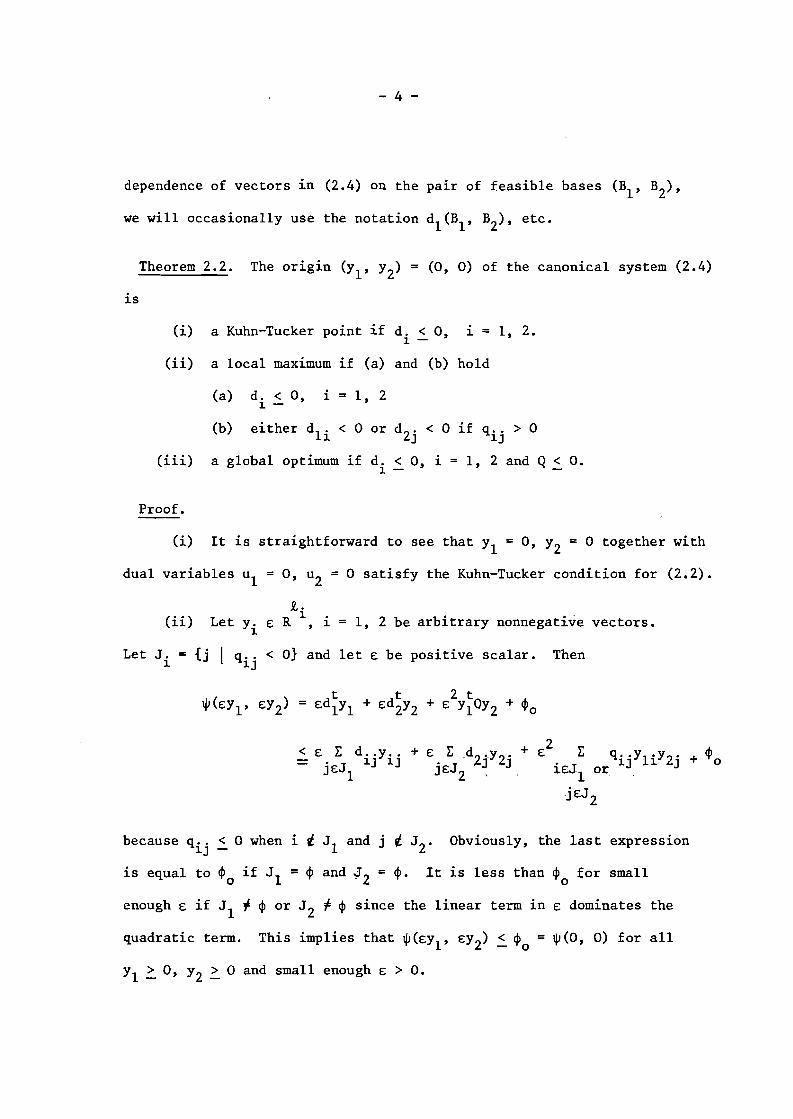
Theorem 2.2. The origin (Yl' Y2) = (0, 0) of the canonical system (2.4)

is

(i) a Kuhn-Tucker point if d. < 0,1. -

1. = 1, 2.

(ii) a local maximum if (a) and (b) hold

(a) d. < 0,1.- i = 1, 2

(iii)

Proof.

(b) either dli < 0 or d 2j < 0 if qij > 0

a global optimum if d. < 0, i = 1, 2 and Q < O.1.-

(i) It is straightforward to see that Yl = 0, Y2 = 0 together with

dual variables ul = 0, u2 = 0 satisfy the Kuhn-Tucker condition for (2.2).

R,.(ii) Let Yi £ R 1., 1. = 1, 2 be arbitrary nonnegative vectors.

Let J. = {j I q .. < O} and let £ be positive scalar. Then1. 1.J

< £ I: d ..y .. + £ I: ,d2 .Y2. + £2 I: q1..J. Yl1.·Y2J. + <Po= J·cJl 1.J 1.J J·cJ2 J J . J~ ~ 1.£1 or .

j£J2

because q .. < 0 when i i J l and j i J 2 • Obviously, the last expression1.J -

is equal to <Po if J r = <P and J 2 = <p. It is less than <Po for small

enough £ if J l + <P or J 2 + <P since the linear term in £ dominates the

quadratic term. This implies that ~(£Yl' £Y2) ~ <Po = ~(O, 0) for all

Yl ~ 0, Y2 ~ 0 and small enough £ > O.

- 5 -

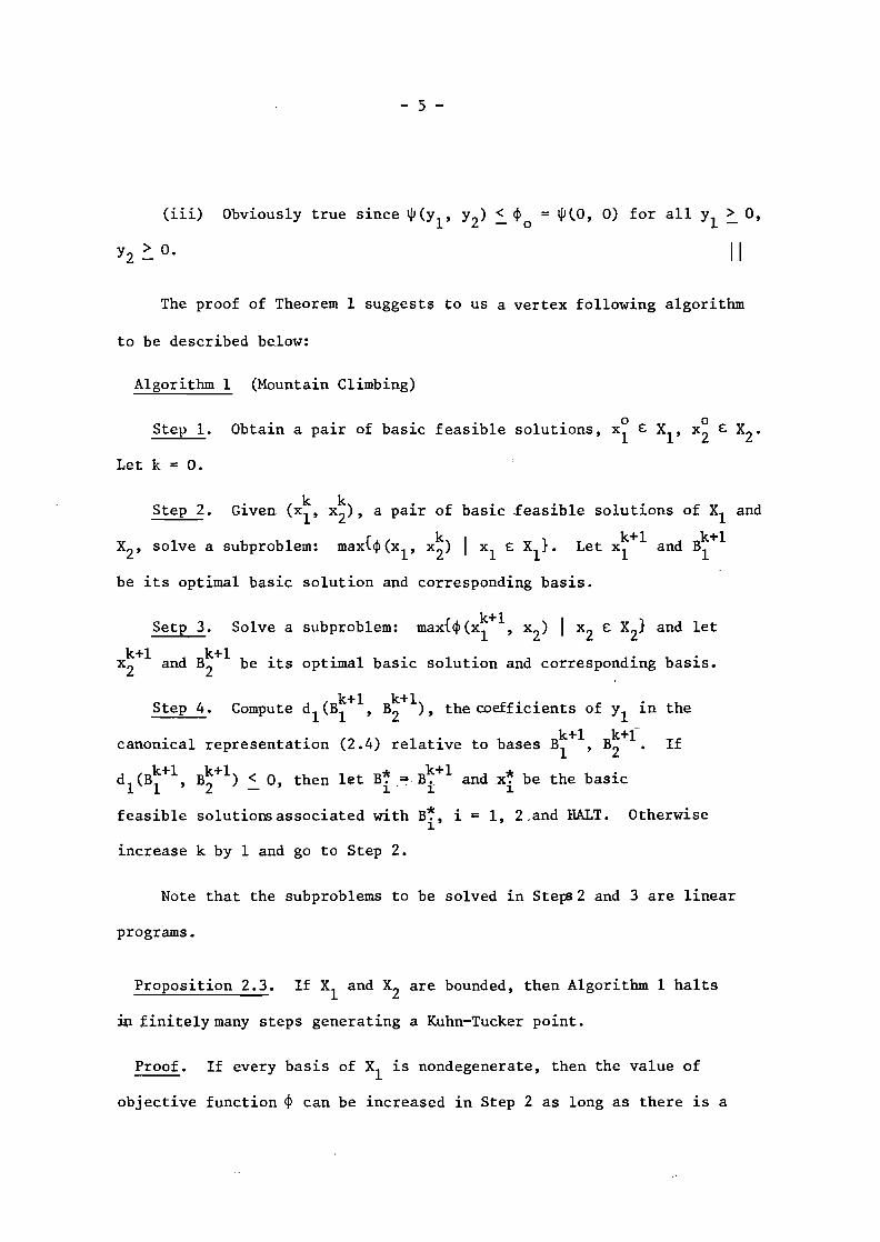
(iii) Obviously true since ~(Y1' YZ) ~ ~o = ~lO, 0) for all Yl ~ 0,

Yz ~ o. II

Algorithm 1

The proof of Theorem 1 suggests to us a vertex following algorithm

to be described below:

(Mountain Climbing)

Step 1.

Let k = O.

o 0Obtain a pair of basic feasible solutions, xl E Xl' Xz E XZ•

Step Z. k kGiven (x1,xZ), a pair of

XZ' solve a subproblem: max{~(x1' x~)

basic feasible solutions of Xl

I k+1 Bk+1xl E Xl}· Let xl and 1

and

be its optimal basic solution and corresponding basis.

{ k+1 ISetp 3. Solve a subproblem: max ~(x1 ,xZ) Xz E XZ} and let

x~+l and B~+l be its optimal basic solution and corresponding basis.

S 4 d (Bk+1 k+l) eff· . f htep . Compute 1 1 ,BZ ,the co 1C1ents 0 Yl 1n t e

Bk+1 Bk+fcanonical representation (Z.4) relative to bases 1 ' Z • If

d (Bk+1 k+1) < 0 h 1 t B* Bk+1 d * b the basic1 1 ,BZ _' t en e i .",!, i an xi e

feasible solutions associated with B~, i = 1, Z.and HALT. Otherwise1

1ncrease k by 1 and go to Step Z.

Note that the subproblems to be solved in StepsZ and 3 are linear

programs.

Proposition Z.3. If Xl and Xz are bounded, then Algorithm 1 halts

in finitely many steps generating a Kuhn-Tucker point.

Proof. If every basis of Xl is nondegenerate, then the value of

objective function ~ can be increased in Step Z as long as there is a

- 6 -

positive component in dl • Since the number of basis of Xl is finite and

no pair of bases can be visited twice because the objective function is

strictly increasing in each passage of Step 2, the algorithm will eventually

.. .. (k+l Bk+l) . ..term1nate w1th the cond1t1on dl BI '2 ~ 0 be1ng sat1sf1ed. When Xl is

degenerate, then there could be a chance of infinite cycling among certain

pairs of basic solutions. We will show however,,:that this cannot happen

in the above process if we employ an appropriate tie breaking device in

linear programming. Suppose

optimal basis Bk+lI

k+R.-l)max{ <p (xl' x2 .

k+R.where x k+l

x for the first time 1n the cycle. Since the value of

objective function <p is nondecreasing and

( k+l k+R.) (k+l k+l)- <p xl ,x2 ~ <p xl ,x2

we have that

k+l k+l) k+2 k+l) k+R. k+R.)<P(xi ' x2 = <p (xl ' x2 = . . . . = <P(x1 ' x2

It is . ( k+l k+lthe definition optimality ofobv1ous that d2 BI ' B2 ) ~ 0 by of

Bk+l Suppose that the jth k+l k+l) is positive. Then2 • component of dl(BI ' B2

standard form, the

k+la t xl and hence

k+lfor xl = xl and

- 7 -

we could have introduced y .. into the basis. However, since the objective1J

function should not increase,y .. comes into the basis at zero level.1J

Hence the vector Yl remains zero. We can eliminate the positive element

of dl

, one by one, (using tie breaking device for the degenerate LP if

necessary) with no actual change in the value of Yl. Eventually, we have

"'k+ld2 ~ 0 with Yl = 0 and the corresponding basis B

l• Referring to the

corresponding xl value remains unchanged i.e., stays

-k+l k+l k+l . .d2 (B

l,B

2) ~ 0, because B

21S the opt1mal basis

"':k+l k+lthat xl = xl • By Theorem 2 (i), the solution

obtained is a Kuhn-Tucker point.

Let us assume 1n the following that a Kuhn-Tucker point has been

II

obtained and that a canonical representation (2.4) relative to associated

pa1r of bases has been given.

By Theorem 2 (iii), that pa1r of basic feasible solutions is optimal

if Q < o. We will assume that this is not the case and let

K = {(i, j) I q .. > O}1J

Let us define for (i, j) £ K, a function $ .. : R2

+ R1J +

Proposition 2.4. If 111 •• (~ ,11) > 0 for some ~ > 0,11 _> 0, then'l'1J"O 0 "0 - 0

$. '(~' 11) > $(~ • 11 ) for all ~ > ~ • 11 > 111J 0 0 0 0

Proof.

(~ - ~ )(dl · + q··11 )o 1 1J 0

+ (11- 11 )(d2 · + q .. ~ ) + q .. (~ - ~ )(11 - 11 )o J 1J 0 1J 0 0

- 8 -

+ q .. (~ - ~ )(n - n )~J 0 0

> ° II

This proposition states that if the objective function increases in the

directions of Ylj and Y2j

, then we can ~ncrease more if we go further into

this direction.

Definition 2.1. Given a basic feasible solution x. £ X., let N.(x.)~ ~ ~ ~

be the set of adjacent basic feasible solution which can be reached from

x. in one pivot step.~

Definition 2.2. A pa~r of basic feasible solutions (x~, x~), x~ £ Xi'

i = 1, 2 is called an £-locally maximum pair of basic feasible solution if

(i)

(ii)

d. < 0, i = 1, 2~ -

In particular this pa~r is called a locally maximum pa~r of basic feasible

solutions if £ = 0.

Given a Kuhn-Tucker point (x~, x;), we will compute $(xl

, x2) for all

x. £ N.(x~), ~ = 1, 2 for which a potential increase of objective function~ ~ ~

$ is possible. Given a canonical representation, it is sufficient for

this purpose to calculate ~ .. (t., n.) for (i, j) £ K where t. and n.~J ~ J ~ J

represent the maximum level of nonbasic variables x1j

and x2j

when they

are introduced into 'the bases without violating feasibility.

- 9 -

Algorithm 2. (Augmented Mountain Climbing)

Step 1. Apply Algorithm 1 and let x~ EX., 1 = 1, 2, be the resulting1 1

pair of basic feasible solutions.

Step 2. If (x~, x;) is an E-locally maximum pair of basic feasible

solutions, then HALT. Otherwise, move to the adjacent pair of basic feasible

and go to Step 1.

3. Cutting Planes

We will assume 1n this section that an E-locally maximum pair of basic

feasible solutions has been obtained and that a canonical representation

relative to this pair of basic feasible solution (x~, x;j has been given.

Since we will refer here exclusively to a canonical representation, we

will reproduce it for future conven1ence:

(3.1)

where d. < 0, f. > 0, 1 = 1, 2. Let1 - 1-

LY. = {yo E R 1

1 1F. y. < f., y. > O}11- 1 1- i = 1, 2 (3.2)

Y ~R,)R,.

{Yo E R 1 I Yu ~ 0, y .. = 0, J :f R,}1 1 1J

R, = 1, .... , L. i 1, 21

i.e. y~R,) is the ray emanating from Yi = ° in the direction YiR,.

(3.3)

- 10 -

Lemma 3.1. Let

(3.4)

If ~l(u) > 0 for some u £ Y~~), then ~l(v) > ~l(u) for all v £ Y~~) such

that v > u.

Proof. Let u = (0, ... , 0, u~, 0, ••• , 0). First note that u~ > 0

tsince if u~ = 0, then ~l(u) = max{d2y I Y2 £ Y2} = o.

Let v = (0, ... , 0, v~, 0, •.. , 0) where v~ ~ u~. Then for all

Y2 £ Y2, we have

The inequality follows from d2 ~ O. Thus

12~

j=l

12~

j=l

q1j Y2j

(d2j + qtjU t )Y2jI

II

This lemma shows that the function ~l is a strictly increasing function

of y on y(1) beyond the point where ~l first becomes positive.1 1

- 11 -

<P + E:-max

Figure 3.1 Shape of the Function ~l

Let ~ be the value of the objective function associated with themax

best feasible solution obtained so far by one method or another and let

1us define a~, ~ = 1, ... , ~l as follows:

1at = max a for which

{ IU ( ) I y(~)max "I l Yl Yl E: 1 ' o ~ Ya ~ a} ~ ~max + e: (3.5)

Lemma 3.2. a~ > 0, ~ = 1, .•. , ~l.

Proof. Let Yl = (0, ••. , 0, Yl~' 0, ..• , 0). Since dl ~ 0, d2 ~ 0, we

- 12 -

have

Letting a = max{~qijY2j I Y2 £ Y2} ~ 0, we know from the above inequality

that

> (~ - ~ + £}/a > 0- 'I'max '1'0

= + co

Theorem 3.3. Let

a > 0

a = 0 II

1Y1 ./6. < 1,

J J-(3.6)

Then

Proof. Let

6~ if 6~ is finite~1 J J6. =

J6~6 if =co

0 J

Y2 £ Y2} < ~ + E. - 'I'max

(3.7)

where 6 > 0 is constant.

Then

The right hand side term inside the limit is a bilinear program with bounded

feasible region and hence by Theorem 2.1, there exists an optimal solution

- 13 -

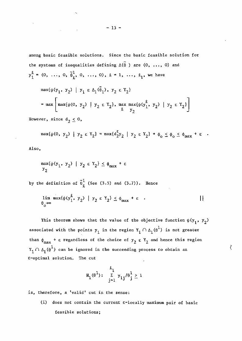
among basic feasible solutions. Since the basic feasible solution for

-the systems of inequalities defining ~(8 ) are (0, •.• , 0) and

~ -1Yl = (0, .•. , 0, e~, 0, ••. , 0), ~ = 1, ••• , ~l' we have

However, since d2 ~ 0,

tmax{d2Y2 I Y2 £ Y2} + ~ < ¢ < ¢ + £'flo - 0 - max

Also,

max{~(Yl' Y2) I Y2 £ Y2} ~ ¢max + £Y2

by the definition of e~ (See (3.5) and (3.7». Hence

This theorem shows that the value of the objective function ~(Yl' Y2)

associated with the points Yl in the region Yl n ~1(8l) is not greater

than ¢max + £ regardless of the choice of Y2 £ Y2 and hence this region

1Yl n ~l(e ) can be ignored in the succeeding process to obtain an

£-optimal solution. The cut

1HI (8 ):

~l

l:j=l

1Yl . /8. > 1

J J-

1S, therefore, a 'valid' cut in the sense:

(i) does not contain the current £-locally maximum pair of basic

feasible solutions;

- 14 -

(ii) contains all the candidates Yl £ Yl

for which

since 81 is dependent on the feasible region YZ

' we will occasionally use

the notation 8 l (yZ).

Since the problem is symmetric with respect to Yl

and YZ

' we can,

if we like, interchange the role of Yl

and YZ

to obtain another valid

cutting plane relative to YZ:

Cutting Plane Algorithm

ZYZ./8. = 1

J J

Step O. Set t = O. Let X?1.

X.,i=l,Z.1.

Step 1. Apply Algorithm Z (Augmented Mountain Climbing Algorithm)

with a pair of feasible. t t

reg1.ons Xl' XZ·

1 t t+l t~ 1 t t+l$,Step Z. Compute 8 (YZ). Let Yl = Yl til (8 (YZ))· If Y

l=

stop. Otherwise proceed to the next step.

Step Z'. (Optional).Z t+l

Compute 8 (Yl

).

If y~+l = ¢, stop. Otherwise proceed to the next step.

Step 3. Add 1 to t. Go to Step 1.

It is now easy to prove the following theorem.

Theorem 3.4. If the cutting plane algorithm defined above stops in

Step Z or Z', with either yt +l or ytZ

+l becoming empty, then ¢ and1 max

- 15 -

associated pair of basic feasible solutions are an E-optimal solution

of the bilinear program.

Proof. Each cutting plane added does not eliminate any point for which

the objective function is greater than ¢max + E.., t+1

Hence 1f e1ther Yl

t+2or Y2 becomes empty, we can conclude that max{~(Yl' Y2) I Yl E Yl , Y2 E Y2}

< ¢ + E.- max

According to this algorithm, the number of constraints increases by

II

1 whenever we pass step 2 or 2' and the size of subproblem becomes bigger

and the constraints are also more prone to degeneracy. From this viewpoint,

we want to add fewer number of cutting planes, particularly when the

original constraints have a good structure (e.g. transporation~. Insuch

case, we might as well omit step 2' taking Y2

as the constraints having

special structure.

Another requirement for the cut is that it should be as deep as

possible, in the following sense:

Definition 3.1. Let e = (e. ) > 0, 1: = (1:. ) > 0. Then the cutJ J

'[.Yl./e. > 1 is deeper than '[.y1 ·IT. . > 1 if e ~ 1:, with at least oneJ J- J J

component with strict inequality.

Looking back into the definition (3.5) of e1, it is clear that

e1 (U) ~ el(V) when U C V C R.t2 and that the cut associated with e1

(U) is

1 . 1deeper than e (V). Thus, given a pair of valid cuts HI (e (Y

2» and

H2 (e2

(yl », we can use YZ Y2'\f:.2 (e2

(yl » C Y2 and Yi = Yl",f:.

l(e l (y

2»

1 2CYI to generate Hl(e (YZ» and H2 (e (Yi» which are deeper than the cuts

associated with Y2 and Yl • This iterative improvement scheme is very

powerful especially when the problem is symmetric with respect to Yl

- 16 -

and YZ. This aspect will be discussed in full detail e1sewhe;~ [llJ.

1The following theorem gives us a method to compute a using the

dual simplex method.

Theorem 3.5.

1 "{ t ( )}an = m1n -d z +. -. + E Z .Jt., max 0 0

= 1

(3.8)

Z" > 0, j = 1, ••• , R.Z' Z > 0J - 0-

Proof. Let

g(a)

an 1S then given as the maximum of a for which g(a) < • -. + E.Jt., - max 0

It is not difficult to observe that

where qR.­

which

t= (qu' ••• , qR.R. ) •

2Therefore, ai is the maximum of a for

< tf, - tf, + E- 'I'max '1'0

- 17 -

The feasible region defining glee) 1S, by assumption, bounded and

non-empty and.by duality theo~em

Hence e~ 1S the maximum of e for which the system

1S feasible, i.e.,

e~ = max e

u > 0

This problem is always feasible and again uS1ng duality theorem,

ten = min -dZz + (¢ - ¢ + £)z

N max 0 0

Z _> 0, Z > 00-

with the usual understanding that e~ = + 00 if the constraint set above

is empty. II

Note that dZ < 0 and ¢ - ¢ + £ > 0 and hence (z, z ) = (0, 0)- max 0 - 0

is a dual feasible solution. Also the linear program defining ei 1S

only one row different for different ~, so that they are expected to be

solved without exceeding amount of computation.

- 18 -

Though it usually takes only several pivotal steps to solve (3.8),

it may be necessary, however, to pivot more for large scale problems.

However, since the value objective function of (3.8) approaches to its

minimal value monotonically from below, we can stop pivoting if we like

when the value of objective function becomes greater than some specified

value. Important thing to note is that if we pivot more, we tend to get

a deeper cut, in general.

4. Numerical Examples

The figure below shows a simple 2 dimensional example:

C -)(21)+ (xU' x12

)1 x

22-1

s. t.

~1~8 2 1(X2~

,x12 ~ 1 2 x22 ~

1 1

There are two locally maX1mum pairs of basic feasible solutions 1.e.,

(PI' Ql) and (P4 , Q4) for which the value of objective function 1S 10 and

13, respectively. We applied the algorithm omitting step 2'. Two cuts

generated at PI and P4 are shown on the graph. In two steps, x~ = ~ and

the global optimum (P4 , Q4) has been identified.

A NUMERICAL EXAMPLE- 19 -

3

2

//

1

y\CUT GENERATED AT p"

1 1 >14.44 J:11 + 1.45 x12=

1

3

2

1

/2/

OPTIMAL SOLUTION( P4 , Q 4 ) : 'P *=13

LOCALLY MAXIMUM PAIROF b. f. s.

(P 1 ,Q 1) : rp =10

4 x 11 + x12 =12/

4

- 20 -

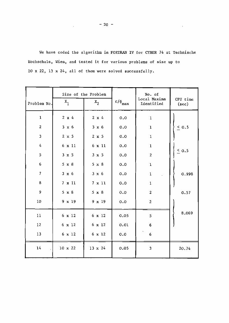
We have coded the algorithm in FORTRAN IV for CYBER 74 at Technische

Hochschule, Wien, and tested it for various problems of size up to

10 x 22, 13 x 24, all of them were solved successfully.

Size of the Problem No. of

Xl X2 £!¢maxLocal Maxima CPU time

Problem No. Identified (sec)

1 2 x 4 2 x 4 0.0 1

2 3 x 6 3 x 6 0.0 1 < 0.5-3 2 x 5 2 x 5 0.0 1

4 6 xU 6 x U 0.0 1< 0.5

5 3 x 5 3 x 5 0.0 2 -

6 5 x 8 5 x 8 0.0 1

7 3 x 6 3 x 6 0.0 1 0.998

8 7 xU 7 xU 0.0 1

9 5 x 8 5 x 8 0.0 2 0.57

10 9 x 19 9 x 19 0.0 2

U 6 x 12 6 x 12 0.05 58.069

12 6 x 12 6 x 12 0.01 6-,

13 6 x 12 6 x 12 0.0 6

14 , 10 x 22 13 x 24 0.05 3 20.74

- 21 -

Problem 2 is taken from [20]. and problem 9 from [2J. 11 tV 13

are the same problems having six global maxima with eElual value. These

are in fact global optima. The data for this problem is given below:

tb2

= (21, 21, 21, 21, 21, 21)

2 -1 0 0 0 0 1 2 3 4 5 6 I 1 0 0 0 0 0I

-1 2 -1 0 0 0 2 3 4 5 6 1 10 1 0 0 0 0

0 -1 2 -1 0 0 3 4 5 6 1 210 0 1 0 0 0c = Al = A2

= I0 0 -1 2 -1 0 4 5 6 1 2 3 1 0 0 0 1 0 0

0 0 0 -1 2 -1 5 6 1 2 3 410 0 0 0 1 0I

0 0 0 0 -1 2 6 1 2 3 4 51 6 0 0 0 0 11" l'

A 160

This is the problem associated with convex maximization Frob1em

max{!xtCx I A x < b, x < O}o -

Data for problem 14 was generated randomly.

- 22 -

REF E R E.N C E S

[lJ Altman, M. "Bilinear Programming," Bulletin d'Academie Polonaisedes Sciences, Serie des Sciences Math. Astr. et Phys., 19No.9 (1968), 741-746.

[2J Balas, E. and Burdet, C-A. "Maximizing a Convex Quadratic FunctionSubject to Linear Constraints," Management Science ResearchReport No. 299, GSIA, Carnegie-Mellon University, July 1973.

Cabot, A.V. and Francis, R.L.Minimization Problems by18 No.1 (1970), 82-86.

"Solving Certain Nonconvex QuadraticRanking Extreme Points," J. ORSA

[5J

[8J

[9]

[10]

ell]

Charnes, A. and Cooper, W.W. "Nonlinear Power of Adjacent ExtremePoint Methods in Linear Programming," Econometrica, 25 (1957),132-153.

Candler, W. and TownsleY,R.J. "The Maximization of a QuadraticFunction of Variables Subject to Linear Inequalities,"Management Science, 10 No.3 (1964), 515-523.

Cottle, R.W. and Mylander, W.C. "Ritter's Cutting Plane Methodfor Nonconvex Quadratic Programming," in Integer and NonlinearProgramming (J. Abadie, ed.) North Holland, Amsterdam, 1970.

Dantzig, G.B. "Solving Two-Move Games with Perfect Information,"RNAD Report P-1459, Santa Monica, California, 1958.

Dantzig, G.B. "Reduction of a 0-1 Integer Program to a BilinearSeparable Program and to a Standard Complementary Problem,"Unpublished Note, July 27, 1971.

Falk, J. "A Linear Max-Min Problem," Serial T-25l, The GeorgeWashington University, June 1971.

Gallo, G. and tllkllcll, A. "Bilinear, Programming: An ExactAlgorithm," Paper presented at the 8th InternationalSymposium on Mathematical Programming, August 1973.

Konno, H. "Ma;x:imization of Convex Quadratic.F.unction underLinear Const.rai,n.ts'," \olill.be.subrnittep. asa~ IIASA working

. paper, November 19]4.. . .

Konno, H. "Bilinear Programming Part II: Applications ofBilinear Programming;'Technical Report No. 71-10, Departmentof Operations Research, Stanford University, August 1971.

- 23 -

[13J Mangasarian, O.L. "Equilibrium Points of Bimatrix Games," J. Soc.Indust. App1. Math, ~ No.4 (1964), 778-780.

[14J Mangasarian, O.L. and Stone, H. "Two-Person Nonzero-Sum Games andQuadratic Programming," J. Math. Anal. and Appl., 2. (1964),348-355.

[15] Mills, H. "Equilibrium Points in Finite Games," J. Soc. Indust.App1. Math., ~ No.2 (1960), 397-402.

[16J My1ander, W.C. "Nonconvex Quadratic Programming by a Modificationof Lemke's Method," RAC-TP-414, Research Analysis Corporation,McLean, Virginia, 1971.

[17J Ritter, K. "A Method for Solving Maximum Problems with a NonconcaveQuadratic Objective Function," Z. Wahrschein1ichkeitstheorie,verw. Geb., ± (1966), 340-351.

[18J Raghavachari, M. "On Connections between Zero-one Integer Programmingand Concave Programming under Linear Constraints," J. ORSA, 17No.4 (1969), 680-684.

[19J

[20J

Tui, H. "Concave Programming under Linear Constraints," SovietMath., (1964), 1437-1440.

Zwart, P. "Nonlinear Programming: Counterexamples to Two GlobalOptimization Algorithms," J. ORSA. 21 No.• 6 (1973), 1260-12

[21J Zwart, P. "Computational Aspects of the Use of Cutting Planes inGlobal Optimization," Proc. 1971 Annual Conference of the ACM(1971), 457-465.