A CRITICAL REVIEW OF SINGLE FUELAND INTERFUEL SUBSTITUTION RESIDENTIAL

ENERGY DEMAND MODELS

RAYMOND S. HARTMAN

March 1978

MIT ENERGY LABORATORY REPORT - MIT-EL-78-003

PREPARED FOR THE UNITED STATES

DEPARTMENT OF ENERGY

Under Contract No. EX-76-A-01-2295Task Order 37

ABSTRACT

The overall purpose of this paper is to formulate a model of residential

energy demand that adequately analyzes all aspects of residential consumer en-

ergy demand behavior and properly treats the penetration of new technologies,

particularly solar photovoltaics, in an explicit fashion. An adequate treat-

ment of energy demand must take account of the fact that both fuel demand and

the demand for fuel-burning equipment are jointly derived from the demand for

fuel related services. This requires modelling both demand for fuels and for

their related equipment. In order to model the equipment demand and the demand

for new technologies, the technological characteristics of the alternative

equipment must be explicitly analyzed. The formulated model attempts such

explicit analyses.

In order to formulate such a model this paper first introduces and reviews

19 existing residential energy demand models to ascertain how well they have

dealt with these issues.

i

PREFACE

The research discussed in this paper reflects work undertaken by the

author as part of a larger analysis of the potential markets for solar photo-

voltaics. That larger analysis has been and is being conducted by the MIT En-

ergy Laboratory for the Department of Energy, formerly the Energy Research and

Development Administration.

The author would like to express gratitude for the extremely helpful sug-

gestions of David Wood and Richard Tabors.

The author is an Assistant Professor of Economics at Boston University,

and a member of the Research Staff of the MIT Energy Laboratory. The author

completed this research while at the MIT Energy Laboratory.

ii

CONTENTS

A) INTRODUCTION AND SUMMARY

B) MODEL CRITERIA

C) REVIEW OF MODELS OF DEMAND FOR INDIVIDUAL FUELS

D) REVIEW OF INTERFUEL SUBSTITUTION DEMAND MODELS

E) SUMMARY AND STATEMENT OF FURTHER RESEARCH

BIBLIOGRAPHY

iii

-1-

A) INTRODUCTION AND SUMMARY

The activity of critically reviewing a group of positive or normative models

of the social or physical sciences can be a thankless task for several reasons.

In the first place, the process of model review usually takes the approach of

constructive criticism; as a result, while aimedrat being constructive, the cri-

ticism is still criticism and can affront those modellers whose models are reviewed.

In the second place, the review function perforce limits the body of models dis-

cussed to those felt to be most relevant to the particular purposes at hand; as

a result,the review can also affront those who feel certain crucial or seminal

efforts have been excluded.

In spite of these potential difficulties, I attempt to identify and critically

review a group of energy demand models in this paper for two major objectives.

1) The first objective is to indicate how various analysts have understood

and modelled the demand for energy by residential users. Since the demand for

energy is a derived demand given the demand for the services that a given energy

source provides (such as heating, cooking, and clothes drying for residential

consumers), the analysis of energy demand must deal with the fact that fuels and

fuel burning appliances are combined in varying ways to produce a particular resi-

dential (and commercial and industrial) service. As a result, analysis of the

demand for energy must include analysis of the interactive demands for both fuel

burning capital and the fuel used by that capital stock. This review of energy

demand models will assess how and how well the reviewed models deal with both of

these demands.

2) This review is performed for the Department of Energy in order to

develop improved energy demand models for the analysis of the penetration of new

energy technologies, in particular solar photovoltaic installations for residential

-2-

use. As a result a second objective of the review is to identify the analytic

strengths and weaknesses of the assembled models with respect to their usefulness

in explicitly analyzing the demand for new energy technologies.

The literature provides a wide array of models available for this review.

Over the past ten to fifteen years, quantitative models of the system of sources

and uses of various energy forms have come to dominate an increasing share of the

engineering, management research, and economic literature. The literature now

abounds with old and new models of supply and demand, with characterizations and

assessments of new technologies. The research area has been legitimized by a

number of review articles such as Hoffman and Wood ( 50 ) and Charles River Asso-

ciates ( 25 ).

These models have been developed in order to understand, quantify and finally

to predict technological, sociological, and/or economic behavior and relationships

underlying an energy system. The desires to understand, quantify, and predict have,

at times, been stimulated by academic interest. At other times, the modelling

efforts have been intended either to do or to evaluate strategic planning acti-

vities and policy analysis. For example, state, local and federal regulatory

bodies (FPC, ERDA, FEA, state utility commissions, EPA, CEQ, etc.) affect utility

rate structures, environmental compliance costs, research and development into a

diffusion of new technologies, pipeline and utility siting, and appliance efficiency

standards and taxes, to name just a few. At times the policy planning of these

agencies is based upon ad hoc decisions; in other cases, the quantitative models

are utilized to help refine and understand the impacts of proposed policy measures

(see 58, 34, 63, 44). Likewise, quantitative models have been utilized to do or to

evaluate strategic planning for energy industries or other private sector parti-

cipants (21).

-3-

A number of techniques have been utilized in the construction of these energy

models including optimizing techniques (linear, non-linear and integer programming

- 27, 18), activity analysis and input-output analysis (59, 48, 72), statistical

and econometric techniques and engineering/process methods (10, 58, 49). Many

models or analyses utilize only one of these techniques; however, others combine

several of the techniques.

As indicated above, it is the purpose of this paper to review those models

that focus upon the residential/commercial sectors. All the models deal with

energy demand; the review will indicate how well the models deal with new techno-

logies and the fundamental fact that the demand for energy related services in-

volves demand for fuels and fuel burning equipment.

The demand models to be reviewed can:be divided into two groups:

* models dealing with demand for a single fuel

* models dealing with overall energy demand and interfuel substitution

The models that are reviewed in these categories are listed in Table 1.

While this table contains 19 modelling efforts (enough for any review), the

list is clearly not exhaustive. For example, the translog utility analyses of

consumer demand characterized by the efforts of Christensen, Jorgenson and Lau

and Berndt, Darrough and Diewert1 are not included. The reasons for their exclu-

sion become clear when the proposed model respecifications are discussed in Section E.

The single fuel demand models analyze the demand for one fuel, usually elec-

tricity. In general, the single fuel demand models are more refined in their

1 See E.R. Berndt, M.N. Darrough and W.E. Diewert (1977) "Flexible FunctionalForms and Expenditure Distributions: An Application to Canadian Consumer DemandFunctions," International Economic Review, (October, 1977) and Christensen, L.K.,Jorgenson, D.W., and Lau, L.J., "Transcendental Logarithmic Utility Function,"The American Economic Review, Vol. 65, #3 (June 1975) pp. 367-383.

-4-

TABLE 1: MODELS REVIEWED IN SECTIONS C AND D

SINGLE FUEL MODELS INTERFUEL SUBSTITUTION MODELS

Acton, Mitchell and Mowill(19376), (AMM)

Anderson (1972), (1973)

Balestra (1967)

Cargill and Meyer (1971), (CM)

Fisher and Kaysen (1962), (FK)

Griffin (1974)

Halvorsen (1973)

Houthakker (1951)

Houthakker, Verleger, Sheehan(1!974), (HVS)

Mount, Chapman and Tyrrell(1973), (MCT)

Mount and Chapman (1974), (MC)

Taylor, Blattenberger, Verleger/DRI (1977), (TBV)

Willis (1977)

Wilson (1971)

Baughman/Joskow (B/J)

Federal Energy AdministrationProject Independence EvaluationSystem (FEA/PIES)

Oak Ridge/Hirst, et al.(OR/H)

Anderson

Erickson, Spann and Ciliano(ESC)

-5-

analytic structure and data base. For example, Mount, Chapman and Tyrrell (MCT)

incorporate variable elasticities that change with the level of the explanatory

variables. Acton, Mitchell and Mowill (AMM) and Fisher and Kaysen (FK) utilize

a multi-equation specification of demand focusing upon the demand for fuel-burning

capital and a separate specification for the demand for a fuel given that fuel-

burning capital. The Taylor,Blattenberger, Verleger/DRI (TBV)analysis of resi-

dential electricity demand develops marginal and fixed electricity charges.

In spite of their refinement these single fuel models deal inadequately with

the competition from other fuels and from new technologies-through price cross-

elasticities only. The models dealing with interfuel substitution explicitly are

theoretically superior because they are based upon the premise that the demand for

any fuel cannot be adequately assessed without quantifying the price and non-price

competition to that fuel posed by all alternative fuels and their respective fuel-

burning appliances. However, in spite of the theoretical superiority of these

interfuel substitution models, the empirical implementation of them has been

deficient to date. The analytic refinement and data base development of the single

fuel models are missing in the interfuel substitution models. For the most part,

interfuel comparisons are based only upon operating costs (2,3,4,5,6,9,10,12,58,

13,35), while the capital costs and technological characteristics of alternative

fuel burning devices have been ignored (except in 60 and 45).

These characteristics of the single fuel and interfuel substitution demand

models will be explored in greater detail in the actual review sections C and D

below. Based upon that review, one must conclude that in spite of the theoretical

superiority of the interfuel substitution models, and in spite of the fact that the

single fuel demand analyses provide great analytic refinement, extended efforts

are still required. The entire generation of energy demand models in the liter-

ature have reached a stage of forced obsolescence. New work done on consumer

-6-

choice modeling (generalized logit [Hartman ( 43) and covariance probit

[Hausman and Wise ( 47 )], production/cost duality [Econometrica International

( 33 )], and the explicit differences between short-run and long-run energy

demand [DRI ( 29 )] provides extremely cogent arguments for completely respeci-

fying the analyses of energy demand in order to adequately model the penetration

of new technologies such as solar photovoltaics within a well specified demand

model.

Such a respecification is currently being performed by the MIT Energy Lab

for the Department of Energy. The goals of the respecification are based directly

on model characteristics explored in the critical review in sections C and D.

That respecification is outlined heuristically in Section E. To summarize, that

respecification will include the following objectives:

* Explicit dichotomization of the behavioral characteristics and policy

variables for short-run and long-run demand.

It was stated above that the demand for energy related services articulates

itself in demand for fuels and fuel-burning equipment. The different behavioral

characteristics of demands for fuels and for equipment must be properly incor-

porated. In the short-run, the characteristics and size of the energy-burning

capital stock are fixed. Behavioral specifications and policy variables must take

into account that demand responses can only take the form of conservation and

altered capital utilization. In the long-run, when the size and characteristics

of the capital stock are variable, the characteristics of new technologies and

interfuel substitution (through changes in the capital mix) become relevant.

Likewise in the long-run, appliance efficiency taxes and standards, and appliance

capital costs become relevant policy variables in addition to the standard opera-

ting costs of the fuels.

-7-

* Utilization of appropriate models and data for consumer choice.

Conditional logit has been utilized extensively for the analysis of inter-

fuel substitution in a partial adjustment framework. However, conditional logit

as used in the literature suffers from a number of difficulties including: the

imposition of constant cross-elasticities [see Baughman and Joskow ( 9, 11, 12,

13 ), Hausman ( 46 ), Domencich and McFadden (32 ), Hartman ( 43), and Hart-

man and Hollyer (45 )]; implied misspecification [Hartman and Hollyer ( 45 )

and Hartman (43 )]; excluded variables; and the restrictive underlying model of

individual choice [Hartman (43 ) and Hartman and Hollyer ( 45 )]. Such modeling

of consumer choice could be improved by generalized logit formulations [Hartman

( 43 )] or covariance probit formulations [Hausman and Wise (47 )]. Further-

more the choice methodologies could be applied to changes in the appliance stock

rather than the actual stock [see Hartman and Hollyer ( 45 )].

* Appropriate treatment of new technologies.

While generalized logit and covariance probit avoid some of the difficulties

inherent in conditional logit, the treatment of new technologies is not trivial

for either new alternative and careful formulation is required.

The discussion in this review proceeds as follows. Because the purpose of

the discussion is to critically review the energy demand models identified in

Table 1, Section B introduces a number of model criteria to assist in that review.

Utilizing those criteria Section C reviews the demand analyses that focus upon

individual fuels and Section D reviews the interfuel substitution models. Finally,

Section E summarizes the model evaluation and proposes the nature and scope of

model reformulation desirable for better treatment of new technologies (solar

photovoltaics in particular).

-8-

B) MODEL CRITERIA

The purpose of the model review is to evaluate the models in Table 1, their

treatment of demand, and their ability to assess new technologies. Such an eval-

uation requires some formulation, explicit or implicit, of criteria with which the

models can be judged. It is the purpose of this section to introduce a set of

such criteria.

Eight criteria for the evaluation of modelling energy demand are introduced

and discussed here. The criteria are generally stated; specific articulation for

the actual models is found in Sections C and D. These criteria can be utilized

at two levels:

* Evaluation of a given model of energy demand against an idealized stand-

ard of comparison.

* Evaluation of a given model against the purported desires and scope of the

modellers.

The two levels of evaluation serve different purposes. The evaluation of a model

against the purported modelling aims of the model-developers indicates just how

well the model-developers were able to specify, quantify, develop, and utilize the

analytic system they desired. Such an evaluation is very important to model users

familiar with the analytic and policy aims of a given model. However, a more on-

erous model evaluation - against an idealized standard of comparison - is also

very useful. While a given model may be well-suited for the particular analyses

intended by the model-developers, crucial policy questions and crucial market

and geographical disaggregations may have been ignored in the initial aims of

modelers.

The eight criteria for energy demand models to be used in the review are as

follows:

i) Proper identification of major market participants and the level of dis-

-9-

aggregation required.

While this review focuses upon residential energy demand, some of the inter-

fuel substitution models analyze other user sectors as well; hence it is useful

to indicate other user sector disaggregations. Four sectors of final use include

commercial, residential, industrial and transportation use. One area of intermed-

iate use is the electric utility sector. Residential use can be disaggregated by

type of use (home-heating, water heating, cooling, etc.). Commercial and indus-

rial use can be disaggregated by process and comfort use while industrial users

can be disaggregated by SIC or technological characteristics.

In most cases, the greater the disaggregation by user sector and fuel use,

the better. However, extreme disaggregation may not be useful for all analytic

purposes; as a result the thrust of this criteria will depend upon the analytic

aims of the modelers.

ii) Proper identification and incorporation into variables in the model of

policy issues and technological considerations for the major market participants.

One of the two principal concerns of this model review is to examine the ab-

ility of models to assess the competitiveness of new energy technologies and anal-

yze alternative energy policy proposals for the penetration of those technologies.

As a result, a crucial criterion is whether the important policy and technological

issues have been properly incorporated into the variables and the structure of the

models.

The policy issues in general are most easily dichotomized into long-run and

short-run issues. In the short-run, a model of energy demand should deal with

conservation techniques and policy variables aimed at affecting the utilization

of a given stock of fuel-burning equipment (e.g., thermostat control, highway

speed limits, appliance use standards). In the long-run, where new technology

penetration is crucial, a demand model should deal with such policy and technical

-10-

issues as the explicit characteristics of technologies, efficiency standards

(taxes) and the effect of them upon changes in the stock of fuel-burning equip-

ment.

iii) Proper degree of geographical disaggregation.

As with criterion i), greater geographical disaggregation is generally bet-

ter. However, the actual level of disaggregation is more usefully judged against

the analytic aims of the model builder.

iv) Utilization of the appropriate behavioral models and underlying behav-

ioral assumptions.

The second principal concern of this review is the appropriate treatment of

the dual components of energy demand; to wit demand for fuels and for fuel-burning

equipment. Given the identification of the major market participants and the pol-

icy and technical issues to be addressed, a wide array of analytic specifications

are available for demand analysis; they include partial adjustment models, choice

models, consumer utility models, etc. While each type of model provides a power-

ful tool for analyzing a particular behavioral phenomenon, each model also imposes

certain assumptions upon the behavior being analyzed. Such assumptions require

critical scrutiny before a model is estimated and utilized for policy. Futher-

more, the available analytic specifications can be complicated; as a result, the

details of the technical application of the behavioral models also require close

scrutiny.

v) Proper integration of the demand analysis into an overall energy and/or

macroeconomic model.

This criteria is applicable only to those single fuel or interfuel substitu-

tion demand models that are utilized within larger models of energy systems. For

purposes of this review, this criterion will be relevant only to several of the

interfuel subsitution demand analyses. In those cases, a well-specified energy

-11-

demand module must be properly integrated into a well-specified overall model of

energy in order to simultaneously assess the static interaction of demand and

supply and dynamic changes in demand and supply over time.

vi) Utilization of proper data and statistical/econometric techniques.

A comprehensive and well-specified model may prove useless if improper his-

torical data and/or estimation techniques are used. It is not usually possible

(given research budget constraints) to subject a given model to rigorous statis-

tical testing including forecasting; backcasting; estimation for sub-sample of

data to test parameter estimate robustness; and examination of alternative vari-

ables and specifications. However, such analysis can be very useful in assessing

the adequacy of the data and the estimation techniques.

Furthermore, in policy simulation, the inputted exogenous variables must ad-

equately represent the policy scenarios being assessed.

vii) Provision of good documentation for the use of the energy demand model-

ling.

viii) Provision for relatively easy accessibility and extensibility of the

modelling effort.

It is not possible for a given model or group of modelers to incorporate or

foresee all possible policy simulations or analytic uses. As a result, it is a

very desirable characteristic that it is easy to enter the theoretical and com-

puter-coded structure of a model in order to alter or extend particular elements

of that model for specific analyses desired by the potential user.

-12-

C) MODELS OF DEMAND FOR INDIVIDUAL FUELS

OVERVIEW

In Section A, the Introduction and Summary, it is stated that the demand

models would be reviewed to assess their treatment of the dual components of de-

mand - demand for fuels and demand for fuel-burning capital stock. Furthermore,

the models will be assessed regarding their treatment of new technologies. Both

assessments focus upon the behavioral structure of the models.

In Section B, criterion iv) indicated that there exist many behavioral models

for dealing with energy demand. Several of these behavioral models are discussed

here. Before that discussion, it is useful to summarize the consumer demand be-

havior that the models attempt to approximate. That behavior can be thought of as

a three step process that spans both the long-run and the short-run:

* The consumer decides whether to buy a fuel-burning consumer durable, cap-

able of providing a particular consumer service (e.g. cooking, heating,

lighting, air conditioning, etc.)

* The consumer decides on the characteristics of the equipment he desires,

including efficiency, technical characteristics and fuel type. The con-

sumer also decides on whether the equipment is a new or traditional tech-

nology.

* Once the equipment is acquired, the consumer determines the frequency and

intensity of use.

The first two decisions, which are sometimes simultaneous, are essentially

long-run decisions that effect changes in the size and characteristics of the

fuel-burning capital stock. The third decision is short-run, taking the capital

stock as given.

This Section will indicate how each of the single fuel models approximates

these three consumer behaviors.

-13-

The models to be reviewed in this section were introduced in Table 1 of Section

A and are repeated in Table 2 along with a brief summary of their characteristics.

Table 2 delineates a number of important characteristics of the reviewed

models. The level of analysis is usually residential electricity or electrical

applicance demand, although some results for residential/commercial electricity

demand and gas demand are also reported. The type of data utilized by the mod-

els is usually pooled time-series cross-sectional data for states; however, a num-

ber of studies utilize more refined disaggregated data at the county meter read-

book level. The dependent variable of the single equation models is usually elec-

tricity consumption on a total, per capita, per household or per customer basis.

In some cases, demand for the appliance stock and demand for gas and oil are also

modeled. In one case [Taylor, Blattenberger, Verleger/DRI (29)] study, the de-

pendent variable is the utilization rate of the appliance stock. The explanatory

variables in the models usually include own-price (Po), substitute prices (P),

income (Y), population (N), weather/climate variables (W), appliance stock data

(A), demographic variables (including housing characteristics, degree of urban-

ization and characteristics of the consuming residences) (D), and a time trend (t).

Examples of static and dynamic models are included. For dynamic formulations,

stock adjustment specifications utilizing a lagged endogenous variable are common

in the models reviewed. In some cases, appliance prices are also used. The func-

tional form and estimation techniques are identified in Table 2. The price speci-

fication is indicated, since in the face of the declining block rate electricity

prices, a number of alternative price specifications can be used with different

theoretical and empirical implications.

Since the principal reason for this review is to assess the validity of the

behavioral assumptions about energy demand inherent in these models particularly

-14-

TABLE 2: OVERVIEW OF DEMAND STUDIES

1) ATONI, ITOIELLAND .OVILL (1976)

2) ANIERSON (972)

3) ANDESON (1973)

4) BALESTIA (1967)

UOALYSIALYSES

IX7EL OF AInLTSSI/TYE OF DATA

DlEVARIAL pa P.

ANATOr DVARIAt I· · W A D. t

IUnCTIONAL FORM/ESTIMATION TECNIQU

RESIDENTIAL LECTRICIT CONSUIIPTION By . X · I Z I I LINAR; TOTAL ENERGT EQALLZGDEMAD II0S3nLD N E PRODUCT Of THE APFLIACE

STOCK AND ITS UTILIZATION IAT. .MINHL DATA FOR ME 130 3 CROSS-SECTIONAL AND TIE-READ OOK AREAS IN LOS SERIES ANALYSIS SEPARATELY.AUImf.ES COUNTY, JULY 1972JUl1E 1974 _ _ _..

RESIDENTIAL ELECTRICIT!DEUA;D

30 STATES, 1969 ANNUAL CONSUMPTION 1 I I 1 LO -LIEAR, oPER FLEXIBLE (NEW)

CALIFORNIA, ANNUALL CUSTOMER IN I lr I 1947-1969 /CUSTOMER YEAR _ _ _

RESIDENTIAL APPLIANCE, oSHARES OF X I I I I lto-LImnAR, OLS AND aS.ELECTRICITY, GAS APPLIANCE STOCK IT STATIC AND DYNAXICDEMAND ENERGYCI TYPE FOR IHULATIONS

SO STATES, 1960-1970 VAIOUIIS USESoDRAIND FOR I X X I

OUSEHOLD* ..oIMaDFOCAS I I I I I

RESIDIIAL/COIMEECIAL GAS IN STO 1012; · X LAGGD LINR. LOG-LINEAR, FIRSTGAS DEMAND INCRaENTAL DEMAND DEPENDENT DIFFERENCES, 2SLS, FrAX

49 STATES AND AID TOTAL DEMAND VARILZ LIEIHOOD. PARTIALuASlNCGTON, D.C. ADJUSTMET rFOMULATOs19S-1962

5) CAIGILL AD ELECTRICITY DEMAND FOR STE tOAD AT 1 I 1 O N O 0 24 OU.LY EQUATIONS; OLSIETEI (1971) ALL SECTORS t - , I - 1,.... 4. PRODUCTION

2 SMSA'S, UNTHLT DESEASONALIZED WORKERS inDATA, JANUARY 1963 - MANUFACTURING.DECEAME 1968 y

2

6) FlER MAD USIDENTIAL ELECTRICITY DEMAND FOR ELEC- I I I I NUMBER OF WIRED MULTIPU REGRESSION AIA D CCIARECEuATSE (1962) AND APPLIANCE DEMAND TRICITY IN THE HOUSENOLDS, NUN- AALSIS (OF GROUPS OF STATES).

47 STATES 1946 - 1951 SHORT RUN (KWH) ER OF ARRIAGES OLS ON FIRST DIFFRENCS O' iCIVEN FIXED TKR CONSUMED PER LOCARTIMS.APPLIANC STOCK AVERAGE USE,

APPLIANCE PICES3N1o FOR : I I I I PIMArNT INCOME,

APPLIANCES INTUE LON moN

R) clrrriN (1974) RESIDENTIAL ELECTRICITY DEMAND PER I I 25 EQUATIONS, BLOCK( VrCrYTE.DEIAD CAPITA ALON LAGC. OLS AND :SL.

UrTTDF. STATES' WLItN. TO MACRO HMI .ACGREGATE ANNUAL DATA,197 AD 1951 - 1971

) ALVORSES (1973) RESIIENTIAL ELECTRICITY 'AVERAGE CONSUMP- X I i I I I I DEGRE OF UR- STATIC EQUILIERIur KI L. LOG-DL;D TION OF ELECTRIC NI nTTo. LINEAR2SLS. IV FR STATIC QCA-

48 CONTIJOUS STATES, ENERGY/CUSTOnER APPLIANCE TION USING DATA 1961 - 1969.AlI:l-UAL, 1961-69. PrICES.POOLED TIME SERlES ANDCROSS SECTIONAL DATA

9) rIIOuINAtE (1951) RESTrENTIAL ELECTRIC!I AVERAGE ANNUAL S X I I LOG-LINEAR.

42 PROVINCIAL TOWNS, ELECTRICITY FORENGLAND, ANNUAL DATA, CUSTOMEPS ON TWO1937-38 PART TARIFF.

. .__________________________________________

) ,to * - MCE. PS * PIE Or SLMT16TZ F; LS, T - 13CR. N -POPULATION, V - tdUA'.

D * I~OCRA2ICMOUSZmG UISACS ISTICS. t T- T .

) S TYPICAL ZLCtC SUL (/FC) AID Ts S TYmICAL CAS UIL (IrG 1.)

a - STOC APPLIAO

-1 4a-

TABLE 2: (cont.)

ELASTICITIESP? ICEt 4I-PRICE CROSS-PICSPrCIrICATIN ) L.R. .1. L.I. S.. D OTHEr STOCK TREATn NT DDITIONAL REMARKS

DEALS EXPLICITLY WIT -. 70 -.35 .71 . () DEVELOPS APPLIANCE STOCK ELASTICITY ESTIMATES FROM POOLED DATA.ECLItI'.I BLOCK RATE NSTIATE BASED ON AVERAGE CROSS-SECTIONAL ELASTICITY ESTIMATES

SiEr['tLE, £ESIITING IONYNLY CONSUMPTiON; AIR FOR DIFFERENT HONHS SHOW WIDELY 11.E-.tVr'I':AL. RATE AND CONDITIONERS AND HEATING VARYING RESLITS.FIXED CHARGE E IGHTED BY COOLING AND

IIATI DEGREE DAYS

-. 85 SIZE OF SEPARATE ROWS OF RESULTS FOR ANALYSISHOUSEHOLD OF 50 STATES AND CALIFORNIA

T. (IlO) LI/MO) -.91 .13 1.3 .18 WINTERTEHPERATURE

TEr (50) KIH/MO) -. 88 .17 .34-.46 .83 SERAVERAI.E rVENUE TrERATUR

TFn (10GO) rlUJHmmo) f -.94 SIZE IN SHARE EQUATI SEPARATE ROWS OF RESULTS FOR THE THREE1c53 V0 TI*ti:S~l4) IOUSENOLD tDEPENDENT VARIABLES

.76 fIN CLEA. ILY UNITS

-1.12 30GU 30 .80 .27 OIL.12 COAL

ATIV BUT . i-2.75 INSIGNIFICANT

FOR OIL,UECTRICITY

. ________________ _ AND COAL __ _

AVERAGE PRICE ELASTICITIES VARY CONSIDEABLY BY - . ICRI ENTAL DEAD ELASTICITIESSTATE AND GROUPS OF STATES POOLED SICIIGNIFICANTLY GREATER THAN TOTALBY HOMOGENEITY IN WEATER, GAS D UID ELASTICITIES. SUBSTITUTESAVAILABILITY AND TIE PERIOD AIR OIL AND COAL.

-. 68 -.03 -

..

AVERAGE REVENUE -.06 ] I-S1IFICATI DEALS EXPLICITLY WITH TIME OFAGGREGATED OVER To -.58 DAY PRICING. EXPECTS ORE PRICEALL CLASSES OF IESPONSIVENESS IF TIME OF DAYCUSTOMERS PRICINC EXISTED. SIt:NIFtCAu'T

PRICE CHANES SHOULD LEAD TODECREASED CONSU'T1011.

AVERAGE REVENUE IE. I.07 . .07 O .33 APPLIANCE DISTINGUISHES SHORT RW SUBSTANTIAL DIFFEREN;CE BE1'l.E!E-.16 TO PRICES HAVE DEMAND AS A FUNCTION OF REGIONS OF TrE COL;TRY. AS REGION:S-.25 N0 EFFECT. INTENSITY OF USE OF PRESENT "MATURE" ECO;O:4ICAI.I.Y, PPIlE

CHANGES IN NUN- STOCK VS. LONG RUN DEHAND SENSITIVIrf DFCRF.,SiS. :!Fi!l'SI.ZLSCURRENT AND DER OF WIRED AS A FUNCTION OF THOSE THAT RELATIVE A:;L ;tlT ALLLIE

1gL, UL IERMANsENT HOUSEHOLDS AND VARIABLES WHICH INFLUENCE CHANCES ARE OF IMPORTA';CE- HE;CE,INCOmE NUMBER OF MAR- RATE OF CROWTH OF STOCK OF )OST VARIABLES EXPRESSED IN ITEk.S

IPURTAT KIALLS HAVE APILIANCES. OF IL-.ATI VE (ll/.;;';.SIGNIFICANTPOSITIVE EFFECT

AVERAGE REVENUE -.52 -.06 .06 (SR) .22 (CAPITAL AIR CONDITIONERS ONLY RSTnr.NTIAl. Fl.EFTRI.ITIFS.68 (Li) STOCK) EXPLICITLY INCLUDED REPOiTEU HLHE. N4(II.L I:; lt:RI:J FOR

SINULATION. FORECASIS TO 19Jhl.STUDY ALSO DISCUSSES LARGE USERS.

AS SEPARATE PRICE -1.01 9 .47 DEALS EXPLICITLY WITH SIMlR'TA':FITYEQt'ATi'YN FOR ?LAR- TO TO TO PROSLiMS. FOR TIlE PRILL LLAll:;

I'.AL FRICE. BUT -1.21 .O .54 SPECIFIED, TlE USE OF M14.Gll;AL ORUSES TEF AND AVERAGE AVERAGE PRICE WILL YIELD HE S.AIEPRICE FOR DEMAND ELASTICITIES.

ARCNAL PRICES -.9 +.2 1.01 - 1.17 iEV" QUIR ONLY AS TENTATIVE IESTIGATION ON(FRl IWO-PFRT TO TO MEASURED IN 1 nTM Of M SEASONALITY (HOURS OF DAYLIGHT.TArIFF), LAUGED -1.04 42 IAT . AVERAGE TEMPERATURE).TWO PFElOpS.

) PO* LN PRICE, P - PRICE OF SUBSTITUTE FUELS. T ' MR. - O , V RI O, - WATE/TID ATUR,. A " 1TOCK OF APLIANCES

DEtCRAPHICIOUSI CHARACTERISTICS, t TRN.

R) IS TYPICAL ELECTRIC RILL (Fr) ARD TG IS TYPICAL GAS SILL C(Y LIU)

1)

2)

3)

4)

5)

7)

8)

-15-

TABLE 2: (cont.)

LEEL Or ANALtSISlmTYP OF DATA lARIAS

t A AMT V ME t AP P T I I A . t mIUmCTIOUl L ORl/ESTIMATION TCmNlqUE

@iM m R REsl DEN rucir wamR RO USTIN a I _ _ _ CCED .) -LINEAR. PARTIAl. ADJt'STENTt iL .CER, SEEHNI DOEHD Pr CAPITA DEPE I N r HoEL. LS, ERO COCe.WhNT(1974) 48 STATES, 1961 - 197't ARAE TECHNIQ'E.

2.) OLS IIITN AND VITOUT SAME

3.) IV (LAGGED T. LAGGED P.-·- -.... - . _______ POPUILATOII)

IIOII, aCIAPHAMN M01 Iccl I I IX LAGGEDM_ MUflLILELL (1973) RESIDENTIAL ' li~iil~o M z DIPENDENT LOG-LTNEAR SPECIFICATION. COSTA.T

1 RAL ESID ELASTICITY Mi'DEL - OLS. .ARIABLE

GGCOCIaL APPLLJIAG ELASTICITY, IDIF.L - OLS XSD IV.. .PCS USES ERROR C!)t0ITS .h'I'L.

INDSTRUALELECTRICIT DIAND. 4 COUr TCUOU STATESANNUAL. 1946 - 170

)HOUNT AND RESIDENTIAL. ELECTlrC1TT TOTAL ELECTICIET - - NUMBER OF GEOMETRIC LAG. GLS RNDOMCAHAN (1974) DEAHDO DEMAND i m CUSTCHERS, COSS-SECTIONAL EFFECTS,

U.S. COTGIGOUS STATESo APPLIANCE LOG-LINEAR.AUAL, 1963 - 1972 PRICKS.

L3)TATLO. RESIDENTIAL ELECTRICITr , oRESIDENTIAL GCOI- I I I L AGED LOC-LINEAR AND LINEAR TRDITIONALSLATTESICEGEI, GAS, OIL DEMAND SUMPTION OF GAS, ENDOGENOUSrF ADJS N L; LO-LIIuLEtGEi/Dhl (1977) 50 STATES AND ELCTRICITY AND VARBLE PO D E MODEL LOG-LNR

ASULNGTCON. DC. 1955 - OI LAGGED TAt1974

1.~ o*APPLIANCE STOCK I I I ENDOGEOUS C-LINFAR AND LWAR FLOW

ADJUSTMENT AND DOYCK MODEL

OCAPITAL STOCK I I I UlAGGED

_ . . ATE5TRUtURES:DOENOUS ..ARIABL, OLS, ERROR COMPOENTS MODEL

PICE USED THROUGIHOUT.

14)UIUS (1971) IESIDENTIAL EECTICITY HONTHILY COSIEW- I I K I A PPLIANCE OLS, LOG-I UIA'DWMAND; CONSUMPTION DATA fEZH S lIni SATURATION-Ti! 39 MASSACiUSETTS RATES US ED

LECTRIC UTILITY DIS-PRICES AND 57 RESIDEI-TAL RATE STRUCTURES,

- 1975

S)WuLSOU (1971) lUSIDnTIAL ILCTRICITY K PIr U eOLDu I I I I I LINAR, TOG-LINEAR LDE AND APPLIANCE

7 C n In 1966 DEMAND

P0 . G. M ICE, a U PRICE Or SUBSTITUTE PUEILS, T - ICOMS, I - POPUIIOU, I * IATEI/TW AU., A * C OP 0 APPLIANS

X · DERAPIC/IIOUSINGO IACTEISTICS, t - tlD. .

TE IS TYPICAL ELECTRIC BILL (PPC) AND TG S TYPICAL GAS BIL (UH ILS)

mml: ALYTSI

-15a-

TABLE 2: (ont.)

lPLit OUN-PlICStrcIrltICA b) L.R. S.3.

a IS-PRICEL. t. I.. I OLER

DIFFERESCES ETWEENTES FOR 1) 500 & 100k1n;2) 250 100 WHI,3) 500 250 KW ASESIlATES OF HARGINALPRICE

AVERAGE PRICE

1.) HARCINAL

2.) AVERAGE

3.) AERACE/HARCIGt

MARGINAL ASD FIXEDCILRCE ! ECTRICITY RATES; AERACE GASPRICE

MARGINAL AND FIXEDCHARGE ELECTRICITYRATES; AVERAGE GASPRICE

TES FOR 500 M/ND

-1.0

-1.2

-.45

-1.2

-1.6

-1.8

-1.7

-.82

-.12To

-1.0

-1.33

-.o_

-.094

-.029

-.14 TO-.36 .2

-.31

-.08

-.06TO

-.54

-.02ro

-.22

-. 08

.05

.06

.03TO

.61

0.31

L.. ·1.6

L.3. * .127L.. 1.6

S.I. ' .145L.A. -2.2

.21 (L.a.) IUNITARY (L.!.).02 .02 TO W.R.T. POPULA-

.10 (S.L.) TIONt. NEL.

.88 (L..) W.R.t. PRICEOF APPLIANCE

.65 (L..) (L.R.)

.01TO

.16

.02TO

.10

S.I.-.16L.R.-.61

.10 5.. ELECTRICITY1.08 L.. FIXED CHARGEC

-.02 (.R.)-.17 (L.a.)

.0004 TO -,08 (L.R.).38 (S..) ELE CIRICITY

FINXED CARGE

VARIES WIDELYBY APPLIANCEALL INELASTICROWEVER

.32 (S.R.)

-0.46

APPLIANCE STOCK VARIABLE AWKIGHTED STOCK USING "'10OM.

u

USE AS WEIGHITS

HANDLES APPLIANCE STOCKIu SATURATION RATES IN

EQUATIONS

UILIANCI STOCK IS AfUNCTION OF "LIFE STYLE."ESPARATE EQUATION, DEPENDENTVARIABLE: 1 HOUSES WITH ATLEAST I UNIT OF APPLIANCE 1.(l - 1....6) 6 DIFFERKNTATOIZ8U.

FORECASTS AND ACKCASTS SURPRISINGLY0OOD FOR SO SIMPLE A ODEL.. LlT.EWIOOCENEITY AO:G: SIAlLS. LUWADJUSTMENT WODEL TlE MOST USEFULSPECIFICATION. ELASTICITIES ARE.. T. THE DIFFERET PRICE

DEFPNITIOU4S.

InE ABSOLUTE VALUE OF TlE PRICEhILASTICITY POSITIVELY CORRELAIEDWITH PRICE. ELASTICITIES REFER TO-RESIDENTIAL, COMmERCIAL A':DINDUSTRIAL. IV AND OLS GIC'E SIMILARL.R. ELASTICITIES BEL DIFFERENl S.R.ELASTICITIES ·

DISCUSSES:EFFECT OF INCREASES IN Po OS

GENERATINC CAPACITY A:N; 0:;PRIMARY FUEL REOUIREME:TS.

ALSO EQUATIO:NS FOR COM:CRCIAL ANDINDUSTRIAL SCTORS.

REPORTED ELASTICITIES FOR FUEL DE'ANDARE THOSE FOR ELECTRICITY.

*VARYING ELASTICITIES FOR REFRIGERATORS,FREEZERS, ROOM AIR CO:;DITIONERS, RATERWEATERS, STOVES, AbTO.IATIC WASHERS,DRYERS, CENTRAL NEAT AND CENTRAL AIRCONDITIONERS .

PRICE IS THE HAJOR DETEREINANT.

*) .OW PRICE. P - PRICE SUUTITUTE NUELS T · IIan, I POULATIATU, S ToCE 0F APPLIANCS

O DDCAHICINOUSINC CAIACTERISTICS, t TRND.

b) 1 IS TYPICAL ELECTRIC ILL (C) AND TCS IS TYPICAL GAS ILL ( 3.)-

ADDITIONAL REARKS

10)

11)

12)

13)

U)

15)

Jn fAmcV

-16-

with respect to new technologies, estimates of behavioral sensitivity are crucial

products of the models. Various elasticity estimates for each model are there-

fore reported, principally own-price, cross-price, and income elasticities in the

short and long run. Other selected elasticities are indicated. Such elasticity

estimates are determined by the interaction of four elements: type of data used

in the model, the specification of the dependent and ndependent variables, the

equational formulation, and the estimation techniques. A comparison of the elas-

ticities of the models in Table 2 will help in evaluating the effects of the in-

teraction of specific forms of these four elements in each model. Table 2 also

indicates how appliance stocks are treated.

This overview and the facts detailed in Table 2 assume a knowledge on the

part of the reader of the meaning of such technical terms as static model, dynam-

ic model, partial adjustment formulation, and elasticity. Furthermore a basic

understanding of econometric modelling issues is assumed.

The discussion of this section proceeds by model/analysis documented in TaDle

2. Once each model is documented, the summary will critically overview the models.

1) ACTON, MI.TCHELL AND MOWILL (1976) (AMM) MODEL

The authors examine (1) demand for electricity based on highly disaggregated

monthly data from Los Angeles County over the period 1972 to 1974. Their theoret-

ical formulation explicitly differentiates the long-run and short-run; for the

short-run analysis, they treat applicance stock as fixed and concentrate on mod-

elling the factors that determine capital utilization. They utilize theoretically

appropriate variables including disaggregated appliance stock data, marginal and

fixed-charge electricity prices and weather. Possibilities of errors in variables

and aggregation biases are lessened by the level of data disaggregation utilized

by the study.

-17-

The AMM model treats consumer behavior as the three step process outlined in

the Overview of this Section. Those were:

e The consumer decides whether to buy a fuel-burning consumer durable, cap-

able of providing a particular consumer service.

e The consumer decides on the characteristics of the equipment he desires,

including efficiency, technical characteristics and fuel type.

* Once the equipment is acquired, the consumer determines the frequency and

intensity of use.

The first two decisions are treated correctly by the authors as long-run. AMM

then focus upon the determinants of the third decision, the short-run capacity

utilization decision. By explicitly dichotomizing the short-run and long-run in

this fashion, AMM permit a theoretically sound analysis with a richer specifica-

tion in terms of policy variables and socioeconomic and technological characteris-

tics.

The short-run fuel demand is specified as

Et = U(Pet' Pst' Yt' Zt' At) * Aet la)

while long-run appliance demand is specified as

Aet F(PeT, Ps Y , Z) lb)

where Et is the consumption of electricity in month t

Aet is the stock of electricity consuming appliances in t

Ast is the stock of other fuel consuming appliances in t

Pet is the price of electricity (measured by multi-part tariff)

Pst is the price of substitutes (AMM look at gas only)

Yt is income

Zt includes all other exogenous factors affecting short-run appliance util-

-18-

ization, including weather, household characteristics, etc.

Z' ncludes all other exogenous factors affecting long-run appliance

demand

T reflects periods earlier than t, hence the long-run.

AMM examine the present theory of nonlinear declining multi-part tariff schedules

and develop a marginal rate and an associated fixed charge. For gas only average

prices are used. AMM specify la) as

Et = a + U(Xt) + U2(Xt) Aet + t 2a)

allowing different responses in intensity of utilization with respect to measured

appliances (U2*Ae) and uses of electricity such as lighting for which no adequate

stock measure is available (U1). Using a linear specification AMM obtain

E= a t =+ aiXit + iX t + t 2b)

where Xt includes all exogenous variables in la). Measuring the appliance stock

1Aet as a composite average of eight major electrical appliances weighted by aver-

age monthly consumption of those appliances, AMM obtain

Aet = Y1(%AC) CDt+ Y2(%AH) HDDt + iAi 3)i=3

CDD HDD

where A = percentage of households with th electric appliance,

Yi = mean consumption of th appliance in kwh/month,

(%AC) = percentage of houses with air conditioning, weighted further by

monthly cooling degree days (CDDt/CDD) ,

(%AH) = percentage of houses with electric heating, weighted further by

monthly heating degree days (HDDt/HDD).

Substituting 3) into 2b) yields the equation that AMM estimate using monthly data

for the cross section of meter read-book areas in Los Angeles County. The exogen-

1The eight electric appliances are air conditioners, space heaters, stoves,clothes dryers, water heaters, dishwashers, refrigerators, and television sets.

-19-

ous variables that AMM include in Xt are the marginal prices of electricity and

gas, the fixed customer electricity charge, average income per household, average

number of rooms per household, average monthly rent per household, average mar-

ket value of the owner occupied housing, percentage of homes in a given observa-

tion that are rented, and average number of persons per housing unit.

The interested reader should refer to the full analysis for all elasticity

estimates. The more important ones are summarized in Table 2. While the own-

price elasticities vary from -.06 to -1.03 for different seasons, the average

short-run monthly elasticity is -.35 (relatively inelastic). The effect of the

fixed customer charge was nearly zero and seldom significant. The elasticity

with respect to income is .38 and the cross elasticity is a relatively high .71.

2,3) ANDERSON MODELS (1972, 1973) 1

Anderson (4,5) examines residential electricity demand in terms of annual

consumption for "flexible" (i.e. new) customers in his 1972 and 1973 analyses.

In the 1973 analysis he also models demand for appliance stocks. In the 1972 an-

alysis Anderson uses OLS on both the 1969 cross-sectional data and the 1947-1969

California data. In the 50 state case, the demand for electricity is hypothesized

to be a function of gas and electricity prices (typical electric bills), aver-

age household income, average number of persons per household, fraction of popu-

lation living in non-metropolitan areas, average January and July temperatures and

the percentage of all electric customers. For the California data, only gas and

electricity prices, average per capita income, and time were used. The 50 state

regression results indicate electricity demand is significantly affected by all

variables except gas costs and average January temperature.

The 1973 analysis utilizes both static and dynamic specifications for the 50

states using 1960 and 1970 data. Since the dynamic and static results differ

1Since much of the material in both Anderson pieces is s'imilar, furtherreferences to Anderson include both the 1972 and 1973 analyses, unless onlyone article is being referenced.

-20-

little, Anderson only reports the static results. His energy demand equations for

gas and electricity are functions of own and substitute prices (coal, utility gas,

bottled gas, fuel oil, electricity, and kerosene), appliance prices, household in-

come, household size, urbanity (i.e. fraction of total house that are nonurban),

housing characteristics (percent of total that is single family), winter and sum-

mer temperatures (mean December and July temperatures).

Anderson's analysis deals with the differences between short-run and long-run

demand differently than AMM. He differentiates between energy customers that

choose to stay locked into a particular pattern of energy using appliances and

those that choose to make major changes in their stock of appliances. Anderson

furthermore assumes that because of force of habit and low variable-to-fixed cost

ratio for most electricity using devices, short-run demand by locked in customers

is "nearly if not totally unresponsive to changes in income and gas and electric-

ity- costs." Thus, short-run elasticities 0, which is a rather severe assump-

tion in light of the analyses suggesting significant, if small, short-run sensi-

tivity.

Anderson assumes that total demand in any year Dt is therefore the sum of

locked-in demand from the previous year, Dt 1 (where a is the fraction of locked-

in customers) plus flexible demand (the number of new customers times the average

demand per flexible customer). In short,

Dt = Dt_1 + F(X) * (Ht - Ht_1) 4a)

where Dt is total demand in year t

6 is the proportion of lock-in customers

Ht is the number of residential customers

H t -Sitl is the number of incremental customers, new plus non locked-in

and F(X) is average demand per flexible customer, a function of exogenous vari-

ables. By manipulation Anderson makes average electricity consumption per flex-

ible Cincremental) residential customer a function F of X:

-21-

Dt t-1 F(X) ; 4b)Ht - Ht-1

given estimatesl of 6, Dt Ht, and X, the parameters of F can be estimated given

specifications for F. Anderson tries in his 1972 analysis linear, log-linear, ex-

ponential, and combinations of log-linear and exponential specifications.

In the 1973 analysis, Anderson utilizes equation 4b) for analyzing total en-

ergy demand. He also develops appliance demand equations that focus upon inter-

fuel substitution. The interfuel substitution modelling and results are listed in

Table 2; however, this work will be discussed in Section C when models of inter-

fuel substitution are assessed.

The price specifications in the two Anderson analyses of energy demand are

similar-typical electric bills. The long-run own-price elasticities for the three

separate data sets are similar, between -.88 and -1.12. In the 1972 analysis, the

gas cross elasticities are .13 to .17, indicating much lower cross price sensitiv-

ity than the AMM results. In the 1972 and 1973 cross-sectional results, the long-

run income elasticities are between .80 and 1.13. However, for the time series

data in the 1972 analysis, the income elasticity is between .34 and .46. The

time series analysis excludes a number of variables which could be biasing the

income elasticity toward zero. However, the cross-sectional analyses may be

attributing state locational effects to income and may be biasing the income

elasticity away from zero.

It is interesting to note for the pooled time-series/cross-sectional analysis

of AMM where variable specification and data is quite refined and disaggregated,

that the short-run income elasticity is .38, suggesting a long-run elasticity clos-

er to the Anderson cross-sectional estimates rather than his time-series estimates.

When Anderson attempted to' estimate 6, given D,H, and X, the estimate waszero.-Such a value is impossible. As a result he.estimates equation 4b) usingvarying'values of 6. See Anderson (5).

-22-

Anderson utilizes the same equational specification for gas demand finding a

much greater long-run own elasticity (-2.75) and cross elasticities not signifi-

cantly different from zero. The higher own elasticity may reflect locational ef-

fects biasing the estimate away from zero; for states where gas is less easily

available, the gas is more costly on an average price basis due to larger trans-

mission costs and pipeline costs spread over smaller quantities.

4) THE BALESTRA (1967) MODEL

Balestra (7) formulates a wide variety of static and dynamic models. His

short-run static equations include gas demand as a function of price and income:

Gt fl(Pt'Yt); 4c)

gas demand as a function of appliance stock St and utilization rates :

Gt = AP YSt 4d)

gas demand as a function of price (Pt) and total fuel demand (Ft):

Gt F2(Pt'Ft) 4e)

where total fuel demand Ft can be a function of income Yt and population Nt. The

dynamic formulations utilize these same specifications but also introduce a partial

adjustment specification which makes current gas demand a function of lagged de-

mand in the Koyck-Nerlove form. Balestra develops a number of formulations in-

volving lagged and first differenced values for own-price (Po), substitute prices

(P), income (Y), population (N), percentage of state population that is urban

(U), and weather conditions. While Balestra estimates a wide variety of specifi-

cations, one of his basic estimating equations is

Gt o + ti 2Psti + 3N + alPgti + 5Yt-l,i

+ 6aYti + 7Uti + 8Gt-i,i 4f)

where t is the time period and i indexes states.

The elasticity estimates vary considerably by state and for the groups of

-23-

states pooled by homogeneity in terms of weather, gas availability, and time per-

iod. Gas demand is found to be extremely inelastic in the short-run, -.03, and

fairly inelastic in the long-run, -.68. These estimates differ considerably from

the high own-price gas elasticities found by Anderson. The extremely low short-

run elasticity is, however similar to Anderson's assumed zero elasticities for

locked in demand.

5) CARGILL AND MEYER (1971), (CM) MODEL

The Cargill and Meyer (20) model focuses upon total demand for the residen-

tial, commercial and industrial sectors; however the analysis is one of the few

that focuses upon time of day demand. As a result it is included in this review.

They do load modelling using data for monthly observations on the 24 hour load

curve in one hour intervals for two SMSA's (one industrial Midwest city and one

West coast city) over January 1965 through December 1968. The CM demand function

estimates system load per capita in hour i

Pe y2 + 2qi = li + 2i Pg+ 3iY 4i + 5iM + 6it + Ui 5)

where

Pe is the price of electricity relative to the price of gas (averagePg

revenue per kwh/average price per therm)

Y is real per capita personal income

M is employment of production workers in manufacturing

t is time (1,2...48) in months

Bji are estimated for each time period i

The equation is estimated for each of 24 hours; the variables explain about 90% of

the variation in monthly hourly demand. The income effect is of little consequence.

The price elasticities vary from -.06 to -.58. In both cities the demand is less

elastic in the afternoon and late morning and more elastic in the evening and early

morning before dawn, suggesting more discretionary uses at that time. The fact that

-24-

system load includes residential, commercial and industrial demand makes it diff-

icult to interpret the elasticities results with respect to any ne of the using

groups. Thus the modelling results are not immediately relevant to the purposes

of respecifying residential demand models. However, the insights gained from

modelling hourly demand are useful.

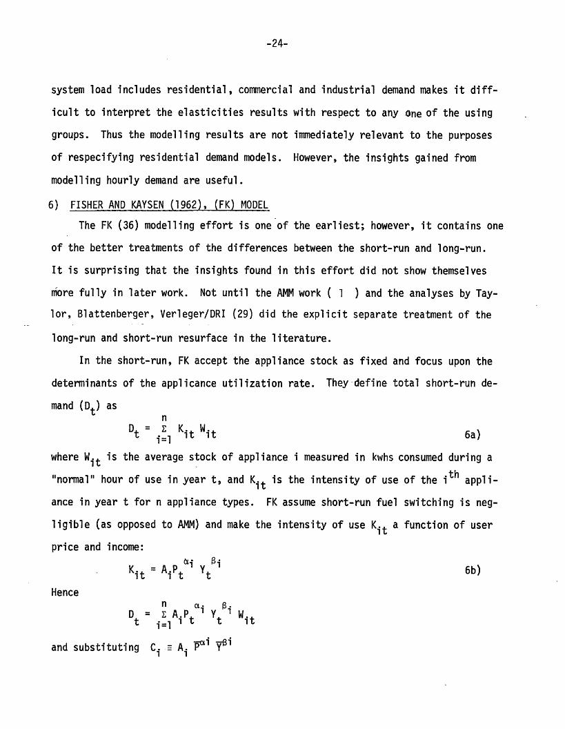
6) FISHER AND KAYSEN (1962), (FK) MODEL

The FK (36) modelling effort is one of the earliest; however, it contains one

of the better treatments of the differences between the short-run and long-run.

It is surprising that the insights found in this effort did not show themselves

more fully in later work. Not until the AMM work ( 1 ) and the analyses by Tay-

lor, Blattenberger, Verleger/DRI (29) did the explicit separate treatment of the

long-run and short-run resurface in the literature.

In the short-run, FK accept the appliance stock as fixed and focus upon the

determinants of the applicance utilization rate. They define total short-run de-

mand (Dt) asn

Dt = Kit Wit 6a)

where Wit is the average stock of appliance i measured in kwhs consumed during a

"normal" hour of use in year t, and Kit is the intensity of use of the ith appli-

ance in year t for n appliance types. FK assume short-run fuel switching is neg-

ligible (as opposed to AMM) and make the intensity of use Kit a function of user

price and income:

K AiPt Y 6b)it t t

Hencen as -

D z A P i Y Wt i=l t t it

and substituting C Ai i1 1

-25-

Dt = Z Cit ( t/ Wit 6c)

= C(Pt/P)~ (Yt/Y)B Wit 6d)

if "i = ' Bi = s, Ci = C for all i. Taking logs one obtains the FK basic equa-

tion

Dt = A' + aPt + Yt + Wt +t 6e)

nwhere primes denote logarithms, A = CP Y and Wt = Wit

If proper estimates of the weighted appliance stock (Wt) were available, 6e) could

be estimated. FK felt the data was not good enough; hence they assumed that Wt

grew exponentially in each state over the sample period. As a result, when taking

first difference in 6e), n Wt - An Wt_1 is constant and subsumed into A'. This

assumption seems to be too severe for all states; FK's analysis of the explanatory

power of the equation (R2) related to state's growth rate indicates that for the

fastest growing states, the assumption of simple exponential growth in Wt is least

supportable.

Estimating 6e) with assumed exponential growth in the appliance stocks for all

states over 1946-1957 using average revenue as the price specification yields price

elasticities that vary from -.03 to -.99 and income elasticities that vary from

.06 to .88 (when they have the correct sign.) In order to explain the differences

in these estimates, FK claim that greater urbanization is associated with greater

income and price elasticities, reflecting the stock of appliances in urban areas

and the more numerous substitutes available. When FK pool states by homogenous

regions based upon urbanized or rural characteristics, all elasticity estimates

become significant and e = -.16 to -.25 while ey = .07 to .33.

While some of FK interpretations as to the reasons why elasticities differ

-26-

across urban and rural, old and young states can be debated and seem contradic-

toryl, on the whole their elasticity estimates for pooled data yield short-run

elasticities estimates that corroborate such efforts as AMM; to wit ep = -.2

and ey .25.

For long-run demand, FK focus explicitly upon changes in the stock of con-

sumer appliances. FK first examine linear and logarithmic forms of the partial

adjustment model. However, they scrap the partial adjustment model because it

ideally models variables that exhibit the possibility of continuous variability

in the stock to desired levels (e.g. investment in all consumer durables). In this

case, the estimate of the partial adjustment parameter (O < x < 1) makes sense.

With appliance purchases by new households, the household either buys the new ap-

pliance or not; room for continuous variablity is lacking. In the face of these

difficulties (FK utilized a "disease model" relatina Wt/Wi - i.e. "spread:-ofit it-1

the disease") to the independent variables 2 as follows:

W. 'witj= A + il (I' - Y ) + li2't' + i2Yt 3Eit + ni4Git'

+ ni5(Ht - Ht-1 ) + ni 6(Ft - Ftl ) + ni7Mt' + hi8P 7)

+ ni9git + nilOV + Uit

where primes denote natural logs,

Wit -Wt = n (Wit/Witl) = the log of the change in appliance stocks

of type i for years t and t-l

Y ~t = seventeen-year moving-average of real personal income per

capita (Friedman's permanent income)

. . . . . . . . . . . . ..

1See pp. 29-60, where FK claim more urbanized states tend to have higher el-asticities while younger states also have greater elasticities.

2For full definition and data sources see FK (36), pp. 85-90.

-27-

Yt = current personal income per capita

Eit = electric appliance price

Git = gas substitute appliance price

Ht = number of customers per capita (i.e. customers/population)

Ft = population

Mt = moving average of marriages in t and t-l

= user cost of electricity (average revenue)

Yit = appliance efficiency, kwh consumption of appliance per hour of

average use

and Vt = three year moving average of gas prices.

FK find that net changes in appliances depend primarily on changes in long-run in-

come, population, the number of wired households per capita, and number of mar-

riages. Except for electric ranges and water heaters, the cost of electricity and

the price of the appliance have little effect upon stock demand. For washers and

refrigerators, economic variables are unimportant.

The apparent lack of importance of economic variables contradicts much of the

interfuel substitution literature. However, the contradiction is spurious. FK

find economic variables unimportant for washers and refrigerators where there is

little interfuel substitution; for these devices, current and permanent income,

population and number of wired households have the greatest explanatory power.

For ranges and water heaters greater possibilities for interfuel substitution ex-

ist and FK find the economic variables have greater explanatory power. If space

heating were analyzed I am sure FK would have found even better explanatory power

in the economic (own and cross operating prices and appliance costs) variables.

7) GRIFFIN (1974) MODEL

Griffin (37) develops a 25 equation, block recursive model of electricity sup-

ply and demand. For his residential demand specification he hypothesizes per cap-

-28-

ita consumption to be a function of capital stock per capita, income and fuel

prices. He estimates

DR K1 m YD n PR0N 1 N i =O i -iO i P 8)

where

DR is the total residential electricity demand

N is population

K1 is the stock of residential appliances (proxied by central air

conditioners)

YD is real disposable income

PR is the average residential electricity price

P is the GNP deflator.

Griffin also estimates per capita appliance stock as a lagged function of real

disposable per capita income. However due to data problems, he again models cap-

ital stock as central air conditioners alone.

Griffin finds that the short-run own-price electricity is -.06 and the long-

run elasticity is -.52. The respective income elasticities are .06 and .88. The

stock elasticity is .22 which is very small; it probably reflects the fact that

only central air conditioners are included in estimates of the appliance stock.

8) HALVORSEN (1973) MODEL

Few of the analyses summarized in Table 2 deal explicitly with the simultan-

eity difficulties inherent in modelling electricity demand. Halvorsen (38-42) at-

tempts to do so by specifying both supply and demand curves as follows:

Demand: Q = Q(P Y, Z, U) 9a)

Supply: Pm = P(Q, C, v) 9b)

-29-

where Q, the quantity demanded, is a function of marginal electricity prices (P ),

income (Y), and Z is a vector of other exogenous determinants. The supply/price

equation makes marginal electricity prices a function of quantity supplied and

costs of supply (C). v and u are disturbance terms. The factors that Halvorsen

includes in Z are price of gas, price of electric appliances, percentage of pop-

ulation living in rural areas, number of heating degree days, average size of

households, average July temperature, percentage of housing units in multi-unit

structures. Halvorsen estimates the structural equations 9a) and 9b) and reduced

form equations with various lag structures. He finds that the static model works

as well as the dynamic model, and utilizes the static formulation for most of the

analysis. However his tests upon the static versus dynamic character of the model

are based upon 1961-1970 data when the independent variables were smoothly trending.

Similar experiments based upon 1970-1975 experience would more conclusively deter-

mine the relative performance of the static and dynamic models' predictive power.

Halvorsen's structural demand equations are credible; however, the supply/

price equation is relatively ad hoc and poorly specified. As a result, elasticities

estimated from the demand equation appear to be believable; however, total system

elasticities based upon 9a) and 9b) are suspect given difficulties in the estimated

supply/price relationship. Demand elasticities from the structural demand equation

indicate statistically significant long-run own-price elasticities of -.049 to -:088

and income elasticities of .47 to .54. These estimates differ for regionally pooled

data. In various regions, household size, July temperature and time become sign-

nificant. The use of marginal and average electricity prices yield very similar

elasticity estimates. Halvorsen uses nominal prices, which is a problem.

9) HOUTHAKKER (1951) MODEL

Houthakker's analysis (54) focuses upon a cross-section of 42 provincial towns

in the United Kingdom for 1937 and 1938 using the equations

-30-

X = aM + b/P + cq + dh + 10a)

and In X = aln M + ln P + yln q + 61n h + ' lob)

where

X is average annual electricity consumption per customer on a 2 part

tariff

M is average money income

P is marginal price of 2 part tariff

q is marginal price of gas on domestic tariffs

h is customer holdings of heavy domestic equipment

Gas and electricity prices are lagged 2 years to avoid simultaneity problems.

This specification is similar in spirit to AMM and FK in that appliance stocks

are held constant and short-run demand is predicted on the basis of prices and in-

come. The estimated short-run elasticities are: ey = 1.17, ep = -.89, eq = .21,

and eh = .18, which are high when compared with other studies. The higher price

elasticities may reflect the fact that prices are lagged two years; hence the elas-

ticities are closer to long-run estimates.

10) HOUTHAKKER, VERLEGER, SHEEHAN (1974), (HVS) MODEL

The HVS model (56) differs from the previous models in that it does not ex-

plore a wide array of independent variables. It utilizes only electricity price

and income in a flow adjustment formulation. Thus, HVS define desired equilibrium

consumption Qit* to be

.Y 31a)Qit* = it it Yitla)

while the adjustment mechanism is

Qit/Qit-l = (Qit*/Qit-l) 1 lb)

Hence, HVS obtain

In Qit = lna + oYlnPit + oelnYit + (l-o)lnQitl

HVS utilize a pooled time-series of cross-sections for states from 1961-1971. They

-31-

utilize an error components technique which allows for a state component in the

error term. The use of the state error component corrects for differences across

states that are not included in the price and income effects. HVS use three dif-

ferent price specifications: the differences between typical electric bills (TEB)

for 500 and 100 kwh, 250 and 100 kwh and 500 and 250 kwh. The elasticities re-

sulting from these price specifications are listed in Table 2. For the first two

prices, low short-run elasticities and long-run elasticities of about -1.2 to -1.6

result. For the third price specification, similar short-run elasticities are es-

timated; however the long-run price elasticity estimate is much lower. The 500

and 250 kwh difference is the most relevant of the three price variables; hence,

the lower long-run elasticity estimate of -.45 must be taken seriously.

In a thorough examination of the HVS model, Charles River Associates (25)

found similarly small long-run price elasticities for equations utilizing the 500-

250 kwh TEB. However, for the price variable expressed as the difference between

TEBs for 1000 and 500 kwh, the long-run price elasticity is estimated to be -1.085

and the long-run ey = .63. These estimates are much closer to the static equilib-

rium model estimates of Halvorsen and Anderson. In spite of its simplicity, the

forecasting and backcasting performance of the HVS model is shown in the CRA work

to be quite good, when actual values of the lagged endogenous variable are used.

11) MOUNT, CHAPMAN AND TYRRELL (1973), (MCT) MODEL

MCT (68) model the residential, commercial and industrial sectors individually.

They utilize a flow adjustment model with a lagged endogenous variable. Further-

more, in addition to the usual constant elasticity model specification, MCT specify

a variable elasticity model. The constant elasticity model (CEM) is:

Q =A it-i lit VNit 12a)

where i is the state

t is the year

-32-

Q is the quantity of electricity demanded

Vn is the level of the nth causal factor

In the partial adjustment formulation, the short-run elasticity (eSR) of Q

with respect to Vi is Bi and the long-run elasticity (eLR) is i/(l-X). The two

variable elasticity models are

81 YN ¥1/V 1 it ¥N/VNi tQ V e 12b)it AQit-1 lit e b)

andAeo/Dt 1 l+61/Dit Vl +Nlj /Dit e it

Qit Ae it-1 Vlit VNit

YN/VNit 12c)...e

where all the variables are defined above and D is a demographic/geographic shift

variable. For 12b) eSR = (i - Yi/V) and eLR =(i - yi/Vi)/(l-x). For 12c),

eSR = [i - (yi/Vi) + (i/D)] and e LR = eSR/(l-X). These variable specifications

permit elasticities to vary with region (i.e. demographic/geographic values for D)

and with levels of the independent variables (e.g., if income elasticities vary

with y Vkt, then yk/Vk 0). MCT utilize OLS and instrumental variables (IV)

techniques in estimation. Their price specification is average price. Their in-

dependent variables are real personal income per capita, gas price measured as av-

erage revenue, price of appliances of machinery, mean January temperature and pop-

ulation. They estimate the equation in log-linear form.

The long-run estimates for both OLS and IV techniques are quite similar; the

short-run estimates differ considerably. Since eLR = eSR/(1-X), the reason is that

the estimate of the partial adjustment factor is lower in the IV case while the

short-run elasticity estimates are higher. The elasticity estimates in Table 2

are OLS results. The long-run own price elasticity is -1.2. This estimate holds

for the constant and variable elasticity models, for the OLS and IV estimates.

-33-

The long-run gas cross-elasticity is .2, while the income elasticity is .21. The

respective own-price, gas cross-price and income short-run elasticities are (-.14

to -.36), .02 and (.02 to .10). Thus the estimated short-run OLS elasticities are ex-

tremely small. The IV estimates are more believable because they are statistically

consistent. As stated above, the long-run IV estimates are similar to those in

Table 2. The short-run IV estimates are about twice as large; hence, they are

still inelastic. Overall, in the long-run electricity demand is price elastic

and increasingly so as prices rise. Demand is income inelastic and increasingly

so as income rises. Demand is unitarily elastic with respect to population.

12) MOUNT AND CHAPMAN (1974), (MC) MODEL

Utilizing a similar modelling approach, MC (68A) examine alternative price

specifications for residential electricity demand. The resulting elasticity es-

timates are quite similar to those found in MCT except for the income elasticity

estimates which are somewhat larger.

13) TAYLOR, BLATTENBERGER, VERLEGER/ DRI (1977), (TVB) MODEL

TBV (29) analyze residential energy demand at three levels: demand for gas,

oil and electricity by state; demand for appliance services through appliance stock

utilization rates; and demand for appliances. TBV deal with the differences be-

tween short-run and long-run consumer behavior similarly to Fisher and Kaysen: they

distinguish between short-run demand as a choice of the capital stock utilization

rate and long-run-demand as a choice of the size and characteristics of the appli-

ance stock. As with the Acton, Mitchell and Mwill analysis, TBV deal explicitly

with the consumer theory of demand functions in the face of declining block tar-

iff schedules. They utilize as a result both a marginal price and inframarginal

fixed charge in fully articulating the budget effects of electricity rates.

For means of comparison TBV introduce the flow adjustment model utilized to

explain energy demand similar to that of Houthakker and Taylor (55):

-34-

qt= e(q - qt) 13a)

with

qt = a + alXt + 12t + 3Zt 13b)

and therefore

t a= 0e - oqt + aleXt + a2ewt + a3ozt 13c)

where q is the amount of electricity (or natural gas of fuel oil) consumed, x is

income, is price (for electricity, consisting of a marginal and a fixed compon-

ent) and z is a vector of other exogenous factors.

The appliance stock utilization models are of the form

q = u(x, , z)S 13d)

where the utilization rate of applicance stock S is a function u of x, , and z

as defined above. Whereas the flow adjustment model in 13a) - 13c) do not explic-

itly deal with the characteristics and size of the appliance stock, the model in

13d) assumes that the appliance stock is given in the short-run. The utilization

rate is a function of current variables. Utilization rates for subgroups of ap-

pliances can also be examined:

q = ul(x, , Z)S1 + ... + um (X,, , )Sm

Equation 13d) can also be expressed and estimated as

q/S = u(x, , z) 13e)

Equation 13d) requires aggregation of appliance stocks. Fisher and Kaysen

utilized "normal use" as weights. TBV do the same so that

nS t = Z W i Sit

i=l

where Sit is the stock of the ith type of appliance and w is the weight where

UiWi = *

J

-35-

* 1and u denotes the "normal" utilization rate of the ith appliance.

To complement the stock utilization models, a model of capital stock accumu-

lation is required. TBV define equilibrium appliance stocks S to be

S = + 1 x + 2 + B3(r + )P + 4z 13f)

where x, fW and z are defined above and r is the market rate of interest, 6 is the

depreciation rate of the appliance stock and P denotes the per watt price of ad--

ditions to the appliance stock. Hence, (r + s)P is a user cost of capital services

per watt. Combining 13f) with an assumption about replacement investment and the

partial adjustment formulation that new investment = (S* -S), TBV obtain 1

Y = + BX + B2 + 3(r + 6)P + q4z + (a - g)S 13g)

where y is gross investment in appliances.

Equations 13d) and 13g) are the explicit short-run/long-run dichotomization

of the simultaneous consumer decisions that are subsumed into the usual partial

adustment or flow adjustment models.2 The partial adjustment and flow adjustment

models yield similar elasticity estimates in the log-linear specification; the

first row of TBV elasticity estimates in Table 2 are those from the flow adjustment

model utilizing in addition to x and , the price of natural gas, heating degree

days, and cooling days in z. The resulting own-price elasticities are -.82 and

-.08 in the long-run and short-run. The elasticities with respect to the fixed

electricitycharge are -.17 and -.02 in the long-run and short-run. The income el-

asticities are .10 and 1.08 in short-run and long-run.

The second and third rows of elasticity estimates in the TBV analysis results

refer to the capital stock equations 13e) [or 13d)]and 13f). x, wr and z are defined

lSee Taylor, Blattenberger, Verleger/DRI (29)for details.

2To be precise, the flow adjustment and partial adjustment models differslightly in their specification. They are compared fully by TBV(29) chapter 5.

-36-

as above.

The short-run own-price elasticities vary from -.06 to -.54 depending upon

the specification of 13e). Since not all the equations were estimated in a dy-

namic form, it is difficult to ascribe long-run elasticities for each of these

short-run estimates. A reasonable bound is -.12 to -1.0. The cross-price elas-

ticity estimate is nearly zero; hence there seems to be little interfuel substitu-

tion in the short-run, a fact assumed by Fisher and Kaysen and found by Anderson.

The capital stock equation 13f) is estimated for refrigerators, freezers, room air

conditioners, water heaters, stoves, automatic washers, conventional washers, dry-

ers, central heating and central air conditioners. The own-price (marginal price)

elasticity estimates vary from -.02 to -.22. The cross-price elasticity estimates

vary from .02 to .10. Income elasticity and user capital charge elasticity esti-

mates vary widely for the different appliances analyzed.

Long-run elasticities of energy use can be estimated by assessing the total

effect of changes in the independent variables upon appliance stocks and utiliza-

tion rates:

aq z _ i zaz q z (q/s) + w az S*

i ~1

where q is energy sales and the other variables are defined above (I use z as a

generic independent variable here, including marginal price or income). It is

interesting to compare these total elasticity estimates with the long-run consump-

tion elasticities that are generated by the usual partial adjustment specifications.

Depending upon the specification for 13e),TBV find long-run sales elasticities of

income to be 1.00 - 1.30 and own-price (marginal) elasticities to be -.46 to -.90.

The mean estimates are ey = 1.20 and ep = -.60. Such estimates accord with sev-

eral long-run elasticity estimates (Anderson, HVS, MCT) from the single equation

-37-

partial adjustment models; however they are based upon explicit analysis of short-

run and long-run behavior.

14) WILLIS (1977) MODEL

Wills (87) utilizes a short-run demand model similar to the Taylor, Blatten-

berger, Verleger/DRI (TBV) capacity utilization model 13d) and the Fisher and Kay-

sen (FK) model. Wills also utilizes both marginal prices and fixed charges for the

declining block rate tariff schedules as done by TBV and Acton, Mitchell and Mo-

will. Wills tried a number of specifications; the specification for which he re-

ports results is,

q = + 1PM + 2Y + 3 PSFD + a4 HEAT + a5 WATER

+ a6 STOVE + 7 COLOR TV + a8 FROST 14)

where all variables are in logs and

q = kwh consumed/month/household

PM = marginal electricity price

Y = income

PSFD = percentage of customers living in single family dwelling

HEAT = a dummy variable, equal to one if consumption is in an all-elec-

tric rate and zero otherwise

WATER = a dummy variable, equal to one if consumption is on a rate dis-

counted for owners of electric water heaters and zero otherwise

STOVE = per single family dwelling ownership of electric stoves

COLOR TV = per single family dwelling ownership of color televisions

FROST = per single family dwelling ownership of frost-free refrigerators

The coefficient for the fixed consumer charge was never significantly different

from zero; as a result, Wills subtracts the fixed charge from income and uses the

the resulting net income as Y in the equation 14). The variables included in the

*�W�D�MI�:�*'Y*rJnrX�*�rr;�u�'rrrr;r�r, r^-- 1-I---��-I·^··----- ·--·- -------- -

-38-

regression are clearly extremely disaggregated and refined; they result from con-

sumption data for 39 Massachusetts electric utility districts and 57 residential

rate structures. The short-run elasticity estimates conform with those of TBV and

FK: the short-run own-price elasticity is -.08 while the short-run income elas-

ticity estimate is .32.

A number of questions still remain for the Wills work. When HEAT and WATER

are excluded, the explanatory power of the^regression falls considerably and the

coefficient estimates of PM and Y reverse signs. When saturation rates are used

for space heating and water heating, the own-price elasticity is -1.33 which is

unacceptably large. Further effort is required in assessing the usefulness of

these dummies and saturation rates in capturing the presence of the appliance

stock because they provide a simple substitute for the weighted appliance stock

estimates used by TBV and FK. Those estimates utilize weights based upon "normal"

usage; the problem is that normal usage will change with the independent variables.

The utilization of saturation rates would avoid this difficulty.

15) WILSON (1971) MODEL

The Wilson model (85-86) focuses upon residential electricity demand and de-

mand for six categories of household appliances. In the electricity model, 77

cities in 1966 provide the cross-section; 83 SMSA's in 1967 are used for the ap-

pliance demand. The electricity demand is reported herel; it is given by

Q b + b2P + b3G + b4Y + b5R + b6C + 15)

where

Q is the average electricity consumption per household

P = price of electricity (TEB for 500 kwh/Mo.)

1The appliance modelTing corroborates other efforts. The own price elasticityis significantly negative and' less than -1 for all but home freezers. The priceof natural gas is important in the equations for ranges, water heaters, and dryers.

i*r�h�-glg,�gna*d�E�rr^Ria·�r�l�;lOT.rlu p..xrxr n----rr C_-a;rl--arr^�-.- r --- ----- -----̂ -·_

-39-

G = average gas price (cents per therm)

Y = median family income

R = average number of rooms per household

C = number of degree days

The estimated elasticities are ep = -1.33, eG = .31 and ey -.46. All are sig-

nificantly different from zero. The own-price elasticity is quite large at -1.33

even for a long-run elasticity. The income elasticity is the wrong sign; it makes

one wonder about the other estimates.

16) SUMMARY

In the early discussion of this section, three consumer decisions were iden-

tified for energy demand:

* The consumer decides whether to buy a fuel-burning consumer durable, ca-

pable of providing a particular consumer service (e.g. cooking, heating,

lighting, air conditioning etc.)

* The consumer decides on the characteristics of the equipment he desires,

including efficiency, technical characteristics and fuel type to be

burned.

* Once the equipment is acquired, the consumer decides on the frequency and

intensity of use.

These three decisions span short-run and long behavior.

A number of modelling techniques have been utilized to deal with one or all

of these decisions. Three techniques predominate in the analysis reviewed above.

They are:

* Static long-run equilibrium formulations

* Dynamic partial adjustment of flow adjustment formulations

* Explicit multi-equation analyses of appliance stock utilization and

changes in the appliance stock.

The models reviewed that are static, long-run equilibrium formulations include

-40-

those of Anderson (5,6), Halvorsen and Wilson. The dynamic partial or flow ad-

justment formulations are found in the analyses of Anderson (6); Balestra; Houth-

akker, Verleger, Sheehan; Mount, Chapman and Tyrrell; and Taylor, Blattenberger,

Verleger/DRI. Analyses that focus explicitly upon short-run demand (given fixed

appliance stocks) and/or long-run demand (through appliance stock changes) in-

clude those of Acton, Mitchell and Mowill; Fisher and Kaysen; Griffin; Houthakker;

Wills: Taylor, Blattenberger, Verleger/DRI; and Cargill and Meyer.

The theoretical specification and the empirical implementation of the fif-

teen models have been discussed briefly above. Some comparative and critical

comments were provided; however, greater critical review is required along the

lines of the eight criteria of evaluation introduced in Section B. The follow-

ing discussion critically summarizes and reviews the modelling efforts utilizing

the eight model assessment criteria.

i) Proper identification of major market participants and the level of dis-

aggregation required.

All of the models reviewed analyze electricity (gas and oil where appropriate)

demand at the residential level except for Balestra who aggregates commercial and

residential demand and Cargill and Meyer who aggregate the commercial, residen-

tial and industrial sectors. Such aggregation is inappropriate if one is inter-

ested in the residential sector specifically, given the data that is currently

available. Usually total energy demand is analyzed on an annual or monthly basis.

Either basis is appropriate; however the more temporally disaggregated the data,

the better. Those analyses which deal with utilization of or changes in the ap-

liance stock disaggregate residential stocks into a number of fuel-use categories

including combinations of refrigerators, freezers, room air conditioners, water

heaters, stoves, automatic washers, conventional washers, dryers, space heating

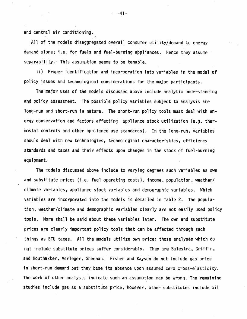
-41-

and central air conditioning.

All of the models disaggregated overall consumer utility/demand to energy

demand alone; i.e. for fuels and fuel-burning appliances. Hence they assume

separability. -This assumption seems to be tenable.

ii) Proper identification and incorporation into variables in the model of

policy issues and technological considerations for the major participants.

The major uses of the models discussed above include analytic understanding

and policy assessment. The possible policy variables subject to analysis are

long-run and short-run in nature. The short-run policy tools must deal with en-

ergy conservation and factors affecting appliance stock utilization (e.g. ther-

mostat controls and other appliance use standards). In the long-run, variables

should deal with new technologies, technological characteristics, efficiency

standards and taxes and their effects upon changes in the stock of fuel-burning

equipment.

The models discussed above include to varying degrees such variables as own

and substitute prices (i.e. fuel operating costs), income, population, weather/

climate variables, appliance stock variables and demographic variables. Which

variables are incorporated into the models is detailed in Table 2. The popula-

tion, weather/climate and demographic variables clearly are not easily used policy

tools. More shall be said about these variables later. The own and substitute

prices are clearly important policy tools that can be affected through such

things as BTU taxes. All the models utilize own price; those analyses which do

not include substitute prices suffer considerably. They are Balestra, Griffin,

and Houthakker, Verleger, Sheehan. Fisher and Kaysen do not include gas price

in short-run demand but they base its absence upon assumed zero cross-elasticity.

The work of other analysts indicate such an assumption may be wrong. The remaining

studies include gas as a substitute price; however, other substitutes include oil

-42-

and coal. Only Anderson (1973) includes these substitute prices. Furthermore

although all studies include own-price, only Acton, Mitchell and Mowill; Taylor,

Blattenberger, Verleger/DRI; and Wills explicitly deal with the declining block rate

tariff structure through a marginal price and a fixed charge. The remaining aal-

yses use average price, or TEB. This treatment of marginal and fixed charges

will permit analysis of proposed electricity rate restructuring proposals such

as rate leveling and rate structure inversion. Finally, none of the studies

deal with the need for articulating gas prices through'both a marginal rate and

fixed charge. This absence introduces potential misspecification and biases the

long-run gas price cross elasticity to zero. It also limits policy analysis of

rate restructuring for gas prices.

The presence of an income variable provides a limited policy tool. However

greater analysis of appliance stock characteristics (efficiency., uncertainty of

new technologies) and appliance capital costs are required in both the long-run

and short-run. In the long-run, technological characteristics of old and new

technologies and the cost of capital services must be taken into account. Fisher

and Kaysen (FK), Mount, Chapman and Tyrrell (MCT) and Taylor, Blattenberger, Ver-

leger/DRI (TVB) do include appliance prices; however, there exists interfuel com-

parison of technological characteristics which is crucial for long-run appliance

stock demand by fuel-use category. In the short-run, the capacity utilization

models of TBV and--AMM utilize "normal" use to aggregate appliance stocks; changes

in such normal use can be utilized in an ad hoc fashion to assess attractive con-

servation policies. However, explicit treatment of appliance stock efficiency is

also needed to properly handle short-run demand and short-run policy possibilities.

Finally, some policy proposals such as peak load pricing options require

See Taylor, Blattenberger, Verleger/DRI (29).

-43-

seasonal and daily demand modelling. Few models have achieved that level of re-

finement. Acton, Mitchell and Mowill utilize monthly data and could be used to

investigate changes in load duration curves on a seasonal basis. The model of

Cargill and Meyer assesses hourly electricity demand and could be utilized to

analyze the effects of hourly peak load pricing.

iii) Proper degree of geographical dlsaggregation

For the purposes of most policy analysis and simulation experiments, disag-

gregation to state level is sufficient. Most of the models in Table 2 are disag-

gregated to that level. More detailed and refined analytic results and policy

assessments are possible if the geographical units are utility areas, meter read-

book areas, cities and SMSA's (such as the works of Acton, Mitchell and Mowill,

and Wills).

iv) Utilization of the appropriate behavioral models and underlying behav-

ioral assumptions

As stated in the beginning of this summary, three sets of models have been

utilized to deal with the short and long-run consumer decisions involved in en-

ergy demand. They include static equilibium models, dynamic partial (flow) ad-

justment models and multi-equation separate treatment of the long-run and short-

run. The static and dynamic models treat energy demand in aggregate without ex-

amining the relationship of such demand to the underlying fuel-burning appliance

stock. The models implicitly assume some long-run equilibrium relationship of

fuel demand to appliance stock, where both the fuel demand (stock utilization)

and the stock are related to combinations of P, PS' Y, N, W, A, D and t in Fig-

ure 2. This is clearly a difficulty when potential policy actions and economic

factors will affect appliance stock utilization rates.

Within this group of model types, the static equilibrium models (Anderson,

Halvorsen and Wilson) are not designed to track short-run time series variation.

-44-

Anderson experiments with both dynamic and static formulations and finds that due

to the relatively steady-state trending of the important variables in the 1960's,

either the static or dynamic versions of demand models provided essentially the

same parameter estimates and simulation performance. However this will not be

the case for periods when such smooth trending in the economic time series is

lacking, such as the 1970's. To take account of short-run disequilibrium effects,

the dynamic models utilize lagged consumption. These models include Anderson

(1973); Balestra; HVS; MCT; and TBV. By including the inertial effects of past

consumption upon current consumption, these partial (or flow) adjustment models

are definite improvements upon the static equilibrium formulation. Since energy

demand is characterized by three consumer decisions (see overview of this section)

that combine short-run and long-run behavior, the partial adjustment formulation

permits explicit differentiation of the long-run and short-run responses.

In spite of the improved theoretical specification in the dynamic adjustment

models, more explicit differentiation between and delineation of the determinants

of long-run and short-run demand is required. The dynamic adjustment models

still ignore the relationship of capital stock to fuel demand; they impose a con-

stant relationship between the short-run and long-run elasticities for all exog-

enous variables (eLR = eSR/l-X); they still do not permit explicit identification

of long-run and short-run policy variables. The appropriate approach is explicit,

separate multi-equation treatment of the long-run and short-run as found in AMM,

FK, TBV, and Wills. Although each of these particular analyses has its own dif-

ficulties in terms of data and variable specification and/or exclusion, the group

does represent the properly dichotomized behavioral specifications. The TBV an-

alysis compares the long-run and short-run elasticities that result from a par-

tial adjustment model and from a combined capacity utilization/capital stock model;

the elasticities are not widely divergent. However, the combined multi-equation

-45-

analysis is much more refined in terms of data used and much more sound in terms

of explicit behavioral representation and inclusion of policy variables.

v) Proper integration of the demand analysis into an overall energy and/or

macroeconomic model

This criterion is appropriate for demand analyses that are part of a general

equilibrium model. Most of the models reviewed here (except for Griffin) are

not a part of larger models; hence, issues of proper integration and/or problems

arising form improper integration are not relevant. In terms of using any of

the models, all would require a set of assumptions about the exogenous variables

in which the models are set. The more refined and complicated the model, the

greater are the exogenous data requirements.

vi) Utilization of the proper data and statistical econometric techniques

This criterionproves to be a thorny one, particularly with respect to appro-

priate data. The appropriate statistical/econometric techniques are usually

2SLS, instrumental variables (IV), GLS, and/or an error components model. How-

ever in some cases', OLS has been used in generating results not widely different

than those from a consistent technique (e.g., Mount, Chapman and Tyrrell long-run

elasticities). Parameter estimation in the presence of serial correlation and a

lagged endogenous variable is dangerous. If consistent techniques (IV, 2SLS)

are not used, the parameter estimates can be worthless. Furthermore, even if

consistent techniques are utilized the parameter estimates, particularly of the

lagged endogenous variable, are extremely sensitive to assumed stochastic spec-

ification, sample period definition and variable definition.

It was not possible in this effort or in the original model-building efforts

to subject these models to rigorous testing including forecasting, backcasting,

estimation for sub-categories of data to test parameter estimate robustness, and

examination of alternative variable specifications. TBV did some such analysis

-46-

by assessing the effects of different price specifications (marginal and fixed

charge versus average revenue). They found little difference among them. How-

ever, Charles River Associates (CRA) subjected the Anderson, Halvorsen, HVS, and

MCT models to rigorous model assessment along these lines. Their conclusions are

disquieting. In the first place, CRA found little parameter robustness. Slight

changes in the estimation period and definition of variables leads to widely dif-

fering parameter and elasticity estimates. For example, HVS generates price elas-

ticity estimates which double as they move from one typical electric bill (TEB)

to another. Likewise when CRA estimates the Anderson model for different regions

to correct for regional differences (such as the presence of cheap electricity

in the Pacific Northwest and TVA regions) the pri.ce elasticities fall from -1.3

to -.5. Secondly, CRA feels the long-run price elasticity is overstated in these

four models for the following reasons: a) the problem of identification and spec-

ification of the rate structure bias the own price coefficient away form zero ;

b) aggregation of end use and cross-sectional (location/regional) variation

overstate elasticities; c) gas and electricity price elasticity estimates are not

consistent; d) a price elasticity greater than 1-1.01 cannot be plausibly explained

in behavioral terms in light of realistic changes in the stock of consumer dur-

ables; and e) industry people claim that leLR I < 1.

These criticisms are aimed particularly at the static and dynamic adjustment

formulations. The greater data refinement and disaggregation by end-use and bet-

ter behavioral specifications inherent in the multi-equation capacity utilization/

capital stock formulations of AMM, FK, and TBV avoid some of the difficulties.

lIt is therefore interesting that when TBV estimate the long-run price elas-ticity utilizing the theoretically correct two-part tariff specification withthe usual partial adjustment model, they obtain an estimate of -.82 (see Table 2).

-47-

However one must still be careful to correct for cross-sectional variations (based

upon climate, gas availability, regional availability of electricity in TVA and

the Pacific Northwest) that will overstate elasticity estimates. Likewise one

must attempt to avoid misspecification by dealing with the marginal and fixed

charges inherent in the declining block rate tariff structures for gas and elec-

tricity.

vii) Provision of good documentation for the use of the energy demand

modelling

viii) Provision for relatively easy accessibility and extensibility of the

modelling effort

All 15 models score well under these two criteria. The data sources util-

ized by the analyses are usually well documented; alternative variable specifi-

cations and parameter estimates are presented.

Throughout the preceding discussions, the need is apparent to utilize the

appropriate behavioral specifications, data, variables, and econometric/stat-

istical techniques in order to properly analyze and quantify consumer response

and behavior. Table 3 summarizes the resulting measures of consumer response

for 14 models. For electricity demand, own-price long-run elasticity estimates

vary from -.52 to -1.33. The largest estimates are those of Halvorsen, Wilson,

Anderson (1973) and MCT. When TBV utilize a better price specification, the

elasticity bias away from zero is eliminated somewhat and ep = -.82. The AMM

and TBV analyses of capacity utilization indicate lower long-run elasticities,

-.12 to about -1.0. The short-run elasticities are generally much lower whether

measured by a partial adjustment model (HVS) or by explicit capacity utilization/

capital stock models (AMM and TBV). The cross-elasticity estimates indicate rel-

atively uniform severe inelasticity, except for the estimates of AMM in the short-

run. This is disquieting because AMM seems to have the best data and the theor-

a)aiCO

r-q

O 0

P4

H0o

a) a)o CKOO H

I c I

4-J 4-Jql X-)u u

I I I'

EnX ;l - 00Cl

0

o

'IO

*It

C!

H o C*-i * r

Un 00 C') Ln I-

I I ICr)~~~~~

* O H 00 C* - .00 -

i ; I I I

o0

o4i

H-

OH H.

0co 4'-It00 Lr)

I.

0

Cl4

o

oo ·4.Lr C

0

O 04J00 4.. U)

I°

* .0

I

O

H H 00'D Cl '0 0

r; r;O

04i

%DHH)0lr

o% 0U O O O" 0 c)

o H I - I. II I

0

·o~Cl 4-J CI . I

U4.J

N- CI Cl4OO C H 00 H A* * * H: 4 - H IIII I I

ao

P va) .-I

F41

i 4-1 . ia) oCb4 H

LH _

o H H

44 0 , = c)4- > U

Cd tr 0 0

^

Y v, D Ej'l C10 UI 0r. r r l

co 1 coH tX4) a)- 4 -i-,1

w - T0. P- O Hr

: H P '- -'

I a)4-IJ )

-q 9 r-dN

E-,a I

H I Cl C - UL '0 - 00 (O 0 H CCl

r-N-

.r-I

I

r-

H3

- -'rC',i -1IH Ht

a)

a44-)coH

HClpqP0r-I

E-x

w

r4a)od0

oo

O0

4.1

CUC)

r

a)00

C)

0z

14a)

E-,

uC/

-48-

en 0o

o

0O

o 00

o

0C-)z

U

P-)H

InI

0C.,u

C)

*10

ri)Hot

V)

H

V0

HHC-,HuH

C-,

H

H

C-)

iu

04- o

.l

0

lt)a)0

o

o

04~i

r-icl e''.

0

wuC-)

H4II

I'c1.

4-)

U);j

H.,r--fCY) I~

r4Cd

.rq4-Ju

a)

acor-iP(1)

* >

.r- W

0 04. 4J

00 -o I

I * II I

00o

r.

a)d v

I

ca)C).14

oCO3

T$ar

hU)

oNC, a

cd_ H

¢ I co H0la) bo

uc I

-49-

etical specification of short-run demand. Such a large estimate of short-run

cross-price response seems implausible but merits further investigation. The in-

come elasticity estimates vary from the improbable short-run estimates of 1.17

of Houthakker to the even more improbable long-run estimate of -.46 of Wilson.

The partial adjustment estimate of TBV seems most believable.

The consumer responses to own and substitute prices summarized in Table 3

need to be complemented by response estimates to weather, fuel (gas) availability,

capital stock prices and characteristics and policy variables. Such response

estimates must result from the further analysis proposed in Section E.

-50-

D) INTERFUEL SUBSTITUTION DEMAND MODELS

Using the criteria of Section B in order to evaluate their ability to prop-

erly analyze both the nature of demand (in the short-run and long-run) and the

competitiveness of new technologies, the individual fuel demand models introduced

in Section C were found to exhibit varying degrees of sophistication with respect

to behavioral specification, refinement of data and variable definition, utili-

zation of econometric/statistical techniques and the inclusion of policy options

and technological characteristics. One problem with all of these models, however,

is that the possibilities for and effects of interfuel substitution are not ex-

licitly examined. The models contain a number of cross-elasticities. However,

to fully examine the long-run determinants of energy demand for all fuels, to

explore the potential for market penetration of new fuel-burning technologies

against each traditional fuel-burning technology and to adequately assess the

desirability of each fuel in comparison with its potential substitutes, a model

of interfuel substitution is required. The major premise of such interfuel sub-

stitution models is that the desirability (i.e. demand for) of any given fuel

cannot be understood or predicted without explicitly predicting and understanding

its desirability relative to all possible competitive fuels.

Five interfuel substitution models are examined here. They are:

* The Baughman/Joskow (BJ) Model

* The Federal Energy Administration Project Independence EvaluationSystem (FEA/PIES) Model

* The Oak Ridge/Hirst et al. (OR/H) Model

e The Anderson Model

e The Erickson, Spann and Ciliano (ESC) Model

The B/J and FEA/PIES models are more general equilibrium in their purview, modelling

demand by all using sectors in addition to supply and market clearing. Only the

demand modules of these models will be discussed in any detail here. The remaining

-51-

three models analyze demand alone.

The discussion here will proceed by introducing the models (or demand modules

thereof). As in Section C, the critical summary will then summarize the evalu-

ation of these models by the criteria introduced in Section B.

1) THE BAUGHMAN/JOSKOW (B/J) MODEL

The B/J Demand analysis is a module in the B/J Regional Electricity Model

which also includes a Supply module and a Financial/Regulatory module. While

all fuel types (coal, oil, gas and electricity) are examined, the principal focus

of this model is the electric utility industry.

The energy demand module of the B/J Model consists of two major sectors:

the residential/commercial sector and the industrial sector. I shall introduce

them in some detail because the structures of several other interfuel substitution

models are similar. The basic structures of these two sectors are presented in

Figures A and lB. Figures 2A and 2B present the equational specification of

the sectors.

The energy demand behavior assumed in both sectors is step-wise rather than

simultaneous; the behavioral specification begins with aggregate energy demand

and then disaggregates it into state demand (for industrial) and particular fuel

demands (for commercial/residential and industrial). The model of consumer be-

havior for the commercial/residential sector is summarized by B/J in [Baughman

Joskow (13) p. 306]: "The consumer decision-making process is composed of two

steps. First the consumer decides on a level of energy-using services that he

desires based on the price of energy, the prices of other goods and services and

household income. This decision defines the expected level of energy that will

be consumed. The consumer then seeks to find a combination of fuels that will

provide these services most cheaply."

The decision model for the industrial sector is separated into three decisions

-52-

FIGURE 1A : BAUGHMAN/JOSKOW DEMAND MODULE

RESIDENTIAL AND COMMERCIAL SECTOR

N/

ESTIMATION OF TOTAL ENERGY

DEMAND PER CAPITA BY STATE

DISAGGREGATION OF TOTAL

ENERGY DEMAND INTO DEMAND

FOR PARTICULAR FUELS

(GAS, OIL OR ELECTRICITY)

i l m , , , , , , , ,

I | --- --- -

h

-53-

FIGURE 1B : BAUGHMAN/JOSKOW DEMAND MODULE

INDUSTRIAL SECTOR

AGGREGATE DEMAND FOR

ENERGY IN THE

UNITED STATES

I

LOCATIONAL DECISIONS ON THE

PART OF INDUSTRY

DISAGGREGATION OF TOTAL

ENERGY DEMAND INTO

DEMAND FOR PARTICULAR

FUELS (GAS, OIL,

ELECTRICITY, COAL)

I

. I

I I

-54-

FIGURE 2A: RESIDENTIAL AND COMMERCIAL SECTOR, EQUATIONAL

SPECIFICATION

GAS GAS PRICE~~~~~~~~~~~

GAS GAS PRICE)=A+C* LOG (LOGELECTRICITY LOG ELECTRICITY PRICE)

+D* (MAXIMUM TEMPERATURE)

+F* (MINIMUM TEMPERATURE)+H* LOG GAS EL IT(-1)ELECTRICITY (-1))

OILCT OIL PRICEELECTRICITYLOG ELECTRICITY PRICE

+ E* (MAXIMUM TEMPERATURE)

+G* (MINIMUM TEMPERATURE)+H LOG OELETRICITY (-))

RANGE =1968 - 1972 R2 = 0.954 F(7/482) = 1462

COEF VALUE T-STAT

A 0.07 0.568 0.208 1.65C -0.137 -3.29D -0.0015 -1.04E -0.0022 -1.58F -0.0022 -1.74G -0.0063 -3.19H 0.897 66.0

ENERGY PERSONAL INCOMELOG (POPULATON)=A+B ( POPULATION )+C* (MINIMUM TEMPERATURE)

+ (POPULATION + E* (AVERAGE PRICE) + F* LOG ( ENERGY (1)AREA POPULATION (-1)

RANGE = 1968 - 1972 R2 = 0.927 F(5/239) = 622

COEF VALUE T-STAT

A 2.91 5.21B 2.89e-5 1.77C -0.0012 -2.00D 9.73e-6 2.34E -4.88e4 -3.83F 0.839 26.4

_ _ ___ __

b

-55-

FIGURE 2B: INDUSTRIAL SECTOR, EQUATIONAL SPECIFICATION

LOG (ENERGY)=A+B' LOG (AVERAGE PRICE)+C* LOG (VALUE ADDED)+ DO' LOG (PRICE OF CAPITAL SERVICES)

RANGE = 1950 - 1972 R2 = 0.961 F(.3/19) = 182 D.W. = 1.86

COEF VALUE T-STAT

A 14.0 4.11B -0.239 -1.33 FIRST-ORDER AUTO CORRELATIONC 0.742 15.08 COEFFICIENT = 0.337.D -0.270 -1.89

ENERGY IN STATE i AVERAGE PRICE IN i'ENERGY IN CALIF. AVERAGE PRICE IN CALIF.

+B LOG ( POPULATION IN iPOPULATION IN CALIF. )

ENERGY (-1) IN i+C* LOG (ENERGY (-1) IN CALIF. t

RANGE = 1968 - 1972 R2= 0.984 F(2/237) 7506

COEF VALUE T-STAT

A -0.156 -4.92B -0.047 3.24C 0.927 54.1

GAS LOG GAS PRICE GAS (-1)LOG (ECRICITELECTRICITY PRCEA LOG ELECTRICITY (-PRICE1 )

LOG OIL )-B+D LOG OIL PRICE LOG OIL -1)ELECTRICITY'ELECTRICITY PRICE - ELECTRICITY (-1)

COAL COAL PRICE COAL I1)LOG (E CTR)=C+D' LOG I T PRICE)+E LOG ( AL (-1)ELECTRICITY ELECTRICITY PELECTRICITY ( 1)

RANGE = 1968 - 1972 R2 = 0.945 F(4/730) = 3130

COEF VALUE T-STATA -0.231 -4.31B -0.354 -6.80C -0.540 -8.23D -0.301 -7.13E 0.856 58.9

-56-

[Baughman and Zerhoot (11), p. 8]: "First..., given a price of energy, one would

expect individual decision makers to choose a mix of energy and non-energy inputs

that would minimize the cost of production. The energy requirements would, con-

sequently, depend on the cost of energy relative to the costs of other factor

inputs and the total output of goods and services. A second, but related, level

of decision making is the choice of location geographically within the United

States. ...The third and final related decision is the choice of energy form

(coal, oil, natural gas, or electricity) to be used."

All equations in Figures 2A and 2B approximate this decision making through

a partial adjustment formulation in order to differentiate between the short-run

and long-run. For the residential/commercial sector, total state energy consump-

tion per capita is made a function of weighted energy price (weighted by consump-

tion and end-use efficiency), income per capita, minimum temperature, and popula-

tion density. Fuel split equations are then used to break out total energy con-

sumption into shares represented by gas, oil and electricity. The binary share

equations are functions of the two relevant fuel prices, maximum temperature, and

minumum temperature. Pooled time-series cross-sectional data is utilized for 49

states over 1963-1972. However, the actual estimates reflect a 1968-1972 sample

period; this sample period generates the most believable results in terms of im-

plied short-term and long-term elasticities. One reason for this is that there

is not enough variation in the price series over 1963-1967. An error components

model is used to deal with the pooled data. Instrumental variables are used to

avoid inconsistency in the presence of serial correlation and lagged endogenous

variables.

For the industrial sector, lagged specifications in the total energy demand

equation performed poorly; as a result, the lagged specification was dropped.

In that equation, total national energy consumption is specified to be a function

-57-

of an average energy price, value added in maunfacturing and the price of capital

services. National data for 1950-1972 are used. A second set of locational

equations estimate the share of the total energy consumed in each state. Con-

ditional logit split equations are used, making a state's share of the national

total a function of realtive energy costs in each state and relative state pop-

ulations. A third set of fuel split equations disaggregates state fuel demand

into components of coal, gas, oil, and electricity. Conditional logit is used,

making the binary fuel share ratios functions of relative prices in a partial

adjustment formulation. Pooled cross-section time-series (1963-1972) data is

used. For the same reasons as the residential/commercial sector, the final es-

timates reflect the 1968-1972 period. An error components model is used to cor-

rect for the data pooling; 2SLS is used, given the use of a lagged endogenous

variable in the presence of serial correlation.

Figure 2C indicates the inputs and outputs of the Demand module. Based upon

exogenous estimates of income, population, climate conditions, relative energy

prices and the prices of other factors, the Demand module estimates total energy

demand and its components for the residential/commercial and industrial sectors.

Furthermore the total electricity demand forecasts are utilized by the Load Pre-

diction Model of the Supply module.

The documentation for the B/J demand module is extremely good and is found

in the following six sources:

l M.L. Baughman and P.L. Joskow, "Interfuel Substitution in the Consumptionof Energy in the United States: Part I, the Residential and CommercialSectors," MIT-EL 74-002 (1974).

* M.L. Baughman and P.L. Joskow, "A Regionalized Electricity Model,"Energy Lab. Report MIT-EL 75-005, December, 1974.

* M.L. Baughman and F.S. Zerhoot, "Interfuel Substitution in the Consumptionof Energy in the United States: Part II: Industrial Sector," MIT-EL75-007, April 25, 1975.

-58-

FIGURE 2C: DEMAND MODULE INPUTS AND OUTPUTS

/~~~~~~~~~ *~~~~~~~~1.

COMMERCIAL/RESIDENTIALSECTOR

I.

I

EXOGENOUS AND/OR PREDETERMINED INPUTS, BY STATE:

* PERSONAL INCOME* POPULATION* MINIMUM AND MAXIMUM TEMPERATURE* ENERGY PRICES (GAS, OIL, ELECTRICITY, COAL)* LAGGED ENERGY CONSUMPTION* PRICE OF CAPITAL SERVICES (NATIONALLY)

INDUSTRIAL VALUE ADDED (NATIONALLY)

INDUSTRIALSECTOR

.,

OUTPUTS, BY STATE

TOTAL ENERGY DEMANDSHARES OF TOTAL ENERGY

DEMAND REPRESENTED BYGAS, OIL, AND ELECTRICITY

OUTPUTS, BY STATE

TOTAL ENERGY DEMAND (ALSONATIONALLY)

SHARES OF TOTAL ENERGYDEMAND REPRESENTED BYGAS, OIL, AND ELECTRICIYAND COAL. , . , -~~M-

OUTPUTS RELEVANT OF OTHER B/J MODULES,

BY STATE

TOTAL ELECTRICITY DEMAND FOR LOADPREDICTION MODEL

--

V ... f - . . .~~~

L

iP

I

-59-

* M.L. Baughman and P.L. Joskow, "The Effects of Fuel Prices on ResidentialAppliance Choice in the United States," Land Economics, February, 1975.

* P.L. Joskow and M.L. Baughman, "The Future of the U.S. Nuclear EnergyIndustry," The Bell Journal of Economics (Spring 1976).

* M.L. Baughman and P.L. Joskow, "Energy Consumption and Fuel Choice byResidential and Commercial Consumers in the United States," EnergySystems and Policy, Volume 1, #4; (1976).

The Bell Journal article (1976) contains the equational specifications that are

most current and that have been discussed above. Baughman and Joskow (1974,

1975, and 1976) contain the residential and commercial modelling; Baughman and

Zerhoot (1975) discusses the industrial sector modelling.

2) FEDERAL ENERGY ADMINISTRATION PROJECT INDEPENDENCE EVALUATION SYSTEM(FEA/PIES) MODEL

The FEA/PIES model was first developed by FEA to evaluate the effects of

alternative projected energy conditions in the U.S. over the period 1973-1985.

The model is a general equilibrium model which examines the effects of macro-

economic conditions and energy price and policy assumptions upon energy supply

and demand. The supplies and demands are equilibrated through a linear pro-

gramming integrating model, which is a major contribution of the FEA/PIES effort.

Furthermore, given equilbrium price and quantity solutions for twelve supplying

regions and nine demand regions, the ex post effects of these solutions upon the

macro-economy is assessed.

The Demand module of the FEA/PIES model has changed over the past several

years. In the 1974 version , the model first estimated energy demands at the

national level as a function of macroeconomic and technological factors. The

national demands were then disaggregated to the census region level. Energy de-

mand was estimated for the residential/commercial, industrial and transportation

ICritically reviewed by J. Hausman (46)

-60-

FIGURE 3: PROJECT INDEPENDENCE EVALUATION

SYSTEM DEMANDf MODULE

Energy Prices

Population

Income

Industrial Activity .

Auto Efficiency

Standards

Airline Load Factors

Conservation

Savings

Source: Federal EnergyFigure C-1.

-

Energy Product

Demands by Sector, /by Region

Administration, National Energy Outlook, 1976, (35):

Household Sector

TotalEnergy Demand

Index

Specific FuelDemand Indices

Commercial Sector

Total EnergyDemand Index

. ~ ~~~~~~~~~~~ .

-jSpecific FuelFlmand Tndirc

Fuel and PowerTotal EnergyDemand Index

Industrial Sector

7H

Raw MaterialsDemands

Fuel and PowerSpecific ProductDemand Indices

Transportation Sector

AutomobileSimulation Model

Other Vehicles -

Natural GasTransportation

-

,

-- l-

.

-I

__

I

-- I

I

.

11

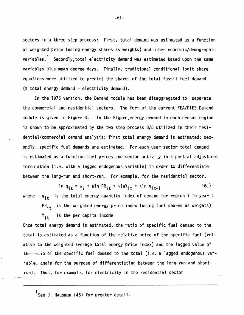
-61-

sectors in a three step process: first, total demand was estimated as a function

of weighted price (using energy shares as weights) and other economic/demographic

variables.l Secondly,total electricity demand was estimated based upon the same

variables plus mean degree days. Finally, traditional conditional logit share

equations were utilized to predict the shares of the total fossil fuel demand

(- total energy demand - electricity demand).

In the 1976 version, the Demand module has been disaggregated to separate

the commercial and residential sectors. The form of the current FEA/PIES Demand

module is given in Figure 3. In the Figure,energy demand in each census region

is shown to be approximated by the two step process B/J utilized in their resi-

dential/commercial demand analysis: first total energy demand is estimated; sec-

ondly, specific fuel demands are estimated. For each user sector total demand

is estimated as a function fuel prices and sector activity in a partial adjustment

formulation (i.e. with a lagged endogenous variable) in order to differentiate

between the long-run and short-run. For example, for the residential sector,

ln qit = ai + ln PRit + lnYit + ln qit-l 16a)

where qit is the total energy quantity index of demand for region i in year t

PRit is the weighted energy price index (using fuel shares as weights)

Yit is the per capita income

Once total energy demand is estimated, the ratio of specific fuel demand to the

total is estimated as a function of the relative price of the specific fuel (rel-

ative to the weighted average total energy price index) and the lagged value of

the ratio of the specific fuel demand to the total (i.e. a lagged endogenous var-

iable, again for the purpose of differentiating between the long-run and short-

run). Thus, for example, for electricity in the residential sector

1See J. Hausman (46) for greater detail.

-62-

In q it) =aei + e In e+ it-l 16b)it ~ei~ P- itqit-

where qe is the residential demand for electricity

Pe is the residential electricity price

e is the fuel specific subscript, here for electricity

qi and PRi are defined above

i and t are region and time subscripts

The individual fuels analyzed for the using sectors are indicated in Table 4.

Finally, the total price and quantity indices in each region are log-linear

value-weighted averages of regional prices or quantities; that is,

In qi = kiln qkik

In PRi : Vki In Pki 16c)k

where v P ki i q P qi

and Pki is the price of the kth fuel in region i

qki is the consumption of the kth fuel in region i

qi and PRi are defined above (the time subscript has been dropped)

Equation 16a) is estimated utilizing pooled time-series/cross-sectional

data (1960-1972) for the census regions). The price and activity variable co-

efficients are invariant with respect to time and region; however, regional spe-

cific intercepts are used. Likewise a regional specific first-order auto-correl-

ation transformation was used. Equation 16b) was estimated separately for each

of the nine census regions in similar fashion.

The.documentation for the FEA/PIES model is found in:-

* FEA, National Energy Outlook, 1976, FEA-N-TS/713, February 1976.

* FEA, Project Independence Blueprint, November 1974.

-63-

o Hausman, J., "Project Independence Report: An Appraisal of U.S. EnergyNeeds up to 1985," Bell Journal of Economics, Autumn 1975.

3) THE OAK RIDGE/HIRST et al. (OR/H) MODEL

The modelling efforts pursued by the group under Eric Hirst at Oak Ridge

National Laboratory have been limited in focus to the residential demand for

1energy. However while limiting their purview to residential demand alone and

by combining econometric,economic and engineering modelling tools, the Oak Ridge

group has developed a methodology rich in technological and policy detail. While

the model is complicated and perhaps confusing upon first reading, it merits

close scrutiny and understanding.

The OR/H model focuses upon four fuels (i = electricity, gas, oil and other)

for three housing types (m = single family, multi-family and mobile home) for

eight fuel end uses (k = space heating, water heating, refrigeration, food freezing,

cooking, air conditioning, lighting and other). Use of fuel i is then determined

in year t by housing type m for end use k as

Qt = ikm ikm ikm ik 17a)t t ' t t t

where HT is the stock of occupied housing units;

C is the market share of households with a particular type of fuel-burning

equipment;

TI is the thermal integrity of housing units (for space heating and air

conditioning only);

EU is the average energy use for the type of equipment (i.e. efficiency);

and

IOther efforts are being conducted directed at both industrial and commercialdemand.

-64-

U is a usage factor.

The Oak Ridge group utilize a combination of demographic models (to explain

and forecast housing stocks and flows), economic models (fuel demand and fuel

share analyses) and technology models (to examine the relationship between cap-

ital cost and efficiency/) to quantify the five components of equation 17a). The

housing model predicts the number of households by the age of household head each

year based upon population (for 7 age groups), per capita income and retirement

rates for each housing type.1 The model gives estimates of HTm ; hence it esti-

mates stocks and changes in the stock.

The fraction of households of type m that use fuel for end use k (C km) is

calculated by

i kmt

(l-Rk)Cikm HTt + Ckm NUkmt- HTt-1 + CNt t

HTmt17b)

where Rk

CNikmt

kmNut

CN, the market

is the equipment retirement rate for use k;

is the share of new equipment (NU) installed in t that uses

fuel i for end use k for housing type m; and

is the number of new units installed during t that provide end-use

k in housing type m.

share of new units, is calculated from an equation of the form

ikm

CNt Aikm + (Bijk EUNjkm jTIkm)In : ikm A Et UN TI

1 - CN jt~~~~~

3 + x (Cijk ·pEQjkm) + ik . Y

j=l t t17c)

1For greater detail see E. Hirst et al., "An Improved Engineering -- EconomicModel of Residential Energy Use," (49).

-65-

where X3 is fuel price for fuel j in year t;

EUNJkm is new equipment energy use (efficiency) for equipment using

j in end use k in housing type m;

TIjkm is average thermal integrity for housing type m using fuel jt

end use k;

PEQJkm is new equipment purchase price for equipment burning fuel j

end use k; and

Yt is per capita income.

fuel

in

in

A, B, C, and D are coeffecients estimated by utilizing parameter and elas-

ticity estimates from equations of the form:

Ink = a + zyiln Pi + Blln PCI + 2 In HDD + B31n COOL 17d)

n(1 Sk) = 0 + zyj n P + lzj In PEQj + 61 PCIi i j

+ 62 HDD + 63 CDD 17e)

where qk is the quantity consumed of fuel k/household.

Sk is the share of the equipment stock using fuel k for each end

use i.

Pi are the own and cross-prices of fuels.

PEQj are the equipment capital costs for alternative fuel-burning

equipment.

PCI is per capita income.

HDD is heating degree days.

COOL is mean July temperature.

CDD is cooling degree days.

Equation 17d) is similar to the single fuel equations found in Section C

while 17e) is similar to the logit share equation found in the discussions of

interfuel substitution in Sections D1 and D2 above. The OR/H logit equations,

-66-

however, at least include capital costs. However, for space heating, only an

oil equipment capital service price is used.l Additional economic/demographic

variables were tested in equations 17e). Dynamic (lagged endogenous variable)

and non-dynamic specifications were tested.

Based upon the parameter/elasticity estimates from equations 17d) and 17e)

the OR/H utilizes an "Elasticity Estimator" to quantify A, B, C and D in 17c).

The Elasticity Estimator is merely a set of semi-rigorous and/or ad hoc rela-

tionships developed to use the consumption elasticities (from 17d) and stock

share elasticities (from 17e) to quantify the new equipment share (A), price (B),

capital cost (C) and income (D) elasticities in 17c). While some of these re-

lationships are arbitrary, this approach does provide a strong link in 17c) be-

tween the technological changes in EUN, TI and/or PEQ, econcomic changes in fuel

prices and the fuel shares of new equipment purchases.

The EU terms (average annual equipment energy use) in 17a) are calculated as

EUN ikm ikm Nkm ikm Cikm HTm (1 - Rk)ikm t t t t-1 t-1 t- ) 17f)t cikm HTm

t H

where the terms of 17f) are all defined above. Likewise the thermal integrity

TI terms, which are applicable only to space heating and air conditioning equations,

are derived as in 17f). However TI can change through new housing units and ret-

rofitting, both of which the model deals with deterministically.

Finally U, the usage term is given by

1See Lin, Hirst and Cohn (60) for discussion of the logit estimates (equation17e). Estimation of equation 17d) is discussed in Cohn, Hirst and Jackson, "Econ-ometric Analyses of Household Fuel Demands" (28). The logit equations in 17e)improve upon the B/J equations because they are more generalized. See (43) and(45).

-67-

ik Eik + Fikn (X Ekm * TIkmIn U n (X EU ikt ) + G In Yt

ik ik+ Hikn Utl 17g)

where all variables are defined above and E, F, G and H are determined by the

Elasticity Estimator in a manner similar to that discussed above for equation

17c). 17g) makes the intensity of household use (capital stock utilization) a

function of incomes and operating costs of the equipment. Again, as found through-

out the model, energy use depends upon both economic and technological factors.

The documentation for the OR/H model and technology assessment is contained

in:the following:

* Eric Hirst, et al., "An Improved Engineering-Economic Model of ResidentialEnergy Use," Oak Ridge National Laboratory ORNL/CON-8 (April 1977).

* W.S. Chern, "Energy Demand and Interfuel Substitution in the CombinedResidential and Commercial Sector," Oak Ridge National Laboratory, ORNL/JM-5557 (September, 1976).

* Cohn, Steve, Eric Hirst and Jerry Jackson, "Econometric Analyses of House-hold Fuel Demands," Oak Ridge National Laboratory, ORNL/CON-7 (March, 1977).

* W. Lin, E. Hirst and S. Cohn, "Fuel Choices in the Household Sector," OakRidge National Laboratory," ORNL/CON-3 (October, 1976).

* J. Moyers, "The Room Air Conditioner as an Energy Consumer," Oak RidgeNational Laboratory, ORNL-NSF-EP-59 (1973).

· R. Hoskins and E. Hirst, "Energy and Cost Analysis of Residential WaterHeaters," Oak Ridge National Laboratory, ORNL-CON-10 (June 1977).

* R. Hoskins and E. Hirst, "Energy and Cost Analysis of Residential Refrig-erators," Oak Ridge National Laboratory, ORNL/CON-6 (January 1977).

4) ANDERSON MODEL

As discussed in Section C, Anderson has specified and estimated a number of

single fuel demand models. In addition, he has dealt with appliance stocks dif-

ferently than the usual conditional logit treatment. Anderson (6) focuses upon

the shares of new installations (new installments + conversions + replacements)

using a functional form approximating share s. by fi where*1

-68-

f 18a)zqj()jJ

where

zf i= 1 18b)i

and qi(' ) = ai. VCi d. 18c)

Pi is the price of energy i, vi is the appliance price of fuel equipment, y is

household income, and Z is a term including effects of all household-character-

istic variables. Approximating si (share of new installations using fuel i) by

fi ' ui' where ui is an error term, Anderson generates m - 1 equations of the form

Si i(u. a b. -b c ' m d ds qi ( ') ui ai b pv m iP. P v. V

Sm qm(') U a i m m

zi u.

Zm um 18d)m

where there exists m possible fuels to be used. Anderson uses log-linear forms

of 18d) and Zellners' seemingly unrelated equations estimating technique. An-

derson uses state cross-sectional data on home-heating for 1970 and 1960/1970 and

ultimately estimates equations of the form

n a + a. lnP. + a lnPm + a YPH + a In HSim i 1 m im l m

+ a3 SHU + a4 NuHu + aim WTEMP + u 18e)mm im lm

i = 1, ..., m - 1

where si, sm are the shares of home heating installations using fuels i and m

Pi' Pm are the fuel prices

-69-

YPH is annual income for household

HS is household size (persons/household)

SHU is the fraction of total housing that is single detached

housing units

NuHu is the fraction of total housing that is non-urban

WTEMP is mean December temperature

Similar equations with different independent variables are estimated for water

heating installations, cooking installations, washing and drying installations,

air conditioning, food freezing, dishwashing and television installations. The

resulting elasticity estimates are discussed in the summary to this section.

In equation 18d) Anderson appropriately dichotomizes the short-run and long-

run energy demand decisions by focusing upon the determinants of consumer demand

for changes in the stock of residential appliances. Equation 18d) is well-spec-

ified to analyze the determinants of that demand; it includes fuel operating

costs, income effects, demographic effects and the technical characteristics of

the appliances (summarized by appliance prices). Unfortunately, the estimated

equation does not include the appliance prices.

The single source for the model is

e K. Anderson, "Residential Energy Use: An Econometric Analysis," RandCorporation, R-1297-NSF (October 1973).

5) ERICKSON, SPANN AND CILIANO (ESC) MODEL

The ESC model is interested in both usage and substitution in energy demand

in the combined residential and commercial sector. Rather than using the trad-

itional log shares logit formulation however, ESC model fuel shares in new con-

struction as

sit = a + bxt 19a)

where sit is the share of new construction using fuel i in time t, and xt is the

-70-

vector of exogenous variables. In order to model actual demand, ESC model average

usage per consuming unit as

ut = a + b1 z 19b)

where zt are exogenous. Since

Sit = Sit-l + Sit - lit 19c)

where Sit is the market share of fuel i in time t, and

lit is the loss rate of market share for i and t.

Them residential and commercial demand Dit in time t for fuel i is given by

Dit = Sit * Nt * it 19d)

where Nt is the total number of households. Substituting, one has

Dit (Sit-l + a + bxt lit (a + b )N l9e)= t- zt)Nt 19e)

For the home heating share equations, ESC estimate equation 19a) for gas

and oil as follows:

In gas = a0 + alPg/P o + a2Pg/Pe + a3AC + a4u + a5y

+ a6Dl + a7D2 + a8D3 + a9D4 + alOS2

ln oil = b0 + blP/P + b2 Po/Pe + b3AC + b4u + b5Y

+ b6T1 + b7Dl + b8D2 + b9D3 + blOD4 + bllS2

where soil = The ratio of oil burners installed in new dwelling units to

total new construction

s Natural gas heating customers added via new construction divided

by total new construction

P0 = The average real price of fuel oil in dollars per barrel to the

residential market sector

P = The average real price of natural gas in dollars per cubic foot

to the residential market sector

-71-

U = An index of urbanization

Y = Real income per capita

S1 = The percent of new construction that is one or two-family

dwelling units

S2 = The percent of new construction that is four-family dwelling

units or less

T1 = Winter temperature

AC = The number of private one-family homes sold with air conditioning.

D1 to D4 = A set of dummy variables with Dl=l for Louisiana; D2=1 for Ok-

lahoma; D3=1 for Texas; and D4=1 for New Mexico.

Pe = The average real price of residential electricity

6) SUMMARY AND OVERVIEW

It will be recalled from Section C that there are three consumer decisions

that span the short-run and long-run (see p. 12). The single fuel models were

found to deal with these differences in one of three ways: 1) not at all; 2) im-

plicitly, through a partial adjustment formulation; or 3) explicitly, through multi-

equation capital stock/capital utilization analyses. The interfuel substitution

models likewise deal with the differences in several ways. B/J and FEA/PIES

utilize the partial adjustment/lagged endogenous variable formulation to differ-

entiate between the short-run and long-run. The OR/H model specifies annual fuel

demand in equation 17a) by explicitly analyzing the size of the housing stock,

the fuel shares of the stock and changes in the stock of several appliance types,

the thermal integrity of the housing stock, the efficiency of new and old appli-

ances and capital utilization. The equation incorporates past decisions built

into the appliance stock in addition to the consumer decisions (fuel shares)

built into the additions to the appliance stock (i.e., long-run decisions). The

-72-

OR/H model deals with short-run intensity of use decision explicitly through EU.

Thus OR/H deals explicitly with all three of the consumer decisions. However,

the model bases the parameters of analysis upon traditional static and dynamic

partial adjustment fuel share formulations 17e) and energy demand 17d) equations.

These traditional results are utilized for estimates of explicit short-run and

long-run elasticities; however, the estimation is ad hoc. Both Anderson and ESC

model shares in changes in the appliance stock, thereby dealing with decisions

1 and 2 explicitly.

A number of the corresponding long-run and short-run elasticity estimates

for these studies will be presented below in the summary comments. The comments

will follow the eight criteria of evaluation found in Section B.

i) Proper identification of the major market participants and the level of

analytic disaggregation required.

The B/J demand module focuses upon the aggregated commercial/residential

and industrial sectors, while ignoring transportation demand (unlike the FEA/PIES

model). B/J assesses demand for coal, oil, gas and electricity. Electric utility

demand is analyzed elsewhere in the B/J model. The exclusion of transportation

demand is a potential problem for several reasons. Its exclusion will understate

total demand for alternative fuels. Secondly, its exclusion will limit the policy

analysis use of the model by making it difficult to assess proposals for rapid

transit and electric autos. FEA/PIES focuses upon residential, commercial, in-

dustrial and transportation sectors separately. Furthermore the fuels examined

are disaggregated to a finer level of detail as indicated in Table 4. OR/H fo-

cuses upon residential demand for four fuels (gas, oil, electricity, other) for

eight fuel uses in three housing types. Anderson analyzes residential demand for

six fuels for a number of fuel uses. ESC focus upon residential and commercial

lGas, oil, electricity, bottled gas, kerosene, coal.

-73-

TABLE 4 : FUELS MODELED JOINTLY BY SECTOR

RESIDENTIAL SECTOR COMMERCIAL SECTOR INDUSTRIAL SECTOR

Electricity

Natural Gas

Distillate Oil

Kerosene

Liquid Gases

Electricity

Natural Gas

Distillate Oil

Residual Oil

Electricity

Natural Gas

Distillate Oil

Residual Oil

Kerosene

Liquid Gases

Coal

-74-

home heating demand.

The lack of disaggregation of the two sectors in the B/J model is not a

serious difficulty given the analytic aims of the authors. B/J appear to have

been most interested in analyzing fuel supply and the financial/regulatory en-

vironment of the electric utility industry. As a result, they looked to close

the demand side of the model with an aggregate energy demand module that provided

little in the way of disaggregated policy analysis. However, greater disaggre-

gation would be necessary if any short-run conservation policies and long-run

demand for new technologies were to be analyzed with the demand module. For ex-

ample appliance efficiency taxes, appliance efficiency standards, heating ther-

mostat controls and the technical characteristics of new technologies are use-

specific for the residential, commercial, and industrial demands. Incorporation

of such technological and policy variables would require use-specific analyses.

Such use-specific analysis would also permit differentiation of use-specific price

elasticities. For example, in Figure 4A, aggregate B/J commercial/residential

short-run price elasticities are presented while Figure 4B presents B/J elasticity

estimates for four specific residential uses. As is seen in the two figures,

disaggregation provides widely different estimates of the relevant elasticities.

The FEA/PIES model provides greater disaggregation by breaking out the

residential and commercial sectors and by further disaggregating the fuels used

by the residential, commercial and industrial sectors (see Table 3). Thus FEA/

PIES provides greater refinement for assessing policy proposals for the residen-

tial and commercial sectors separately. It furthermore permits refined assessment

of more fuel-specific policies, such as BTU taxes on alternative fuels. The OR/H

focuses upon residential demand and provides a high degree of disaggregation by

fuel, fuel use and housing type. Furthermore,it is the only model that deals

explicitly with such engineering/policy considerations as the thermal integrity

-75-

FIGURE 4A : AGGREGATE RESIDENTIAL AND COMMERCIAL SECTOR

SHORT-RUN SHARE ELASTICITIES

Pe Po Pg

Se -0.800 0.284 0.514

SO 0.414 -0.929 0.514

Sg 0.414 0.284 -0.698g

Source: Baughman and Joskow (13)

-76-

FIGURE 4B : DISAGGREGATED SHORT-RUN FUEL SHARE ELASTICITIES FOR

PARTICULAR RESIDENTIAL USES

HOUSE HEATING

Pe

Electricity

Gas

Oil

Pg

-2.08

.23

.23

2.12

-1.48

2.12

P0

3.30

3.30

-7.21

WATER HEATING

P P Pe g o

Electricity

Gas

Oil

COOKING FUEL

P Pe g

Electricity

Gas

CLOTHES DRYERS

P PP

Electricity

Gas

- .58

2.05

g

.53

-1.99

Source: Baughman and Joskow (9)

e

-77-

(TI) of the residential structures, the average energy use (EU) for types of

equipment (i.e. efficiency), a usage factor (U) for the equipment (i.e. short-

run demand given capital in place) and capital cost characteristics of alter-

native fuel-burning equipment [see equation 17a) and 17e)]. Thus the OR/H model

provides the richest specifications and disaggregation for policy purposes; ap-

pliance efficiency taxes and standards, heating thermostat controls and the cap-

ital cost and technological characteristics of new technologies could be intro-

duced into the model and the effects upon residential energy demand assessed.

The Anderson demand analysis is disaggregated by eight fuels for residential

demand; however the independent variables available for policy analysis are only

operating costs. Hence as with B/J there is little room for more extensive policy

analysis. The ESC model examines only gas and oil explicitly (electricity share

is a residual) and there exist no real policy variables except operating costs.

Of the models reviewed, only B/J and FEA/PIES assess industrial demand.

For this sector, greater disaggregation along two-digit SIC's for process and

comfort use would be extremely useful. Such disaggregation would permit the an-

alysis to be technology/process specific and hopefully permit the introduction

of capital stock characteristics, particularly fuel-burning equipment character-

istics. However, the data problems are significant and it is not clear that such

disaggregation is possible at the moment without an onerous data gathering effort.

ii) Proper identification and incorporation into variables in the model of

policy issues and technological consideration for the major market participants.

As mentioned above, the level of aggregation in the B/J and FEA/PIES demand

modules precludes the efficient incorporation of several use-specific technol-

ogical characterizations and policy variables. This is a difficulty for properly

assessing the three consumer-decisions spanning the short-run and the long-run

and for assessing new technologies. However, in spite of the aggregation, other

-78-

policy variables could have been incorporated including, for example, average

appliance efficiency, average fuel efficiency and capital costs of alternative

fuel-burning equipment. The only policy variable available to the analyst in

the B/J, FEA/PIES, and ESC demand modules is the operating cost of alternative

fuels -- an extremely limited policy variable. No technological characteristics

of alternative fuels and their relevant equipment are included. The availability

of a single price-based policy variable ignores the use-specific policy options

mentioned above: appliance efficiency taxes and standards, thermostat controls,

speed limits. Furthermore, while B/J and FEA/PIES utilize a partial adjustment

formulation in order to differentiate between the short-run and long-run, this

formulation still ignores the important differences between short-run and long-

run policy options: in the short-run, (fixed stock of capital and fuel-burning

equipment) conservation and capital utilization policies are relevant while in

the long-run, (variable stock of capital and fuel-burning equipment) policies

aimed at new technologies and improved appliance efficiency are important.

The OR/H model does the best job of providing a framework for dealing with

the technological and cost characteristics of old and new technologies and spe-

cific policy proposals within a well specified dichotomization of the short-run

and long-run behavioral differences.

As a specific example of policy analysis, B/J utilize the model to assess

several electric utility policy proposals in Joskow and Baughman (58). The policy

possibilities include higher air pollution restrictions, peak load pricing, de-

creased nuclear plant lead times, a nuclear moratorium, higher costs of capital,

and higher costs of uranium ore and enrichment. All of the policy proposals have

important and far-reaching effects. However, the simulation of several proposals,

particularly peak load pricing policies, requires a level of detailed sophisti-

cation lacking in the average electricity price generated in the Regulatory-Fi-

-79-

nancial module of the B/J model and exogenously applied to the demand module.

One example of a more detailed analysis is the multi-tariff work done by Taylor,

Blattenberger, Verleger/DRI (reviewed in Section B).

iii) Proper degree of geographical disaggregation.

All five models reviewed utilize either cross-sectional or a pooled time-

series of cross-sections where the cross-sections are by states. Such state de-

tail in the data provides the ability to test and simulate regional homogeneity.

Hence the models possess the data and techniques to be quite regionally disaggre-

gated. Furthermore, the B/J and FEA/PIES models do simulate on a regional basis.

(for Census regions). Such regional disaggregation is appropriate for most policy

analysis.

iv) Utilization of the appropriate behavioral models and underlying be-

havioral assumptions.

As mentioned in the preceding paragraphs, there exists important behavioral

and policy differences for short-run and long-run energy demands which require

more refined behavioral specifications, technological characterizations and policy

variables than fuel prices alone. The important differences between the short-

run and the long-run argue for explicit multi-equation analysis of the separate

phenomena. The B/J and FEA/PIES demand modules deal with the difference by

utilizing a standard single equation partial adjustment formulation. Such a

partial adjustment formulation is an acceptable first-cut technique; however,

it has difficulties. In addition to the lack of specificity of the differences

between the long-run and short-run (mentioned under criteria ii) the partial ad-

justment formulation's use of a lagged endogenous variable presents econometric

difficulties. In the presence of a serial correlation, potential parameter

estimate inconsistencies arise. Furthermore, the lagged adjustment parameter

estimate is extremely sensitive to sample period and stochastic specification.

-80-

Since we are particularly interested in the difference between short-run and long-

run consumer-reactions and since the parameter estimated for the lagged endogenous

variable is crucial in estimating the difference between short-run and long-run

responses, these estimated differences will also be quite sensitive to the sample

and the assumed stochastic specification.

A second problem involves the behavioral assumptions underlying the B/J and

FEA/PIES demand modules. Total national demand (for the B/J industrial sector)

or state energy demand (for the B/J and FEA/PIES commercial and residential sec-

tors) are estimated, and these totals are disaggregated into location and par-

ticular fuels assuming cost-minimizing behavior on the part of the relevant par-

ticipant. Such sequential "trickle-down" decision making implies that consumers

decide on the total energy demand independent of their location and their capital

stock and fuel-burning equipment. Once these consumers decide on total energy

needs, they decide on location (for industry in B/J) and type f fuel to be

utilized (for industrial, commercial and residential in FEA/PiIES and residential/

commercial in B/J).

Such assumed decision-making may generate believable results at the aggre-

gate residential/commercial sector level. However, at the disaggregated use-

specific level such trickle-down decision making can lead to contradictions. The

reason is that consumers will cost minimize in choosing alternative locations and/

or fuels in the long-run when changes in the stock of capital and fuel-burning

equipment are possible. In the short-run, relocation and interfuel substitution

are nearly impossible. The contradictions can arise in B/J when the share equa-

tions are applied to total energy demand and the predicted fuel shares imply ap-

liance stock changes that are larger than possible.

The direction of causation in these models seems to be reversed. Rather

than modelling the aggregate and breaking out the components, it seems that

-81-

explicit micro modelling of the short-run and long-run demands for alternative

fuels and equipment should be performed and then aggregated to the totals.

The OR/H, Anderson and ESC models improve upon this treatment. They do not

utilize a partial adjustment formulation to differentiate the long-run and short-

run. Rather, all three models deal with the fuel shares in the changes in the

appliance stock, where consumer decisions are actually exerted. The OR/H an-

alyzes demand at the micro level (for fuel, fuel use and residential structure)

and aggregates rather than assuming a "trickle down" decision process. It also

provides the best example of explicit multi-equation analysis of short-run and

long-run issues including: short-run demand for fuels given appliance stocks;

and long-run demand for old and new technologies in the additions to the appliance

stock, based upon operating costs, capital costs and appliance effiencies.

The utilization of conditional logit (by B/J, FEA/PIES and OR/H) or other

share analysis techniques (Anderson, ESC) presents varying problems. The con-

ditional logit formulation utilized by B/J in the fuel split equations for both

sectors is inappropriate for the following reasons: the imposition of constant

cross-elasticities [see Baughman and Joskow ((9), (12), (13)), Domencith:andlIMc-

Fadden (32), Hartman (43), Hartman and Hollyer (45)]; implied misspecification

[see Hartman (43) and Hartman and Hllyer (45)]; excluded variables; and the res-

trictive underlying model of individual choices [see Hartman (43) and Hartman and

Hollyer (45)]. The 1974 FEA/PIES model imposed constant cross-elasticities [see

Hausman (46)] and suffered from the same problems listed above. The 1976 FEA/

PIES model avoids some of these difficulties but forces cross-elasticities to be

zero (see equation 16b) while also suffering from excluded variables (cross-

prices and capital costs to name.a few -see Hartman and Hollyer (45)) and the

restrictive model of individual choice [see Hartman and Hollyer (45)).

To indicate the effects of some oflthe difficulties Figure 5 compares elas-

-82-

FIGURE 5 : COMPARISON WITH ALTERNATIVE ANALYSES : PRICE ELASTICITIES

OF FUEL SHARES, RESIDENTIAL SPACE HEATING

UNCONSTRAINED CROSS ELASTICITIES

Log-Loga) Lin, Hirst and Cohn

Semi-Loga) Lin, Hirst and Cohn

Pe Pg Po Pe Pg Po

Space Heating

Electricity

Gas

Oil

-2.63 0.44

0.39 -1.57

1.37

0.03

0.03 3.51 -1.09

-3.19 0.38 1.09

0.57 -1.33 0.03

-0.18 2.95 -1.01

CONSTRAINED CROSS ELASTICITIES

b) Anderson

Pe Pg Po

c) Baughman & Joskow

Pe Pg Po

Space Heating

Electricity

Gas

Oil

-2.04 2.21 0.55

0.17 -1.80 0.55

0.17 2.21 -1.58

-2.08 2.12 3.30

0.23 -1.48 3.30

0.23 2.12 -7.21

Sources

a) Lin, Hirst and Cohn (60)

b) Anderson (4)

c) B/J (9)

-83-

ticity estimates of B/J with those of Anderson (4) and OR/H [Lin, Hirst and Cohn

(60)]. The conditional logit-formulation of B/J and Anderson methodology impose

constant cross-elasticities. The Lin, Hirst and Cohn analyses utilize a more

general logit formulation which avoids the misspecification [Hartman (43)] and

permits the estimation of differential cross-elasticities,as are documented in

Figure 5.

Furthermore, the fuel split equations for B/J and FEA/PIES (34 and 35), as

stated above, include only fuel costs; hence they ignore capital costs, non-

price characteristics of alternative fuels, personal characteristics of the fuel-

choosing population and new technologies. ESC and Anderson ignore capital costs

but include personal and demographic factors. Figure 6 indicates fuel share

elasticities with capital costs included. Some elasticity estimates are the

wrong sign; some of these incorrect signs result from coefficients not signifi-

cantly different from zero. The point to be made is the inclusion of excluded

variables does change price elasticity estimates considerably (compare Figure 5

with Figure 6).

For comparability of the analyses, the elasticities in Figures 4-6 have been

based upon a logit specification without a partial adjustment formulation; that

is logit share equations are applied to the stock of appliances. If a partial

adjustment formulation were built into all of them, the results should differ in

the same fashion as indicated in Figures 4-6. However, the underlying model of

consumer choice is most valid when applied to changes in the stock of appliances.

Figure 7 presents for comparison, fuel share elasticities for changes in the

housing/appliance stock. As Figure 7 indicates, the elasticity estimates again

differ considerably from those in Figures 4-6. OR/H, Anderson and ESC do an-

alyze changes in the equipment stock.

In the face of such alternate estimates one must seek a model that best ap-

-84-

FIGURE 6 : RESIDENTIAL HOME HEATING FUEL SHARE ELASTICITIES

WITH CAPITAL COSTS INCLUDED

ShareElectricity

-3.86

2.34

0.278

-10.4

10.3

-1.82

0.865E-01

0.954

-0.558E-01

ShareOil

-1.47

-0.521

1.69

4.45

-34.4

31.4

-1.66

-0.261

0.578

ShareGas.

1.31

0.136

-1.13

-2.01

21.7

-20.5

1.08

0.867E-0Q1

-0.375

Source:

Hartman and Hollyer (45)

Pe

Po

Pg

CAPe

CAPo

CAPg

AV

PCI

TEMP

-85-

FIGURE 7 : SHARE ELASTICITIES FOR CHANGES IN THE HOUSING STOCK,

HOME HEATING

Pe Pg Po PCI

-1.567 1.286

.730 - .611

2.491 4.037

.245 -1.203(0)*

- .437(0)* .568(0)*

-10.829 -1.654(0)*

*Elasticity value if parameters not significantly different from zero

are set to zero.

Source: Hartman and Hollyer (45)

Se

SgSo

-86-

proximates consumer choice without imposing misspecification or severe restrictions

upon the behavioral estimates.

While the preceding discussion was directed primarily at residential and

commercial demand modelling, there exist some difficulties in the two models that

address industrial demand modelling (B/J and FEA/PIES). Since the FEA/PIES model

treats industrial demand the same as commercial and residential demand, the same

problems exist as discussed above. Furthermore, both B/J and FEA/PIES ignore

more detailed production analysis. Admittedly, at the time the B/J and FEA/PIES

(34) analyses were performed, some of the more sophisticated production/cost

duality approaches had not been popularized [Econometrical International (33)].

However, there existed enough of a literature to more credibly approach the

problem. The prices of all other factors of production are ignored in Baughman

and Zerhoot (11) and in FEA/PIES. Capital service prices are at least added in

Joskow and Baughman (58). However, there remain serious inadequacies in the in-

dustrial demand modelling. The B/J and FEA/PIES models have not adequately dealt

with the details of industrial production technology, even at an aggregate level,

nor its formal relationship to derived demand.

Furthermore, while FEA/PIES does differentiate between long-run and short-

run demand through a partial adjustment formulation, the national industrial en-

ergy demand analysis of B/J does not. Baughman and Zerhoot (11) claim that at-

tempts to build in lagged responses were unsuccessful. It is claimed an Almon

lag specification was not attempted because it would only worsen multi-collin-

earity compared to unconstrained lag estimation. That is, unfortunately, not

true; the use of the Almon lag should lessen multi-collinearity problems. Fur-

thermore, the Koyck lag specification implies an adjustment time of two years:

that is too short to be believable. As a result, Baughman and Zerhoot (11) and

Joskow and Baughman (58) do not use a lag specification, implying price response

-87-

is; immediate (i.e. within a year) for aggregate energy demand. That is not a

particularly useful or believable assumption to impose.

v) Proper integration of the demand module into an overall energy and/or

macroeconomic model.

All five models require the specification of exogenous variables in order

to do policy simulation. However, only the B/J and FEA/PIES are general equil-

ibrium in the sense that they deal with supply and demand and market clearing

for all sources and uses of the fuels analyzed. The FEA/PIES model utilizes a

linear programming integrating model which recursively converges to a market

equilibrium solution for all supplies and demands. This provision is a major

innovation and an extremely desirable feature of the model. Its desirability

can be assessed by comparing this procedure with the B/J model. The B/J de-

mand module is not solved simultaneously with the full model. Thus, while en-

dogenous to fuel supply sectors, alternative fuel prices are exogenous to the

demand module. As a result, non-marginal shifts in demand for alternative fuels

are not permitted to "play back" upon supply. In essence, supply is assumed in-

finitely elastic at the exogenous price.

The failure to deal with such simultaneities for non-marginal demand shifts

could generate serious errors in the analysis of the impacts of particular policies.

For example, policies aimed at large regional (say New England) shifts of demand

to coal must take account of the bottlenecks caused by the transportation (rail-

road) infrastructure. Non-marginal demand shifts to coal could push demand be-

yond the short-run transportation bottleneck, thereby making the short-run supply

price infinite. Likewise, non-marginal shifts in gas demand in New England have

historically led to imported LNG from Algeria at a supply price well above domestic

gas. The assumption of infinitely elastic supply at a constant price ignores

these realities and distorts projected fuel demands as a result.

-88-

vi) Utilization of proper data and statistical/econometric techniques

The econometric techniques utilized by the five interfuel substitution models

are more or less state of the art. Two stage least squares (2SLS) is utilized in

the presence of serial correlation and a lagged endogenous variable; however, the

models do not document the instruments used. However, it must be stated that the

simulation results are, in general, extremely sensitive to model specification,

variable definition and sample period of estimation. Figures 8A-8D demonstrates

simulation differences between the B/J and FEA (34) model for fuel price scenarios

outlined in Figure 8A. Figures 8C and 8D indicate several wide divergences and

the reasons.

vii) Provision of good documentation for the use of energy demand modelling.

All five models score well under this criteria.

viii) Provision for relatively easy accessibility and extensibility of the

modelling effort.

All five models are accessible. However B/J,FEA/PIES and OR/H are quite

large: hence while accessible, the extensibility depends upon how complicated

the desired changes are.

-89-

FIGURE 8A: REAL PRICES (1974 DOLLARS) USED FOR B/J AND

FEA INDUSTRIAL SIMULATIONS

CASE I - F.E.A. $11 per barrel

Oil Price Natural Gas Coal Price ElectricityPrice Price

($/Bbl) (tMCF) ($/ton) (t/Kwhr)

1975 6.70 64.2 10.44 2.39

1980 10.34 64.2 10.44 2.46

1985 10.86 64.2 10.44 2.27

CASE II - F.E.A. $7 per barrel

1975 5.50 64.2 10.44 2.39

1980 7.00 64.2 10.44 2.46

1985 7.00 64.2 10.44 2.27

CASE III - No O.P.E.C. (2% per year real increase)

1975 4.16 62.4 7.80 1.96

1980 4.59 68.9 8.62 1.99

1985 5.07 76.1 9.52 1.87

Oil is average price at the wellhead

Gas is average price at the wellhead

Coal is average price at the minemouth

Electricity is average price per kilowatt-hour consumed

-90-

FIGURE 8B: U.S. SIMULATION RESULTS (B/J AND FEA MODELS)

QUADRILLIONS OF BTU's INDUSTRIAL SECTOR

1972 Actual

Actual

1975 CASE I

(FEA Model)

(B/J Model)

:(B/J Model)

CASE II (B/J Model)

CASE III (B/J Model)

1980 CASE

CASE

CASE

CASE

CASE

1985 CASE

CASE

CASE

CASE

CASE

I

I

II

II

III

I

I

II

II

III

(FEA

(B/J

(FEA

(B/J

(B/J

(FEA

(B/J

(FEA

(B/J

(B/J

Model)

Model)

Model)

Model)

Model)

Model)

Model)

Model)

Model)

Model)

TOTAL

23.0

19.7

18.6

18.7

19.1

26.0

20.0

27.4

20.3

20.4

28.7

22.3

30.6

22.6

22.2

GAS

10.6

11.8

11.8

11.7

11.6

10.1

13.0

9.8

12.7

11.4

10.5

14.1

9.7

13.7

11.3

OIL

5.7

2.1

2.0

2.1

2.3

6.6

1.4

7.8

2.0

2.9

7.4

1.1

9.3

2.0

3.4

ELECTRICITY

2.5

2.2

2.5

2.5

2.5

3.3

3.4

3.7

3.3

3.4

4.1

4.4

4.6

4.2

4.5

CASE III = No O.P.E.C.

COAL

4.3

3.5

2.3

2.3

2.6

5.9

2.3

6.0

2.3

2.7

6.7

2.7

6.9

2.6

3.1, . _l ---

CASE I = $11/Bbl. CASE II = $7/Bbl.

-91-

FIGURE 8C : MAJOR DIVERGENCES BETWEEN B/J AND F.E.A. SIMULATIONS

1. B/J projected gas consumption increases by about 20%

from 1972 to 1985 for the price scenarios used, but

the F.E.A. gas consumption projections decrease for the

same price scenarios.

2. B/J projected oil consumption decreases by 1985 to about

50% of 1972 for $11 per barrel oil and remains essentially

constant for $7 per barrel oil, but the F.E.A. projects a

30% increase for $11 per barrel and a 60% increase for $7

per barrel oil. (The major reason for this is the B/J

exclusion of feedstocks.)

3. B/J projected coal consumption decreased by about 25% by 1985

for the price scenarios used, while the F.E.A. projects a 50-60%

increase in coal consumption by 1985. In addition, as the oil

consumption increases, while B/J model demonstrates the opposite

trend in behavior.

4. Where, by 1985, the F.E.A. model results in 25% and 33% increases

in total industrial energy consumption for the $11 and $7 per barrel

cases, respectively, the B/J model results in 13% and 15% increases.

(Again, part of the difference us due to feedstocks.)

-92-

FIGURE 8D : REASONS FOR GAS AND COAL DIVERGENCIES

1. The F.E.A. model has an own-price elasticity for natural gas

of -1.5 vs. an estimated value of -0.8 in B/J model.

2. The F.E.A. model has an own-price elasticity for coal of

-0.59 vs. an estimated value of -1.1 in the B/J model.

3. The F.E.A. model exhibits a negative cross-elasticity between

coal consumption and oil prices.

Source for Figures 8A - 8D : Baughman and Zerhoot (11)

-93-

E) SUMMARY AND STATEMENT OF FURTHER RESEARCH

It will be recalled that the intent of this model review has been to assess

the ability of each of the models firstly to specify and analyze the behavioral

characteristics of long-run and short-run demand and secondly to provide a frame-

work for examining the competitiveness of new technologies, particularly solar

photovoltaics. The behavioral components of short-run and long-run demand were

found to include three decisions:

* The consumer decision of whether to buy a fuel-burning consumer durable,

capable of providing a particular consumer service (e.g. cooking, heating,

lighting, air conditioning, etc.).

* The consumer decision about the characteristics fo the equipment purchased,

technical characteristics and whether the equipment embodies a new tech-

nology.

e Given consumer equipment the consumer decision about the frequency and

intensity of use.

All of the models treated these components of demand and new technologies with

varying degrees of success. However even the best of the models require some

improvement.

This Section first summarizes the model review. Based upon the summary and

the actual review, the most important deficiencies in the current generation of

energy demand models are identified. Sections El and E2 propose a model of res-

idential energy demand that attempts to incorporate the strengths and avoid or

improve upon the weaknesses in the models. Finally Section E3 presents an over-

view of ongoing efforts to accomplish the proposed model reformulation.

SUMMARY

Sections C and D reviewed but a portion of the energy demand models that

have appeared over the past ten years. The discussion in those sections has

-94-

principally focused upon econometric or econometric/process/engineering models.

The modelling efforts were divided into two groups: 1) models dealing with

overall energy demand and interfuel substitution and 2) models dealing with the

demand for a single fuel. The models reviewed in each category are repeated in

Figure 9. The lists are by no means exhaustive; they hopefully span model space,

forming a useful basis for suggestions for further research.

The B/J and FEA/PIES models represent generally the state of the art in

overall energy demand modelling. By state of the art, I mean that they have,

for the most part, utilized current theoretical and empirical techniques to model

the demand for all energy forms on the part of the residential, commercial and

industrial sectors, stressing interfuel substitution and explicitly approximating

the differences between the long-run and short-run with a partial adjustment

formulation. However while being state of the art these models exhibit a number

of weaknesses. The strengths and weaknesses have been discussed in Section D.

An apparent reason for the methodological shortcomings in the FEA and B/J

models is that in attempting to deal with the overall energy system, they have

sacrificed important details. The models lack, for example, the richness of

policy variables the extent of technological specificity and the multi-equation

behavioral specification found in the interfuel substitution model of OR/H.

However the OR/H modelling efforts deal only with the residential sector. Fur-

thermore, the OR/H effort still relies on traditional logit analyses of consumer

choice; as a result, while providing the best tool for residential energy de-

mand analysis available, greater effort on modelling consumer choice and new

technologies is required.

The B/J and FEA/PIES models also have less detail than many of the single

fuel demand models, for example the Anderson (3) and Halvorsen (41) models. How-

ever, these works deal only with equilibrium electricity demand, ignoring inter-

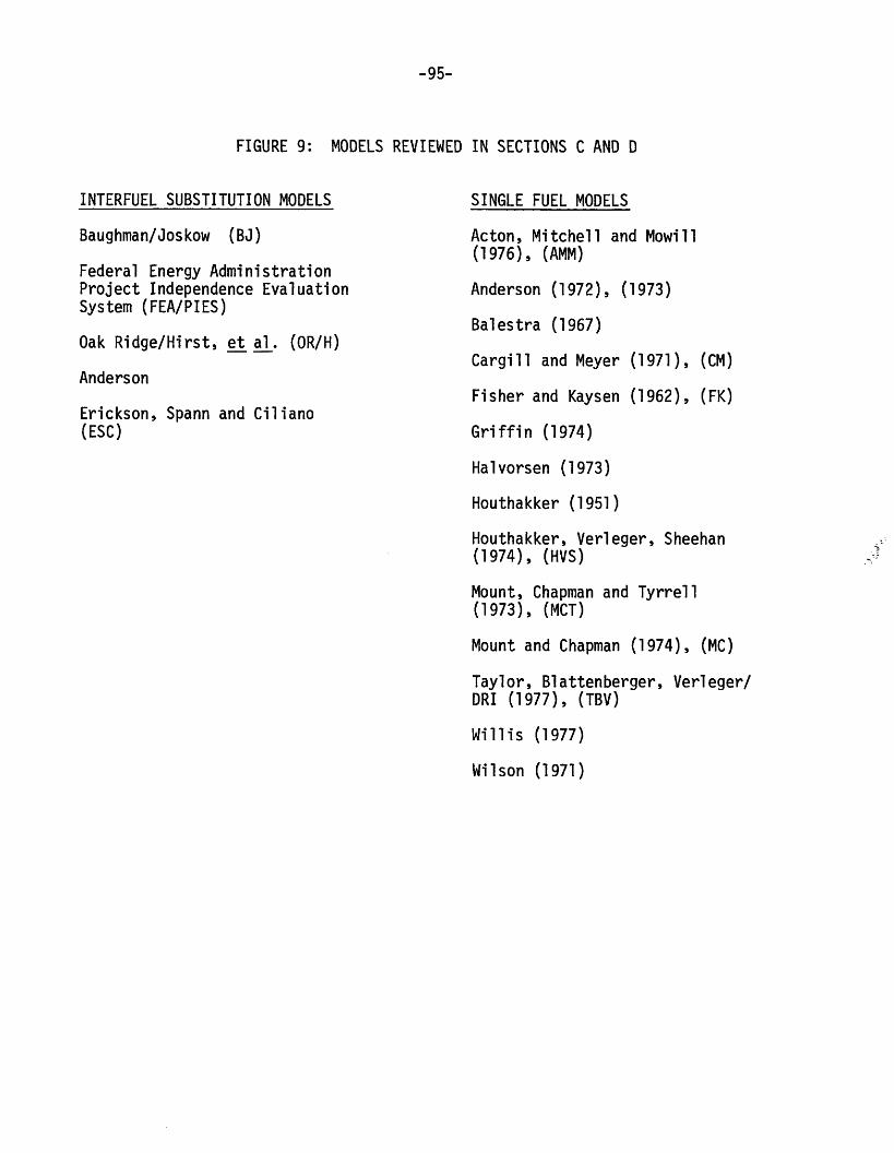
-95-

FIGURE 9: MODELS REVIEWED IN SECTIONS C AND D

INTERFUEL SUBSTITUTION MODELS

Baughman/Joskow (BJ)

Federal Energy AdministrationProject Independence EvaluationSystem (FEA/PIES)

Oak Ridge/Hirst, et al. (OR/H)

Anderson

Erickson, Spann and Ciliano(ESC)

SINGLE FUEL MODELS

Acton, Mitchell and Mowill(1976), (AMM)

Anderson (1972), (1973)

Balestra (1967)

Cargill and Meyer (1971), (CM)

Fisher and Kaysen (1962), (FK)

Griffin (1974)

Halvorsen (1973)

Houthakker (1951)

Houthakker, Verleger, Sheehan(1974), (HVS)

Mount, Chapman and Tyrrell(1973), (MCT)

Mount and Chapman (1974), (MC)

Taylor, Blattenberger, Verleger/DRI (1977), (TBV)

Willis (1977)

Wilson (1971)

-96-

fuel substitution and the differences between the long-run and short-run. The

partial adjustment residential models of Mount, Chapman and Tyrrell [MCT, (68)]

and Houthakker, Verleger, Sheehan [HVS, (56)] also focus upon electricity demand

alone.l While these single fuel models provide more detail than the B/J and FEA/

PIES models for electricity demand, they ignore gas and oil demands. These sin-

gle fuel models provide greater disaggregation than B/J and FEA/PIES by analyzing

the residential sector alone. Furthermore, Mount, Chapman and Tyrrell [MCT, (68)]

also explicitly disaggregate and analyze the commercial sector demand for elec-

tricity along similar analytic lines applied to the residential sector. The MCT

(68) industrial model and particularly the Anderson industrial model show greater

analytic sophistication than B/J and FEA/PIES; however, these efforts again con-

centrate only upon electricity demand. The Taylor, Blattenberger, Verleger/DRI

(TBV); Acton, Mitchell and Mowill (AMM); and Fisher and Kaysen (FK) analyses of

the residential demand for electricity introduce the short-run constraints em-

bodied in the stock of residential energy-consuming equipment. TBV and AMM

utilize a theoretically more sound multi-part tariff formulation rather than the

usual typical electric bill or average electricity price.

While the B/J and FEA/PIES efforts reflect state of the art in overall energy

models and in spite of the fact that single fuel demand analyses provide greater

analytic refinement, extended efforts are still required to properly differentiate

and delineate the short-run and long-run characteristics of demand and to properly

evaluate the potential of new technologies. The entire generation of energy de-

mand models that B/J, FEA/PIES and other efforts reflect have reached a stage of

forced obsolescence. New work done on choice modelling (generalized logit [Hartman

(43)] and covariance probit [Hausman and Wise (47)], production/cost duality [Econo-

1Many of these models are compared in greater detail in Charles RiverAssociates (25).

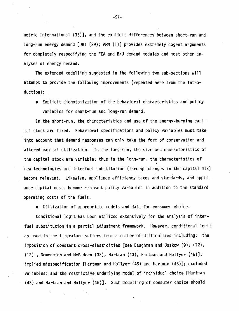
-97-

metric International (33)], and the explicit differences between short-run and

long-run energy demand [DRI (29); AMM (1)] provides extremely cogent arguments

for completely respecifying the FEA and B/J demand modules and most other an-

alyses of energy demand.

The extended modelling suggested in the following two sub-sections will

attempt to provide the following improvements (repeated here from the Intro-

duction):

· Explicit dichotomization of the behavioral characteristics and policy

variables for short-run and long-run demand.

In the short-run, the characteristics and use of the energy-burning capi-

tal stock are fixed. Behavioral specifications and policy variables must take

into account that demand responses can only take the form of conservation and

altered capital utilization. In the long-run, the size and characteristics of

the capital stock are variable; thus in the long-run, the characteristics of

new technologies and interfuel substitution (through changes in the capital mix)

become relevant. Likewise, appliance efficiency taxes and standards, and appli-

ance capital costs become relevant policy variables in addition to the standard

operating costs of the fuels.

* Utilization of appropriate models and data for consumer choice.

Conditional logit has been utilized extensively for the analysis of inter-

fuel substitution in a partial adjustment framework. However, conditional logit

as used in the literature suffers from a number of difficulties including: the

imposition of constant cross-elasticities [see Baughman and Joskow (9); (12),

(13) , Domencich and McFadden (32), Hartman (43), Hartman and Hollyer (45)];

implied misspecification [Hartman and Hollyer (45) and Hartman (43)]; excluded

variables; and the restrictive underlying model of individual choice [Hartman

(43) and Hartman and Hollyer (45)]. Such modelling of consumer choice should

-98-

utilize generalized logit formulations [Hartman (43)] orcovariance probit form-

ulations [Hausman and Wise (47)]. Furthermore the choice methodologies should be

applied to changes in the appliance stock rather than the actual stock [see Hart-

man and Hollyer (45)].

* Appropriate treatment of new technologies.

While generalized logit and covariance probit avoid some of the difficulties

inherent in conditional logit, the treatment of new technologies is not trivial

for either new alternative and careful formulation is required.

The modelling research proposed here is currently being pursued under con-

tract to the Department of Energy.

1) OVERVIEW OF THE PROPOSED MODEL REFORMULATION

Figure 10 provides an overview of the proposed model. In 10A, short-run

demand (di) is explicitly modeled for the fuels (i) = electricity (e), gas (g),

oil (o) and coal (c). Short-run demand for fuel i (di) is made a function of

own-price and cross-prices of fuels (Pj); the efficiencies of the stock of fuel-

burning equipment (EFFj); the size of the fixed stocks of the fuel-burning equip-

ment (Kj); income (y); climatic variables (TEMP, including heating and cooling

degree days); demographic factors (DEM, including a regional dummy and percentage

of families in single family homes); and other exogenous variables (Xil). For

data reasons, the short-run is assumed to be a year; hence, the fuel-burning

equipment stocks (Kj) and their characteristics (EFFj) are considered fixed.

This is not a particularly severe assumption for the more important uses of fuels.

The short-run formulation will be discussed more fully below, as well as the

specific fuel uses to be analyzed.

This proposed treatment of short-run demand for individual fuels is, in gen-

eral, similar to that of FK, AMM, TBV and Wills in that appliance stocks are taken

as given and demand is a capacity utilization issue. These single fuel models

99-

FIGURE 10: OVERVIEW OF RESIDENTIAL DEMAND MODEL

A) SHORT-RUN DEMAND:

d.i = Fi(P j, EFFj, Kj, y, TEMP, DEM, Xil ) ; i j = e, g, o, c

B) LONG-RUN DEMAND:

= Gi (Pi', EFFi , CAPi , Xi2) i = e, g, o,.c

* Kit = AKt Si (must predict AK)

Kit+l = Kit( - i) + aKit

Share equations utilizing Logit or Probit

C) TREATMENT OF NEW TECHNOLOGIES--DETERMINATION OF CAP., EFFi:

* Exogenously; then into share equations

* Endogenously

a) Specify discount rate and efficiency/capital cost

tradeoff, yielding EFFi and CAPi

b) Capital efficiency supply and demand model:

D: CAP i = Di (EFF i, EFFj, Pi, Pj, y, X3)

S: CAP i = Si (EFFj)

S.1

-1'00-

are the best of the reviewed group in meeting model evaluation criteria ii) and

iv): proper identification and incorporation into variables in the model of policy

issues and technological considerations for the major market participants; and

utilization of the appropriate behavioral models and underlying behavioral as-

sumptions. The demand formulation here is intended to incorporate the insights

and variables of those analyses and extended the effort to include characterization

of the effeciency of the appliance stock (EFFj). Much effort has been expended

for six fuel uses, as discussed in Section E2.

Figure 10B indicates the form of the long-run analysis. In the long-run,

the stock and characteristics of the residential fuel-burning equipment will be

variable. The first long-run equation states that the shares (Si) and penetration

of traditional and new fuels and technologies in the market for new residential.

appliances will depend upon the fuel operating (Pi) and capital (CAPi) costs of the

alternative equipment for each fuel (i), the technical characteristics of that

equipment (EFFi) and other technical and socioeconomic factors: characterizing

the technology and/or the persons making the choice. The share equation relates

to changes in the fuel-burning appliance stock (AK); hence consumer durable ex-

penditures for various appliances must be modeled also. Once the shares of changes

in the appliance stock for fuel i and the retirement rate (6i ) are known, the stock

of fuel-burning equipment for each fuel will be given for the following-year by

Ki t+i = Kit(l-6i) + AKit (third equation in lOB). The form of the share equa-"

tions, the levels of disaggregation of fuel uses and appliance stocks and the

methodological details are discussed more fully below.

Figures 10A and 10B indicate the explicit separate analytic treatment of the

short-run and the long-run. The discussions of Sections C and D emphasized the

need for such separate 'treatment. The models that dealt best with demand behavior

and variables of those analyses and extend the effort to include characterization

.of the size and the efficiency of the appliance stock (EFFj). Much effort has

been expended for six fuel uses, as discussed in Section E2.

-101-

(e.g. FK, AMM, TBV, OR/H) utilize such a multi-equation approach. Furthermore

it should be noticed that the treatment in Figure 10 permits richer analysis of

technological characteristics in terms of capital costs and equipment efficiencies.

Furthermore the long-run demand analysis will be designed to deal explicitly with

new technologies as indicted in Figure 10C. Two techniques are available for

treating new technologies: 1) exogenous specification of the characteristics of

the new technologies facing consumers including capital cost (CAPi) and efficiency

(IFFi) and inclusion into share equations, and 2) endogenous determination of CAPi

and EFF i. Two techniques are available for the endogenous determination of CAP i and

EFF i: firstly, analysis of the efficiency/capital cost tradeoff and specification

of a discount rate; and secondly a more formal supply and demand model for capital

stock efficiency. These alternative treatments of new technologies are examined more

fully below.

2) MORE DETAILED SPECIFICATION OF PROSPOSED MODEL REFORMULATION

The residential energy demand model formulation in Figure 10 was described

at a general level. More specificity is required. Figure 11A indicates the

specific fuel categories and fuel uses that are being examined in the model. The

tentative fuel categories include the usual gas, oil and electricity in addition

to coal. Coal has been included for policy assessment reasons due to its poten-

tial exploitation in the future. The tentative fuel uses (i.e. appliance type)

include space and-water heating, cooking, air conditioning, clothes drying, re-

frigeration/freezing and other uses. Interfuel substitution is possible in space

heating, water heating, cooking, clothes drying, and central air conditioning.

The remaining categories are essentially electrical.

Figure 11B repeats the short-run demand specification found in Figure 10A.

Figure llB suggests a potential theoretical specification and coincident potential

forms of indirect utility to be tested. The potential forms for indirect utility are

-102-

FIGURE llA: ANALYTIC DISAGGREGATIONS

TENTATIVE FUEL CATEGORIES

GAS

OIL

ELECTRICITY

COAL

OTHER/NONE

TENTATIVE FUEL USES

SPACE HEATING

WATER HEATING

COOKING

AIR CONDITIONING

CLOTHES DRYING

REFRIGERATION/FREEZING

OTHER

-103-

FIGURE liB: SHORT-RUN DEMAND (EQUIPMENT STOCKS FIXED)

di = Fi(Pj, EFFj, Kj, y, TEMP, DEM, Xil)

i,J = e, o, g, c

POTENTIAL THEORETICAL SPECIFICATION:

INDIRECT UTILITY FORMULATION FALLING OUT OF CONSUMPTION/EXPENDITUREDUALITY; DERIVATION OF MARSHALLIAN DEMAND.

POTENTIAL FORMS OF INDIRECT UTILITY TO BE TESTED:

· GENERALIZED QUADRATIC MEAN OF ORDER p:

n n nV(Wi) = r. ii + ( ij

i=l i=l j=1

p/2 p/2 /pWi Wj )1 3

· GENERALIZED LINEAR:

n n 1/2V(Wi) = z Bi W.

i=O j=O 1

1/2W.

* C.E.S.:

n n P 1/pV(Wi) = iWi + ( . ii Wi )

i1=0 1= 10

* COBB-DOUGLAS:

n BiV(Wi) = b Wi

i=O

* TRANSLOG:

V(Wi) = . ai n W. + 1/2 zi=l i=l

n7 ij n W ln Wj

j=1

Where Wi are the terms found in Fi above.

-104-

stated generally in Figure llB and the explicit imposition of such constraints

as quasi-convexity and non-increasing monotonicity in prices are not explored here.

At present it is not clear that the indirect utility approach will be utilized or

more straight-forward short-run specifications such as those found in TBV, AMM, and FK.

The short-run demand will be estimated for the fuel types found in Table llA.

Consumption data is not disaggregated finely enough to permit demand modelling

for both fuel type and end use. Short-run demand is made a function of fuel

prices (Pj), appliance stocks (Kj), appliance efficiences (EFFj) and the remaining

socioeconomic and demographic variables (y, TEMP, DEM, and Xil) defined in Figure

10A. The appliance stocks and their average efficiencies can be disaggregated to

the six fuel uses found in Figure 11A. The essence of short-run demand assumes

the constancy of Kj and EFF. As a result it is possible that d should be a

function of only Pi, K and EFF i rather than P, K and EFFj, j = e, o, g, c.

However even in the short-run there may be some interfuel substitution. Therefore

we intend to assess own- and cross-elasticities of di with respect to Pj, j = e,

o, g, c given EFFj and Kj. Again this formulation expands upon the efforts of

FK, AMM, TBV and Wills.

Short-run demand has been fairly well specified and analyzed by some of the

single fuel energy models discussed in Section C. However, the analysis of the

long-run is inadequate in all the single fuel and interfuel substitution models

reviewed. In the long-run, the penetration of new technologies is important.

Adequate treatment of demand for new technologies and traditional technologies

in changes in the appliance stock is required.

Table 1lC indicates the long-run approach in more detail. The share equa-

tion for changes in the appliance stock is given in the Figure for fuel i = oil

(o) and it is a function of alternative fuel prices, capital costs, equipment

efficiencies and other technological, personal and socioeconomic factors. The

-105-

FIGURE llC: LONG-RUN DEMAND ANALYSIS

(CHANGES IN THE FUEL-BURNING EQUIPMENT STOCK)

SHARE EQUATIONS: (Let i = 0)

So G0(Pe' Po, Pg' Pc, EFFe, EFFo, EFFg, EFFC, CAPe, CAPo, CAPg, CAPc,

plus other technological, personal and socioeconomic factors)

POTENTIAL SHARE EQUATION SPECIFICATION

* Conditional Logit

* Generalized Logit

* Probit

INCLUSION OF NEW TECHNOLOGIES

· New bundles of characteristics in separate share equations

· Maintenance of traditional fuel disaggregation

(Gas, Oil, Electricity, and Other) and endogenous treatment

of new technologies within each traditional fuel category

-106-

exact form of Go will depend upon whether conditional logit, generalized logit

or probit analysis is utilized. Each of the three techniques has its own stengths

and weaknesses.

The use of share equations was found in the OR/H, B/J, FEA/PIES and Anderson

interfuel substitution models and in the FK appliance demand analysis. These

models however utilized regression forms of conditional logit or variations of

it. They did not examine the use of probability models utilizing generalized

logit or covariance probit.

The long-run modelling effort here will assess alternative specifications

including regression forms of conditional logit and likelihood forms of condi-

tional logit, generalized logit and covariance probit.

Examples of all these techniques exist in the literature. Probability models

and models of individual choice have become extremely popular in the recent past,

particularly in the analysis of choices among alternative energy sources. The

models of individual choice have focused upon micro decisions of individuals among

discrete alternatives (see 43 and 47). More generally, probability models have

been applied to aggregate data and are assumed to reflect the aggregation of in-

ividual decisions among discrete alternatives (3,4,5,9,10,12,13,43,45,49,58).

While notions of individual choice form the basis for the more aggregated prob-

ability models, alternative techniques are utilized in estimation -- maximum like-

lihood estimates are obtained for the individual choice models, while regression

techniques are utilized for the aggregated data (where replication is assumed).

Probability models of individual choice consist of two components: a form-

ulation of random utility and the stochastic specification of that utility (see

43,47). Usually separable direct random utility is assumed. With Weibull error

terms, logit analysis results. With normal error terms, probit analysis results.

For the probability models of individual choice, logit and probit analyses are................................ .

-107-

utilized most frequently. In the case of binary choice, the probit and logit

formulations yield essentially the same results in most applications to date1

In the multi-choice extension, logit analysis has been used most frequently be-

cause of the ease of computation. The use of probit analysis for n choices

(n > 2) is computationally difficult because in order to obtain likelihood es-

timates, evaluation of n - 1 mutivariate normal distributions is required. While

several authors (47) claim that current computer software makes the analysis of

up to five alternatives possible, probit analysis still requires substantially

more computational effort than logit analysis.

In light of such.computational burdens, it might seem curious that probit

would be used at all. One reason, of course, is the much discussed logit assump-

tion of the "independence of irrelevant alternatives." 2 This assumption need not

be a drawback. For example, in the case of evaluating a new alternative when that

new alternative is sufficiently different in attribute space from all existing

alternatives, the underlying assumptions of logit analysis seem reasonable and

the ease with which the new alternative is built into the model is desirable.

However, when a new alternative is very similar to an existing alternative, the

implied consequences of the logit model are unacceptable.3 Furthermore, the use

of logit formulation in- conjunction with the usual treatment of random utility

as separable generates misspecification problems (see 43).

Some of the difficulties that arise in using logit analysis (which are in-

variably linked to the "independence of irrelevant alternatives") are due to the

The reason is that most uses of probit have assumed the independence ofalternative choices. See Hausman and Wise (47).

2As Hausman and Wise point out, it would be more descriptive to label thisproperly the "independence of' relevant alternatives."' (47,pp.. 3).

3The red bus/blue bus problem. See (47).

-108-

specific utility formulation utilized in the analysis of discrete choice, in ad-

dition to the assumption about the form of the distribution of the error terms.

A more general specification of utility will avoid the difficulties of the more

restrictive formulation and also permit statistical tests of the validity of that

same restrictive specification (see 43). By avoiding the difficulties confronted

in the traditional application of logit analysis, the more general logit formu-

lation may permit continued use of logit in many simulation contexts, thereby

avoiding the more onerous computational burdens of using the more theoretical

elegant probit analysis.

The long-run analysis indicated in Figure 11C will attempt to identify the best

treatment of the characteristics of long-run demand from these alternative-techniques.

However conditional logit, generalized logit and covariance probit all have diffi-

culties in dealing with new energy technologies. Thus the introduction of new tech-

nologies must be performed as a separate topic.

As stated in Figure 11C, new technologies can be introduced in two ways:

by including the new technologies as a new bundle of characteristics in separate

share equations (whether conditional logit, generalized logit or covariance probit

is used) or by maintenance of traditional fuel disaggregations and the endogenous

treatment of new technologies within each traditional fuel category. The latter

method will be discussed below with Figure 11D. The treatment of new technologies

as bundles of characteristics in separate share equations is the usual approach

utilized with conditional logit (see Domencich and McFadden,(32). This approach

suffers from the "independence of irrelevant alternatives" [see Hartman (43),

Hausman and Wise (47)]. The inclusion of new technologies into a generalized

logit or covariance probit formulation requires the arbitrary estimation of par-

ticular parameters without actual data [see Hartman (43, 47)]. As a result all

three techniques face difficulties in handling new technologies.

In order to avoid the problems of assessing new technologies through separate

-109-

share equations, Figure llD indicates the treatment of new technologies within

traditional fuel categories. It should be thought of as heuristic; the formal

details of the approach are to be worked out in the more detailed analysis pro-

posed. The figure represents the technological trade-off for alternative tech-

nologies of first cost (appliance cost or cost of capital services) and operating

cost. The technologies A through F are assumed to dominate all others. For ex-

position sake, assume point A indicates the capital cost/operating cost tradeoff

for a traditional gas furnace with typical duct-work and room register systems.

Point B represents the increased capital cost and decreased operating cost (lower

energy use) that characterize a gas heat pump. The points between A and B reflect

traditional gas heat with varying degrees of duct-work, insulation and increased

burner efficiency which raise capital costs but lower operating costs through in-

creased efficiency. Likewise points C, D, E and F are meant to reflect the cap-

ital cost/operating cost characteristics of gas heat in combination with some

variation of solar heat. Notice that this formulation permits the inclusion of

a large (infinite) number of "new technologies" where the new technology can con-

sist of combinations of solar and traditional fuel back-up device and where the

combinations can vary from 0 to 100%.

The trade-off reflects the fact that increased capital cost will purchase

increased equipment efficiency, hence lowered annual operating costs. Given this

technological trade-off, specification of a discount rate (or pay-off period to

the management scientists) will determine the intertemporal cost trade-off in

point X. Point X assimilates information on all new technologies affecting gas

use and intertemporal consumer preferences to determine the capital costs (CAP ),

and equipment efficiency (EFFg) demanded for gas space heating in this example.

Given the determination of the intertemporal characteristics of the demand for

gas-fixed appliances (i.e. CAPg and EFFg), these capital costs and technological

-110-

FIGURE llD:

LU

-

LU

LU

-

C,

LU

Uj

ENDOGENOUS TREATMENT OF NEW TECHNOLOGIES

WITHIN TRADITIONAL FUEL CATEGORIES

EXAMPLE, GAS SPACE HEATING

C

F

CAPITAL COST ($)

* Points A - F reflect trade-off between operating cost and

capital cost for alternative technologies; for example

A) traditional gas heatingB) gas heating with heat pumpC) gas heat with solar thermalD) gas heat with solar photovoltaic

* Specification of discount rate determines point x

* Point x determines CAP and EFF for space heating for

share equations

A

-111-

characteristics (efficiencies) can be introduced into the share equations (whether

logit of probit) for the traditional fuels to combine with other fuel and personal

characteristics (operating costs, income etc.) to fully assess fuel/technology

penetration and consumer choice.

This approach overcomes some of the difficulties inherent in the usual exog-

enous treatment of new technologies through new share equations. It avoids the

"independence of irrelevant alternatives" (in conditional logit). It avoids the

difficulty of arbitrarily assigning values to particular likelihood estimates in

the choice model [for generalized logit (see 43) and covariance probit (see 47)].

It avoids the problem of requiring a large number of additional share equations

when the number of new technologies is large (in conditional logit, generalized

logit and covariance probit). This is particularly important in the modelling

of residential fuel demand and the penetration of new technologies, as seen in

Figure 11D. The curve in llD reflects a continuous trade-off of capital and op-

erating costs as varying degrees of insulation and new technologies are assumed.

As discussed above, solar photovoltaics (PV) will be used in combination with

traditional fuel back-up devices in combinations of 0-100% of energy load; hence,

the capital cost/operating cost trade-off characterizing the PV/gas installa-

tion will include an infinite variety of potential forms of the new technology.

The trade-off curve in 11D and the use of the intertemporal utility maximization

permits analysis of a richly specified array of new technologies. The inclusion

of these technologies into separate share equations would be impossible.

However the treatment in 11D still has its own difficulties. Firstly the

trade-off between current and future costs takes place only within each tradi-

tional fuel category. Clearly, this is inappropriate. A consumer optimizing

operating cost savings over time would examine the savings from new technologies

in all fuel categories. Secondly, this technique dichotomizes consumer behavior

-112-

into intertemporal utility maximization (Figure llD) and current utility maxi-

mization (inclusion of CAPg and EFFg) into current period share equations based

upon current utility maximization.

In order to incorporate intertemporal interfuel comparison, the analysis of

new technologies requires modelling demand for a given technology (as measured

by its efficiency) while also assessing cross-elasticities for other fuels/tech-

nologies (through their efficiencies). Figure llE summarizes such a supply and

demand model. The supply of efficiency is merely the mirror image of the tech-

nological trade-off curve found in Figure 11D. It incorporates the dominant

technologies' ability to provide increasing efficiency at increasing capital

costs. The demand curve reflects the capital cost consumers are willing to pay

for equipment of fuel type i, given EFF i, EFF (j i), the alternative fuel

operating costs Pi and P (j i), income and other exogenous variables.1 3

3) OVERVIEW OF ONGOING RESEARCH EFFORTS1

In order to accomplish the residential energy demand model reformulation

outlined in Sections. E2 and E3, research is currently being pursued in three major

areas: data acquisition,extension and refinement; short-run energy demand model-

ling; and long-run energy demand modelling. The results of this research will

be a documented data base for future residential energy demand analysis and a

series of discussion papers summarizing the specifications and empirical results

developed for components f the reformulated model. I briefly summarize the ef-

forts in these three areas.

I DATA ACQUISITION, EXTENSION AND REFINEMENT

To facilitate estimation and hypothesis testing for theoretical analysis in

short-run and long-run energy demand, a data base has been accumulated. The data

1Research being conducted for Department of Energy by the MIT Energy Lab.

- -

-113-

FIGURE llE: CAPITAL EFFICIENCY SUPPLY AND DEMAND MODEL

E

D

B

A

Equipment Efficiency (EFF i) = (1/Energy Use)

C

Demand: CAPi = Di(EFF i, EFFj, Pi, Pj, Y, X3)

SUPPLY: CAPi = Si(EFF i)

CapitalCost ($)CAPi

S

F

-114-

base incorporates the best data available for energy prices, appliance stocks,

appliance shipments (by end-use in Figure llA), energy demand and socioeconomic/

demographic variables for a time-series (1959-1977) of state cross-sections. The

principal sources have been (10) and (30). This data has been supplemented with

some primary data gathering for some data series (for example oil consumption

and gas availability) and an extensive primary data gathering effort attempting

to characterize fuel-burning appliance efficiency, quality and capital cost for

appliances characterized by fuel and fuel use (see Figure 1lA). This data is

being developed for the same pooled time-series/cross-section. It will play

an important role in both the short-run and long-run demand analyses.

S SHORT-RUN DEMAND ANALYSIS

The short-run demand research has proceeded by specifying demand equations

of the form in FigurellB. The essence of the short-run demand is fixity of ap-

pliance stock and appliance characteristics; hence the research has specified '

demand formulations that have fixed the appliance stock and its efficiency for

each of the fuels and fuel uses in Figure 11A. The variables that vary in the

short-run are fuel prices, income, climatic variables etc.

Given the data available, the short-run demand equations are specified for

the four fuels in Figure 11A. As a result appliances must be aggregated across

fuel uses. In the models reviewed, FK, AMM, TBV and Wills dealt with appliance

aggregation in different ways. The short-run analysis will examine alternative

methods of aggregating appliance by fuel. Other issues that will be addressed

include: potential simultaneity biases/inconsistencies given the presence of

fuel supply curves; the effects of downward sloping multi-part tariffs for gas

and electricity; and regional homogeneity in demand.

O LONG-RUN DEMAND ANALYSIS

The long-run demand research is focusing upon both the formal specification

-115

of consumer utility and the stochastic specification in choice models applied to

the fuels in Figure llA for each of the fuel uses in that Figure. Examination

of the theoretical and stochastic appropriateness of alternative utility specifi-

cations using logit and probit are being conducted. Where possible , hypothesis

testing is being conducted to reject particular utility formulations.

The comparative assessment of logit and probit includes their ability to

handle the new technologies.

BIBLIOGRAPHY

1) J. P. Acton, B. M. Mitchell, and R. S. Mowill [1975], "Residential Demandfor Electricity in Los Angeles: An Econometric Study of DisaggregatedData," Preliminary draft, The Rand Corporation (R-1899-NSF) December.

2) Kent P. Anderson [1971], "Toward Econometric Estimation of Industrial EnergyDemand: An Experimental Application of the Primary Metals Industry,"The Rand Corporation, R-719-NSF, PB 236-243, December.

3) Kent P. Anderson [1973], "A Methodology for Projecting the Electrical EnergyDemand in California: A User's Guide to the Model," The Rand Corporation,R-1107-NSF/CRSA, March.

4) Kent P. Anderson [1974], "The Price Elasticity of Residential Energy Use,"The Rand Corporation, AD 786 604, February.

5) Kent P. Anderson [1972], "Residential Demand for Electricity: EconometricEstimates for California and the U.S.," The Rand Corporation, R-905-NSF, January.

6) Kent P. Anderson [1973], "Residential Energy Use: An Econometric Analysis,"The Rand Corporation, R-1296-NSF, October.

7) Pietro Balestra [1967], The Demand for Natural Gas in the U.S. Amsterdam:North Holland Publishing Co.

8) Pietro Balestra and Marc Nerlove [1966], "Pooling Cross-Section and Time-Series Data in the Estimation of a Dynamic Model: The Demand forNatural Gas," Econometrica 34:585-612, July.

9) M. L. Baughman and P. L. Joskow [1974], "Interfuel Substitution in theConsumption of Energy in the United States: Part I, the Residentialand Commercial Sectors," MIT-EL 74-002.

10) M. L. Baughman and P.L. Joskow [1974], "A Regionalized Electricity Model,"Energy Lab. Report MIT-EL 75-005, December.

11) M. L. Baughman and F. S. Zerhoot [1975], "Interfuel Substitution in theConsumption of Energy in the United States: Part II; IndustrialSector," MIT-EL 75-007, April 25.

12) M. L. Baughman and P. L. Joskow [1975], "The Effects of Fuel Prices onResidential Appliance Choice in the United States," Land Economics,February.

13) M. L. Baughman and P. L. Joskow [1976], "Energy Consumption and FuelChoice by Residential and Commercial Consumers in the United States,"Energy Systems and Policy, Volume 1, #4.

14) J. Bergson [ ], "Maximum likelihood and minimum X2 estimates of thelogistic function," Journal of the American Statistical Association,50, pp. 130-161.

-116-

15) M. B. Berman and Morlie H. Braubard [1973], "A Model of Residential EnergyConsumption," The Rand Corporation, P-5063, July.

16) M. B. Berman and J. J. Hammer [1973], "The Impact of Electricity Price In-creases on Income Group: A Case Study of Los Angeles," Rand Corporation,R-1102-NSF/CSA, March.

17) M. B. Berman, M. J. Hammer and D. P. Tihansky [1973], "The Impact of Elec-tricity Price Increases on Income Groups: Western U.S. and California,'The Rand Corporation, R1050-NSF/CSA, March.

18) Brookhaven National Laboratory [1974], Energy Model Data Base, User Manual,Rep. No. BNL 19200. Associated Universities Inc., Upton, NY.

19) B. K. Burright and John H. Ennis [1975], Econometric Models of the Demandfor Motor Fuel, Rand Report R-1561-NSF/FEA, April.

20) Thomas F. Cargill and Robert A. Meyer [1971], "Estimating the Demand forElectricity by Time of Day," Applied Economics 3:233-46, October.

21) E. J. Cezalet [1975], SRI-Gulf Energy Model: Overview of Methodology,Menlo Park: Stanford Research Institute.

22) Duane Chapman and Timothy Mount, "Electricity Demand and the FinancialProblems of Electric Utilities," Unpublished, undated paper. (Alsoagenda for 2nd FEH Electricity Conference - September 19, 1974.)

23) Duane Chapman and Timothy Tyrrell [1972], "Alternative Assumptions AboutLife Style, Population and Income Growth: Implications for PowerGeneration and Environmental Quality," Cornell University, Agri-cultural Economics Staff Paper, 72-2, January.

24) Duane Chapman, Timothy Tyrrell and Timothy Mount [1972], "Electricity De-mand Growth and the Energy Crisis," Science 178:703-8, November 17.

25) Charles River Associates, Inc. [1976], Long-Range Forecasting Propertiesof State-of-the-Art Models of Demand for Electric Energy, ElectricPower Research Institute Report #EA-221, December.

26) W. S. Chern [1976], "Energy Demand and Interfuel Substitution in the Com-bined Residential and Commercial Sector," Energy Division, OakRidge National Laboratory, Oak Ridge, TN, June.

27) E. A. Cherniarsky [1974], Brookhaven Energy System Optimization Model,Brookhaven National Laboratory, BNL19569.

28) S. Cohn, E. Hirst and J. Jackson [1977], Econometric Analyses of HouseholdFuel Demand, Oak Ridge National Laboratory, ORNL-CON/7, February.

29) Data Resources, Inc. [1977], The Residential Demand for Energy, ElectricPower Research Institute Report #EA-235, January.

-117-

30) Data Resources, Inc. [1977], The Residential Demand for Energy: Estimatesof Residential Stocks of Energy Using Capital, Electric Power ResearchInstitute Report #EA-235, January.

31) J. G. Delene [1974], A Regional Comparison of Energy Resource Use andCost to Consumers of Alternative Residential Heating Systems, OakRidge National Laboratory, #w-7405-ENG-26, November.

32) T. Domencich and D. McFadden [1976], Urban Travel Demand, A BehaviouralAnalysis, North Holland/American Elsevier.

33) Econometrica International [1976], Development of Methods for Forecastingthe National Industrial Demand for Energy, Electric Power ResearchInstitute Report # EA-242, July.

33a) Edward Erickson, Robert M. Spann and Robert Ciliano [1973], "Substitutionand Usage in Energy Demand: An Econometric Estimation of Long-runand short-run Effects," In Energy Modeling Resources for the Future,Milton Searl (Ed.), March.

34) Federal Energy Administration [1974], Project Independence Report, WashingtonD.C.: Government Printing Office.

35) Federal Energy Administration [1976], 1976 National Energy Outlook, FederalEnergy Administration, Washington, D.C.

36) Franklin M. Fisher and Carl Kaysen [1962], A Study in Econometrics: TheDemand for Electricity in the U.S. Amsterdam: North Holland Pub-

37) James M. Griffin [1974], "The Effects of Higher Prices on ElectricityConsumption," Bell Journal of Economics and Management, Autumn.

38) Robert F. Halvorsen [1973], "Long-Run Residential Demand for Electricity,"University of Washington, Institute for Economic Research. DiscussionPaper No. 73-6.

39) Robert F. Halvorsen [1973], "Short-Run Determinants of Residential Elec-tricity Demand," University of Washington Institute for EconomicResearch. Discussion Paper No. 73-10.

40) Robert F. Halvorsen [1973], "Demand for Electric Power in the U.S."University of Washington, Institute for Economic Research. DiscussionPaper No. 73-13.

41) Robert F. Halvorsen [1972], "Residential Demand for Electricity," Ph.D.dissertation, Harvard University, December.

42) Robert F. Halvorsen [1972], "Residential Electricity: Demand and Supply,"Harvard University, Environmental Systems Program. Discussion PaperNo. 71-7, February.

-113-

43) R. S. Hartman [1977], "A Generalized Logit Formulation of Discrete ConsumerChoice," mimeo.

44) R. S. Hartman [1977], "An Oligopolistic Pricing Model of the U.S. CopperIndustry," unpublished Ph.D. dissertation, MIT, February.

45) R. S. Hartman and M. R. Hollyer [1977], "An Examination of the Use ofProbability Modeling for the Analysis of Interfuel Substitution inResidential Fuel Demand," mimeo.

46) J. Hausman [1975], "Project Independence Report: An Appraisal of U.S.Energy Needs up to 1985," The Bell Journal, pp. 517-551, Autumn.

47) J. Hausman and D. Wise, "A Conditional Probit Model for Qualitative Choice:Discrete Heterogeneous Preferences," forthcoming in Econometrica.

48) R. A. Herendeen [1973], The Energy Costs of Goods and Services, Oak RidgeNational Laboratory, ORNL-NSF-ED-58.

49) Eric Hirst, J. Cope, S. Cohn, W. Lin and R. Hoskins [1977], An ImprovedEngineering-Economic Model of Residential Energy Use, Oak RidgeNational Laboratory, ORNL/CON-B, April.

50) K. Hoffman and D. Wood [1976], "Energy System Modelling and Forecasting,"Annual Review of Energy, Vol. 1.

51) R. Hoskins and E. Hirst [1977], Energy and Cost Analysis of ResidentialWater Heaters, Oak Ridge National Laboratory, ORNL/CON-10, June.

52) R. Hoskins and E. Hirst [1977], Energy and Cost Analysis of ResidentialRefrigerators, Oak Ridge National Laboratory, ORNL/CON-6, January.

53) Hendrik S. Houthakker [1951], "Electricity Tariffs in Theory and Practice,"The Economic Journal 61:1-25, March.

54) Hendrik S. Houthakker [1951], "Some Calculations on Electricity Consump-tion in Great Britain," Journal of the Royal Statistical Society,Series A, 114, Part III: 351-71.

55) Hendrik S. Houthakker and Lester D. Taylor [1970], Consumer Demand in theU.S. Cambridge, MA: Harvard University Press.

56) Hendrik S. Houthakker, Phillip K. Verleger and Dennis P. Sheehan [1974],"Dynamic Demand Analyses for Gasoline and Residential Electricity,"American Journal of Agricultural Economics 56:412-18.

57) Edward A. Hudson and Dale W. Jorgenson [1974], "U.S. Energy Policy andEconomic Growth, 1975-2000," Bell Journal of Economics and Manage-ment, Autumn.

58) P. L. Joskow and M. L. Baughman [1976], "The Future of the U.S. NuclearEnergy Industry," The Bell Journal of Economics, Spring.

-119-

59) W. W. Leontief [1951], The Structure of the American Economy 1919-1939,New York: Oxford University Press.

60) W. Lin, E. Hirst and S. Cohn [1976], Fuel Choices in the Household Sector,Oak Ridge National Laboratory, ORNL/CON-3, October.

61) Paul W. MacAvoy [1969], "Economic Strategy for Developing Nuclear BreederReactors," In Initial Forecasts of Benefits. Cambridge, MA: MITPress.

62) P. W. MacAvoy and R. Noll [1973], "Relative Prices on Regulated Transactionsof the Natural Gas Pipelines," The Bell Journal of Economics andManagement Science, Vol. 4, No. 1, Spring.

63) P. W. MacAvoy and R. S. Pindyck [1975], The Economics of the Natural GasShortage (1960-1980), North Holland Publishing Co.

64) P. W. MacAvoy and R. S. Pindyck [1975], Price Controls and the NaturalGas Shortage. Washington, D.C.: Am. Enterpr. Inst. Public PolicyRes.

65) MIT Energy Policy Study Group [1975], The FEA Project Independence Report:An Analytical Review and Evaluation. Rep. No. MIT-EL 75-017. Sub-mitted to the Office of Energy Research and Development Policy, NSF,Washington, D.C.

66) D. McFadden [1974], "Conditional Logit Analysis of Qualitative Choice Be-havior," in Frontiers of Econometrics, P. Zarembka, ed., AcademicPress.

67) B. M. Mitchell [1975], "Selected Econometric Studies of the Demand forElectricity: Review and Discussion," The Rand Corporation (P-5544),Santa Monica, CA, November.

68) Timothy Mount, Duane Chapman and Timothy Tyrrell [1973], "ElectricityDemand in the U.S.: An Econometric Analysis," Oak Ridge NationalLaboratory, ORNL-NSF-49, June.

68A) T. D. Mount and L. D. Chapman [1974], Electricity Demand Projections andUtility Capital Requirements, Cornell Agricultural Economics StaffPaper, #74-24.

69) J. Moyers [1973], The Room Air Conditioner As An Energy Consumer, Oak RidgeNational Laboratory, ORNL-NSF-EP-59.

70) Robert S. Pindyck [1974], "The Regulatory Implications of Three AlternativeEconometric Supply Models of Natural Gas." Bell Journal of Economicsand Management, Autumn.

71) R. Pindyck and D. Rubinfield [1976], Econometric Models and Economic Fore-casts, New York: McGraw-Hill.

72) W. A. Reardon [1972], An Input/Output Analysis of Energy Use Changes from1947 to 1958 and 1958 to 1963, Battelle Memorial Institute Report sub-mitted to the Office of Science and Technology, June.

-120-

73) Richard G. Salter [1973], "A Probabilistic Forecasting Methodology Appliedto Electric Energy Consumption," Rand Corporation, R-993-NSF, June.

74) M. F. Searl, ed. [1973], Energy Modeling, Washington, D.C.: Resources forthe Future, Inc.

75) J. Sweeney [1975], Passenger Care Use of Gasoline: An Analysis of PolicyOptions, Washington, D.C.: FEA.

76) J. L. Sweeney, The Demand for Gasoline: A Vintage Capital Model, mimeo.

77) L. D. Taylor [1976b], "A Review of Load Forecasting Methodologies in theElectric Utility Industry," in Proceedings on Forecasting Methodologyfor Time-of-Day and Seasonal Electric Utility Loads, J.W. Boyd, ed.,EPRI SR-31, Electric Power Research Institute, Palo Alto, CA, March.

78) L. D. Taylor [1976c], "The Demand for Energy: A Survey of Price and IncomeElasticities," Department of Economics, University of Arizona,Tuscon, AZ, April.

79) L. D. Taylor [1975], "The Demand for Electricity: A Survey," Bell Journalof Economics, Vol. 6, No. 1, Spring.

80) L. D. Taylor [1976a], "Decreasing-Block Pricing and the Residential Demandfor Electricity," in Proceedings of the Workshop on Energy Demand,W. D. Nordhaus, ed., International Institute for Applied SystemsAnalysis, Laxenburg, Austria.

81) H. Theil [1970], "On the Estimation of the Linear Logit Model," InternationalEconomic Review, Volume 10, #3, pp. 251-259, October.

82) H. Theil [1970], "On the Estimation of Relationships Involving QualitativeVariables," American Journal of Sociology, Volume 76, pp. 103-154.

83) P. K. Verleger and D. P. Sheehan [1974], "The Demand for Distillate FuelOil and Residual Fuel Oil: A Cross-Section Time-Series Study," re-port prepared for the U.S. Council on Environment Quality, DataResources, Inc., Lexington, MA, July 15.

84) P. K. Verleger and F. Iascone [1976], "Estimation of Residential Stocks ofEnergy-Using Capital," Draft Report to the Electric Power ResearchInstitute, Data Resources, Inc., Lexington, MA, March 31.

85) John W. Wilson [1969], "Residential and Industrial Demand for Electricity:An Empirical Analysis," Ph.D. dissertation, Cornell University, June.

86) J. W. Wilson [1971], "Residential Demand for Electricity," The QuarterlyReview of Economics and Business, 11:1, pp. 7-19, Spring.

87) John Wills [1977], Residential Demand for Electricity in Massachusetts,MIT Working Paper # MIT-EL 77-016WP, June.

88) A. Zellner and T. H. Lee [1975], "Joint Estimation of Relationships InvolvingDiscrete Random Variables," Econometrica, Volume 33, pp. 382-394,April.

-121-