A continuum mechanical surrogate model foratomic beam structures

Marcus G. Schmidt∗1, Ahmed E. Ismail†1,2, and Roger A. Sauer‡1

1AICES Graduate School, RWTH Aachen University, Aachen, Germany2Aachener Verfahrenstechnik: Molecular Simulations and Transformations, Faculty of

Mechanical Engineering, RWTH Aachen University, Aachen, Germany

This is an author-created, un-copyedited version of an article accepted for pub-lication in the International Journal for Multiscale Computational Engineering.Begell House Inc. is not responsible for any errors or omissions in this version ofthe manuscript or any version derived from it.

doi:10.1615/IntJMultCompEng.2015013568.

Starting from a fully atomistic system, we outline a general approach to obtainan approximate continuum surrogate model incorporating specific kinematic statevariables. The continuum mechanical system is furnished with a hyperelastic ma-terial model. We then adapt the procedure to slender structures with beam-likecharacter, such as Silicon nanowires or carbon nanotubes. The surrogate modelcan be described as a geometrically exact beam, which can be treated numericallyusing finite elements. Based on molecular dynamics simulations, we show how toobtain for a given atomistic beam system both a set of suitable deformed states aswell as generalized stress and strain measures. Finally, we benchmark the obtainedcontinuum model by assessing its accuracy for a beam coming into contact withan infinite Lennard-Jones wall.

1 Introduction

Recently, the mechanical behavior of nanoscale beam-like structures, whose extentin one spatial dimension is much larger than in the other two dimensions, has

∗schmidt@aices.rwth-aachen.de†aei@alum.mit.edu‡sauer@aices.rwth-aachen.de

1

attracted much interest. Examples of beam-like structures include nanowires (alsoknown as nanorods or nanobeams), which are very small metal or semiconductorcrystalline structures used to create field-effect transistors, LEDs, nanoscale lasers,and many other devices. They also form a promising class of candidates for usein nano-electromechanical systems (NEMS) [1]. Another example are carbon nan-otubes (CNT), which can be thought of as rolled-up graphene sheets and are ofinterest due to their remarkable mechanical properties, such as very high tensilestrength and Young’s modulus [2], as well as their tunable electrical behavior [3].Further examples include cellulose bundles [4]; biopolymers [5–7], including DNA[8]; and other organic macromolecules.

In this work, we develop a method to systematically obtain a hyperelastic mate-rial description from a molecular dynamics (MD) model of an atomistic beam-likesystem. No special assumptions are made in advance about the interatomic po-tential governing the material. The resulting information can then be used as anefficient continuum mechanical surrogate model for quasi-static simulations, which,in contrast to existing models, represents the system at a finite temperature. Thiscontinuum model is based on geometrically exact beams, also known as the specialCosserat theory of rods) [9, 10], and consists of a homogenized description of thematerial behavior of the original structure as well as of its geometrical and mass-related properties. The numerical treatment is handled by a suitable finite elementmethod (FEM). Subsequent applications then require only problem-specific datasuch as applied forces or moments and interaction energies with external bodies.We also show how the required steps fit into an abstract procedure that can beadapted to other continuum theories that incorporate different kinematic assump-tions and state variables.

General methods to identify constitutive laws for beam structures and relatedcontinuum mechanical systems, such as shells or sheets, have already received con-siderable attention. Originally formulated for bulk systems, the Cauchy-Born rule(CBR), see for example [11], relates macroscopic deformations (usually given asdeformation gradients) to microscopic ones but is by itself valid only at zero tem-perature. The interatomic potential is then evaluated for these displaced atomicpositions. Several variants of the bulk CBR have been suggested. For example,Arroyo and Belytschko [12] develop an exponential CBR to study the mechanicalbehavior of carbon nanotubes. A further extension is the local CBR [13], whichprovides a framework to obtain atomistically derived constitutive laws for a largeclass of continuum theories based on various kinematic constraints. Another ver-sion of the CBR is employed in the objective quasicontinuum (OQC) method [14],which represents an atomic system exhibiting an inherent repeat pattern, so-calledfundamental domains, through an array of a few elements underlaid with copiesof the fundamental domain. The authors then demonstrate the feasibility of this

2

approach for a copper nanobeam. Friesecke and James [15] and Schmidt [16] havedeveloped a theoretical framework for constructing the (potential) energy of crys-talline films and nanotubes. Chandraseker et al. [17] and Fang et al. [18] presentan extended Cosserat beam theory that can undergo cross section deformationsand describe the fitting of the potential energy based on quantum-mechanical cal-culations. Chen and Lee [19, 20] present a connection of micromorphic theory toMD.

The potential energy minimized in the zero-temperature case is much moreaccessible than the Helmholtz free energy, which is needed to derive stresses atisothermal thermodynamic equilibrium. The CBR allows the connection betweenmacroscopic and microscopic strains to be expressed directly. Such relationshipsdo not exist for finite temperatures and thus stresses can no longer be evaluatedon the fly. Instead, one can approximate the free energy and its derivatives us-ing methods such as the quasi-harmonic approximation [21] or the local harmonicapproximation [22]. Alternatively, one can first determine the stress-strain rela-tionship and then use a correspondingly fitted material law [23–25]. Here, we willfollow this sequential approach as well. An alternative information-passing strat-egy is provided by the generalized mathematical homogenization (GMH) theory[26], in which the atomistic equations of motion are related to a coarse-scale de-scription through suitably transformed coordinates. An asymptotic expansion ofthese equations then leads to a continuum description of the coarse scale that canbe solved using a FEM. GMH has also been extended to finite temperatures [27]and successfully applied to heat conduction problems. The approach in the presentwork yields a parameterized constitutive law that can readily be used in existingfinite-element codes. No restriction is imposed on the type of interatomic po-tentials; only Coulombic interactions typically are not captured, because of theirlong-range influence. The issue of capturing heat transfer behavior from atom-istic simulations is further studied in Admal and Tadmor [28] and Davydov andSteinmann [29].

The remainder of this article is organized as follows. In section 2, we describean abstract workflow for obtaining constitutive laws for continuum theories witharbitrary kinematics, which we illustrate for geometrically exact beams in section3. Section 4 provides numerical results obtained for CNTs and silicon nanowires(SiNW). In particular, contact between these beam structures and Lennard-Joneswalls is studied and explicit formulas for the interaction energy of undistortedbeam cross sections with such walls are presented. Finally, conclusions and anoutlook are provided in section 5.

3

MD referenceconfiguration A0

Virtual deformation exper-iments at temperature T

MD currentconfiguration A

MD problem(full size)

Quantities ofinterest (MD)

Geometry

Mass-relatedquantities

Generalized Stresses κ

Generalized Strains K

Comparison,Benchmark

Continuum mechanicalreference configuration

Constitutive lawκ(X,K, T )

Continuumproblem

Quantities ofinterest (CM)

Extract physical quantities Use in setup Produce output Parameter fitting

Molecular Dynamics Information Transfer Continuum Mechanics

Par

am

eter

Iden

tifi

cati

on

Sta

ge

Ap

plic

ati

on

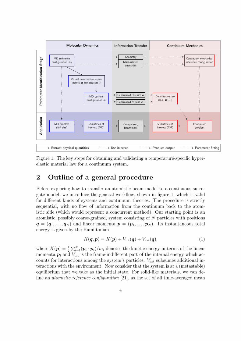
Figure 1: The key steps for obtaining and validating a temperature-specific hyper-elastic material law for a continuum system.

2 Outline of a general procedure

Before exploring how to transfer an atomistic beam model to a continuous surro-gate model, we introduce the general workflow, shown in figure 1, which is validfor different kinds of systems and continuum theories. The procedure is strictlysequential, with no flow of information from the continuum back to the atom-istic side (which would represent a concurrent method). Our starting point is anatomistic, possibly coarse-grained, system consisting of N particles with positionsq = (q1, . . . , qN) and linear momenta p = (p1, . . . ,pN). Its instantaneous totalenergy is given by the Hamiltonian

H(q,p) = K(p) + Vint(q) + Vext(q), (1)

where K(p) = 12

∑Ni=1(pi · pi)/mi denotes the kinetic energy in terms of the linear

momenta pi and Vint is the frame-indifferent part of the internal energy which ac-counts for interactions among the system’s particles. Vext subsumes additional in-teractions with the environment. Now consider that the system is at a (metastable)equilibrium that we take as the initial state. For solid-like materials, we can de-fine an atomistic reference configuration [21], as the set of all time-averaged mean

4

positions in the initial state:

A0 =¶Qi | i = 1, . . . , N

©, Qi := 〈qi〉. (2)

Now suppose that we represent the system using a still-undetermined continuumtheory, in which each continuum point is underlaid with a local thermodynamicsystem having n kinematic state variables or generalized strainsK = (K1, . . . , Kn).In three-dimensional continuum mechanics these would usually correspond to, forexample, the n = 6 stretch components of the deformation gradient F . These arealso represented by the stretch tensor U of the polar decomposition F = RU.Frame-indifference implies the thermodynamic system is independent of the threerotatory components of R.

Our goal is a continuum mechanical surrogate model for atomistic problemsrepresenting quasi-static processes at constant temperature and with a fixed num-ber of particles. Thus, a new atomistic state is obtained by a series of smallperturbations of the boundary conditions in an NV T ensemble and subsequentequilibrations, corresponding to applications where observation times are longerthan equilibration times and in particular longer than the time needed for anyviscous processes. This suggests that it is sufficient to consider the functional re-lationship ψ = ψ(X,K, T ) between the kinematic state and the Helmholtz freeenergy per unit mass at (quasi-)equilibrium, and to assume that the associatedthermodynamic tensions or generalized stresses are given by

κ(X,K, T ) =∂

∂Kψ(X,K, T ), (3)

which could, for example, correspond to the first Piola-Kirchhoff stress (dividedby reference mass density). The possibility of an explicit dependence of the con-stitutive relations on the position is indicated by X, which specifies a materialpoint in the reference configuration for a suitable coordinate system. In the three-dimensional case, this corresponds to a material coordinate X, in which case weuse a bold face symbol. It is known from statistical mechanics that the absoluteHelmholtz free energy of a system at equilibrium with a homogeneous kinematicstate K is

Ψ = Ψ(K, T ) = −kBT lnZ(K, T ), (4)

where the canonical partition function is given by

Z(K, T ) =1

h3NN1! · · ·Ns!

∫P(K)

expÄ−H(q,p)/kBT

ädqdp (5)

with a total of N = N1 + · · · + Ns particles of s different species [30]. The phasespace P(K) ∈ R6N containing elements (q,p) is chosen to contain the atomic

5

positions consistent with K; usually no restrictions are placed on the momenta.This establishes the connection between the atomistic degrees of freedom and themacroscopic free energy. It is clear that the 6N -fold integral in (5), as well aspartial derivatives of Ψ or of the density ψ usually cannot be evaluated in closedform. Fortunately, these derivatives, such as stresses, can be approximated as timeaverages using MD.

The main task now is to determine the stress-strain relationship between κ andK in (3). We proceed as follows. Suppose that the atomic reference configurationA0 represents a calibration system used only to obtain the desired constitutiverelation. A0 may be much smaller than the system sizes of the target applications,but is still large enough for adequate statistical sampling.

We define a set of virtual deformation experiments (VDE), a set of boundaryconditions applied to A0 that drive the system to a deformed configuration A. Theboundary conditions are quite arbitrary and could consist of, for example, displac-ing a subset of boundary atoms to a prescribed location or exerting additionalforces on all or parts of the atoms. To mimic an isothermal deformation processat this stage, the displacements or forces of the VDEs are first imposed slowlyand are followed by sufficient additional equilibration time. Another requirementis that the boundary conditions are chosen so that they neither restrict nor de-flect the particles’ movement in some inner region of the calibration system. Thus,when we determine values for the generalized stresses κ from the atomistic system,all thermal vibrations are taken into account. For example, the virial expressionfor the Cauchy stress [31] requires averaging over the individual linear momentaassociated with the currently deformed state.

Finally, if we can also obtain expressions for the strains K based on the atom-istic trajectories, we can carry out a parameter-fitting procedure to obtain a func-tional relationship such as (3). The method for obtaining generalized stressesand strains from atomistic simulations must be developed for each continuumtheory that we want to use, as shown in the following section for geometricallyexact beams. Another scenario which fits into this abstract workflow is provided inSchmidt et al. [25], which analyzes a three-dimensional polymeric system for whichthe stress-strain relationship cannot be obtained using a classical representativevolume element.

The remaining steps in the workflow are the transfer of the initial geometry ofA0 to the continuum mechanical model and the determination of quantities relatedto the masses of the atoms, such as mass density or inertia tensors. We referto the constitutive law, together with this information, as the surrogate model.Afterwards, we can apply the constructed model. To validate our procedure, weset up a benchmark problem in section 4.1 at both atomistic and continuum scales,and then compare several resulting quantities of interest extracted from each test

6

case. Problem details such as the applied loading conditions are independent of themodel construction stage. We do not expect to observe exact agreement in thesecomparisons as homogenized continuum descriptions are obtained and atomisticdetails are irrecoverably lost. Nevertheless, an approximate descriptions of thematerial behavior of nanoscale beams is very useful for applications involving one ormore such beam structures, which may be larger or made of varying materials. Alsofor coupled methods that concurrently handle atomistic and continuum domains,one may need a reliable material description for the latter.

3 A surrogate model for beam-like atomic struc-

tures

We now set up a continuum mechanical surrogate model for atomic beam-likestructures using the workflow outlined in section 2. This procedure can be adaptedto any simulation where ordinary bulk representative volume elements cannot beconstructed. The latter usually require full three-dimensional periodicity, so that amacroscopic strain F can be directly applied to the atomistic system, and stressescan be averaged over the whole domain. To overcome this restriction, we use anindirect approach, relating simultaneously determined stresses and strains in a setof deformed states for a calibration system which is as small as possible but stilllarge enough to exhibit representative behavior. However, in the case of beams,the cross section used must be the same as in the intended application problem,since the extracted material properties strongly depend on the beam cross section.

3.1 Geometrically exact beams

We briefly present the main aspects of geometrically exact beams, adapted fromAntman [32], Simo [9], and [10]. A beam is a slender three-dimensional body withstress-free reference configuration B0 and deformed current configuration B. Theformer is given as a line of centroids R(S), parameterized with respect to the arclength: |R′| ≡ 1. Here, S ∈ I = [0, L], where L is the total arc length. At everyposition S there is a circular cross section1 C = ζ ∈ R2 | ‖ζ‖ ≤ Rcs of radius Rcs.The cross sections’ orientation in space is described through the plane spanned bytwo orthonormal director vectors Dα(S), α = 1, 2, which can vary over I. If wedefine the domain P = C × I, the reference configuration can be parameterizedthrough the mapping

Φ : P → B0, (ζ, S) =Äζ1, ζ2, S

ä7→ R(S) + ζαDα(S), (6)

1In general, there are no special requirements for the shape of the cross sections, nor mustcross sections be identical at each arc length.

7

Figure 2: Schematic of a geometrically exact beam. Two exemplary cross sectionsare shown, through which the central line r (black) passes. Also shown are thethree director vectors d1 (cyan), d2 (white), d3 (red).

where Einstein summation is implied for Greek index α = 1, 2. At time t, thecentral line and directors attain new values r(S, t) and dα(S, t), respectively, whichform the parameterization for the current configuration:

ϕ : P × [0,∞)→ B, (ζ, S, t) 7→ r(S, t) + ζαdα(S, t) (7)

The current directors dα are still orthonormal and describe an undistorted, planarcross section. One can thus obtain complete orthonormal bases by defining D3 :=D1 × D2 and d3 := d1 × d2. These can be arranged as second-order tensorsindicating the change of the moving director bases,

Λ0(S) = Di(S)⊗Ei (8)

Λ(S, t) = di(S, t)⊗Ei. (9)

with summation over the Latin index i = 1, 2, 3. A schematic illustration of sucha beam is shown in figure 2. The composition

χ(·, t) = ϕ(·, t) Φ−1 : B0 → B (10)

is then the usual deformation mapping from three-dimensional continuum mechan-ics. Substituting it into the balance equations of linear and angular momentumyields the governing equations for the beam, which are now reduced to one spatialdimension:

n′(S, t) + n(S, t) = M0(S)r(S, t) (11a)

m′(S, t) + r′(S, t)× n(S, t) + m(S, t) = π(S, t), (11b)

where n is the stress-resultant force, m is the stress-resultant moment acting on across section, n and m are distributed external forces and torques per unit length,and where primes and dots denote partial derivatives with respect to S and t,

8

respectively. Conservation of mass is also presumed. Furthermore, we introduce

π(S, t) = iρ(S, t)w(S, t) (angular momentum of cross section)

(12)

iρ(S, t) = Mαβ2 (S)[δαβI − dα(S, t)⊗ dβ(S, t)] (spatial inertia tensor) (13)

w(S, t) = axÄΛ(S, t)Λ(S, t)T

ä(angular velocity vector) (14)

where ax(·) returns the axial vector of a skew-symmetric second-order tensor. Fi-nally we introduce the zeroth, first and second moments of mass of the crosssection

M0(S) =∫Cρ0(ζ, S) dζ, (15)

Mα1 (S) =

∫Cζαρ0(ζ, S) dζ, (16)

Mαβ2 (S) =

∫Cζαζβρ0(ζ, S) dζ, (17)

for the reference mass density ρ0(ζ, S). These can be interpreted as mass density,centroid and moment of inertia of the cross section, respectively. For simplicity,(11) already assumes that Mα

1 ≡ 0 for α = 1, 2. The unknowns are the centralline r and the rotation Λ. The stress-resultant force n and moment m act asgeneralized stresses, and are obtained as partial derivatives of the free energy. Thekinematic descriptors are given by the following strain measures [33]:

Γ = ΛT r′ −ΛT0 R′ (18a)

Ω = axÄΛTΛ′ −ΛT

0 Λ′0ä, “Ω = ΛTΛ′ −ΛT

0 Λ′0, (18b)

where · gives the skew-symmetric tensor for a given axial vector. The first strain Γcaptures shear and axial extension, while Ω is associated with bending and twist-ing. Obviously, this formulation neglects possible changes in the cross-sectionalshape, such as warping or ovalization, although extensions exist to account forthese [34–39]. This typically leads to additional kinematic descriptors which mustobey additional balance laws. However in the standard case as described above,the constitutive relations are given for the material counterparts N, M of forceand moment:

n = ΛN, N = ∂Γψ(S,Γ,Ω) (19a)

m = ΛM, M = ∂Ωψ(S,Γ,Ω) (19b)

Our main task is to determine the Helmholtz free energy (per unit reference length)ψ. Numerical treatments of the PDE system (11) have been thoroughly studied

9

[40–45]. One particular problem here is the proper representation and integrationof the rotation, which must remain in SO(3) and be adequately interpolated at thequadrature points [46]. The most frequently used approach is a quaternion-basedformulation [40, 47–49]. We base our implementation on the work of Celledoniand Safstrom [50].

3.2 Transfer of geometry and mass-related quantities

Given an atomistic reference configuration A0 of initial mean positionsQi, the firsttask in parameterizing the continuum model is to determine the initial position ofthe line of centroids R(S) and the moving basis of directors Λ0(S), S ∈ I. Weassume that the reference line of centroids is aligned along the z-axis, R(S) =S · E3, S ∈ I, and that the directors have no initial rotation, Λ0 ≡ I. We callthis the canonical reference configuration shown in figure 6a. To approximatelyreconcile a set of given initial positions Qi with this assumption, we identify arigid transformation

T (X) = SX +C, S ∈ SO(3),C ∈ R3, (20)

that satisfies the following requirements when applied to the mean positions Qi:

1. The z-axis is chosen to be the axis line of the slenderest cylinder containing allreference mean positions Qi, so that the transformed reference configurationT (A0) lies along the z-axis. The beam’s length L is then the difference ofthe largest and smallest z components.

2. The transformed cross section centroids should, on average, lie on the z-axis:

〈Mα1 〉I =

1

L

∫IMα

1 (S) dS!

= 0, α = 1, 2 (21)

3. The principal axes of inertia of the transformed cross sections should, onaverage, be aligned along the x- and y-axes:¨

M122

∂I =

¨M21

2

∂I =

1

L

∫IM12

2 (S) dS!

= 0 (22)

The calibration system is chosen large enough so that the average moments ofmass are statistically representative along the central line. Thus, material in-homogeneities need not be resolved, and the moments of mass can be taken asconstant. In an application problem, the beam’s material properties can of coursevary over certain regions, each of which is parameterized based on different calibra-tions. An appropriate transformation T can be found, for example, using Matlab’s

10

Optimization Toolbox [51]. From here on, without loss of generality, we take T tobe the identity map to avoid having to transform the vectorial and tensorial quan-tities needed for subsequent calculations. For a canonical reference configuration,the strain measures (18) become

Γ = ΛT r′ −E3 (23a)

Ω = axÄΛTΛ′

ä, “Ω = ΛTΛ′ (23b)

3.3 Virtual deformation experiments

We now want to drive the atomistic system into a state as homogeneously deformedas possible. As will be shown in section 3.5, the generalized stress measures n,mcan be obtained from phase averages. Since these are approximated as time av-erages in MD, to properly sample phase space the atomic positions and momentamust be consistent with an isothermal (NV T ) ensemble. In particular, the trajec-tories must be representative for the imposed kinematic state and thus must beallowed to freely explore the corresponding restricted phase space. The only con-straint we apply is to prescribe positions for a set of boundary atoms ∂A0 ⊂ A0 atthe free ends and, to produce sheared configurations, sometimes along thin stripeson the beam’s lateral surface. In particular, we impose a pair of target strains(Γ0,Ω0) exactly at all boundary atoms Qi ∈ ∂A0. These boundary displacementsare applied slowly over time, starting at the initial positions Qi and finishing atend positions given by the target strain. In our simulations, this is carried out over1 ns, followed by 1 ns of additional equilibration and finally 2 ns of actual samplingof the generalized stresses and strains in the now deformed state.

We derive the necessary displacements from the analytical description of acontinuum system that is homogeneously deformed as Γ0 and Ω0 everywhere.First, (23a) yields

r′(S) = Λ(S) · (Γ(S) +E3); (24)

from (23b), we obtainΛ′(S) = Λ(S) · “Ω(S). (25)

For an initial central line position rin and an initial rotation Λin at S = 0, weobtain a system of ordinary differential equations for r and Λ:

r′(S) = Λ(S) · (Γ0 +E3), r(0) = rin (26a)

Λ′(S) = Λ(S) · “Ω0, Λ(0) = Λin (26b)

11

Here, (26b) is uncoupled and immediately yields Λ(S) = Λin expÄS · “Ω0

ä. We can

then integrate (26a) to obtain

r(S) = rin + Λin

ñ∫ S

s=0expÄs · “Ω0

äds

ô· (Γ0 +E3). (27)

This integration can readily be carried out (Appendix A). For a beam whose endat S = 0 coincides with the canonical reference configuration we have r0 = 0 andΛ0 = I. To facilitate subsequent parameter fitting, we are especially interested inpure strain states, where only one of the six strain components is non-zero. Forexample, pure bending about the x-axis, Γ0 = [0, 0, 0], Ω0 = [Ω1, 0, 0], is describedin component form as

r(S) =

01

Ω1(cos(S · Ω1)− 1)

1Ω1

sin(S · Ω1)

, Λ(S) =

1 0 00 cos(S · Ω1) − sin(S · Ω1)0 sin(S · Ω1) cos(S · Ω1)

. (28)

Solutions for the remaining pure deformations are given in Appendix A. We havenow identified the exact configuration that a continuum beam with a homogeneousstrain would occupy. To obtain a candidate equilibrium state at finite temperaturewith approximately the same strain from an MD simulation, we must prescribethis configuration at the boundary particles of the atomistic beam. To inducea realistic deformation, we carry this out slowly over some time span te. Thecorresponding interpolation rules in time are given by:

r(S, t) =1

te

Ä(te − t) ·R(S) + t · r(S)

ä=te − tte·

00S

+t

te· r(S), (29)“Λ(S, t) = Λ0

ÄΛT

0 Λ(S)ä tte = Λ(S)

tte (30)

From these quantities we can set up the deformation mapping as“ϕ(ζ, S, t) = r(S, t) + ζαdα(S, t), (31)

with the directors dα extracted from “Λ. Now assume that an atom to be movedis initially at position Q and belongs to the continuum reference configuration, inwhich it has coordinates Φ(ζ, S) = Q. The actual displacement of the atom2 istherefore

∆“ϕ(ζ, S, t) := “ϕ(ζ, S, t)−Φ(ζ, S). (32)

2In practice, the actual mean positions Q of the boundary atoms are not deformed. Instead,their positions Q in the last timestep of the equilibration of the reference configuration are takenas the starting point.

12

Figure 3: The six pure deformation modes of a geometrically exact beam, appliedto an atomistic model of a nanowire.

Since the reference configuration is canonical, (ζ1, ζ2, S) = (Q1, Q2, Q3) and thuswe can express the displacement in terms of the atomic coordinates,

∆ϕ(Q, t) := ∆“ϕ(Q1, Q2, Q3, t) = “ϕ(Q1, Q2, Q3, t)−Q. (33)

which is suitable for implementation, as it can be evaluated for any given atom-istic coordinate using (31). In figure 3, a sample nanowire is shown after beingdeformed to each of the six pure strain states. Finally, we note that prescribingpositions for a boundary region ∂A0 does not cause the mean positions of the free-moving atoms to exactly attain those particular strain values. We merely imposethe displacement to obtain candidates for deformed systems, from which we candetermine the actually occurring local stresses and strains.

3.4 Generalized strain measures from atomistic simula-tions

Stresses and strains may be distributed non-homogeneously along the deformedbeam. Therefore, we subdivide the beam along its arc length into a number ofsmall segments Ij, j = 1, . . . , Nseg, of length ∆S = L/Nseg. A sample nanowirewith a highlighted segment is shown in figure 4. The set of atoms corresponding tosegment j in the reference configuration is denoted A0,j. The new mean positionsafter deformation are called the current atomistic configuration:

A = qi | i = 1, . . . , N , qi := 〈qi〉, (34)

13

where the time average is taken after equilibration with the applied deformationboundary conditions. From the position changes of the atomic mean positionsfrom Qi to qi, i ∈ A0,j, we want to deduce the continuum strain measures Γ andΩ. To this end, we construct an approximation χj for the continuous deformationmap χj in segment j that interpolates the discrete displacement information byusing the linear ansatz

q = χj(Q) ≈ χj(Q) := FjQ+ cj (35)

and determine Fj and cj from the following least-squares problem [cf. 25]:

1

2

∑i∈A0,j

∥∥∥χjÄQi

ä− qi

∥∥∥2=

1

2

∑i∈A0,j

∥∥∥FjQi + cj − qi∥∥∥2 !

= minFj ,cj

. (36)

If atomic masses differ, a weighted cost function can be used. Similar choices fordescribing local atomic deformations are given in Horstemeyer and Baskes [52] andZimmerman et al. [53, 54]. Since ∂Qχj ≈ Fj, the second-order tensor Fj playsthe role of an approximate deformation gradient. From (7) and (10), the actualdeformation gradient of a geometrically exact beam is given by

F (ζ, S) = d1(S)⊗ E1 + d2(S)⊗ E2 +ϕ′(ζ, S)⊗ E3. (37)

Forming weighted averages of dα and r′ over the beam segment domain C × Ijyields

dα := 〈dα〉C×Ij =

∫C×Ij dα(S)ρ0(ζ, S) dζdS∫C×Ij ρ0(ζ, S) dζdS

=

∫Ij dα(S)M0(S) dS∫Ij M0(S) dS

=1

∆S

∫Ijdα(S) dS (38a)

r′ := 〈r′〉C×Ij =

∫C×Ij r′(S)ρ0(ζ, S) dζdS∫C×Ij ρ0(ζ, S) dζdS

=1

∆S

∫Ij

r′(S) dS, (38b)

since M0 is a constant along the entire calibration system. At the same timeMα

1 ≡ 0 and thus

〈ζαd′α〉C×Ij =

∫C×Ij d

′α(S)ζαρ0(ζ, S) dζdS∫

C×Ij ρ0(ζ, S) dζdS=

∫Ij d

′α(S)Mα

1 (S) dS∫Ij M0(S) dS

= 0. (39)

Hence, the averaged deformation gradient follows from (37) as

F j := 〈F 〉C×Ij = 〈d1〉C×Ij ⊗ E1 + 〈d2〉C×Ij ⊗ E2 + 〈r′ + ζαd′α〉C×Ij ⊗ E3

= d1 ⊗ E1 + d2 ⊗ E2 + r′ ⊗ E3. (40)

14

Figure 4: Silicon nanowire with a highlighted beam segment, indicating a partic-ular selection of atoms.

Equating the least-squares deformation gradient Fj with (40) yields, in matrixform,

[Fj]!

=îF j

ó=îd1,d2, r′

ó(41)

so the columns of [Fj] are just the averages of the directors and tangent vectorof the central line defined above. Although the directors dα at specific locations(ζ, S) are orthonormal, this need not hold for the averaged versions dα. However,we make this very assumption a priori and solve the minimization problem (36)under the constraint dα · dβ = δαβ. This is reasonable for relatively small beamsegment lengths ∆S ≈ 10 A. This allows us to define a completed director basisfor segment j as Λj :=

îd1,d2,d3 = d1 × d3

ó. Using (23), the strain measures on

beam segment j can be defined based on (40) as

Γj := ΛTj r′ − E3, (42)

Ωj := axÄΛTj Λ′j

ä, (43)

where the spatial derivative Λ′j is obtained via ordinary finite differences, althoughthis could be improved by a more suitable approximation scheme for orthogonalmatrices.

3.5 Generalized stress measures from atomistic simulations

We still need to determine the forces n and moments m acting on cross sectionsof the beams from virtual deformation experiments. According to Simo [9], thefollowing relationship holds:

n(S) =∫CP (ζ, S)E3 dζ =

∫Cσ(ζ, S)d3(S) dζ, (44)

where P is the first Piola-Kirchhoff stress and σ denotes the Cauchy stress, andthe last equality follows from (37). We denote by rj the centroid of deformedsegment j and make the rather coarse approximations

σ(ζ, S) ≈ σ(rj), d3(S) ≈ d3 (45)

15

throughout segment j. Hence (44) yields an approximate expression for the normalforce in segment j:

nj :=∫Cσ(rj)d3 dζ = R2

csπ · σ(rj)d3 (46)

There are several methods for connecting the Cauchy stress to atomistic simu-lations [31]. To define a localized stress around the spatial point x, a commonapproach is to use a virial stress expression such as

σV (x) =1

vol(Nx)

∑i∈Nx

σVi , (47)

where Nx is a suitable neighborhood of x, and σVi are the per-atom virial stressesof the atoms in this neighborhood, which involves the instantaneous particles’positions qi and linear momenta pi as well as the forces fi acting on them, all ofwhich appear in the time average at equilibrium:

σVi =

Æ−Çpi ⊗ pimi

+ fi ⊗ qiå∏

(48)

Expression (47) for the stress tensor in three dimensions can be obtained by takingthe derivative of (4) with respect to the state variable F [55]. We choose the setA,j to be the neighborhood Nrj of x = rj. This neighborhood spans the linearlytransformed reference segment domain ϕj(C × Ij), ϕj = χj Φ, resulting in avolume of R2

csπ ·∆S · detFj. Combining this with (46), we arrive at

nj =1

∆S · detFj

∑i∈A0,j

σVi · d3. (49)

This gives us the first of two required generalized stress measures. The other isthe moment acting on a cross section,

m(S) =∫C(ϕ(ζ, S)− r(S))× σ(ζ, S)d3(S) dζ (50)

=∫Cζαdα(S)× σ(ζ, S)d3(S) dζ (51)

= dα(S)×ï∫Cζασ(ζ, S) dζ

òd3(S). (52)

To evaluate the integral in brackets, we partition the cross section into an over-lapping grid of Nh × Nh smaller squares C(a,b), each of side length ∆ζ and with

16

midpoint ζ(a,b):

∫Cζασ(ζ, S) dζ =

Nh/2−1∑a=−Nh/2

Nh/2−1∑b=−Nh/2

∫C(a,b)

ζασ(ζ, S) dζ (53)

.= (∆ζ)2

Nh/2−1∑a=−Nh/2

Nh/2−1∑b=−Nh/2

ζα(a,b)σVÄζ(a,b), S

ä=: mj (54)

In subsequent computations, we chose Nh = 20. Using (47) again, we evaluateσVÄζ(a,b), S

äfor a now smaller neighborhood CV(a,b) × Ij, where CV(a,b) is a possibly

different portion of the cross section used in the stress calculation:

σVÄζ(a,b), S

ä=

1

detFj · areaÄCV(a,b)

ä·∆S

∑i|Qi∈Φ

ÄCV(a,b)×IjäσVi (55)

Finally, using (19), we obtain the corresponding material quantities

Nj := ΛTj nj, Mj := ΛT

j mj. (56)

This and the preceding section provide the means that are necessary to bring inaccordance the various quantities calculated for an equilibrated, deformed state ofthe atomistic beam with an assumed coinciding continuum beam. For the latter wecan hence determine the local strains and stresses within each arc length segmentIj.

3.6 Fitting of the energy density

We now must fit the energy density function, for which we make the quadraticansatz

ψ(Γ,Ω) =1

2Γ ·CNΓ +

1

2Ω ·CMΩ,

CN = diag(GA1, GA2, EA), (57)

CM = diag(EI1, EI2, GJ), (58)

where CN contains shear stiffnesses and axial stiffness and CM contains bendingstiffnesses and torsional stiffness. We use the term “stiffness” for mere material-specific properties such as EA; in a different context it could in addition be dividedby a geometric quantity such as the beam length. The resulting generalized stressesthen have the form

N(Γ,Ω) = ∂Γψ(Γ,Ω) = CNΓ, (59a)

M(Γ,Ω) = ∂Ωψ(Γ,Ω) = CMΩ. (59b)

17

Though simple, this completely uncoupled choice for the stress-strain relationshiphas proven very useful and is employed throughout the literature [40]. Of course,more elaborate functional forms can be used without affecting the essential fittingprocedure. For general materials, however, about which we have no prior infor-mation on additional deformation modes, a quadratic energy function typically isa suitable guess. Even for large beam deflections, the local stress-strain relation-ship can usually be well approximated as linear. If additional knowledge on thematerial at hand is available and a suitably adapted energy function is known, itcan be fitted in the same manner. In these cases, however, new VDEs should beintroduced to trigger the additional modes, as in section 3.3.

The procedures described in sections 3.4 and 3.5, yield material stress-strainquadruples

(Γ

(k)j ,Ω

(k)j ,N

(k)j ,M

(k)j

)for each segment and for a larger set of virtual

deformation experiments (VDE) with index k = 1, . . . , Nvde. If we arrange the sixunknown material properties from (58) as a vector λ ∈ R6 we obtain the followingobjective function to fit these unknowns:

g(λ) :=1

2

Nvde∑k=1

Nseg∑j=1

Å ∥∥∥N(k)j −N(Γ

(k)j ,Ω

(k)j )

∥∥∥2+∥∥∥M(k)

j −M(Γ(k)j ,Ω

(k)j )

∥∥∥2ã

(60)

=1

2

Nvde∑k=1

Nseg∑j=1

Å ∥∥∥N(k)j −CNΓ

(k)j )

∥∥∥2+∥∥∥M(k)

j −CMΩ(k)j )

∥∥∥2ã

(61)

Minimization of g yields the sought material-specific stiffnesses. Since the partialderivatives of ψ are fully decoupled and since, by construction of the virtual ex-periments, we expect only one component of (Γ,Ω) to deviate significantly fromzero, it makes sense to fit each parameter λi individually: for example,

g(EA) = g(λ3) =1

2

∑k

∑j

(N

(k)j,3 − λ3 Γ

(k)j,3

)2(62)

By eliminating the noise in the remaining stress and strain components the valueof the final fitted parameter can usually be stabilized. Here, k runs only over thoseVDEs designed to excite the corresponding deformation mode.

4 Numerical results

We now present, as a benchmark, a direct comparison between purely atomisticand continuum mechanical simulations. We do not distinguish between calibra-tion and full system; material parameters are determined for the same systemsize used for the benchmark calculations. The MD simulations have been per-formed using LAMMPS [56], while the finite element code for the beam model

18

has been implemented based on the libMesh library [57]. Specifically, for a siliconnanowire and a carbon nanotube we perform Nvde = 30 virtual experiments withstrain components Γi = 0.02, 0.04, . . . , 0.10 and Ωi = 2× 10−4 A−1, 5× 10−4 A−1,8× 10−4 A−1, 0.001 A−1, 0.002 A−1 for i = 1, 2, 3. These choices are representativeas guidelines for the choice of VDEs. The values of Γi and Ωi should be restrictedto the range of deformations that can be represented by the chosen functionalform for the energy density ψ. In the case of (58) this means that the stress-strainrelationship should remain linear. A possibly larger range may be included whena nonlinear relationship is assumed. By inspection of the input data generated bythe VDEs one can exclude cases that cannot be properly captured by the chosenfunctional form.

Furthermore, we usually exclude some beam segments close to the boundarywhere atom positions are fixed and computed stresses are not meaningful. We alsonote that a simple hyperelastic material model like (58) can only be fitted to acertain range of deformations, as dictated by the virtual deformation experimentsused, though extensions to overcome this issue could be conceived.

4.1 Contact with a Lennard-Jones wall

An atomistic beam is initially aligned along the z-axis from X3 = 0 to X3 = L.A small set ∂A0 of atoms near the origin is kept fixed. We then introduce a half-space E− of Lennard-Jones (LJ) particles separated from the beam by a plane Ewith outer unit normal ν ∈ R3 and distance −d from the origin. The half-spacecontaining the LJ particles is then given by

E− =¶y ∈ R3 | y · ν − d < 0

©, (63)

while the beam and origin are located in the complementary half-space

E+ =¶y ∈ R3 | y · ν − d > 0

©. (64)

The distance dE(y) = y·ν−d partitions R3 into E, E−, and E+. Although infinite,E− can be seen as a good approximation to a large rigid body that interacts withthe beam via a LJ potential. As it is not itself deformed, E− is is not an explicitpart of our model; only its interactions with the beam are. The wall can bepushed towards the beam, which is still fixed at one end, as shown in fig. 5. Thusd increases over multiple displacement steps. As a result, the beam undergoes asubstantial deflection away from the wall but always remains in E+. The potentialenergy of the entire wall interacting with a particle at position x ∈ E+ is an infinitesum over all pairwise LJ interactions, which have the form:

φ(r) = 4ε

ñÅσr

ã12

−Åσr

ã6ô

(65)

19

Figure 5: Illustration of a geometrically exact beam, 1. in its undeformed referenceconfiguration and 2. after coming into contact with a rigid Lennard-Jones wall.

Similar to [58], we approximate this summation through an integral over a contin-uum of LJ sites with constant particle density βw,

πw(x) =∫E−

βw · φ(‖y − x‖) dy (66)

=2

3πβwεσ

3︸ ︷︷ ︸=:ε

[2

15

Çσ

dE(x)

å9

−Ç

σ

dE(x)

å3]

= φ93( dE(x) ), (67)

resulting in the so-called Lennard Jones 9-3 potential

φ93(dE) = ε

[2

15

Çσ

dE

å9

−Çσ

dE

å3], (68)

which is a function only of the distance dE of the particle from plane E. Theseinteractions can be easily modeled using LAMMPS.

We now turn to the continuum framework and determine the total interactionenergy between this wall and a deformed configuration ϕ of the geometricallyexact beam. To this end, we introduce the contact energy, which weights allparticle interactions with the wall by the current particle density of the beam,β(x):

Πc[ϕ] =∫Bβ(x)πw(x) dx =

∫C

∫Iβ(ϕ(ζ, S))πw(ϕ(ζ, S)) |detDϕ(ζ, S)| dζdS

(69)

We define the transformed particle density

β(ζ, S) := β(ϕ(ζ, S)) |detDϕ(ζ, S)| = β0(Φ(ζ, S)) (70)

and make the simplifying assumption for the reference particle density β0(X) that∂Xα β0 ≡ 0, α = 1, 2, yielding β = β(S) and hence

Πc[ϕ] =∫Iβ(S)

∫Cπw(r(S) + ζαdα(S)) dζ dS. (71)

20

We can evaluate the inner integral of (71) analytically at a specific arc-lengthposition S:∫Cπw(r + ζαdα) dζ =

2

15εσ9

∫CdE(r + ζαdα)−9 dζ − εσ3

∫CdE(r + ζαdα)−3 dζ

(72)

=2

15εσ9 · J9(dE(r),ν ·Qd1, Rcs)− εσ3 · J3(dE(r),ν ·Qd1, Rcs),

(73)

for an appropriately chosen3 orthogonal transformation Q and

J9(a, b, R) =R2π

64· 5b6R6 + 120a2b4R4 + 240a4b2R2 + 64a6

(a−Rb)15/2(a+Rb)15/2, (74)

J3(a, b, R) =R2π

(a−Rb)3/2(a+Rb)3/2. (75)

The details of this calculation are deferred to B. A similar procedure might alsobe feasible to find a closed-form expression for the LJ interaction between twocircular cross sections, which could be used to simplify the computation of thecontact energy between two beams. If the assumption β(ζ, S) ≡ β(S) is violated,the relationship (71) can be generalized straight-forwardly if the particle densityβ is piecewise constant within a number Nann of concentric annuli of radii 0 =Rcs,0 < Rcs,1 < · · · < Rcs,Nann = Rcs. In this case, the integral over a single annulusis obtained by subtracting the expression for a disk with radius Rcs,i−1 from thatfor Rcs,i. On the other hand, the continuum problem that we want to solve is tominimize the energy functional

Π[ϕ] := Πint[ϕ] + Πc[ϕ], Πint[ϕ] :=∫IψÄΓ[ϕ](S),Ω[ϕ](S)

ädS, (76)

subject to fixed boundary conditions at S = 0. The relevant thermodynamicpotential for isothermal conditions is the Helmholtz free energy, whose internalpart is given by Πint. Πc actually denotes only the potential energy of the wall–beam interaction, since it seems unfeasible to devise a proper model for the freeenergy of the interaction with a wall (given in terms of ν and d). We thereforeconsider Πc as a suitable approximation for the latter.

We now carry out a fully atomistic simulation of a beam interacting with anapproaching LJ wall. At equilibrium, we extract certain quantities of interestand compare them to their continuum equivalents obtained from finite element

3See B. The symbol Q for the orthogonal transformation is not to be confused with the atomicpositions.

21

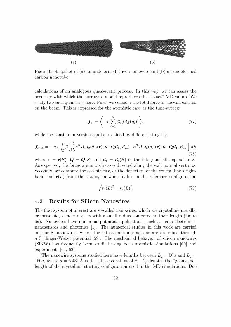
(a) (b)

Figure 6: Snapshot of (a) an undeformed silicon nanowire and (b) an undeformedcarbon nanotube.

calculations of an analogous quasi-static process. In this way, we can assess theaccuracy with which the surrogate model reproduces the “exact” MD values. Westudy two such quantities here. First, we consider the total force of the wall exertedon the beam. This is expressed for the atomistic case as the time-average

fat =

⟨−ν

N∑i=1

φ′93(dE(qi))

⟩, (77)

while the continuum version can be obtained by differentiating Πc:

fcont = −ν ε∫Iβï 2

15σ9·∂aJ9(dE(r),ν ·Qd1, Rcs)−σ3·∂aJ3(dE(r),ν ·Qd1, Rcs)

òdS,

(78)where r = r(S), Q = Q(S) and d1 = d1(S) in the integrand all depend on S.As expected, the forces are in both cases directed along the wall normal vector ν.Secondly, we compute the eccentricity, or the deflection of the central line’s right-hand end r(L) from the z-axis, on which it lies in the reference configuration:√

r1(L)2 + r2(L)2. (79)

4.2 Results for Silicon Nanowires

The first system of interest are so-called nanowires, which are crystalline metallicor metalloid, slender objects with a small radius compared to their length (figure6a). Nanowires have numerous potential applications, such as nano-electronics,nanosensors and photonics [1]. The numerical studies in this work are carriedout for Si nanowires, where the interatomic interactions are described througha Stillinger-Weber potential [59]. The mechanical behavior of silicon nanowires(SiNW) has frequently been studied using both atomistic simulations [60] andexperiments [61, 62].

The nanowire systems studied here have lengths between Lg = 50a and Lg =150a, where a = 5.431 A is the lattice constant of Si. Lg denotes the “geometric”length of the crystalline starting configuration used in the MD simulations. Due

22

to thermal fluctuations, the atomistic reference configuration A0 typically deviatesfrom this perfectly straight shape, leading to different effective lengths L. Threecross sections were chosen as circular (001) surfaces with atoms located withindifferent radii of Rg = 2.5a, Rg = 3.5a and Rg = 4.5a, which are also merelygeometric. Physically, though, the atoms are not point particles, but have a finiteextent; for example, the van der Waals radius of Si is Rvdw = 2.1 A. Therefore, theeffective cross-sectional radius is Rcs = Rg +Rvdw. The Lennard-Jones parametersof the wall interaction were set to ε = 600 A3 bar and σ = 3.5 A, and the wall was

tilted against the z-axis, ν =î0, 0.3,−

√0.91

óT.

The identified mass-dependent properties for systems of different radius andlength are summarized in table 1. The temperature was always T = 300 K. We seethat the inertia is distributed symmetrically, as expected. The only exception is thevery slender nanowire (Rg = 2.5a, Lg = 150a), where the thermal vibrations leadto significant deviations in the atomic mean positions from a canonical referenceconfiguration even without any deforming boundary conditions applied, resultingin a seemingly asymmetric mass distribution. Averaging the atom positions overa longer time span may attenuate this issue. The material parameters determinedfor the constitutive law (58) are presented in table 2.

Rg Lg L [A] M0 [A−1 u] M112 [A u] M22

2 [A u]2.5a 50a 266 853 40 300 40 7002.5a 150a 798 851 52 000 41 3003.5a 60a 327 1580 141 000 141 0003.5a 150a 814 1580 141 000 141 0004.5a 150a 813 2640 394 000 394 000

Table 1: Silicon nanowires: The identified effective length L, mass density M0 andcross section inertia Mαα

2 , for various geometric dimensions Rg, Lg. Remark: 1 u= 1.66× 10−27 kg.

Rg Lg GA1 [A2bar] GA2 [A2bar] EA [A2bar] EI1 [A4bar] EI2 [A4bar] GJ [A4bar]2.5a 50a 2.37× 108 2.29× 108 4.09× 108 1.86× 1010 1.87× 1010 2.00× 1010

2.5a 150a 1.75× 108 1.68× 108 3.84× 108 1.67× 1010 1.83× 1010 1.80× 1010

3.5a 60a 4.67× 108 4.66× 108 9.31× 108 7.60× 1010 7.76× 1010 9.02× 1010

3.5a 150a 4.70× 108 4.62× 108 9.67× 108 6.86× 1010 7.39× 1010 8.84× 1010

4.5a 150a 8.34× 108 8.27× 108 1.58× 109 2.25× 1011 2.02× 1011 2.61× 1011

Table 2: Silicon nanowires: The identified material parameters for the constitutivelaw (58), for various geometric dimensions Rg, Lg. Remark: 1 A2 bar = 10−15 N,1 A4 bar = 10−35 Nm2.

23

pd GA1 [A2bar] GA2 [A2bar] EA [A2bar] EI1 [A4bar] EI2 [A4bar] GJ [A4bar]0% 4.67× 108 4.66× 108 9.31× 108 7.60× 1010 7.76× 1010 9.02× 1010

1% 4.75× 108 4.64× 108 8.50× 108 6.69× 1010 7.30× 1010 7.99× 1010

2% 4.25× 108 4.23× 108 7.55× 108 6.23× 1010 5.72× 1010 7.12× 1010

Table 3: Silicon nanowires: The identified material parameters for the constitutivelaw (58) for a system with Lg = 60a, Rg = 3.5a and vacancy percentages pd ofremoved atoms.

Dividing the axial stiffness EA by the cross-sectional area A = R2csπ gives the

axial Young’s modulus of the beam. For example, for beams of length Lg = 150aand radii Rg = 2.5a, 3.5a, and 4.5a we find E = 49.8 GPa, 69.1 GPa, and 71.3 GPa,respectively. These values are significantly smaller than Young’s modulus for bulkSi, which is 151.4 GPa for the Stillinger-Weber potential. This reveals a well-knownsize effect in the mechanical properties of nanowires, caused by non-negligiblesurface effects as the surface-to-volume ratio becomes large [63–66]. Thus, withouta rule for scaling the material properties between different radii (and possiblydifferent cross-sectional shape), one has to repeat the parameter identificationprocedure for each type of cross section.

The structures considered so far were constructed in a perfectly defect-freemanner. In reality, though, there is usually a certain amount of defects presentin the system. We can take this into account by identifying material parametersthat reflect a given statistical distribution of such defects. To this end, one can forexample build an initial configuration that contains vacancies, impurities etc. in aprescribed amount. The size of the calibration system then needs to be chosen largeenough such that it constitutes a representative sample of defect distribution. Likebefore, one has to keep in mind that the continuum material description cannotcapture plastic events. As the latter may be triggered more easily in the presenceof defects, the material parameters determined may only be valid for relativelysmall local strains.4 Table 3 shows the material parameters found for again aSiNW at T = 300 K with geometric dimensions Lg = 60a and Rg = 3.5a, butthis time with vacancy ratios pd = 0%, 1% and 2%. That is, a percentage pd ofatoms are randomly removed from the perfect nanobeam, followed by the usualconducting of the VDEs. The table demonstrates how the structural weakeningcan be quantified as more vacancies lead to a consistent decrease in the stiffnessvalues.

Figure 7 shows the y- and z-components of the force exerted by the LJ wallonto the beam over a displacement range of 35 A, where a displacement of zero

4In principle, within a concurrent multiscale method, one could alternatively also use a two-level approach that solves a microscale problem around each point defect [67].

24

corresponds to the wall having moved to the initial location of the free end of thebeam’s central line; an increasing value means that the wall has moved beyond thispoint to cause more deflection. Each of the eighty displacement steps consisted of0.4 ns of moving the wall by a small increment, another 0.4 ns of equilibration and0.4 ns of sampling. The shift between the continuum and atomistic curve is chosento yield good visual agreement; this implicitly determines the effective reach of thecontinuum beam within this contact problem. Error bars in the plot indicate thestandard deviation of ten repeated MD simulations, each performed with a varyingperturbation in the initial atomic velocities. We see that the trends of the forcesare well captured by the continuum model, where they remain within one standarddeviation from the atomistic mean values. However, we notice that the continuumforces contain a mild level of consistent underprediction with respect to the MDvalues. The error bars also show the fluctuation in the time-averaged atomisticforces increases as the wall approaches the beam. This can be explained by theincreasing number of beam atoms that interact with the wall, as each particleintroduces additional thermal fluctuations to the force (77). Also note that due to(77), (78) the two graphs are related to each other and differ only by the scalingof different components of ν. An enlarged image detail of the adhesive regime ofthe forces in y-direction is provided in figure 8.

The eccentricity, or the deflection of the beam’s end from the z-axis, is shownin figure 9 over a displacement range of 70 A. We still see qualitiative agreement,though the deflection is overestimated by the continuum model. The error barsare omitted since there is little variation in the atomistic data. To extract thebeam’s geometry in each displacement step, we proceed as in section 3.4. For thesame displacement range, the corresponding forces are shown in figure 10.

4.3 Results for Carbon Nanotubes

As a second test case, we study single-walled carbon nanotubes (CNT) as shownin figure 6b. Due to their remarkable properties and their potential applications,CNTs have been thoroughly investigated in recent decades both experimentally[68–70] and via modeling. Mechanical properties such as the elastic modulus andbending stiffness can be found from atomistic models [71]. Significant effort hasbeen expended to represent CNTs through specialized continuum models suchas Euler-Bernoulli [72, 73] and Timoshenko [74, 75] beams, and in particular tostudy buckling behavior [76–78]. Moreover, [79] uses a nonlocal Euler-Bernoullibeam and a cylindrical shell description to predict the critical buckling strainsof nanotubes. Finite-temperature simulations of a continuum based on the localharmonic approximation have also been performed [22].

Gould and Burton [80] and Fang et al. [18] have also successfully modelledCNTs by extending the classical Cosserat theory to allow cross-sectional deforma-

25

−10 −5 0 5 10 15 20 25−0.25

−0.2

−0.15

−0.1

−0.05

0

Wall displacement [A]

Force

inX

2-direction

[eV/A

]

Finite element solution

Molecular dynamics (with error bars)

(a)

−10 −5 0 5 10 15 20 25−0.1

0

0.1

0.2

0.3

0.4

0.5

0.6

0.7

0.8

Wall displacement [A]

Force

inX

3-direction

[eV/ A

]

Finite element solution

Molecular dynamics (with error bars)

(b)

Figure 7: Silicon nanowire (Rcs = 3.5a, Lg = 60a): Forces exerted on the beamstructure by a moving Lennard-Jones wall, which gets closer at increasing dis-placements. Error bars indicate the standard deviation. Remark: 1 eV A−1 =1.6022 nN.

−14 −13 −12 −11 −10 −9 −8 −7 −6 −5 −0.05

−0.045

−0.04

−0.035

−0.03

−0.025

−0.02

−0.015

−0.01

−0.005

0

0.005

Wall displacement [A]

Force

inX

2-direction

[eV/A

]

Finite element solution

Molecular dynamics (with error bars)

Figure 8: Silicon nanowire (Rcs =3.5a, Lg = 60a): Enlargement of theforces from figure 7a.

−10 0 10 20 30 40 50 60

0

20

40

60

80

100

120

140

Wall displacement [A]

Eccentricity[ A

]

Finite element solution

Molecular dynamics solution

Figure 9: Silicon nanowire (Rcs =3.5a, Lg = 60a): Deflection of thebeam’s free end from the z-axis overan increased displacement range of70 A.

26

−10 0 10 20 30 40 50 60

−0.25

−0.2

−0.15

−0.1

−0.05

0

Wall displacement [A]

Force

inX

2-direction

[eV/A

]

Finite element solution

Molecular dynamics solution

(a)

−10 0 10 20 30 40 50 60−0.1

0

0.1

0.2

0.3

0.4

0.5

0.6

0.7

0.8

0.9

Wall displacement [A]

Force

inX

3-direction

[eV/A

]

Finite element solution

Molecular dynamics solution

(b)

Figure 10: Silicon nanowire (Rcs = 3.5a, Lg = 60a): Forces exerted on the beamstructure by a moving Lennard-Jones wall, over a larger displacement range of70 A.

tions of tubular systems. The work of Chandraseker et al. [17] is quite similar toours in that CNTs are deformed by imposing boundary conditions on the outer-most atoms, then minimizing the structure’s energy and finally using the atomicpositions to determine the strain measures to fit an energy density function. Theenergies are based on DFT calculations and therefore neglect thermal effects.

Due to their tubular structure, another natural way to model CNTs as continuais to take its shell- or sheet-like character directly into account [81–83]. Arroyo andBelytschko [12] have developed the exponential Cauchy-Born rule for membranestructures and apply it in finite element simulations of single- and multi-walledCNTs, also in problems involving buckling. Zhang et al. [84] use Cosserat surfacesand an especially adapted variant of the CBR to determine the material behavior.Zhang et al. [85] and Hollerer [86] have also used a coupled atomistic-continuumapproach.

Our atomistic simulations are based on a Tersoff potential for the carbon bonds[87]. Outside of the Tersoff cutoff of 2.1 A, van der Waals interactions are addedthrough an additional LJ potential with εCC = 2.39 meV, σCC = 3.41 A [88, 89]and a cutoff radius of 2.5σCC. The geometry of a CNT is specified by a pair ofindices (n,m). Suitable initial configurations can be generated with software likeVMD [90] or Nanocap [91]. Here we consider (n,m) = (10, 10), (15, 15), (20, 20)and (25, 25), resulting in so-called armchair configurations, with a geometric radiusof

Rg =c

2π

√m2 +mn+ n2 (c = 2.46 A). (80)

27

[92]. To this, the van der Waals radius Rvdw = 1.7 A for C is added to obtain Rcs.The effective length of the systems was about 380 A for the three smaller crosssections and 492.67 A for the n = m = 25 case. Furthermore, the temperature wasagain kept at T = 300 K and the LJ parameters of the wall interaction were set toε = 10 000 A3 bar, σ = 2.5 A; ν remains as above, too.

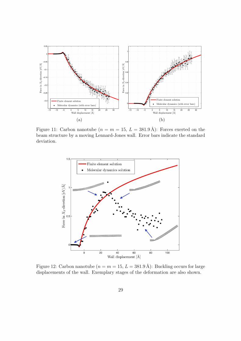
For the four systems, we present the computed mass-related quantities in table4, and the corresponding parameters for the constitutive law in table 5. For theCNTs with n = m = 10, 15, 20, 25 we find the following axial Young’s moduli:E = 643 GPa, 543 GPa, 426 GPa and 377 GPa. These quantities agree with datareported in the literature [3, 93–95], where a range between 300 GPa and 1 TPa istypically found. The axial shear modulus can be found by dividing the torsionalstiffness GJ by the polar moment of area J = R4

csπ/2. We obtain values of G =578 GPa, 501 GPa, 405 GPa and 364 GPa, respectively, which is also consistentwith other simulations [96, 97].

We can also have another look at how the material behavior changes undervariations in the temperature. For the (20, 20) system, the values correspondingto T = 300 K, 450 K, 600 K and 750 K are shown in table 6. Additional materialparameters have also been identified for the case that a certain vacancy percentagepd is introduced. Results for the (15, 15) system with vacancies are listed in table 7.Like before in the SiNW setting, a monotonous decrease of all stiffnesses can beobserved.

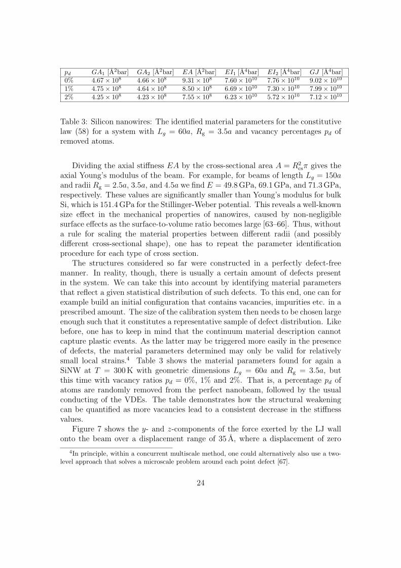
In figure 11, we see the y- and z-components of forces exerted on the (15, 15)CNT by the LJ wall as it is displaced 40.0 A. Again we observe good agreementbetween the atomistic and continuum mechanical surrogate models, including inthe attractive regime, but this suddenly changes if the wall is moved further: infigure 12, we see the carbon nanotube begin to buckle. This buckling cannotbe captured by our current finite element model. This phenomenon is also ac-companied by large deformations of the nanotube’s cross section, which are notaccounted for in the current formulation of the continuous beam. These structuralchanges in the cross section likely explain the apparent softening of the nanotube.Thus the atomistic modeling can be used to detect the range of applicability ofthe continuum model for a given system. Finally, in figure 13, we show the plot ofthe eccentricity of the CNT, which is also captured quite well.

5 Conclusion and Outlook

We have demonstrated how the procedure summarized in figure 1 can be used toobtain a surrogate model for atomistic beam structures. To this end, the theoryof geometrically exact beams [9] was chosen as a candidate for the description ofthe substituting continuum mechanical system. To assess the suitability of the

28

−15 −10 −5 0 5 10 15 20 25 30

−0.3

−0.25

−0.2

−0.15

−0.1

−0.05

0

0.05

Wall displacement [A]

Force

inX

2-direction

[eV/A

]

Finite element solution

Molecular dynamics (with error bars)

(a)

−15 −10 −5 0 5 10 15 20 25 30

0

0.2

0.4

0.6

0.8

1

Wall displacement [A]

Force

inX

3-direction

[eV/A

]

Finite element solution

Molecular dynamics (with error bars)

(b)

Figure 11: Carbon nanotube (n = m = 15, L = 381.9 A): Forces exerted on thebeam structure by a moving Lennard-Jones wall. Error bars indicate the standarddeviation.

Figure 12: Carbon nanotube (n = m = 15, L = 381.9 A): Buckling occurs for largedisplacements of the wall. Exemplary stages of the deformation are also shown.

29

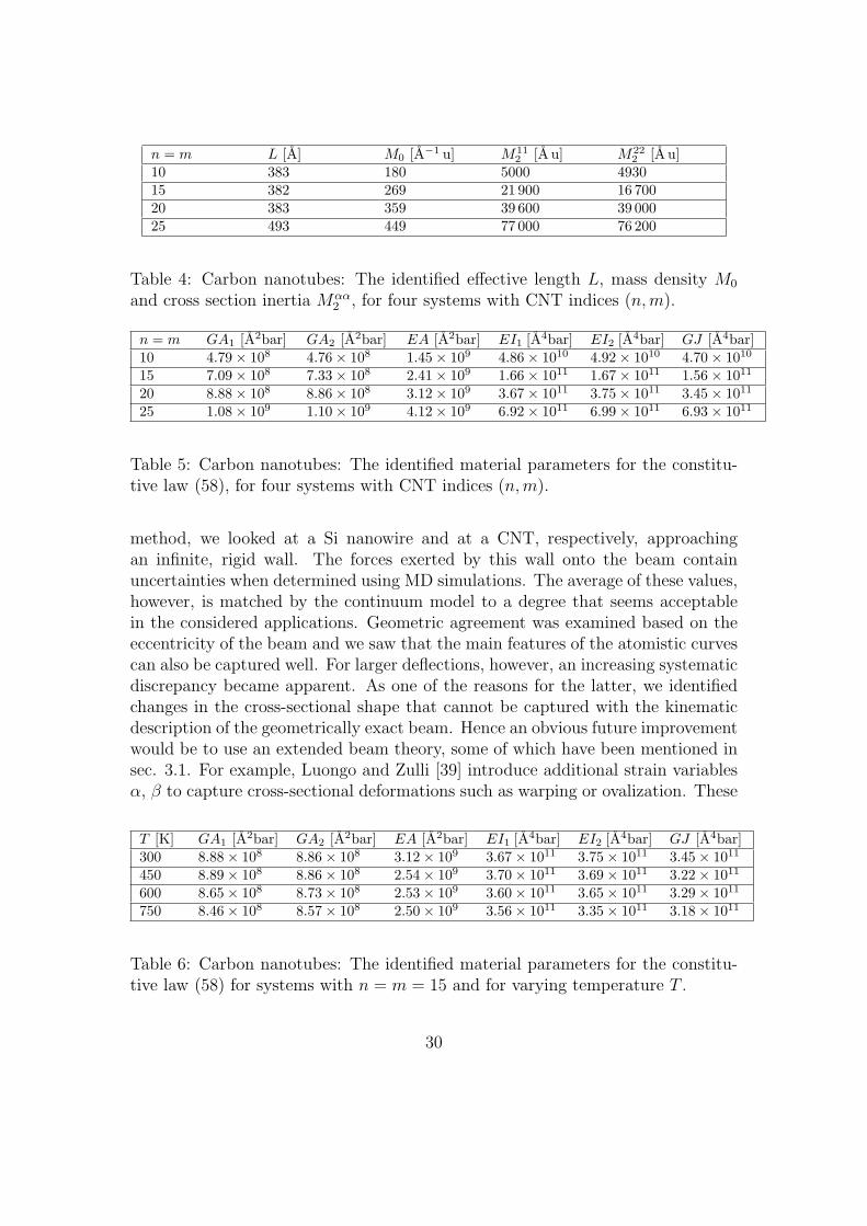
n = m L [A] M0 [A−1 u] M112 [A u] M22

2 [A u]10 383 180 5000 493015 382 269 21 900 16 70020 383 359 39 600 39 00025 493 449 77 000 76 200

Table 4: Carbon nanotubes: The identified effective length L, mass density M0

and cross section inertia Mαα2 , for four systems with CNT indices (n,m).

n = m GA1 [A2bar] GA2 [A2bar] EA [A2bar] EI1 [A4bar] EI2 [A4bar] GJ [A4bar]10 4.79× 108 4.76× 108 1.45× 109 4.86× 1010 4.92× 1010 4.70× 1010

15 7.09× 108 7.33× 108 2.41× 109 1.66× 1011 1.67× 1011 1.56× 1011

20 8.88× 108 8.86× 108 3.12× 109 3.67× 1011 3.75× 1011 3.45× 1011

25 1.08× 109 1.10× 109 4.12× 109 6.92× 1011 6.99× 1011 6.93× 1011

Table 5: Carbon nanotubes: The identified material parameters for the constitu-tive law (58), for four systems with CNT indices (n,m).

method, we looked at a Si nanowire and at a CNT, respectively, approachingan infinite, rigid wall. The forces exerted by this wall onto the beam containuncertainties when determined using MD simulations. The average of these values,however, is matched by the continuum model to a degree that seems acceptablein the considered applications. Geometric agreement was examined based on theeccentricity of the beam and we saw that the main features of the atomistic curvescan also be captured well. For larger deflections, however, an increasing systematicdiscrepancy became apparent. As one of the reasons for the latter, we identifiedchanges in the cross-sectional shape that cannot be captured with the kinematicdescription of the geometrically exact beam. Hence an obvious future improvementwould be to use an extended beam theory, some of which have been mentioned insec. 3.1. For example, Luongo and Zulli [39] introduce additional strain variablesα, β to capture cross-sectional deformations such as warping or ovalization. These

T [K] GA1 [A2bar] GA2 [A2bar] EA [A2bar] EI1 [A4bar] EI2 [A4bar] GJ [A4bar]300 8.88× 108 8.86× 108 3.12× 109 3.67× 1011 3.75× 1011 3.45× 1011

450 8.89× 108 8.86× 108 2.54× 109 3.70× 1011 3.69× 1011 3.22× 1011

600 8.65× 108 8.73× 108 2.53× 109 3.60× 1011 3.65× 1011 3.29× 1011

750 8.46× 108 8.57× 108 2.50× 109 3.56× 1011 3.35× 1011 3.18× 1011

Table 6: Carbon nanotubes: The identified material parameters for the constitu-tive law (58) for systems with n = m = 15 and for varying temperature T .

30

pd GA1 [A2bar] GA2 [A2bar] EA [A2bar] EI1 [A4bar] EI2 [A4bar] GJ [A4bar]0% 7.09× 108 7.33× 108 2.41× 109 1.66× 1011 1.67× 1011 1.56× 1011

1% 6.03× 108 5.87× 108 1.82× 109 1.58× 1011 1.59× 1011 1.40× 1011

2% 5.55× 108 5.27× 108 1.76× 109 1.42× 1011 1.44× 1011 1.25× 1011

Table 7: Carbon nanotubes: The identified material parameters for the constitu-tive law (58) for systems with n = m = 15 and vacancy percentages pd of removedatoms.

5 10 15 20 25 30 35 40 0

10

20

30

40

50

60

70

Wall displacement [A]

Eccentricity[A

]

Finite element solution

Molecular dynamics solution

Figure 13: Carbon nanotube (n = m = 15, L = 381.9 A): Eccentricity of thestructure at certain wall displacement levels.

31

satisfy an additional balance equation, typically of the form B′−D+ q = 0, whereq is a distortional force and D = ∂αψ and B = ∂βψ are the new stresses associatedwith the distortion. To fit the energy density ψ, the general method described inthis work would have to be supplemented by appropriate expressions that relatethe atomistic degrees of freedom q,p to the macroscopic quantities α, β, D andB based on phase averages.

Another plausible source of the mismatch could be that the linear constitutivelaw used does not describe the system well over the whole range of deformations.More complex functional forms might therefore be considered [18], or one couldadapt an arbitrary three-dimensional constitutive law to the reduced one-dimen-sional case. In any case, possible rate effects leading to non-relaxed stresses in theVDE at calibration should be avoided by granting sufficiently long equilibrationtimes. The material laws determined in this work could also be applied to adhesionand debonding problems involving thin films [98]. A potential future extension ofthe present work is posed by coupling the mechanical conservation laws to thegeneral energy balance:

P : F + ρ0r0 −DivH = ρ0e0, (81)

with referential heat source distribution r0, heat flux vector H and internal energydensity e0. One can then assume, for example, that the latter two quantitiesdepend on instantaneous strain and temperature,

H = H(Γ,Ω, T ), e0 = e0(Γ,Ω, T ). (82)

In the simplest case, the internal energy is a linear function of temperature:e0 = e0(T ) = cvT + const, where cv is the specific heat capacity. It was al-ready shown how the Helmholtz free energy can be determined in a temperature-dependent fashion, ψ = ψ(Γ,Ω, T ). However, a new procedure would have to beconceived to obtain suitable continuum mechanical constitutive laws for H ande0 from atomistic simulations. Numerous studies have attempted to address thisproblem for three-dimensional bulk systems Fish et al. [27], Admal and Tadmor[28], Lehoucq and Von Lilienfeld [99], Hardy [100], Wagner et al. [101]. One shouldkeep in mind, though, that capturing electron-based heat transfer requires suitablemodification of classical MD [102].

On the other hand, the computational costs of the FE simulations are much lesscompared to the fully atomistic ones. For example, the MD simulation of the beam-wall contact for carbon nanotube (n = m = 15) consisting of N = 8580 particlestakes about 100 h when running on 64 cores in parallel, due to the relativelylong simulation time of 98 ns. Compared with this, solving a series of 500 quasi-static continuum problems using 200 finite elements can be done on a conventional

32

workstation computer in just about one hour, though the one-time calibrationphase is not included in this.

We would thus expect large savings in computation time for more complexsystems. Some interesting candidates for the near future could for example includemulti-walled carbon nanotubes (MWCNT) or larger organic materials like bundlesof cellulose strands.

Acknowledgements

The authors are grateful to the German Research Foundation (DFG) for support-ing this research under projects GSC 111 and SA1822/5-1.

A Appendix: Analytical expressions for homo-

geneously deformed beams

To evaluate the integral expression in (27),

r(S) = rin + Λin

ñ∫ S

s=0expÄs · “Ω0

äds

ô· (Γ0 +E3). (83)

we first write Ω0 in terms of its polar angle θ and azimuth angle ψ:

Ω0 = ‖Ω0‖ ·

sin θ cosψsin θ sinψ

cos θ

. (84)

We then consider the diagonalization “Ω0 = V ·D · V ∗ with

D = diagÄi‖Ω0‖,−i‖Ω0‖, 0

ä, V =

îa+ ib,a− ib,Ω0/‖Ω0‖

ó, (85)

where we introduce

a =1√2

− cos θ cosψ− cos θ sinψ

sin θ

, b =1√2

− sinψcosψ

0

, (86)

and V ∗ is the complex conjugate of V . From this we obtain∫ S

s=0expÄs · “Ω0

äds = V ·

ñ∫ S

s=0exp(s ·D) ds

ô· V ∗ (87)

= V · diag

Çexp(iS‖Ω0‖)− 1

i‖Ω0‖,1− exp(iS‖Ω0‖)

i‖Ω0‖, S

å· V ∗,

(88)

33

which can be used to obtain the central line r(S) with respect to basis vectorsei for any homogeneous strain pair (Γ0,Ω0), as is apparent from (83). We are inparticular interested in the following resulting configurations for pure strains, withrin = 0, Λin = I chosen at the beam end S = 0.

1. Shear in x-direction, Γ0 = [Γ1, 0, 0], Ω0 = [0, 0, 0]:

r(S) =

Γ1

01

· S, Λ(S) ≡ I (89)

2. Shear in y-direction, Γ0 = [0,Γ2, 0], Ω0 = [0, 0, 0]:

r(S) =

0Γ2

1

· S, Λ(S) ≡ I (90)

3. Axial elongation or shortening, Γ0 = [0, 0,Γ3], Ω0 = [0, 0, 0]:

r(S) =

00

Γ3 + 1

· S, Λ(S) ≡ I (91)

4. Bending about x-axis, Γ0 = [0, 0, 0], Ω0 = [Ω1, 0, 0]:

r(S) =

01

Ω1(cos(S · Ω1)− 1)

1Ω1

sin(S · Ω1)

, Λ(S) =

1 0 00 cos(S · Ω1) − sin(S · Ω1)0 sin(S · Ω1) cos(S · Ω1)

(92)

5. Bending about y-axis, Γ0 = [0, 0, 0], Ω0 = [0,Ω2, 0]:

r(S) =

1

Ω2(cos(S · Ω2)− 1)

01

Ω2sin(S · Ω2)

, Λ(S) =

cos(S · Ω2) 0 sin(S · Ω2)0 1 0

− sin(S · Ω2) 0 cos(S · Ω2)

(93)

6. Axial torsion, Γ0 = [0, 0, 0], Ω0 = [0, 0,Ω3]:

r(S) =

00S

, Λ(S) =

cos(S · Ω3) − sin(S · Ω3) 0sin(S · Ω3) cos(S · Ω3) 0

0 0 1

(94)

34

B Appendix: Analytical expressions for Lennard-

Jones interactions of a beam

Suppose that for some mapping f : R3 → R we want to determine the integral∫Cf(r + ζαdα) dζ (95)

over the disk C = ζ ∈ R2 | ‖ζ‖ ≤ Rcs, for fixed values of r, dα. We can rewritethis as ∫

CfÄr + ζαdα

ädζ, dα := Qdα, (96)

for any proper orthogonal transformation Q that leaves d3 = Qd3 unchanged.This can be seen by considering the area-preserving transformation

T : C → C, ζα = TαÄζä

= ζβ dα ·Qdβ. (97)

If now f is substituted by dE(·)−3, where dE(y) = y · ν − d is the distance to theplane E from sec. 4.1, we can write

J3 :=∫CdE(r + ζαdα)−3 dζ =

∫CdEÄr + ζαdα

ä−3dζ. (98)

If we choose Q such that in addition it holds d2 · ν = Qd2 · ν = 0 we have

dEÄr + ζαdα

ä= r · ν − d︸ ︷︷ ︸

=:a=dE(r)

+ζ1 Qd1 · ν︸ ︷︷ ︸=:b

= a+ ζ1b. (99)

Based on this, and introducing l(t) :=»R2

cs − t2, the integral (98) over C becomes

∫C

Äa+ ζ1b

ä−3dζ =

Rcs∫ζ1=−Rcs

l(ζ1)∫ζ2=−l(ζ1)

Äa+ ζ1b

ä−3dζ1dζ2 (100)

=

Rcs∫ζ1=−Rcs

Äa+ ζ1b

ä−3 · 2lÄζ1ädζ1 (101)

=R2

cs π

(a−Rcs b)32 (a+Rcs b)

32

= J3(a, b, Rcs). (102)

In the context of the Lennard-Jones wall interaction, we can note that dEÄr + ζαdα

ä>

0 for all ζ ∈ C since the beam remains in E+. Hence we have

0 < dEÄr + ζαdα

ä= dE

Är + ζ1d1

ä= a+ ζ1 b, ∀ζ =

Äζ1, ζ2

ä∈ C. (103)

35

If we insert the extremal values ζ1 = ±Rcs this yields the inequalities a+Rcs b > 0and a− Rcs b > 0. This shows that no singularities appear in the denominator ofJ3(a, b, R).

One possibility (of two) for a rotation Q that satisfies the aforementionedconditions is given explicitly by

Q =

ñ1

sin γ(d3 × ν)× d3

ô⊗ d1 +

ñ1

sin γd3 × ν

ô⊗ d2 + d3 ⊗ d3, (104)

with γ denoting the angle between d3 and ν. It then becomes obvious that b =Qd1 · ν = sin γ. And as we already know that a = dE(r) is the distance of thedisk center to the wall, we see that

J3 = J3(a, b, Rcs) = J3(dE(r), sin γ,Rcs) (105)

is really just a function of the disk center’s distance, the angle between disk andwall normals and the disk radius. Lastly, analogously to J3, we can also obtain

J9(a, b, Rcs) :=∫CdE(r + ζαdα)−9 dζ =

R2cs π

64·5b

6R6cs + 120a2b4R4

cs + 240a4b2R2cs + 64a6

(a−Rcs b)15/2(a+Rcs b)

15/2.

(106)

References

[1] Charles M Lieber and Zhong Lin Wang. Functional nanowires. MRS Bulletin,32(02):99–108, 2007.

[2] D. Qian, G. J. Wagner, and W. K. Liu. A multiscale projection methodfor the analysis of carbon nanotubes. Comput. Methods Appl. Mech. Engrg.,193:1603–1632, 2004.

[3] Rodney S Ruoff, Dong Qian, and Wing Kam Liu. Mechanical properties ofcarbon nanotubes: theoretical predictions and experimental measurements.Comptes Rendus Physique, 4(9):993–1008, 2003.

[4] Brooks D. Rabideau, Animesh Agarwal, and Ahmed E. Ismail. Observedmechanism for the breakup of small bundles of cellulose Iα and Iβ inionic liquids from molecular dynamics simulations. The Journal of Phys-ical Chemistry B, 117(13):3469–3479, 2013. doi: 10.1021/jp310225t. URLhttp://pubs.acs.org/doi/abs/10.1021/jp310225t.

[5] Christian J Cyron and Wolfgang A Wall. Consistent finite-element approachto Brownian polymer dynamics with anisotropic friction. Physical review.E, Statistical, nonlinear, and soft matter physics, 82(6 Pt 2):066705–066705,2010.

36

[6] Christian J Cyron, Kei W Muller, Andreas R Bausch, and Wolfgang A Wall.Micromechanical simulations of biopolymer networks with finite elements.Journal of Computational Physics, 244:236–251, 2013.

[7] I Romero, M Urrecha, and CJ Cyron. A torsion-free non-linear beam model.International Journal of Non-Linear Mechanics, 58:1–10, 2014.

[8] M Fixman and J Kovac. Polymer conformational statistics. III. ModifiedGaussian models of stiff chains. The Journal of Chemical Physics, 58:1564,1973.

[9] JC Simo. A finite strain beam formulation. The three-dimensional dynamicproblem. Part I. Computer methods in applied mechanics and engineering,49(1):55–70, 1984.

[10] Stuart S Antman. Nonlinear problems of elasticity, volume 107. Springer,2005.

[11] Ryan S Elliott, Nicolas Triantafyllidis, and John A Shaw. Stability of crys-talline solids — I: Continuum and atomic lattice considerations. Journal ofthe Mechanics and Physics of Solids, 54(1):161–192, 2006.

[12] M Arroyo and T Belytschko. Finite element methods for the non-linearmechanics of crystalline sheets and nanotubes. International Journal forNumerical Methods in Engineering, 59(3):419–456, 2004.

[13] Jerry Z Yang and Weinan E. Generalized Cauchy-Born rules for elasticdeformation of sheets, plates, and rods: Derivation of continuum modelsfrom atomistic models. Physical Review B, 74(18):184110, 2006.

[14] Ye Hakobyan, EB Tadmor, and RD James. Objective quasicontinuum ap-proach for rod problems. Physical Review B, 86(24):245435, 2012.

[15] Gero Friesecke and Richard D James. A scheme for the passage from atomicto continuum theory for thin films, nanotubes and nanorods. Journal of theMechanics and Physics of Solids, 48(6):1519–1540, 2000.

[16] Bernd Schmidt. On the passage from atomic to continuum theory for thinfilms. Archive for rational mechanics and analysis, 190(1):1–55, 2008.

[17] Karthick Chandraseker, Subrata Mukherjee, Jeffrey T Paci, and George CSchatz. An atomistic-continuum cosserat rod model of carbon nanotubes.Journal of the Mechanics and Physics of Solids, 57(6):932–958, 2009.

37

[18] Chao Fang, Ajeet Kumar, and Subrata Mukherjee. Finite element analysisof single-walled carbon nanotubes based on a rod model including in-planecross-sectional deformation. International Journal of Solids and Structures,50(1):49–56, 2013.

[19] Youping Chen and James D Lee. Connecting molecular dynamics to mi-cromorphic theory. (I). Instantaneous and averaged mechanical variables.Physica A: Statistical Mechanics and its Applications, 322:359–376, 2003.

[20] Youping Chen and James D Lee. Connecting molecular dynamics to micro-morphic theory. (II). Balance laws. Physica A: Statistical Mechanics and itsApplications, 322:377–392, 2003.

[21] Ellad B. Tadmor and Ronald E. Miller. Modeling Materials: Continuum,Atomistic and Multiscale Techniques. Cambridge University Press, 2011.

[22] H Jiang, Y Huang, and KC Hwang. A finite-temperature continuum the-ory based on interatomic potentials. Journal of engineering materials andtechnology, 127(4):408–416, 2005.

[23] SJV Frankland, VM Harik, GM Odegard, DW Brenner, and TS Gates. Thestress–strain behavior of polymer–nanotube composites from molecular dy-namics simulation. Composites Science and Technology, 63(11):1655–1661,2003.

[24] P. T. Bauman, J. T. Oden, and S. Prudhomme. Adaptive multiscale model-ing of polymeric materials: Arlequin coupling and goals algorithms. Comput.Methods Appl. Mech. Engrg., 198:799–818, 2009.

[25] Marcus G Schmidt, Roger A Sauer, and Ahmed E Ismail. Multiscale treat-ment of mechanical contact problems involving thin polymeric layers. Mod-elling and Simulation in Materials Science and Engineering, 22(4):045012,2014.

[26] Wen Chen and Jacob Fish. A generalized space–time mathematical homog-enization theory for bridging atomistic and continuum scales. InternationalJournal for Numerical Methods in Engineering, 67(2):253–271, 2006.

[27] Jacob Fish, Wen Chen, and Renge Li. Generalized mathematical homoge-nization of atomistic media at finite temperatures in three dimensions. Com-puter methods in applied mechanics and engineering, 196(4):908–922, 2007.

[28] Nikhil Chandra Admal and EB Tadmor. Stress and heat flux for arbitrarymultibody potentials: A unified framework. The Journal of chemical physics,134:184106, 2011.

38

[29] D Davydov and P Steinmann. Reviewing the roots of continuum formula-tions in molecular systems. part iii: Stresses, couple stresses, heat fluxes.Mathematics and Mechanics of Solids, page 1081286513516480, 2013.

[30] DA McQuarrie. Statistical Mechanics. University Science, Sausalito, USA,2000.

[31] Nikhil Chandra Admal and Ellad B Tadmor. A unified interpretation ofstress in molecular systems. Journal of Elasticity, 100(1-2):63–143, 2010.

[32] Stuart S Antman. The theory of rods. In Linear Theories of Elasticity andThermoelasticity, pages 641–703. Springer, 1973.

[33] I Romero and F Armero. An objective finite element approximation of thekinematics of geometrically exact rods and its use in the formulation of anenergy–momentum conserving scheme in dynamics. International Journalfor Numerical Methods in Engineering, 54(12):1683–1716, 2002.

[34] Juan C Simo and Loc Vu-Quoc. A geometrically-exact rod model incor-porating shear and torsion-warping deformation. International Journal ofSolids and Structures, 27(3):371–393, 1991.

[35] N Silvestre and D Camotim. Nonlinear generalized beam theory for cold-formed steel members. International Journal of Structural Stability and Dy-namics, 3(04):461–490, 2003.

[36] Marcello Pignataro, Nicola Rizzi, Giuseppe Ruta, and Valerio Varano. Theeffects of warping constraints on the buckling of thin-walled structures. Jour-nal of Mechanics of Materials and Structures, 4(10):1711–1727, 2010.

[37] Ajeet Kumar and Subrata Mukherjee. A geometrically exact rod model in-cluding in-plane cross-sectional deformation. Journal of Applied Mechanics,78(1):011010, 2011.

[38] P Lidstrom. On the equations of motion for curved slender beams us-ing tubular coordinates. Mathematics and Mechanics of Solids, page1081286513487188, 2013.

[39] A Luongo and D Zulli. A non-linear one-dimensional model of cross-deformable tubular beam. International Journal of Non-Linear Mechanics,2014.

[40] JC Simo and Loc Vu-Quoc. A three-dimensional finite-strain rod model.part ii: Computational aspects. Computer methods in applied mechanicsand engineering, 58(1):79–116, 1986.

39

[41] Juan Carlos Simo and Loc Vu-Quoc. On the dynamics in space of rods un-dergoing large motions—a geometrically exact approach. Computer methodsin applied mechanics and engineering, 66(2):125–161, 1988.

[42] G Jelenic and MA Crisfield. Geometrically exact 3D beam theory: Im-plementation of a strain-invariant finite element for statics and dynamics.Computer Methods in Applied Mechanics and Engineering, 171(1):141–171,1999.

[43] S Leyendecker, P Betsch, and P Steinmann. Objective energy–momentumconserving integration for the constrained dynamics of geometrically exactbeams. Computer Methods in Applied Mechanics and Engineering, 195(19):2313–2333, 2006.

[44] Francois Demoures, Francois Gay-Balmaz, Thomas Leitz, Sigrid Leyen-decker, Sina Ober-Blobaum, and Tudor S Ratiu. Asynchronous variationallie group integration for geometrically exact beam dynamics. PAMM, 13(1):45–46, 2013.

[45] SR Eugster, C Hesch, P Betsch, and Ch Glocker. Director-based beam finiteelements relying on the geometrically exact beam theory formulated in skewcoordinates. International Journal for Numerical Methods in Engineering,97(2):111–129, 2014.

[46] Ignacio Romero. The interpolation of rotations and its application to finiteelement models of geometrically exact rods. Computational mechanics, 34(2):121–133, 2004.

[47] FA McRobie and J Lasenby. Simo–Vu Quoc rods using Clifford algebra.International Journal for Numerical Methods in Engineering, 45(4):377–398,1999.

[48] Eva Zupan, Miran Saje, and Dejan Zupan. The quaternion-based three-dimensional beam theory. Computer methods in applied mechanics and en-gineering, 198(49):3944–3956, 2009.

[49] Hongzhi Zhong, Run Zhang, and Naijia Xiao. A quaternion-based weakform quadrature element formulation for spatial geometrically exact beams.Archive of Applied Mechanics, pages 1–16, 2014.

[50] E Celledoni and N Safstrom. A Hamiltonian and multi-Hamiltonian for-mulation of a rod model using quaternions. Computer Methods in AppliedMechanics and Engineering, 199(45):2813–2819, 2010.

40

[51] MATLAB. Version 7.11.0 (R2011a). The MathWorks Inc., Natick, Mas-sachusetts, 2011.

[52] M. F. Horstemeyer and M. I. Baskes. Strain tensors at the atomic scale.MRS Proceedings, 578, 1 1999. ISSN null. doi: 10.1557/PROC-578-15. URLhttp://journals.cambridge.org/article_S1946427400297832.

[53] Jonathan A. Zimmerman, Douglas J. Bammann, and Huajian Gao. De-formation gradients for continuum mechanical analysis of atomistic simu-lations. International Journal of Solids and Structures, 46(2):238 – 253,2009. ISSN 0020-7683. doi: 10.1016/j.ijsolstr.2008.08.036. URL http:

//www.sciencedirect.com/science/article/pii/S002076830800348X.

[54] Jonathan A Zimmerman, Reese E Jones, and Jeremy A Templeton. A ma-terial frame approach for evaluating continuum variables in atomistic simu-lations. Journal of Computational Physics, 229(6):2364–2389, 2010.

[55] John R Ray and Aneesur Rahman. Statistical ensembles and moleculardynamics studies of anisotropic solids. The Journal of chemical physics, 80:4423, 1984.

[56] Steve Plimpton. Fast parallel algorithms for short-range molecular dynamics.Journal of Computational Physics, 117(1):1 – 19, 1995. ISSN 0021-9991. doi:10.1006/jcph.1995.1039. URL http://lammps.sandia.gov.

[57] B. S. Kirk, J. W. Peterson, R. H. Stogner, and G. F. Carey. libMesh: AC++ library for parallel adaptive mesh refinement/coarsening simulations.Engineering with Computers, 22(3–4):237–254, 2006.

[58] Roger A. Sauer and Peter Wriggers. Formulation and analysis of athree-dimensional finite element implementation for adhesive contact atthe nanoscale. Computer Methods in Applied Mechanics and Engineer-ing, 198(49–52):3871 – 3883, 2009. ISSN 0045-7825. doi: 10.1016/j.cma.2009.08.019. URL http://www.sciencedirect.com/science/article/

pii/S0045782509002631.

[59] Frank H. Stillinger and Thomas A. Weber. Computer simulation of localorder in condensed phases of silicon. Physical Review B, 31:5262–5271, 1985.

[60] Jijun Lao, Mehdi Naghdi Tam, Dinesh Pinisetty, and Nikhil Gupta. Molec-ular dynamics simulation of fcc metallic nanowires: A review. JOM, 65(2):175–184, 2013.

41

[61] Yong Zhu, Feng Xu, Qingquan Qin, Wayne Y Fung, and Wei Lu. Mechanicalproperties of vapor–liquid–solid synthesized silicon nanowires. Nano letters,9(11):3934–3939, 2009.

[62] Dai-Ming Tang, Cui-Lan Ren, Ming-Sheng Wang, Xianlong Wei, NaoyukiKawamoto, Chang Liu, Yoshio Bando, Masanori Mitome, Naoki Fukata, andDmitri Golberg. Mechanical properties of Si nanowires as revealed by in situtransmission electron microscopy and molecular dynamics simulations. Nanoletters, 12(4):1898–1904, 2012.

[63] Ronald E Miller and Vijay B Shenoy. Size-dependent elastic properties ofnanosized structural elements. Nanotechnology, 11(3):139, 2000.

[64] CQ Chen, Y Shi, YS Zhang, J Zhu, and YJ Yan. Size dependence of Young’smodulus in ZnO nanowires. Physical Review Letters, 96(7):075505, 2006.

[65] Byeongchan Lee and Robert E Rudd. First-principles study of the Young’smodulus of Si¡001¿ nanowires. Physical review B, 75(4):041305, 2007.

[66] Keonwook Kang and Wei Cai. Size and temperature effects on the fracturemechanisms of silicon nanowires: Molecular dynamics simulations. Interna-tional Journal of Plasticity, 26(9):1387–1401, 2010.

[67] Arif Masud and Raguraman Kannan. A multiscale framework for compu-tational nanomechanics: Application to the modeling of carbon nanotubes.International journal for numerical methods in engineering, 78(7):863–882,2009.

[68] A Krishnan, E Dujardin, TW Ebbesen, PN Yianilos, and MMJ Treacy.Young’s modulus of single-walled nanotubes. Physical Review B, 58(20):14013, 1998.

[69] Tobias Hertel, Robert E Walkup, and Phaedon Avouris. Deformation ofcarbon nanotubes by surface van der Waals forces. Physical Review B, 58(20):13870, 1998.

[70] Jamie H Warner, Neil P Young, Angus I Kirkland, and G Andrew D Briggs.Resolving strain in carbon nanotubes at the atomic level. Nature materials,10(12):958–962, 2011.

[71] Dong Qian, Gregory J Wagner, Wing Kam Liu, Min-Feng Yu, and Rodney SRuoff. Mechanics of carbon nanotubes. Applied mechanics reviews, 55(6):495–533, 2002.

42

[72] Sanjay Govindjee and Jerome L Sackman. On the use of continuum mechan-ics to estimate the properties of nanotubes. Solid State Communications, 110(4):227–230, 1999.

[73] NJ Glassmaker and CY Hui. Elastica solution for a nanotube formed by self-adhesion of a folded thin film. Journal of applied physics, 96(6):3429–3434,2004.

[74] H Ustunel, D Roundy, and TA Arias. Modeling a suspended nanotube os-cillator. Nano letters, 5(3):523–526, 2005.

[75] Xian-Long Wei, Yang Liu, Qing Chen, Ming-Sheng Wang, and Lian-MaoPeng. The very-low shear modulus of multi-walled carbon nanotubes de-termined simultaneously with the axial Young’s modulus via in situ experi-ments. Advanced Functional Materials, 18(10):1555–1562, 2008.

[76] KM Liew, CH Wong, XQ He, MJ Tan, and SA Meguid. Nanomechanics ofsingle and multiwalled carbon nanotubes. Physical review B, 69(11):115429,2004.

[77] XQ He, S Kitipornchai, and KM Liew. Buckling analysis of multi-walledcarbon nanotubes: a continuum model accounting for van der Waals in-teraction. Journal of the Mechanics and Physics of Solids, 53(2):303–326,2005.

[78] Ning Liu, Yong-Gang Wang, Min Li, and Jiao Jia. Nonlinear buckling anal-yses of a small-radius carbon nanotube. Journal of Applied Physics, 115(15):154301, 2014.

[79] YY Zhang, CM Wang, WH Duan, Yang Xiang, and Z Zong. Assessment ofcontinuum mechanics models in predicting buckling strains of single-walledcarbon nanotubes. Nanotechnology, 20(39):395707, 2009.

[80] Tim Gould and David A Burton. A Cosserat rod model with microstructure.New Journal of Physics, 8(8):137, 2006.

[81] P Zhang, Y Huang, H Gao, and KC Hwang. Fracture nucleation in single-wall carbon nanotubes under tension: a continuum analysis incorporatinginteratomic potentials. Journal of Applied Mechanics, 69(4):454–458, 2002.

[82] SK Georgantzinos and NK Anifantis. Vibration analysis of multi-walledcarbon nanotubes using a spring–mass based finite element model. Compu-tational Materials Science, 47(1):168–177, 2009.

43

[83] Tienchong Chang. A molecular based anisotropic shell model for single-walled carbon nanotubes. Journal of the Mechanics and Physics of Solids,58(9):1422–1433, 2010.

[84] Yu Zhang, Carlo Sansour, Chris Bingham, et al. Single-walled carbon nan-otube modelling based on cosserat surface theory. Recent Advances in Elec-trical and Computer Engineering, pages 32–37, 2013.

[85] Sulin Zhang, Steven L Mielke, Roopam Khare, Diego Troya, Rodney S Ruoff,George C Schatz, and Ted Belytschko. Mechanics of defects in carbon nan-otubes: atomistic and multiscale simulations. Physical Review B, 71(11):115403, 2005.

[86] Stefan Hollerer. Numerical validation of a concurrent atomistic-continuummultiscale method and its application to the buckling analysis of carbonnanotubes. Computer Methods in Applied Mechanics and Engineering, 270:220–246, 2014.

[87] J. Tersoff. Modeling solid-state chemistry: Interatomic potentials for multi-component systems. Phys. Rev. B, 39:5566–5568, Mar 1989. doi: 10.1103/PhysRevB.39.5566. URL http://link.aps.org/doi/10.1103/PhysRevB.

39.5566.

[88] LA Girifalco, Miroslav Hodak, and Roland S Lee. Carbon nanotubes, buck-yballs, ropes, and a universal graphitic potential. Physical Review B, 62(19):13104, 2000.

[89] R Ansari, F Sadeghi, and S Ajori. Continuum and molecular dynamics studyof C60 fullerene–carbon nanotube oscillators. Mechanics Research Commu-nications, 47:18–23, 2013.

[90] William Humphrey, Andrew Dalke, and Klaus Schulten. VMD: Visual Molec-ular Dynamics. Journal of Molecular Graphics, 14:33–38, 1996.

[91] Marc Robinson and NA Marks. Nanocap: A framework for generatingcapped carbon nanotubes and fullerenes. Computer Physics Communica-tions, 2014.

[92] Ali Ghavamian, Moones Rahmandoust, and Andreas Ochsner. On the de-termination of the shear modulus of carbon nanotubes. Composites Part B:Engineering, 44(1):52–59, 2013.

[93] Jian Ping Lu. Elastic properties of carbon nanotubes and nanoropes. Phys-ical Review Letters, 79(7):1297, 1997.

44

[94] Jean-Paul Salvetat, G Andrew D Briggs, Jean-Marc Bonard, Revathi RBacsa, Andrzej J Kulik, Thomas Stockli, Nancy A Burnham, and LaszloForro. Elastic and shear moduli of single-walled carbon nanotube ropes.Physical Review Letters, 82(5):944, 1999.

[95] Michael Griebel and Jan Hamaekers. Molecular dynamics simulations of theelastic moduli of polymer–carbon nanotube composites. Computer Methodsin Applied Mechanics and Engineering, 193(17):1773–1788, 2004.

[96] Byeong-Woo Jeong, Jang-Keun Lim, and Susan B Sinnott. Elastic torsionalresponses of carbon nanotube systems. Journal of applied physics, 101(8):084309, 2007.

[97] AR Khoei, E Ban, P Banihashemi, and MJ Abdolhosseini Qomi. Effects oftemperature and torsion speed on torsional properties of single-walled carbonnanotubes. Materials Science and Engineering: C, 31(2):452–457, 2011.

[98] Roger A Sauer and Janine C Mergel. A geometrically exact finite beamelement formulation for thin film adhesion and debonding. Finite Elementsin Analysis and Design, 86:120–135, 2014.

[99] Richard B Lehoucq and Anatole Von Lilienfeld. Translation of walter noll’s“derivation of the fundamental equations of continuum thermodynamicsfrom statistical mechanics”. Journal of Elasticity, 100(1-2):5–24, 2010.

[100] Robert J Hardy. Formulas for determining local properties in molecular-dynamics simulations: Shock waves. The Journal of Chemical Physics, 76(1):622–628, 1982.

[101] Gregory J Wagner, RE Jones, JA Templeton, and ML Parks. An atomistic-to-continuum coupling method for heat transfer in solids. Computer Methodsin Applied Mechanics and Engineering, 197(41):3351–3365, 2008.

[102] DM Duffy and AM Rutherford. Including the effects of electronic stoppingand electron–ion interactions in radiation damage simulations. Journal ofPhysics: Condensed Matter, 19(1):016207, 2007.

45