a constraint in teaching mathematics - geometry …geometryexpressions.com/downloads/lessons/using a...

Professional Development Unit for

Using a Constraint Approach in Teaching Mathematics

Professional Development Unit for Geometry Expressions

Using a Constraint Approach in Teaching Mathematics

Jim Wiechmann Tualatin High School, Tualatin, OR, USA

Tim Brown

Naches Valley High School Naches, WA, USA

Saltire Software, Inc., Beaverton, OR USA

www.geometryexpressions.com

www.saltire.com

Table of Contents

Introduction 4

Guide to the Screen 5

Lesson 1: Using the Constraint Approach 6

Lesson 2: Drawing Geometric Figures 11

Lesson 3: Symbolic Outputs and Real Outputs 17

Lesson 4: Variation and Animation 20

Lesson 5: Functions and Loci 22

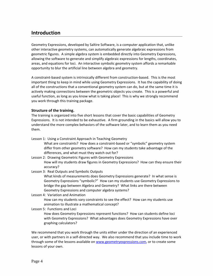
Introduction Geometry Expressions, developed by Saltire Software, is a computer application that, unlike other interactive geometry systems, can automatically generate algebraic expressions from geometric figures. A simple algebra system is embedded directly into Geometry Expressions, allowing the software to generate and simplify algebraic expressions for lengths, coordinates, areas, and equations for loci. An interactive symbolic geometry system affords a remarkable opportunity to blur the artificial line between algebra and geometry. A constraint‐based system is intrinsically different from construction‐based. This is the most important thing to keep in mind while using Geometry Expressions. It has the capability of doing all of the constructions that a conventional geometry system can do, but at the same time it is actively making connections between the geometric objects you create. This is a powerful and useful function, as long as you know what is taking place! This is why we strongly recommend you work through this training package. Structure of the training. The training is organized into five short lessons that cover the basic capabilities of Geometry Expressions. It is not intended to be exhaustive. A firm grounding in the basics will allow you to understand the more complex behaviors of the software later, and to learn them as you need them. Lesson 1: Using a Constraint Approach in Teaching Geometry

What are constraints? How does a constraint‐based or “symbolic” geometry system differ from other geometry software? How can my students take advantage of the differences, and what must they watch out for?

Lesson 2: Drawing Geometric Figures with Geometry Expressions How will my students draw figures in Geometry Expressions? How can they ensure their accuracy?

Lesson 3: Real Outputs and Symbolic Outputs What kinds of measurements does Geometry Expressions generate? In what sense is Geometry Expressions “symbolic?” How can my students use Geometry Expressions to bridge the gap between Algebra and Geometry? What links are there between Geometry Expressions and computer algebra systems?

Lesson 4: Variation and Animation How can my students vary constraints to see the effect? How can my students use animation to illustrate a mathematical concept?

Lesson 5: Functions and Loci How does Geometry Expressions represent functions? How can students define loci with Geometry Expressions? What advantages does Geometry Expressions have over graphing calculators?

We recommend that you work through the units either under the direction of an experienced user, or with partners in a self‐directed way. We also recommend that you include time to work through some of the lessons available on www.geometryexpressions.com, or to create some lessons of your own.

http://www.geometryexpressions.com/

Guide to the Screen Here is a map of the Geometry Expressions Window. You’ll learn its functions in context as you move through the training lessons.

These are tool panels. Almost all of the functions in Geometry Expressions are accessible through the tool panels. You can add and remove tool panels by selecting View on the Main menu.

The main menu and the icon bar are located at the top of the page

The status line tells you what you are doing, the coordinates of your pointer, and whether you are in degrees or radians.

Create your geometrical objects in this large drawing area.

When you are asked to click on an icon in a tool panel, the name of the panel and the icon are written in bold, and a picture of the icon will often be included. For example:

Click on constrain radius . If you “hover” the pointer over an icon, the name of the icon is displayed. Menu selections are often written with slashes, in this format:

Edit/Preferences/Geometry/Line Color

Or as step‐by‐step instructions. Select Edit from the menu bar. Choose Preferences. Click on Geometry and change the Line Color to blue.

Lesson 1: Using the Constraint Approach The intent of each Professional Development lesson is to explore how Geometry Expressions can be used to enhance classroom learning. Each unit addresses a particular feature of Geometry Expressions that may be different from other dynamic geometry tools that you have used. This lesson explores the concept of a constraint system. A constraint system allows you to define geometrical objects in terms of other geometrical objects. Some of the constraints that you may impose on a geometrical object are A fixed length A fixed angle measure (including perpendicularity) A fixed direction or slope A fixed position Tangency Incidence Algebraic equation These constraints are fixed in that they define other geometrical objects. You, the software user, can easily change them. The result is that the other geometrical objects are changed as well. Keep in mind that mathematically, a good definition only includes characteristics that are necessary and sufficient. We generally have little trouble violating the “necessary” part of a definition – often we are still in the process of defining, or we wish to leave some parts undefined. I’m sure you’ve had this exchange in your classroom. “Draw a triangle.” “What kind of triangle?” “It doesn’t matter – any triangle will work.” The triangle created would be underconstrained.” Conversely, you could overconstrain the triangle, violating the “sufficient” part of the definition: “Draw an equilateral triangle with 60° angles.” “Don’t they have to be 60°?”

“Excellent! Remember, class, that the angles of an equilateral triangle are all 60°.” Geometry Expressions will not allow you to overconstrain a geometrical object. It will remind you that your definition is already sufficient, and that any more constraints may or may not lead to a contradiction. This lesson on Triangle Congruency Theorems is intended to exploit Geometry Expressions’ detection of redundant constraints.

Name: __________________________________ Date: __________________________________

Nailing Down Triangles

The definition of a triangle is easy: it’s a closed figure on a plane that is formed by three line segments. But how much information do you need to define a particular triangle – that is, one of a particular size and shape? Open Geometry Expressions and get started! First, make sure Geometry Expressions is in angle mode.

Select Edit from the menu bar. Choose Preferences. Click on the Math icon on the right side of the dialog box. Toggle Angle Mode to Degrees.

1. Draw a triangle with the segment tool or the polygon tool . Don’t forget to click

on the select tool when you are finished. Click and drag on parts of the triangle. You can see that you’ve created a triangle, but no triangle in particular. See if you can create the triangle in Diagram 1. Define the length of a side by selecting the side and

then using the constrain length tool. Define the measure of an angle by selecting both

sides of the angle and then using the constrain angle tool. You’ll be done before you know it! Did you finish drawing the triangle? How far did you get?

30°

60°

90°

510

5 3

Diagram 1

46° 62°

Diagram 2

2. The reason that you got stuck before you finished is that Geometry Expressions won’t let you tell it anything that it can figure out for itself. At first, this can be frustrating, but in fact it can be very powerful. Look at the triangle in Diagram 2. What is the measure of the third angle? Draw the triangle in Geometry Expressions. Can you constrain all three angles? What happens if you try?

Geometry Expressions won’t let you constrain the third angle, because it knows it can figure it out. It lets you know with dialog box in Diagram 3. If you want to find out what the measure of the third angle is, choose “Calculate the angle from other constraints.”

You can use Geometry Expressions to create a conjecture. Change the measures of your angles from 62° and 46° to x and y.

Diagram 3

If the measures of two angles in a triangle are x and y, then the measure of the third angle is _____________________________________________________________________

Try dragging your triangle around now. You’ll see that the angles change. That’s because dragging is like typing in different numbers for x or y. Select x in the

Variable Tool Panel, and click on the lock icon . That will keep the variable from changing when you drag. Do the same for y.

Drag the triangle around. Does your triangle keep its size and shape?

3. So far we’ve learned that you can only constrain two out of the three angles in a

triangle, but that’s not enough to nail down its size and shape.

Constrain sides until you get the dialog boxing complaining about your constrain. How many sides did you constrain before you got the dialog box? Which side or sides did you constrain – between the angles, or not between the angles?

Compare your results with those around you. Sum up your findings here:

4. Start over with a new triangle. This time we’re going to constrain sides instead of

angles. Start constraining the sides. You can use symbols or numbers, but if you violate the triangle inequality your triangle will disappear. At each step, lock the variable and see if the triangle stays the same shape and size. Compare your results with those around you, and sum up your findings: Can you constrain an angle once all your sides are constrained? If you get the dialog box, click on “Calculate the angle from other constraints.” Is it possible to find the measure of an angle in a triangle if you only know the lengths of the sides?

5. Continue your investigation with different combinations of angles and sides that you haven’t yet tried.

How many total constraints are necessary to define a triangle of particular shape and size?

Are there any combinations that are exceptions to the rule?

6. One of the combinations of sides and angles does require one more bit of

information to be complete: if you have two sides constrained, and the angle that is not between the sides is constrained. Draw the triangle in Diagram 4 using Geometry Expressions. Constrain the sides and angle shown.

θ

b a

Make sure this angle looks obtuse.

Diagram 4

Now, add a line segment as shown in Diagram 5. How many triangles are there with angle θ

θ

b a

Diagram 5

a and

sides of length a and b?

Geometry Expressions uses your drawing to decide which triangle you intend. 7. Summary

You need ____ of the measures of a triangle defined before you establish its size and shape.

__________ does not work, since you can always find one angle from the other two.

_______________ only works if you know __________________________________.

Extension:

Use Geometry Expressions to discover which combinations of sides and angles can be used to determine a quadrilateral’s size and shape.

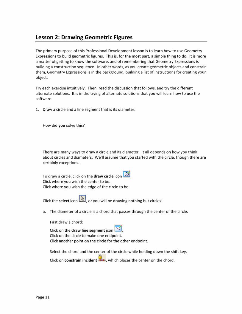
Lesson 2: Drawing Geometric Figures The primary purpose of this Professional Development lesson is to learn how to use Geometry Expressions to build geometric figures. This is, for the most part, a simple thing to do. It is more a matter of getting to know the software, and of remembering that Geometry Expressions is building a construction sequence. In other words, as you create geometric objects and constrain them, Geometry Expressions is in the background, building a list of instructions for creating your object. Try each exercise intuitively. Then, read the discussion that follows, and try the different alternate solutions. It is in the trying of alternate solutions that you will learn how to use the software. 1. Draw a circle and a line segment that is its diameter.

How did you solve this? There are many ways to draw a circle and its diameter. It all depends on how you think about circles and diameters. We’ll assume that you started with the circle, though there are certainly exceptions.

To draw a circle, click on the draw circle icon . Click where you wish the center to be. Click where you wish the edge of the circle to be.

Click the select icon , or you will be drawing nothing but circles!

a. The diameter of a circle is a chord that passes through the center of the circle.

First draw a chord:

Click on the draw line segment icon . Click on the circle to make one endpoint. Click another point on the circle for the other endpoint.

Select the chord and the center of the circle while holding down the shift key.

Click on constrain incident , which places the center on the chord.

b. Another way to draw a chord that passes through the center is to draw an infinite line through the center, and then find its points of intersection with the circle.

Click on the draw infinite line icon . Click on the center of the circle (it will “highlight” when your pointer is on the center.) Select the line and the circle while holding the shift key.

Click on the construct intersection icon .

c. The diameter of a circle is two radii that form an angle of 180° or π radians.

Use the draw line segment tool to draw to radii. Hold shift and select both segments.

Click on the constrain angle icon . There is an indicator in the lower right corner of the window that will tell you if you are in degree mode or radian mode. Type either 180 or click the π icon in the symbols tool panel.

d. The diameter of a circle is a chord with length twice the radius.

Select the circle and click on constrain radius . Leave the length of the radius as r. Draw a chord.

Select the chord and click on constrain distance . Type 2*r. Geometry Expressions allows variables to have more than one letter, so you must type an asterisk (*) if you wish to multiply.

e. Some will recall that the hypotenuse of a right triangle inscribed in a circle is the

diameter of the circle.

Click on the draw polygon icon . Click on three points on the circle to make an inscribed triangle. Click on the first of the three points again to close the triangle. Hold the shift key and click on two of the sides of the triangle.

Click on the constrain perpendicular icon . f. Ok, this one might be a little “out there,” but remember we’re trying to learn the

features of Geometry Expressions. If two tangents to a circle are parallel, then the segment connecting the points of tangency is a diameter of the circle.

Select the circle and click on construct tangent . Repeat, to construct another tangent. Select both tangents by holding down the shift key and clicking on them.

Click on the constrain parallel icon. Connect the two points of tangency with a line segment, and you have a diameter.

g. This one is probably cheating . . . .

Draw a line segment. Construct its midpoint by selecting the line segment and clicking on the construct

midpoint icon. Draw the circle with center at the midpoint and circle on an endpoint.

2. Draw the incircle of a triangle. An incircle is a circle inside a triangle, tangent to each of its sides.

A triangle and its incircle.

How did you solve this? Many students find the construction of an incircle a little tricky, especially since they forget to construct the perpendicular to the side from the incenter to get the radius. a. The easy way to draw the incircle is to constrain the sides of the triangle to be tangent

to the circle.

Draw a triangle with the segment tool. Draw a circle inside the triangle. Shift, and select a side and the circle. Click on the constrain tangent icon.

Repeat for the other two sides.

b. The standard technique for constructing an incircle is to bisect two of the angles

(locating the center), and then construct the perpendicular to one of the sides (finding the radius).

Draw a triangle with the segment tool. Shift, and select two of the sides

Click on the construct angle bisector icon .

Repeat to bisect a second angle.

Shift and select both angle bisectors. Click on the construct intersection icon.

Shift and select the point of intersection (the incenter) and one of the triangle sides.

Click on the construct perpendicular icon .

Construct the point of intersection between the perpendicular and the triangle side. Draw a circle with center at the incenter and radius at the point you just constructed.

One of the advantages of Geometry Expressions is that you can create a figure based on its description and then explore its characteristics or you the other way around. It’s your choice.

3. Draw a regular hexagon and find a formula for its area. It would be wise to change the mode to degrees at this time.

Select Edit from the menu bar and choose Preferences. Click on the Math icon on the left side of the dialog box Choose Degrees for the Angle Mode.

How did you solve this?

This one can be challenging if you don’t think it through and remember how the constraint system works. There are too many interdependencies for a “brute force” approach.

a. Start by constraining all six angles to a measure of θ . . . .

Draw a hexagon with the line segment tool. Select two sides and click on constrain angle. Click on the θ icon in the symbol tool panel.

This doesn’t work because by the time you get to the sixth angle, Geometry Expressions has enough information to calculate it. The sixth angle is 720 – 5θ. You can “read the mind” of Geometry Expressions by clicking on the “Calculate the angle from other constraints” option in the error dialog box.

b. Ok then, start by constraining all six sides to be congruent . . . .

Draw a hexagon.

Select two sides and click on the constrain congruent icon . Select one of the congruent sides and another side, and constrain those sides to be congruent. Repeat until all six sides are congruent.

Unfortunately, we won’t overcome the problem with the angle constraints. As a matter of fact, you may run into a collision after your fourth angle. If you click “Calculate the angle . . .” you’ll see that it can be calculated from the sides and angles you’ve already constrained. It takes a while, and it’s very complex, but it can be done.

c. Constrain five angles to be each 120° (the fifth will be calculated as 120°). Constrain

four sides to be congruent. The other two sides can be calculated unambiguously through isosceles triangles.

See previous step‐by‐step instructions, if necessary.

d. Inscribe the hexagon in a circle and constrain the sides to have the same length as the

radius of the circle. This is the basis for a familiar compass‐straightedge construction of a hexagon.

Draw a circle. Draw a hexagon with vertices on the circle.

Select the circle. Click the constrain radius icon and type r. Select a side of the hexagon and constrain its length to r Repeat for the rest of the sides.

4. In a different vein, try drawing a line with a slope equal to 1, containing the point (3, 7).

Click on the toggle grid and axes icon at the top of the page to see the coordinate axes.

How did you solve this?

a. You can constrain the coordinates of a point with constrain coordinates, and you can

constrain the slope of a line with constrain slope . Draw an infinite line and place a point on the line.

Select the point and constrain coordinates to (3, 7).

Select the line and constrain slope to 1.

b. If you know the angle the line makes with the y axis, you can use constrain direction instead of constrain slope.

Delete your slope constraint from the previous diagram. If you try to constrain slope and direction, your line will be over‐constrained.

Select the line and constrain direction to 45 (are you still in degrees?)

c. You can plot the equation of the line y = x + 4.

Click on draw function . Select Cartesian. Type in x + 4 at the Y= prompt

You should be ready to draw something more complex. The “First Ajima‐Malfatti Point” is a point of concurrency in a triangle (Kimberling and MacDonald 1990, Kimberling 1994). Draw three circles inside of the triangle such that each circle is tangent to two sides and to the other two circles. Draw segments from each vertex to the point of tangency of the two remote circles. The three segments are concurrent at the “First Ajima‐Malfatti Point.”

The First Ajima-Malfatti Point

I

H

G

F

D

C

B

M

A

E

O N

L

P

J

There are some tools that have not been addressed in this unit. Most are similar in nature to those you have already used. Some, like the function tool, the locus tool, and the transformation tools will be addressed in more detail in future lessons.

Lesson 3: Symbolic Outputs and Real Outputs There are two methods of completing calculations in Geometry Expressions: Symbolic and Real. If you examine the Calculate Tool Panel, you’ll see that there is tab for each mode. Click on the Symbolic tab and then compare with the Real tab, and you’ll notice very little difference – all calculations can be done either symbolically or as real number approximations. If you closely

examine the icons, you’ll see that the symbolic versions have an x: , while the real versions

have an 88: . The first problem deals in real number approximations, so select that tab in the calculate tool panel. 1. A farmer wishes to use 100 feet of fencing to enclose a rectangular area. Being clever, he

plans to use the fence for three sides of the area, and an existing wall of sufficient length for the fourth wall. What is the maximum area of the, uh, area?

Use your newly developed Geometry Expressions talents to draw the rectangular area.

The boxes at the bottom of the panel control the domain of x. The box next to the stopwatch controls animation

Remember that the software doesn’t solve your problem for you. “How do I get it to figure out an expression for the length of each side?” is probably the wrong question – that part is your job.

Be careful not to overconstrain the rectangle. What is a good definition of a rectangle?

It is very likely that your rectangle no longer fits nicely in the window.

Click the scale down icon at the top of the screen until you see the entire rectangle.

Modify the domain of your variable with the variable tool panel, shown at the right. The example uses x for the length of a side, and [0, 100] for a reasonable domain on x.

Select all four sides of the rectangle, and click on construct polygon .

Select the interior of the rectangle and click on calculate real area . What is the maximum area? Change the value of your variable with the slider bar in the variable tool panel. When you get close, narrow the domain of your variable and see if you can get closer.

To get more precision:

Select the area calculation. Right click on the calculation. Choose Properties from the pop‐up menu. Change the Decimal Digits.

Delete the area calculation, select the interior of the rectangle, and click on calculate

symbolic area . You’ll see one of the following, or something that is algebraically equivalent:

2

0 |100 |z x⇒ ⋅ − x

If you see this, you have “use assumptions” set to false. Geometry Expressions isn’t taking any chances, and it uses the absolute value signs to make sure the area is positive.

2

0

100

| 100

x xz

x

⋅ −⇒

<

If you see this, you have “use assumptions” set to true. Geometry Expressions is assuming that since 100 – x represents a length, that x < 100.

To change the setting for “use assumptions” for a particular calculation: Select the calculation. Right‐click the calculation. Choose Properties from the pop‐up menu. Toggle the value for Use Assumptions.

You can also set the default value for “use assumptions” through the Preferences dialog box. Click Edit on the menu bar. Choose Preferences.

Click on the Math icon at right. Toggle the value for Use Assumptions.

Back to our farmer problem – the symbolic area expression can be used by students to determine a maximum (it’s the vertex of the parabola). These expressions can also be exported into a variety of computer algebra systems if desired.

2. Which is greater: the ratio of the area of a circle to the area of its circumscribing square, or the ratio of the area of a square to the area of its circumscribing circle? Complete your drawings and let Geometry Expressions calculate the areas. If you did completely constrain your figures, you’ll see some variables that you did not create in your expressions. These are system added constraints. Geometry expressions will create temporary constraints to finish calculations if it needs to. If you add more constraints of your own, expressions will be recalculated to take advantage of them. You can use the Draw Expression tool to create new expressions. For example, you can create the ratio of two areas.

Click on draw expression icon . Type in the ratio of your two areas expressions, enclosing the subscripts in square brackets. For example, if the area of my square was z0, and the area of my circle was z1, for the ratio of square area to circle area I would type in z[0]/z[1].

If you did the exercise with real calculations, delete all of you area calculations and expressions, and re‐build then as symbolic calculations.

3. Find the symbolic area of a triangle.

It is best to be in radian mode for this exercise.

First, draw a triangle without constraining any of its sides. The symbolic area will be in terms of system added constraints. Click on the area expression and the system added constraints are shown on the diagram.

Add one constraint to the triangle, either an angle measure or a side length. The area expression will change to include your constraint. It may redefine the system added constraints as well.

Add a second constraint, and then a third constraint. You may catch a glimpse of the Law of Cosines, or Herons’ formula.

4. If the lengths of the sides of a triangle are a, b, and c, what is the radius of the incircle in

terms of a, b, and c?

Lesson 4: Variation and Animation One of the more useful features of GX is the ability to manipulate specific constraints and variables within a drawing. We will introduce those features here, and then use them extensively in working with functions and loci. 1. A simple but illustrative example.

Draw a circle, and constrain its center with constrain coordinates . Use the default coordinates (x0, y0).

Constrain radius to r.

Click and drag the points on the diagram, and see how different combinations of constraints change values depending on what you drag. What if you want to modify only the x coordinate, or only the radius? You have a couple of options.

a. Your first option is to lock variables that you don’t want

to change.

Suppose you want to relocate the center of the circle, but don’t want the radius to change. Look in the variables tool panel, and you’ll see all three constraints listed.

Highlight r and then click on the padlock icon. This locks r, so it won’t change as you drag elements of your diagram. Now drag the center point of your circle.

b. Your second option changes one specific constraint at a time.

Unlock r by clicking on the padlock icon again. Highlight x[0], then look at the bottom of the window. Drag the slider bar, and see what effect it has on the diagram. The values in the bottom left and right give the minimum and maximum values for the slider bar. Modify them and test the effect of dragging the slider bar.

Do the same thing in turn with y[0] and then with r.

You can manipulate the value of any constraint in this way.

c. The third option is animation.

You can use animation to move through values of a variable. This automates what you just did with the slider bar. Choose a variable, enter a minimum and maximum value, and click on the play button. You’ll notice that the diagram goes through all the specified values for the chosen constraint smoothly.

2. A higher‐level example. Draw a right triangle. Constrain angle C constrained as the right angle. Constrain angle A to measure θ , Constrain AC to slope 0 Constrain AB (the hypotenuse) to length h. Make sure point B is above AC , and your computer is set to degree mode. Lock the hypotenuse length, and drag point B in the diagram to see the variations of your triangle. Dragging allows you to very quickly show students multiple examples of a figure with given constraints. Practice using the slider bar and the animation features to a similar effect. Notice that the default for θ is 0°

C

B

A

h

0θ

through 360°. Change the upper bound for animation to 90° to demonstrate triangle trigonometry, or keep it at 360° to demonstrate circular functions. You may have noticed the blue arrow to the right of the animation controls. This indicates that the animation will run from the minimum value to the maximum value, and then the animation will stop. Click the up and down arrows to the right of the blue arrow to investigate the other animation modes. You can change the speed of the animation by changing value next to the stopwatch icon. The value represents the number of seconds that it will take to complete one iteration of the animation. The maximum value is 60 seconds.

Lesson 5: Functions and Loci One of the many useful tools in Geometry Expressions allows students and teachers to create function graphs, and then change them dynamically. While some of this functionality can be found in graphing calculators, the dynamic changing and ease of connecting with other representations sets Geometry Expressions apart. 1. We start by graphing a family of basic quadratic functions . 2axy =

Use the Draw/Function tool, and type the equation in under the Cartesian option. Remember that you must us * for all multiplication, and ^ for exponents. Make sure your axes are turned on. Use the tools in the Variables window to modify and animate a. You can very quickly see the effect of changing values of a have on the graph of the function. Modify the range of values for a to include negative numbers, and you can see the smooth progression of a single pattern. Finally, highlight the curve, then click and drag it. A “handle” will appear with the label a. You can vary values of a by dragging that handle.

Edit the equation by double clicking on it, and make it . baxy += 2

Use the variables window to vary values for b, and observe the effect.

2 4-2-4

2

4

-2

Y=X2·a

a

Click and drag on the curve twice, and get handles for both a and b. Students can very quickly and intuitively see the effects of vertical translations and dilations this way.

2. Standard geometric transformations can be done to functions as well as any other object in

Geometry Expressions. Open a new file, and graph . 25.0 xy =

Use Draw vector to create an arbitrary vector. Note that you can drag either endpoint to change magnitude and/or direction, but if you highlight the whole vector, dragging it to a different position leaves it unchanged.

Constrain Coefficients to give values of to the vector. ⎟⎟⎠

⎞⎜⎜⎝

⎛

0

0

v

u

Select the graph of the function, and click on Construct Translation . Then select the vector.

Drag the endpoints of the vector around, and watch the translation change dynamically. To more clearly discern between the original parabola and its image, you can change the display properties of the image. Select the image parabola, and then right‐clock on the image parabola. Select Properties/Line Color, and choose whatever appeals to you. You may wish to see how other quadratic functions are related by translation. You could create a new function with the equation

. Then drag the vector endpoints until the image coincides with the new function.

2)4(5.0 2 −−= xy

Repeat the process, but make the second function

. 525.0 2 ++= xxy Finally, lock your vector coefficients in the variables window, and constrain the tail of your vector to be incident with . Drag the vector around, and you can see a direct, point‐by‐point correspondence between the two functions. We will return to parabolas in the next section.

25.0 xy =

This type of activity can serve as part of a bridge between standard and vertex forms of quadratic equations, as well as demonstrating the effects of translations.

3. Besides Cartesian equations, Geometry Expressions will also graph polar and parametric

functions.

Open a new file. Draw a function, but choose parametric for the type. Enter the equations X = a* cos (T ) and Y = a* sin (T ). You should get the circle as expected, with a variable radius of length a.

2-2-4

2

4

6

A

B

Y=0.5·X2

Y=5+2·X+0.5·X2

u0

v0

Select the circle, and click on Calculate Real Implicit Equation to produce the Cartesian equation for the circle.

Calculate Symbolic Implicit Equation, will give you the general form for the equation of a circle, in terms of the constraints in the diagram, namely the radius a.

Now edit your function to X = a* cos (T ) and Y = b* sin (T ).

As you vary a and b values, you get an ellipse. Students can see dynamically how those constraints impact the appearance of the graph, and how a circle could be considered a special case of an ellipse.

Now think parametrically in terms of projectile motion. Recall that the parametric equation for a projectile shot at an angle of 55°and a speed of 200 feet/second is given by

2

200cos(55)

200sin(55) 16

x T

y T

=⎛ ⎞⎜ ⎟

= −⎝ ⎠T

Create a new Geometry Expressions file, and check to see that you are in degree mode. Draw the parametric function. Set the Start and End values for T to 0 and 15, respectively.

You will need to scale out ( on the top toolbar) to see the graph. Scaling up and down, true to its name, adjusts the scale on your axes – the labels stay the same size and font. If you want to truly zoom in or out – magnifying or shrinking the whole picture proportionally, use View/Zoom In or View/Zoom Out. Try both ways to see the difference. Zooming may be especially useful if you use a classroom projector and want to make a diagram easy to read in the back of the room. One advantage we have is that we are not limited to a static picture. To draw a point that is snapped to the graph: Draw a point on the graph. Select the point and the curve together, and select the Constrain Point

Proportional tool. This feature does slightly different things, depending on context. In this case, the point will be on the parametric function curve at a position corresponding to time t. We can now animate t in the variables window and/or drag the slider bar, and watch the path of the projectile at specific times. More sophisticated uses of this feature can empower student to determine if two moving objects will collide, or how to modify their trajectories to ensure that they do.

500 1000 1500

500

-500

A

X=200·T·cos(55)

Y=-16·T2+200·T·sin(55)

t

4. The ability to create a locus is one of the more powerful tools in GX.

A locus is a set of points that meet given criteria. We’ll start by looking at parabolas again – this time from a geometric definition.

A parabola is the set of all points equidistant from a fixed point (the focus) and a fixed line (the directrix). There are many ways to construct this. One of the simpler options follows:

Draw a point A and an infinite line. Constrain the coordinates of the point to the default: (x0, y0).

Constrain the line’s implicit equation to be y = 0. Draw a second point, B.

Draw line segment AB and a line segment from B to any point C on the directrix.

Select BC and the directrix, and click constrain perpendicular .

Select both AB and BC . Constrain the segments to be congruent .

Drag C back and forth, and point B will follow the curve of a parabola.

To trace this path, we need a parameter that will control the position of point C. Point C is already partially constrained, since we placed it on the directrix. That’s why we can’t use constrain coordinates on point C.

Instead, select C and the line, and use Constrain Point Proportional…. , The parameter (default t) gives the x‐coordinate of point C as it moves along the line. Adjust the range of values for t, and animate to see the curve followed again.

Now select point B, and click on Construct Locus . Select parameter t, and give an appropriate start and end value.

Geometry Expressions now traces the path of point B.

You can change your parabola by moving the focus, either by dragging or through the variable tool panel. Try changing the position of the line by editing its equation. The locus adjusts to each new change.

C

B

A

z0⇒ -2-0.125·X2+Y=0

Y=0

x0,y0

t

Select the locus, and calculate its real implicit equation. Your students can use this equation to see how the functions changes as the diagram changes. With some guidance of suggested focus and directrix positions, students may be able to make generalizations on their own. For example, set the coordinates in the variables window to (0, 0.25), and the equation of the directrix to y = ‐1*y[0]. This puts the focus and directrix equal distances from the x‐axis. What happens as you increase with the slider bar? 0y

Similarly, students can plot a generic quadratic function with the function tool, and then change its parameters to match the locus curve.

An ellipse can be similarly constructed from its locus definition, the set of all points whose distances from two foci equal a constant. Try to construct it independently before reading on.

Draw two points A and B anywhere on a blank diagram, and constrain their coordinates to the defaults. Draw a third point C, and constrain its distance from one of the foci to be a, and its distance from the other to be some constant minus a. The constant you choose must be greater than the distance between the points. Construct the locus of point C, using a as the parameter. The difficulty is that we can’t effectively define a parametric variable that will give us the whole rotation, so we get half an ellipse. The simple solution is to draw a line through A and B, and then reflect the locus through it. To do the reflection, highlight the locus, select the Construct/Reflection tool, and then select the line. Notice that the foci can be dragged around – with the cursor or in the variables window – and the rest of the diagram follows and adjusts.

C'

B

C

A

a 8-a

x1,y1

x0,y0

5. Connections and Simulations

Some powerful learning tools can be created by combining the techniques you’ve learned so far. For example, one common difficulty students can have in trigonometry is transitioning from the idea of coordinates of a point on a unit circle to a function graph. This idea can be made clear with a dynamic geometry tool like Geometry Expressions. Open a new Geometry Expressions file, and make sure you are in radian mode. Draw a circle centered at the origin and constrain its radius to one. Constrain point B proportional to the curve, and set the parametric variable to θ. You can find θ

ne

in the symbols tool panel. This puts B on the unit circle, at a rotation of θ from the positive x axis. It may help some student to visualize better if you draw li

segment AB constrain its angle to the positive X axis. Draw a third point at ablank spot, and constrain its coordto ( ))sin(,

and

inates θθ .

Drag point B or C around, and/or vary θ in the variables tool panel Drawing a line segment between B and C sometimes helps with the visualization. Construct the locus of point C, and you can see the sine curve.

2 4 6C

A

B1

θ

(θ,sin(θ))

Through animation, a person can see dynamically how the function curve is created from the height of a point on the unit circle after a rotation of θ radians. Students at a higher level, can do a variety of transformations to the sine function to model various situations, primarily circular and harmonic motion. Consider the problem of the position of a rider starting at the bottom of a Ferris wheel centered 40 feet above the ground with a radius of 35 feet, which makes one revolution every 32 seconds. First make a “physical” model of the ride. Draw a circle, and constrain its center (A) and radius appropriately. To make the point B move as desired is a bit trickier. Draw a line segment from A to B, then constrain the direction of the segment. This constraint must take into account the period of 32 seconds, and the 8 second time‐shift represented by the rider starting a quarter turn before the normal starting point of the sine

function. The appropriate expression is )8(322

−tπ

.

Animate point t for two cycles (64 seconds) and watch the ride simulation.

We transform this into a function graph in a manner similar to what you did for the unit circle.

Draw a point C and constrain its coordinates to ( ) ⎟⎠

⎞⎜⎝

⎛ +⎟⎠⎞

⎜⎝⎛ − 40)8322

sin35, ttπ

.

Animate and then construct the locus, and animate again. Remember the different animation options if you want the ride to keep going. Students can see the function graph “drawn” for them simultaneously with the animation of the physical model.

-50

50

B

A35

π· (-8+t)16

x0,40

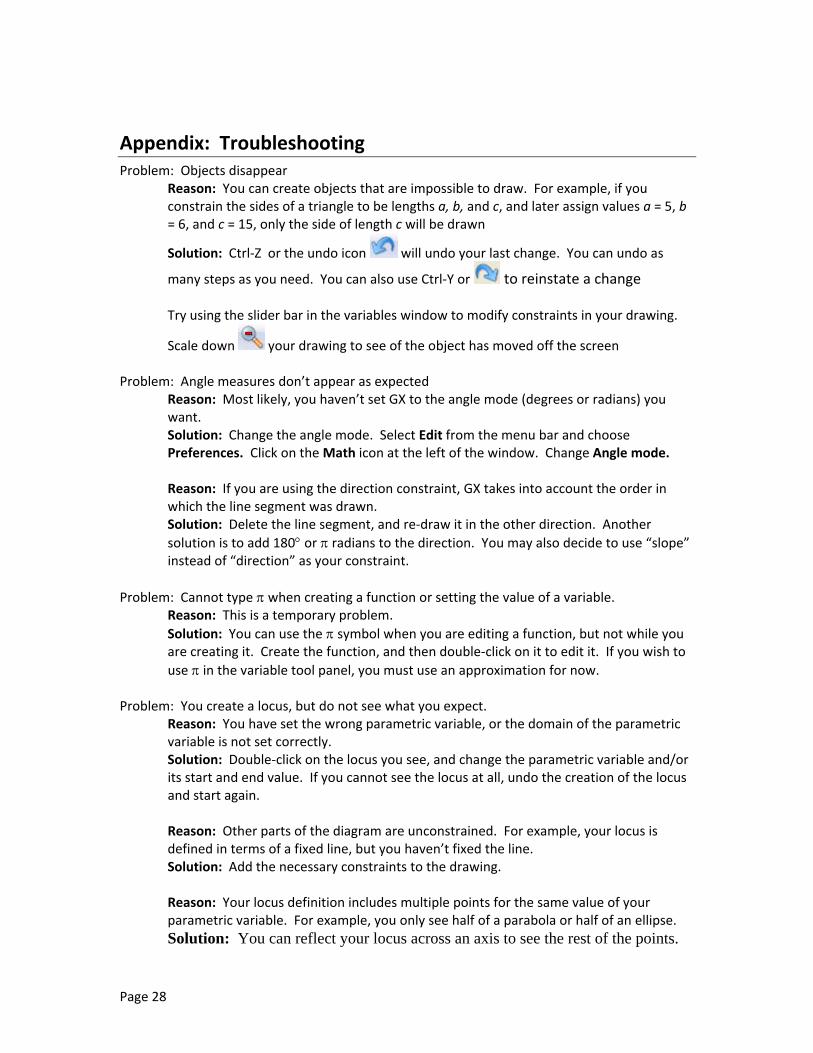
Appendix: Troubleshooting Problem: Objects disappear

Reason: You can create objects that are impossible to draw. For example, if you constrain the sides of a triangle to be lengths a, b, and c, and later assign values a = 5, b = 6, and c = 15, only the side of length c will be drawn

Solution: Ctrl‐Z or the undo icon will undo your last change. You can undo as

many steps as you need. You can also use Ctrl‐Y or to reinstate a change Try using the slider bar in the variables window to modify constraints in your drawing.

Scale down your drawing to see of the object has moved off the screen Problem: Angle measures don’t appear as expected

Reason: Most likely, you haven’t set GX to the angle mode (degrees or radians) you want. Solution: Change the angle mode. Select Edit from the menu bar and choose Preferences. Click on the Math icon at the left of the window. Change Angle mode. Reason: If you are using the direction constraint, GX takes into account the order in which the line segment was drawn. Solution: Delete the line segment, and re‐draw it in the other direction. Another solution is to add 180° or π radians to the direction. You may also decide to use “slope” instead of “direction” as your constraint.

Problem: Cannot type π when creating a function or setting the value of a variable.

Reason: This is a temporary problem. Solution: You can use the π symbol when you are editing a function, but not while you are creating it. Create the function, and then double‐click on it to edit it. If you wish to use π in the variable tool panel, you must use an approximation for now.

Problem: You create a locus, but do not see what you expect. Reason: You have set the wrong parametric variable, or the domain of the parametric variable is not set correctly. Solution: Double‐click on the locus you see, and change the parametric variable and/or its start and end value. If you cannot see the locus at all, undo the creation of the locus and start again. Reason: Other parts of the diagram are unconstrained. For example, your locus is defined in terms of a fixed line, but you haven’t fixed the line. Solution: Add the necessary constraints to the drawing. Reason: Your locus definition includes multiple points for the same value of your parametric variable. For example, you only see half of a parabola or half of an ellipse. Solution: You can reflect your locus across an axis to see the rest of the points.

a constraint in teaching mathematics - geometry …geometryexpressions.com/downloads/lessons/using a...

Documents