Calhoun: The NPS Institutional Archive

Theses and Dissertations Thesis Collection

1967-06

A constrained periodic review model for a

probabilistic reparable-item inventory system.

Hastings, David Ainsworth

Monterey, California. U.S. Naval Postgraduate School

http://hdl.handle.net/10945/11845

brought to you by COREView metadata, citation and similar papers at core.ac.uk

provided by Calhoun, Institutional Archive of the Naval Postgraduate School

NPS ARCHIVE1967HASTINGS, D.

.STRAINED PERIODIC REVIEW MODEL FORA PROBABILISTIC REPARABLE-ITEM

INVENTORY SYSTEM

AVID AINSWORTH HASTINGS

*"" ;.

).'•:'•'.

mil11111$

nniii

iili

G

A CONSTRAINED PERIODIC REVIEW MODEL FOR A

PROBABILISTIC REPARABLE -ITEM INVENTORY SYSTEM

by

David Ainsworth HastingsCaptain, United States Army

B. S. United States Military Academy, 1961

Submitted in partial fulfillment of the

requirements for the degree of

MASTER OF SCIENCE IN OPERATIONS ANALYSIS

from the

NAVAL POSTGRADUATE SCHOOL

June, 1967

n

ABSTRACT

A reparable-item inventory system has two sources of items to

meet demands: from the procurement of new items, and from the re-

pair of damaged or failed items. Further, the system contains two

distinct inventories, one containing procured and repaired ready-for-

issue items and the other containing those failed items awaiting repair.

This thesis develops an approximate model of this general system

assuming that the demand rate and return rate of failed items are

probabilistic. A periodic review policy is assumed for procured items,

and inductions of batches of failed items into repair are assumed to take

place at regularly scheduled intervals of time. The model is structured

as a single coordinated inventory system instead of two separate systems,

one of procured items and one of repaired items. The optimal review

period and "order up to" level for procured items are determined, along

with the optimal time between repair batch inductions.

LIBRARYNAVAL POSTGRADUATE 'SCHOOLMONTEREY, CALIF. 93940

TABLE OF CONTENTS

Section Page

1. Introduction 9

2. Model Formulation 12

2. 1 General 12

2. 2 Order and Review Cost 16

2. 3 Repair Set-up Cost 16

2.4 NRFI Holding Cost 16

2. 5 REI Holding Cost 17

2. 6 RFI Holding Cost 18

2. 7 Units Backordered 21

3. Solution 23

4. Example 26

5. Summary 30

References 31

LIST OF ILLUSTRATIONS

Figure Page

1. Repaired Ready-for-Issue Level Versus Time 13

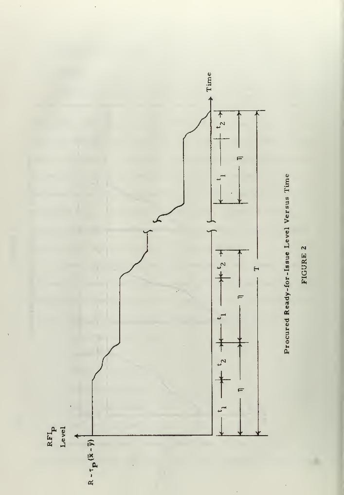
2. Procured Ready-for-Issue Level Versus Time 14

3. Non-Ready-for -Issue Level Versus Time 15

4. Rearrangement of Procured Ready-for-Issue LevelVersus Time 19

TABLE OF SYMBOLS AND ABBREVIATIONS

A - Cost to make one procurement.

A - Set-up cost per repair cycle.

B - Annual budget.

f(x, t) - Density function of the quantity of items, X, demandedin time t .

g(y , t) - Density function of the quantity of items, Y , repairedand returned to RFI in time t .

R

h - Holding cost for ready-for-issue items.

h - Holding cost for non-ready-for-issue items.

J - Cost to make one review.

K - Cost of operating the inventory system.

NRFI - Non-ready-for-issue.

R - Procurement "order up to" quantity.

RFI - That portion of ready-for-issue stock that was procured.

RFI - That portion of ready-for-issue stock that came fromrepair.

S - Expected number of units backordered per unit time.

T - Review cycle time, expressed in years.

V - Number of units backordered.

x - Average annual demand rate.

y - Average annual return rate of repaired items to RFI .R

T] - Fixed cycle time for return of reparable items to ready-

for-issue stock.

II - Lagrange multiplier.

T_ - Procurement leadtime, a given constant.

7

1. INTRODUCTION

There are many ways of categorizing items in an inventory system.

One way is to put all items into one of two areas, either reparable or

non-reparable. In the military, due to the nature of its business, there

is a large number of reparable-type items that represents a considerable

dollar inventory. Realistically, although an item has been classified as

a reparable type of item, not all of a particular type that wear out or

fail can be repaired. For example, the AN/PRC-6 radio is classified as

reparable, but not all the AN/PRC-6 radios that fail or become inopera-

tive can be economically restored to an operating condition. Because of

this, items must be procured from time to time to replenish the overall

inventory system. Understanding this, one realizes that demands can be

satisfied with items that are either procured or that have been returned

to a repair facility and repaired.

Many models have been formulated for the consumable -item inventory

system. These models typically answer the questions of how much to

procure and when to procure in order to minimize cost or shortages.

However, when investigating a reparable-item inventory system, not

only the questions of how much and when to procure must be answered,

but also the questions of how much and when to repair must be answered.

Further, the reparable -item inventory system should be viewed as a

system, rather than separate inventories of procured and repaired ready-

for-issue items.

The system discussed in this paper is reviewed periodically, and a

procurement is made at the time of review. Demand, X , is a random

variable with a density function f(x, t) over the period t. The procure-

ment leadtime, t , is a constant. Repaired items are returned to the

ready-for -issue stock at fixed time intervals of T| , and the quantity

returned during a time t is a random variable, Y , with the density

function g(y, t) . Further, all backorders will be filled.

If the criterion of minimizing total cost per unit time to operate the

system were used, a shortage cost would have to be postulated. This is

extremely difficult to do when discussing military items. How many

dollars does it cost the government or the people of the United States if

a tank, jet fighter, or submarine is inoperable due to the lack of a

spare part? Volumes of literature have been written attempting to

answer this question, for example, Solomon, et al [ 5] . However, no

one has yet provided a satisfactory method for assigning shortage costs

for military equipment. For this reason, the chosen criteria is to

minimize the number of units backordered, subject to an operating cost

budget, and hence avoid postulating a shortage cost. This assumes that

the problem of optimally segmenting an operating cost budget for an

inventory control point into separate operating cost budgets for each type

of item managed by the inventory control point is possible and has been

accomplished.

This model is an approximate approach to the constrained periodic

review system as described. The objective is to determine the optimal

10

order up to level R for procurement, the optimal review period for

procurement, T, and the optimal repair cycle time, T) , such that the

average number of backorders is minimized while maintaining the cost

of operating the system less than or equal to the yearly budget.

11

2. MODEL FORMULATION

2. 1 General

The on-hand inventory of ready-for-issue (RFI) stock may be viewed

as two separate inventories, one consisting of all procured RFI items and

the other consisting of all repaired RFI items. We may consider that all

demands during T| are filled by the RFI stock of repaired items (RFI )R

until it is depleted. At that time, demands are then placed on the pro-

cured RFI stock (RFI ) until the end of the time period T| . At the

beginning of the next time period T) , we receive a variable quantity of

items for RFI , and the process starts over. Figures 1 through 3R ^^

portray this process and the accumulation of the non-ready-for -issue

(NRFI) stock (the notation will be introduced below) .

In order to minimize the expected number" of units backordered,

subject to a budget constraint on operating cost, the total variable oper-

ating cost per unit time must be determined. The relevant components

of the variable cost per unit time needed to be determined are:

(a) procurement order cost;

(b) review cost;

(c) repair set-up cost;

(d) NRFI holding cost;

(e) RFI holding cost;R

( f ) RFI holding cost.

The following subsections develop these costs, the sum of which is the

total variable cost per unit time. Then, the expression for determining

12

T ~7T

CM

tkT CO

(hi

<l>

>,_«

+->

cu

>0)

Y > k J .-H

X A<D wCO cu

CM CO d-i-> 1—

1

1

_yu >—

i

h. k

p

1

0)

_^ tiM

-o<v

ur4

"1'

^;k j

CI.

(MDtJ

-t->

+

f=

4 k

13

J»1Cm £

CO

3CO

>

>

V3co

CO

I

uOVH

I

>.T3

0)

aoufl

uo

CM

w

Da

I*I

IX

i

w

o

en

3en

u4)

>

>

<u

CO

NO<*«

I

>>T3<tJ

CU

i

coZ

15

the expected number of units backordered per unit time is developed.

With this information, a solution to the problem may be determined.

The formulation throughout is approximate, rather than exact. Inventory

holding costs and set-up costs are determined by treating the expected

values of random variables as parameters. The expected number of

units short per unit time expression treats the random variables in the

proper manner, but is only approximate for reasons which will be dis-

cussed when the expression is developed.

2. 2 Order and Review Cost

In the description of the inventory system contained in the introduction,

it was assumed that a procurement order was placed each time a review

was made. The cost associated with placing one order is A . Since the

Ap

review cycle is of fixed length, T , the order cost per unit time is .

JSimilarly, the review cost per unit time is — .

2. 3 Repair Set-up Cost

The repair set-up cost per time period T) is A . Therefore, the

AR

repair set-up cost per unit tune is —-— .

2.4 NRFI Holding Cost

The dimensions of the NRFI holding cost, h , are dollars per unit

year. Therefore, the unit years of stock held in NRFI inventory must

be determined. Figure 3 portrays the NRFI inventory level over time.

The average annual return rate of repaired items is y . Since T| is

expressed in years, the expected height of each triangle is T]y units.

16

*2_11 y

The expected area of each triangle is then ——- . The total numberr>Z -

T] yof unit years of NRFI held for the review period is times the

Tnumber of cycles of length 7| in one review period, —- . Hence, the

holding cost of NRFI per review period is

J- - m hJyTn v T 2HC„ = h, y

T 2 2 T]

Dividing by T yields the holding cost of NRFI per unit time:

h2 ny

HC - -T— . (1)

2. 5 RFL Holding CostR s

The dimensions of RFI holding cost, h , are dollars per unit year.R 1

Hence, to compute the RFI holding cost per unit time, the unit yearsR

of stock held must first be computed. Items are demanded at an average

annual rate of x items. In the determination of NRFI holding cost, it

was seen that the average number of items put into RFI stock per T|R

was T]y . Because all items that are damaged or worn out cannot be

repaired, we would normally expect the quantity demanded to exceed the

quantity repaired. This information is portrayed in Figure 1 .

TlyThe average amount of tune, t , that T) y will fill demands is .

1 x

Thus, the holding cost per T| is

h TOY t h T] yHC.

n 2 2x

and the holding cost per unit time is

h, ry2

HC = — . (2)2x

17

2. 6 RFI Holding CostP B

Again, because of the dimensions of the holding cost, h , the unit

years stocked must be computed. Rearranging the information in

Figure 2 and including a buffer level, which is normally desirable when

dealing with probabilistic demand, the RFI level may be portrayed as

shown in Figure 4 .

The inventory position, defined as the quantity of items on hand plus

on order minus backorders, at the time a review is made is R . A

time t later, all units on order will have arrived and the inventory

level will be R less the leadtime demand. The expected leadtime demand

is t (x - y) . Just prior to the arrival of the next procurement, one

review period later, the inventory level will have decreased an amount

equal to the period's demand. Hence, the inventory level just prior to

the arrival of the next order is R - t (x-y) - T(x-y).

From the preceeding discussion of the RFI holding cost, it wasR

noted that

and

'. - ^

T) (x - y)

2 ~ x

Hence, the area of A is

A.

2 _ 2T (x-y)

2x

18

J* 9

OH

3

i

<1 )L

<

-_J

1—

1

<1

1

I

|X

Oh

I

HI

I

IX

T~

0)

«

>

>V

0)

3

I

S-t

o

"0

a!

T3a)

oo

cvSV

c

W

Dai—

i

i

19

During each period of 7] , the average number of items demanded upon

RFI will equal the average number of demands that RFI could notP R

satisfy, which is 7| ( x - y ) • Therefore, the average height of each

step in the step function in Figure 4 is T\ ( x - y ) .

TEach A. , i = 1 , 2 , . . . , — , will be the product of its height

times t . Thus,

A. = [T(x - y) ]iL

A = [ T (x - y) - T|(S - y)] -32-c x

A = [ T (x - y) - 2Tl(x - y ) ]^X

,

3 x

and, in general,

A. = [ T (x - y) - (i - 1) Tl (x - y) ]

x

The area of the buffer is

Ab

= [R - Tp (x - y) - T (x - y) ] T

The total area, A , is determined by summing the various areas:

the area of the triangle, A ; the buffer area, A ; and the areas of the

Trectangles, A. , i = 1 , 2, . . . , — . Using the relations

NL P = PN

and

N N(N + 1)i- J - o

20

the total area Am may be determined to beT '

AT

=T(x.yM ry -»T)

+ T[R . Tp(5 .-y)] .

TOne notes that the upper limit on the summation of the A.'s is — .

i T|

TThis point may be questionable since there is no guarantee that — will

be an integer. However, if T) is small compared to the review cycle, T,

Tthe error from considering — as an integer is negligible.

The holding cost of RFI per review period is then h A and,

dividing by the review period T, yields the holding cost per unit time.

(x - y) CHy - Tx - 2x T ) _,

HC = hi[R+ _ ]. ,3,

Additionally, there may be some question as to whether or not the

holding cost should be modified to account for the unit years of items

backordered. Because this is an approximate model, we ignore this

term. In light of the objective of this paper, this assumption is only

valid when the budget constraint is not too restrictive.

2. 7 Units Backordered

A procurement order placed at time t will arrive at t + t ,

and the next order will arrive at time t + t + T . At time t , after

the order is placed, the inventory position is R . The next time the

inventory position reaches R is at time t + t + T . Hence, shortages

will occur if the demand on RFI during t + T exceeds R. The

number of units demanded on RFI is X - Y . Let the random variable Z ,

21

with density function h (z , t) , equal X - Y . Now, the number of units

backordered, V , is

if Z £ Rv. {

L Z - R if Z > R

Hence, the expected number of units backordered per unit time, denoted

as S , is

00

S = ^- (Z - R) h(z, t + T) dz . (4)

R

This expression only accounts for the expected number of units back-

ordered at the end of the time period t + T , and hence is only an

approximation to the true expected number of units backordered during

T + T . It does not consider the possibility that units may be back-

ordered at the end of each time period T) , and then filled by the input

of repaired items into RFI . This possibility has been neglected sinceR

it is assumed that if this occurs, the number of items backordered and the

length of time they are backordered are negligible. The duration of such

shortages is only a fraction of T| , which is assumed to be quite small.

It should be noted that if the budget constraint is very restrictive, this

assumption becomes unrealistic.

22

3. SOLUTION

As stated previously, the total variable operating cost per unit time

of the system must be determined in order to minimize S, subject to a

budget constraint. The variable cost per unit time, K, to operate the

system is the sum of the various costs previously derived.

Ap

+ J AR I)y (hj + h

2 )

K =T

+~T~

+2

(x - y) (Tx + 2x t )

+ hi [

RIt J •

(5)

Because demand is probabilistic and the most commonly used functions

to describe demand do not have a finite upper bound, one would normally

assume that the budget constraint would be active.

Assuming that the budget constraint is 'active, the normal method of

solving the problem is through the use of the Lagrange multiplier. The

general Lagragian equation is

L = S + I1(K - B) .

The solution comes from meeting the following conditions:

3L=

_3L=

_3L= Q>

^L= Q

an 3R 3T ' 37)

First, we will determine the optimal value of T] by solving the

= equation for 7] .

dTl

S L S S+ n

^K= Q

o Tl aTl d T)

23

and thus

&Tj n dTl '

From equation 4, we note that S is not a function of T| ; hence. —— =

From equation 5, we see that is

*KAR y (h

i+ V

+ ^3 Tl _2

Solving the —— = for Tl yields6a t]

y

2 A 1/2

Tl =f

^—. (6)

L y(h1

+ h2

)J

Next, we shall look at the condition —=- = . From the generalan s

Lagragian equation the —— = K - B . This implies that K = B .

Hence, solving K = B for R as a function of T yields

i r*(Ap

+ J) ar

y(hi

+ h2

}

i

\ L T \2

-I

(x - y) (Tx + 2xt )

+ — ~ • (7)2 x

To determine the optimal values of R and T one could solve the

= and the —— = simultaneously with equation 7 . However,dT 3R

it is quite easy to solve by selecting several values of T , computing the

associated values of R from equation 7 , and then determining the values

of S from equation 4 using the values of R and T . Throughout these

computations, the optimal value of T| should be used. A plot of S

24

versus T may then be made to indicate the value of T that minimizes S.

With that value of T , equation 7 is then evaluated for R .

The interpretation of the Lagrange multiplier, II , is that it represents

the decrease in the expected number of units backordered per year for

a unit increase in the budget. The value of II may be obtained from the

solution of the —— = . This yields

n =h

i

Th (z, T + T) dz . (8)

R

After obtaining the optimal values of R and T that yield the minimum

expected number of units backordered, II may be evaluated from

equation 8.

25

4. EXAMPLE

The following example is used to demonstrate the nature of the

solutions presented by the model, and to explore the trade-off between

procurement order and review costs and holding costs.

Let demand and the quantity of items returned to RFI be normallyR

distributed with means of 1, 000 units per year and 900 units per year,

and standard deviations of 30 units per year and 50 units per year,

respectively. Procurement leadtime, t , is . 5 years. The relevant

costs are: A = $750, A = $100, J = $250, h - $200, andPR 1

h = $20 . The two random variables, X and Y , are assumed to be

independent. Also, demand during T is independent of demand during

T ; and the quantity of items returned to RFI during T is independentP R

of the quantity of items returned to RFI during t . Therefore, theR P

random variable Z is normally distributed with mean 100(t + T)

1/2and standard deviation equal to [ (t + T) 3400

Let B = $20, 000 . Following the procedure outlined in section 3,

the first step is to determine Tj . Evaluating equation 6 yields

- 27) = 3. 18x10 years, which is approximately 12 days. Next, we solve

equation 7 for various values of R for selected values of T . If

T = . 1 years, R = 73 units; if T = . 5 years, R = 133 units; and

if T = 1 year, R = 1 63 units. Next, using these values of R and T,

determine the associated values of S. For this example, the general

solution of S is

26

S = — I c ( ) '+ (z - R) § ( )

where2

r

0(r) = e

V2n

|(r) = 0(x) dxr

and z is the mean of Z , and a is the standard deviation of Z

The associated values of S are as follows:

R

0. 1 73 123

0. 5 133 21

1. 163 22

From plotting these values, we see that the minimum S occurs near

T = . 8 years. Evaluating R for T = . 7 , . 8 , and . 9 years and evalu-

ating the associated values of S, the following results were obtained.

T R S

0. 7 146 21

0. 8 152 20

0.9 158 22

Thus, the minimum expected number of units backordered per year is 20

when the review cycle is . 8 years, the procurement order up to level is

27

152 units, and the cycle time for the receipt of repaired items is

- 23. 18x10 years. The Lagrange multiplier, II , may now be evaluated

_ 3from equation 8. This yields II = 2. 31x10 units per dollar.

Various budget levels were considered to investigate the changes in

the expected number of units backordered per year, S. The results

are tabulated below. The mean demand during t + T , denoted as x,

and the expected number of units backordered per review period, de-

noted as Sm , are also shown.T

B T R x S S

$10,000 4.0 276 450 45 180

$15,000 0.9 133 140 35 32

$20,000 0.8 152 130 20 16

The cost to operate the repair side of the system per year, with no

review and procurement order costs, is approximately $6, 000. With

this budget level, the expected number of units backordered per year

is 100. When the budget is increased to $10, 000 , the review cycle is

very long because it is profitable to put the majority of the additional

money into holding procured items, instead of sustaining the high procure'

ment order and review costs frequently. As the budget is increased to

$15, 000 , the review cycle decreases to . 9 years, indicating that the

system can afford to review and order procurement more often in order

to achieve an economic balance between ordering and reviewing and

holding costs. An increase of the budget by one-third to $20, 000 yields

28

only a slight decrease of the review period to . 8 years, thereby puttirj

most of the increased budget into safety stock.

29

5. SUMMARY

We have discussed a reparable-item inventory system with random

demand. A periodic review policy was assumed for procured items,

while inductions of carcasses were assumed to take place at regularly

spaced intervals. As the accumulation rate of NRFI carcasses was

assumed random, the repair batch sizes were also random. The ob-

jective was to determine the optimal procurement review period T,

the optimal procurement order up to level R, and the optimal repair

time period7] , in order to minimize the expected number of units

backordered per unit time, subject to an annual operating budget

constraint. The model developed is an approximate model. The solu-

tions presented are sensitive to the assumptions that 7] is small com-

pared to T, and that the expected unit years of items backordered are

small. Obviously, the model is also sensitive to the restrictiveness of

the budget constraint.

As discussed in the introduction, the purpose of minimizing S sub-

ject to a budget constraint was to avoid postulating a shortage cost.

However, even though a shortage cost may not be stated by a decision-

maker or an item manager, it is implied as soon as a specific operating

budget is established. We noted in section 3 that n , defined as the

Lagrange multiplier, may be interpreted as the decrease in the expected

number of units backordered per year for a unit increase of the budget.

Therefore, — is the shortage cost, which would yield the same decision

rules if the more common criteria of minimum cost per unit time were used.

30

REFERENCES

[ 1] Hadley, G. , and T. M. Whiten. Analysis of Inventory Systems,

Prentice- Hall, 1963.

[2] Hatchett, J. W. , and P. F. McNall. "A Repairable ItemInventory Model", Master's Thesis, Naval PostgraduateSchool, Monterey, California, October, 1966.

[3] Hoekstra, D. "Supply Management Models for Repairable Items",

Inventory Research Office, U. S. Army Supply andMaintenance Command, Frankford Arsenal, Philadelphia,

Pennsylvania; a paper presented at the Fifth U. S. ArmyOperations Research Symposium, Fort Monmouth,New Jersey, March, 1966.

[4] Schrady, D. A. "A Deterministic Inventory Model for ReparableItems", paper to appear in Naval Research Logistics

Quarterly .

[5] Solomon, Fennel, and Denicoff. "A Method of Determining the

Military Worth of Spare Parts", Logistics Research Project,

George Washington University, T-82 / 58, Washington, D. C. ,

April, 1958.

31

+ INITIAL DISTRIBUTION LIST

> , No. Copies

1. Defense Documentation Center 20

Cameron Station

Alexandria, Virginia 22314

2. Library 2

Naval Postgraduate SchoolMonterey, California 93940

3. Professor David A. Schrady... 5

822 Casanova AvenueMonterey, California 93940

4. Captain David A. Hastings 1

7605 Range RoadAlexandria, Virginia

5. Commander James A. Gillespie, SC, USN 1

Director, Operations Analysis Department (Code 97)

Fleet Material Support Office

Naval Supply DepotMechanicsburg, Pennsylvania 17055

6. Lieutenant Commander Richard De Winter 1

Navy Aviation Supply Office »' •

700 Robbins AvenuePhiladelphia, Pennsylvania 19111

Chief of Naval Operations (OP 96)

Navy DepartmentWashington, D. C. 20350

32

UNCLASSIFIEDSecurity Classification

DOCUMENT CONTROL DATA • R&D(Maouhty etmaalhcmtlon ot titla, body ot abatract and Indexing annotation muat ba antarad whan tha ovarall import la claaaillad)

I. ORIGIN A TIN ACTIVITY (Cotpomta author)

Naval Postgraduate School

Monterey, California 93940

2«. REPORT SECURITY CLASSIFICATION

UNCLASSIFIED2 b. CROUP

>. REPORT TITLE

A CONSTRAINED PERIODIC REVIEW MODEL FOR APROBABILISTIC REPARABLE -ITEM INVENTORY SYSTEM

4. DESCRIPTIVE NOTES (Typa ot raport and Inctualva dataa)

Master's Thesis5 AUTHORfSJ (Laat nama, lint name. Initial)

Hastings, David A. , Captain, United States Army

6. REPORT DATE

June, 1967

7«- TOTAL NO. OP

31

7b. NO. OF REFS

5

• «. CONTRACT OR 6RANT NO.

a, PROJECT NO.

• «. ORIGINATOR'S REPORT NUMEERfSj

16. other REPORT **Q(3) (A ny otfiar numbara that may ba aaaignad

10. A V A IL ABILITY/LIMITATION NOTICESmM-WM

II. SUPPLEMENTARY NOTES 12. SPONSORING MILITARY ACTIVITY

Naval Postgraduate SchoolMonterey, California 93940

13. ABSTRACT

A reparable -item inventory system has two sources of items to meetdemands: from the procurement of new items, and from the repair ofdamaged or failed items. Further, the system contains two distinctinventories, one containing procured and repaired ready-for-issue itemsand the other containing those failed items awaiting repair. This thesisdevelops an approximate model of this general system assuming that thedemand rate and return rate of failed items are probabilistic. A periodicreview policy is assumed for procured items, and inductions of batches offailed items into repair are assumed to take place at regularly scheduledintervals of time. The model is structured as a single coordinated inventorysystem instead of two separate systems, one of procured items and one ofrepaired items. The optimal review period and "order up to" level forprocured items are determined, along with the optimal time between repairbatch inductions.

DD .KK-1473 UNCLASSIFIEDSecurity Classification

•H

UNCLASSIFIEDSecurity Classification

KEY WO R DS

Reparable

Inventory Model

Ready -for -Is sue

Non-Ready-for-Issue

.**«.

.-*£ «i; ... aifc.'.' ant* :^x'

.a,-«e*a.*'" - —-t*- -- <

,J-V^Ait) *» .

'-^-iHMJIti'

DD, F.°o

RvM473 <back) UNCLASSIFIEDS/N 0101-807-6821 Security Classification A-31 409

34

thesH313

3 2768 00414772 8

DUDLEY KNOX LIBRARY

n*

iiff

Julivvrnm

mmfflflfeflftlJI

UlflVH

mi

mu«Sfl NUtt

SUOfitHtHl>

!fcWHSHi

tint iflL

tstnfiti•" v

\MW\

;