1225 Observatory Drive, Madison, Wisconsin 53706

608-262-3581 / www.lafollette.wisc.edu The La Follette School takes no stand on policy issues; opinions expressed

in this paper reflect the views of individual researchers and authors.

Robert M.

La Follette School of Public Affairs at the University of Wisconsin-Madison Working Paper Series La Follette School Working Paper No. 2013-009 http://www.lafollette.wisc.edu/publications/workingpapers

A Consideration of Patterns of Intra-Industry Trade: Why Do Countries Export and Import More/Less in the Same Industry?

Isao Kamata La Follette School of Public Affairs, University of Wisconsin–Madison

ikamata@lafollette.wisc.edu

A Consideration of Patterns of Intra-Industry Trade: Why Do Countries Export and Import More/Less in the Same Industry?

Isao Kamata § University of Wisconsin–Madison

This version: March 15, 2013

Abstract It is observed in data that in most manufacturing industries a country’s exports and imports, measured in values per GDP within an industry, are positively correlated. This indicates that the countries exporting more (less) in an industry tend to import more (less) in the same industry, relative to the size of their economy. In this paper I employ the model of intra-industry trade that has been widely used in the literature, also allowing transport costs and price asymmetry across countries, to examine whether and how the model can explain such positive correlations between a country’s export and import in the same industry. The theoretical prediction of the model is that a country’s export and import per GDP could both be smaller (greater) in the same industry if the country‘s production share in the world total in that industry and its GDP share in the world are both greater (smaller). The result of the data analysis shows, however, that the model can predict only smaller or negative correlations in many industries, while countries’ production sizes and GDPs are almost perfectly positively correlated. This result seems to imply that an alternative mechanism missed in the conventional model is needed to explain the pattern of intra-industry trade. Keywords: Intra-industry trade; Export-import correlation; New Trade Theory JEL classification: F10, F12, F14,

§ I am particularly grateful to Alan Deardorff and Juan Carlos Hallak for extensive discussions and also thank Gary Saxonhouse for valuable and helpful comments. I am solely responsible for all remaining errors.

1

1. Introduction The law of comparative advantage is the oldest and the most prevailing proposition in the theory of international trade. The law states that a country will specialize in production and export of the goods in which it has an advantage in relative production costs due to difference in technology (in the Ricardian sense) or difference in relative factor abundance (in the sense of Heckscher-Ohlin (H-O)); and will import the other goods.1 This provides a sharp prediction of patterns of international trade in the case in which goods are homogeneous: a country will not import the goods that it exports, or vice versa, and thus there is no intra-industry trade. The “new theory” of international trade such as the work by Krugman (1979, 1980) introduced the market structure of monopolistic competition to explain the intra-industry trade that was observed in reality. Helpman and Krugman (1985) incorporated the monopolistic competition model with the traditional H-O framework, but the original prediction by the law of comparative advantage is still valid in their model, in a slightly weaker manner: that is, a country is expected to be a net exporter of the industry in which it has comparative advantage. The expected cross-country pattern of trade within an industry, then, would be such that, if a country exports more in an industry, the country should import less in that industry. What do data tell about the pattern? Table 1 shows the correlations between the values of exports and imports across countries within each of the manufacturing industries classified by the 3-digit ISIC (Revision 2).2 The values of exports and imports are divided by GDP of each country in order to adjust for the size of the economy. The result is surprising: in most of the manufacturing industries, exports and imports of the countries are positively correlated, and the correlations are fairly strong in some industries. This implies that the countries that export more (relative to the size of the economy) in an industry tend to import more in the same industry, and vice versa. This seems to be the opposite to what is expected according to the law of comparative advantage.3 The model of intra-industry trade with monopolistic competition of differentiated products has been widely used in the literature, such as Romalis (2004). The purpose of this

1 Indeed in some cases countries will specialize incompletely and the law of comparative advantage cannot predict the exact patterns of countries’ specialization. Deardorff (1980) has a great summary on this. 2 Description of the data is in Section 5 of this paper. 3 The correlation cannot be positive if products are homogeneous and thus there is no intra-industry trade. That is, when a country exports in an industry (Xc

i>0), it does not import in that industry at all (Mci=0), or vice

versa. Thus, the covariance Cov(Xci,Mc

i) ≡ E[XciMc

i]-E[Xci]·E[Mc

i] is definitely non-positive since the first term is zero but E[Xc

i]≥0 and E[Mci]≥0 so that the second term is negative. Note that the signs of covariance

and correlation coefficient are the same.

1

1. Introduction

The law of comparative advantage is the oldest and the most prevailing proposition

in the theory of international trade. The law states that a country will specialize in

production and export of the goods in which it has an advantage in relative production

costs due to difference in technology (in the Ricardian sense) or difference in relative factor

abundance (in the sense of Heckscher-Ohlin (H-O)); and will import the other goods.1 This

provides a sharp prediction of patterns of international trade in the case in which goods are

homogeneous: a country will not import the goods that it exports, or vice versa, and thus

there is no intra-industry trade. The “new theory” of international trade such as the work by

Krugman (1979, 1980) introduced the market structure of monopolistic competition to

explain the intra-industry trade that was observed in reality. Helpman and Krugman (1985)

incorporated the monopolistic competition model with the traditional H-O framework, but

the original prediction by the law of comparative advantage is still valid in their model, in a

slightly weaker manner: that is, a country is expected to be a net exporter of the industry in

which it has comparative advantage. The expected cross-country pattern of trade within an

industry, then, would be such that, if a country exports more in an industry, the country

should import less in that industry.

What do data tell about the pattern? Table 1 shows the correlations between the

values of exports and imports across countries within each of the manufacturing industries

classified by the 3-digit ISIC (Revision 2).2 The values of exports and imports are divided

by GDP of each country in order to adjust for the size of the economy. The result is

surprising: in most of the manufacturing industries, exports and imports of the countries are

positively correlated, and the correlations are fairly strong in some industries. This implies

that the countries that export more (relative to the size of the economy) in an industry tend

to import more in the same industry, and vice versa. This seems to be the opposite to what

is expected according to the law of comparative advantage.3

The model of intra-industry trade with monopolistic competition of differentiated

products has been widely used in the literature, such as Romalis (2004). The purpose of this

1 Indeed in some cases countries will specialize incompletely and the law of comparative advantage cannot

predict the exact patterns of countries’ specialization. Deardorff (1980) has a great summary on this. 2 Description of the data is in Section 5 of this paper. 3 The correlation cannot be positive if products are homogeneous and thus there is no intra-industry trade.

That is, when a country exports in an industry (Xci>0), it does not import in that industry at all (Mc

i=0), or vice

versa. Thus, the covariance Cov(Xci,Mc

i) ≡ E[Xc

iMc

i]-E[Xc

i]∙E[Mc

i] is definitely non-positive since the first

term is zero but E[Xci]≥0 and E[Mc

i]≥0 so that the second term is negative. Note that the signs of covariance

and correlation coefficient are the same.

2

paper is to examine whether this conventional model can explain the positive correlation

between a country’s exports and imports in the same industry that is observed in data. I start

with the model under a conventional (but restrictive) set of assumptions such as free trade

and symmetric prices, and later introduce a more general form by allowing transport costs

and price differences across countries in order to see whether such relaxing affects the

prediction of the model. The restrictive version of the model is then tested using

cross-country data on manufacturing production, trade, and GDP by comparing the

predicted correlations to the actual. The relaxed version is not tested because it involves

variables that are not observable in the data. Instead, a possible procedure for testing the

relaxed version of the model without having those unobservable variables is proposed.

The key finding of this paper is the following: The theoretical results from the

comparative statics of the model indicate that a country’s exports and imports per GDP

could both be smaller (greater) in the same industry if the country‘s production share in the

world total in that industry and the country’s GDP share in the world are both greater

(smaller). The data analysis shows, however, that the model can predict only smaller or

negative correlations in many manufacturing industries, while the sizes of the countries’

production and their GDPs are almost perfectly positively correlated. This result seems to

imply that an alternative mechanism that is missed in the conventional model is needed to

explain the pattern of intra-industry trade.

The organization of the paper is as follows: In Section 2 a piece of evidence is

presented to show that the positive correlation between exports and imports is robust

regardless the level of industry aggregation. Section 3 presents the model and derives

expressions of key variables. Section 4 shows comparative statics of the key variables to

show how the model predicts ‘co-movement’ of a country’s exports and imports. Section 5

performs a data analysis for the restrictive version of the model, together with description

of the data employed. Concluding Section 6 discusses the results.

2. Is It Due to Aggregation?

Finger (1975) claimed that intra-industry trade would disappear if commodities

were better-classified at a more disaggregated level. Likewise, one might ask whether the

positive cross-country correlation between exports per GDP and imports per GDP within

the same industry shown in Table 1 is simply due to the aggregation of industries, and

whether, at a less aggregated level, countries do indeed import different goods from those

3

they export?

In order to check whether this is the case or not, let us see the correlations at as

disaggregated level as possible. Although my analysis overall in this paper is based on the

industry classification (the International Standard Industrial Classification: ISIC), the data

at a disaggregated-level ISIC are not available for multiple countries. Therefore, in this

section I employ United Nations data on world trade classified by the Standard

International Trade Classification (SITC: Revision 2)4 and calculate the correlation

coefficient between exports per GDP and imports per GDP within each commodity by 3-,

4-, and 5-digit SITC.5 In addition, I draw on the data for the 6-digit Harmonized System

(HS: 1992) from the same database for further disaggregating. The number of commodities

included in the data for SITC at each digit level is 239, 786, and 1,464 respectively, and the

number of countries is 97, 95, and 94, respectively. For the 6-digit HS, the number of

commodities is 5,035 and the number of countries is 31.6

Figure 1 presents the histograms showing the distribution of the number of

commodities over the level of correlations between exports and imports per GDP for each

level of the aggregation. As shown in the figure, the distributions of the correlation

coefficients do not change much by the level of aggregation, and the correlations are

positive in most commodities. This shows that, at least for any of the aggregation levels that

the data allow, the positive correlation between exports and imports (both per GDP) is

robust. The aggregation may not matter for this pattern.

3. The Model

The model that I present here is a version of the monopolistic competition model

of intra-industry trade employed by Romalis (2004). I first present the common

assumptions that the model is based on throughout this paper, and derive common elements

of the model. I then consider three cases, ranging from the most restrictive assumptions to

the least restrictive assumptions, to derive three versions of the model.

(1) Common Assumptions

The assumptions that are common to all the versions of the model are the

4 The source of the data is United Nations Commodity Trade Statistics Database, or UN Comtrade (on-line). 5 5-digit is the most disaggregated level for SITC (Rev.2) available in UN Comtrade. 6 The data for HS are available only for a limited number of countries, which are mainly the OECD members.

4

following:

1. There are M (>1) countries (c = 1, 2, …, M) in the world (the multi-country setting).

(Note, however, that in the following parts of this paper I also apply the two-country

setting (country c and “the rest of the world”) in order to examine the model in a simpler

manner.)

2. All consumers in all countries have identical Cobb-Douglas preferences over industries,

so that consumers’ expenditure shares on each industry are constant for all prices and

incomes. bi shows the expenditure share for industry i. That is;

lni i

i

U b Q ; (1)

1i

i

b . (2)

3. Each industry is monopolistically competitive. That is, each industry consists of a

number of varieties that are imperfect substitutes for each other, and each firm produces

one variety. nci denotes the number of firms in industry i in country c, and N

i denotes the

world total number of firms in the industry: that is;

Mi i

c

c

N n . (3)

4. Consumers have identical preferences with a constant elasticity of substitution (CES)

over varieties within an industry. By interpreting Qi in Equation (1) above as consumers’

sub-utility, this is shown by:

1/[ ( ( )) ]

i

i i

Ni D

c

i

Q q

; (4)

where qcD(ω) is the quantity of product (variety) ω in industry i demanded by consumers,

θi = 1 - 1/σi where σi is the elasticity of substitution among varieties in the industry (σi >

1).

5. There may be transport costs for international trade. For modeling convenience, I use the

“iceberg” form of transport costs that may vary across industries, according to which, for

each industry i, τi ≥1 units of output must be shipped from one country for one unit to

reach any other country.

5

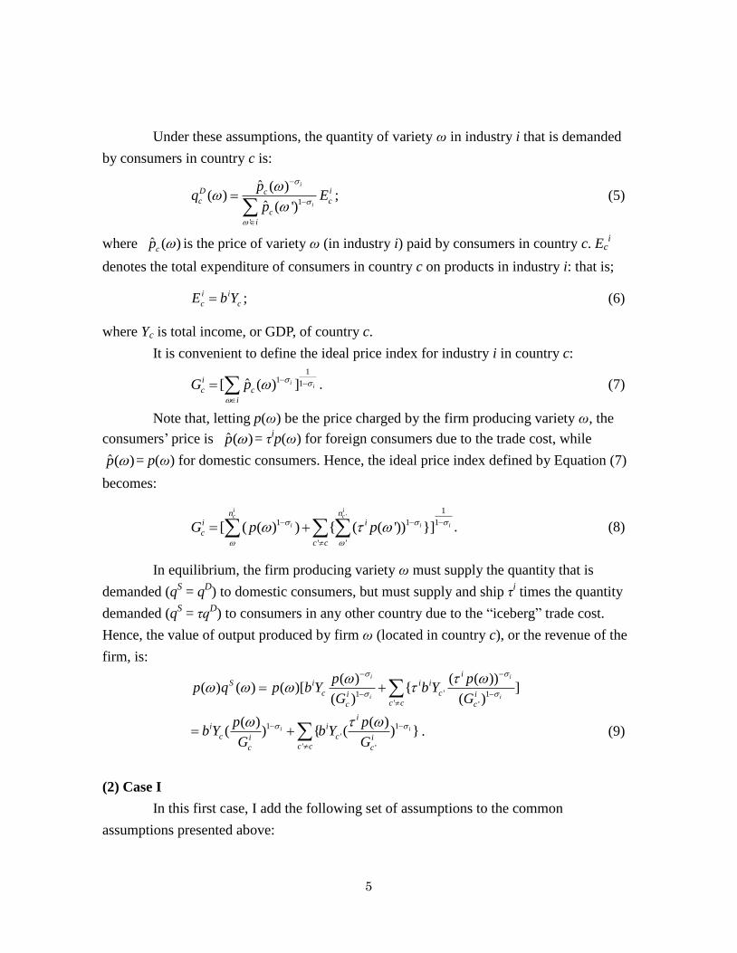
Under these assumptions, the quantity of variety ω in industry i that is demanded

by consumers in country c is:

1

'

ˆ ( )( )

ˆ ( ')

i

i

D icc c

c

i

pq E

p

; (5)

where ˆ ( )cp is the price of variety ω (in industry i) paid by consumers in country c. Eci

denotes the total expenditure of consumers in country c on products in industry i: that is;

i i

c cE b Y ; (6)

where Yc is total income, or GDP, of country c.

It is convenient to define the ideal price index for industry i in country c:

11 1ˆ[ ( ) ]i

ii

c c

i

G p

. (7)

Note that, letting p(ω) be the price charged by the firm producing variety ω, the

consumers’ price is ˆ ( )p = τip(ω) for foreign consumers due to the trade cost, while

ˆ ( )p = p(ω) for domestic consumers. Hence, the ideal price index defined by Equation (7)

becomes:

'1

1 1 1

' '

[ ( ( ) ) { ( ( ')) }]

i ic c

i i i

n ni i

c

c c

G p p

. (8)

In equilibrium, the firm producing variety ω must supply the quantity that is

demanded (qS = q

D) to domestic consumers, but must supply and ship τ

i times the quantity

demanded (qS = τq

D) to consumers in any other country due to the “iceberg” trade cost.

Hence, the value of output produced by firm ω (located in country c), or the revenue of the

firm, is:

'1 1' '

( ) ( ( ))( ) ( ) ( )[ { ]

( ) ( )

i i

i i

iS i i i

c ci ic cc c

p pp q p b Y b Y

G G

1 1

'

' '

( ) ( )( ) { ( ) }i i

ii i

c ci ic cc c

p pb Y b Y

G G

. (9)

(2) Case I

In this first case, I add the following set of assumptions to the common

assumptions presented above:

6

I-6. Production technologies of all varieties in an industry are identical in the world.

I-7. Free and frictionless international trade: countries costlessly trade their products each

other. That is, τi = 1 for any industry i.

I-8. In equilibrium, the producers’ prices of all varieties in an industry are equal to each

other. That is, ( ) ip p i .

Note that, under these assumptions, the output of each variety (or the size of each firm) in

an industry is identical: qS(ω) = q

iS i .

With these additional assumptions, Equations (8) and (9) above are modified to the

following version for this Case I (from now on, for simplicity, the output quantity qS is

denoted by q without the script S):

1 1

1 1 1 1

'

'

[ ( ) ( ) ] ( )i i i ii i i i i i i i

c c c

c c

G G n p n p p N

c ; (8-I)

1( )

Mi i i

cic

p q b YN

. (9-I)

That is, all firms in an industry have the same size and revenue.

Now I derive the expressions for the values of production, exports, and imports of

a country in an industry for this Case I. Since my interest is in comparison of values of

exports and imports in an industry, I suppress the script i denoting an industry from the

expressions below. Let VQc, VXc, and VMc be the values of production, exports, and imports

of country c in an industry, respectively; and VQw, VXw, and VMw be those of the world

(total). Then;

( )M

cc c c

c

nVQ n pq b Y

N ; (10-I)

'

'

( )cc c

c c

nVX b Y

N

; (11-I)

'

' ( )c

c c cc c c

nN n

VM bY bYN N

. (12-I)

Equation (11-I) is so because VXc is the total value of the varieties produced in and shipped

from country c to all other countries. Equation (12-I) is because VMc is the total value of the

foreign varieties (for country c) bought by consumers in country c.

7

Therefore, for each country c, the values of exports and imports in an industry, as

ratios to the country’s GDP, are, respectively:7

1c w cc

c w c

VX VQ yx

Y Y y

; (13-I)

(1 )c wc

c w

VM VQx

Y Y ; (14-I)

where xc ≡ VQc/VQw is country c’s share of world production in the industry, and yc ≡ Yc/Yw

is country c’s share of the world income (GDP). Note that, in this Case I, since the values of

output (or revenues) of all firms in an industry are identical, xc is equal to country c’s share

of the number of firms in the industry to the world total number of firms: xc = ncpq/Npq =

nc/N.

Correlation Coefficient

In this Case I, the correlation coefficient between the values of exports and imports

per GDP within an industry, ρi(VXc

i/Yc

i, VMc

i/Yc

i), is derived as follows:

8

1 1( , ) ( ,1 ) ( , )

i ii i i i i i ic c c c

c c c c

c c c c

VX VM y yx x x x

Y Y y y

. (15-I)

(3) Case II

In this second case, I keep the same set of assumptions as in Case I above, except

one: I introduce a positive trade cost in the model rather than free trade. That is, assumption

I-7 in Case I is replaced with the following:

II-7. There is a transport cost for international trade in industry i: i.e., τi > 1.

The other two assumptions I-6 and I-8 are kept in this Case II.9

With this second set of assumptions added to the common assumptions 1 through 5,

Equations (8) and (9) are modified into the following version for this Case II (suppressing

the script i for the industry):10

1

1[ ( )]c c cG p n T N n where 1T ; (8-II)

7 See Appendix C-1 for derivation of Equations (13-I) and (14-I). 8 See Appendix C-2 for the details of the derivation of the correlation coefficient. 9 Note that the values of output (pq) are identical for all firms in an industry also in this Case II. 10 See Appendix C-1 for derivation of the following equations (8-II) through (14-II).

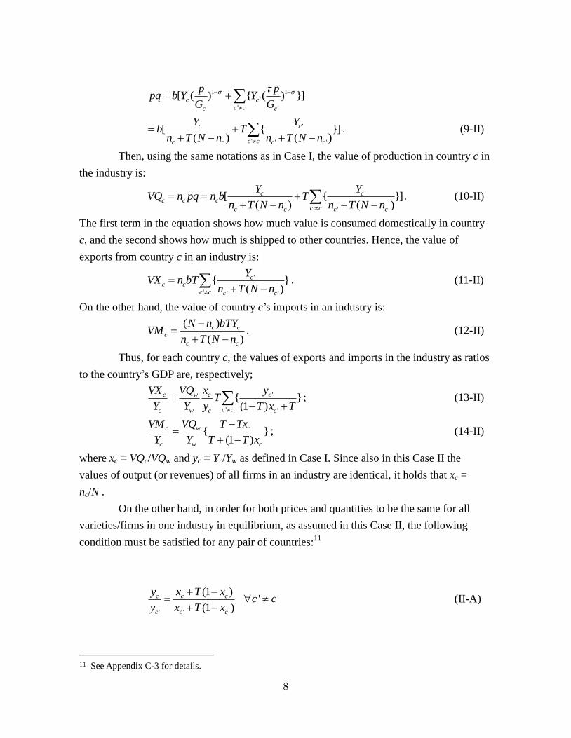
8

1 1

'

' '

[ ( ) { ( ) }]c c

c cc c

p ppq b Y Y

G G

'

' ' '

[ { }]( ) ( )

c c

c cc c c c

Y Yb T

n T N n n T N n

. (9-II)

Then, using the same notations as in Case I, the value of production in country c in

the industry is:

'

' ' '

[ { }]( ) ( )

c cc c c

c cc c c c

Y YVQ n pq n b T

n T N n n T N n

. (10-II)

The first term in the equation shows how much value is consumed domestically in country

c, and the second shows how much is shipped to other countries. Hence, the value of

exports from country c in an industry is:

'

' ' '

{ }( )

cc c

c c c c

YVX n bT

n T N n

. (11-II)

On the other hand, the value of country c’s imports in an industry is:

( )

( )

c cc

c c

N n bTYVM

n T N n

. (12-II)

Thus, for each country c, the values of exports and imports in the industry as ratios

to the country’s GDP are, respectively;

'

' '

{ }(1 )

c w c c

c cc w c c

VX VQ x yT

Y Y y T x T

; (13-II)

{ }(1 )

c w c

c w c

VM VQ T Tx

Y Y T T x

; (14-II)

where xc ≡ VQc/VQw and yc ≡ Yc/Yw as defined in Case I. Since also in this Case II the

values of output (or revenues) of all firms in an industry are identical, it holds that xc =

nc/N .

On the other hand, in order for both prices and quantities to be the same for all

varieties/firms in one industry in equilibrium, as assumed in this Case II, the following

condition must be satisfied for any pair of countries:11

' ' '

(1 )

(1 )

c c c

c c c

y x T x

y x T x

'c c (II-A)

11 See Appendix C-3 for details.

9

'

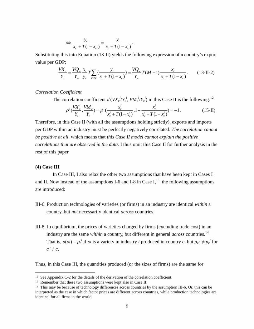
' '(1 ) (1 )

c c

c c c c

y y

x T x x T x

.

Substituting this into Equation (13-II) yields the following expression of a country’s export

value per GDP:

'

{ } ( 1)(1 ) (1 )

c w c c w c

c cc w c c c w c c

VX VQ x y VQ xT T M

Y Y y x T x Y x T x

. (13-II-2)

Correlation Coefficient

The correlation coefficient ρi(VXc

i/Yc

i, VMc

i/Yc

i) in this Case II is the following:

12

( , ) ( ,1 ) 1(1 ) (1 )

i i i ii ic c c c

i i i i

c c c c c c

VX VM x x

Y Y x T x x T x

. (15-II)

Therefore, in this Case II (with all the assumptions holding strictly), exports and imports

per GDP within an industry must be perfectly negatively correlated. The correlation cannot

be positive at all, which means that this Case II model cannot explain the positive

correlations that are observed in the data. I thus omit this Case II for further analysis in the

rest of this paper.

(4) Case III

In Case III, I also relax the other two assumptions that have been kept in Cases I

and II. Now instead of the assumptions I-6 and I-8 in Case I,13

the following assumptions

are introduced:

III-6. Production technologies of varieties (or firms) in an industry are identical within a

country, but not necessarily identical across countries.

III-8. In equilibrium, the prices of varieties charged by firms (excluding trade cost) in an

industry are the same within a country, but different in general across countries.14

That is, p(ω) = pci if ω is a variety in industry i produced in country c, but pc’

i ≠ pc

i for

c’ ≠ c.

Thus, in this Case III, the quantities produced (or the sizes of firms) are the same for

12 See Appendix C-2 for the details of the derivation of the correlation coefficient. 13 Remember that these two assumptions were kept also in Case II. 14 This may be because of technology differences across countries by the assumption III-6. Or, this can be

interpreted as the case in which factor prices are different across countries, while production technologies are

identical for all firms in the world.

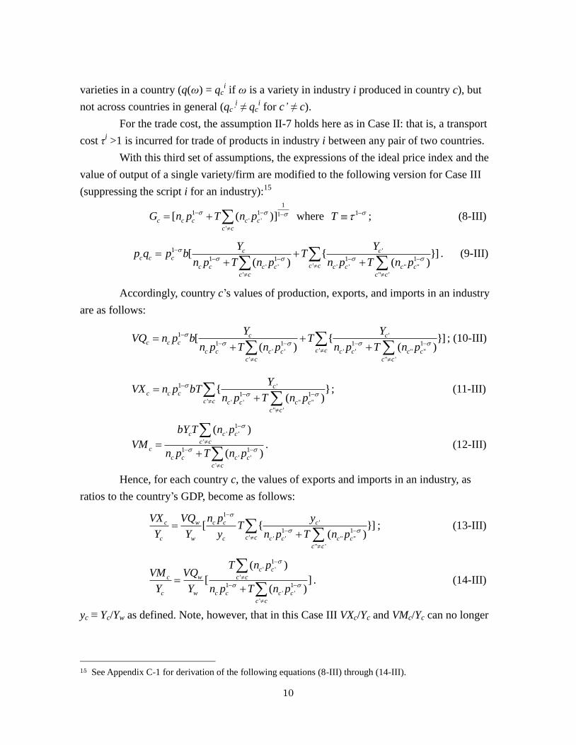
10

varieties in a country (q(ω) = qci if ω is a variety in industry i produced in country c), but

not across countries in general (qc’i ≠ qc

i for c’ ≠ c).

For the trade cost, the assumption II-7 holds here as in Case II: that is, a transport

cost τi >1 is incurred for trade of products in industry i between any pair of two countries.

With this third set of assumptions, the expressions of the ideal price index and the

value of output of a single variety/firm are modified to the following version for Case III

(suppressing the script i for an industry):15

1

1 1 1' '

'

[ ( )]c c c c c

c c

G n p T n p

where 1T ; (8-III)

1 '

1 1 1 1'' ' ' ' " "

' " '

[ { }]( ) ( )

c cc c c

c cc c c c c c c c

c c c c

Y Yp q p b T

n p T n p n p T n p

. (9-III)

Accordingly, country c’s values of production, exports, and imports in an industry

are as follows:

1 '

1 1 1 1'' ' ' ' " "

' " '

[ { }]( ) ( )

c cc c c

c cc c c c c c c c

c c c c

Y YVQ n p b T

n p T n p n p T n p

; (10-III)

1 '

1 1' ' ' " "

" '

{ }( )

cc c c

c c c c c c

c c

YVX n p bT

n p T n p

; (11-III)

1

' '

'

1 1

' '

'

( )

( )

c c c

c cc

c c c c

c c

bY T n p

VMn p T n p

. (12-III)

Hence, for each country c, the values of exports and imports in an industry, as

ratios to the country’s GDP, become as follows:

1

'

1 1' ' ' " "

" '

[ { }]( )

c w c c c

c cc w c c c c c

c c

VX VQ n p yT

Y Y y n p T n p

; (13-III)

1

' '

'

1 1

' '

'

( )

[ ]( )

c c

c w c c

c w c c c c

c c

T n pVM VQ

Y Y n p T n p

. (14-III)

yc ≡ Yc/Yw as defined. Note, however, that in this Case III VXc/Yc and VMc/Yc can no longer

15 See Appendix C-1 for derivation of the following equations (8-III) through (14-III).

11

usefully be expressed using / /M

c c w c c c c c c

c

x VQ VQ n p q n p q since the values of output of

firms in an industry are different across countries (pc’qc’ ≠ pcqc for c’ ≠ c), so that xc is not

equal to the share in the number of firms, nc/N, in this case.

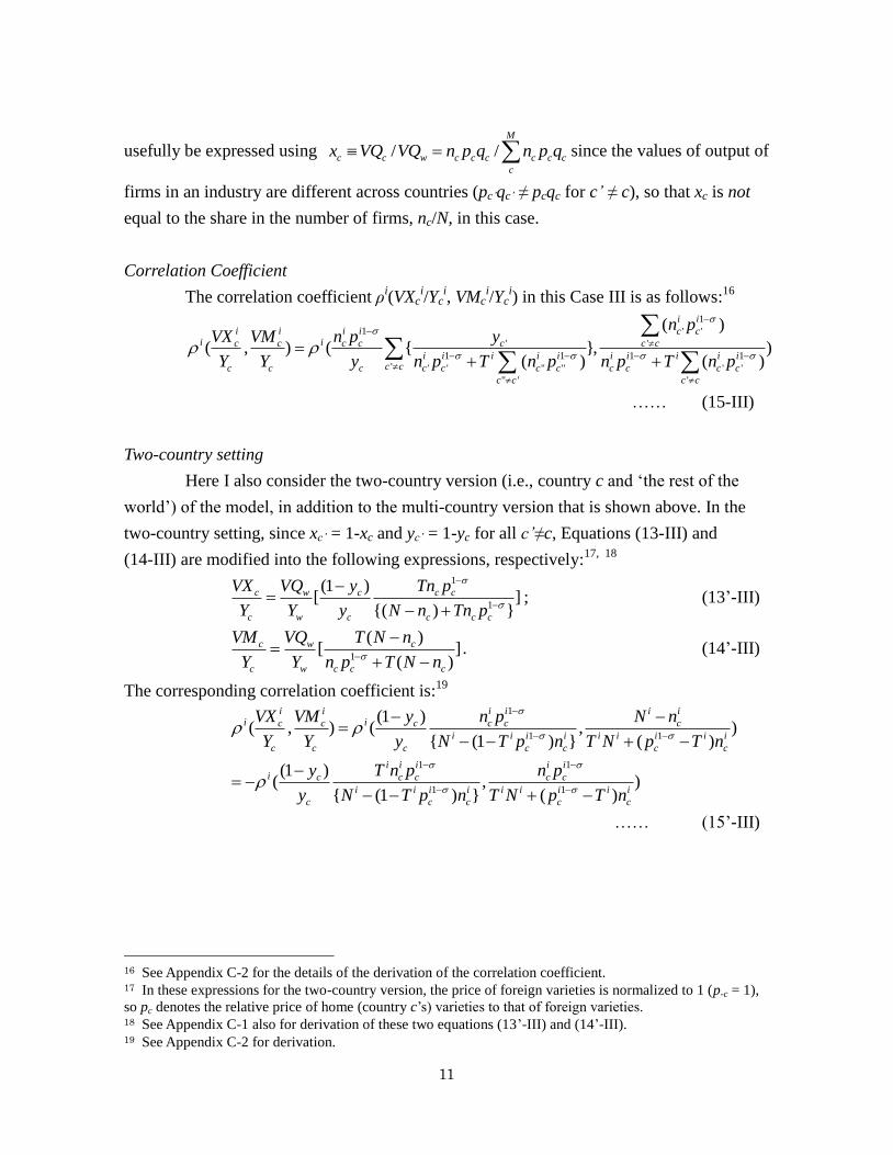
Correlation Coefficient

The correlation coefficient ρi(VXc

i/Yc

i, VMc

i/Yc

i) in this Case III is as follows:

16

1

1 ' '

' '

1 1 1 1' ' ' " " ' '

" ' '

( )

( , ) ( { }, )( ) ( )

i i

i i i i c ci ic c c c c c c

i i i i i i i i i ic cc c c c c c c c c c c

c c c c

n pVX VM n p y

Y Y y n p T n p n p T n p

…… (15-III)

Two-country setting

Here I also consider the two-country version (i.e., country c and ‘the rest of the

world’) of the model, in addition to the multi-country version that is shown above. In the

two-country setting, since xc’ = 1-xc and yc’ = 1-yc for all c’≠c, Equations (13-III) and

(14-III) are modified into the following expressions, respectively:17, 18

1

1

(1 )[ ]

{( ) }

c w c c c

c w c c c c

VX VQ y Tn p

Y Y y N n Tn p

; (13’-III)

1

( )[ ]

( )

c w c

c w c c c

VM VQ T N n

Y Y n p T N n

. (14’-III)

The corresponding correlation coefficient is:19

1

1 1

1 1

1 1

(1 )( , ) ( , )

{ (1 ) } ( )

(1 )( , )

{ (1 ) } ( )

i i i i i ii ic c c c c c

i i i i i i i i i

c c c c c c c

i i i i ii c c c c c

i i i i i i i i i

c c c c c

VX VM y n p N n

Y Y y N T p n T N p T n

y T n p n p

y N T p n T N p T n

…… (15’-III)

16 See Appendix C-2 for the details of the derivation of the correlation coefficient. 17 In these expressions for the two-country version, the price of foreign varieties is normalized to 1 (p-c = 1),

so pc denotes the relative price of home (country c’s) varieties to that of foreign varieties. 18 See Appendix C-1 also for derivation of these two equations (13’-III) and (14’-III). 19 See Appendix C-2 for derivation.

12

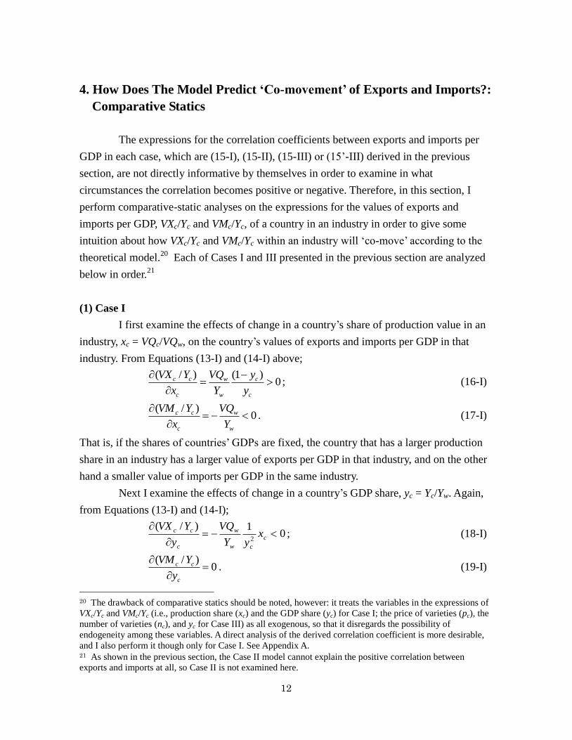
4. How Does The Model Predict ‘Co-movement’ of Exports and Imports?:

Comparative Statics

The expressions for the correlation coefficients between exports and imports per

GDP in each case, which are (15-I), (15-II), (15-III) or (15’-III) derived in the previous

section, are not directly informative by themselves in order to examine in what

circumstances the correlation becomes positive or negative. Therefore, in this section, I

perform comparative-static analyses on the expressions for the values of exports and

imports per GDP, VXc/Yc and VMc/Yc, of a country in an industry in order to give some

intuition about how VXc/Yc and VMc/Yc within an industry will ‘co-move’ according to the

theoretical model.20

Each of Cases I and III presented in the previous section are analyzed

below in order.21

(1) Case I

I first examine the effects of change in a country’s share of production value in an

industry, xc = VQc/VQw, on the country’s values of exports and imports per GDP in that

industry. From Equations (13-I) and (14-I) above;

( / ) (1 )0c c w c

c w c

VX Y VQ y

x Y y

; (16-I)

( / )0c c w

c w

VM Y VQ

x Y

. (17-I)

That is, if the shares of countries’ GDPs are fixed, the country that has a larger production

share in an industry has a larger value of exports per GDP in that industry, and on the other

hand a smaller value of imports per GDP in the same industry.

Next I examine the effects of change in a country’s GDP share, yc = Yc/Yw. Again,

from Equations (13-I) and (14-I);

01)/(

2

c

cw

w

c

cc xyY

VQ

y

YVX; (18-I)

( / )0c c

c

VM Y

y

. (19-I)

20 The drawback of comparative statics should be noted, however: it treats the variables in the expressions of

VXc/Yc and VMc/Yc (i.e., production share (xc) and the GDP share (yc) for Case I; the price of varieties (pc), the

number of varieties (nc), and yc for Case III) as all exogenous, so that it disregards the possibility of

endogeneity among these variables. A direct analysis of the derived correlation coefficient is more desirable,

and I also perform it though only for Case I. See Appendix A. 21 As shown in the previous section, the Case II model cannot explain the positive correlation between

exports and imports at all, so Case II is not examined here.

13

That is, if the sizes of the production of countries are all equal in an industry, the country

that has a larger GDP share in the world has a smaller value of exports per GDP in an

industry, but the values of imports per GDP do not vary across countries.

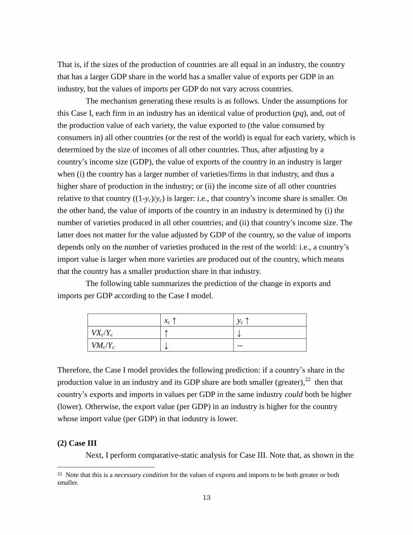
The mechanism generating these results is as follows. Under the assumptions for

this Case I, each firm in an industry has an identical value of production (pq), and, out of

the production value of each variety, the value exported to (the value consumed by

consumers in) all other countries (or the rest of the world) is equal for each variety, which is

determined by the size of incomes of all other countries. Thus, after adjusting by a

country’s income size (GDP), the value of exports of the country in an industry is larger

when (i) the country has a larger number of varieties/firms in that industry, and thus a

higher share of production in the industry; or (ii) the income size of all other countries

relative to that country ((1-yc)/yc) is larger: i.e., that country’s income share is smaller. On

the other hand, the value of imports of the country in an industry is determined by (i) the

number of varieties produced in all other countries; and (ii) that country’s income size. The

latter does not matter for the value adjusted by GDP of the country, so the value of imports

depends only on the number of varieties produced in the rest of the world: i.e., a country’s

import value is larger when more varieties are produced out of the country, which means

that the country has a smaller production share in that industry.

The following table summarizes the prediction of the change in exports and

imports per GDP according to the Case I model.

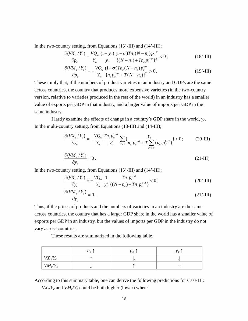
xc ↑ yc ↑

VXc/Yc ↑ ↓

VMc/Yc ↓ --

Therefore, the Case I model provides the following prediction: if a country’s share in the

production value in an industry and its GDP share are both smaller (greater),22

then that

country’s exports and imports in values per GDP in the same industry could both be higher

(lower). Otherwise, the export value (per GDP) in an industry is higher for the country

whose import value (per GDP) in that industry is lower.

(2) Case III

Next, I perform comparative-static analysis for Case III. Note that, as shown in the

22 Note that this is a necessary condition for the values of exports and imports to be both greater or both

smaller.

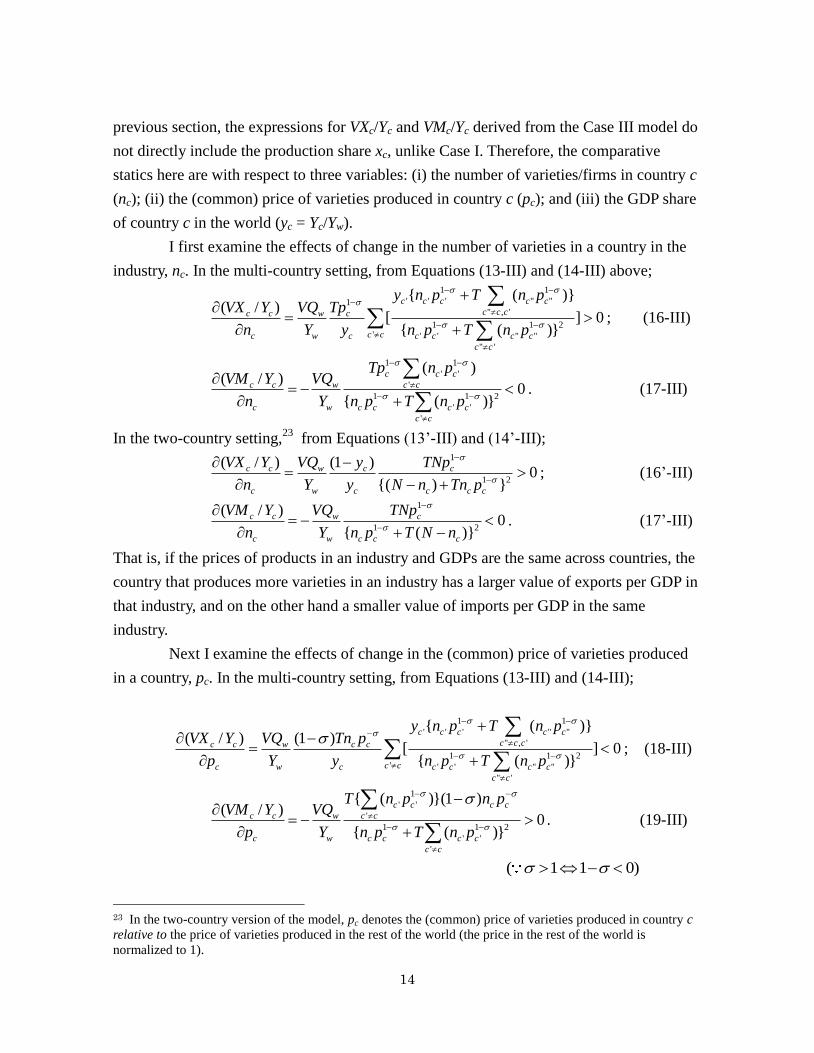
14

previous section, the expressions for VXc/Yc and VMc/Yc derived from the Case III model do

not directly include the production share xc, unlike Case I. Therefore, the comparative

statics here are with respect to three variables: (i) the number of varieties/firms in country c

(nc); (ii) the (common) price of varieties produced in country c (pc); and (iii) the GDP share

of country c in the world (yc = Yc/Yw).

I first examine the effects of change in the number of varieties in a country in the

industry, nc. In the multi-country setting, from Equations (13-III) and (14-III) above; 1 1

' ' ' " "1" , '

1 1 2' ' ' " "

" '

{ ( )}( / )

[ ] 0{ ( )}

c c c c c

c c cc c w c

c cc w c c c c c

c c

y n p T n pVX Y VQ Tp

n Y y n p T n p

; (16-III)

1 1

' '

'

1 1 2

' '

'

( )( / )

0{ ( )}

c c c

c c w c c

c w c c c c

c c

Tp n pVM Y VQ

n Y n p T n p

. (17-III)

In the two-country setting,23

from Equations (13’-III) and (14’-III); 1

1 2

( / ) (1 )0

{( ) }

c c w c c

c w c c c c

VX Y VQ y TNp

n Y y N n Tn p

; (16’-III)

1

1 2

( / )0

{ ( )}

c c w c

c w c c c

VM Y VQ TNp

n Y n p T N n

. (17’-III)

That is, if the prices of products in an industry and GDPs are the same across countries, the

country that produces more varieties in an industry has a larger value of exports per GDP in

that industry, and on the other hand a smaller value of imports per GDP in the same

industry.

Next I examine the effects of change in the (common) price of varieties produced

in a country, pc. In the multi-country setting, from Equations (13-III) and (14-III);

1 1

' ' ' " "

" , '

1 1 2' ' ' " "

" '

{ ( )}( / ) (1 )

[ ] 0{ ( )}

c c c c c

c c cc c w c c

c cc w c c c c c

c c

y n p T n pVX Y VQ Tn p

p Y y n p T n p

; (18-III)

1

' '

'

1 1 2

' '

'

{ ( )}(1 )( / )

0{ ( )}

c c c c

c c w c c

c w c c c c

c c

T n p n pVM Y VQ

p Y n p T n p

. (19-III)

( 1 1 0)

23 In the two-country version of the model, pc denotes the (common) price of varieties produced in country c

relative to the price of varieties produced in the rest of the world (the price in the rest of the world is

normalized to 1).

15

In the two-country setting, from Equations (13’-III) and (14’-III);

1 2

( / ) (1 ) (1 ) ( )0

{( ) }

c c w c c c c

c w c c c c

VX Y VQ y Tn N n p

p Y y N n Tn p

; (18’-III)

1 2

( / ) (1 ) ( )0

{ ( )}

c c w c c c

c w c c c

VM Y VQ Tn N n p

p Y n p T N n

. (19’-III)

These imply that, if the numbers of product varieties in an industry and GDPs are the same

across countries, the country that produces more expensive varieties (in the two-country

version, relative to varieties produced in the rest of the world) in an industry has a smaller

value of exports per GDP in that industry, and a larger value of imports per GDP in the

same industry.

I lastly examine the effects of change in a country’s GDP share in the world, yc.

In the multi-country setting, from Equations (13-III) and (14-III);

1

'

2 1 1' ' ' " "

" '

( / ){ } 0

( )

c c w c c c

c cc w c c c c c

c c

VX Y VQ Tn p y

y Y y n p T n p

; (20-III)

( / )0c c

c

VM Y

y

. (21-III)

In the two-country setting, from Equations (13’-III) and (14’-III); 1

2 1

( / ) 10

{( ) }

c c w c c

c w c c c c

VX Y VQ Tn p

y Y y N n Tn p

; (20’-III)

( / )0c c

c

VM Y

y

. (21’-III)

Thus, if the prices of products and the numbers of varieties in an industry are the same

across countries, the country that has a larger GDP share in the world has a smaller value of

exports per GDP in an industry, but the values of imports per GDP in the industry do not

vary across countries.

These results are summarized in the following table.

nc ↑ pc ↑ yc ↑

VXc/Yc ↑ ↓ ↓

VMc/Yc ↓ ↑ --

According to this summary table, one can derive the following predictions for Case III:

VXc/Yc and VMc/Yc could be both higher (lower) when:

16

(i) nc is lower (higher) as yc is lower (higher);

(ii) pc is higher (lower) as yc is lower (higher); or

(iii) pc is higher (lower) and nc is lower (higher) as yc is lower (higher).

Can production share (xc) be a ‘predictor’ in Case III, too?

As shown above, in Case III, VXc/Yc and VMc/Yc depend on the three variables: pc,

nc, and yc, while they depend only on the two variables, xc and yc, in Case I. However,

prices (pc’s) and the numbers of firms/varieties (nc’s) are in general much more difficult to

observe in data24

than countries’ shares of production in an industry (xc = VQc/VQw). Then,

isn’t it possible to give similar predictions of the ‘co-movement’ of VXc/Yc and VMc/Yc only

from the observable variables xc and yc without having the information on prices and the

numbers of varieties? My answer is YES: it is possible. The reason is as follows:25

Using the technique of total differentiation, the following conditions are derived for a

change in the value of a country’s total production in an industry, VQc:

0c c Q cdVQ dn B dp

0c c Q cdVQ dn B dp ;

where /

( )/

c cQ

c c

VQ pB

VQ n

.

In the same manner, for the values of exports and imports per GDP;

( ) ( )0 ( )cc X c

c

VXd dn B dp

Y where

( / ) /( )

( / ) /

c c cX

c c c

VX Y pB

VX Y n

;

( ) ( )0 ( )cc M c

c

VMd dn B dp

Y where

( / ) /( )

( / ) /

c c cM

c c c

VM Y pB

VM Y n

.

However, it is derived that:

Q X MB B B (1 ) / 0c cn p (for the multi-country version)

(1 ) ( ) / 0c c cn N n Np (for the two-country version)

In addition, ( ) ( )c csign dVQ sign dx 26.

24 The price information may be observable if data are detailed enough. However, the number of firms (nc) is

generally unobservable because this variable comes from the assumptions of the model, which does not mean

the real number of firms. 25 For the technical details of the following part, see Appendix C-4. 26 See Appendix C-4.

17

Therefore, one can conclude that, if countries’ shares of GDP (yc’s) are fixed;

0 ( / ) 0 ( / ) 0c c c c cdx d VX Y d VM Y

0 ( / ) 0 ( / ) 0c c c c cdx d VX Y d VM Y

That is, the country that has a larger production share in an industry has a larger value of

exports per GDP, and a smaller value of imports per GDP.

One can thus give a prediction of the ‘co-movement’ of VXc/Yc and VMc/Yc from

the two observables xc and yc also in this Case III such as in the table below:27

xc ↑ yc ↑

VXc/Yc ↑ ↓

VMc/Yc ↓ --

This prediction of the model is thus the same as that in Case I: if a country’s share in the

production value in an industry and its GDP share are both smaller (greater)28

, then that

country’s exports and imports in values per GDP in the same industry could both be higher

(lower). Otherwise, the export value (per GDP) in an industry is higher for the country

whose import value (per GDP) in that industry is lower.

5. Data Analysis of Correlation (Case I only)

Previous sections have shown that, according to the model, the exports and imports

in an industry per GDP, VXci/Yc

i and VMc

i/Yc

i, and their ‘co-movement’ can be predicted by

‘predictors,’ which are each country’s share of production in that industry (xc) and its share

of GDP (yc) for Case I; the (common) price of each country’s product varieties in an

industry (pc), the number of varieties in each country (nc), and yc for Case III. In this section,

I use data to examine how close the predicted measure of the correlation coefficient

between VXci/Yc

i and VMc

i/Yc

i (ρ

i(VXc

i/Yc

i, VMc

i/Yc

i)) based on these ‘predictors’ is to the

direct measure of the correlation coefficient. This is a test of the extent to which the

standard model (and its variation) can explain the observed positive correlation between

exports and imports within the same industry. Cross-country data on production and

27 Note that, however, for an accurate analysis of the correlation coefficients with data, one still needs the

variables pc and nc rather than xc. I discuss this in the next section and propose a procedure for a data analysis

in Appendix B. 28 See Footnote 22.

18

international trade in manufacturing industries and GDP are employed.

Here I examine only the Case I model, for which all the necessary ‘predictors’ are

available in the data, but not the Case III model that requires the prices and the numbers of

varieties as ‘predictors’, both of which are not directly observable in the data. Instead, in

Appendix B, I propose a possible procedure for a data analysis of Case III without having

these unobserved variables.

In the following parts of this section, I first re-present the expressions for the

correlation coefficient for each of Cases I and III,29

then describe the data, and finally show

the results for Case I.

(1) Predicted Measure of Correlation Coefficient

Let us recall the following expression for the coefficient of correlation across

countries, ρi(VXc

i/Yc

i, VMc

i/Yc

i), which has been derived in Section 3 for each of Case I and

Case III.

Case I:

(15-I): 1 1

( , ) ( ,1 ) ( , )i i

i i i i i i ic c c cc c c c

c c c c

VX VM y yx x x x

Y Y y y

.

Case III:

For the multi-country version, (15-III): 1

1 ' '

' '

1 1 1 1' ' ' " " ' '

" ' '

( )

( , ) ( { }, )( ) ( )

i i

i i i i c ci ic c c c c c c

i i i i i i i i i ic cc c c c c c c c c c c

c c c c

n pVX VM n p y

Y Y y n p T n p n p T n p

For the two-country version, (15’-III): 1

1 1

1 1

1 1

(1 )( , ) ( , )

{ (1 ) } ( )

(1 )( , )

{ (1 ) } ( )

i i i i i ii ic c c c c c

i i i i i i i i i

c c c c c c c

i i i i ii c c c c c

i i i i i i i i i

c c c c c

VX VM y n p N n

Y Y y N T p n T N p T n

y T n p n p

y N T p n T N p T n

The right-hand side of each expression above is the predicted measure of the correlation

coefficient. That is, if the model correctly predicts countries’ export and import values per

GDP, the cross-country correlation coefficients calculated by the formula above showed

29 Case II has been omitted for further examination, as mentioned in Section 3.

19

equal the actual values of ρi(VXc

i/Yc

i, VMc

i/Yc

i). Note, however, that the predicted measure

of the correlation coefficient for Case III requires the price information for pci, which is not

available in the data used for this paper, as well as the number of product varieties, nci,

which is unobservable in reality.30

On the other hand, the Case I model requires only the

data on countries’ GDPs and production, both of which are available in the dataset

described below.

(2) Data

The data I employ for this paper contain the variables of production, exports,

imports, and GDP of various countries. The data on production are from UNIDO (2003).

The values of the (gross) output in manufacturing industries in U.S. dollars (USD) were

selected. The data on exports and imports are from Feenstra, Lipsey, and Bowen (1997) and

Feenstra (2000). The original datasets provide the values of exports and imports for each

bilateral pair, and I summed up these bilateral trade values for each origin country (for

exports) and for each destination country (for imports). The trade data are in thousands of

USD. The GDP data in current USD were taken from the World Bank (2002).

There is an issue concerning the industry classifications employed by the data

sources. UNIDO’s production dataset categorizes manufacturing industries according to the

International Standard Industrial Classification (ISIC: Revision 2) at the 3-digit level, while

Feenstra et al.’s trade data are categorized by the Standard International Trade

Classification (SITC: Revision 2) at the 4-digit level. I transformed the original trade data

into ISIC utilizing the concordance information provided by OECD, which is made

available on the web page of Jon Haveman’s Industry Concordances.31

I selected the data for the years of 1970, 1975, 1980, 1985, 1990, and 1995.32

Since availability of the data is different across industries, countries and years, I used for

each industry only the countries for which all the variables of production, exports, imports,

and GDP are available in order to calculate the across-country correlation coefficient for

each industry in each year.33

The sample size thus varies from 22 countries to 77 countries

30 See Footnote 24. 31 URL: http://www.macalester.edu/research/economics/PAGE/HAVEMAN/Trade.Resources/

tradeconcordances.html 32 UNIDO’s dataset on production covers the period of 1963-2001, Feenstra et al.’s (1997) trade data covers

1970-1992, which is supplemented by Feenstra (2000) through the year of 1997. The GDP data from the

World Bank (2002) covers the period of 1960-2000. 33 To obtain xc

i = VQc

i/VQw

i and yc = Yc/Yw, I needed to calculate the world total value of production in each

industry (i i

W ccVQ VQ ) and world GDP ( W cc

Y Y ). For each summation I include the countries for

which the figure to be summed (VQci or Yc) is available even if the countries are not included in the sample for

20

by industry and year. Table 2 shows the number of countries included in the sample for

each industry in each year.

(3) Result (for Case I)

The actual ρi(VXc

i/Yc

i, VMc

i/Yc

i) and the correlation coefficient predicted by the

Case I model are compared for each industry and each period in Table 3. Although the

actual correlations are significantly positive in many industries and years, the correlations

predicted by the model are mostly small or negative (see Figure 2). Although there are

several industries in which the predicted correlations are fairly close to, or even greater than,

the actual, the model predicts much lower values for the correlation coefficients than the

actual coefficients in most industries (see Figure 3). That is, at least in its Case I version,

the model cannot explain the strong positive correlations found in the data.

In Section 4, I used comparative statics to show that the necessary condition for

VXci/Yc

i and VMc

i/Yc

i to ‘move together’ (i.e., both be higher or lower) is that a country with

a larger (smaller) production share (xci) has a larger (smaller) GDP share (yc). Indeed, as

shown in Table 4, in the data xci and yc are almost perfectly correlated: that is, in any

industry, a country with a larger GDP share almost always has a larger production share.34

However, the more direct term that is included in the expression of VXci/Yc

i derived from

the model is (1-yc)/yc: that is, GDP of ‘the rest of the world’ relative to a country’s own GDP,

rather than the country’s own GDP itself. In other words, a country’s exports and imports

(in values per GDP) become both smaller (greater) when the country has a larger (smaller)

production share but the GDPs of the other countries are smaller (greater) relative to that

country’s. This mechanism also applies to Case III. Therefore, I also list the correlations

between xci and (1-yc)/yc in Table 4. The signs of the correlations are indeed all negative, as

the model requires for positive correlations between exports and imports, but the values are

small: they are all between -0.1 and -0.3. It might thus be necessary to have more strongly

negative correlations between xci and (1-yc)/yc to predict the strongly positive correlations

between exports and imports such as found in the data. This may be so also in Case III.35

each industry/year. Therefore, the sum of xc

i’s and that of yc’s are not necessarily equal to one. (However, I

should note that, when I include only the countries in the sample, in order for the sum of xci’s and that of yc’s

to be one, the results presented below do not change.) 34 Moreover, the values of xc

i and yc are almost equal to each other for many countries in most industries and

years: the two variables are almost on a ’45-degree line’. 35 Appendix B also presents the result of the data analysis for Case III by the proposed ‘indirect’ method.

21

6. Concluding Discussion

In this paper I employed the monopolistic competition model of intra-industry

trade that is widely used in the trade literature, first with the assumptions of free trade and

identical production technologies in an industry; and then with the more relaxed

assumptions allowing existence of transport costs and price asymmetry within an industry

across countries, in order to see whether such a model can explain the positive correlation

between countries’ exports and imports in values per GDP within one industry that is

observed in the data for most manufacturing industries. The theoretical model tells, in both

its restricted and relaxed versions, that a country’s exports and imports in value per GDP in

an industry could both be higher (lower) if the country’s share of the production value in

that industry in the world and its GDP share in the world are both smaller (greater);

otherwise the export value per GDP in an industry is higher for the country whose import

value per GDP in that industry is lower. However, the cross-country correlations between

exports and imports predicted by the model from the data on manufacturing production and

GDP of various countries showed that the model cannot explain, at least in its restricted

form, such positive correlations between exports and imports as observed in the data, while

the correlations between the countries’ production shares and GDPs are almost equal to one

in most of the industries. For the relaxed case allowing iceberg transport cost and price

asymmetry across countries, a data analysis is not straightforward because of data

limitation, but inferring from the result of the comparative statics in Section 4, this relaxing

of the assumptions may not be enough to make the conventional model capable of

explaining the fact.36

What can explain the positive correlation between exports and imports within the

same industry? What can be an alternative model to the conventional monopolistic

competition model of trade? Harrigan (1994) pointed out that the “love of varieties”

assumption for the consumer’s preference, which is represented by a CES utility function

over all available varieties, is the driving force of intra-industry trade in this type of model,

and similar models with the preference assumption such as Deardorff and Stern (1986) also

generate intra-industry trade. In fact, the analysis in this paper relies on the demand side of

the conventional model, so that the result here implies that the assumption on the

consumers’ preferences may need to be reconsidered. Or, being a little less ambitious, the

model with further-relaxed assumptions on transport costs could explain the fact. Hummels

36 Indeed, as shown in Appendix B, the data analysis performed according to the proposed ‘indirect’ method

concludes that the model does not explain the positive correlation well even under the relaxed assumptions.

22

and Levinsohn (1995) presented evidence of a significant effect of distance between two

countries on the volume of bilateral intra-industry trade. Haveman and Hummels (2004)

pointed out that countries may be choosing their sources of import (or trading partners)

taking account of bilateral transport costs.37

Therefore, the monopolistic competition

model might be able to explain the positive correlation between exports and imports if it

incorporates transport cost that differs for each pair of countries. These could be directions

for future research.

A considerable amount of research has been conducted on the volume of

intra-industry trade, including a series of studies on the gravity equation. All of them,

however, focused on the total volume of trade without paying much attention to the

direction of the trade: how much is exported or imported. By pointing out the ‘fact’ of the

positive correlation between exports and imports, which is inconsistent with conventional

models based only on comparative advantage, and which may be puzzling according to the

conventional monopolistic competition model, this study presents a new issue to be

considered when examining what is a plausible theory of international trade.

37 It should be noted that Haveman and Hummels discussed this in the context of the model with imperfect

specialization of countries’ production, while the model analyzed in this paper features countries’ perfect

specialization in certain varieties of a good.

23

Appendix A

Section 4 has performed comparative-static analysis to provide some intuition on the

‘co-movement’ of countries’ export and import values per GDP within the same industry

(VXci/Yc and VMc

i/Yc), but it does not necessarily directly tell what the correlation

coefficient of these two variables will be in various circumstances. In this appendix, I

present a direct examination of the correlation coefficient. Specifically, limiting the analysis

to the Case I model and focusing on five potential circumstances on the patterns of

countries production sizes and GDPs, I show whether the model predicts the correlation to

be positive or negative in each circumstance.38

Preliminaries

Recall Equation (15-I):

1 1( , ) ( ,1 ) ( , )

i ii i i i i i ic c c c

c c c c

c c c c

VX VM y yx x x x

Y Y y y

.

Then;

1( , ) ( )0 ( , ) ( )0

i ii i i ic c c

c c

c c c

VX VM yx x

Y Y y

1( , ) ( )0i ic

c c

c

yCov x x

y

( ) ( ) ( , )i

i icc c

c

xVar x Cov x

y . …… (*)

Therefore, in the following parts of this appendix, with which inequality (*) holds is

examined in each case.

Five Potential Cases and Expected Correlations

Case (i): yc is the same for all countries

The first case to be examined is when all countries are in an equal size: i.e., the

countries all have the same GDP regardless of their industrial production compositions. In

this case, each country’s share of GDP in the world, yc, is equal to 1/N where N(≥2) is the

number of countries in the world. Therefore;

38 The detailed derivation or the proof of the expressions or (in)equalities that appear in this appendix are

suppressed to avoid lengthiness, but these can be provided by the author upon request.

24

( , ) ( , ) ( ) ( )i

i i i i icc c c c c

c

xCov x Cov Nx x N Var x Var x

y ;

and thus the model predicts the correlation between export and import per GDP to be

negative.

More specifically, in this case, the correlation coefficient is:

1( , ) ( , ) (( 1) , ) 1

i ii i i i i i ic c c

c c c c

c c c

VX VM yx x N x x

Y Y y

:

that is, a perfect negative correlation is predicted.

Case (ii): xci is constant for all countries

The next case is when, in a certain industry, all the countries produce the same

value: i.e., the countries’ production sizes are all equal, regardless of the sizes of their

economies or GDPs. In this case, each country’s share of production in that industry in the

world, xci, is equal to 1/N. Therefore;

1 1( ) (1/ ) ( , ) ( , ) 0

ii icc c

c c

xVar x Var N Cov x Cov

y N y N

.

That is, in this case, the correlation coefficient is undefined, while the covariance between

exports and imports per GDP becomes zero.

It is natural to think that the larger a country’s GDP is, the larger the country’s

production size in an industry is.39

The following three cases are all in such a circumstance.

Case (iii): xci = yc

This case is when a country’s share of production in an industry equals its GDP

share: i.e., the production size of each country in an industry is proportional to the country’s

GDP. In this case;

( , ) (1, ) 0 ( )i

i i icc c c

c

xCov x Cov x Var x

y ;

and thus the correlation between export and import per GDP is expected to be positive.

More specifically, the correlation coefficient in this case is:

1( , ) ( , ) (1 , ) 1

i ii i i i ic c c

c c c c

c c c

VX VM yx x y y

Y Y y

:

that is, exports and imports are predicted to be perfectly correlated.

39 Indeed, as shown in Table 4, countries’ production shares and GDP shares are almost perfectly correlated

in almost all manufacturing industries.

25

Case (iv): xci = (1-a)/N + a∙yc; 0<a<1

This case implies that countries’ GDPs are more diversified than their sizes of

production in an industry, or in other words, the degree of countries’ specialization in that

industry is not very large.40

In this case;

(1 ) 1( , ) ( , ) 0 ( )

ii icc c c

c c

x a aCov x Cov y Var x

y N y

;

and thus the correlation between export and import per GDP is expected to be positive.

Case (v): yc = (1-a)/N + a∙xci; 0<a<1

This case contrasts with Case (iv) above: that is, this case implies that countries’

sizes of production in an industry are more diversified than their GDPs. In other words, the

degree of countries’ specialization in that industry is very large.41

In this case;

2

1( ) ( )

(1 ) 1( , ) ( , )

i

c c

iicc c

c c

Var x Var ya

x aCov x Cov y

y N a y

In fact, the former value becomes greater than the latter value ( ( ) ( / , )i i i

c c c cVar x Cov x y x )

only when the value of a is very close to one. That is, in this case, the correlation between

export and import per GDP can be positive when the production of each country in an

industry is almost proportional to its GDP, but the correlation is predicted to be negative

otherwise.42

Summary: When Will Correlation Be Positive?

By summarizing the five cases examined above, the following conclusion is

derived:

The Case I model predicts that the correlation between countries’ export and import

values per GDP within the same industry will be positive when the following

40 Being more accurate, this is a special linear case of such a circumstance. Note that, in this case, it holds

that 1N Ni i

c cc cx y .

41 This is a special linear case of such a circumstance. Note that, also in this case, it holds that

1N Ni i

c cc cx y .

42 In fact, in the limit as N rises to infinity, any a such that 0<a<1 cannot generate a positive correlation,

which means that the correlation is expected to be always negative.

26

conditions are all satisfied: (i) countries vary both in their shares of production in

the industry and in their shares of GDP; (ii) the larger a country’s GDP, the larger

the country’s production share in the industry; and (iii) a country’s production share

is almost equal to its GDP share, or the dispersion of countries’ GDP shares is

greater than that of their production shares (i.e., countries are not very specialized in

production).

27

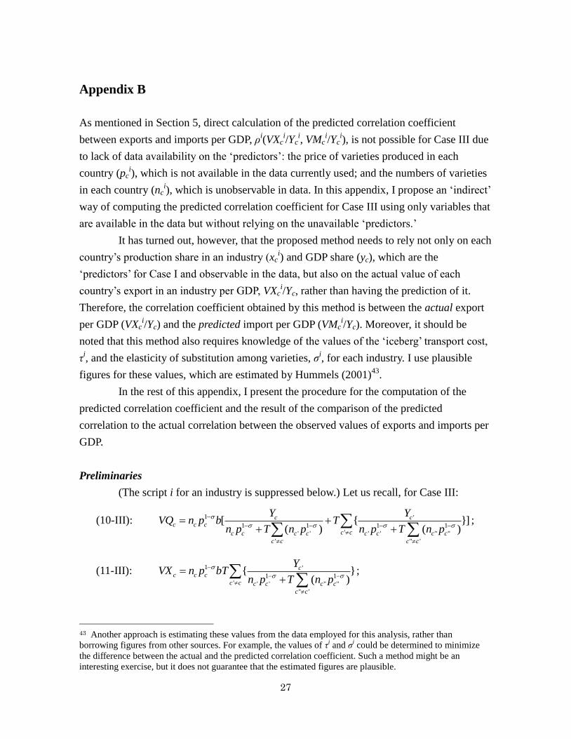
Appendix B

As mentioned in Section 5, direct calculation of the predicted correlation coefficient

between exports and imports per GDP, ρi(VXc

i/Yc

i, VMc

i/Yc

i), is not possible for Case III due

to lack of data availability on the ‘predictors’: the price of varieties produced in each

country (pci), which is not available in the data currently used; and the numbers of varieties

in each country (nci), which is unobservable in data. In this appendix, I propose an ‘indirect’

way of computing the predicted correlation coefficient for Case III using only variables that

are available in the data but without relying on the unavailable ‘predictors.’

It has turned out, however, that the proposed method needs to rely not only on each

country’s production share in an industry (xci) and GDP share (yc), which are the

‘predictors’ for Case I and observable in the data, but also on the actual value of each

country’s export in an industry per GDP, VXci/Yc, rather than having the prediction of it.

Therefore, the correlation coefficient obtained by this method is between the actual export

per GDP (VXci/Yc) and the predicted import per GDP (VMc

i/Yc). Moreover, it should be

noted that this method also requires knowledge of the values of the ‘iceberg’ transport cost,

τi, and the elasticity of substitution among varieties, σ

i, for each industry. I use plausible

figures for these values, which are estimated by Hummels (2001)43

.

In the rest of this appendix, I present the procedure for the computation of the

predicted correlation coefficient and the result of the comparison of the predicted

correlation to the actual correlation between the observed values of exports and imports per

GDP.

Preliminaries

(The script i for an industry is suppressed below.) Let us recall, for Case III:

(10-III): 1 '

1 1 1 1'' ' ' ' " "

' " '

[ { }]( ) ( )

c cc c c

c cc c c c c c c c

c c c c

Y YVQ n p b T

n p T n p n p T n p

;

(11-III): 1 '

1 1' ' ' " "

" '

{ }( )

cc c c

c c c c c c

c c

YVX n p bT

n p T n p

;

43 Another approach is estimating these values from the data employed for this analysis, rather than

borrowing figures from other sources. For example, the values of τi and σ

i could be determined to minimize

the difference between the actual and the predicted correlation coefficient. Such a method might be an

interesting exercise, but it does not guarantee that the estimated figures are plausible.

28

(12-III):

1

' '

'

1 1

' '

'

( )

( )

c c c

c cc

c c c c

c c

bY T n p

VMn p T n p

.

Define:

1

c c cz n p ;

'

'

1/( )c c c

c c

w z T z

.

Then, Equations (10-III) through (12-III) above can be expressed as follows:

' '

'

[ ]c c c c c c

c c

VQ z b w Y T w Y

; (i)

' '

'

c c c c c c c c

c c

VX z bT w Y VQ z bw Y

; (ii)

'

'

c c c c

c c

VM w Y bT z

. (iii)

Equation (ii) implies:

c cc c c c c c

c c

VQ VXz bw Y VQ VX w

bz Y

. (ii)’

Then, by the definition of wc, the equation below follows:

'

'

(1/ ) /( )c c c c c c c

c c

w z T z bz Y VQ VX

. (iv)

Equation (iv) holds for any country c. Also note that )('

'

'

' c

c

c

cc

c zzTzT

. Thus,

considering Equation (iv) for two countries c and c’ (c ≠ c’), and subtracting one from

another on both sides, yields:

' ''

' '

(1 )( ) ( )c c c cc c

c c c c

z Y z YT z z b

VQ VX VQ VX

.

Define /( )c c c cR Y VQ VX . Then, since 10 1T , the equation above implies:

' '{1 } {1 }1 1

c c c c

b bR z R z

T T

.

Here, define the “benchmark” country c = 0 such that 1

0 0 0 1z n p . Then, the equation

above can be expressed as follows:

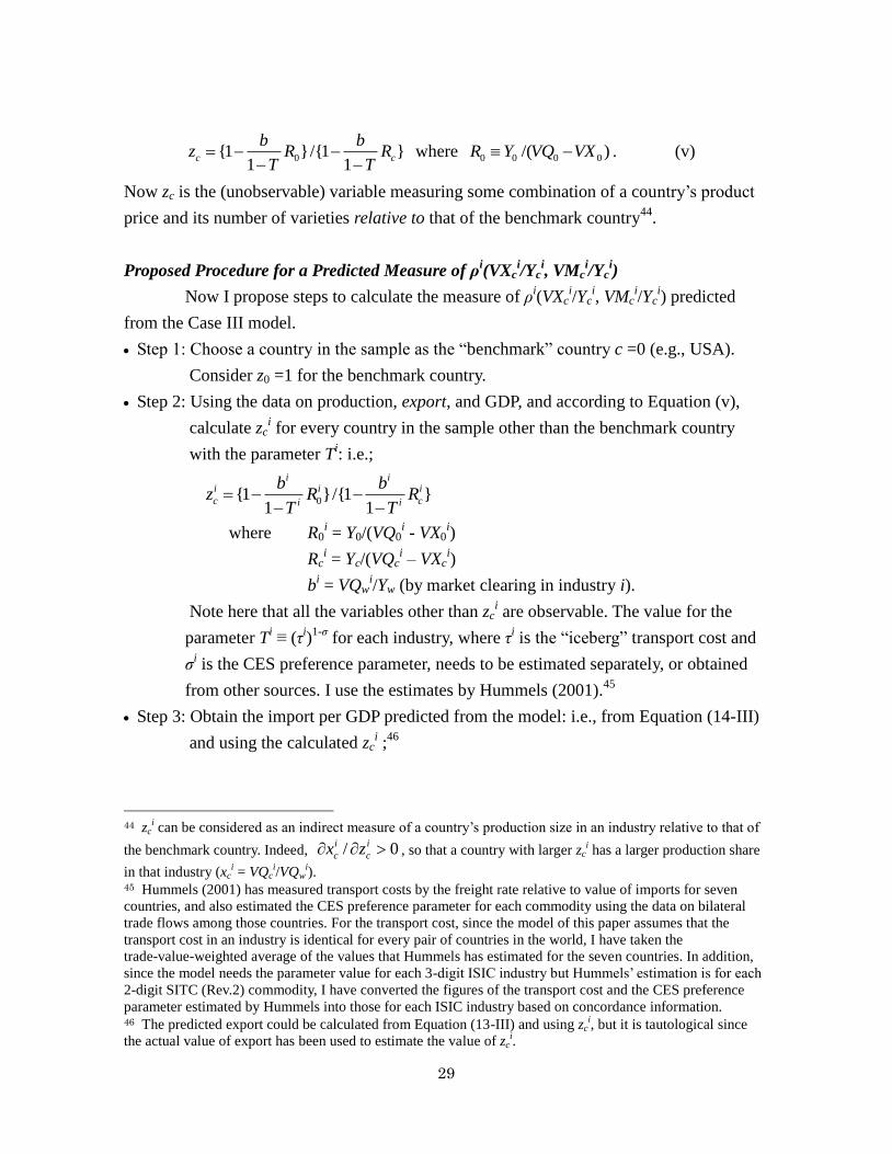
29

0{1 }/{1 }1 1

c c

b bz R R

T T

where 0 0 0 0/( )R Y VQ VX . (v)

Now zc is the (unobservable) variable measuring some combination of a country’s product

price and its number of varieties relative to that of the benchmark country44

.

Proposed Procedure for a Predicted Measure of ρi(VXc

i/Yc

i, VMc

i/Yc

i)

Now I propose steps to calculate the measure of ρi(VXc

i/Yc

i, VMc

i/Yc

i) predicted

from the Case III model.

Step 1: Choose a country in the sample as the “benchmark” country c =0 (e.g., USA).

Consider z0 =1 for the benchmark country.

Step 2: Using the data on production, export, and GDP, and according to Equation (v),

calculate zci for every country in the sample other than the benchmark country

with the parameter Ti: i.e.;

0{1 }/{1 }1 1

i ii i i

c ci i

b bz R R

T T

where R0i = Y0/(VQ0

i - VX0

i)

Rci = Yc/(VQc

i – VXc

i)

bi = VQw

i/Yw (by market clearing in industry i).

Note here that all the variables other than zci are observable. The value for the

parameter Ti ≡ (τ

i)1-σ

for each industry, where τi is the “iceberg” transport cost and

σi is the CES preference parameter, needs to be estimated separately, or obtained

from other sources. I use the estimates by Hummels (2001).45

Step 3: Obtain the import per GDP predicted from the model: i.e., from Equation (14-III)

and using the calculated zci ;

46

44 zc

i can be considered as an indirect measure of a country’s production size in an industry relative to that of

the benchmark country. Indeed, / 0i i

c cx z , so that a country with larger zci has a larger production share

in that industry (xci = VQc

i/VQw

i).

45 Hummels (2001) has measured transport costs by the freight rate relative to value of imports for seven

countries, and also estimated the CES preference parameter for each commodity using the data on bilateral

trade flows among those countries. For the transport cost, since the model of this paper assumes that the

transport cost in an industry is identical for every pair of countries in the world, I have taken the

trade-value-weighted average of the values that Hummels has estimated for the seven countries. In addition,

since the model needs the parameter value for each 3-digit ISIC industry but Hummels’ estimation is for each

2-digit SITC (Rev.2) commodity, I have converted the figures of the transport cost and the CES preference

parameter estimated by Hummels into those for each ISIC industry based on concordance information. 46 The predicted export could be calculated from Equation (13-III) and using zc

i, but it is tautological since

the actual value of export has been used to estimate the value of zci.

30

1

' '

'

1 1

' '

'

( )

[ ]( )

i

i i

i i

i i c c

c w c c

i i ic w c c c c

c c

T n pVM VQ

Y Y n p T n p

.

Step 4: Calculate the correlation coefficient, ρi(VXc

i/Yc

i, VMc

i/Yc

i), using the actual value

of VXci/Yc

i and the estimated value of VMc

i/Yc

i obtained in Step 3 above.

Result

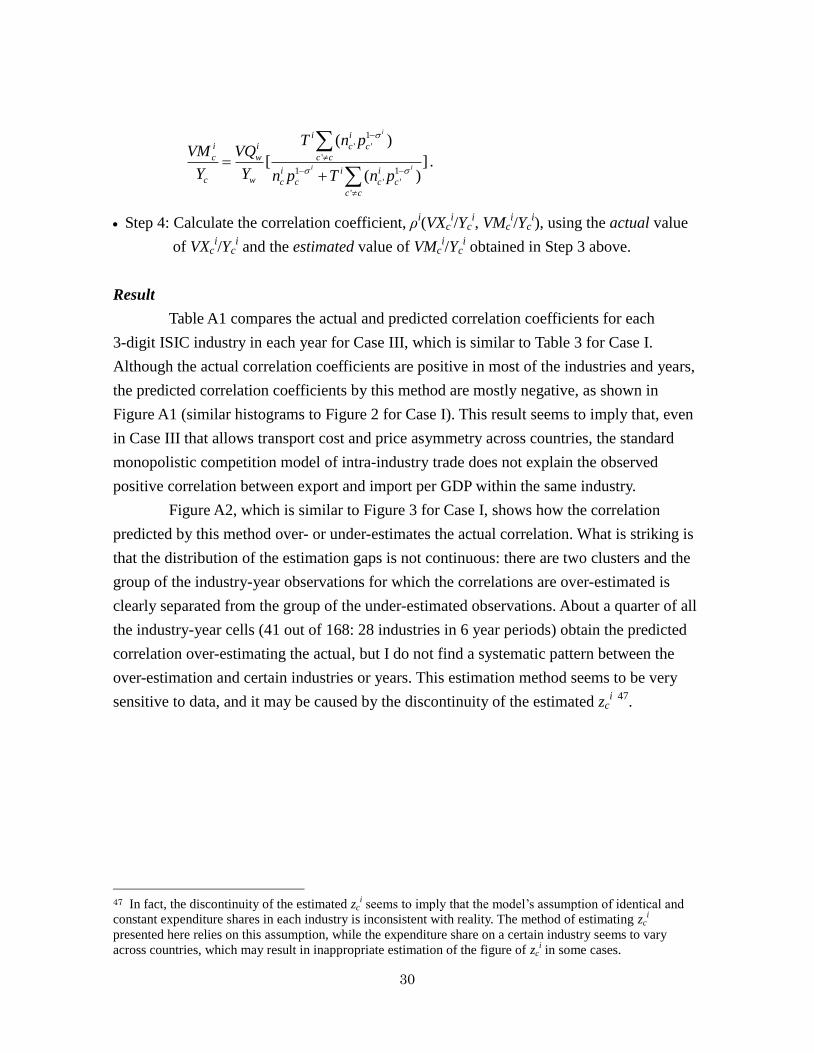
Table A1 compares the actual and predicted correlation coefficients for each

3-digit ISIC industry in each year for Case III, which is similar to Table 3 for Case I.

Although the actual correlation coefficients are positive in most of the industries and years,

the predicted correlation coefficients by this method are mostly negative, as shown in

Figure A1 (similar histograms to Figure 2 for Case I). This result seems to imply that, even

in Case III that allows transport cost and price asymmetry across countries, the standard

monopolistic competition model of intra-industry trade does not explain the observed

positive correlation between export and import per GDP within the same industry.

Figure A2, which is similar to Figure 3 for Case I, shows how the correlation

predicted by this method over- or under-estimates the actual correlation. What is striking is

that the distribution of the estimation gaps is not continuous: there are two clusters and the

group of the industry-year observations for which the correlations are over-estimated is

clearly separated from the group of the under-estimated observations. About a quarter of all

the industry-year cells (41 out of 168: 28 industries in 6 year periods) obtain the predicted

correlation over-estimating the actual, but I do not find a systematic pattern between the

over-estimation and certain industries or years. This estimation method seems to be very

sensitive to data, and it may be caused by the discontinuity of the estimated zci 47

.

47 In fact, the discontinuity of the estimated zc

i seems to imply that the model’s assumption of identical and

constant expenditure shares in each industry is inconsistent with reality. The method of estimating zci

presented here relies on this assumption, while the expenditure share on a certain industry seems to vary

across countries, which may result in inappropriate estimation of the figure of zci in some cases.

31

References

Deardorff, Alan V. (1980), “The General Validity of the Law of Comparative Advantage”,

Journal of Political Economy, 88(5), pp.941-957.

Deardorff, Alan V., and Stern, Robert M. (1986), The Michigan Model of World Production

and Trade, MIT Press, Cambridge, MA.

Feenstra, Robert C.; Lipsey, Robert E., and Bowen, Harry P. (1997), “World Trade Flows,

1970-1992, with Production and Tariff Data”, NBER Working Paper No.5910.

Feenstra, Robert C. (2000), “World Trade Flows, 1980-1997”, Center for International Data,

Institute of Governmental Affairs, University of California, Davis.

Finger, J. M. (1975), “Trade Overlap and Intra-Industry Trade”, Economic Inquiry, 13(4),

pp.581-589.

Harrigan, James (1994), “Scale Economies and The Volume of Trade”, Review of

Economics and Statistics, 76(2), pp.321-328.

Haveman, Jon, and Hummels, David (2004), “Alternative Hypotheses and The Volume of

Trade: The Gravity Equation and The Extent of Specialization”, Canadian Journal of

Economics, 37(1), pp.199-218.

Helpman, Elhanan, and Krugman, Paul R. (1985), Market Structure and Foreign Trade,

MIT Press, Cambridge, MA.

Hummels, David (2001), “Toward a Geography of Trade Costs”, manuscript.

Hummels, David, and Levinsohn, James (1995), “Monopolistic Competition and

International Trade: Reconsidering The Evidence”, Quarterly Journal of Economics, 110,

pp.799-836.

Krugman, Paul R. (1979), “Increasing Returns, Monopolistic Competition, and

International Trade”, Journal of International Economics, 9, pp.469-479.

32

Krugman, Paul R. (1980), “Scale Economies, Product Differentiation, and the Patterns of

Trade”, American Economic Review, 70(5), pp.950-959.

Romalis, John (2004), “Factor Proportions and the Structure of Commodity Trade”,

American Economic Review, 94(1), pp.67-97.

UNIDO: United Nations Industrial Development Organization (2003), Industrial Statistics

Database at the 3-digit level of ISIC Code (Rev.2) (INDSTAT3 2003 ISIC Rev.2).

World Bank (2002), World Development Indicators 2002.

33

Table 1: Correlations between Volumes of Exports and Imports per GDP across Countries

Industry*

Year

1970 1975 1980 1985 1990 1995

311 (Food products) .183 .304 .085 .202 .314 .184

313 (Beverages) .646 .041 .058 .384 .381 .269

314 (Tobacco) .431 .498 .513 .670 .248 .185

321 (Textiles) .084 .494 .424 .123 .131 .412

322 (Wearing apparel) .432 .208 .375 .470 .077 .165

323 (Leather products) .378 .136 .336 .232 .184 .235

324 (Footwear) .162 .124 .215 .202 -.019 -.092

331 (Wood products) -.006 -.241 -.189 -.122 -.136 -.207

332 (Furniture) .418 .598 .329 .483 .099 .329

341 (Paper and products) -.166 -.136 -.091 -.041 .009 -.056

342 (Printing and publishing) .555 .312 .459 .570 .443 .495

351 (Industrial chemicals) .397 .234 .381 .567 .359 .286

352 (Other chemicals) .320 .381 .492 .494 .231 .494

353 (Petroleum refineries) .127 .346 -.032 -.042 .086 -.023

354 (Misc. petroleum & coal products) .508 .235 .382 .121 -.029 .051

355 (Rubber products) .982 -.008 .084 .013 .047 -.016

356 (Plastic products) .652 .584 .533 .762 .749 .618

361 (Pottery, china, earthenware) .052 .107 -.030 -.094 -.013 -.050

362 (Glass and products) .100 -.020 .163 .238 .118 .105

369 (Other non-metallic mineral products) .053 -.022 .143 .084 .049 -.005

371 (Iron and steel) .247 -.013 -.189 -.056 -.107 .243

372 (Non-ferrous metals) -.046 .371 -.092 .001 -.060 -.075

381 (Fabricated metal products) .167 .191 .242 .278 .433 .343

382 (Non-electric machinery) .161 .036 .141 .297 .137 .057

383 (Electric machinery) .322 .785 .543 .951 .939 .963

384 (Transport equipment) .077 .005 -.083 -.041 -.007 .185

385 (Professional & scientific equipment) .340 .242 .056 .330 .090 .665

390 (Other manufactured products) .507 .555 .697 .187 .281 .694

* Industries are classified by the International Standard Industry Classification (ISIC: Revision 2) at the

3-digit level.

34

Table 2: Sample Sizes: Number of Countries included in Each Sample

Industry

Year

1970 1975 1980 1985 1990 1995

311 (Food products) 60 71 68 71 76 63

313 (Beverages) 59 77 75 69 68 67

314 (Tobacco) 56 69 68 62 63 56

321 (Textiles) 59 68 68 64 70 61

322 (Wearing apparel) 57 66 63 54 60 50

323 (Leather products) 59 66 63 54 53 47

324 (Footwear) 54 61 58 54 53 50

331 (Wood products) 59 70 71 71 66 56

332 (Furniture) 62 75 72 66 69 63

341 (Paper and products) 55 70 68 68 72 66

342 (Printing and publishing) 61 74 74 68 74 69

351 (Industrial chemicals) 57 62 69 64 60 51

352 (Other chemicals) 63 72 73 69 71 64

353 (Petroleum refineries) 43 51 49 47 45 44

354 (Misc. petroleum & coal products) 30 40 34 33 34 22

355 (Rubber products) 51 63 61 61 58 57

356 (Plastic products) 51 67 64 68 65 61

361 (Pottery, china, earthenware) 42 51 51 49 51 49

362 (Glass and products) 50 60 55 53 56 55

369 (Other non-metallic mineral products) 55 72 73 63 65 68

371 (Iron and steel) 43 50 55 47 50 50

372 (Non-ferrous metals) 43 50 47 43 42 40

381 (Fabricated metal products) 61 72 77 75 71 66

382 (Non-electric machinery) 47 58 63 56 50 48

383 (Electric machinery) 57 68 67 63 65 59

384 (Transport equipment) 54 65 67 61 67 52

385 (Professional & scientific equipment) 39 40 37 36 33 33

390 (Other manufactured products) 55 62 61 54 61 46

Note: The names of the countries included in each sample can be provided upon request.

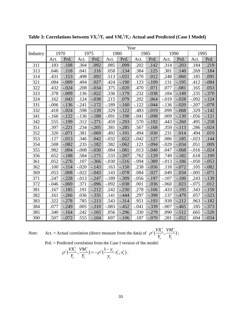
35

Table 3: Correlations between VXci/Yc and VMc

i/Yc: Actual and Predicted (Case I Model)

Industry

Year

1970 1975 1980 1985 1990 1995

Act. Prd. Act. Prd. Act. Prd. Act. Prd. Act. Prd. Act. Prd.

311 .183 .108 .304 .092 .085 .099 .202 .142 .314 .203 .184 .219

313 .646 .118 .041 .116 .058 .134 .384 .125 .381 .140 .269 .184

314 .431 .153 .498 .092 .513 -.021 .670 .012 .248 .060 .185 .095

321 .084 -.009 .494 .027 .424 -.190 .123 -.109 .131 -.195 .412 -.084

322 .432 -.024 .208 -.034 .375 -.020 .470 .071 .077 .081 .165 .053

323 .378 -.009 .136 -.022 .336 -.179 .232 -.038 .184 -.149 .235 -.370

324 .162 .043 .124 -.038 .215 .079 .202 .064 -.019 -.028 -.092 -.124

331 -.006 -.136 -.241 -.172 -.189 -.160 -.122 -.044 -.136 -.020 -.207 -.078

332 .418 -.024 .598 -.139 .329 -.122 .483 -.019 .099 -.068 .329 -.142

341 -.166 -.122 -.136 -.188 -.091 -.190 -.041 -.098 .009 -.130 -.056 -.121

342 .555 -.199 .312 -.271 .459 -.293 .570 -.192 .443 -.260 .495 -.258

351 .397 -.221 .234 -.205 .381 -.285 .567 -.168 .359 -.113 .286 -.024

352 .320 -.071 .381 -.069 .492 -.101 .494 .030 .231 .014 .494 .019

353 .127 -.013 .346 .042 -.032 .022 -.042 .127 .086 .185 -.023 .144

354 .508 -.082 .235 -.182 .382 -.062 .121 -.094 -.029 -.034 .051 .009

355 .982 .004 -.008 -.030 .084 -.081 .013 -.040 .047 -.068 -.016 -.024

356 .652 -.188 .584 -.175 .533 -.207 .762 -.129 .749 -.182 .618 -.199

361 .052 -.276 .107 -.366 -.030 -.516 -.094 -.389 -.013 -.186 -.050 -.053

362 .100 -.114 -.020 -.143 .163 -.150 .238 -.056 .118 -.072 .105 -.082

369 .053 .008 -.022 -.043 .143 -.078 .084 .027 .049 .034 -.005 -.071

371 .247 -.228 -.013 -.247 -.189 -.309 -.056 -.197 -.107 -.100 .243 -.139

372 -.046 -.069 .371 -.096 -.092 -.038 .001 .036 -.060 .023 -.075 .012

381 .167 -.185 .191 -.212 .242 -.230 .278 -.106 .433 -.195 .343 -.159

382 .161 -.266 .036 -.335 .141 -.444 .297 -.398 .137 -.479 .057 -.523

383 .322 -.278 .785 -.213 .543 -.314 .951 -.193 .939 -.212 .963 -.182

384 .077 -.249 .005 -.310 -.083 -.452 -.041 -.339 -.007 -.465 .185 -.373

385 .340 -.164 .242 -.165 .056 -.296 .330 -.279 .090 -.512 .665 -.520

390 .507 -.072 .555 -.104 .697 -.106 .187 -.070 .281 -.052 .694 -.034

Note: Act. = Actual correlation (direct measure from the data) of ( , )i i

i c c

c c

VX VM

Y Y ;

Prd. = Predicted correlation from the Case I version of the model:

1

( , ) ( , )i i

i i i ic c cc c

c c c

VX VM yx x

Y Y y

.

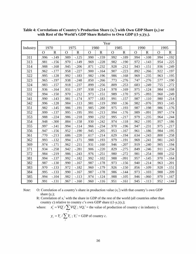
36

Table 4: Correlations of Country’s Production Share (xci) with Own GDP Share (yc) or

with Rest of the World’s GDP Share Relative to Own GDP ((1-yc)/yc).

Industry

Year

1970 1975 1980 1985 1990 1995

O R O R O R O R O R O R

311 .996 -.149 .989 -.125 .990 -.159 .992 -.189 .994 -.108 .994 -.192

313 .981 -.156 .970 -.149 .969 -.228 .982 -.190 .972 -.143 .954 -.225

314 .988 -.168 .945 -.206 .871 -.232 .928 -.212 .943 -.151 .936 -.249

321 .962 -.177 .958 -.227 .900 -.164 .907 -.223 .892 -.266 .922 -.197

322 .995 -.128 .992 -.183 .982 -.196 .986 -.168 .969 -.235 .963 -.195

323 .965 -.197 .938 -.248 .850 -.266 .773 -.276 .747 -.276 .577 -.190

324 .983 -.157 .918 -.237 .899 -.256 .809 -.253 .683 -.249 .755 -.272

331 .936 -.164 .931 -.197 .938 -.214 .978 -.169 .975 -.124 .984 -.168

332 .994 -.150 .970 -.212 .973 -.151 .989 -.170 .975 -.093 .960 -.249

341 .990 -.143 .981 -.174 .977 -.183 .991 -.157 .987 -.110 .980 -.214

342 .996 -.128 .984 -.113 .981 -.119 .990 -.136 .982 -.076 .993 -.145

351 .982 -.145 .986 -.191 .985 -.200 .975 -.193 .987 -.198 .986 -.176

352 .999 -.137 .995 -.195 .991 -.213 .994 -.176 .989 -.091 .997 -.174

353 .988 -.224 .986 -.218 .990 -.232 .995 -.217 .979 -.235 .964 -.244

354 .948 -.300 .884 -.158 .930 -.242 .974 -.118 .962 -.195 .957 -.186

355 .997 -.141 .994 -.114 .966 -.234 .970 -.196 .947 -.231 .975 -.217

356 .947 -.156 .952 -.190 .945 -.205 .953 -.167 .961 -.186 .984 -.195

361 .770 -.213 .686 -.220 .617 -.214 .629 -.194 .634 -.243 .800 -.258

362 .993 -.132 .994 -.171 .988 -.193 .979 -.191 .969 -.241 .981 -.243

369 .974 -.171 .962 -.211 .931 -.160 .946 -.207 .919 -.240 .905 -.194

371 .934 -.258 .942 -.281 .906 -.220 .829 -.275 .849 -.246 .911 -.234

372 .984 -.219 .986 -.243 .976 -.251 .980 -.272 .981 -.254 .988 -.232

381 .994 -.137 .992 -.182 .992 -.102 .988 -.091 .957 -.145 .970 -.164

382 .987 -.130 .990 -.167 .987 -.178 .973 -.156 .940 -.214 .963 -.201

383 .970 -.133 .972 -.182 .960 -.179 .926 -.150 .856 -.109 .928 -.151

384 .995 -.133 .990 -.167 .987 -.178 .986 -.144 .973 -.103 .988 -.209

385 .994 -.104 .982 -.113 .974 -.124 .988 -.105 .946 -.060 .970 -.167

390 .991 -.131 .967 -.160 .960 -.116 .951 -.161 .945 -.113 .952 -.144

Note: O: Correlation of a country’s share in production value (xc

i) with that country’s own GDP

share (yc);

R: Correlation of xci with the share in GDP of the rest of the world (all countries other than

country c) relative to country c’s own GDP share ((1-yc)/yc);

where: /i i i

c c c

c

x VQ VQ ; VQci = the value of production of country c in industry i;

/c c c

c

y Y Y ; Yci = GDP of country c.

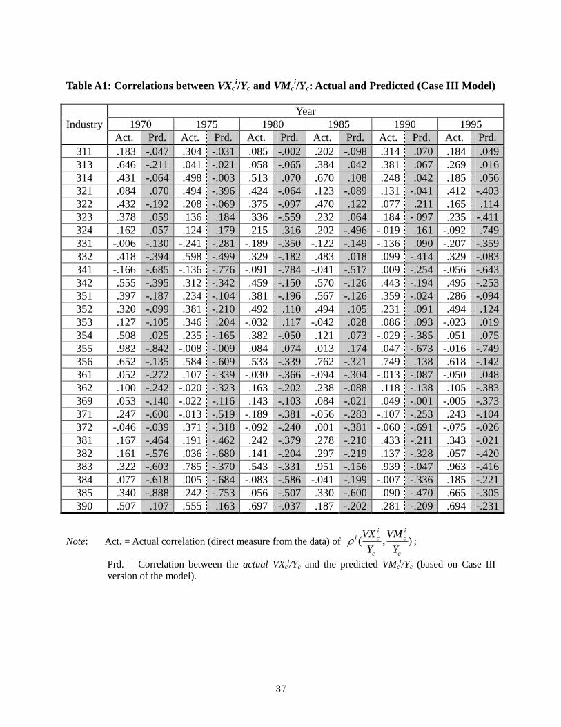
37

Table A1: Correlations between VXci/Yc and VMc

i/Yc: Actual and Predicted (Case III Model)

Industry

Year

1970 1975 1980 1985 1990 1995

Act. Prd. Act. Prd. Act. Prd. Act. Prd. Act. Prd. Act. Prd.

311 .183 -.047 .304 -.031 .085 -.002 .202 -.098 .314 .070 .184 .049

313 .646 -.211 .041 -.021 .058 -.065 .384 .042 .381 .067 .269 .016

314 .431 -.064 .498 -.003 .513 .070 .670 .108 .248 .042 .185 .056

321 .084 .070 .494 -.396 .424 -.064 .123 -.089 .131 -.041 .412 -.403

322 .432 -.192 .208 -.069 .375 -.097 .470 .122 .077 .211 .165 .114

323 .378 .059 .136 .184 .336 -.559 .232 .064 .184 -.097 .235 -.411

324 .162 .057 .124 .179 .215 .316 .202 -.496 -.019 .161 -.092 .749

331 -.006 -.130 -.241 -.281 -.189 -.350 -.122 -.149 -.136 .090 -.207 -.359

332 .418 -.394 .598 -.499 .329 -.182 .483 .018 .099 -.414 .329 -.083

341 -.166 -.685 -.136 -.776 -.091 -.784 -.041 -.517 .009 -.254 -.056 -.643

342 .555 -.395 .312 -.342 .459 -.150 .570 -.126 .443 -.194 .495 -.253

351 .397 -.187 .234 -.104 .381 -.196 .567 -.126 .359 -.024 .286 -.094

352 .320 -.099 .381 -.210 .492 .110 .494 .105 .231 .091 .494 .124

353 .127 -.105 .346 .204 -.032 .117 -.042 .028 .086 .093 -.023 .019

354 .508 .025 .235 -.165 .382 -.050 .121 .073 -.029 -.385 .051 .075

355 .982 -.842 -.008 -.009 .084 .074 .013 .174 .047 -.673 -.016 -.749

356 .652 -.135 .584 -.609 .533 -.339 .762 -.321 .749 .138 .618 -.142

361 .052 -.272 .107 -.339 -.030 -.366 -.094 -.304 -.013 -.087 -.050 .048

362 .100 -.242 -.020 -.323 .163 -.202 .238 -.088 .118 -.138 .105 -.383

369 .053 -.140 -.022 -.116 .143 -.103 .084 -.021 .049 -.001 -.005 -.373

371 .247 -.600 -.013 -.519 -.189 -.381 -.056 -.283 -.107 -.253 .243 -.104

372 -.046 -.039 .371 -.318 -.092 -.240 .001 -.381 -.060 -.691 -.075 -.026

381 .167 -.464 .191 -.462 .242 -.379 .278 -.210 .433 -.211 .343 -.021

382 .161 -.576 .036 -.680 .141 -.204 .297 -.219 .137 -.328 .057 -.420

383 .322 -.603 .785 -.370 .543 -.331 .951 -.156 .939 -.047 .963 -.416

384 .077 -.618 .005 -.684 -.083 -.586 -.041 -.199 -.007 -.336 .185 -.221

385 .340 -.888 .242 -.753 .056 -.507 .330 -.600 .090 -.470 .665 -.305

390 .507 .107 .555 .163 .697 -.037 .187 -.202 .281 -.209 .694 -.231

Note: Act. = Actual correlation (direct measure from the data) of ( , )i i

i c c

c c

VX VM

Y Y ;

Prd. = Correlation between the actual VXci/Yc and the predicted VMc

i/Yc (based on Case III

version of the model).

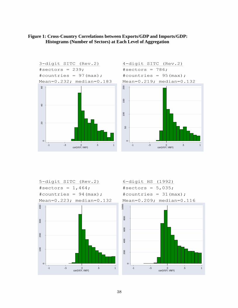
38

Figure 1: Cross-Country Correlations between Exports/GDP and Imports/GDP:

Histograms (Number of Sectors) at Each Level of Aggregation

3-digit SITC (Rev.2)

#sectors = 239;

#countries = 97(max);

Mean=0.232; median=0.183

4-digit SITC (Rev.2)

#sectors = 786;

#countries = 95(max);

Mean=0.219; median=0.132

02

04

06

0

Fre

que

ncy

-1 -.5 0 .5 1corr(VX/Y, VM/Y)

05

01

00

150

200

Fre

que

ncy

-1 -.5 0 .5 1corr(VX/Y, VM/Y)

5-digit SITC (Rev.2)

#sectors = 1,464;

#countries = 94(max);

Mean=0.223; median=0.132

6-digit HS (1992)

#sectors = 5,035;

#countries = 31(max);

Mean=0.209; median=0.116

0

100

200

300

400

Fre

que

ncy

-1 -.5 0 .5 1corr(VX/Y, VM/Y)

0

200

400

600

800

100

0

Fre

que

ncy

-1 -.5 0 .5 1corr(VX/Y, VM/Y)

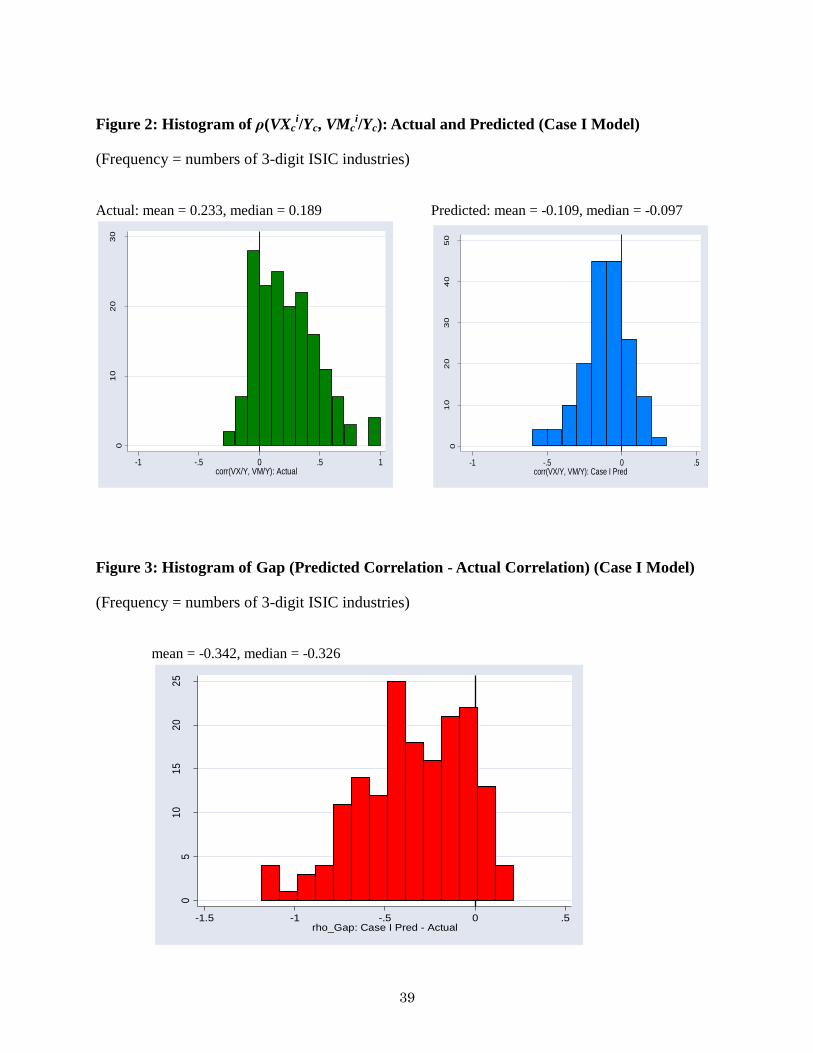
39

Figure 2: Histogram of ρ(VXci/Yc, VMc

i/Yc): Actual and Predicted (Case I Model)

(Frequency = numbers of 3-digit ISIC industries)

Actual: mean = 0.233, median = 0.189 Predicted: mean = -0.109, median = -0.097

01

02

03

0

Fre

que

ncy

-1 -.5 0 .5 1corr(VX/Y, VM/Y): Actual

01

02

03

04

05

0

Fre

que

ncy

-1 -.5 0 .5corr(VX/Y, VM/Y): Case I Pred

Figure 3: Histogram of Gap (Predicted Correlation - Actual Correlation) (Case I Model)

(Frequency = numbers of 3-digit ISIC industries)

mean = -0.342, median = -0.326

05

10

15

20

25

Fre

que

ncy

-1.5 -1 -.5 0 .5rho_Gap: Case I Pred - Actual

40

Figure A1: Histogram of ρ(VXci/Yc, VMc

i/Yc): Actual and Predicted (Case III Model)

(Frequency = numbers of 3-digit ISIC industries)

Actual: mean = 0.233, median = 0.189 Predicted: mean = -0.194, median = -0.153

01

02

03

0

Fre

que

ncy

-1 -.5 0 .5 1corr(VX/Y, VM/Y): Actual

01

02

03

0

Fre

que

ncy

-1 -.5 0 .5 1corr(VX/Y, VM/Y): Case III Pred

Figure A2: Histogram of Gap (Predicted Correlation - Actual Correlation) (Case III Model)

(Frequency = numbers of 3-digit ISIC industries)

mean = -0.745, median = -1.080

05

10

15

20

Fre

que

ncy

-2 -1 0 1rho_Gap: Case III Pred - Actual

i

Appendix C-1

This appendix shows how the sets of equations in Section 3 are derived for each of the three

cases (Case I, II and III). Derivation of the common equations (Equations (1) through (9)) to all

the cases is as explained in Section 3.

Case I

Derivation of Equations (8-I) through (12-I) is shown in Section 3.

For Equation (13-I), from Equation (11-I);

)(1

'

'

cc

c

c

cc

c YN

nb

YY

VX.

Define yc ≡ Yc/Yw. Also note that cw

cc

c YYY '

' . Hence;

N

nb

y

yYy

N

nb

YyY

VX c

c

c

wc

c

wcc

c )1()1(

1 .

Define xc ≡ VQc/VQw. In this Case I, since all firms (in an industry) in the world charge the same

price and produce the same amount, VQc = ncpq and VQw = Npq, so that xc = nc/N. Therefore;

c

c

c

c

c bxy

y

Y

VX )1( .

Finally, by market clearing in an industry, the value of the total world production must equal the

world total expenditure. That is;

wwww YVQbbYVQ / .

Hence;

c

c

c

w

w

c

c xy

y

Y

VQ

Y

VX )1( . (13-I)

For Equation (14-I), from Equation (12-I);

)1()(1

N

nb

N

nNbY

YY

VM cc

c

cc

c

.

Hence, since xc = nc/N and b = VQw/Yw as shown above;

)1( c

w

w

c

c xY

VQ

Y

VX . (14-I)

Case II

Equations (8-II) through (14-II) for Case II are derived as follows:

In this case, since the prices of all the varieties charged by firms (excluding trade cost)

are the same, p(ω) = p for all ω. Thus, from Equation (8);

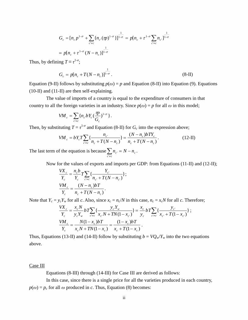
ii

1

1

1

1

1

'

'

11

1

'

1

'

1

)]([

][]})({[

cc

cc

cc

cc

ccc

nNnp

nnppnpnG

Thus, by defining T ≡ τ1-σ

;

1

1

)]([ ccc nNTnpG . (8-II)

Equation (9-II) follows by substituting p(ω) = p and Equation (8-II) into Equation (9). Equations

(10-II) and (11-II) are then self-explaining.

The value of imports of a country is equal to the expenditure of consumers in that

country to all the foreign varieties in an industry. Since p(ω) = p for all ω in this model;

cc c

cccG

pbYnVM

'

1

' })({ .

Then, by substituting T = τ1-σ

and Equation (8-II) for Gc into the expression above;

)(

)(}

)({

'

'

cc

cc

cc cc

c

ccnNTn

bTYnN

nNTn

nTbYVM

. (12-II)

The last term of the equation is because c

cc

c nNn '

' .

Now for the values of exports and imports per GDP: from Equations (11-II) and (12-II);

cc cc

c

c

c

c

c

nNTn

YT

Y

bn

Y

VX

' ''

' })(

{ ;

)(

)(

cc

c

c

c

nNTn

bTnN

Y

VM

.

Note that Yc = ycYw for all c. Also, since xc = nc/N in this case, nc = xcN for all c. Therefore;

cc cc

c

c

c

cc cc

wc

wc

c

c

c

xTx

ybT

y

x

xTNNx

YybT

Yy

Nx

Y

VX

' ''

'

' ''

' })1(

{})1(

{ ;

)1(

)1(

)1(

)1(

cc

c

cc

c

c

c

xTx

bTx

xTNNx

bTxN

Y

VM

.

Thus, Equations (13-II) and (14-II) follow by substituting b = VQw/Yw into the two equations

above.

Case III

Equations (8-III) through (14-III) for Case III are derived as follows:

In this case, since there is a single price for all the varieties produced in each country,

p(ω) = pc for all ω produced in c. Thus, Equation (8) becomes:

iii

1

1

'

1

''

1 ]})({[cc

ccccc pnpnG .

Then, Equation (8-III) follows by defining T ≡ τ1-σ

. Thus, each firm in country c earns the same

revenue (or produces the same value of output), which is, by substituting Equation (8-III) into

Equation (9):

]}})({

{[})({

})({)(

'

'"

1

""

1

''

11

'

'

1

''

1

1

'

1

'

'

1

cc

cc

cccc

c

c

cc

cccc

c

c

cc c

c

c

c

c

ccc

pnTpn

pYb

pnTpn

pbY

G

pbY

G

pbYqp

.

Equation (9-III) then follows by substituting T = τ1-σ

into the expression above. Equation (10-III)

also follows by substituting (9-III) into the expression of the value of the total output in country

c: VQc = ncpcqc. The expression for the value of total exports from country c, Equation (11-III), is

obvious since the second term of RHS of Equation (10-III) is the value exported abroad, while

the first term is the value consumed domestically. On the other hand, since the value of imports

is equal to the expenditure of consumers in country c to all the foreign varieties in an industry;

1

'

1

''

1

'

1'

'

})({

})({c

cc

ccc

cc c

c

cccG

pnbY

G

pbYnVM .

Then, Equation (12-III) is obtained by substituting T = τ1-σ

and Equation (8-III) for Gc into the

expression above.

Now the expressions for the values of exports and imports per GDP are derived as

follows. From Equations (11-III) and (12-III);

cc cc

cc

cccc

c

c

cc

cc

cccc

wc

wc

cc

cc

cc

cccc

c

c

cc

c

c

pnTpn

ybT

y

pn

pnTpn

YybT

Yy

pn

pnTpn

YbT

Y

pn

Y

VX

' '

'"

1

""

1

''

'

1

'"

1

""

1

''

'

1

'

'"

1

""

1

''

'

1

})(

{})(

{

})(

{

cc

cccc

cc

cc

c

c

pnTpn

pnbT

Y

VM

'

1

''

1

'

1

''

)(

)(

.

The second equality in the former expression (VXc/Yc) is because Yc = ycYw for all c. Then,

Equations (13-III) and (14-III) are derived by substituting b = VQw/Yw into the two expressions

above.

Finally, consider the two-country version of the model for this Case III. In the

two-country setting, there is only one foreign country for country c (home), which is ‘the rest of

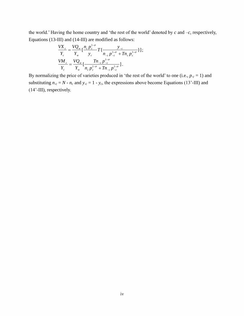
iv

the world.’ Having the home country and ‘the rest of the world’ denoted by c and –c, respectively,

Equations (13-III) and (14-III) are modified as follows:

}]{[11

1

cccc

c

c

cc

w

w

c

c

pTnpn

yT

y

pn

Y

VQ

Y

VX;

][11

1

cccc

cc

w

w

c

c

pTnpn

pTn

Y

VQ

Y

VM.

By normalizing the price of varieties produced in ‘the rest of the world’ to one (i.e., p-c = 1) and

substituting n-c = N - nc and y-c = 1 - yc, the expressions above become Equations (13’-III) and

(14’-III), respectively.

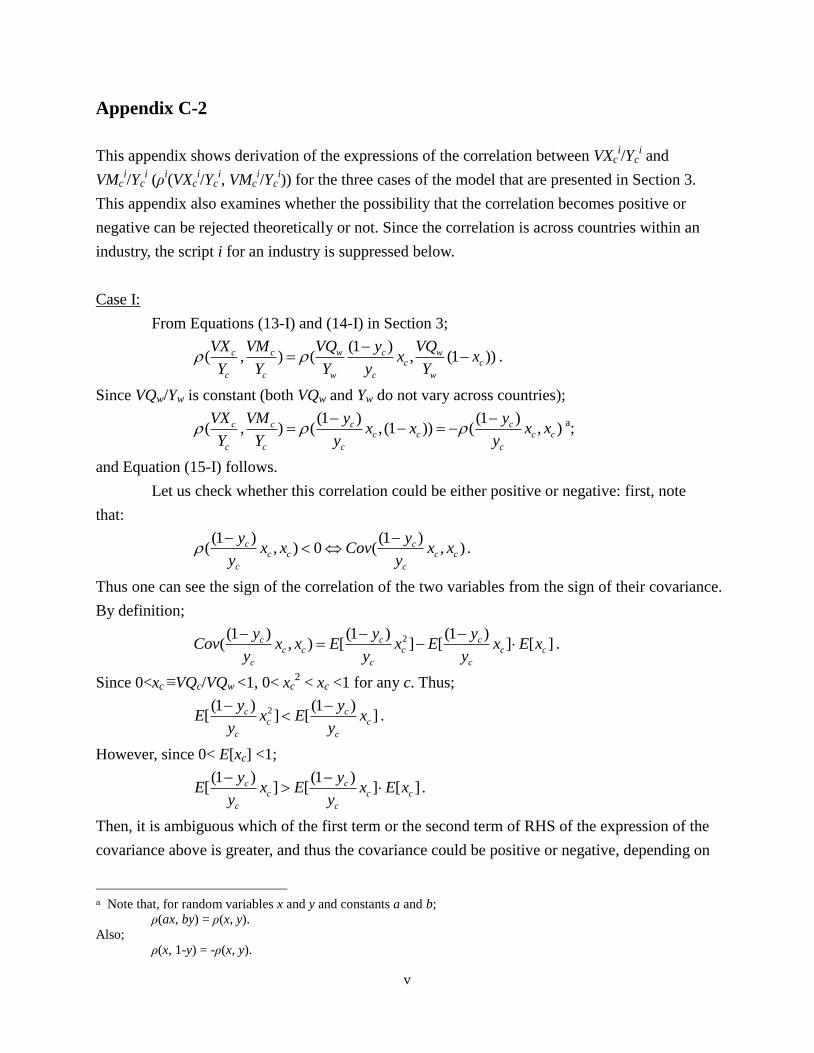
v

Appendix C-2

This appendix shows derivation of the expressions of the correlation between VXci/Yc

i and

VMci/Yc

i (ρ

i(VXc

i/Yc

i, VMc

i/Yc

i)) for the three cases of the model that are presented in Section 3.

This appendix also examines whether the possibility that the correlation becomes positive or

negative can be rejected theoretically or not. Since the correlation is across countries within an

industry, the script i for an industry is suppressed below.

Case I:

From Equations (13-I) and (14-I) in Section 3;

(1 )( , ) ( , (1 ))c c w c w

c c

c c w c w

VX VM VQ y VQx x

Y Y Y y Y

.

Since VQw/Yw is constant (both VQw and Yw do not vary across countries);

(1 ) (1 )( , ) ( , (1 )) ( , )c c c c

c c c c

c c c c

VX VM y yx x x x

Y Y y y

a;

and Equation (15-I) follows.

Let us check whether this correlation could be either positive or negative: first, note

that:

(1 ) (1 )( , ) 0 ( , )c c

c c c c

c c

y yx x Cov x x

y y

.

Thus one can see the sign of the correlation of the two variables from the sign of their covariance.

By definition;

2(1 ) (1 ) (1 )( , ) [ ] [ ] [ ]c c c

c c c c c

c c c

y y yCov x x E x E x E x

y y y

.

Since 0<xc ≡VQc/VQw <1, 0< xc2 < xc <1 for any c. Thus;

2(1 ) (1 )[ ] [ ]c c

c c

c c

y yE x E x

y y

.

However, since 0< E[xc] <1;

(1 ) (1 )[ ] [ ] [ ]c c

c c c

c c

y yE x E x E x

y y

.

Then, it is ambiguous which of the first term or the second term of RHS of the expression of the

covariance above is greater, and thus the covariance could be positive or negative, depending on

a Note that, for random variables x and y and constants a and b;

ρ(ax, by) = ρ(x, y).

Also;

ρ(x, 1-y) = -ρ(x, y).

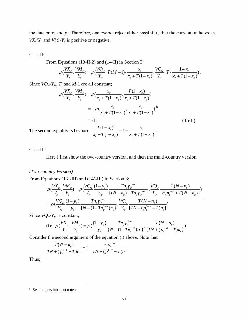
vi

the data on xc and yc. Therefore, one cannot reject either possibility that the correlation between

VXc/Yc and VMc/Yc is positive or negative.

Case II:

From Equations (13-II-2) and (14-II) in Section 3;

1( , ) ( ( 1) , )

(1 ) (1 )

c c w c w c

c c w c c w c c

VX VM VQ x VQ xT M T

Y Y Y x T x Y x T x

.

Since VQw/Yw, T, and M-1 are all constant;

(1 )( , ) ( , )

(1 ) (1 )

c c c c

c c c c c c

VX VM x T x

Y Y x T x x T x

( , )(1 ) (1 )

c c

c c c c

x x

x T x x T x

b

= -1. (15-II)

The second equality is because (1 )

1(1 ) (1 )

c c

c c c c

T x x

x T x x T x

.

Case III:

Here I first show the two-country version, and then the multi-country version.

(Two-country Version)

From Equations (13’-III) and (14’-III) in Section 3;

1

1 1

1

1 1

(1 ) ( )( , ) ( , )

{( ) } { ( )}

(1 ) ( )( , )

{ (1 ) } { ( ) }

c c w c c c w c

c c w c c c c w c c c

w c c c w c

w c c c w c c

VX VM VQ y Tn p VQ T N n

Y Y Y y N n Tn p Y n p T N n

VQ y Tn p VQ T N n

Y y N Tp n Y TN p T n

.

Since VQw/Yw is constant;

(i): 1

1 1

(1 ) ( )( , ) ( , )

{ (1 ) } { ( ) }

c c c c c c

c c c c c c c

VX VM y Tn p T N n

Y Y y N Tp n TN p T n

.

Consider the second argument of the equation (i) above. Note that:

1

1 1

( )1

( ) ( )

c c c

c c c c

T N n n p

TN p T n TN p T n

.

Thus;

b See the previous footnote a.

vii

(ii):

1

1 1

1 1

1 1

(1 ) ( )( , )

{ (1 ) } { ( ) }

(1 )( , )

{ (1 ) } ( )

c c c c

c c c c c

c c c c c

c c c c c

y Tn p T N n

y N Tp n TN p T n

y Tn p n p

y N Tp n TN p T n

On the other hand;

(iii):

1

1 1

1

1 1

(1 ) ( )( , )

{ (1 ) } { ( ) }

(1 )( , )

{ (1 ) } ( )

c c c c

c c c c c

c c c c

c c c c c

y Tn p T N n

y N Tp n TN p T n

y n p N n

y N Tp n TN p T n

since T ≡ τ1-σ

is constant.

Therefore, by combining (i), (ii), and (iii) above, Equation (15’-III) is derived as follows: 1

1 1

1 1

1 1

(1 )( , ) ( , )

{ (1 ) } ( )

(1 )( , )

{ (1 ) } ( )

c c c c c c

c c c c c c c

c c c c c

c c c c c

VX VM y n p N n

Y Y y N Tp n TN p T n

y Tn p n p

y N Tp n TN p T n

(15’-III)

Now check whether this correlation could be either positive or negative. Since:

1 1

1 1

(1 )( , ) 0

{ (1 ) } ( )

c c c c c

c c c c c

y Tn p n p

y N Tp n TN p T n

0))(

,})1({

)1((

1

1

1

1

cc

cc

cc

cc

c

c

nTpTN

pn

nTpN

pTn

y

yCov

;

the sign of the correlation of the two variables is the same as that of their covariance. By

definition;

1 1

1 1

1 1

1 1

1 1

1 1

(1 )( , )

{ (1 ) } ( )

(1 )[ ]

{ (1 ) }{ ( ) }

(1 )[ ] [ ]

{ (1 ) } ( )

c c c c c

c c c c c

c c c c c

c c c c c

c c c c c

c c c c c

y Tn p n pCov

y N Tp n TN p T n

y Tn p n pE

y N Tp n TN p T n

y Tn p n pE E

y N Tp n TN p T n

Note that:

1 1

1 11

( ) ( )

c c c c

c c c c c

n p n p

TN p T n n p N n T

for any nc, pc

since the term (N – nc)T in the denominator above is positive. Hence;

1 1 1

1 1 1

(1 ) (1 )

{ (1 ) } { ( ) } { (1 ) }

c c c c c c c c

c c c c c c c c

y Tn p n p y Tn pc

y N Tp n TN p T n y N Tp n

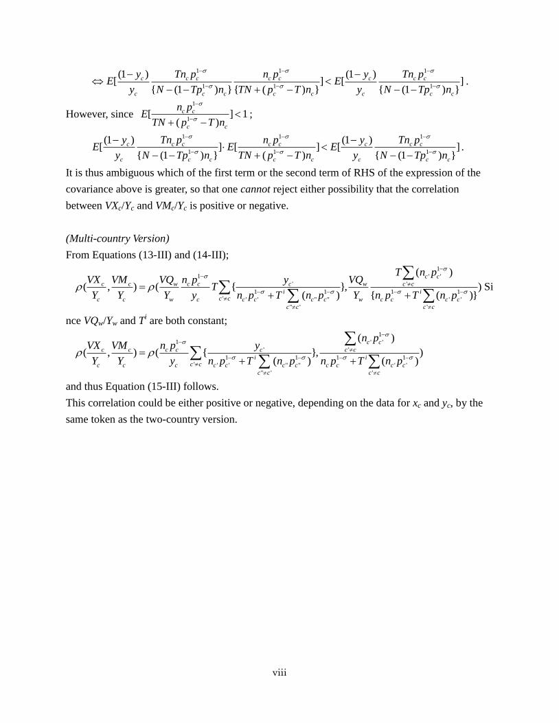
viii

1 1 1

1 1 1

(1 ) (1 )[ ] [ ]

{ (1 ) } { ( ) } { (1 ) }

c c c c c c c c

c c c c c c c c

y Tn p n p y Tn pE E

y N Tp n TN p T n y N Tp n

.

However, since 1

1[ ] 1

( )

c c

c c

n pE

TN p T n

;

1 1 1

1 1 1

(1 ) (1 )[ ] [ ] [ ]

{ (1 ) } ( ) { (1 ) }

c c c c c c c c

c c c c c c c c

y Tn p n p y Tn pE E E

y N Tp n TN p T n y N Tp n

.

It is thus ambiguous which of the first term or the second term of RHS of the expression of the

covariance above is greater, so that one cannot reject either possibility that the correlation

between VXc/Yc and VMc/Yc is positive or negative.

(Multi-country Version)

From Equations (13-III) and (14-III); 1

1 ' '

' '

1 1 1 1' ' ' " " ' '

" ' '

( )

( , ) ( { }, )( ) { ( )}

c c

c c w c c c w c c

i ic cc c w c c c c c w c c c c

c c c c

T n pVX VM VQ n p y VQ

TY Y Y y n p T n p Y n p T n p

Si

nce VQw/Yw and Ti are both constant;

1

1 ' '

' '

1 1 1 1' ' ' " " ' '

" ' '

( )

( , ) ( { }, )( ) ( )

c c

c c c c c c c

i ic cc c c c c c c c c c c

c c c c

n pVX VM n p y

Y Y y n p T n p n p T n p

and thus Equation (15-III) follows.

This correlation could be either positive or negative, depending on the data for xc and yc, by the

same token as the two-country version.

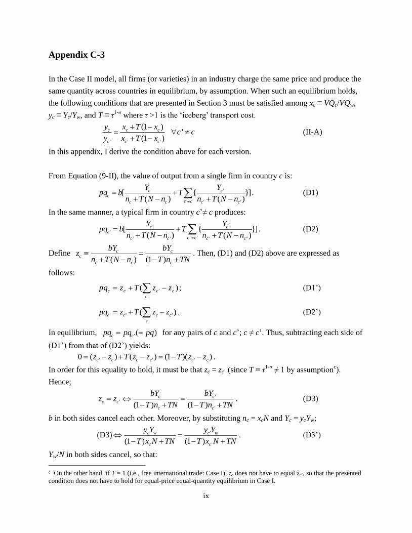
ix

Appendix C-3

In the Case II model, all firms (or varieties) in an industry charge the same price and produce the

same quantity across countries in equilibrium, by assumption. When such an equilibrium holds,

the following conditions that are presented in Section 3 must be satisfied among xc ≡ VQc/VQw,

yc ≡ Yc/Yw, and T ≡ τ1-σ

where τ >1 is the ‘iceberg’ transport cost.

' ' '

(1 )

(1 )

c c c

c c c

y x T x

y x T x

'c c (II-A)

In this appendix, I derive the condition above for each version.

From Equation (9-II), the value of output from a single firm in country c is:

'

' ' '

[ { }]( ) ( )

c cc

c cc c c c

Y Ypq b T

n T N n n T N n

. (D1)

In the same manner, a typical firm in country c’≠ c produces:

' "'

" '' ' " "

[ { }]( ) ( )

c cc

c cc c c c

Y Ypq b T

n T N n n T N n

. (D2)

Define ( ) (1 )

c cc

c c c

bY bYz

n T N n T n TN

. Then, (D1) and (D2) above are expressed as

follows:

)('

' c

c

ccc zzTzpq ; (D1’)

' ' '( )c c c c

c

pq z T z z . (D2’)

In equilibrium, '( )c cpq pq pq for any pairs of c and c’; c ≠ c’. Thus, subtracting each side of

(D1’) from that of (D2’) yields:

' ' '0 ( ) ( ) (1 )( )c c c c c cz z T z z T z z .

In order for this equality to hold, it must be that zc = zc’ (since T ≡ τ1-σ

≠ 1 by assumptionc).

Hence;

''

'(1 ) (1 )

c cc c

c c

bY bYz z

T n TN T n TN

. (D3)

b in both sides cancel each other. Moreover, by substituting nc = xcN and Yc = ycYw;

(D3) '

'(1 ) (1 )

c w c w

c c

y Y y Y

T x N TN T x N TN

. (D3’)

Yw/N in both sides cancel, so that:

c On the other hand, if T = 1 (i.e., free international trade: Case I), zc does not have to equal zc’, so that the presented

condition does not have to hold for equal-price equal-quantity equilibrium in Case I.

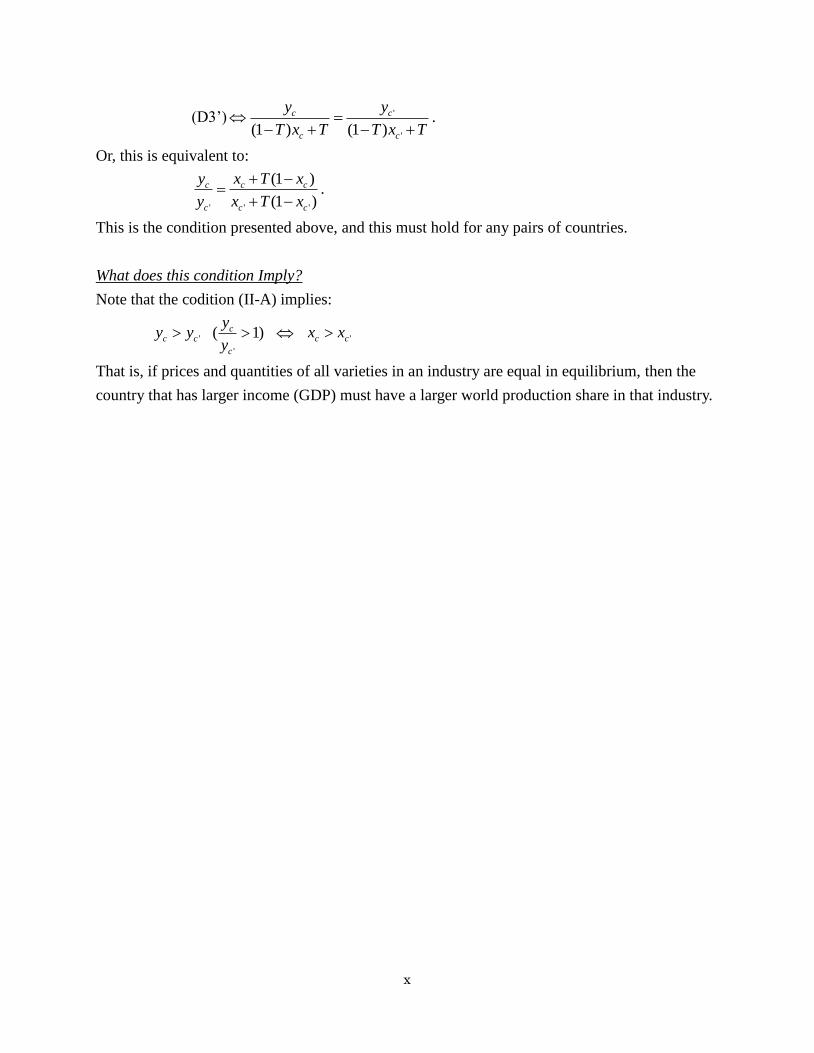
x

(D3’) '

'(1 ) (1 )

c c

c c

y y

T x T T x T

.

Or, this is equivalent to:

' ' '

(1 )

(1 )

c c c

c c c

y x T x

y x T x

.

This is the condition presented above, and this must hold for any pairs of countries.

What does this condition Imply?

Note that the codition (II-A) implies:

'c cy y '

( 1)c

c

y

y 'c cx x

That is, if prices and quantities of all varieties in an industry are equal in equilibrium, then the

country that has larger income (GDP) must have a larger world production share in that industry.

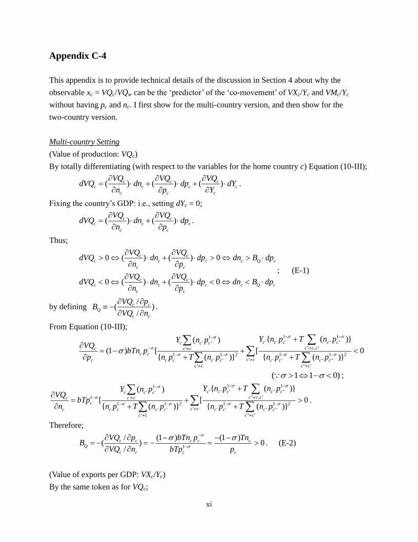
xi

Appendix C-4

This appendix is to provide technical details of the discussion in Section 4 about why the

observable xc = VQc/VQw can be the ‘predictor’ of the ‘co-movement’ of VXc/Yc and VMc/Yc

without having pc and nc. I first show for the multi-country version, and then show for the

two-country version.

Multi-country Setting

(Value of production: VQc)

By totally differentiating (with respect to the variables for the home country c) Equation (10-III);

( ) ( ) ( )c c cc c c c

c c c

VQ VQ VQdVQ dn dp dY

n p Y

.

Fixing the country’s GDP: i.e., setting dYc = 0;

( ) ( )c cc c c

c c

VQ VQdVQ dn dp

n p

.

Thus;

0 ( ) ( ) 0

0 ( ) ( ) 0

c cc c c c Q c

c c

c cc c c c Q c

c c

VQ VQdVQ dn dp dn B dp

n p

VQ VQdVQ dn dp dn B dp

n p

; (E-1)

by defining /

( )/

c cQ

c c

VQ pB

VQ n

.

From Equation (10-III);

1 11' ' ' " "' '

" , ''

1 1 2 1 1 2'' ' ' ' " "

' " '

{ ( )}( )

(1 ) [ [ 0{ ( )} { ( )}

c c c c cc c cc c cc c c

c c

c cc c c c c c c c c

c c c c

Y n p T n pY n pVQ

bTn pp n p T n p n p T n p

( 1 1 0) ;

1 11' ' ' " "' '

" , '1 '

1 1 2 1 1 2'' ' ' ' " "

' " '

{ ( )}( )

[ [ 0{ ( )} { ( )}

c c c c cc c cc c cc c c

c

c cc c c c c c c c c

c c c c

Y n p T n pY n pVQ

bTpn n p T n p n p T n p

.

Therefore;

1

/ (1 ) (1 )( ) 0

/

c c c c cQ

c c c c

VQ p bTn p TnB

VQ n bTp p

. (E-2)

(Value of exports per GDP: VXc/Yc)

By the same token as for VQc;

xii

( / ) ( / )( ) 0 ( ) ( ) 0

( / ) ( / )( ) 0 ( ) ( ) 0

c c c c cc c c X c

c c c

c c c c cc c c X c

c c c

VX VX Y VX Yd dn dp dn B dp

Y n p

VX VX Y VX Yd dn dp dn B dp

Y n p

(E-3)

by defining ( / ) /

( )( / ) /

c c cX

c c c

VX Y pB

VX Y n

.

Note that:

(17-III):

1 1

' ' ' " "

" , '

1 1 2' ' ' " "

" '

{ ( )}( / ) (1 )

[ 0{ ( )}

c c c c c

c c cc c W c c

c cc W c c c c c

c c

y n p T n pVX Y VQ Tn p

p Y y n p T n p

;

(15-III):

1 1

' ' ' " "1" , '

1 1 2' ' ' " "

" '

{ ( )}( / )

[ 0{ ( )}

c c c c c

c c cc c W c

c cc W c c c c c

c c

y n p T n pVX Y VQ Tp

n Y y n p T n p

.

Therefore;

1

( / )(1 )

(1 )0

( / )

c c wc c

c w c cX

c c w cc

c w c

VX Y VQTn p

p Y y TnB

VX Y VQ pTp

n Y y

. (E-4)

(Value of imports per GDP: VMc/Yc)

By the same token;

( / ) ( / )( ) 0 ( ) ( ) 0

( / ) ( / )( ) 0 ( ) ( ) 0

c c c c cc c c M c

c c c

c c c c cc c c M c

c c c

VM VM Y VM Yd dn dp dn B dp

Y n p

VM VM Y VM Yd dn dp dn B dp

Y n p

(E-5)

by defining ( / ) /

( )( / ) /

c c cM

c c c

VM Y pB

VM Y n

. Notice the sign of the last inequality in each of the two

lines above: this is because ( / ) / 0c c cVM Y n as shown below.

Note that:

(19-III):

1

' '

'

1 1 2

' '

'

(1 ) { ( )}( / )

0{ ( )}

c c c c

c c w c c

c w c c c c

c c

T n p n pVM Y VQ

p Y n p T n p

;

(17-III):

1 1

' '

'

1 1 2

' '

'

( )( / )

0{ ( )}

c c c

c c w c c

c w c c c c

c c

Tp n pVM Y VQ

n Y n p T n p

.

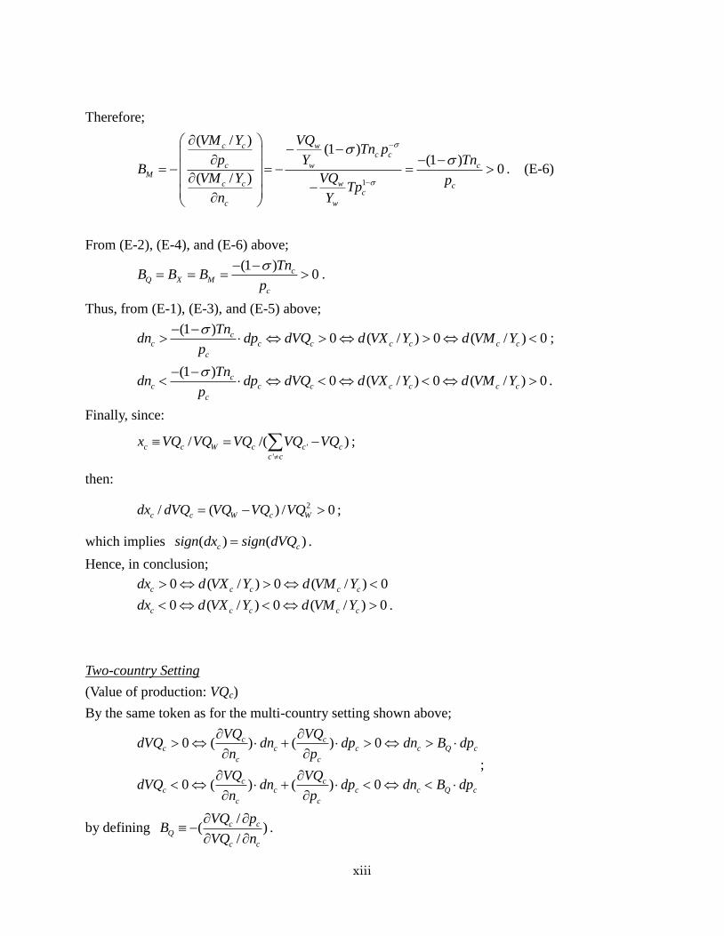
xiii

Therefore;

1

( / )(1 )

(1 )0

( / )

c c wc c

c w cM

c c w cc

c w

VM Y VQTn p

p Y TnB

VM Y VQ pTp

n Y

. (E-6)

From (E-2), (E-4), and (E-6) above;

(1 )

0cQ X M

c

TnB B B

p

.

Thus, from (E-1), (E-3), and (E-5) above;

(1 )

0 ( / ) 0 ( / ) 0cc c c c c c c

c

Tndn dp dVQ d VX Y d VM Y

p

;

(1 )

0 ( / ) 0 ( / ) 0cc c c c c c c

c

Tndn dp dVQ d VX Y d VM Y

p

.

Finally, since:

'

'

/ /( )c c W c c c

c c

x VQ VQ VQ VQ VQ

;

then:

2/ ( ) / 0c c W c Wdx dVQ VQ VQ VQ ;

which implies ( ) ( )c csign dx sign dVQ .

Hence, in conclusion;

0 ( / ) 0 ( / ) 0c c c c cdx d VX Y d VM Y

0 ( / ) 0 ( / ) 0c c c c cdx d VX Y d VM Y .

Two-country Setting

(Value of production: VQc)

By the same token as for the multi-country setting shown above;

0 ( ) ( ) 0

0 ( ) ( ) 0

c cc c c c Q c

c c

c cc c c c Q c

c c

VQ VQdVQ dn dp dn B dp

n p

VQ VQdVQ dn dp dn B dp

n p

;

by defining /

( )/

c cQ

c c

VQ pB

VQ n

.

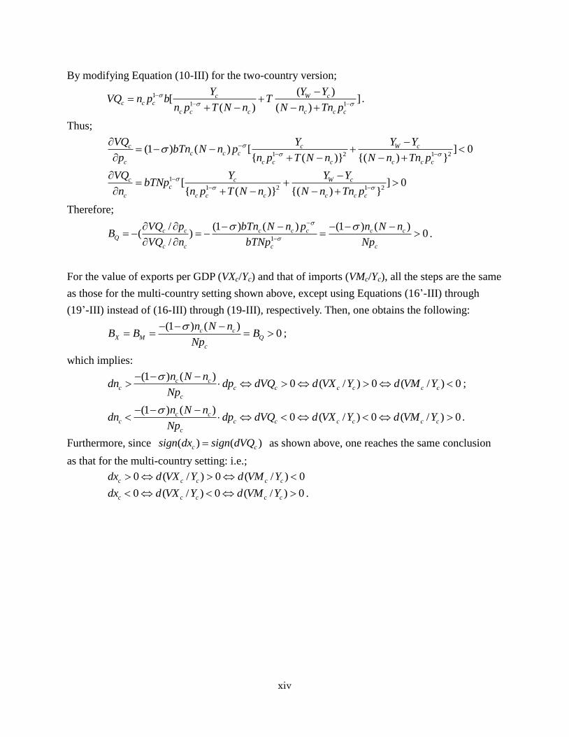
xiv

By modifying Equation (10-III) for the two-country version;

1

1 1

( )[ ]

( ) ( )

c W cc c c

c c c c c c

Y Y YVQ n p b T

n p T N n N n Tn p

.

Thus;

1 2 1 2(1 ) ( ) [ ] 0

{ ( )} {( ) }

c c W cc c c

c c c c c c c

VQ Y Y YbTn N n p

p n p T N n N n Tn p

1

1 2 1 2[ ] 0{ ( )} {( ) }

c c W cc

c c c c c c c

VQ Y Y YbTNp

n n p T N n N n Tn p

Therefore;

1

/ (1 ) ( ) (1 ) ( )( ) 0

/

c c c c c c cQ

c c c c

VQ p bTn N n p n N nB

VQ n bTNp Np

.

For the value of exports per GDP (VXc/Yc) and that of imports (VMc/Yc), all the steps are the same

as those for the multi-country setting shown above, except using Equations (16’-III) through

(19’-III) instead of (16-III) through (19-III), respectively. Then, one obtains the following:

(1 ) ( )

0c cX M Q

c

n N nB B B

Np

;

which implies:

(1 ) ( )

0 ( / ) 0 ( / ) 0c cc c c c c c c

c

n N ndn dp dVQ d VX Y d VM Y

Np

;

(1 ) ( )

0 ( / ) 0 ( / ) 0c cc c c c c c c

c

n N ndn dp dVQ d VX Y d VM Y

Np

.

Furthermore, since ( ) ( )c csign dx sign dVQ as shown above, one reaches the same conclusion

as that for the multi-country setting: i.e.;

0 ( / ) 0 ( / ) 0c c c c cdx d VX Y d VM Y

0 ( / ) 0 ( / ) 0c c c c cdx d VX Y d VM Y .