A Concrete Final Coalgebra Theoremfor ZF Set Theory?

Lawrence C. Paulsonlcp@cl.cam.ac.uk

Computer Laboratory, University of Cambridge, England

Abstract. A special final coalgebra theorem, in the style of Aczel’s [2],is proved within standard Zermelo-Fraenkel set theory. Aczel’s Anti-Foundation Axiom is replaced by a variant definition of function thatadmits non-well-founded constructions. Variant ordered pairs and tuples,of possibly infinite length, are special cases of variant functions. Ana-logues of Aczel’s Solution and Substitution Lemmas are proved in thestyle of Rutten and Turi [12]. The approach is less general than Aczel’s,but the treatment of non-well-founded objects is simple and concrete.The final coalgebra of a functor is its greatest fixedpoint. The theory isintended for machine implementation and a simple case of it is alreadyimplemented using the theorem prover Isabelle [10].

? Thomas Forster alerted me to Quine’s work. Peter Aczel and Andrew Pitts offeredconsiderable advice and help. Daniele Turi gave advice by electronic mail. I haveused Paul Taylor’s macros for commuting diagrams. K. Mukai commented on thetext. Research funded by the ESPRIT Basic Research Action 6453 ‘Types.’

Table of Contents

1 Introduction . . . . . . . . . . . . . . . . . . . . . . . . . . . . . . . 1

2 An Alternative Definition of Pairs and Functions . . . . . . . . 22.1 Quine’s Ordered Pairs . . . . . . . . . . . . . . . . . . . . . . . . 22.2 Basic Definitions and Properties . . . . . . . . . . . . . . . . . . 42.3 Basic Properties of the Cumulative Hierarchy . . . . . . . . . . . 5

3 A Final Coalgebra . . . . . . . . . . . . . . . . . . . . . . . . . . . 73.1 The Functor Q and the Set U . . . . . . . . . . . . . . . . . . . . 73.2 U is a Final Coalgebra . . . . . . . . . . . . . . . . . . . . . . . . 9

4 Solutions of Equations . . . . . . . . . . . . . . . . . . . . . . . . . 104.1 Preliminaries: the Binary Sum Functor . . . . . . . . . . . . . . 104.2 An Expanded Version of U . . . . . . . . . . . . . . . . . . . . . 114.3 An Embedding . . . . . . . . . . . . . . . . . . . . . . . . . . . . 124.4 Substitution . . . . . . . . . . . . . . . . . . . . . . . . . . . . . 134.5 Solution and Substitution Lemmas . . . . . . . . . . . . . . . . . 134.6 Special Final Coalgebra Theorem . . . . . . . . . . . . . . . . . . 15

5 Functors Uniform on Maps . . . . . . . . . . . . . . . . . . . . . . 165.1 The Constant Functor . . . . . . . . . . . . . . . . . . . . . . . . 165.2 Binary Product . . . . . . . . . . . . . . . . . . . . . . . . . . . . 165.3 Binary Sum . . . . . . . . . . . . . . . . . . . . . . . . . . . . . . 175.4 Sum of a Family of Sets . . . . . . . . . . . . . . . . . . . . . . . 185.5 Product of a Family of Sets . . . . . . . . . . . . . . . . . . . . . 195.6 The Identity Functor . . . . . . . . . . . . . . . . . . . . . . . . 20

6 Conclusions . . . . . . . . . . . . . . . . . . . . . . . . . . . . . . . . 20

A Proof of Prop. 21 . . . . . . . . . . . . . . . . . . . . . . . . . . . . 23

1 Introduction

A recurring issue in theoretical computer science is the treatment of infinitecomputations. One important approach is based upon the final coalgebra. Thiscategory-theoretic notion relates to the methods of bisimulation and coinduction,which are heavily used in concurrency theory [6], functional programming [1] andoperational semantics [7].

Aczel and Mendler [3] and also Barr [4] have proved that final coalgebrasexist in set theory for large classes of naturally occurring functors. This mightbe supposed to satisfy most people’s requirements. But Aczel [2] has argued thecase for a non-standard set theory in which infinite computations, and othernon-well-founded phenomena, can be modelled directly. He proposes to replaceset theory’s Foundation Axiom (FA) by an Anti-Foundation Axiom (AFA) thatguarantees the existence of solutions to x = {x} and more generally of all systemsof equations of the form xi = {xi, xj , . . .}. His general final coalgebra theoremserves as a model construction to justify AFA.

Under AFA, a suitable functor F does not merely have a final coalgebra. Thatfinal coalgebra equals F ’s greatest fixedpoint. This is the natural dual of thetheorem that a functor’s initial algebra is its least fixedpoint. These fixedpointsare exact, not up to isomorphism.

The elements of the final coalgebra are easily visualised. For instance, thefunctor A×− (the functor F such that F (Z) = A×Z on objects) yields the setof streams over A. The final coalgebra is also the greatest solution of S = A×S.If s ∈ S then

s = 〈a1, s1〉, s1 = 〈a2, s2〉, s2 = 〈a3, s3〉, . . . ;

s is the infinite stream 〈a1, 〈a2, 〈a3, . . .〉〉〉.In standard set theory, the Foundation Axiom (FA) outlaws infinite descents

under the membership relation. Under the standard definition of ordered pairwe have b ∈ {a, b} ∈ 〈a, b〉. Infinitely nested pairs such as s above would cre-ate infinite ∈-descents, and therefore do not exist. In other words, the greatestfixedpoint of A×− is the empty set. This is not the final coalgebra (which doesexist).

The approach proposed in this paper is not to change the axiom system, butinstead to adopt new definitions of ordered pairs, functions, and derived conceptssuch as Cartesian products. Under the new definitions, the stream functor’s finalcoalgebra is indeed its (exact) greatest fixedpoint and each stream is an infinitenest of pairs. Recursion equations are solved up to equality.

My approach handles non-well-founded tuples, and more generally orderedstructures. But it does not model true non-well-founded sets, such as solutionsof x = {x}. It does not work for the powerset functor, even with cardinalityrestrictions. I do not know whether it can express nondeterminism; one way ofhandling sets of outcomes may be to well-order them using the Axiom of Choice.

Aczel’s book [2] puts the case for non-well-founded sets with clarity, simplic-ity and eloquence. Especially attractive is its presentation of four anti-foundation

1

axioms in a uniform framework. Each axiom creates new sets and gives criteriafor set equality. The axioms turn out to be pairwise incomparable; the variouslogicians who devised these axioms conceived four distinct notions of non-well-founded set. Is this really a fundamental notion?

I have devoted considerable effort to machine-assisted proof in ZF set theory,using the theorem prover Isabelle [8, 9]. It would be easy to separate FA fromthe other ZF axioms and move most of the formalisation into the resultingtheory of ZF−. Isabelle can support parallel developments in ZF and ZF− +AFA. Mechanisation of AFA requires a formalisation of the axiom and its mainconsequences, such as the Solution Lemma, in a form suitable for working withparticular final coalgebras. A partial implementation of my approach to finalcoalgebras already exists [10].

Outline. My strategy is to construct a final coalgebra to replace AFA, and thento re-play Rutten and Turi’s categorical proofs [12]. Section 2 presents basicmotivation — Quine’s ordered pairs and their generalisation to functions —and proves some lemmas about the cumulative hierarchy, Vα. Section 3 definesthe functor QI and its greatest fixedpoint U I and proves that U I is a final QI -coalgebra. Section 4 proves the Solution and Substitution Lemmas for set equa-tions and the special final coalgebra theorem. Section 5 discusses functors thatare (or are not!) uniform on maps. Section 6 presents conclusions.

2 An Alternative Definition of Pairs and Functions

Let us begin with informal motivation based on the work of Quine. The followingsection will make formal definitions.

2.1 Quine’s Ordered Pairs

In standard ZF set theory, the ordered pair 〈a, b〉 is defined to be {{a}, {a, b}}.The rank of 〈a, b〉 is therefore two levels above those of a and b; there are nosolutions to b = 〈a, b〉. Quine [11] has proposed a definition of ordered pair thatneed not entail an increase of rank. Quine’s definition is complicated because(among other things) it avoids using standard ordered pairs. I regard standardpairs as indispensable, and they let us define Quine-like ordered pairs easily.

Let 〈a, b〉 denote the standard ordered pair of a and b. Let tuples of anylength consist of ordered pairs nested to the right; thus 〈a1, . . . , an〉 abbreviates〈a1, . . . , 〈an−1, an〉〉 for n > 2. Let A×B denote the standard Cartesian product{〈a, b〉 | a ∈ A ∧ b ∈ B}.

Define the variant ordered pair, 〈a; b〉 by

〈a; b〉 ≡ ({0} × a) ∪ ({1} × b). (1)

Note that 〈a; b〉 is just a + b, the disjoint sum of a and b (in set theory, every-thing is a set). The new pairing operator is obviously injective, which is a key

2

requirement. Also, it admits non-well-founded constructions: we have 〈0; 0〉 = 0for a start.2

The set equation 〈A; z〉 = z has a unique solution z, consisting of every(standard!) tuple of the form 〈1, . . . , 1, 0, x〉 for x ∈ A. The infinite stream

〈A0;A1; . . . ;An; . . .〉

is the set of all standard tuples of the form

〈1, . . . , 1︸ ︷︷ ︸n

, 0, x〉

for n < ω and x ∈ An. Now 〈a; b〉 is continuous in a and b, in the sense that itpreserves arbitrary unions; thus fixedpoint methods can solve recursion equationsinvolving variant tupling. Later we shall see that such equations possess uniquefixedpoints.

Variant pairs can be generalised to a variant notion of function:

λx∈Abx ≡⋃x∈A{x} × bx (2)

Note that λx∈Abx is just Σx∈Abx, the disjoint sum of a family of sets. Alsonote that 〈b0; b1〉 is the special case λi∈2bi, since 2 = {0, 1}. Replacing 2 bylarger ordinals such as ω gives us a means of representing infinite sequences.More generally, non-standard functions can represent infinite collections thathave non-well-founded elements.

Merely replacing 〈x, bx〉 by 〈x; bx〉 in the usual definition of function, ob-taining {〈x; bx〉 | x ∈ A}, would not admit non-well-founded constructions. Therank of such a set exceeds the rank of every bx. For example, if b = {〈0; b〉} then{1} × b ∈ b, violating FA; thus b = {〈0; b〉} has no solution.

Application of variant functions is expressed using the image operator “. Itis easy to check that (λx∈Abx) “ {a} = ba if a ∈ A. Also if R is a relation withdomain A, then R = λx∈AR “ {x}; every standard relation is a variant function.The set

{f ⊆ A×⋃B | ∀x∈A f “ {x} ∈ B}

consists of all variant functions from A to B and will serve as our definition ofvariant function space, A →B.

Since λx∈Abx is not the function’s graph, it does not determine the function’sdomain. For instance, λx∈A0 = A × 0 = 0. Clearly λx∈A0 = λx∈B0 for all Aand B. If 0 ∈ B then A → B will contain both total and partial functions:applying a variant function to an argument outside its domain yields 0.

2 As usual in set theory, the number zero is the empty set.

3

2.2 Basic Definitions and Properties

Once we have defined the variant pairs and functions, we can substitute them inthe standard definitions of Cartesian product, disjoint sum and function space.The resulting variant operators are decorated by a tilde: ×, +, →, etc. Havingboth standard and variant operators is the simplest way of developing the theory.The standard operators relate the new concepts to standard set theory andthey remain useful for defining well-founded constructions. But the duplicationof operators may seem inelegant, and it certainly requires extra care to avoidconfusing them.

Definition 1. The variant ordered pair 〈a; b〉 is defined by

〈a; b〉 ≡ ({0} × a) ∪ ({1} × b).

If {bx}x∈A is an A-indexed family of sets then the variant function λx∈Abx isdefined by

λx∈Abx ≡⋃x∈A{x} × bx

The variant Cartesian product, disjoint sum and partial function space betweentwo sets A and B are defined by

A ×B ≡ {〈x; y〉 | x ∈ A ∧ y ∈ B}A +B ≡ ({0} ×A) ∪ ({1} ×B)

A →B ≡ {f ⊆ A×⋃B | ∀x∈A f “ {x} ∈ B}

The operators × and → can be generalised to a family of sets as usual.

Definition 2. If {Bx}x∈A is an A-indexed family of sets then their variant sumand product are defined by∑

x∈ABx ≡ {〈x; y〉 | x ∈ A ∧ y ∈ Bx}

∏x∈A

Bx ≡ {f ⊆ A× (⋃x∈A

⋃Bx) | ∀x∈A f “ {x} ∈ Bx}

A first attempt at exploiting these definitions is to fix an index set I andsolve the equation U = I → U . There is at least one solution, namely U = {0},since λi∈I 0 = 0. But we cannot build up variant tuples starting from 0 as we canconstruct the distinct sets {0}, {0, {0}}, . . . . A variant tuple whose componentsare all the empty set is itself the empty set.

Since I → 0 = 0 if I 6= 0, one possible solution to U = I → U is U = 0. AlsoI → {0} = {0}. As it happens, U = {0} is the greatest solution.

Proposition 3. If U = I → U then U = 0 or U = {0}.

4

Proof. Suppose not, for contradiction. Then U contains a non-empty element;there exist y0 and x0 with y0 ∈ x0 ∈ U . By the definition of → it follows thaty0 = 〈i, y1〉 where i ∈ I and y1 ∈ x1 ∈ U for some x1. Repeating this argumentyields the infinite ∈-descent y0 = 〈i, y1〉, y1 = 〈i, y2〉, y2 = 〈i, y3〉, . . ., contra-dicting FA. ut

If tuples are to get built up, we must start with some atoms. To keep theatoms distinct from the variant tuples, each atom should contain some elementthat is not a (standard) pair. One atom seems sufficient. We may use 1 since bydefinition 1 = {0} and the empty set is not a pair. Our final coalgebra theoremwill therefore be based upon the greatest solution of

U = {1} ∪ (I → U).

Some background lemmas are needed first.

2.3 Basic Properties of the Cumulative Hierarchy

The following results will help prove closure and uniqueness properties below.Let α, β range over ordinals and λ, µ range over limit ordinals. The cumula-

tive hierarchy of sets is traditionally defined by cases:

V0 = 0Vα+1 = P(Vα)

Vµ =⋃α<µ

Vα

More convenient is the equivalent definition

Vα ≡⋃β<α

P(Vβ). (3)

Kunen [5, pp. 95–7] discusses the cumulative hierarchy, using the notationR(α) instead of Vα. Note some elementary consequences of these definitions:

Lemma 4. If α is an ordinal and µ is a limit ordinal then

α ⊆ VαVα × Vα ⊆ Vα+2

Vµ × Vµ ⊆ VµVµ + Vµ ⊆ Vµ

It turns out that Vµ is closed under the formation of variant tuples andfunctions.

Lemma 5. If A ⊆ Vµ and bx ⊆ Vµ for all x ∈ A then λx∈Abx ⊆ Vµ.

5

Proof. This follows by the definition of λ, monotonicity and the facts notedabove:

λx∈Abx =⋃x∈A{x} × bx

⊆⋃x∈Vµ{x} × Vµ

⊆ Vµ × Vµ⊆ Vµ

ut

Thus Vµ+1 has closure properties for variant products and sums analogousto those of Vµ for standard products and sums. It is even closed under variantfunction space.

Lemma 6. Let µ be a limit ordinal.

(a) If A ⊆ Vµ then A → Vµ+1 ⊆ Vµ+1.(b) Vµ+1 × Vµ+1 ⊆ Vµ+1.(c) Vµ+1 + Vµ+1 ⊆ Vµ+1.

Proof. Obvious by the definitions and the previous lemma. ut

These results will allow application of the Knaster-Tarski fixedpoint theoremto construct a final coalgebra. The next group of results will be used in theuniqueness proof.

Lemma 7. If A ∩ Vα ⊆ B for every ordinal α then A ⊆ B.

Proof. By the Foundation Axiom, V =⋃α Vα, where V is the universal class.

Thus A =⋃α(A ∩ Vα). If A ∩ Vα ⊆ B for all α then

⋃α(A ∩ Vα) ⊆ B and the

result follows.

Using the lemma above requires some facts concerning intersection with Vα.

Definition 8. A set A is transitive if A ⊆ P(A).

Lemma 9. Vα is transitive for every ordinal α.

Proof. See Kunen [5, p. 95]. ut

Now we can go down the cumulative hierarchy as well as up.

Lemma 10. If 〈a, b〉 ∈ Vα+1 then a ∈ Vα and b ∈ Vα.

Proof. Suppose 〈a, b〉 ∈ Vα+1; this is equivalent to {{a}, {a, b}} ∈ P(Vα) and to{{a}, {a, b}} ⊆ Vα. Thus {a, b} ∈ Vα and since Vα is transitive {a, b} ⊆ Vα. ut

6

Lemma 11. If {bx}x∈A is an A-indexed family of sets then

(a) (λx∈Abx) ∩ Vα+1 ⊆ λx∈A(bx ∩ Vα)(b) (λx∈Abx) ∩ Vα ⊆

⋃β<α λx∈A(bx ∩ Vβ)

Proof. For (a) we have, by the previous lemma,

(λx∈Abx) ∩ Vα+1 = {〈x, y〉 | x ∈ A ∧ y ∈ bx} ∩ Vα+1

⊆ {〈x, y〉 | x ∈ A ∧ y ∈ bx ∧ y ∈ Vα}= λx∈A(bx ∩ Vα).

For (b) we have, by the definition of Vα and properties of unions,

(λx∈Abx) ∩ Vα = (λx∈Abx) ∩⋃β<α

P(Vβ)

=⋃β<α

(λx∈Abx) ∩ Vβ+1

⊆⋃β<α

λx∈A(bx ∩ Vβ).

The last step is by (a) above. ut

3 A Final Coalgebra

Rutten and Turi’s excellent survey [12] of final semantics includes a categoricalpresentation of Aczel’s main results. Working in the superlarge category of classesand maps between classes, they note that FA is equivalent to ‘V is an initial P-algebra’ while AFA is equivalent to ‘V is a final P-coalgebra.’ Put in this way,AFA certainly looks more attractive than the other anti-foundation axioms.

The present treatment of final semantics follows their development closely.Instead of assuming that V is a final P-coalgebra, we shall define a functor QI ,where I is an arbitrary index set, and construct a final QI -coalgebra, called U I .The Solution and Substitution Lemmas and the Special Final Coalgebra Theo-rem carry over directly.

I work not in the category of classes but in the usual category Set of sets,which has standard functions as maps. While the former category allows certainstatements to be expressed succinctly, it also requires numerous technical lemmasconcerning set-based maps, etc. From the standpoint of mechanised proof, onemust also bear in mind that classes have no formal existence under the ZFaxioms, and class maps are two removes from existence.

3.1 The Functor Q and the Set U

Let I be an index set, which will remain fixed throughout the paper. A typicalchoice for I would be some limit ordinal such as ω. Note that ω → A containsall ω-sequences over A; we shall find that Uω contains all ω-sequences over it-self. Moreover, finite sequences can be represented by ω-sequences containinginfinitely many 0s, because 0 ∈ U I (see Lemma 31 below).

7

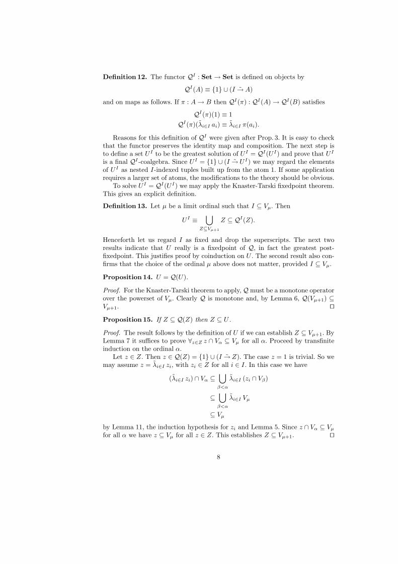
Definition 12. The functor QI : Set→ Set is defined on objects by

QI(A) ≡ {1} ∪ (I →A)

and on maps as follows. If π : A→ B then QI(π) : QI(A)→ QI(B) satisfies

QI(π)(1) ≡ 1QI(π)(λi∈I ai) ≡ λi∈I π(ai).

Reasons for this definition of QI were given after Prop. 3. It is easy to checkthat the functor preserves the identity map and composition. The next step isto define a set U I to be the greatest solution of U I = QI(U I) and prove that U I

is a final QI -coalgebra. Since U I = {1} ∪ (I → U I) we may regard the elementsof U I as nested I-indexed tuples built up from the atom 1. If some applicationrequires a larger set of atoms, the modifications to the theory should be obvious.

To solve U I = QI(U I) we may apply the Knaster-Tarski fixedpoint theorem.This gives an explicit definition.

Definition 13. Let µ be a limit ordinal such that I ⊆ Vµ. Then

U I ≡⋃

Z⊆Vµ+1

Z ⊆ QI(Z).

Henceforth let us regard I as fixed and drop the superscripts. The next tworesults indicate that U really is a fixedpoint of Q, in fact the greatest post-fixedpoint. This justifies proof by coinduction on U . The second result also con-firms that the choice of the ordinal µ above does not matter, provided I ⊆ Vµ.

Proposition 14. U = Q(U).

Proof. For the Knaster-Tarski theorem to apply,Qmust be a monotone operatorover the powerset of Vµ. Clearly Q is monotone and, by Lemma 6, Q(Vµ+1) ⊆Vµ+1. ut

Proposition 15. If Z ⊆ Q(Z) then Z ⊆ U .

Proof. The result follows by the definition of U if we can establish Z ⊆ Vµ+1. ByLemma 7 it suffices to prove ∀z∈Z z ∩ Vα ⊆ Vµ for all α. Proceed by transfiniteinduction on the ordinal α.

Let z ∈ Z. Then z ∈ Q(Z) = {1} ∪ (I → Z). The case z = 1 is trivial. So wemay assume z = λi∈I zi, with zi ∈ Z for all i ∈ I. In this case we have

(λi∈I zi) ∩ Vα ⊆⋃β<α

λi∈I (zi ∩ Vβ)

⊆⋃β<α

λi∈I Vµ

⊆ Vµby Lemma 11, the induction hypothesis for zi and Lemma 5. Since z ∩ Vα ⊆ Vµfor all α we have z ⊆ Vµ for all z ∈ Z. This establishes Z ⊆ Vµ+1. ut

8

3.2 U is a Final Coalgebra

To prove that U is a final coalgebra requires showing that for every map f : A→Q(A) there exists a unique map π : A→ U such that π = Q(π) ◦ f :

Aπ - U

‖‖‖f

?‖‖

Q(A)Q(π)- Q(U)

For the remainder of this section, let the set A and the map f : A → Q(A)be fixed.

Lemma 16. There exists π : A→ U such that π(a) = Q(π)(f(a)) for all a ∈ A.

Proof. The function π is defined by π(a) ≡⋃n<ω πn(a), where {πn}n<ω is as

follows:

π0(a) ≡ 0πn+1(a) ≡ Q(πn)(f(a))

Suppose a ∈ A and prove π(a) = Q(π)(f(a)) by cases. If f(a) = 1 then theequation reduces to 1 = 1. If f(a) = λi∈I ai then simple continuity reasoningestablishes the equation:

π(a) =⋃n<ω

πn(a)

=⋃n<ω

πn+1(a)

=⋃n<ω

λi∈I πn(ai)

= λi∈I⋃n<ω

πn(ai)

= λi∈I π(ai)= Q(π)(λi∈I ai)= Q(π)(f(a))

To show π : A → U , use coinduction (Prop. 15). Let Z = {π(a) | a ∈ A}and prove Z ⊆ Q(Z). If z ∈ Z then z = π(a) for some a ∈ A. There are twocases, as usual. If f(a) = 1 then z = 1 ∈ Q(Z) and if f(a) = λi∈I ai thenz = λi∈I π(ai) ∈ Q(Z).

Since U is the greatest post-fixedpoint of Q, this establishes Z ⊆ U . Andsince Z is the range of π, this establishes π : A→ U . ut

9

Lemma 17. If π = Q(π) ◦ f and π′ = Q(π′) ◦ f then π = π′.

Proof. Again using Lemma 7, let us use transfinite induction on the ordinal ξ toprove

∀a∈A π(a) ∩ Vξ ⊆ π′(a).

Let a ∈ A. If f(a) = 1 then π(a) = π′(a) = 1. If f(a) = λi∈I ai then

π(a) ∩ Vξ = (λi∈I π(ai)) ∩ Vξ⊆⋃η<ξ

λi∈I (π(ai) ∩ Vη)

⊆⋃η<ξ

λi∈I π′(ai)

= π′(a)

using the hypothesis, Lemma 11, the induction hypothesis for η < ξ and mono-tonicity of λ.

Since π(a) ∩ Vξ ⊆ π′(a) for every ordinal ξ, we have π(a) ⊆ π′(a). By sym-metry we have π′(a) ⊆ π(a) and therefore π(a) = π′(a) for all a ∈ A. ut

Theorem 18. U is a final Q-coalgebra.

Proof. Immediate by the previous two lemmas. ut

4 Solutions of Equations

In his development of set theory with AFA, Aczel [2] defines systems of set-equations and proves the Solution Lemma: each system has a unique solution.Aczel introduces a class X of variables and a class VX of sets built up fromvariables (but not themselves variables). His Substitution Lemma says that anyassignment f : X → V of sets to variables can be extended to a substitutionfunction f : Vx → V . Aczel uses these lemmas to exhibit a unique morphism forhis Special Final Coalgebra Theorem.

Aczel proves the Solution and Substitution Lemmas using concrete set theory,but in Rutten and Turi’s categorical presentation the proofs are much shorter. Akey fact in their development is that V is (assuming AFA) a final P-coalgebra.My presentation is similar, replacing V by U , P by Q and AFA by Theorem 18.Also I replace the category of classes by the category of sets, but this I think isonly a matter of taste.

4.1 Preliminaries: the Binary Sum Functor

Recall that + is the variant form of disjoint sum, defined by A+B ≡ ({0}×A)∪({1}×B). It is a coproduct in the category Set, which means that for every pair

10

of maps f : A→ C and g : B → C there exists a unique map [f, g] : A +B → Cmaking the diagram commute:

A˜Inl- A +B �

˜InrB

@@@f @@

@R ?

[f, g]

��� g���

C

Here the injections ˜Inl : A→ A +B and ˜Inr : B → A +B and the case analysisoperator [f, g] are defined in the obvious way.

To make + into a functor we must define its action on maps. If j : A → A′

and k : B → B′ then j + k : A +A′ → B +B′ is defined (as usual) by

j + k ≡ [ ˜Inl ◦ j, ˜Inr ◦ k]. (4)

Some obvious properties of [f, g] and of j +k are listed below for later reference.

Lemma 19. Let f : A→ C, g : B → C, h : C → D, j : A→ A′ and k : B → B′

be maps. Then

[f, g] ◦ ˜Inl = f

[f, g] ◦ ˜Inr = g

h ◦ [f, g] = [h ◦ f, h ◦ g][ ˜Inl , ˜Inr ] = idA+B

[f, g] ◦ (j + k) = [f ◦ j, g ◦ k](j + k) ◦ ˜Inl = ˜Inl ◦ j(j + k) ◦ ˜Inr = ˜Inr ◦ k

4.2 An Expanded Version of U

Let X be a set of variables or indeterminates for use in equations. The set U IX isconstructed in the same way as U I except that each level contains a copy of X.Thus an element of U IX is just like an element of U I except that it may containelements of X at each stage in its construction. In formalizing equations betweensets, each left-hand side will consist of a variable from X while each right-handside will be drawn from U IX . The definition of U IX closely resembles that of U I .

Definition 20. Let µ be a limit ordinal such that X ∪ I ⊆ Vµ. Then

U I ≡⋃

Z⊆Vµ+1

Z ⊆ QI(X + Z).

Let us again drop the superscript I. The proof of the following result isomitted because of its similarity to the proof for U .

11

Proposition 21. Let UX be defined as above. Then

(a) UX = Q(X + UX).(b) If Z ⊆ Q(X + Z) then Z ⊆ UX .(c) UX is the final coalgebra for the functor Q(X +−).

Proof. See Appendix A.

4.3 An Embedding

There is an obvious embedding σX : U → UX that copies an element of Uinto UX and never introduces an element of X:

σX(1) = 1σX(λi∈I ui) = λi∈I ˜Inr(σX(ui))

The equations can be summarised neatly by σX = Q( ˜Inr ◦σX). The embeddingwill be useful for creating equations with constant right-hand sides.

Although the embedding is obvious, its existence deserves to be proved. Aczelderives the analogous embedding from V into VX by direct recourse to AFA [2].Rutten and Turi [12] omit this step, which in their categorical style might bedone by showing that VX is a final coalgebra for the functor P(X +−).

Lemma 22. There exists a unique map σX : U → UX such that

σX = Q( ˜Inr ◦ σX).

Proof. Recalling the equation UX = Q(X +UX), consider the following diagram:

UσX - UX

‖‖‖Q( ˜Inr)

?‖‖

Q(X + U)Q(idX + σX)

- Q(X + UX)

Since (U,Q( ˜Inr)) is a coalgebra for Q(X +−) and UX is a final coalgebra, thereexists a unique map σX such that the diagram commutes. Now

σX = Q(idX + σX) ◦ Q( ˜Inr)= Q((idX + σX) ◦ ˜Inr)= Q( ˜Inr ◦ σX)

by Lemma 19. ut

12

4.4 Substitution

Let f : X → U be a function. Then the substitution function f : UX → Uessentially copies its argument, replacing everything of the form ˜Inl(x) by f(x)for x ∈ X. This case analysis can be expressed with the help of the [f, f ] notation:

f(1) = 1

f(λi∈I zi) = λi∈I [f, f ](zi)

These two equations can be expressed succinctly by f = Q([f, f ]).Clearly, substitution over a ‘term’ containing no ‘variables’ can have no effect.

The formal statement of this fact justifies calling σX an embedding.

Lemma 23 (Embedding). Let f : X → U and g : UX → U be functions. Ifg = Q([f, g]) then g ◦ σX = idU .

Proof. By Lemma 22 and Lemma 19 we have

g ◦ σX = Q([f, g]) ◦ Q( ˜Inr ◦ σX)= Q([f, g] ◦ ˜Inr ◦ σX)= Q(g ◦ σX).

Since U = Q(U), the following diagram commutes:

Ug ◦ σX - U

‖‖‖

‖‖‖

‖‖

‖‖

Q(U)Q(g ◦ σX)

- Q(U)

Since U is the final Q-coalgebra, it has only one homomorphism into itself,namely the identity. This yields g ◦ σX = idU . ut

4.5 Solution and Substitution Lemmas

IfX is a set of variables then a function ν : X → UX defines a system of equationsof the form x = νx for all x ∈ X. Such a system has a unique solution f : X → Usuch that f(x) = f(νx) for x ∈ X. More concisely, a solution satisfies f = f ◦ ν.

Lemma 24 (Solution). Let ν : X → UX be a function. There exist uniquefunctions f : X → U and f : UX → U such that

f = f ◦ ν and f = Q([f, f ]).

13

Proof. Recalling the equation UX = Q(X +U), consider the following diagram:

Xν - UX

π - U‖‖‖Q([ν, idUX ])

?‖‖

Q(UX)Q(π)- Q(U)

Since (UX ,Q([ν, idUX ])) is a Q-coalgebra and U is a final Q-coalgebra, thereexists a unique map π such that the diagram commutes. By Lemma 19 we have

π = Q(π) ◦ Q([ν, idUX ])= Q(π ◦ [ν, idUX ])= Q([π ◦ ν, π ◦ idUX ])= Q([π ◦ ν, π])

Putting f = π and f = π ◦ ν yields the desired functions. As for uniqueness, iff = f ◦ ν and f = Q([f, f ]) then f = π by finality of U . ut

In this proof, note that Q([ν, idUX ]) substitutes using ν but only to depthone. The following lemma justifies the f notation for substitution by f . Theidea is to convert f : X → U into a trivial system of equations, then solve them.

Lemma 25 (Substitution). Let f : X → U be a function. There exists aunique function f : UX → U such that f = Q([f, f ]).

Proof. Consider the composed map σX ◦ f : X → UX . Apply the SolutionLemma with ν = σX ◦ f , obtaining maps g : X → U and g : UX → U such thatg = g ◦ ν and g = Q([g, g]). Now

g = g ◦ σX ◦ f = f

by Lemma 23. Putting f = g we obtain f = Q([f, f ]). Uniqueness follows by theuniqueness property of the Solution Lemma. ut

I should prefer to prove the Substitution Lemma earlier, but the simplestproof seems to rely on the Solution Lemma. Turi has pointed out (by electronicmail) that the Substitution Lemma has a trivial proof if UX is defined to bean initial algebra rather than a final coalgebra. But then UX would containonly finite constructions; the embedding σX : U → UX would not exist; non-well-founded objects obtained via the Solution Lemma could not participate infurther set equations.

14

4.6 Special Final Coalgebra Theorem

The main theorem applies to functors that are uniform on maps. This notion isdue to Aczel [2], but I follow Rutten and Turi’s [12] formulation.

We shall no longer work in the category Set of sets but rather in the fullsubcategory SetU whose objects are the subsets of U . Recall that U , in turn,depends upon the choice of index set I; we can make U as large as necessary.

Definition 26. A functor F : SetU → SetU is uniform on maps if for all A ⊆ Uthere exists a mapping φA : F (A)→ UA such that

F (h) = h ◦ φA for all h : A→ U.

The mapping φA is called the UA translation.

Let us only consider functors that preserve inclusion maps. This is a naturalrestriction since all functors preserve identity maps, and inclusion maps areidentity maps when regarded as sets. All such functors on SetU have fixedpoints.

Lemma 27. If the functor F : SetU → SetU preserves inclusions then thereexists an object JF : SetU such that JF is the greatest fixedpoint and greatestpost-fixedpoint of F .

Proof. Apply the Knaster-Tarski fixedpoint theorem to the lattice of subsetsof U . The functor F is necessarily monotone because it preserves inclusions; ifι : A→ B then F (ι) : F (A)→ F (B); thus if A ⊆ B then F (A) ⊆ F (B). ut

Theorem 28 (Special Final Coalgebra). If the functor F : SetU → SetUpreserves inclusions and is uniform on maps then JF is a final F -coalgebra.

Proof. Let (A, f) be an F -coalgebra. We must exhibit a unique map h : A→ JFsuch that h = F (h) ◦ f :

Ah - JF

‖‖‖f

?‖‖

F (A)F (h)- F (JF )

Since F is uniform on maps, h = F (h) ◦ f is equivalent to h = h ◦ φA ◦ f .Such a map h is precisely a solution of the system of equations a = φA(f(a)) fora ∈ A. Applying the Solution Lemma with ν = φA ◦ f , we obtain a unique maph : A→ U such that h = F (h) ◦ f .

15

A standard coinduction argument proves h : A → JF . Writing h“A for theimage of A under h, we have

h“A = (F (h) ◦ f)“A= F (h)“(f“A)⊆ F (h)“F (A)⊆ F (h“A)

since h : A→ h“A and F (h) : F (A)→ F (h“A).The range of h is thus a post-fixedpoint of F and is contained in the greatest

post-fixedpoint, namely JF . ut

5 Functors Uniform on Maps

If F is uniform on maps then, in essence, its effect upon a map h : A→ U can beexpressed as the substitution of h over a pattern derived from the argument; ifb ∈ F (A) then F (h)(b) = h(φA(b)). Most natural functors are uniform on mapsbut there is at least one glaring exception. Let us examine some typical cases,starting with a very easy one.

5.1 The Constant Functor

If C ⊆ U then let KC be the constant functor such that KC(A) = C for allA : SetU and such that KC(f) = idC for all maps f : A→ A′.

Proposition 29. If C : SetU then the constant functor KC : SetU → SetU isuniform on maps.

Proof. Let A be a set such that A : SetU . Define φA : C → UA by φA(c) = σA(c)for all c ∈ C. Now

KC(h)(c) = c = (h ◦ σA)(c) = (h ◦ φA)(c)

for all c ∈ C by Lemma 23. ut

5.2 Binary Product

The set U satisfies the inclusion U × U ⊆ U . So it is easy to see that × :SetU × SetU → SetU is a functor when extended to maps in the standard way.If f : A → A′ and g : B → B′ are maps then f × g : A × B → A′ × B′ is themap that takes 〈a; b〉 to 〈f(a); g(b)〉.

Proposition 30. If F , G : SetU → SetU are uniform on maps, then the functor

F (−) ×G(−) : SetU → SetU

is uniform on maps.

16

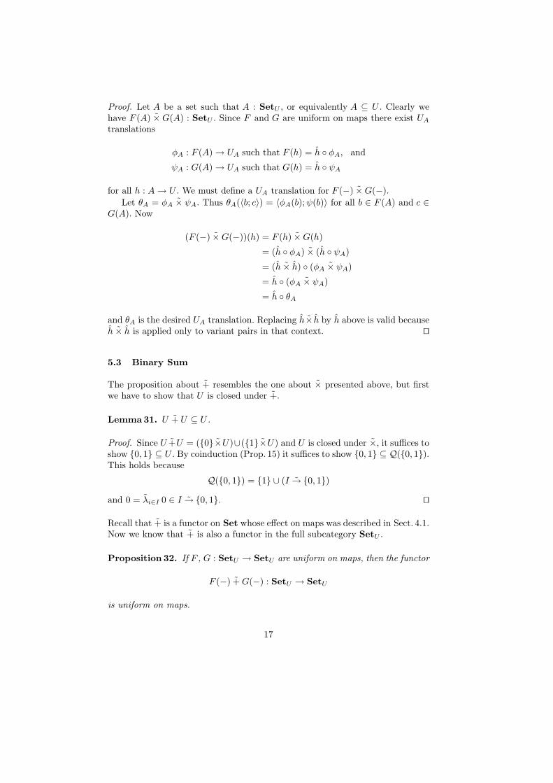
Proof. Let A be a set such that A : SetU , or equivalently A ⊆ U . Clearly wehave F (A) × G(A) : SetU . Since F and G are uniform on maps there exist UAtranslations

φA : F (A)→ UA such that F (h) = h ◦ φA, and

ψA : G(A)→ UA such that G(h) = h ◦ ψA

for all h : A→ U . We must define a UA translation for F (−) ×G(−).Let θA = φA × ψA. Thus θA(〈b; c〉) = 〈φA(b);ψ(b)〉 for all b ∈ F (A) and c ∈

G(A). Now

(F (−) ×G(−))(h) = F (h) ×G(h)

= (h ◦ φA) × (h ◦ ψA)

= (h × h) ◦ (φA × ψA)

= h ◦ (φA × ψA)

= h ◦ θA

and θA is the desired UA translation. Replacing h× h by h above is valid becauseh × h is applied only to variant pairs in that context. ut

5.3 Binary Sum

The proposition about + resembles the one about × presented above, but firstwe have to show that U is closed under +.

Lemma 31. U + U ⊆ U .

Proof. Since U +U = ({0}×U)∪({1}×U) and U is closed under ×, it suffices toshow {0, 1} ⊆ U . By coinduction (Prop. 15) it suffices to show {0, 1} ⊆ Q({0, 1}).This holds because

Q({0, 1}) = {1} ∪ (I → {0, 1})

and 0 = λi∈I 0 ∈ I → {0, 1}. ut

Recall that + is a functor on Set whose effect on maps was described in Sect. 4.1.Now we know that + is also a functor in the full subcategory SetU .

Proposition 32. If F , G : SetU → SetU are uniform on maps, then the functor

F (−) +G(−) : SetU → SetU

is uniform on maps.

17

Proof. Let A be a set such that A : SetU . Then F (A) +G(A) : SetU and thereexist UA translations

φA : F (A)→ UA such that F (h) = h ◦ φA, and

ψA : G(A)→ UA such that G(h) = h ◦ ψAfor all h : A→ U .

Let θA = φA + ψA. Then

(F (−) +G(−))(h) = F (h) +G(h)

= (h ◦ φA) + (h ◦ ψA)

= (h + h) ◦ (φA + ψA)

= h ◦ (φA + ψA)

= h ◦ θAand θA is the desired UA translation. ut

5.4 Sum of a Family of Sets

Let {Bx}x∈C be a C-indexed family of sets. If C ⊆ U and Bx ⊆ U for all x ∈ Cthen we have

∑x∈C

Bx ⊆ U . Note that∑x∈C

Bx is the usual generalisation of C ×Bto allow B to depend upon x ∈ C; the two functors have the same effect uponmaps. But the proposition about

∑differs in one key respect from that about ×:

the index set is not given by a functor but is constant.

Proposition 33. If C : SetU and {Fx : SetU → SetU}x∈C is a C-indexedfamily of functors that are uniform on maps, then the functor∑

x∈CFx(−) : SetU → SetU

is uniform on maps.

Proof. Let A be a set such that A : SetU . Then∑x∈C

Fx(A) : SetU . There exists

a UA translation φx,A : Fx(A) → UA such that Fx(h) = h ◦ φx,A for all x ∈ Aand h : A→ U .

The UA translation for∑x∈C

Fx(−), called θA, is defined by

θA(〈x; y〉) = 〈σA(x), φx,A(y)〉for all x ∈ C and c ∈ Fx(A). Recall that σA is the inclusion map from U into UA.Now by Lemma 23 we have

h(θA(〈x; y〉)) = h(〈σA(x), φx,A(y)〉)= 〈h(σA(x)), h(φx,A(y))〉= 〈x, Fx(h)〉

= (∑x∈C

Fx(h))(〈x; y〉)

18

which proves h ◦ θA = (∑x∈C

Fx(−))(h). ut

5.5 Product of a Family of Sets

Again let {Bx}x∈C be a C-indexed family of sets. If C ⊆ I (not C ⊆ U as above!)and Bx ⊆ U for all x ∈ C then

∏x∈C

Bx ⊆ I → U ⊆ U .

Thus∏

: SetIU → SetU is a functor whose effect on maps is as follows. If{fx : Bx → B′x}x∈C is a C-indexed family of maps then

∏x∈C

fx :∏x∈C

Bx →∏x∈C

B′x

is the usual pointwise map that takes λx∈Cbx to λx∈Cfx(bx).

Proposition 34. If C ⊆ I and {Fx : SetU → SetU}x∈C is a C-indexed familyof functors that are uniform on maps, then the functor

∏x∈C

Fx(−) : SetU → SetU

is uniform on maps.

Proof. Let A be a set such that A : SetU . Then∏x∈C

Fx(A) : SetU . There exists

a UA translation φx,A : Fx(A) → UA such that Fx(h) = h ◦ φx,A for all x ∈ Aand h : A→ U .

Let θA =∏x∈C

φx,A. Now

(∏x∈C

Fx(−))(h) =∏x∈C

Fx(h)

=∏x∈C

h ◦ φx,A

= (∏x∈C

h) ◦ (∏x∈C

φx,A)

= h ◦ (∏x∈C

φx,A)

= h ◦ θA

and θA is the desired UA translation. ut

19

5.6 The Identity Functor

These results suggest that any functor that operates on ‘constructions’ in a point-wise fashion is probably uniform on maps. But there is one glaring exception.

Proposition 35. The identity functor Id : SetU → SetU is not uniform onmaps.

Proof. Suppose Id : SetU → SetU is uniform on maps. Then if A ⊆ U thenthere is a mapping φA : A→ UA such that h = h ◦ φA for all h : A→ U .

Let A = {1} and define h1, h2 : {1} → U by h1(1) = 1 and h2(1) = 〈1; 1〉.Then 1 = h1(φA(1)); by the definition of substitution, this implies φA(1) = 1.Also 〈1; 1〉 = h2(φA(1)); by the definition of substitution, this implies φA(1) =〈a; b〉 for some a, b ∈ A + UA. But then 1 = 〈a; b〉, which is absurd. ut

An alternative proof uses the Special Final Coalgebra Theorem. If Id is uni-form on maps then JId is a final Id-coalgebra. But a final Id-coalgebra must bea singleton set, while JId = U and U contains 0 and 1 as elements.

This circumstance is awkward. The natural way of constructing suitable func-tors is to combine constant and identity functors by products, sums, etc. Sincethe identity functor is not uniform on maps, this approach fails. Various simi-lar functors are uniform on maps, such as − × K{0} and − × −; both have thesingleton set {0} as their greatest fixedpoint. Assuming AFA does not help; theidentity functor is not uniform on maps in Aczel’s system either.

6 Conclusions

In semantics it is not customary to worry about the construction of a particularobject provided it has the desired abstract properties. From this point of view,the general theorems of Aczel and Mendler [3] and Barr [4] yield final coalgebrasfor a great many functors.

But there is an undoubted interest in Aczel’s weaker final coalgebra theorem,proved using the Anti-Foundation Axiom (AFA) [2]. Its appeal is its concrete-ness. The set of streams over A is simply the greatest fixedpoint of the func-tor A × −, which is also that functor’s final coalgebra. Its elements are easilyvisualised objects of the form 〈a0, a1, a2, . . .〉.

The original motivation for my work was to treat streams and other infi-nite data structures. I wished to use the standard ZF axiom system as it wasautomated using Isabelle. Thomas Forster suggested that Quine’s treatment ofordered pairs might help. Generalizing this treatment led to the new defini-tion of functions (and thus infinite streams), in order to compare the approachwith AFA. This part of the work closely follows Aczel, and Rutten and Turi [12],from the Substitution Lemma onwards.

My Special Final Coalgebra Theorem is less general than Aczel’s, especiallyas regards concurrency. Here is a typical example. Let Pf be the finite powersetoperator, which returns the set of all finite subsets of its argument. Consider the

20

set P of processes defined as the final coalgebra of Pf (A × −). With AFA thefinal coalgebra is the greatest solution of P = Pf (A× P ), and if p ∈ P then

p = {〈a1, p1〉, . . . , 〈an, pn〉}

with n < ω, a1, . . . , an ∈ A and p1, . . . , pn ∈ P . My approach does not handlegeneral set constructions, only variant tuples and functions; I do not know howto model Pf respecting set equalities such as {x, y} = {y, x} = {x, y, x}.

My approach works best in its original application, infinite data structures.We can model the main constructions in Uω. Since Uω ⊆ Vω+1, each infinite datastructure is a subset of Vω and thus is a set of hereditarily finite sets.3 Section 2.1discussed infinite streams. The set S of streams over A is the greatest solutionof S = A × S, and is the final coalgebra of the functor A × −.

Thus we have an account of non-well-founded phenomena that is concreteenough to be understood directly. One can argue about the constructive validityof the cumulative hierarchy, but Vω is uncontroversial even from an intuitionisticviewpoint. In contrast the general final coalgebra theorems [3, 4], with theirquotient-of-sum constructions, are anything but concrete.

Aczel has shown that by adopting AFA we can obtain final coalgebras asgreatest fixedpoints, dualising a standard result about initial algebras. My ap-proach is another way of doing the same thing, though for fewer functors.Whether or not one choose to adopt AFA hinges on a number of issues: philosoph-ical, theoretical, practical. Variant tuples and functions are a simple alternative.

References

1. Abramsky, S., The lazy lambda calculus, In Resesarch Topics in Functional Pro-gramming, D. A. Turner, Ed. Addison-Wesley, 1977, pp. 65–116

2. Aczel, P., Non-Well-Founded Sets, CSLI, 19883. Aczel, P., Mendler, N., A final coalgebra theorem, In Category Theory and

Computer Science (1989), D. H. Pitt, D. E. Rydeheard, P. Dybjer, A. M. Pitts,,A. Poigne, Eds., Springer, pp. 356–365, LNCS 389

4. Barr, M., Terminal coalgebras in well-founded set theory, Theoretical Comput.Sci. 114, 2 (1993), 299–315

5. Kunen, K., Set Theory: An Introduction to Independence Proofs, North-Holland,1980

6. Milner, R., Communication and Concurrency, Prentice-Hall, 19897. Milner, R., Tofte, M., Co-induction in relational semantics, Theoretical Comput.

Sci. 87 (1991), 209–2208. Paulson, L. C., Set theory for verification: I. From foundations to functions, J.

Auto. Reas. 11, 3 (1993), 353–3899. Paulson, L. C., Set theory for verification: II. Induction and recursion, Tech. Rep.

312, Comp. Lab., Univ. Cambridge, 1993, To appear in J. Auto. Reas.10. Paulson, L. C., A fixedpoint approach to implementing (co)inductive definitions,

In 12th Conf. Auto. Deduct. (1994), A. Bundy, Ed., Springer, pp. 148–161, LNAI814

3 An hereditarily finite set is one built in finitely many stages from the empty set.

21

11. Quine, W. V., On ordered pairs and relations, In Selected Logic Papers. RandomHouse, 1966, ch. VIII, pp. 110–113, Orginally published 1945–6

12. Rutten, J. J. M. M., Turi, D., On the foundations of final semantics: Non-standardsets, metric spaces, partial orders, In Semantics: Foundations and Applications(1993), J. de Bakker, W.-P. de Roever,, G. Rozenberg, Eds., Springer, pp. 477–530, LNCS 666

22

A Proof of Prop. 21

Abbreviate the functor Q(X + −) as QX . This simplifies the statement of theProposition:

Proposition. Let UX =⋃Z⊆Vµ+1

Z ⊆ QX(Z). Then

(a) UX = QX(UX).(b) If Z ⊆ QX(Z) then Z ⊆ UX .(c) UX is the final QX-coalgebra.

Proof of (a). Apply the Knaster-Tarski theorem. Clearly QX is monotone; byLemma 6, QX(Vµ+1) ⊆ Vµ+1. ut

Before continuing, we need some more elementary facts about the cumulativehierarchy.

Lemma 36. If α is an ordinal then

A×B ⊆ Vα implies A,B ⊆ VαA+B ⊆ Vα implies A,B ⊆ Vα

A ×B ⊆ Vα+1 implies A,B ⊆ Vα+1

A +B ⊆ Vα+1 implies A,B ⊆ Vα+1

Proof. The first part holds by Lemma 10 and the transitivity of Vα. The otherparts hold by similar tedious reasoning from the definitions. ut

We now tackle the next part of Prop. 21.

Proof of (b). Use the definition of UX after first establishing Z ⊆ Vµ+1. By theprevious Lemma, it suffices to prove X + Z ⊆ Vµ+1. By Lemma 7, it suffices toprove

∀w∈X+Z w ∩ Vα ⊆ Vµfor all α. Proceed by transfinite induction on the ordinal α.

Let w ∈ X + Z. There are two cases. The first case is w = 〈0;x〉 = 0 + x forx ∈ X. Since X ⊆ Vµ, clearly 0 + x ⊆ Vµ. The second case is w = 〈1; z〉 = 1 + zfor z ∈ Z. We must show 1 + z ⊆ Vµ; by Lemma 4 it suffices to show z ⊆ Vµ.

Since z ∈ Z, we have z ∈ QX(Z) = {1} ∪ (I → X + Z). The case z = 1 istrivial. So we may assume z = λi∈I wi, with wi ∈ X + Z for all i ∈ I. In thiscase we have

(λi∈I wi) ∩ Vα ⊆⋃β<α

λi∈I (wi ∩ Vβ)

⊆⋃β<α

λi∈I Vµ

⊆ Vµby Lemma 11, the induction hypothesis for wi and Lemma 5. Since w∩Vα ⊆ Vµfor all α we have w ⊆ Vµ for all w ∈ X + Z. This establishes X + Z ⊆ Vµ+1 asrequired. ut

23

The final part of Prop. 21 is that UX is the final QX -coalgebra. This requiresshowing that for every map f : A→ QX(A) there exists a unique map π : A→UX such that π = QX(π) ◦ f :

Aπ - UX

‖‖‖f

?‖‖

QX(A)QX(π)

- QX(UX)

Let the set A and the map f : A→ QX(A) be fixed, and consider each propertyseparately. Note that the functor QX operates on maps as follows:

QX(π)(λi∈I ai) = λi∈I (idX + π)(ai)

Lemma 37. There exists π : A → UX such that π(a) = QX(π)(f(a)) for alla ∈ A.

Proof. The function π is defined by π(a) ≡⋃n<ω πn(a), where {πn}n<ω is as

follows:

π0(a) ≡ 0πn+1(a) ≡ QX(πn)(f(a))

Suppose a ∈ A and prove π(a) = Q(π)(f(a)) by cases. If f(a) = 1 thenthe equation reduces to 1 = 1. The other possibility is f(a) = λi∈I bi wherebi ∈ X +A if i ∈ I. Continuity reasoning, using the previous lemma, establishesthe equation:

π(a) =⋃n<ω

πn(a)

=⋃n<ω

πn+1(a)

=⋃n<ω

QX(πn)(λi∈I bi)

=⋃n<ω

λi∈I (idX + πn)(bi)

= λi∈I⋃n<ω

(idX + πn)(bi)

= λi∈I (idX + π)(bi)= QX(π)(λi∈I bi)= QX(π)(f(a))

24

Note that⋃n<ω(idX + πn)(bi) = (idX + π)(bi) above holds by case analysis on

bi ∈ X +A and continuity of the variant injections.To show π : A → UX , use coinduction. Let Z = {π(a) | a ∈ A} and prove

Z ⊆ QX(Z). If z ∈ Z then z = π(a) for some a ∈ A. There are two cases, asusual. If f(a) = 1 then z = 1 ∈ QX(Z). If f(a) = λi∈I bi (where bi ∈ X + A)then

z = π(a) = QX(π)(λi∈I bi) = λi∈I (idX + π)(bi) ∈ Q(X + Z) = QX(Z).

Since UX is the greatest post-fixedpoint of QX , this establishes Z ⊆ UX . Andsince Z is the range of π, this establishes π : A→ UX . ut

Lemma 38. If π = QX(π) ◦ f and π′ = QX(π′) ◦ f then π = π′.

Proof. Using Lemma 7, let us use transfinite induction on the ordinal ξ to prove

∀a∈A π(a) ∩ Vξ ⊆ π′(a).

Let a ∈ A. If f(a) = 1 then π(a) = π′(a) = 1. If f(a) = λi∈I bi (where bi ∈ X+A)then

π(a) ∩ Vξ = (λi∈I (idX + π)(bi)) ∩ Vξ⊆⋃η<ξ

λi∈I ((idX + π)(bi) ∩ Vη)

⊆ λi∈I (idX + π′)(bi)= π′(a)

using the hypothesis, Lemma 11 and monotonicity of λ. The reasoning also uses

(idX + π)(bi) ∩ Vη ⊆ (idX + π′)(bi),

which holds by case analysis on bi ∈ X +A, a further application of Lemma 11,and the induction hypothesis for η′ where η′ < η < ξ.

Since π(a) ∩ Vξ ⊆ π′(a) for every ordinal ξ, we have π(a) ⊆ π′(a). By sym-metry we have π′(a) ⊆ π(a) and therefore π(a) = π′(a) for all a ∈ A. ut

Theorem 39. UX is a final QX-coalgebra.

Proof. Immediate by the previous two lemmas. ut

This article was processed using the LaTEX macro package with LLNCS style

25